Joint Probabilities within Random Permutations

Abstract

A celebrated analogy between prime factorizations of integers and cycle decompositions of permutations is explored here.  Asymptotic formulas characterizing semismooth numbers (possessing at most several large factors) carry over to random permutations.  We offer a survey of practical methods for computing relevant probabilities of a bivariate or trivariate flavor.

Let $\Lambda_{r}$ denote the length of the $r^{\text{th}}$ longest cycle in an $n$-permutation, chosen uniformly at random.  If the permutation has no $r^{\text{th}}$ cycle, then its $r^{\text{th}}$ longest cycle is defined to have length $0$.  The case $r=1$ has attracted widespread attention [1, 2].  We have

$$\begin{array}[c]{ccc}\lim\limits_{n\rightarrow\infty}\mathbb{P}\left\{\Lambda_{1}\leq x\,n\right\}=\rho\left(\dfrac{1}{x}\right),&&0<x\leq 1\end{array}$$

where $\rho=\rho_{1}$ is Dickman’s function:

$$\begin{array}[c]{ccc}\xi\,\rho_{1}^{\prime}(\xi)+\rho_{1}(\xi-1)=0\text{ for }\xi>1,&&\rho_{1}(\xi)=1\text{ for }0\leq\xi\leq 1.\end{array}$$

Also $\rho_{1}(\xi)=0$ for $\xi<0$.  More generally [3, 4],

$$\begin{array}[c]{ccc}\lim\limits_{n\rightarrow\infty}\mathbb{P}\left\{\Lambda_{2}\leq y\,n\right\}=\rho_{2}\left(\dfrac{1}{y}\right),&&0<y\leq\dfrac{1}{2};\end{array}$$

$$\begin{array}[c]{ccc}\lim\limits_{n\rightarrow\infty}\mathbb{P}\left\{\Lambda_{3}\leq z\,n\right\}=\rho_{3}\left(\dfrac{1}{z}\right),&&0<z\leq\dfrac{1}{3};\end{array}$$

$$\begin{array}[c]{ccc}\lim\limits_{n\rightarrow\infty}\mathbb{P}\left\{\Lambda_{4}\leq w\,n\right\}=\rho_{4}\left(\dfrac{1}{w}\right),&&0<w\leq\dfrac{1}{4}\end{array}$$

where

$$\begin{array}[c]{ccc}\xi\,\rho_{r}^{\prime}(\xi)+\rho_{r}(\xi-1)=\rho_{r-1}(\xi-1)\text{ for }\xi>1,&&\rho_{r}(\xi)=1\text{ for }0\leq\xi\leq 1\end{array}$$

for $r=2,3,4$.  It is known that, as $n\rightarrow\infty$, the infinite sequence $\frac{1}{n}\left(\Lambda_{1},\Lambda_{2},\Lambda_{3},\Lambda_{4},\ldots\right)$ converges to what is called the Poisson-Dirichlet distribution with parameter $1$.  Our interest is in the practicalities of computing this distribution, not for infinite sequences, but merely the finite section $\frac{1}{n}\left(\Lambda_{1},\Lambda_{2},\Lambda_{3},\Lambda_{4}\right)$.  A special case of Billingsley’s formula for the corresponding density is [5, 6, 7, 8, 9]:

$$f_{1234}(x,y,z,w)=\dfrac{1}{x\,y\,z\,w}\,\rho\left(\dfrac{1-x-y-z-w}{w}\right),$$

$$\begin{array}[c]{ccc}1>x>y>z>w>0,&&x+y+z+w<1.\end{array}$$

More special cases include

$$\begin{array}[c]{ccccc}f_{123}(x,y,z)=\dfrac{1}{x\,y\,z}\,\rho\left(\dfrac{1-x-y-z}{z}\right),&&1>x>y>z>0,&&x+y+z<1;\end{array}$$

$$\begin{array}[c]{ccccc}f_{12}(x,y)=\dfrac{1}{x\,y}\,\rho\left(\dfrac{1-x-y}{y}\right),&&1>x>y>0,&&x+y<1;\end{array}$$

$$\begin{array}[c]{ccc}f_{1}(x)=\dfrac{1}{x}\,\rho\left(\dfrac{1-x}{x}\right)=\dfrac{d}{dx}\rho_{1}\left(\dfrac{1}{x}\right),&&1>x>0;\end{array}$$

$$\begin{array}[c]{ccc}f_{2}(y)=\dfrac{d}{dy}\rho_{2}\left(\dfrac{1}{y}\right),&&\dfrac{1}{2}>y>0\end{array}$$

and likewise for $f_{3}(z)$, $f_{4}(w)$, but no compact representations for $f_{13}(x,z)$, $f_{14}(x,w)$, $f_{23}(y,z)$ seem to be available.

For example,

$$\lim\limits_{n\rightarrow\infty}\mathbb{P}\left\{\frac{\Lambda_{1}}{n}\leq\frac{1}{2}\text{ \& }\frac{\Lambda_{2}}{n}\leq\frac{1}{3}\right\} =\lim\limits_{n\rightarrow\infty}\mathbb{P}\left\{\frac{\Lambda_{1}}{n}\leq\frac{1}{2}\right\}-\lim\limits_{n\rightarrow\infty}\mathbb{P}\left\{\frac{\Lambda_{1}}{n}\leq\frac{1}{2}\text{ \& }\frac{1}{3}<\frac{\Lambda_{2}}{n}\leq\frac{1}{2}\right\}$$

$$={\displaystyle\int\limits_{0}^{1/2}}f_{1}(x)dx-{\displaystyle\int\limits_{1/3}^{1/2}}\,{\displaystyle\int\limits_{1/3}^{x}}f_{12}(x,y)dy\,dx=\rho_{1}(2)-{\displaystyle\int\limits_{1/3}^{1/2}}\,{\displaystyle\int\limits_{1/3}^{x}}\frac{dy\,dx}{x\,y}$$

$$=\left(1-\ln(2)\right)-\frac{1}{2}\ln\left(\frac{3}{2}\right)^{2}=0.224651842493....$$

Call this probability $A$.  It is associated with the blue$\,\cup\,$magenta$\,\cup\,$green trapezoid in Figure 1, i.e., the large isosceles triangle to the left of $y=\frac{1}{2}$ with the small orange triangle removed.  The probability $B$ associated with the orange$\,\cup\,$brown triangle is clearly

$$\lim\limits_{n\rightarrow\infty}\mathbb{P}\left\{\frac{\Lambda_{2}}{n}>\frac{1}{3}\right\} =1-\rho_{2}\left(3\right)=-\frac{\pi^{2}}{12}+\frac{\ln(3)^{2}}{2}+\operatorname*{Li}\nolimits_{2}\left(\frac{1}{3}\right)$$

$$=0.147220676959....$$

Hence

$$\lim\limits_{n\rightarrow\infty}\mathbb{P}\left\{\frac{\Lambda_{1}}{n}>\frac{1}{2}\text{ \& }\frac{\Lambda_{2}}{n}\leq\frac{1}{3}\right\}=1-A-B=0.628127480547...$$

which is associated with the yellow$\,\cup\,$red$\,\cup\,$cyan trapezoid, i.e., the large isosceles triangle to the right of $y=\frac{1}{2}$ with the small brown triangle removed.  Such tractable symbolics (for this specific case) tend to obscure difficult numerics (in general) when integrating, due to an explosive singularity of $f_{12}$ at $(x,y)=(1,0)$.  We shall devote the rest of this paper to simple methods for computing probabilities quickly and accurately.

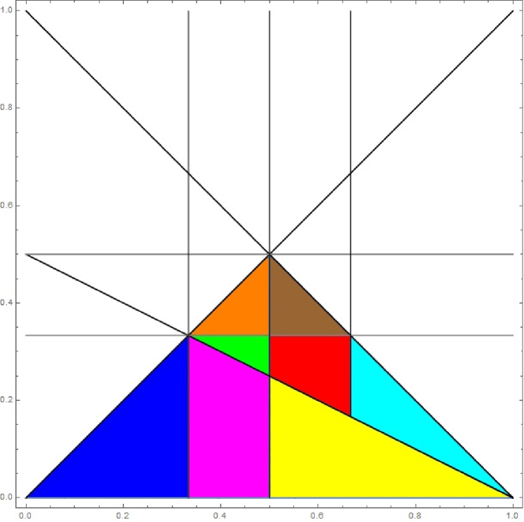
Figure 1: Domain of integration for $(\Lambda_{1},\Lambda_{2})$ example.

1 Density

Difficulties presented by the numerical integration of $f_{12}(x,y)$ are evident in Figure 2.  The surface appears to touch the $xy$-plane only when $y=0$; its prominent ridge occurs along the line $y=(1-x)/2$ because $(1-x-y)/y=1$ corresponds to a unique point of nondifferentiability for $\xi\mapsto\rho(\xi)$; its remaining boundary hovers over the broken line $y=\min\{x,1-x\}$, everywhere finite except in the vicinity of $x=0$.

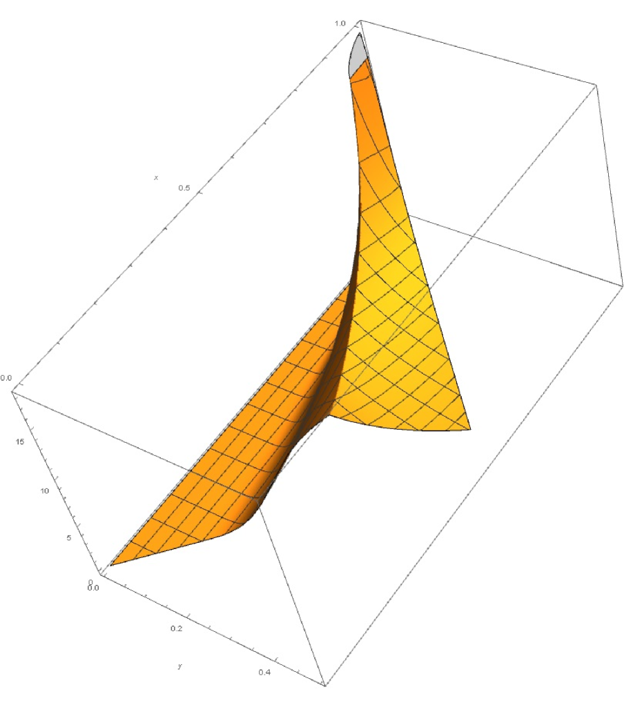
Figure 2: Probability density of $(\Lambda_{1},\Lambda_{2})$, over $0\leq y\leq 1/2$ and $y\leq x\leq 1-y.$

Complications are compounded for the three other densities (which are, in themselves, approximations).  Figure 3 contains a plot of

$$f_{13}(x,z)={\displaystyle\int\limits_{z}^{x}}f_{123}(x,y,z)dy.$$

The surface appears to touch the $xz$-plane when $z=0$ and $0<x<1/2$ simultaneously, as well as everywhere along the broken line $z=\min\{x,(1-x)/2\}$.

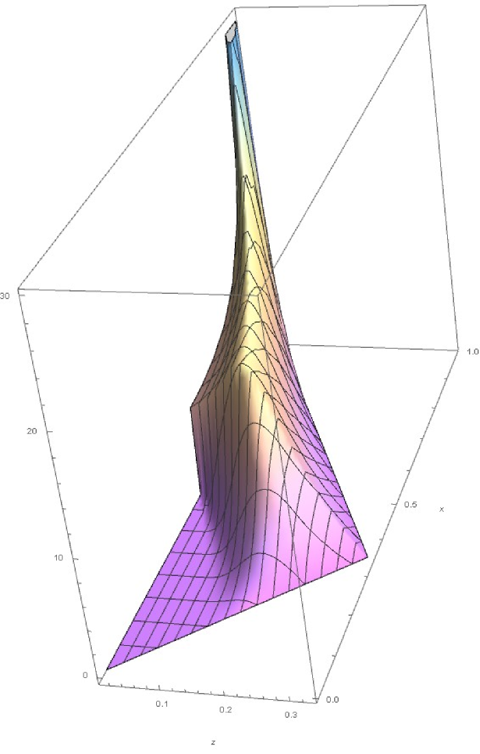
Figure 3: Probability density of $(\Lambda_{1},\Lambda_{3})$, over $0\leq z\leq 1/3$ and $z\leq x\leq 1-2z.$

Figure 4 contains a plot of

$$f_{14}(x,w)={\displaystyle\int\limits_{w}^{\min\{x,1/3\}}}\,{\displaystyle\int\limits_{z}^{x}}f_{1234}(x,y,z,w)dy\,dz.$$

The (precipitously rising) surface appears to touch the $xw$-plane only when $w=0$ and $0<x<1/2$ simultaneously; its remaining boundary hovers over the broken line $w=\min\{x,(1-x)/3\}$, everywhere finite except in the vicinity of $x=0$. The vertical scale is more expansive here than for the other plots.

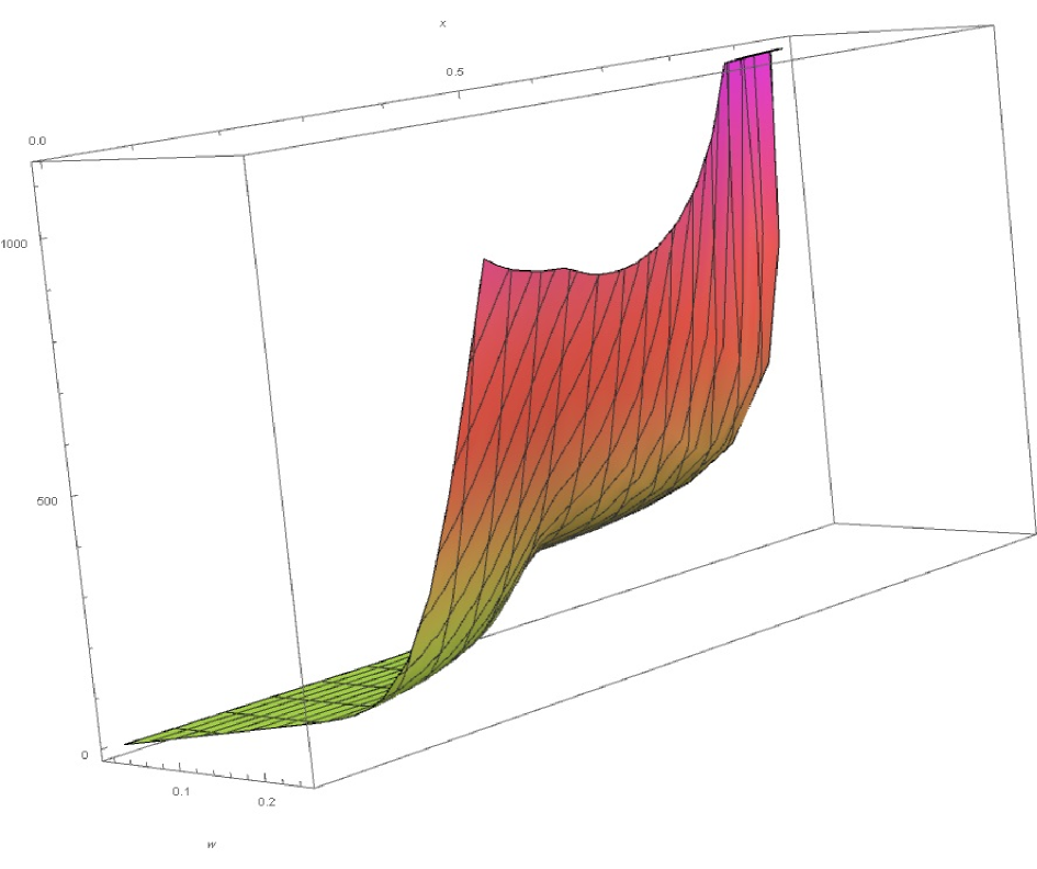
Figure 4: Probability density of $(\Lambda_{1},\Lambda_{4})$, over $0\leq w\leq 1/4$ and $w\leq x\leq 1-3w.$

Figure 5 contains a plot of

$$f_{23}(y,z)={\displaystyle\int\limits_{y}^{1}}f_{123}(x,y,z)dx.$$

The (fairly undulating) surface appears to touch the $yz$-plane only when $z=1-2y$.  Unlike the other densities, a singularity here occurs at $(y,z)=(0,0)$.

Figure 5: Probability density of $(\Lambda_{2},\Lambda_{3})$, over $0\leq z\leq 1/3$ and $z\leq y\leq(1-z)/2.$

2 Correlation

Let

$$\begin{array}[c]{ccc}E(x)={\displaystyle\int\limits_{x}^{\infty}}\dfrac{e^{-t}}{t}dt=-\operatorname{Ei}(-x),&&x>0\end{array}$$

be the exponential integral.  Upon normalization, the $h^{\text{th}}$ moment of the $r^{\text{th}}$ longest cycle length is [10, 11, 12]

$$\lim_{n\rightarrow\infty}\frac{\mathbb{E}\left(\Lambda_{r}^{h}\right)}{n^{h}}=\frac{1}{h!(r-1)!}{\displaystyle\int\limits_{0}^{\infty}}x^{h-1}E(x)^{r-1}\exp\left[-E(x)-x\right]dx$$

(in this paper, rank $r=1,2,3$ or $4$; height $h=1$ or $2$).  The cross-correlation between $r^{\text{th}}$ longest and $s^{\text{th}}$ longest cycle lengths is

$$\kappa_{r,s} =\frac{\mathbb{E}\left(\Lambda_{r}\Lambda_{s}\right)-\mathbb{E}\left(\Lambda_{r}\right)\mathbb{E}\left(\Lambda_{s}\right)}{\sqrt{\mathbb{E}\left(\Lambda_{r}^{2}\right)-\mathbb{E}\left(\Lambda_{r}\right)^{2}}\sqrt{\mathbb{E}\left(\Lambda_{s}^{2}\right)-\mathbb{E}\left(\Lambda_{s}\right)^{2}}}$$

$$\rightarrow\left\{\begin{array}[c]{lll}-0.75803584...&&\text{if }r=1\text{ and }s=2,\\ -0.78421290...&&\text{if }r=1\text{ and }s=3,\\ -0.68442819...&&\text{if }r=1\text{ and }s=4,\\ +0.35549741...&&\text{if }r=2\text{ and }s=3\end{array}\right.$$

with cross-moments given by [13, 14]

$$\lim_{n\rightarrow\infty}\frac{\mathbb{E}\left(\Lambda_{1}\Lambda_{2}\right)}{n^{2}}=\frac{1}{2}\,{\displaystyle\int\limits_{0}^{\infty}}{\displaystyle\int\limits_{0}^{x}}\exp\left[-E(y)-x-y\right]dy\,dx,$$

$$\lim_{n\rightarrow\infty}\frac{\mathbb{E}\left(\Lambda_{1}\Lambda_{3}\right)}{n^{2}}=\frac{1}{2}\,{\displaystyle\int\limits_{0}^{\infty}}{\displaystyle\int\limits_{0}^{x}}{\displaystyle\int\limits_{0}^{y}}\frac{1}{y}\exp\left[-E(z)-x-y-z\right]dz\,dy\,dx,$$

$$\lim_{n\rightarrow\infty}\frac{\mathbb{E}\left(\Lambda_{1}\Lambda_{4}\right)}{n^{2}}=\frac{1}{2}\,{\displaystyle\int\limits_{0}^{\infty}}{\displaystyle\int\limits_{0}^{x}}{\displaystyle\int\limits_{0}^{y}}{\displaystyle\int\limits_{0}^{z}}\frac{1}{y\,z}\exp\left[-E(w)-x-y-z-w\right]dw\,dz\,dy\,dx,$$

$$\lim_{n\rightarrow\infty}\frac{\mathbb{E}\left(\Lambda_{2}\Lambda_{3}\right)}{n^{2}}=\frac{1}{2}\,{\displaystyle\int\limits_{0}^{\infty}}{\displaystyle\int\limits_{0}^{x}}{\displaystyle\int\limits_{0}^{y}}\frac{1}{x}\exp\left[-E(z)-x-y-z\right]dz\,dy\,dx.$$

The fact that $\Lambda_{1}$ is negatively correlated with other $\Lambda_{r}$, yet $\Lambda_{2}$ is positively correlated with other $\Lambda_{s}$, is due to longest cycles typically occupying a giant-size portion of permutations, but second-longest cycles less so.

3 Distribution

Bach & Peralta [15] discussed a remarkable heuristic model, based on random bisection, that simplifies the computation of joint probabilities involving $\Lambda_{1}$ and $\Lambda_{2}$.  In the same paper, they rigorously proved that asymptotic predictions emanating from the model are valid.  Subsequent researchers extended the work to $\Lambda_{1}$ and $\Lambda_{3}$, to $\Lambda_{1}$ and $\Lambda_{4}$, and to $\Lambda_{2}$ and $\Lambda_{3}$.  We shall not enter into details of the model nor its absolute confirmation, preferring instead to dwell on numerical results and certain relative verifications.

3.1 First and Second

For $0<a\leq b\leq 1$, Bach & Peralta [15] demonstrated that

$$\lim_{n\rightarrow\infty}\mathbb{P}\left\{\frac{\Lambda_{2}}{n}\leq a\text{ \& }\frac{\Lambda_{1}}{n}\leq b\right\}=\underset{=I_{0}(a)}{\underbrace{\rho\left(\frac{1}{a}\right)}}+\underset{=I_{1}(a,b)}{\underbrace{{\displaystyle\int\limits_{a}^{b}}\rho\left(\frac{1-x}{a}\right)\frac{dx}{x}}}.$$

Note the slight change from earlier – writing $\Lambda_{2}$ before $\Lambda_{1}$ – a convention we adopt so as to be consistent with the literature.  Let $J_{1}(a,b)=I_{0}(a)+I_{1}(a,b)$.  Return now to the example from the introduction.  Evaluating

$$J_{1}\left(\frac{1}{3},\frac{1}{2}\right)=\rho(3)+{\displaystyle\int\limits_{1/3}^{1/2}}\rho\left(\frac{1-x}{1/3}\right)\frac{dx}{x}$$

is less numerically problematic than evaluating

$$\underset{=\rho(3)}{\underbrace{{\displaystyle\int\limits_{0}^{1/3}}\,{\displaystyle\int\limits_{0}^{x}}f_{12}(x,y)dy\,dx}}+{\displaystyle\int\limits_{1/3}^{1/2}}\,{\displaystyle\int\limits_{0}^{1/3}}f_{12}(x,y)dy\,dx$$

for two reasons:

• a double integral has been miraculously reduced to a single integral,

• the argument of $\rho$ within the integral is $(1-x)/a$ rather than $(1-x-y)/y$, which is unstable as $y\rightarrow 0$.

The advantages of using the Bach & Peralta formulation will become more apparent as we move forward (incidently, their $G$ is the same as our $J_{1}$).

$u\backslash v$	$1$	$1$	$2$	$3$	$4$	$5$
$2$	0.30685282	0.69314718
$3$	0.04860839	0.80417093	0.17604345
$4$	0.00491093	0.61877013	0.09148808	0.01974468
$5$	0.00035472	0.46286746	0.03043740	0.00578984	0.00149456
$6$	0.00001965	0.36519810	0.00849154	0.00107262	0.00029307	0.00008552

Table 1:$\ I_{0}(1/u)$ and $I_{1}(1/u,1/v)$ for $2\leq u\leq 6$, $1\leq v<u$

$u\backslash v$	$1$	$2$	$3$	$4$	$5$	$6$
$2$	1.00000000	0.30685282
$3$	0.85277932	0.22465184	0.04860839
$4$	0.62368106	0.09639901	0.02465561	0.00491093
$5$	0.46322219	0.03079212	0.00614457	0.00184928	0.00035472
$6$	0.36521775	0.00851119	0.00109227	0.00031272	0.00010517	0.00001965

Table 2: $J_{1}(1/u,1/v)$ for $2\leq u\leq 6$, $1\leq v\leq u$

A verification of $J_{1}(a,b)$ is as follows:

$$\frac{\partial J_{1}}{\partial b}=\rho\left(\frac{1-b}{a}\right)\frac{1}{b}$$

by the Second Fundamental Theorem of Calculus, hence

$$\frac{\partial^{2}J_{1}}{\partial a\,\partial b}=-\rho^{\prime}\left(\frac{1-b}{a}\right)\frac{1-b}{a^{2}}\frac{1}{b}=\frac{\rho\left(\dfrac{1-b}{a}-1\right)}{\dfrac{1-b}{a}}\frac{1-b}{a^{2}b}=\frac{\rho\left(\dfrac{1-a-b}{a}\right)}{a\,b}=f_{12}(b,a)$$

as anticipated by Billingsley [5].  An interpretation of $I_{1}(a,b)$ is helpful:

$$I_{1}(a,b)=\lim_{n\rightarrow\infty}\mathbb{P}\left\{\frac{\Lambda_{2}}{n}\leq a\text{ \& }a<\frac{\Lambda_{1}}{n}\leq b\right\}$$

i.e., the probability that exactly one cycle has length in the interval $(a\,n,$ $b\,n]$ and all others have length $\leq a\,n$.  We have, for instance,

$$\begin{array}[c]{ccc}\left.\dfrac{\partial I_{1}}{\partial a}\right|_{b=1}=0,&&I_{1}(a,1)\approx 0.8285\end{array}$$

when $a\approx 0.3775\approx 1/(2.649)$, the value maximizing $\mathbb{P}\left\{\Lambda_{2}\leq a\,n<\Lambda_{1}\right\}$ as $n\rightarrow\infty$.

3.2 First and Third

For $0<a\leq 1/2$ and $a\leq b\leq 1$, Lambert [16] demonstrated that

$$J_{2}(a,b)=\lim_{n\rightarrow\infty}\mathbb{P}\left\{\frac{\Lambda_{3}}{n}\leq a\text{ \& }\frac{\Lambda_{1}}{n}\leq b\right\}=J_{1}(a,b)+\underset{=I_{2}(a,b)}{\underbrace{{\displaystyle\int\limits_{a}^{b}}{\displaystyle\int\limits_{y}^{b}}\rho\left(\frac{1-x-y}{a}\right)\frac{dx}{x}\frac{dy}{y}}}.$$

(Incidently, his $G_{2}$ is the same as our $J_{2}-J_{1}=I_{2}$.)

$u\backslash v$	$1$	$2$	$3$	$4$	$5$
$3$	0.14722068	0.08220098
$4$	0.36143259	0.19556747	0.01998464
$5$	0.46463747	0.20709082	0.02278925	0.00201596
$6$	0.48588944	0.16644726	0.01263312	0.00136571	0.00013356

Table 3: $I_{2}(1/u,1/v)$ for $3\leq u\leq 6$, $1\leq v<u$

$u\backslash v$	$1$	$2$	$3$	$4$	$5$	$6$
$3$	1.00000000	0.30685282	0.04860839
$4$	0.98511365	0.29196647	0.04464025	0.00491093
$5$	0.92785965	0.23788294	0.02893382	0.00386524	0.00035472
$6$	0.85110720	0.17495845	0.01372538	0.00167843	0.00023872	0.00001965

Table 4: $J_{2}(1/u,1/v)$ for $3\leq u\leq 6$, $1\leq v\leq u$

A verification of $J_{2}(a,b)$ is as follows:

$$\frac{\partial I_{2}}{\partial b} =\frac{1}{2}\frac{\partial}{\partial b}{\displaystyle\int\limits_{a}^{b}}{\displaystyle\int\limits_{a}^{b}}\rho\left(\frac{1-x-y}{a}\right)\frac{dx}{x}\frac{dy}{y}$$

$$=\frac{1}{2}{\displaystyle\int\limits_{a}^{b}}\rho\left(\frac{1-b-y}{a}\right)\frac{1}{b}\frac{dy}{y}+\frac{1}{2}{\displaystyle\int\limits_{a}^{b}}\rho\left(\frac{1-x-b}{a}\right)\frac{1}{b}\frac{dx}{x}={\displaystyle\int\limits_{a}^{b}}\rho\left(\frac{1-x-b}{a}\right)\frac{1}{b}\frac{dx}{x}$$

by symmetry; thus by Leibniz’s Rule,

$$\frac{\partial^{2}I_{2}}{\partial a\,\partial b} =-{\displaystyle\int\limits_{a}^{b}}\rho^{\prime}\left(\frac{1-x-b}{a}\right)\frac{1-x-b}{a^{2}}\frac{1}{b}\frac{dx}{x}-\rho\left(\frac{1-a-b}{a}\right)\frac{1}{a\,b}$$

$$={\displaystyle\int\limits_{a}^{b}}\,\frac{\rho\left(\dfrac{1-a-x-b}{a}\right)}{\dfrac{1-x-b}{a}}\frac{1-x-b}{a^{2}x\,b}dx-\frac{\partial^{2}J_{1}}{\partial a\,\partial b}$$

hence

$$\frac{\partial^{2}J_{2}}{\partial a\,\partial b}={\displaystyle\int\limits_{a}^{b}}\,\frac{\rho\left(\dfrac{1-a-x-b}{a}\right)}{a\,x\,b}dx={\displaystyle\int\limits_{a}^{b}}f_{123}(b,x,a)dx=f_{13}(b,a),$$

as was to be shown.  An interpretation of $I_{2}(a,b)$ is helpful:

$$I_{2}(a,b)=\lim_{n\rightarrow\infty}\mathbb{P}\left\{\frac{\Lambda_{3}}{n}\leq a\text{ \& }a<\frac{\Lambda_{2}}{n}\leq\frac{\Lambda_{1}}{n}\leq b\right\}$$

i.e., the probability that exactly two cycles have length in the interval $(a\,n,$ $b\,n]$ and all others have length $\leq a\,n$.

3.3 First and Fourth

For $0<a\leq 1/3$ and $a\leq b\leq 1$, Cavallar [17] and Zhang [18] independently demonstrated that

$$J_{3}(a,b)=\lim_{n\rightarrow\infty}\mathbb{P}\left\{\frac{\Lambda_{4}}{n}\leq a\text{ \& }\frac{\Lambda_{1}}{n}\leq b\right\}=J_{2}(a,b)+\underset{=I_{3}(a,b)}{\underbrace{{\displaystyle\int\limits_{a}^{b}}{\displaystyle\int\limits_{z}^{b}}{\displaystyle\int\limits_{y}^{b}}\rho\left(\frac{1-x-y-z}{a}\right)\frac{dx}{x}\frac{dy}{y}\frac{dz}{z}}}.$$

(Incidently, Cavallar’s $G_{3}$ is the same as our $J_{3}-J_{2}=I_{3}$ while Zhang’s $G_{3}$ is the same as our $J_{3}$.)

$u\backslash v$	$1$	$2$	$3$	$4$	$5$
$4$	0.01488635	0.01488635	0.00396814
$5$	0.07126587	0.06809540	0.01884107	0.00094238
$6$	0.14082221	0.12382378	0.02870816	0.00222512	0.00009015

Table 5: $I_{3}(1/u,1/v)$ for $4\leq u\leq 6$, $1\leq v<u$

$u\backslash v$	$1$	$2$	$3$	$4$	$5$	$6$
$4$	1.00000000	0.30685282	0.04860839	0.00491093
$5$	0.99912552	0.30597834	0.04777489	0.00480762	0.00035472
$6$	0.99192941	0.29878222	0.04243355	0.00390355	0.00032887	0.00001965

Table 6: $J_{3}(1/u,1/v)$ for $4\leq u\leq 6$, $1\leq v\leq u$

We omit details of the verification of $J_{3}(a,b)$, except to mention the start point

$$\frac{\partial I_{3}}{\partial b}=\frac{1}{6}\frac{\partial}{\partial b}{\displaystyle\int\limits_{a}^{b}}{\displaystyle\int\limits_{a}^{b}}{\displaystyle\int\limits_{a}^{b}}\rho\left(\frac{1-x-y-z}{a}\right)\frac{dx}{x}\frac{dy}{y}\frac{dz}{z}$$

and the end point $\partial^{2}J_{3}/\partial a\,\partial b=f_{14}(b,a)$.  An interpretation of $I_{3}(a,b)$ is helpful:

$$I_{3}(a,b)=\lim_{n\rightarrow\infty}\mathbb{P}\left\{\frac{\Lambda_{4}}{n}\leq a\text{ \& }a<\frac{\Lambda_{3}}{n}\leq\frac{\Lambda_{1}}{n}\leq b\right\}$$

i.e., the probability that exactly three cycles have length in the interval $(a\,n,$ $b\,n]$ and all others have length $\leq a\,n$.

3.4 Second and Third

For $0<a<1/3$, $a\leq b<1/2$ and $b\leq c\leq 1$, Ekkelkamp [19, 20] demonstrated that

$$\lim_{n\rightarrow\infty}\mathbb{P}\left\{\frac{\Lambda_{3}}{n}\leq a\text{, }a<\frac{\Lambda_{2}}{n}\leq b\text{ \& }\frac{\Lambda_{1}}{n}\leq c\right\}={\displaystyle\int\limits_{a}^{b}}{\displaystyle\int\limits_{y}^{c}}\rho\left(\frac{1-x-y}{a}\right)\frac{dx}{x}\frac{dy}{y}$$

under the additional condition $a+b+c\leq 1$.  If we were to suppose that this condition is unnecessary and set $c=1$, then by definition of $\rho_{2}$, we would have

$$L_{1}(a,b)=\lim_{n\rightarrow\infty}\mathbb{P}\left\{\frac{\Lambda_{3}}{n}\leq a\text{ \& }\frac{\Lambda_{2}}{n}\leq b\right\}=\underset{=K_{0}(a)}{\underbrace{\rho_{2}\left(\frac{1}{a}\right)}}+\underset{=K_{1}(a,b)}{\underbrace{{\displaystyle\int\limits_{a}^{b}}{\displaystyle\int\limits_{y}^{1}}\rho_{1}\left(\frac{1-x-y}{a}\right)\frac{dx}{x}\frac{dy}{y}}}$$

where $K_{1}$ is similar (but not identical) to $I_{2}$:

$$K_{1}(a,b)=\lim_{n\rightarrow\infty}\mathbb{P}\left\{\frac{\Lambda_{3}}{n}\leq a\text{ \& }a<\frac{\Lambda_{2}}{n}\leq b\right\}.$$

On the one hand, our supposition is evidently false.  In the following, we compare provisional theoretical values (eight digits of precision) against simulated values (just two digits):

$u\backslash v$	$3$	$3$	$4$	$5$
$4$	0.62368106	0.27362816 $>$ 0.21
$5$	0.46322219	0.40043992 $>$ 0.32	0.17285583 $>$ 0.14
$6$	0.36521775	0.43489680 $>$ 0.35	0.24479052 $>$ 0.20	0.10650591 $>$ 0.09

Table 7: $K_{0}(1/u)$ and $K_{1}(1/u,1/v)$ for $4\leq u\leq 6$, $3\leq v<u$

$u\backslash v$	$2$	$3$	$4$	$5$	$6$
$3$	1.00000000	0.85277932
$4$	0.98511365	0.89730922 $>$ 0.84	0.62368106
$5$	0.92785965	0.86366210 $>$ 0.79	0.63607802 $>$ 0.60	0.46322219
$6$	0.85110720	0.80011455 $>$ 0.72	0.61000827 $>$ 0.56	0.47172366 $>$ 0.45	0.36521775

Table 8: $L_{1}(1/u,1/v)$ for $3\leq u\leq 6$, $2\leq v\leq u$

where special cases

$$L_{1}(a,b)=\left\{\begin{array}[c]{lll}\rho_{2}(1/b)&&\text{if }a=b\leq 1/3,\\ \rho_{3}(1/a)&&\text{if }a\leq 1/3\text{ and }b=1/2\end{array}\right.$$

are surely true.

On the other hand, a verification of $L_{1}(a,b)$ is as follows:

$$\frac{\partial L_{1}}{\partial b}=\frac{\partial}{\partial b}{\displaystyle\int\limits_{a}^{b}}{\displaystyle\int\limits_{y}^{1}}\rho\left(\frac{1-x-y}{a}\right)\frac{dx}{x}\frac{dy}{y}={\displaystyle\int\limits_{b}^{1}}\rho\left(\frac{1-x-b}{a}\right)\frac{1}{b}\frac{dx}{x}$$

hence by Leibniz’s Rule,

$$\frac{\partial^{2}L_{1}}{\partial a\,\partial b} =-{\displaystyle\int\limits_{b}^{1}}\rho^{\prime}\left(\frac{1-x-b}{a}\right)\frac{1-x-b}{a^{2}}\frac{1}{b}\frac{dx}{x}={\displaystyle\int\limits_{b}^{1}}\,\frac{\rho\left(\dfrac{1-a-b-x}{a}\right)}{\dfrac{1-b-x}{a}}\frac{1-b-x}{a^{2}b\,x}dx$$

$$={\displaystyle\int\limits_{b}^{1}}\,\frac{\rho\left(\dfrac{1-a-b-x}{a}\right)}{a\,b\,x}dx={\displaystyle\int\limits_{b}^{1}}f_{123}(x,b,a)dx=f_{23}(b,a),$$

as was to be shown.  If a correction term of the form $\varphi(a)+\psi(b)$ could be incorporated into $K_{1}(a,b)$, rendering it suitably smaller, then the above argument would still go through.  Determining such expressions $\varphi(a)$, $\psi(b)$ is an open problem.

For $0<\alpha<1/4$, $\alpha\leq\beta<1/3$, $\beta\leq\gamma<1/2$ and $\gamma\leq\delta\leq 1$, Ekkelkamp [19, 20] further demonstrated that

$$\lim_{n\rightarrow\infty}\mathbb{P}\left\{\dfrac{\Lambda_{4}}{n}\leq\alpha\text{, }\alpha<\dfrac{\Lambda_{3}}{n}\leq\beta\text{, }\beta<\dfrac{\Lambda_{2}}{n}\leq\gamma\text{ \& }\dfrac{\Lambda_{1}}{n}\leq\delta\right\}$$

$$={\displaystyle\int\limits_{\alpha}^{\beta}}{\displaystyle\int\limits_{z}^{\gamma}}{\displaystyle\int\limits_{y}^{\delta}}\rho\left(\frac{1-x-y-z}{\alpha}\right)\frac{dx}{x}\frac{dy}{y}\frac{dz}{x}$$

under the additional condition $\alpha+\beta+\gamma+\delta\leq 1$.  Such a formula might eventually assist in calculating

$$\begin{array}[c]{ccc}\lim\limits_{n\rightarrow\infty}\mathbb{P}\left\{\dfrac{\Lambda_{4}}{n}\leq\alpha\text{ \& }\dfrac{\Lambda_{2}}{n}\leq\gamma\right\},&&\lim\limits_{n\rightarrow\infty}\mathbb{P}\left\{\dfrac{\Lambda_{4}}{n}\leq\alpha\text{ \& }\dfrac{\Lambda_{3}}{n}\leq\beta\right\}.\end{array}$$

We leave this task for others.  Accuracy can be improved by including a subordinate term – we have studied only main terms of asymptotic expansions – this fact was mentioned in [21], citing [19], but for proofs one must refer to [20].  It is striking that so much of this material remains unpublished (seemingly abandoned but thankfully preserved in doctoral dissertations; see [22, 23] for more).

An odd confession is necessary at this point and it is almost surely overdue.  The multivariate probabilities discussed here were originally conceived not in the context of $n$-permutations as $n\rightarrow\infty$, but instead in the difficult realm of integers $\leq N$ (prime factorizations with cryptographic applications) as $N\rightarrow\infty$.  Knuth & Trabb Pardo [3, 24, 25] were the first to tenuously observe this analogy.  Lloyd [26, 27] reflected, “They do not explain the coincidence… No isomorphism of the problems is established”.  Early in his article, Tao [28] wrote how a certain calculation doesn’t offer understanding for “why there is such a link”, but later gave what he called a “satisfying conceptual (as opposed to computational) explanation”.  After decades of waiting, the fog has apparently lifted.

4 Addendum: Mappings

A counterpart of Billingsley’s $f_{1234}$:

$$g_{1234}(x,y,z,w)=\dfrac{1}{16\,x\,y\,z\,w}\,\sigma\left(\dfrac{1-x-y-z-w}{w}\right)\frac{1}{\sqrt{w}},$$

$$\begin{array}[c]{ccc}1>x>y>z>w>0,&&x+y+z+w<1;\end{array}$$

$$\begin{array}[c]{ccc}\xi\,\sigma^{\prime}(\xi)+\frac{1}{2}\sigma(\xi)+\frac{1}{2}\sigma(\xi-1)=0\text{ for }\xi>1,&&\sigma(\xi)=1/\sqrt{\xi}\text{ for }0<\xi\leq 1\end{array}$$

is applicable to the study of connected components in random mappings [6, 8].  Let $\Lambda_{1}$ and $\Lambda_{2}$ denote the largest and second-largest such components. We use similar notation, but different techniques (because not as much is known about $\sigma$ as about $\rho$.)  For example,

$$\lim\limits_{n\rightarrow\infty}\mathbb{P}\left\{\frac{\Lambda_{1}}{n}>\frac{1}{2}\right\} ={\displaystyle\int\limits_{1/2}^{1}}g_{1}(x)dx={\displaystyle\int\limits_{1/2}^{1}}\frac{1}{2x}\sigma\left(\frac{1-x}{x}\right)\frac{dx}{\sqrt{x}}$$

$$=\frac{1}{2}{\displaystyle\int\limits_{1/2}^{1}}\frac{1}{x\sqrt{1-x}}\,dx=\ln\left(1+\sqrt{2}\right).$$

Call this probability $Q$.  The analog here of what we called $A$ in the introduction is

$$1-\lim\limits_{n\rightarrow\infty}\mathbb{P}\left\{\frac{\Lambda_{1}}{n}>\frac{1}{2}\right\}-\lim\limits_{n\rightarrow\infty}\mathbb{P}\left\{\frac{\Lambda_{1}}{n}\leq\frac{1}{2}\text{ \& }\frac{1}{3}<\frac{\Lambda_{2}}{n}\leq\frac{1}{2}\right\}$$

$$=1-Q-{\displaystyle\int\limits_{1/3}^{1/2}}\,{\displaystyle\int\limits_{1/3}^{x}}g_{12}(x,y)dy\,dx=1-Q-{\displaystyle\int\limits_{1/3}^{1/2}}\,{\displaystyle\int\limits_{1/3}^{x}}\frac{1}{4\,x\,y}\sigma\left(\frac{1-x-y}{y}\right)\frac{dy\,dx}{\sqrt{y}}$$

$$=1-Q-\frac{1}{4}{\displaystyle\int\limits_{1/3}^{1/2}}\,{\displaystyle\int\limits_{1/3}^{x}}\frac{dy\,dx}{x\,y\sqrt{1-x-y}}=0.065484671719...$$

and the analog of we called $1-A-B$ is

$$\lim\limits_{n\rightarrow\infty}\mathbb{P}\left\{\frac{\Lambda_{1}}{n}>\frac{1}{2}\right\}-\lim\limits_{n\rightarrow\infty}\mathbb{P}\left\{\frac{\Lambda_{1}}{n}>\frac{1}{2}\text{ \& }\frac{1}{3}<\frac{\Lambda_{2}}{n}\leq\frac{1}{2}\right\}$$

$$=Q-{\displaystyle\int\limits_{1/2}^{2/3}}\,{\displaystyle\int\limits_{1/3}^{1-x}}g_{12}(x,y)dy\,dx=Q-{\displaystyle\int\limits_{1/2}^{2/3}}\,{\displaystyle\int\limits_{1/3}^{1-x}}\frac{1}{4\,x\,y}\sigma\left(\frac{1-x-y}{y}\right)\frac{dy\,dx}{\sqrt{y}}$$

$$=Q-\frac{1}{4}{\displaystyle\int\limits_{1/2}^{2/3}}\,{\displaystyle\int\limits_{1/3}^{1-x}}\frac{dy\,dx}{x\,y\sqrt{1-x-y}}=0.780087954710....$$

Thus the analog of $B$ (associated with the orange$\,\cup\,$brown triangle in Figure 1) is

$$\lim\limits_{n\rightarrow\infty}\mathbb{P}\left\{\frac{\Lambda_{2}}{n}>\frac{1}{3}\right\}=1-A-(1-A-B)=0.154427373569...$$

and should lead in due course to a formula for $\sigma_{2}$, generalizing $\sigma_{1}=\sigma$.

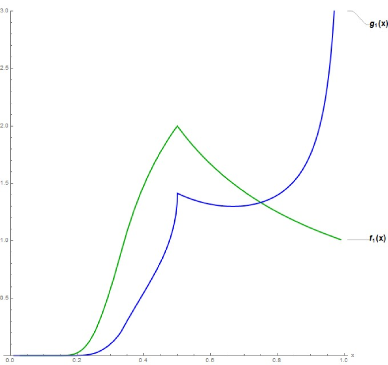
Figure 6: $f_{1}(x)=\dfrac{1}{x}\,\rho\left(\dfrac{1-x}{x}\right)$ and $g_{1}(x)=\dfrac{1}{2x^{3/2}}\sigma\left(\dfrac{1-x}{x}\right)$ comparison;the differential expression $g_{1}(x)=\dfrac{d}{dx}\left(\dfrac{1}{x^{1/2}}\sigma\left(\dfrac{1}{x}\right)\right)$ is akin to $f_{1}(x)=\dfrac{d}{dx}\,\rho\left(\dfrac{1}{x}\right)$.

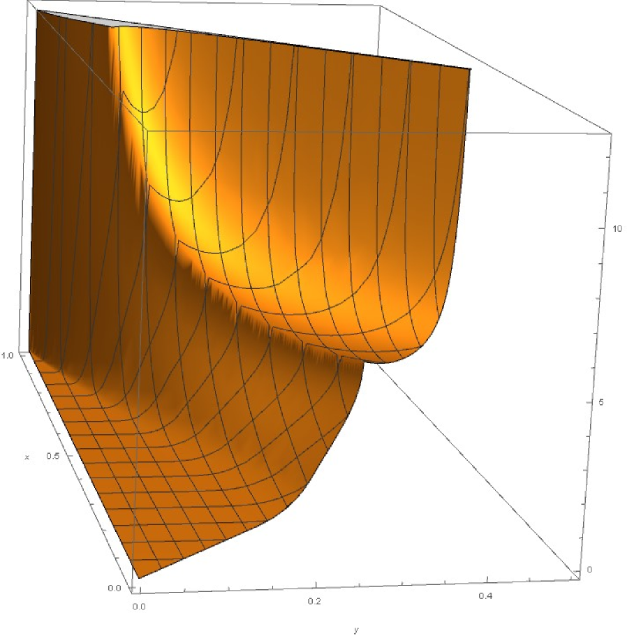
Figure 7: $g_{12}(x,y)=\dfrac{1}{4\,x\,y^{3/2}}\sigma\left(\dfrac{1-x-y}{y}\right)$ over $0\leq y\leq 1/2$ and $y\leq x\leq 1-y$; this contrasts sharply from plot of $f_{12}(x,y)$ in Figure 2 along diagonal segment $x=y$.

5 Addendum: Short Cycles

Given a random $n$-permutation, let $S_{r}$ denote the length of the $r^{\text{th}}$ shortest cycle ($0$ if the permutation has no $r^{\text{th}}$ cycle) and $C_{\ell}$ denote the number of cycles of length $\ell$.  Since, as $n\rightarrow\infty$, the distribution of $C_{\ell}$ approaches Poisson($1/\ell$) and $C_{1}$, $C_{2}$, $C_{3}$, … become asymptotically independent [29], we can calculate corresponding probabilities for $S_{r}$.  For example,

$$\mathbb{P}\left\{S_{1}=1\right\}=\mathbb{P}\left\{C_{1}\geq 1\right\}=1-\mathbb{P}\left\{C_{1}=0\right\}=1-e^{-1},$$

$$\mathbb{P}\left\{S_{1}=2\right\} =\mathbb{P}\left\{C_{1}=0\text{ \&\ }C_{2}\geq 1\right\}=\mathbb{P}\left\{C_{1}=0\right\}-\mathbb{P}\left\{C_{1}=0\text{ \&\ }C_{2}=0\right\}$$

$$=\mathbb{P}\left\{C_{1}=0\right\}\left(1-\mathbb{P}\left\{C_{2}=0\right\}\right)=e^{-1}\left(1-e^{-1/2}\right)=e^{-1}-e^{-3/2}$$

and, more generally,

$$\begin{array}[c]{ccc}\mathbb{P}\left\{S_{1}=i\right\}=e^{-H_{i-1}}-e^{-H_{i}},&&H_{m}={\displaystyle\sum\limits_{k=1}^{m}}\dfrac{1}{k}.\end{array}$$

It is understood that these are limiting quantities as $n\rightarrow\infty$.  As another example,

$$\mathbb{P}\left\{S_{2}=1\right\}=\mathbb{P}\left\{C_{1}\geq 2\right\}=1-\mathbb{P}\left\{C_{1}\leq 1\right\}=1-2e^{-1},$$

$$\mathbb{P}\left\{S_{2}=2\right\} =\mathbb{P}\left\{C_{1}=1\text{ \&\ }C_{2}\geq 1\right\}+\mathbb{P}\left\{C_{1}=0\text{ \&\ }C_{2}\geq 2\right\}$$

$$=\mathbb{P}\left\{C_{1}=1\right\}-\mathbb{P}\left\{C_{1}=1\text{ \&\ }C_{2}=0\right\}+\mathbb{P}\left\{C_{1}=0\right\}-\mathbb{P}\left\{C_{1}=0\text{ \&\ }C_{2}\leq 1\right\}$$

$$=e^{-1}\left(1-e^{-1/2}\right)+e^{-1}\left(1-\tfrac{3}{2}e^{-1/2}\right)=2e^{-1}-\tfrac{5}{2}e^{-3/2}$$

and

$$\mathbb{P}\left\{S_{2}=j\right\}=\left(H_{j-1}+1\right)e^{-H_{j-1}}-\left(H_{j}+1\right)e^{-H_{j}}.$$

Similar reasoning leads to

$$\mathbb{P}\left\{S_{1}=i\text{ \&\ }S_{2}=j\right\}=\left\{\begin{array}[c]{lll}e^{-H_{i-1}}-\left(1+\dfrac{1}{i}\right)e^{-H_{i}}&\vskip 12.0pt plus 4.0pt minus 4.0pt&\text{if }i=j,\\ \dfrac{1}{i}\left(e^{-H_{j-1}}-e^{-H_{j}}\right)&\vskip 12.0pt plus 4.0pt minus 4.0pt&\text{if }i<j,\\ 0&&\text{otherwise}\end{array}\right.$$

enabling a conjecture: $\mathbb{E}(S_{1}S_{2})=O(\ln(n)^{3})$.  A proof still remains out of reach.

6 Acknowledgements

I am grateful to Michael Rogers, Josef Meixner, Nicholas Pippenger, Eran Tromer, John Kingman, Andrew Barbour, Ross Maller and Joseph Blitzstein for helpful discussions.  The creators of Mathematica, as well as administrators of the MIT Engaging Cluster, earn my gratitude every day.  Interest in this subject has, for me, spanned many years [30, 31].  A sequel to this paper will be released soon [32].

References

- [1] S. R. Finch, Permute, Graph, Map, Derange, arXiv:2111.05720.
- [2] S. R. Finch, Rounds, Color, Parity, Squares, arXiv:2111.14487.
- [3] D. E. Knuth and L. Trabb Pardo, Analysis of a simple factorization algorithm, Theoret. Comput. Sci. 3 (1976) 321–348; also in Selected Papers on Analysis of Algorithms, CSLI, 2000, pp. 303-339; MR0498355.
- [4] S. R. Finch, Second best, Third worst, Fourth in line, arXiv:2202.07621.
- [5] P. Billingsley, On the distribution of large prime divisors, Period. Math. Hungar. 2 (1972) 283–289; MR0335462.
- [6] G. A. Watterson, The stationary distribution of the infinitely-many neutral alleles diffusion model, J. Appl. Probab. 13 (1976) 639–651; 14 (1977) 897; MR0504014 and MR0504015.
- [7] A. M. Vershik, Asymptotic distribution of factorizations of natural numbers into prime divisors (in Russian), Dokl. Akad. Nauk SSSR v. 289 (1986) n. 2, 269–272; Engl. transl. in Soviet Math. Dokl. v. 34 (1987) 57–61; MR0856456.
- [8] R. Arratia, A. D. Barbour and S. Tavaré, Random combinatorial structures and prime factorizations, Notices Amer. Math. Soc. 44 (1997) 903–910; MR1467654.
- [9] J. F. C. Kingman, Poisson processes revisited, Probab. Math. Statist. 26 (2006) 77–95; MR2301889.
- [10] L. A. Shepp and S. P. Lloyd, Ordered cycle lengths in a random permutation, Trans. Amer. Math. Soc. 121 (1966) 340–357; MR0195117.
- [11] R. Arratia, A. D. Barbour and S. Tavaré, Logarithmic Combinatorial Structures: a Probabilistic Approach, Europ. Math. Society, 2003, pp. 21-24, 52, 87–89, 118; MR2032426.
- [12] R. G. Pinsky, A view from the bridge spanning combinatorics and probability, arXiv:2105.13834.
- [13] R. C. Griffiths, On the distribution of allele frequencies in a diffusion model, Theoret. Population Biol. 15 (1979) 140–158; MR0528914.
- [14] T. Shi, Cycle lengths of -biased random permutations, B.S. thesis, Harvey Mudd College, 2014, http://scholarship.claremont.edu/hmc_theses/65/.
- [15] E. Bach and R. Peralta, Asymptotic semismoothness probabilities, Math. Comp. 65 (1996) 1701–1715; MR1370848.
- [16] R. Lambert, Computational Aspects of Discrete Logarithms, Ph.D. thesis, Univ. of Waterloo, 1996.
- [17] S. H. Cavallar, On the Number Field Sieve Integer Factorisation Algorithm, Ph.D. thesis, Univ. Leiden, 2002; ch. 2 also in The Three-Large-Primes Variant of the Number Field Sieve, CWI report MAS-R0219, 2002, http://ir.cwi.nl/pub/4222.
- [18] C. Zhang, An Extension of the Dickman Function and its Application, Ph.D. thesis, Purdue Univ., 2002; Distribution of -semismooth integers, PanAmer. Math. J. 18 (2008) 45–60; MR2467928.
- [19] W. H. Ekkelkamp, The role of semismooth numbers in factoring large numbers, Proc. Conf. on Algorithmic Number Theory, ed. A.-M. Ernvall-Hytönen, M. Jutila, J. Karhumäki and A. Lepistö, Turku Centre for Computer Science, 2007, pp. 40–44; http://oldtucs.abo.fi/publications/.
- [20] W. H. Ekkelkamp, On the Amount of Sieving in Factorization Methods, Ph.D. thesis, Univ. Leiden, 2010; http://www.universiteitleiden.nl/en/research/research-output/.
- [21] E. Bach and J. Sorenson, Approximately counting semismooth integers, Proc. 38th Internat. Symp. on Symbolic and Algebraic Computation (ISSAC), ACM, 2013, pp. 23–30; arXiv:1301.5293; MR3206336.
- [22] E. H. Cliffe, Reflections on the Number Field Sieve, Ph.D. thesis, Univ. of Bath, 2007; http://researchportal.bath.ac.uk/en/studentTheses/.
- [23] E. Tromer, Hardware-Based Cryptanalysis, Ph.D. thesis, Weizmann Institute of Science, 2007; http://www.cs.tau.ac.il/~tromer/phd-dissertation/.
- [24] A. Granville, The anatomy of integers and permutations, unpublished note, 2008, http://dms.umontreal.ca/~andrew/PDF/Anatomy.pdf.
- [25] A. Granville, J. Granville and R. J. Lewis, Prime Suspects. The Anatomy of Integers and Permutations, Princeton Univ. Press, 2019, pp. 200–201; MR3966460.
- [26] S. P. Lloyd, Ordered prime divisors of a random integer, Annals of Probab. 12 (1984) 1205–1212; MR0757777.
- [27] J. F. C. Kingman, The Poisson-Dirichlet distribution and the frequency of large prime divisors, unpublished note, 2004, http://www.newton.ac.uk/documents/preprints/.
- [28] T. Tao, Cycles of a random permutation, and irreducible factors of a random polynomial, unpublished note, 2015, http://terrytao.wordpress.com/2015/07/15/.
- [29] R. Arratia and S. Tavaré, The cycle structure of random permutations, Annals of Probab. 20 (1992) 1567–1591; MR1175278.
- [30] S. R. Finch, Golomb-Dickman constant, Mathematical Constants, Cambridge Univ. Press, 2003, pp. 284–292; MR2003519.
- [31] S. R. Finch, Extreme prime factors, Mathematical Constants II, Cambridge Univ. Press, 2019, pp. 171–172; MR3887550.
-
[32]
S. R. Finch, Components and cycles of random mappings,
forthcoming.
Steven Finch MIT Sloan School of Management Cambridge, MA, USA steven_finch@harvard.edu