Hierarchical Path-planning from Speech Instructions with
Spatial Concept-based Topometric Semantic Mapping

Abstract

Navigating to destinations using human speech instructions is essential for autonomous mobile robots operating in the real world. Although robots can take different paths toward the same goal, the shortest path is not always optimal. A desired approach is to flexibly accommodate waypoint specifications, planning a better alternative path, even with detours. Furthermore, robots require real-time inference capabilities. Spatial representations include semantic, topological, and metric levels, each capturing different aspects of the environment. This study aims to realize a hierarchical spatial representation by a topometric semantic map and path planning with speech instructions, including waypoints. We propose SpCoTMHP, a hierarchical path-planning method that utilizes multimodal spatial concepts, incorporating place connectivity. This approach provides a novel integrated probabilistic generative model and fast approximate inference, with interaction among the hierarchy levels. A formulation based on control as probabilistic inference theoretically supports the proposed path planning. Navigation experiments using speech instruction with a waypoint demonstrated the performance improvement of path planning, WN-SPL by 0.589, and reduced computation time by 7.14 sec compared to conventional methods. Hierarchical spatial representations offer a mutually understandable form for humans and robots, enabling language-based navigation tasks.

I Introduction

Autonomous robots need to accomplish linguistic interaction tasks, such as navigation, to coexist with humans in the real world. To fulfill this task, the robot must adaptively form spatial structures and place semantics from the multimodal observations obtained while moving in the environment [1, 2]. Topometric semantic maps are helpful for path planning using the generalized units of place, human-robot linguistic interaction, and robot support for humans. A major challenge is the efficient construction and utilization of these hierarchical spatial representations by robots for interaction tasks. The main purpose of this study was to realize efficient spatial representations and high-speed path planning from human speech instructions specifying waypoints using topological semantic maps incorporating place connectivity.

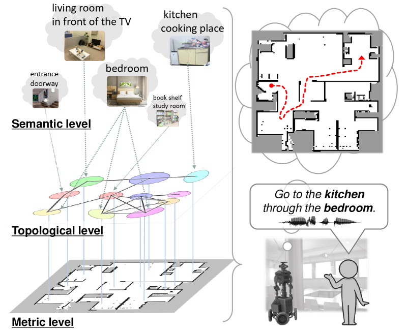
Figure 1: Overview. Left: Hierarchy of spatial representation with topometric semantic mapping; Right: Path planning from spoken instruction with waypoint and goal specifications.

While the shortest path may not always be optimal, robots can choose alternative paths to avoid certain areas or perform specific tasks. For example, the robot will take a different route to reach a goal to avoid the living room with the guests or to check on the pets in the bedroom. Thus, users can guide the robot toward an improved path by specifying waypoints.

Hierarchical spatial representations provide a mutually understandable form for humans and robots to render language-based navigation tasks feasible. As shown in Fig. 1, this study deals with the three levels of spatial representation: (i) the semantic level, which represents place categories associated with words and abstracted by multimodal observations; (ii) the topological level, which represents the adjacency of places in a graph structure; (iii) the metric level, which represents the occupancy grid map and is obtained by simultaneous localization and mapping (SLAM) [3]. This study defines semantic-topological knowledge as spatial concepts.

This study had two phases: spatial concept learning and path planning. In the learning phase, a robot moves around the environment with a person. Then, the person speaks a natural language, teaching utterances about the location, such as “This is a dining room.” In the planning phase, the robot observes speech instructions, such as “go to the kitchen” as a basic task and “go to the kitchen through the bedroom” as an advanced task. In particular, this study focused on hierarchical path planning in advanced tasks.

We propose a spatial concept-based topometric semantic mapping for hierarchical path planning (SpCoTMHP) with a probabilistic generative model. The topometric semantic map enables path planning that combines abstracted place transitions and geometrical structures in the environment. We also developed approximate inference methods for effective path planning, where each hierarchy level can influence the others. The proposed path planning is theoretically supported based on control as probabilistic inference (CaI) [4]. The CaI bridged the theoretical gap between the probabilistic inference and the control problems, including reinforcement learning. The main contributions of this work are as follows:

1. We demonstrate that the integrated model can autonomously construct hierarchical spatial representations, including place connectivity, from the robot’s multimodal observations, leading to improved performance in learning and planning.

2. We show that approximate inference based on CaI enables real-time planning of efficient and adaptive paths from waypoint and goal candidates.

II Related Work

II-A Topometric semantic map

Research on semantic mapping has been increasingly emphasized in recent years; semantic mapping assigns place meanings to a robot’s map [1, 2]. However, many existing studies provide a preset location label for an area on a map. Our approach allows unsupervised learning based on multimodal perceptual information for categorizing unknown places and flexible vocabulary assignments.

The use of topological structures enables more accurate semantic mapping [5]. Our method is also expected to improve its performance by introducing topological levels. The nodes in a topological map can vary depending on the method, such as room units or small regions [6, 7]. Kimera [8] used multiple levels of spatial hierarchical representation, such as metrics, rooms, places, semantic levels, objects, and agents. In our study, the robot automatically determined the spatial segmentation unit based on experience.

Some semantic mapping studies [9, 10] have successfully constructed topological semantic maps from visual images or metric maps using convolutional neural networks. However, these studies did not consider path planning. By contrast, our method is characterized by an integrated model inclusive of learning and planning.

II-B Hierarchical path planning

Hierarchical path planning has long been a topic of study, as in hierarchical A^⋆ [11]. Using topological maps for path planning (including learning paths between edges) is more effective for reducing computational complexity than considering only the movement between cells in a metric map [6, 12, 8]. In addition, the extension to semantic maps enables navigation based on speech [13].

Because our method realizes a hierarchy based on the CaI framework [4], it is theoretically connected with hierarchical reinforcement learning. In hierarchical reinforcement learning, sub-goals and policies are autonomously estimated [14, 15]. In our study, tasks similar to hierarchical reinforcement learning were realized to infer probabilistic models. In addition, recent studies on vision-and-language navigation have used deep and reinforcement learning [16, 17]. The proposed probabilistic model autonomously navigates toward the target location using speech instructions as a modality.

III Preliminary: SpCoSLAM and SpCoNavi

SpCoSLAM [18] forms spatial concept-based semantic maps based on multimodal observations obtained from the environment. SpCoSLAM can acquire novel place categories and vocabularies from unknown environments. However, SpCoSLAM has been unable to estimate a topological level, that is, whether one place is spatially connected to another. In this study, we applied the hidden semi-Markov model (HSMM) [19], which estimates the transition probabilities between places and constructs a topological graph, instead of the Gaussian mixture model (GMM) part in SpCoSLAM.

In addition, SpCoNavi [20] plans the path in the CaI framework [4], which focuses on the action decision in the probabilistic generative model of SpCoSLAM. SpCoNavi has realized navigation from simple speech instructions using a spatial concept acquired autonomously by the robot. However, SpCoNavi is not hierarchical path planning, and situations specifying a waypoint are not conducted. In addition, there are several problems to be solved: SpCoNavi, based on the Viterbi algorithm [21], is computationally expensive because all grids of the occupied grid map are used as the state space, and it is vulnerable to the real-time performance required for robot navigation. SpCoNavi, based on the A^⋆ approximation, reduces the computational cost, but its performance is inferior to that of the Viterbi. Therefore, in this study, we utilized a topological semantic map based on spatial concepts to reduce the number of states and rapidly infer possible paths between each state.

IV Proposed Method: SpCoTMHP

We propose a spatial concept-based topometric semantic mapping for hierarchical path planning (SpCoTMHP). The proposed method realizes efficient navigation from human speech instructions through inference based on a probabilistic generative model. Our approach enhances human comprehensibility and explainability by employing Gaussian distributions as the fundamental spatial units. The capabilities of the proposed generative model are as follows: (i) Place categorization by extracting connection relations between places using unsupervised learning; (ii) Many-to-many correspondence between words and places; and (iii) Efficient hierarchical path planning by introducing two variables with different time constants.

IV-A Definition of probabilistic generative model

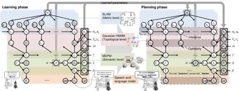
Figure 2: Graphical model representation of SpCoTMHP; (left) spatial concept learning; (right) path planning. The two phases imply different probabilistic inferences for the same generative model. The graphical model represents the conditional dependency between random variables. Gray nodes indicate observations or learned parameters as fixed conditional variables. White nodes denote unobserved latent variables to be estimated. Arrows from the global variables to local variables other than $T$ and $E$ are omitted.

SpCoTMHP is designed as an integrated model for each module: SLAM, HSMM, multimodal Dirichlet process mixture (MDPM) for place categorization, and the speech-and-language model. The integrated model has the advantage that the inference works as a whole, complementing each uncertainty. Figure 2 shows the graphical model representation of SpCoTMHP, and Table I lists each variable of the graphical model. Unlike SpCoSLAM [18], SpCoTMHP introduces two different time units and extends GMM to HSMM. The definition of the generative process represented by the graphical model of SpCoTMHP is as follows.

SLAM part: Eq. (1) represents the measurement model, and Eq. (2) represents a motion model that is a state-transition related to the position in SLAM as follows:

$$z_{t} \sim p(z_{t}\mid x_{t},m), t =1,2,\dots,T$$ (1)

$$x_{t} \sim p(x_{t}\mid x_{t-1},u_{t}).$$ (2)

Self-localization assumes a transition at time $t$ owing to the robot’s motion.

HSMM part: The HSMM connects two units: time $t$ and event $e$. A binary random variable that indicates whether there is an event is defined as

$$o_{t} \sim p(o_{t}\mid x_{t},i_{e},D_{e},\mu,\Sigma)={\cal N}(x_{t}\mid\mu_{i_{e}},\Sigma_{i_{e}}), \text{if $o_{t}=1$},$$ (3)

where $\mu=\{\mu_{k}\}$, $\Sigma=\{\Sigma_{k}\}$, and $o_{t}=1$ denotes that the event occurred at time $t$. This event-driven variable corresponds to the optimality variable in the CaI [4]. The duration distribution assumes uniform distribution in $[1,T]$:

$$D_{e} \sim{\rm Unif}(1,T), e =1,2,\dots,E$$ (4)

where the equation relating $t$ and $e$ is $t_{e}=\sum_{e^{\prime}<e}D_{e^{\prime}}$, and the final time at the event $e$ is $t^{\prime}_{e}=t_{e}+D_{e}-1$. Thus, $E\leqq T$ and $T=\sum_{e=1}^{E}D_{e}$.
The position distribution represents a coherent unit of place and is represented by a Gaussian distribution. To capture transitions between places, $\psi_{k}$ is introduced as follows:

$$\mu_{k} \sim{\cal N}(m_{0},\Sigma_{k}/\kappa_{0}), k =1,2,\dots,\infty$$ (5)

$$\Sigma_{k} \sim{\cal IW}(V_{0},\nu_{0}),$$ (6)

$$\psi_{k} \sim{\rm DP}(\omega),$$ (7)

where ${\cal N}()$ is a multivariate Gaussian distribution, ${\cal IW()}$ is the inverse-Wishart distribution, and ${\rm DP()}$ represents the Dirichlet process. See the literature on machine learning [22] for the specific formulas of these probability distributions.

HSMM + MDPM connection: The probability distribution of $i_{e}$ for connecting two modules is defined by unigram rescaling (UR) [23] as follows:

$$i_{e} \sim p(i_{e}\mid{i_{e-1}},\psi,{C_{e}},\phi)$$ (8)

$$\quad\overset{\mathrm{UR}}{\approx}{\rm Mult}(i_{e}\mid\psi_{i_{e-1}})\frac{{\rm Mult}(i_{e}\mid\phi_{C_{e}})}{\sum_{c^{\prime}=1}^{L}{\rm Mult}(i_{e}\mid\phi_{c^{\prime}})},$$ (9)

where $\psi=\{\psi_{k}\}$, $\phi=\{\phi_{l}\}$, and ${\rm Mult()}$ is a multinomial distribution.

MDPM part: The MDPM is positioned at the semantic level, representing spatial concepts based on places $i_{e}$, speech-language $S_{e}$, and image features $f_{e}$ as follows:

$$\pi \sim{\rm DP}(\alpha),$$ (10)

$$\phi_{l} \sim{\rm DP}(\gamma), l =1,2,\dots,\infty$$ (11)

$$\theta_{l} \sim{\rm Dir}(\chi),$$ (12)

$$W_{l} \sim{\rm Dir}(\beta),$$ (13)

$$C_{e} \sim{\rm Mult}(\pi), e =1,2,\dots,E$$ (14)

$$f_{e} \sim{\rm Mult}(\theta_{C_{e}}),$$ (15)

where ${\rm Dir()}$ is the Dirichlet distribution. According to the data, the DP automatically determines the numbers of spatial concepts $L$ and position distributions $K$.

MDPM + language model connection: The probability distribution of $S_{e}$ for connecting two modules is defined by UR [23] as follows:

$$S_{e} \sim p(S_{e}\mid C_{e},W,LM)$$ (16)

$$\quad\overset{\mathrm{UR}}{\approx}p(S_{e}\mid LM)\prod_{b=1}^{B_{e}}\frac{{\rm Mult}(S_{e,b}\mid W_{C_{e}})}{\sum_{c^{\prime}=1}^{L}{\rm Mult}(S_{e,b}\mid W_{c^{\prime}})},$$ (17)

where $W=\{W_{l}\}$. $B_{e}$ is the number of words in the sentence, and $S_{e,b}$ is the $b$-th word in the sentence at event $e$.

Speech-and-language model part: The generative process as the likelihood of speech given a word sequence is shown as follows:

$$y_{e} \sim p(y_{e}\mid S_{e},AM).$$ (18)

TABLE I: Description of the random variables used in our model

Symbol	Definition
$m$	Environmental map (occupancy grid map)
$x_{t}$	Self-position of the robot (state variable)
$u_{t}$	Control data (action variable)
$z_{t}$	Depth sensor data
$o_{t}$	Optimality variable (event-driven)
$D_{e}$	Duration length for $o_{t}$ in $i_{e}$
$i_{e}\in\{k\}$	Category index of the position distributions
$C_{e}\in\{l\}$	Category index of spatial concepts
$f_{e}$	Visual features of the camera image
$y_{e}$	Speech signal of the uttered sentence
$S_{e}$	Word sequence in the uttered sentence
$\mu_{k}$, $\Sigma_{k}$	Parameters of multivariate Gaussian distribution    (position distribution)
$\psi_{k}$	Parameter of state-transition for $i_{e}$ in $i_{e-1}=k$
$\pi$	Parameter of mixture weights for $C_{e}$
$\phi_{l}$	Parameter of mixture weights for $i_{e}$ in $C_{e}=l$
$\theta_{l}$	Parameter of feature distribution for $f_{e}$
$W_{l}$	Parameter of word distribution for $S_{e}$
$LM$	Language model (n-gram and word dictionary)
$AM$	Acoustic model for speech recognition
$\alpha$, $\beta$, $\gamma$, $\chi$, $\omega$,	Hyperparameters of prior distributions
$m_{0}$, $\kappa_{0}$, $V_{0}$, $\nu_{0}$
$T$	Final time the robot operated
$E$	Total number of user utterances (in the learning) or total number of location moves (in the planning)
$L$	Total number of spatial concepts
$K$	Total number of position distributions

IV-B Spatial concept learning as topometric semantic mapping

The joint posterior distribution is described as

$$p(x_{0:T},S_{1:E},\mathbf{C}_{1:E},\mathbf{\Theta}\mid u_{1:T},z_{1:T},o^{\ast}_{t^{\prime}_{1:E}},y_{1:E},f_{1:E},\mathbf{h}),$$ (19)

where the set of latent variables is denoted by $\mathbf{C}_{1:E}=\{i_{1:E},C_{1:E}\}$, the set of global model parameters $\mathbf{\Theta}=\{m,\mu,\Sigma,\psi,\pi,\phi,\theta,W,LM,AM\}$, and the set of hyperparameters $\mathbf{h}=\{\alpha,\beta,\gamma,\chi,\omega,m_{0},\kappa_{0},V_{0},\nu_{0}\}$. The set of event-driven variables is $o^{\ast}_{t^{\prime}_{1:E}}=\{o_{t^{\prime}_{e}}=1\}^{E}_{e=1}$.

In this paper, as an approximation to sampling from Eq. (19), the parameters are estimated as follows:

$$x_{0:T},m \sim p(x_{0:T},m\mid u_{1:T},z_{1:T}),$$ (20)

$$S_{e} \sim p(S_{e}\mid y_{e},LM,AM),\quad e=1,2,\dots,E$$ (21)

$$\mathbf{C}_{1:E},\mathbf{\Theta}^{\prime} \sim p(\mathbf{C}_{1:E},\mathbf{\Theta}^{\prime}\mid x_{0:T},o^{\ast}_{t^{\prime}_{1:E}},S_{1:E},f_{1:E},\mathbf{h}),$$ (22)

where $\mathbf{\Theta}^{\prime}=\{\mu,\Sigma,\psi,\pi,\phi,\theta,W\}$. Eq. (20) is realized by grid-based FastSLAM 2.0 [3]. Eq. (21) represents speech recognition of $y_{e}$. $LM$ and $AM$ were pre-set. The proposed method can deal with uncertainty in speech recognition by capturing the $N$-best speech recognition results as a Monte Carlo approximation. The variables in Eq. (22) can be learned using Gibbs sampling, a Markov chain Monte-Carlo-based batch learning algorithm, specifically, the weak-limit and direct-assignment sampler [19].

In the learning phase, the user gives a teaching utterance each time the robot transitions between locations. Because the utterance is event-driven, it is assumed that the variables on the spatial concepts are observed only at event $e$. Here, the time of the $e$-th event (when the robot observes an utterance indicates the place) is $t^{\prime}_{e}$. In other words, $o_{t^{\prime}_{e}}=1$ is observed at times $t^{\prime}_{e}$, and $o_{t}$ is unobserved at other times. Therefore, the inference for learning $i_{e}$ is equivalent to an HMM.

Reverse replay: In the case of spatial movement, we can transition from $i_{e-1}$ to $i_{e}$ and vice versa. Therefore, $i^{\prime}_{E:1}$, which is replayed using the steps of $e$ in reverse order, can also be used for learning when sampling $\psi$. This was inspired by the replay performed in the hippocampus of the brain [24].

IV-C Hierarchical path planning by control as inference

The probabilistic distribution, representing trajectory $\tau=\{u_{1:T},x_{1:T}\}$ when a speech instruction $y_{e}$ is given, is maximized to estimate an action sequence $u_{1:T}$ (and the path $x_{1:T}$ on the map) as follows:

$$u_{1:T} = \operatorname*{argmax}_{u_{1:T}}p(\tau\mid o^{\ast}_{1:T},y_{1:E},x_{0},\mathbf{\Theta}).$$ (23)

The planning horizon at metric level $T$ is the final time of the entire task when one time-step traverses one grid block on the metric map. The planning horizon at topological level $E$ is the number of event steps in navigating by speech instruction. As shown in Eqs. (3) and (4), each event step $e$ corresponds to time series ${t_{e}:t^{\prime}_{e}}$. The metric-level planning horizon in step $e$ corresponds to the duration $D_{e}$ of the HSMM. In the metric-level planning horizon, the event-driven variable is always $o^{\ast}_{1:T}=\{o_{t}=1\}_{t=1}^{T}$ by the CaI. Speech instruction $y_{e}$ is assumed to be the same as that from $e=1$ to $E$. This means that $o_{t}$ and $y_{e}$ are multiple optimalities in terms of CaI [25]. From the above, Eq. (23) is as follows:

$$p(\tau\mid o^{\ast}_{1:T},y_{1:E},x_{0},\mathbf{\Theta})$$

$$\approx\prod_{e=1}^{E}\left[\sum_{i_{e}=1}^{K}\frac{{\rm Mult}(i_{e}\mid\psi_{i_{e-1}})}{\sum_{c^{\prime}=1}^{L}{\rm Mult}(i_{e}\mid\phi_{c^{\prime}})}\right.$$

$$\quad\sum_{{C}_{e}=1}^{L}{\rm Mult}(i_{e}\mid\phi_{C_{e}}){\rm Mult}(S_{e}\mid W_{C_{e}}){\rm Mult}(C_{e}\mid\pi)$$

$$\quad\left.\prod_{t=t_{e}}^{t^{\prime}_{e}}{{\cal N}(x_{t}\mid\mu_{i_{e}},\Sigma_{i_{e}})}p(x_{t}\mid m)p(x_{t}\mid x_{t-1},u_{e})\right],$$ (24)

$$S_{e}\sim p(S_{e}\mid y_{e},LM,AM),$$ (25)

where $p(x_{t}\mid m)$ is a probabilistic representation of the cost map, and the maximum limit value of $D_{1:E}$ is given. In addition, the word sequence $S_{e}$ is obtained by speech recognition of $y_{e}$ as $N$-best’s bag-of-words. The assumptions, for example, the SLAM models and cost map, in the derivation of the equation are the same as those in SpCoNavi’s paper [20].

In this study, we assumed that the robot could extract words that indicate the goal and waypoint from a particular utterance sentence. In topological-level planning, including the waypoint, the waypoint word is input in the first half and the target word in the second half.

IV-D Approximate inference for hierarchical path planning

The strict inference of Eq. (24) requires a double-forward backward calculation. In this case, it is necessary to reduce the calculation cost to accelerate path planning, which is one of the purposes of this study. Therefore, we propose an algorithm to solve Eq. (24): Algorithm 1 shows the hierarchical planning algorithm produced by SpCoTMHP.

Path planning is divided into topological and metric levels, and the CaI is solved at each level. Metric-level planning assumes that the partial paths in each transition between places are solved in A^⋆. The partial paths can be precomputed regardless of the speech instruction. Topological-level planning is approximated concerning the probability distribution of $i_{e}$, assuming Markov transitions. Finally, the partial paths in each transition between places are integrated as a whole path. Metric and topological planning can influence each other.

Algorithm 1 Hierarchical path planning algorithm.

1:// Pre-calculation:

2:$\{\hat{x}_{t^{\prime}_{e}|i_{e}}\}\sim\mathtt{Gaussian\_Mixture}(\mathbf{\phi},\mathbf{\mu},\mathbf{\Sigma})$

3:Create a graph between waypoint candidates

4:for all nodes, $n_{i_{e-1}}\rightarrow n_{i_{e}}$, do

5:     $\hat{\mathbf{x}}_{i_{e-1},i_{e}}^{[n_{i_{e-1}},n_{i_{e}}]}\leftarrow{\rm A}^{\star}(\hat{x}_{t^{\prime}_{e-1}|i_{e-1}}^{[n_{i_{e-1}}]},\hat{x}_{t^{\prime}_{e}|i_{e}}^{[n_{i_{e}}]},w_{e})$

6:     Calculate likelihood $\hat{\mathbf{w}}_{i_{e-1},i_{e}}^{[n_{i_{e-1}},n_{i_{e}}]}$ for partial paths

7:end for

8:// When a speech instruction $y_{e}$ is given:

9:$S_{e}\leftarrow\mathtt{Speech\_Recognition}(y_{e},LM,AM)$

10:Estimate an index $i_{0}$ of the place in initial position $x_{0}$

11:$\mathbf{n}_{1:E},i_{1:E}\leftarrow\mathtt{Search}(i_{0},S_{e},\hat{\mathbf{w}},\mathbf{\Theta})$ // Eq. (28)

12:Connect the partial paths $\mathbf{n}_{1:E}$ as the whole path $\mathbf{x}_{1:E}$

13:$\mathbf{x}_{1:E}\leftarrow\mathtt{Path\_Smoothing}(\mathbf{x}_{1:E},m)$ // optional process

Path planning at the metric level (i.e., partial path $\mathbf{x}_{i_{e-1},i_{e}}$ when transitioning from $i_{e-1}$ to $i_{e}$) is described as follows:

$$x_{t_{e}:t^{\prime}_{e}} =\operatorname*{argmax}_{x_{t_{e}:t^{\prime}_{e}}}\prod_{t=t_{e}}^{t^{\prime}_{e}}{{\cal N}(x_{t}\mid\mu_{i_{e}},\Sigma_{i_{e}})}$$

$$\qquad\qquad\qquad p(x_{t}\mid m)p(x_{t}\mid x_{t-1},u_{e}).$$ (26)

This means that the inference of a metric-level path can be expressed in terms of CaI.

Calculating Eq. (24) for all possible positions was difficult. Therefore, we used the mean or sampled values from the Gaussian mixture of position distributions as a goal position candidate, that is, $\hat{x}_{t^{\prime}_{e}|i_{e}}^{[n_{i_{e}}]}\sim{\cal N}(x_{t}|\mu_{i_{e}},\Sigma_{i_{e}})$. In this case, $n_{i_{e}}$ is an index that takes values of up to $N_{i_{e}}$, which is the number of candidate points sampled for a specific $i_{e}$. By sampling multiple points according to the Gaussian distribution, candidate waypoints that follow the rough shape of the place can be selected. For example, it does not necessarily have to go to the center of a long corridor.

Therefore, as a concrete solution to Eq. (26), the partial path in the transition of candidate points from place $i_{e-1}$ to place $i_{e}$ is estimated as

$$\hat{\mathbf{x}}_{i_{e-1},i_{e}}^{[n_{i_{e-1}},n_{i_{e}}]} ={\rm A}^{\star}(\hat{x}_{t^{\prime}_{e-1}|i_{e-1}}^{[n_{i_{e-1}}]},\hat{x}_{t^{\prime}_{e}|i_{e}}^{[n_{i_{e}}]},w_{e}),$$ (27)

where ${\rm A}^{\star}(s,g,w_{e})$ denotes the function of the A^⋆ search algorithm, the initial position is $s$, the goal position is $g$, and the cost function is $w_{e}={\cal N}(x_{t}|\mu_{i_{e}},\Sigma_{i_{e}})p(x_{t}|m)$. The estimated partial path length can be interpreted as the estimated value of $D_{e}$.

The selection of a series of partial metric path candidates corresponds to the selection of the entire path. Thus, we can replace the formulation of the maximization problem. Each partial metric path has corresponding indices $i_{e-1}$ and $i_{e}$. Therefore, given a series of index pairs representing transitions between position distributions, the candidate paths to be considered are naturally narrowed down to a series of corresponding partial paths. The series of candidate indices that determines the series of candidate paths, in this case, is $\mathbf{n}_{1:E}=(n_{i_{0}},n_{i_{1}},\dots,n_{i_{E}})$. This partial path sequence can be regarded as a sampling approximation of $x_{1:T}$.

By taking the maximum value instead of summing for $i_{1:E}$, path planning at the topological level is described as

$$\mathbf{n}_{1:E},i_{1:E}=\operatorname*{argmax}_{\mathbf{n}_{1:E},i_{1:E}}\prod_{e=1}^{E}\frac{{\rm Mult}(i_{e}\mid\psi_{i_{e-1}})}{\sum_{c^{\prime}=1}^{L}{\rm Mult}(i_{e}\mid\phi_{c^{\prime}})}\hat{\mathbf{w}}_{i_{e-1},i_{e}}^{[n_{i_{e-1}},n_{i_{e}}]}$$

$$\sum_{{C}_{e}=1}^{L}{\rm Mult}(i_{e}\mid\phi_{C_{e}}){\rm Mult}(S_{e}\mid W_{C_{e}}){\rm Mult}(C_{e}\mid\pi),,$$ (28)

where $\hat{\mathbf{w}}_{i_{e-1},i_{e}}^{[n_{i_{e-1}},n_{i_{e}}]}$ is the likelihood of the metric path $\hat{\mathbf{x}}_{i_{e-1},i_{e}}^{[n_{i_{e-1}},n_{i_{e}}]}$ when transitioning from a candidate point of place $i_{e-1}$ to a candidate point of place $i_{e}$ at step $e$. In this case, it is equivalent to formulating the state variables in the distribution for the CaI as $\mathbf{x}_{1:E}$ and $i_{1:E}$. Therefore, path planning at the topological level can be expressed as CaI at event step $e$.

V Experiment I: Planning tasks in simulator

We experimented with path planning using spatial concepts, including topological structures from human speech instructions. We show that the proposed method can improve the efficiency of path planning. The simulator environment was SIGVerse, version 3.0 [26]. The virtual robot model in SIGVerse is the Toyota Human Support Robot (HSR). We used five three-bedroom home environments with different layouts and room sizes.

V-A Spatial concept-based topometric semantic map

There were 11 spatial concepts and position distributions for each environment. Fifteen training data samples were provided for each location. The SLAM and speech recognition modules were inferred individually by splitting from the model; that is, the self-location $x_{1:E}$ and word sequence $S_{1:E}$ were input into the model as observations. An environment map was generated by the gmapping package, which implements grid-based FastSLAM 2.0 [3], in the robot operating system (ROS). A word dictionary was provided in advance. We assumed that the speech recognition result was obtained accurately. Model parameters for the spatial concept were obtained via sampling from conditional distribution. We adopted the ideal learning results of spatial concepts; the latent variables $C_{t}$ and $i_{t}$ were accurately obtained. Figure 3 shows an example of the spatial concepts.

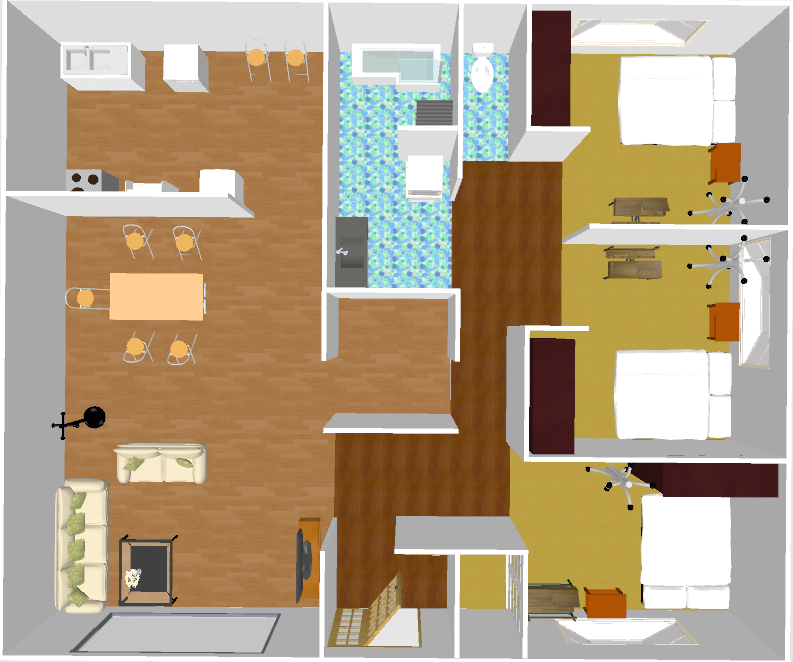
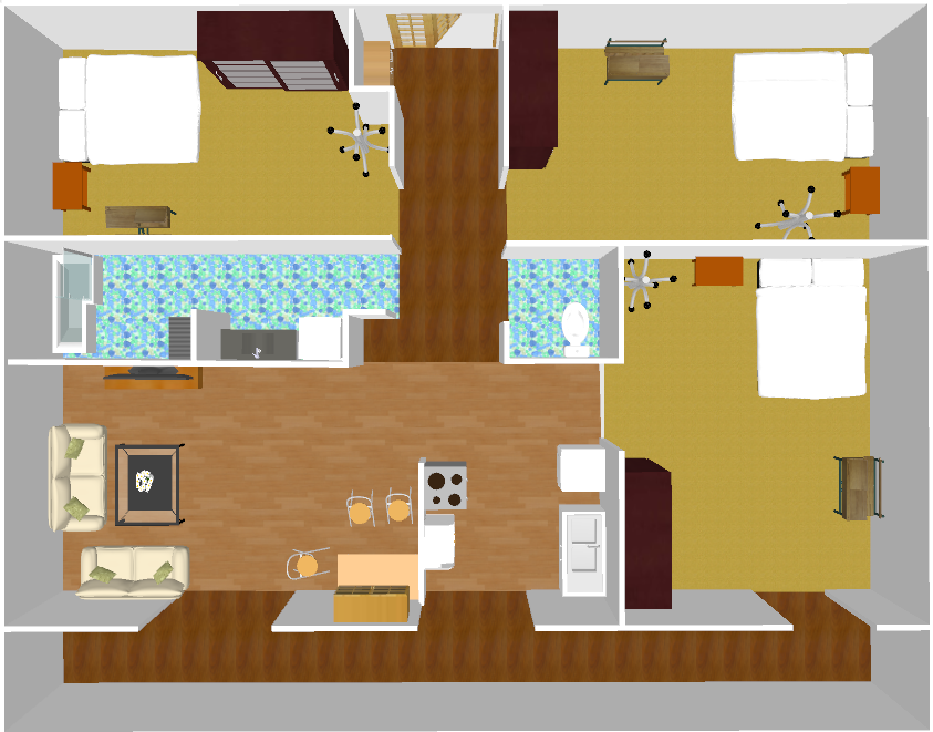
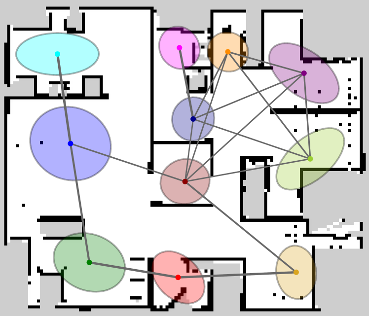
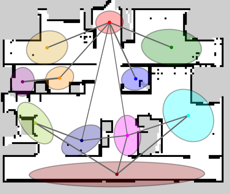
Figure 3: Overhead view of the simulator environments and the spatial concepts expressed by SpCoTMHP on the map (Experiments I). The colors were randomly set. If $(\psi_{k_{1},k_{2}}+\psi_{k_{1},k_{2}})/2>1/K$, then the centers $\mu_{k_{1}},\mu_{k_{2}}$ of Gaussian distributions are connected by an edge.

V-B Path planning from speech instructions

Two types of path-planning tasks were performed in the experiment.
Basic task: The robot obtained the word that identifies the target location as the instruction, such as “Go to the bedroom.”
Advanced task: The robot obtained the words that identify the waypoint locations and target as the speech instruction, such as “Go to the bedroom via the corridor.” We inputted both the waypoint and target words as bag-of-words into SpCoNavi, as the task was not demonstrated in the previous work [20].

We compared the performances of the methods as follows:

1. A^⋆ (goal estimated by spatial concepts): The goal position was obtained as $x^{\ast}\sim p(x\mid S^{\ast},\Theta)$ in SpCoSLAM, using the speech recognition result $S^{\ast}$.

2. SpCoSLAM [18] + SpCoNavi [20] (Viterbi [21])

3. SpCoSLAM [18] + SpCoNavi [20] (A^⋆ approx.)

4. Hierarchical path planning (HPP) without CaI, similar to [27]: Goal node is estimated by $i_{e}\sim p(i_{e}\mid S^{\ast},\mathbf{\Theta})$. The topological planning uses heuristic costs: (I) the cumulative cost, (II) the distance of partial paths in A^⋆.

5. SpCoTMHP (Topological: Dijkstra, Metric: A^⋆)

The evaluation metrics for path planning are the success weighted by path length (SPL) [28] when the robot reaches the target location and calculation runtime seconds (Time). N-SPL is the weighted success rate at which the robot reaches the closest target from the initial position when several places have the same name. W-SPL is the weighted success rate at which the robot passed the correct waypoints. WN-SPL is the weighted success rate at which the robot reaches the closest target and passes the correct waypoints.

Condition: The planning horizons were $E=10$ for the topological level and $D=100$ as the maximum limit value for the metric level in the SpCoTMHP. The number of position candidates in the sample was $N_{i_{e}}=1$. The proposed method subjected paths to moving average smoothing with a window size of 5. The planning horizon of SpCoNavi was $T=200$. The number of goal candidates of SpCoNavi (A^⋆ approx.) was $J=10$. The global cost map was obtained from the costmap_2d package in the ROS. The robot’s initial position was set from arbitrary movable coordinates on the map. The user provided a word to indicate the target’s name. The state of self-position $x_{t}$ is expressed discretely for each movable cell in the occupancy grid map $m$. The motion model assumes a deterministic model. The control value $u_{t}$ assumes to move one cell on the map per time-step. Action $u_{t}$ is discretized into $\mathcal{A}=$ {stay, up, down, left, right}. This study was implemented using Python on one CPU, an Intel Core i7-6850K, with 16GB DDR4 2133MHz SDRAM.

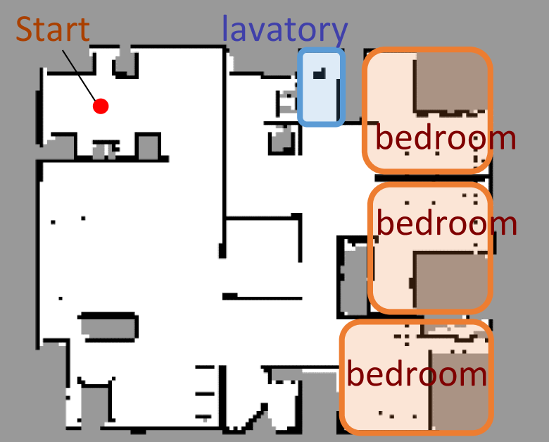
(a) Situation

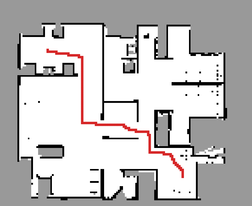
(b) SpCoNavi (A^⋆ approx.)

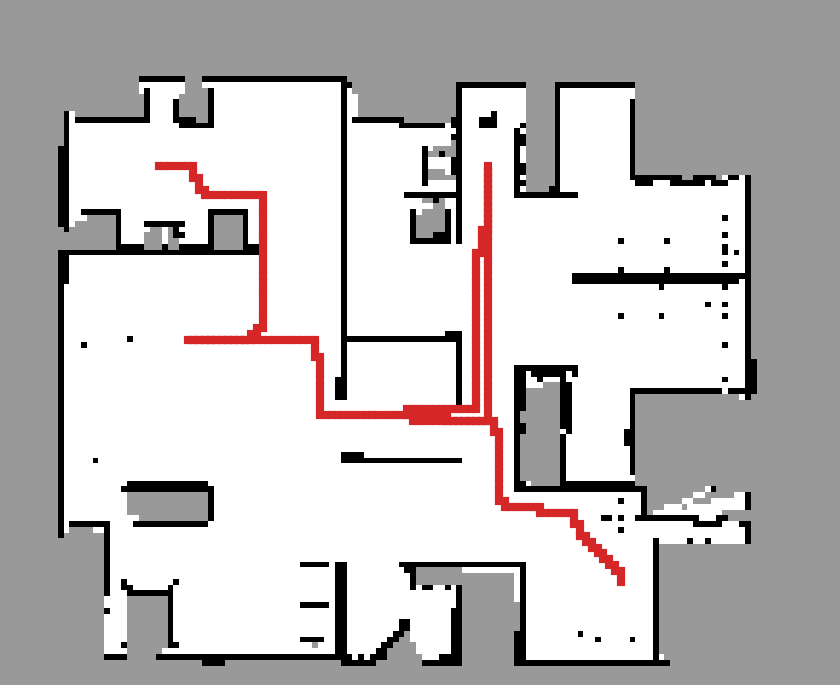
(c) HPP-II

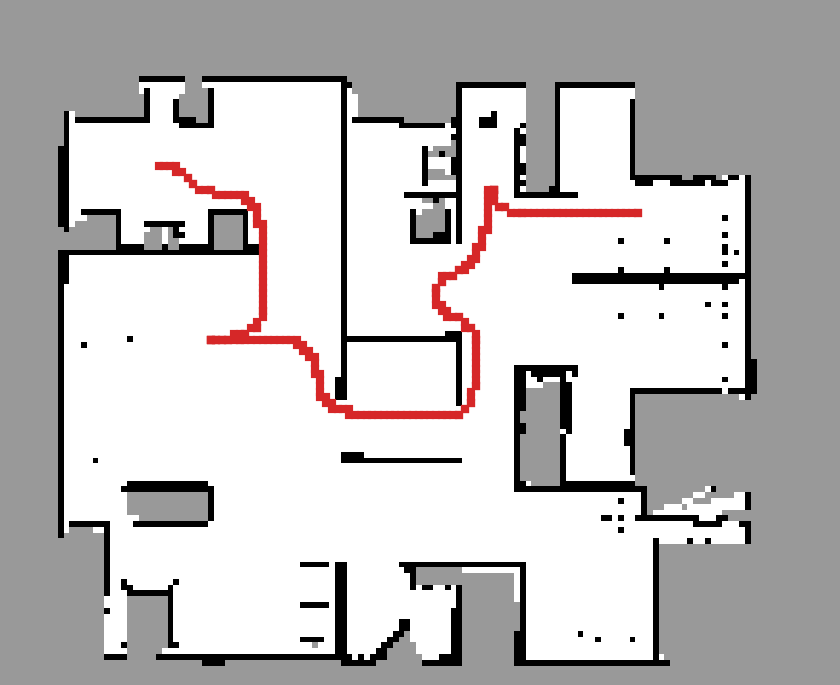
(d) SpCoTMHP

Figure 4: Example of path planning in the advanced task. The instruction: “Go to the bedroom via the lavatory.” (Experiment I).

TABLE II: Evaluation results of the path planning tasks (Experiment I).

			Basic task			Advanced task
Methods	Hierarchy	CaI	SPL$\uparrow$	N-SPL$\uparrow$	Time$\downarrow$	SPL$\uparrow$	W-SPL$\uparrow$	N-SPL$\uparrow$	WN-SPL$\uparrow$	Time$\downarrow$
A⋆	-	-	0.570	0.463	$9.47\times 10^{0}$	0.312	0.449	0.233	0.034	$9.44\times 10^{0}$
SpCoNavi (Viterbi)	-	✓	0.976	0.965	$2.68\times 10^{3}$	—	—	—	—	—
SpCoNavi (A⋆ approx.)	-	✓	0.404	0.388	$5.42\times 10^{1}$	0.266	0.308	0.252	0.013	$5.53\times 10^{1}$
HPP-I (path cost)	✓	-	0.723	0.605	$7.56\times 10^{0}$	0.917	0.248	0.773	0.191	$7.53\times 10^{0}$
HPP-II (path distance)	✓	-	0.714	0.571	$7.96\times 10^{0}$	0.902	0.250	0.729	0.183	$8.03\times 10^{0}$
SpCoTMHP	✓	✓	0.861	0.812	$\mathbf{4.79\times 10^{0}}$	0.922	0.906	0.794	0.781	$\mathbf{3.89\times 10^{-1}}$

Result: Table II shows the evaluation results for the basic and advanced planning tasks. Figure 4 shows the example of the estimated path. Overall, SpCoTMHP outperformed the comparison methods and significantly reduced the computation time. The basic task also demonstrated that the proposed method solves the problem of stopping the path before reaching the objective, which occurs in SpCoSNavi (A^⋆ approx.). The N-SPL of the baseline methods was lower than that of the proposed method because there were cases where the goal was chosen to be a bedroom far from the initial position. This demonstrated the effectiveness of the proposed method based on probabilistic inference (i.e., CaI).

The advanced task confirmed that the proposed method could estimate the path via the waypoint (Fig. 4(d)). Although SpCoTMHP has the disadvantage of estimating slightly redundant paths, the reduced computation time and improved planning performance make it a more practical approach than conventional methods. Consequently, the proposed method achieves better path planning by considering all the initial, waypoint, and goal positions.

VI Experiment II: Real environment

We demonstrate that the formation of spatial concepts, including the topological relations of places, can be realized in a real environment. Additionally, we confirm that the proposed method could plan a path based on the learned topometric semantic map.

VI-A Spatial concept-based topometric semantic mapping

Condition: The experimental environment was identical to that of the open dataset albert-b-laser-vision, which was obtained from the robotics dataset repository (Radish) [29]. The utterance was 70 sentences, such as “This is a dining room.” The hyperparameters for learning were set as follows: $\alpha=0.5$, $\gamma=0.05$, $\beta=0.1$, $\chi=1.0$, $\omega=0.5$, $m_{0}=[0,0]^{\rm T}$, $\kappa_{0}=0.001$, $V_{0}={\rm diag}(2,2)$, and $\nu_{0}=3$. The other settings were the same as in Experiment I.

Normalized mutual information (NMI) and adjusted Rand index (ARI), the most widely used metrics in clustering tasks for unsupervised learning, were used as the evaluation metrics for learning the spatial concept. NMI is obtained by normalizing the mutual information between the clustering result and the correct label in the 0.0–1.0 range. ARI is 1.0 when the clustering result matches the correct label and 0.0 when it is random.

Result: Figures 5 (a–d) show an example of learning the spatial concept. Table III shows the results of evaluating the average values of ten trials of spatial concept learning. SpCoTMHP achieved a higher learning performance than SpCoSLAM. In addition, the proposed method with reverse replay had the highest performance. For example, Fig. 5 (c) caused overlapping distributions in the upper right and skipped connections to neighboring distributions, whereas (d) mitigated these problems. As a result, it can be said that using place transitions during learning and vice versa is effective for learning spatial concepts.

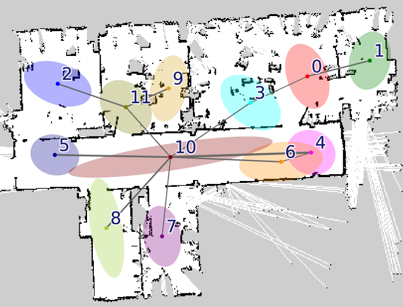
(a) Ideal semantic map

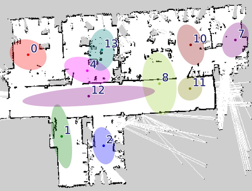
(b) SpCoSLAM

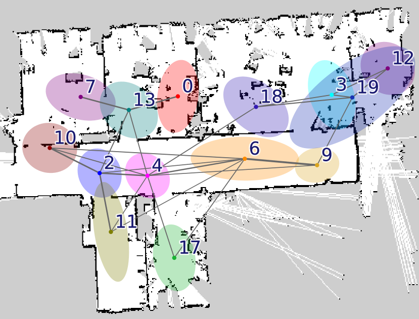
(c) SpCoTMHP

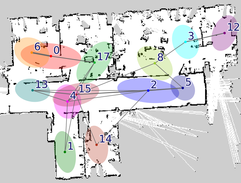
(d) SpCoTMHP (with reverse replay)

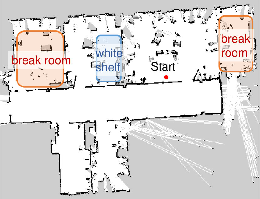
(e) Situation

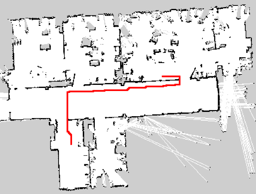
(f) SpCoNavi (A^⋆ approx.)

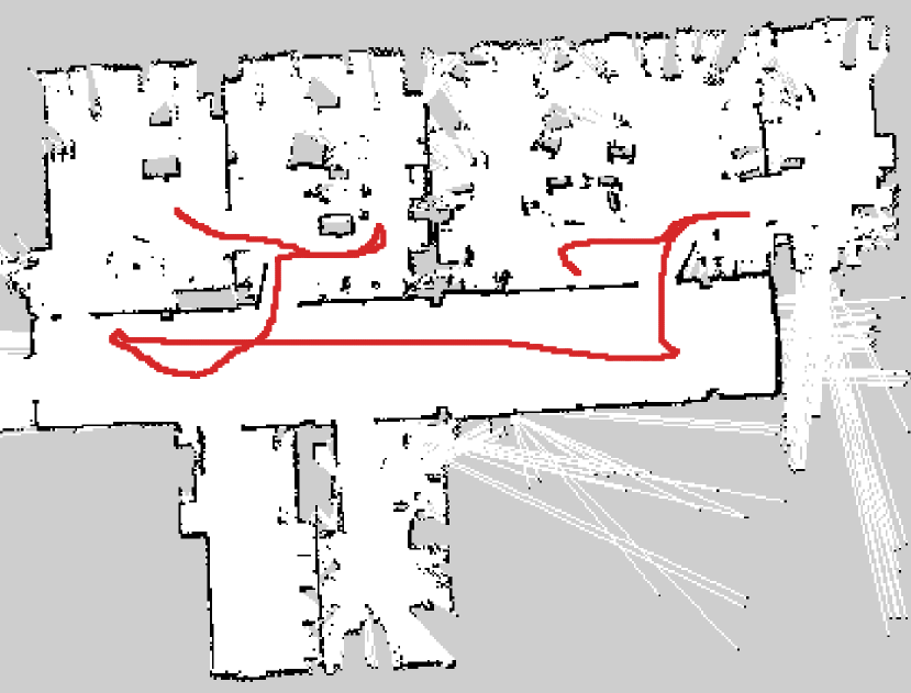
(g) SpCoTMHP

(h) SpCoTMHP (with reverse replay)

Figure 5: Top (a–d): Result of the spatial concept learning. Bottom (e–h): Result of path planning. The speech instruction is “Go to the break room via the white shelf.” The break room was taught in two rooms: the upper right and the upper left. The white shelf is in the second room from the left on the upper side. (Experiment II).

TABLE III: Performance of learning (Experiment II).

	NMI		ARI
Methods	$C_{e}$	$i_{e}$	$C_{e}$	$i_{e}$
SpCoSLAM	0.767	0.803	0.539	0.578
SpCoTMHP	0.779	0.858	0.540	0.656
SpCoTMHP (with reverse replay)	0.786	0.862	0.562	0.658

VI-B Path planning from speech instructions

The speech instruction was “Go to the break room via the white shelf.” The other settings were the same as in Experiment I. Figures 5 (e–h) show the results for path planning using the spatial concept. While SpCoSLAM could not reach the waypoint and goal, SpCoTMHP could estimate the path to reach the goal via the waypoint. The learning with reverse replay in (c) shortened the additional route that would result from the bias of the transition between places during learning in (b). The results show that the proposed method can accurately perform hierarchical path planning, although the learning results are imperfect, as shown in Table III.

VII Conclusions

We achieved topometric semantic mapping based on multimodal observations and hierarchical path planning through waypoint-guided instructions. Experimental results demonstrated improved performance in spatial concept learning and path planning, both in simulated and real-world environments. Additionally, the approximate inference achieved high computational efficiency, countering the model’s complexity.

The experiment assumed one waypoint; however, the proposed method will theoretically handle multiple waypoints. While the computation complexity increases with the topological planning horizon $E$, scalability will be sufficiently ensured when users only require a few waypoints. In this paper, we trained our model using the procedure described in Sec. IV-B. Simultaneous and online learning for the entire model is also possible with particle filters [18].

Future work will include utilizing foundation models and transferring knowledge of spatial adjacencies across multiple environments. Our method is computationally efficient, making it applicable to online path planning such as model predictive control. Additionally, the proposed model has the potential to enable visual navigation and linguistic path explanations through cross-modal inference.

References

- [1] I. Kostavelis and A. Gasteratos, “Semantic mapping for mobile robotics tasks: A survey,” Robotics and Autonomous Systems, vol. 66, pp. 86–103, 2015.
- [2] S. Garg, N. Sünderhauf, F. Dayoub, D. Morrison, A. Cosgun, G. Carneiro, Q. Wu, T.-J. Chin, I. Reid, S. Gould, P. Corke, and M. Milford, “Semantics for Robotic Mapping, Perception and Interaction: A Survey,” Foundations and Trends® in Robotics, vol. 8, no. 1â2, pp. 1–224, 2020.
- [3] G. Grisetti, C. Stachniss, and W. Burgard, “Improved Techniques for Grid Mapping with Rao-Blackwellized Particle Filters,” IEEE Transactions on Robotics, vol. 23, pp. 34–46, 2007.
- [4] S. Levine, “Reinforcement Learning and Control as Probabilistic Inference: Tutorial and Review,” arXiv, 2018.
- [5] K. Zheng, A. Pronobis, and R. P. N. Rao, “Learning Graph-Structured Sum-Product Networks for Probabilistic Semantic Maps,” in AAAI, 2018.
- [6] I. Kostavelis, K. Charalampous, A. Gasteratos, and J. K. Tsotsos, “Robot navigation via spatial and temporal coherent semantic maps,” Engineering Applications of Artificial Intelligence, vol. 48, pp. 173–187, 2016.
- [7] C. Gomez, M. Fehr, A. Millane, A. C. Hernandez, J. Nieto, R. Barber, and R. Siegwart, “Hybrid Topological and 3D Dense Mapping through Autonomous Exploration for Large Indoor Environments,” in IEEE ICRA, 2020, pp. 9673–9679.
- [8] A. Rosinol, A. Violette, M. Abate, N. Hughes, Y. Chang, J. Shi, A. Gupta, and L. Carlone, “Kimera: From SLAM to spatial perception with 3D dynamic scene graphs,” The International Journal of Robotics Research, vol. 40, pp. 1510–1546, 2021.
- [9] M. Hiller, C. Qiu, F. Particke, C. Hofmann, and J. Thielecke, “Learning Topometric Semantic Maps from Occupancy Grids,” in IEEE/RSJ IROS, 2019, pp. 4190–4197.
- [10] Y. C. N. Sousa and H. F. Bassani, “Topological semantic mapping by consolidation of deep visual features,” IEEE Robotics and Automation Letters, vol. 7, no. 2, pp. 4110–4117, 2022.
- [11] R. C. Holte and M. B. Perez, “Hierarchical A*,” in AAAI, 1996, pp. 530–535.
- [12] G. J. Stein, C. Bradley, V. Preston, and N. Roy, “Enabling Topological Planning with Monocular Vision,” in IEEE ICRA, 2020, pp. 1667–1673.
- [13] R. C. Luo and M. Chiou, “Hierarchical Semantic Mapping using Convolutional Neural Networks for Intelligent Service Robotics,” IEEE Access, vol. 6, pp. 61 287–61 294, 2018.
- [14] T. D. Kulkarni, K. R. Narasimhan, A. Saeedi, and J. B. Tenenbaum, “Hierarchical deep reinforcement learning: Integrating temporal abstraction and intrinsic motivation,” in NeurIPS, 2016, pp. 3682–3690.
- [15] R. Haarnoja, K. Hartikainen, P. Abbeel, and S. Levine, “Latent space policies for hierarchical reinforcement learning,” in ICML, vol. 4, 2018, pp. 2965–2975.
- [16] P. Anderson, Q. Wu, D. Teney, J. Bruce, M. Johnson, N. Sünderhauf, I. Reid, S. Gould, and A. van den Hengel, “Vision-and-language navigation: Interpreting visually-grounded navigation instructions in real environments,” in IEEE CVPR, 2018, pp. 3674–3683.
- [17] K. Chen, J. K. Chen, J. Chuang, M. Vázquez, and S. Savarese, “Topological Planning with Transformers for Vision-and-Language Navigation,” in IEEE CVPR, 2021, pp. 11 271–11 281.
- [18] A. Taniguchi, Y. Hagiwara, T. Taniguchi, and T. Inamura, “Online Spatial Concept and Lexical Acquisition with Simultaneous Localization and Mapping,” in IEEE/RSJ IROS, 2017, pp. 811–818.
- [19] M. J. Johnson and A. S. Willsky, “Bayesian Nonparametric Hidden Semi-Markov Models,” Journal of Machine Learning Research, vol. 14, pp. 673–701, 2013.
- [20] A. Taniguchi, Y. Hagiwara, T. Taniguchi, and T. Inamura, “Spatial Concept-Based Navigation with Human Speech Instructions via Probabilistic Inference on Bayesian Generative Model,” Advanced Robotics, vol. 34, no. 19, pp. 1213–1228, sep 2020.
- [21] A. Viterbi, “Error bounds for convolutional codes and an asymptotically optimum decoding algorithm,” IEEE transactions on Information Theory, vol. 13, no. 2, pp. 260–269, 1967.
- [22] K. P. Murphy, Machine learning: a probabilistic perspective. Cambridge, MA: MIT Press, 2012.
- [23] D. Gildea and T. Hofmann, “Topic-based Language Models Using EM,” in EUROSPEECH, 1999.
- [24] D. J. Foster and M. A. Wilson, “Reverse replay of behavioural sequences in hippocampal place cells during the awake state,” Nature, vol. 440, no. 7084, pp. 680–683, 2006.
- [25] A. Kinose and T. Taniguchi, “Integration of imitation learning using GAIL and reinforcement learning using task-achievement rewards via probabilistic graphical model,” Advanced Robotics, pp. 1–13, 2020.
- [26] T. Inamura and Y. Mizuchi, “SIGVerse: A Cloud-Based VR Platform for Research on Multimodal Human-Robot Interaction,” Frontiers in Robotics and AI, vol. 8, p. 158, 2021.
- [27] S. Niijima, R. Umeyama, Y. Sasaki, and H. Mizoguchi, “City-Scale Grid-Topological Hybrid Maps for Autonomous Mobile Robot Navigation in Urban Area,” in IEEE/RSJ IROS, 2020.
- [28] P. Anderson, A. Chang, D. S. Chaplot, A. Dosovitskiy, S. Gupta, V. Koltun, J. Kosecka, J. Malik, R. Mottaghi, M. Savva, and A. R. Zamir, “On Evaluation of Embodied Navigation Agents,” arXiv, 2018.
- [29] C. Stachniss, “The Robotics Data Set Repository (Radish),” 2003. [Online]. Available: https://dspace.mit.edu/handle/1721.1/62291