Hybrid Quantum-Classical Boson Sampling Algorithm for Molecular Vibrationally Resolved Electronic Spectroscopy with Duschinsky Rotation and Anharmonicity

Abstract

Using a photonic quantum computer for boson sampling has been demonstrated a tremendous advantage over classical supercomputers. It is highly desirable to develop boson sampling algorithms for realistic scientific problems. In this work, we propose a hybrid quantum-classical sampling (HQCS) algorithm to calculate the optical spectrum for complex molecules considering anharmonicity and Duschinsky rotation (DR) effects. The classical sum-over-state method for this problem has a computational complexity that exponentially increases with system size. In the HQCS algorithm, an intermediate harmonic potential energy surface (PES) is created, bridging the initial and final PESs. The magnitude and sign ($-1$ or $+1$) of the overlap between the initial state and the intermediate state are estimated by quantum boson sampling and by classical algorithms respectively, achieving an exponential speed-up. Additionally, the overlap between the intermediate state and the final state is efficiently evaluated by classical algorithms. The feasibility of HQCS is demonstrated in calculations of the emission spectrum of a Morse model as well as pyridine molecule by comparison with the nearly exact time-dependent density matrix renormalization group solutions. A near-term quantum advantage for realistic molecular spectroscopy simulation is proposed.

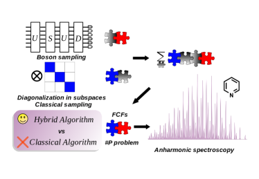
(a)

Figure 1: TOC graphic

I Introduction

In the early 1980s, Feynman proposed quantum computation as a natural solution for many-body problems hard for classical computers Feynman1982Simulating . Since then, many quantum algorithms have been devised to solve classically hard problems. However, the presently known methods such as Shor’s algorithm Shor1994algorithms for factorization and quantum phase estimation (QPE)Abrams1999Quantum for the eigenvalue problems require an error-tolerant quantum computer which is not available in the near future. Variational quantum algorithms  Peruzzo2014variational , hybridizing classical and quantum computation, is regarded as a practical choice for quantum computation applications with the current noisy intermediate-scale quantum (NISQ) device. On the other hand, quantum advantage has been reported through quantum sampling algorithms such as random circuit sampling arute2019quantum , boson sampling Aaronson2011the ; wang2019boson and its variants Gaussian boson sampling (GBS) hamilton2017gaussian ; Zhong2020quantum ; Zhong2021Phase . Recently, quantum computer "Jiu Zhang 2.0" performed GBS on a $\sim 10^{43}$ large Hilbert space which was shown to be $\sim 10^{24}$ faster than a brute-force simulation on the state-of-the-art classical computers  Zhong2020quantum ; Zhong2021Phase . Currently, it is valuable to develop algorithms that profit from the quantum advantage of the quantum sampling algorithms and devices to solve practical problems.

In this work, we focus on the computation of molecular vibrationally resolved electronic spectrum taking both Duschinsky rotation (DR) and anharmonicity into account. DR refers to the mode-mixing between the normal modes of the initial and final states in complex molecular systems. A number of experimental  Shen2018quantum ; Clements2018approximating ; Wang2020Efficient and theoretical  Huh2015boson ; Jnane2021Analog works have focused on the simulation of molecular spectrum with DR effect under harmonic approximation using the boson sampling algorithms. It should be noted that such problem has been solved exactly and analytically on classical computers by Peng et al. by the thermal vibration correlation function (TVCF) method back in 2007  Peng2007Excited ; niu2008promoting . Hence, there is no point to demonstrate quantum advantages for such a problem. Besides the DR effect, the anharmonic effect on molecular spectrum has also been found to be very important in general for complex molecules, especially, for flexible molecules  Petrenko2017General ; liang2006electronic ; heimel2005breakdown . To calculate the spectrum with both anharmonicity and DR is indeed a hard problem for classical algorithms because there is no analytical solution and the numerical approaches have an exponential scaling with the number of modes. Therefore, it is necessary to develop quantum algorithms for such a problem, while no near-term solutions have been proposed yet. The previously suggested boson sampling algorithms can only simulate Franck-Condon factors (FCFs) between harmonic states, so they are not suitable for anharmonic spectrum. Vibrational relaxation of anharmonic Hamiltonian using vibrational pertubation theory to consider influence from all third derivatives and the semi-diagonal quartic derivatives had been simulated using nonlinear optics in analogue quantum simulation (sparrow2018simulating, ), but this method cannot deal with more general anharmonic potential energy surface (PES). QPE based solutions have been reported to calculate eigenstates on anharmonic potential McArdle2019Digital and anharmonic spectrum Sawaya2019Quantum , but unable to realize with NISQ device.

In this work, we propose a hybrid quantum-classical sampling (HQCS) algorithm to calculate the molecular vibrationally resolved electronic spectrum including both the anharmonic effect and the DR effect. We first present an analysis of the computational complexity for this classically hard problem. Second, we will describe the HQCS algorithm in detail, which includes three sub-components. The effectiveness of this HQCS algorithm is then demonstrated by calculating the emission spectrum of a two-mode model as well as a pyridine molecule using a simulator for photonic quantum computer. We believe that the real quantum device can accelerate the calculations in the near term.

II Results

II.1 Analysis of the complexity of computing molecular vibrationally resolved electronic spectrum

The molecular vibrationally resolved electronic spectrum is commonly calculated under the Born-Oppenheimer approximation Lin2002Ultrafast , in which two adiabatic electronic states are considered, denoted with subscript “i/f” for the initial/final electronic state (Symbols without subscript refer to a general state). With mass-weighted rectilinear coordinates, the Hamiltonian can be expressed as

$$\hat{H}_{0}=\sum_{n=1}^{N}-\frac{1}{2}\frac{\partial^{2}}{\partial q_{n}^{2}}+\left[\begin{matrix}V_{\mathrm{f}}(\mathbf{q})&0\\ 0&V_{\mathrm{i}}(\mathbf{q})\\ \end{matrix}\right],$$ (1)

where $N$ is the total number of modes. $\mathbf{q}\equiv\{q_{1},q_{2},\cdots,q_{N}\}$ indicates that the PES $V$ is a multi-dimensional function. For semi-rigid molecules, it is preferred to express PES in the normal coordinates, because the mode coupling in this coordinate system is minimized. The two sets of normal coordinates of the initial and final PESs are related by the DR matrix $\mathbf{S}$ and the normal-mode-projected displacement $\Delta\mathbf{q}$.

$$\mathbf{q}_{\mathrm{f}} =\mathbf{S}\mathbf{q}_{\mathrm{i}}+\Delta\mathbf{q}_{\mathrm{f}}$$ (2)

The lowest order approximation to PES is the harmonic approximation,

$$V=\sum_{n}\frac{1}{2}\omega_{n}^{2}q_{n}^{2}+V_{\textrm{eq}}$$ (3)

Beyond that, the PES can be hierarchically expanded as 1-mode terms, 2-mode terms, 3-mode terms, etc., which is known as the $n$-mode representation ($n$-MR) li2001high ; bowman2003multimode . In this work, we only consider 1-MR PES, in which the intra-mode anharmonicity is included and the modes are still independent of each other.

$$V=\sum_{n}V_{n}(q_{n})+V_{\textrm{eq}}$$ (4)

With Fermi’s golden rule and Condon’s approximation, the optical transition rate at zero temperature can be expressed as

$$\sigma_{\textrm{abs/emi}}(E)=|\mu_{\textrm{if}}|^{2}\sum_{v_{\mathrm{f}}}|\langle\phi_{\mathrm{i}}^{\mathbf{0}}(\mathbf{q}_{\mathrm{i}})|\phi_{\mathrm{f}}^{\mathbf{v}_{\mathrm{f}}}(\mathbf{q}_{\mathrm{f}})\rangle|^{2}\delta(E_{\mathrm{f},{\mathbf{v}_{\mathrm{f}}}}+E-E_{\mathrm{i},\mathbf{0}})$$ (5)

$|\phi_{\mathrm{i/f}}^{\mathbf{v}_{\mathrm{i/f}}}\rangle$ is the initial/final vibrational state with configuration $\mathbf{v}_{\mathrm{i/f}}$. $\mu_{\textrm{if}}$ is the transition dipole moment. At zero temperature, the harmonic approximation is reasonable for $V_{\textrm{i}}$, but is inappropriate for $V_{\textrm{f}}$, because the optical transition starts from the equilibrium geometry of the initial state, which however could be far from the equilibrium geometry of the final state if the electron-vibration coupling is largewang2009anharmonic . Therefore, in this work, $V_{\mathrm{i}}$ is described by a harmonic PES (Eq. (3)) and $V_{\mathrm{f}}$ is described by a 1-MR PES (Eq. (4)).

Unlike the harmonic spectrum with analytical solution, no accurate and efficient classical algorithm for the anharmonic spectrum has been proposed yet to calculate Eq. (5). The computational cost of the sum-over-state algorithm will exponentially increase with the system size for the following two reasons. First, the multi-dimensional integration of FCFs $|\langle\phi_{\mathrm{i}}(\mathbf{q}_{\mathrm{i}})|\phi_{\mathrm{f}}(\mathbf{q}_{\mathrm{f}})\rangle|^{2}$ with DR has been recognized as a $\#P$ problemHuh2015boson with exponential computational scaling on classical computers. Second, the summation over $\mathbf{v}_{\mathrm{f}}$ is also an exponentially hard problem for classical computers, because the dimension of the Hilbert space increases exponentially with the system size (if $d$ vibrational states are considered in each mode, the number of $\mathbf{v}_{\textrm{f}}$ is $d^{N}$). To overcome these two exponentially hard problems, we propose a hybrid quantum-classical sampling algorithm. The details are described in the next section.

II.2 hybrid quantum-classical sampling algorithm

The key to the HQCS algorithm is to build an intermediate harmonic PES, $V_{\mathrm{m}}=\sum_{n}\frac{1}{2}\omega_{\mathrm{m},n}^{2}q_{\mathrm{m},n}^{2}$ and insert its complete eigenbasis set into Eq. (5).

$$\sigma_{\mathrm{abs/emi}}(E)=|\mu_{\textrm{if}}|^{2}\sum_{\mathbf{v}_{\mathrm{f}}}|\sum_{\mathbf{v}_{\mathrm{m}}}\langle\phi_{\mathrm{i}}^{\mathbf{0}}(\mathbf{q}_{\mathrm{i}})|\phi_{\mathrm{m}}^{\mathbf{v}_{\mathrm{m}}}(\mathbf{q}_{\mathrm{m}})\rangle\langle\phi_{\mathrm{m}}^{\mathbf{v}_{\mathrm{m}}}(\mathbf{q}_{\mathrm{m}})|\phi_{\mathrm{f}}^{\mathbf{v}_{\mathrm{f}}}(\mathbf{q}_{\mathrm{f}})\rangle|^{2}$$ (6)

$$\delta(E_{\mathrm{f},{\mathbf{v}_{\mathrm{f}}}}+E-E_{\mathrm{i},\mathbf{0}})$$

It seems that the evaluation of Eq. (6) is even more complicated compared to Eq. (5). But, with a smart choice of the parameters of the intermediate PES and taking advantage of both quantum and classical sampling algorithms, Eq.(6) can be efficiently calculated. The two requirements of $V_{\mathrm{m}}$ is that i) $\omega_{\mathrm{m},n}=\mathrm{max}(\omega_{\mathrm{f},n},\omega_{\mathrm{i},n})$; ii) $\mathbf{q}_{\mathrm{m}}=\mathbf{q}_{\mathrm{f}}$. With this intermediate PES, there are three steps to evaluate Eq.(6), which are

1. estimation of $\langle\phi_{\mathrm{i}}^{\mathbf{0}}(\mathbf{q}_{\mathrm{i}})|\phi_{\mathrm{m}}^{\mathbf{v}_{\mathrm{m}}}(\mathbf{q}_{\mathrm{m}})\rangle$;

2. estimation of $\langle\phi_{\mathrm{m}}^{\mathbf{v}_{\mathrm{m}}}(\mathbf{q}_{\mathrm{m}})|\phi_{\mathrm{f}}^{\mathbf{v}_{\mathrm{f}}}(\mathbf{q}_{\mathrm{f}})\rangle$;

3. summation over $\mathbf{v}_{\mathrm{m}}$ and $\mathbf{v}_{\mathrm{f}}$.

The schematic flowchart is shown in FIG. 2. The first requirement is key to approximating the sign of $\langle\phi_{\mathrm{i}}^{\mathbf{0}}(\mathbf{q}_{\mathrm{i}})|\phi_{\mathrm{m}}^{\mathbf{v}_{\mathrm{m}}}(\mathbf{q}_{\mathrm{m}})\rangle$. The second requirement is to make the estimation of $\langle\phi_{\mathrm{m}}^{\mathbf{v}_{\mathrm{m}}}(\mathbf{q}_{\mathrm{m}})|\phi_{\mathrm{f}}^{\mathbf{v}_{\mathrm{f}}}(\mathbf{q}_{\mathrm{f}})\rangle$ much easier. In the following, we replace $\mathbf{q}_{\mathrm{m}}$ with $\mathbf{q}_{\mathrm{f}}$ for simplicity. The Dirac delta function in Eq. (6) is broadened with Gaussian function $\delta(E_{\mathrm{f},{\mathbf{v}_{\mathrm{f}}}}+E-E_{\mathrm{i},\mathbf{0}})\to e^{-\frac{(E-E_{\mathrm{i},\mathbf{0}}+E_{\mathrm{f},{\mathbf{v}_{\mathrm{f}}}})^{2}}{2\sigma^{2}}}$.

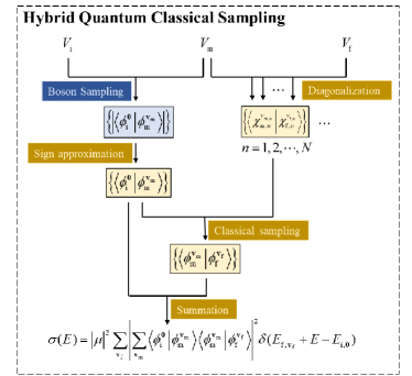
Figure 2: A schematic flowchart of Hybrid Quantum-Classical Sampling algorithm calculating the optical spectroscopy for transition from harmonic PES $V_{\mathrm{i}}$ to anharmonic and Duschinsky-rotated PES $V_{\mathrm{f}}$ by introducing a harmonic and Duschinsky-rotated PES $V_{\mathrm{m}}$ . Blue steps are performed on the quantum device, while yellow steps are performed on the classical computer.

II.2.1 estimation of $\langle\phi_{\mathrm{i}}^{\mathbf{0}}(\mathbf{q}_{\mathrm{i}})|\phi_{\mathrm{m}}^{\mathbf{v}_{\mathrm{m}}}(\mathbf{q}_{\mathrm{f}})\rangle$

The calculation of the overlap $\langle\phi_{\mathrm{i}}^{\mathbf{0}}(\mathbf{q}_{\mathrm{i}})|\phi_{\mathrm{m}}^{\mathbf{v}_{\mathrm{m}}}(\mathbf{q}_{\mathrm{f}})\rangle$ between two harmonic wavefunctions with DR is a classically hard problem as we discussed in Section  II.1. Here, we propose to calculate the norm and the sign ($-1$ or $+1$) separately. The former can be obtained through boson sampling on a quantum device. The latter can be approximated by a classical algorithm.

The Doktorov unitary operator $\mathbf{\hat{U}}_{\mathrm{Dok}}$ can connect two harmonic wavefunctions with rotation, distortion, and displacement  doktorov1975dynamical ; doktorov1977dynamical . The expression of $\mathbf{\hat{U}}_{\mathrm{Dok}}$ can be found in the literatureQuesada2019franck ; barnett2002methods (See the Supplementary Information for more details). Hence, the FCFs can be expressed as

$$|\langle\phi_{\mathrm{i}}^{\mathbf{0}}(\mathbf{q}_{\mathrm{i}})|\phi_{\mathrm{m}}^{\mathbf{v}_{\mathrm{m}}}(\mathbf{q}_{\mathrm{f}})\rangle|^{2}= |\langle\varphi_{\mathrm{i}}^{\mathbf{0}}(\mathbf{R}_{\mathrm{i}})|\varphi_{\mathrm{m}}^{\mathbf{v}_{\mathrm{m}}}(\mathbf{R}_{\mathrm{f}})\rangle|^{2}$$

$$= |\langle\varphi_{\mathrm{i}}^{\mathbf{0}}(\mathbf{R}_{\mathrm{f}})|\mathbf{\hat{U}}_{\mathrm{Dok}}|\varphi_{\mathrm{m}}^{\mathbf{v}_{\mathrm{m}}}(\mathbf{R}_{\mathrm{f}})\rangle|^{2}.$$ (7)

where $\mathbf{R}$ is the dimensionless normal coordinates as $\mathbf{R}=\mathbf{\omega}^{\frac{1}{2}}\mathbf{q}$ and $\phi(\mathbf{q})=\varphi(\mathbf{R})$. The right-hand side of Eq. (7) is the same as the expression describing the sampling probability $P$ of one specific output harmonic state $|\phi_{\mathrm{m}}^{\mathbf{v}_{\mathrm{m}}}\rangle$ for an input harmonic state $|\phi_{\mathrm{i}}^{\mathbf{0}}\rangle$ passing through an interferometer accounted by unitary transformation $\mathbf{\hat{U}}_{\mathrm{Dok}}$ during the boson sampling process. The sampling probability has been confirmed as a $\#P$ problem hard on classical computers Aaronson2011the but can be efficiently simulated with the boson sampling algorithm using a quantum device. Because of the equivalence, the boson sampling algorithm Huh2015boson ; Jnane2021Analog has been proposed to simulate FCFs between two harmonic states, in which the sampling probability $P_{\mathbf{v}_{\mathrm{i}}\rightarrow\mathbf{v}_{\mathrm{m}}}$ corresponds to the magnitude of FCFs. Thus, the norm can be obtained, that is,

$$|\langle\phi_{\mathrm{i}}^{\mathbf{0}}(\mathbf{q}_{\mathrm{i}})|\phi_{\mathrm{m}}^{\mathbf{v}_{\mathrm{m}}}(\mathbf{q}_{\mathrm{f}})\rangle|=\sqrt{P_{\mathbf{0}\rightarrow\mathbf{v}_{\mathrm{m}}}}.$$ (8)

The next step is to approximate the sign. For a one-dimensional problem, previous works lin2007Symmetric ; lin2010theoretical have derived an analytic expression of the overlap between two one-mode harmonic wavefunctions $|\chi\rangle$. The detailed expression at zero temperature is given in the method section. When $\omega_{\mathrm{m},n}=\mathrm{max}(\omega_{\mathrm{f},n},\omega_{\mathrm{i},n})\geq\omega_{\mathrm{i},n}$, the sign of the overlap can be obtained through Eq. (9).

$$\mathrm{sgn}(\langle\chi_{\mathrm{i},n}^{0}(q_{\mathrm{f},n})|\chi_{\mathrm{m},n}^{v_{\mathrm{m},n}}(q_{\mathrm{i},n})\rangle)=(\mathrm{sgn}(\Delta q_{\mathrm{f},n}))^{v_{\mathrm{m},n}}$$ (9)

Thus, if without DR,

$$\mathrm{sgn}(\langle\phi_{\mathrm{i}}^{\mathbf{0}}(\mathbf{q}_{\mathrm{i}})|\phi_{\mathrm{m}}^{\mathbf{v}_{\mathrm{m}}}(\mathbf{q}_{\mathrm{f}})\rangle)=\prod_{n}^{N}(\mathrm{sgn}(\Delta q_{\mathrm{f},n}))^{v_{\mathrm{m},n}}$$ (10)

With DR, the factorized formula above is not exact anymore. However, considering that the amplitude of the initial ground vibrational state is positive and nodeless, if DR only occurs between modes with the same frequency, DR will not change the sign of the overlap. Fortunately, in molecular systems, DR commonly occurs within groups of modes having close frequencies. Therefore, it can be speculated that DR could hardly flip the sign of the overlap and thus Eq. (10) is still a good approximation. To verify the assumption, we calculate the sign of a two-mode and a four-mode model numerically in the Supplementary Information. The results showed that the assumption is quite reliable. However, it should be noted that this approximation to the sign of the overlap is only reliable for the ground vibrational state as initial state, which limits our algorithm to the zero temperature case currently.

II.2.2 estimation of $\langle\phi_{\mathrm{m}}^{\mathbf{v}_{\mathrm{m}}}(\mathbf{q}_{\mathrm{f}})|\phi_{\mathrm{f}}^{\mathbf{v}_{\mathrm{f}}}(\mathbf{q}_{\mathrm{f}})\rangle$

As the coordinates of $\phi_{\mathrm{m}}^{\mathbf{v}_{\mathrm{m}}}$ and $\phi_{\mathrm{f}}^{\mathbf{v}_{\mathrm{f}}}$ are the same and the modes are assumed to be independent,

$$\langle\phi_{\mathrm{m}}^{\mathbf{v}_{\mathrm{m}}}(\mathbf{q}_{\textrm{f}})|\phi_{\textrm{f}}^{\mathbf{v}_{\mathrm{f}}}(\mathbf{q}_{\textrm{f}})\rangle=\prod_{n}\langle\chi_{\mathrm{m}}^{v_{{\mathrm{m}},n}}(q_{\textrm{f},n})|\chi_{\mathrm{f}}^{v_{\mathrm{f},n}}(q_{\textrm{f},n})\rangle,$$ (11)

where $\langle\chi_{\mathrm{m}}^{v_{{\mathrm{m}},n}}(q_{\textrm{f},n})|\chi_{\mathrm{f}}^{v_{\mathrm{f},n}}(q_{\textrm{f},n})\rangle$ is an one-dimensional problem and thus is quite easy to calculate on classical computers. Using the harmonic states $\{|\chi_{\mathrm{m}}^{v_{{\mathrm{m}},n}}\rangle\}$ with a cutoff on $v_{\mathrm{m},n}$ as the primitive basis set, we can obtain the corresponding discrete variable representation (DVR) basis set light1985generalized and the transformation matrix between the primitive harmonic basis and the DVR basis. The matrix elements of $\hat{H}_{\mathrm{f},n}=-\frac{1}{2}\frac{\partial^{2}}{\partial q_{\mathrm{f},n}^{2}}+V_{\mathrm{f},n}(q_{\mathrm{f},n})$ can be first expanded in DVR basis and then transformed to the primitive harmonic basis. Through exact diagonalizaiton of this Hamiltonian, the eigenstates $\{|\chi_{\mathrm{f}}^{v_{\mathrm{f},n}}\rangle\}$ are obtained, so are their overlaps with the primitive basis. For an $N$-mode system with $d$ basis functions for each mode, the cost of the current sub-step has a linear scaling with the system size, i.e., $O(Nd^{3})$. Finally, it should be noted that although the number of the overlap matrix elements $\langle\phi_{\mathrm{m}}^{\mathbf{v}_{\mathrm{m}}}(\mathbf{q}_{\mathrm{f}})|\phi_{\mathrm{f}}^{\mathbf{v}_{\mathrm{f}}}(\mathbf{q}_{\mathrm{f}})\rangle$ is exponentially large, only the dominant elements sampled out in the next section actually need to be calculated.

II.2.3 summation over $\mathbf{v}_{\mathrm{m}}$ and $\mathbf{v}_{\mathrm{f}}$

The last step is to make the summation over $\mathbf{v}_{\mathrm{m}}$ and $\mathbf{v}_{\mathrm{f}}$ in Eq. (6). Although the total number of $\mathbf{v}_{\mathrm{m}}$ and $\mathbf{v}_{\mathrm{f}}$ both grow exponentially with the system size, in realistic systems only a small portion of the vibrational states with large FCFs determines the vibrational structure in electronic spectrum. Because the boson sampling will naturally screen out $\mathbf{v}_{\mathrm{m}}$ with dominant $|\langle\phi_{\mathrm{i}}^{\mathbf{0}}|\phi_{\mathrm{m}}^{\mathbf{v}_{\mathrm{m}}}\rangle|^{2}$, the summation over $\mathbf{v}_{\mathrm{m}}$ in Eq. (6) will be classically efficient Dierksen2005efficient ; Santoro2007effective . Given a specific $\mathbf{v}_{\mathrm{m}}$, the dominant $\mathbf{v}_{\mathrm{f}}$ can also be obtained according to the weight $|\langle\chi_{\mathrm{m},n}^{v_{\mathrm{m},n}}|\chi_{\mathrm{f},n}^{v_{\mathrm{f},n}}\rangle|^{2}$ by a classical sampling (CS) algorithm. A schematic flowchart of CS is shown in FIG. 3. It consists of $\Omega_{\mathrm{CS}}$ sampling loops, among each of which a weighted random sampling is first performed for the intermediate vibrational state configuration $\mathbf{v}_{\mathrm{m}}=(\cdots,v_{\mathrm{m},n},\cdots)$ with the weight $|\langle\phi_{\mathrm{i}}^{\mathbf{0}}|\phi_{\mathrm{m}}^{\mathbf{v}_{\mathrm{m}}}\rangle|^{2}$ collected from boson sampling result. Then, given one $\mathbf{v}_{\mathrm{m}}$, another weighted random sampling is carried out for $v_{\mathrm{f},n}$ with the weight $|\langle\chi_{\mathrm{m},n}^{v_{\mathrm{m},n}}|\chi_{\mathrm{f},n}^{v_{\mathrm{f},n}}\rangle|^{2}$ calculated in Section II.2.2. After each loop, the newly appeared $\mathbf{v}_{\mathrm{f}}=(\cdots,v_{\mathrm{f},n},\cdots)$ will be collected. The eventual summations over $\mathbf{v}_{\mathrm{f}}$ is done only for those sampled out. The upper bound of the number of summations is $O(M_{\mathrm{m}}M_{\mathrm{f}})$, where $M_{\mathrm{m/f}}$ are the number of intermediate/final state configurations sampled by boson sampling/CS. From CS, we can also obtain a set of $\{(\mathbf{v}_{\mathrm{m}},\mathbf{v}_{\mathrm{f}})\}$ pairs. The size of this set $M_{\mathrm{pair}}$ should be smaller than $M_{\mathrm{m}}M_{\mathrm{f}}$. Hence, for higher efficiency, we can just sum over this paired set $\{(\mathbf{v}_{\mathrm{m}},\mathbf{v}_{\mathrm{f}})\}$, giving cost $O(M_{\mathrm{pair}})$.

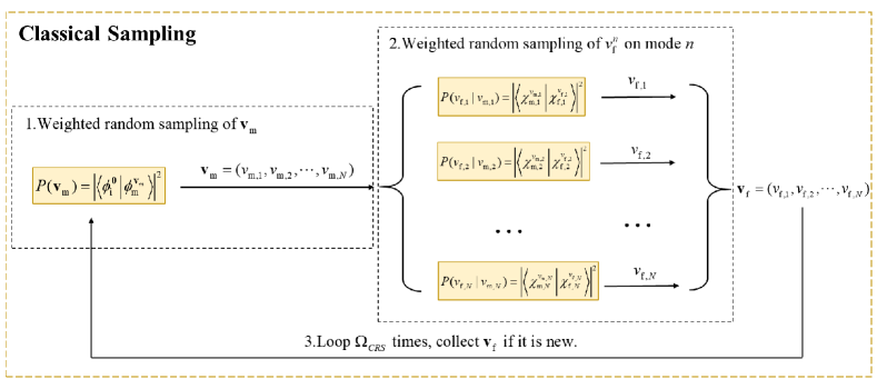
Figure 3: A schematic flowchart of the classical sampling step used in HQCS.

For molecules with complex spectrum, we need to sample some small probability events to achieve high resolution. For such a purpose, a tunable bias $k$ can be added on the weight for CS such that $P(v_{\mathrm{f},n}|v_{\mathrm{m},n})=\frac{|\langle\chi_{\mathrm{m},n}^{v_{\mathrm{m},n}}|\chi_{\mathrm{f},n}^{v_{\mathrm{f},n}}\rangle|^{2/k}}{\sum_{v_{\mathrm{f},n}}{|\langle\chi_{\mathrm{m},n}^{v_{\mathrm{m},n}}|\chi_{\mathrm{f},n}^{v_{\mathrm{f},n}}\rangle|^{2/k}}}$ to enhance the probability for sampling less probable events.

II.3 Results

In order to validate the HQCS algorithm, we use the python package “strawberry fields”Killoran2019strawberryfields and “Walrus” Gupt2019the to simulate the quantum boson sampling on classical computers. The results are compared with reference spectrum calculated by the nearly-exact time-dependent density matrix renormalization group (TD-DMRG) method with the package Renormalizer Renormalizer developed by our group. We calculate the emission spectrum of a two-mode model with initial excited state PES $V_{\mathrm{i}}$ as harmonic potential and the final ground state PES $V_{\mathrm{f}}$ as Morse potential. The intermediate PES $V_{\mathrm{m}}$ is obtained by performing harmonic expansion at equilibrium point on the Morse potential $V_{\mathrm{f}}$. This model has been used previously to investigate the anharmonic effect on the internal conversion processwang2021evaluating ; Ianconescu2011Semiclassical . Harmonic frequency and Morse parameters on the different between modes here and more details and parameters can be seen in the Supplementary Information. The DR matrix $\mathbf{S}$ between the PESs is parameterized by an angle $\theta$.

$$\mathbf{S}=\left[\begin{matrix}\mathrm{cos}\theta&-\mathrm{sin}\theta\\ \mathrm{sin}\theta&\mathrm{cos}\theta\\ \end{matrix}\right]$$ (12)

The spectrum with different $\theta$ are shown in FIG. 4. No matter $\theta$ is 0, $\pi/4$, or $\pi/2$, the HQCS algorithm reproduces the results of TD-DMRG quite well.

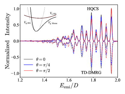
Figure 4: The emission spectrum of the two-mode Morse model. The reference spectrum produced by TD-DMRG are shown on the bottom panel (dashed lines). On the top (solid lines) are results produced by HQCS. Different $\theta$ values are used to manipulate the Duschinsky rotation effects. The intensity is normalized by the highest peak of the spectrum. Inset is the schematic PES along one mode of the two-mode Morse model. The initial excited state PES $V_{\mathrm{e},\mathrm{HA}}$ is harmonic (top thick line) and the final ground state PES $V_{\mathrm{g},\mathrm{Morse}}$is Morse (bottom thick line). Performing harmonic approximation on $V_{\mathrm{g},\mathrm{Morse}}$ at equilibrium point, we obtain $V_{\mathrm{g},\mathrm{HA}}$ (bottom thin line), which is used as the intermediate PES.

Furthermore, we move to a real molecular system: the $S_{1}$ to $S_{0}$ emission spectrum of pyridine. Previous studies have used the perturbation method to handle the third-order force constantswang2009anharmonic of $S_{0}$ PES to investigate the anharmonic effect on the emission spectrum. In our calculations, the electronic structure of pyridine and normal mode analysis are calculated at the B3LYP/6-31g(d) level with Gaussian 16 package g16 . Following that, the DR matrix $\mathbf{S}$, the displacement $\Delta\mathbf{q}$ are calculated by the program MOMAPniu2018molecular developed by our group. For the anharmonicity, 1-MR $S_{0}$ PES fitted with polynomial functions up to 12th order is constructed by the adaptive density-guided approach implemented in MidasCpp  midascpp developed by Christiansen et al. sparta2009adaptive . From a total of 27 normal modes, we select 7 important modes involving large displacements or DR effect for the HQCS simulation. For the rest 20 modes, only the difference in their zero-point energies of $S_{0}$ and $S_{1}$ PESs are considered, which shifts the spectrum. Detailed information of electronic structure calculation on pyridine and the way to select important modes are given in Supplementary Information. There, the reduced 7-mode model is demonstrated to be sufficient for the emission spectrum of pyridine. Limited by the capability of the quantum simulator, we allow a maximum of 5 quanta on one mode for boson sampling and sampling $\Omega_{\mathrm{BS}}=10^{5}$ times in total. The HQCS simulated emission spectrum are shown in FIG. 5 in comparison with TD-DMRG (The experimental fluorescence spectrum Yamazaki1977Observation is also shown). It shows that HQCS can well reproduce the features in the spectrum. The deviations at the weak-intensity peak originate from the limited sampling times and the cutoff on quanta. These deviations are expected to reduce with a real boson sampling device, which can simulate sufficiently large quanta and sampling times.

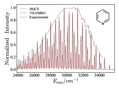
Figure 5: The $S_{1}$ to $S_{0}$ emission spectrum of pyridine calculated with HQCS (red solid line) and reference result obtained by TD-DMRG (black dashed line). The anharmonic $S_{0}$ is approximated using 1-MR PES. The final states configurations $\mathbf{v}_{\mathrm{f}}$ are sampled by CS with $10^{4}$ loop times, altogether $M_{\mathrm{f}}=936$ different configurations of $\mathbf{v}_{\mathrm{f}}$ are sampled out based on $M_{\mathrm{m}}=1806$ configurations of $\mathbf{v}_{\mathrm{m}}$ sampled by boson sampling. The experimental results (’Experimental’, black dotted curves) is also showed. spectrum are normalized with their highest peak. The theoretical (HQCS & TD-DMRG) results have been blue-shifted by 1350 $\textrm{cm}^{-1}$ for better correspondence.

Table 1: Comparison of the number of configurations sampled with different $\Omega_{\mathrm{CS}}$.

$\Omega_{\mathrm{CS}}$	Number of sampled configuration $v_{\mathrm{f}}$	$\sum_{\mathbf{v}_{\mathrm{f}}}|\sum_{\mathbf{v}_{\mathrm{m}}}\langle\phi_{\mathrm{i}}^{\mathbf{0}}|\phi_{\mathrm{m}}^{\mathbf{v}_{\mathrm{m}}}\rangle\langle\phi_{\mathrm{m}}^{\mathbf{v}_{\mathrm{m}}}|\phi_{\mathrm{f}}^{\mathbf{v}_{\mathrm{f}}}\rangle|^{2}$
$10^{1}$	10	0.023
$10^{2}$	78	0.362
$10^{3}$	359	0.824
$10^{4}$	936	0.969
$10^{5}$	1797	0.996

The deviation of $\sum_{\mathbf{v}_{\mathrm{f}}}|\sum_{\mathbf{v}_{\mathrm{m}}}\langle\phi_{\mathrm{i}}^{\mathbf{0}}|\phi_{\mathrm{m}}^{\mathbf{v}_{\mathrm{m}}}\rangle\langle\phi_{\mathrm{m}}^{\mathbf{v}_{\mathrm{m}}}|\phi_{\mathrm{f}}^{\mathbf{v}_{\mathrm{f}}}\rangle|^{2}$ from 1 can be used as a measure of whether the classical sampling process is converged or not. Table. 1 shows the results with different $\Omega_{\mathrm{CS}}$. The results indicate that the summation over 936 final configurations $\mathbf{v}_{\mathrm{f}}$ from CS after $10^{4}$ loops and with 1806 intermediate configurations $\mathbf{v}_{\mathrm{m}}$ from the boson sampling can already give a quantitatively correct spectrum (the deviation is less than 5%). It should be noted that the whole size of the final configuration space is $10^{7}$ (10 quanta for each of the 7 modes). Namely, the HQCS algorithm can vastly reduce the computational cost for the summation.

III Discussion

To perform the HQCS algorithm on an actual photonic quantum device, more error sources including photon loss, noise, and distinguishabilityClements2018approximating should be considered. The HQCS algorithm described in this work can be further improved for higher efficiency in specific cases. For example, considering that the real experimental devices have limitations on the maximum number of quanta (basis cutoff) simulated on one optical modeWang2020Efficient , the intermediate PES $V_{\mathrm{m}}(\mathbf{q}_{\mathrm{m}})$ in HQCS should be fine-tuned to reduce the basis size needed on each optical mode to simulate the important configurations with large FCFs. One prescription is to decease the displacement between $\mathbf{q}_{\mathrm{i}}$ and $\mathbf{q}_{\mathrm{m}}$ because larger displacement often leads to larger overlap between $|\phi_{\mathrm{i}}^{\mathbf{0}}\rangle$ and high level $|\phi_{\mathrm{m}}^{\mathbf{v}_{\mathrm{m}}}\rangle$ .

In conclusion, we have proposed a hybrid quantum-classical sampling algorithm, combining the boson sampling on quantum devices and the classical sampling on classical computers, for simulating molecular vibrationally resolved electronic spectroscopy including both Duschinsky rotation effect and anharmonic effect. Although the current algorithm is only for the zero temperature case and independent modes, the simplified problem is still classically hard. The effectiveness of the HQCS algorithm is demonstrated in a two-mode Morse potential model and pyridine molecule by comparing with the nearly exact TD-DMRG method. Moreover, as we have intentionally designed the HQCS algorithm to contain only one step of boson sampling that have already been realized in many platforms Clements2018approximating ; Shen2018quantum ; Wang2020Efficient and other three steps on robust classical computers, we suggest HQCS is a practical near-term quantum simulation scheme to achieve quantum advantage for molecular spectroscopy and boost relating photophysical and photochemical research.

IV Methods

IV.1 Time correlation function formalism of spectrum

spectrum from TD-DMRG for benchmark are obtained from the time correlation function (TCF) formalism. Here we will give a brief introduction. Detailed derivations can be seen from our former worksRen2018Time ; Li2020Numerical . Performing Fourier transformation of Delta function in Eq.(5) and then removing the completeness relation $\mathbf{I}=\sum_{\mathbf{v}_{\mathrm{f}}}|\phi_{\mathrm{f}}^{\mathbf{v}_{\mathrm{f}}}(\mathbf{q}_{\mathrm{f}})\rangle\langle\phi_{\mathrm{f}}^{\mathbf{v}_{\mathrm{f}}}(\mathbf{q}_{\mathrm{f}})|$, we can obtain the TCF formalism as Eq.(13). By TD-DMRG, the TCF $C(t)$ is first calculated within a finite time period and then is Fourier transformed to obtain the spectrum.

$$\sigma_{\textrm{abs/emi}}(E) =|\mu_{\textrm{if}}|^{2}\int_{-\infty}^{\infty}dt\,e^{-iEt}C(t)$$

$$C(t) =e^{iE_{\mathrm{i},\mathbf{0}}t}\langle\phi_{\mathrm{i}}^{\mathbf{0}}(\mathbf{q}_{\mathrm{i}})|e^{-i\hat{H}_{\textrm{f}}t}|\phi_{\mathrm{i}}^{\mathbf{0}}(\mathbf{q}_{\mathrm{i}})\rangle$$ (13)

IV.2 Parameters for computation

IV.2.1 The spectrum of the 2-mode Morse model

For HQCS, the quanta cutoff is 15 for each mode to perform boson sampling, which are operated $10^{4}$ times. Simple harmonic basis with frequency $\omega_{\mathrm{m},n}$ and size as 60 are used for each mode $n$ as primitive basis set in the exact diagonalization. Only 15 lowest eigenstates of each mode are used in the summation step. The whole Hilbert space is very small and thus CS is not needed here. For the reference spectrum produced by TD-DMRG, simple harmonic oscillator basis with frequency $\omega_{\mathrm{f},n}$ and size as 60 are used for each mode $n$ as primitive basis set. Bond dimension $M_{S}$ for matrix product state (MPS) is 10 for the initial state optimization and 4 for time evolution. 400 steps are propagated with time-step size $\Delta t=8\,\mathrm{a.u.}$ to calculate the TCF. The spectrum is broadened by a Gaussian function with $\sigma=10^{-3}\,\mathrm{a.u.}$. Corresponding DVR basis are used to expand the Morse form potential operator and then transformed to the primitive basis for both methods.

IV.2.2 The spectrum of pyridine

For HQCS, the quanta cutoff is 5 for each mode to perform boson sampling because of the heavy computational cost of the classical simulation of the boson sampling algorithm. $10^{5}$ times of boson sampling operation are simulated. Simple harmonic oscillator basis with frequency $\omega_{\mathrm{m},n}$ and size as 60 on each mode $n$ are used in the exact diagonalization and only the lowest 10 eigenstates on each mode are used in CS and then the summation step. For the reference spectrum produced by TD-DMRG, simple harmonic oscillator basis with frequency as $\omega_{\mathrm{f},n}$ and size as 60 are used for each mode $n$. Bond dimension $M_{S}$ for MPS is 40 for the initial state optimization and 10 for time evolution. 1200 steps are propagated with time-step size $\Delta t=32\,\mathrm{a.u.}$ to calculate TCF. The spectrum is broadened by a Gaussian function with $\sigma=10^{-4}\,\mathrm{a.u.}$. DVR basis is not used here because pyridine 1-MR PES in this work is described by polynomial functions so the matrix elements of potential operator on simple harmonic oscillator basis used is analytical.

IV.3 Analytical expression of the overlap between one-dimensional harmonic states

$$\langle\chi_{\mathrm{i}}^{0}|\chi_{\mathrm{m}}^{v_{\mathrm{m}}}\rangle=\Gamma(\Delta q_{\mathrm{f}})^{v_{\mathrm{m}}}\times(\sum_{l}C_{l})$$ (14)

$$C_{l}= \frac{(-1)^{v_{\mathrm{m}}-l}+1}{2}(\Delta q_{\mathrm{f}})^{-(v_{\mathrm{m}}-l)}\beta_{\mathrm{m}}^{l/2}$$ (15)

$$\frac{2^{l}}{l!}(\frac{\beta_{\mathrm{i}}}{\beta_{\mathrm{i}}+\beta_{\mathrm{m}}})^{l}(\frac{\beta_{\mathrm{m}}-\beta_{\mathrm{i}}}{\beta_{\mathrm{i}}+\beta_{\mathrm{m}}})^{\frac{v_{\mathrm{m}}-l}{2}}\frac{1}{(\frac{v_{\mathrm{m}}-l}{2})!}$$

$$\Gamma= (\frac{v_{\mathrm{m}}!}{2^{v_{\mathrm{m}}}}\times\frac{2\sqrt{\beta_{\mathrm{i}}\beta_{\mathrm{m}}}}{\beta_{\mathrm{i}}+\beta_{\mathrm{m}}})^{\frac{1}{2}}\mathrm{exp}(-\frac{\beta_{\mathrm{i}}\beta_{\mathrm{m}}(\Delta q_{\mathrm{f}})^{2}}{2(\beta_{\mathrm{i}}+\beta_{\mathrm{m}})})$$

where $\beta_{\mathrm{i}}=\omega_{\mathrm{i}}/\hbar$, $l$ are non-negative integers meeting the condition $l\leq v_{\mathrm{m}}$. As $\Gamma$-function is always non-negative and $C_{l}$ is non-negative when $\omega_{\mathrm{m},n}$ $\geq$ $\omega_{\mathrm{i},n}$, the sign of the overlap only depends on the sign of the displacement $\Delta q_{\mathrm{f}}$ and the quanta $v_{\mathrm{m}}$ of the intermediate state.

V references

VI Acknowledgment

This work is supported by the National Natural Science Foundation of China Grant Nos. 21788102 and by the Ministry of Science and Technology of China through the National Key R&D Plan Grant No. 2017YFA0204501

VII Author contributions

Z.S. supervised the study. Y.W. performed the numerical calculations, analyzed the data, and wrote the manuscript with the help of J.R and W.L

VIII Competing interests

The authors declare no competing interests.

IX Materials & Correspondence

Correspondence and requests for materials should be addressed to Z.S.

References

- (1) Feynman, R. P. Simulating physics with computers, International Journal of Theoretical Physics 21, 467–488 (1982).
- (2) Shor, P. Algorithms for quantum computation: discrete logarithms and factoring. In Proceedings 35th Annual Symposium on Foundations of Computer Science, 124–134, (1994).
- (3) Abrams, D. S. and Lloyd, S. Quantum algorithm providing exponential speed increase for finding eigenvalues and eigenvectors, Phys. Rev. Lett. 83, 5162–5165 (1999).
- (4) Peruzzo, A. et.al. A variational eigenvalue solver on a photonic quantum processor, Nature Communications 5, 4213 (2014).
- (5) Arute, F. et.al. Quantum supremacy using a programmable superconducting processor, Nature 574, 505–510 (2019).
- (6) Aaronson, S. and Arkhipov, A. The computational complexity of linear optics. In Proceedings of the Forty-Third Annual ACM Symposium on Theory of Computing, STOC ’11, 333–342 (Association for Computing Machinery, New York, NY, USA, 2011).
- (7) Wang, H. et.al. Boson sampling with 20 input photons and a 60-mode interferometer in a -dimensional hilbert space, Phys. Rev. Lett. 123, 250503 (2019).
- (8) Hamilton, C. S., Kruse, R., Sansoni, L., Barkhofen, S., Silberhorn, C., and Jex, I. Gaussian boson sampling, Phys. Rev. Lett. 119, 170501 (2017).
- (9) Zhong, H.-S. et.al. Quantum computational advantage using photons, Science 370, 1460–1463 (2020).
- (10) Zhong, H.-S. et.al. Phase-programmable gaussian boson sampling using stimulated squeezed light, Phys. Rev. Lett. 127, 180502 (2021).
- (11) Shen, Y., Lu, Y., Zhang, K., Zhang, J., Zhang, S., Huh, J., and Kim, K. Quantum optical emulation of molecular vibronic spectroscopy using a trapped-ion device, Chem. Sci. 9, 836–840 (2018).
- (12) Clements, W. R. et.al. Approximating vibronic spectroscopy with imperfect quantum optics, J. Phys. B: At. Mol. Opt. Phys 51, 245503 (2018).
- (13) Wang, C. S. et.al. Efficient multiphoton sampling of molecular vibronic spectra on a superconducting bosonic processor, Phys. Rev. X 10, 021060 (2020).
- (14) Huh, J., Guerreschi, G. G., Peropadre, B., McClean, J. R., and Aspuru-Guzik, A. Boson sampling for molecular vibronic spectra, Nature Photonics 9, 615–620 (2015).
- (15) Jnane, H., Sawaya, N. P. D., Peropadre, B., Aspuru-Guzik, A., Garcia-Patron, R., and Huh, J. Analog quantum simulation of non-condon effects in molecular spectroscopy, ACS Photonics 8, 2007–2016 (2021).
- (16) Peng, Q., Yi, Y., Shuai, Z., and Shao, J. Excited state radiationless decay process with duschinsky rotation effect: formalism and implementation, J. Chem. Phys. 126, 114302 (2007).
- (17) Niu, Y., Peng, Q., and Shuai, Z. Promoting-mode free formalism for excited state radiationless decay process with duschinsky rotation effect, Science in China Series B: Chemistry 51, 1153–1158 (2008).
- (18) Petrenko, T. and Rauhut, G. A general approach for calculating strongly anharmonic vibronic spectra with a high density of states: photoelectron spectrum of difluoromethane, J. Chem. Theory Comput. 13, 5515–5527 (2017).
- (19) Liang, W., Zhao, Y., Sun, J., Song, J., Hu, S., and Yang, J. Electronic excitation of polyfluorenes: A theoretical study, J. Phys. Chem. B 110, 9908–9915 (2006).
- (20) Heimel, G. et.al. Breakdown of the mirror image symmetry in the optical absorption/emission spectra of oligo(para-phenylene)s, J. Chem. Phys. 122, 054501 (2005).
- (21) Sparrow, C. et.al. Simulating the vibrational quantum dynamics of molecules using photonics, Nature 557, 660–667 (2018).
- (22) McArdle, S., Mayorov, A., Shan, X., Benjamin, S., and Yuan, X. Digital quantum simulation of molecular vibrations, Chem. Sci. 10, 5725–5735 (2019).
- (23) Sawaya, N. P. D. and Huh, J. Quantum algorithm for calculating molecular vibronic spectra, J. Phys. Chem. Lett. 10, 3586–3591 (2019).
- (24) Lin, S. et.al. Ultrafast dynamics and spectroscopy of bacterial photosynthetic reaction centers, Adv. Chem. Phys. 121, 1–88 (2002).
- (25) Li, G., Rosenthal, C., and Rabitz, H. High dimensional model representations, J. Phys. Chem. A 105, 7765–7777 (2001).
- (26) Bowman, J. M., Carter, S., and Huang, X. Multimode: a code to calculate rovibrational energies of polyatomic molecules, Int. Rev. Phys. Chem. 22, 533–549 (2003).
- (27) Wang, H., Zhu, C., Yu, J.-G., and Lin, S. H. Anharmonic franck-condon simulation of the absorption and fluorescence spectra for the low-lying s1 and s2 excited states of pyridine, J. Phys. Chem. A 113, 14407–14414 (2009).
- (28) Doktorov, E., Malkin, I., and Man’Ko, V. Dynamical symmetry of vibronic transitions in polyatomic molecules and the franck-condon principle, J. Mol. Spectrosc. 56, 1–20 (1975).
- (29) Doktorov, E., Malkin, I., and Man’Ko, V. Dynamical symmetry of vibronic transitions in polyatomic molecules and the franck-condon principle, J. Mol. Spectrosc. 64, 302–326 (1977).
- (30) Quesada, N. Franck-condon factors by counting perfect matchings of graphs with loops, J. Chem. Phys. 150, 164113 (2019).
- (31) Barnett, S. and Radmore, P. M. Methods in theoretical quantum optics, volume 15. Oxford University Press, (2002).
- (32) Lin, C.-K., Chang, H.-C., and Lin, S. H. Symmetric double-well potential model and its application to vibronic spectra: Studies of inversion modes of ammonia and nitrogen-vacancy defect centers in diamond, J. Phys. Chem. A 111, 9347–9354 (2007).
- (33) Lin, C.-K., Li, M.-C., Yamaki, M., Hayashi, M., and Lin, S. H. A theoretical study on the spectroscopy and the radiative and non-radiative relaxation rate constants of the vibronic transitions of formaldehyde, Phys. Chem. Chem. Phys. 12, 11432–11444 (2010).
- (34) Light, J., Hamilton, I., and Lill, J. Generalized discrete variable approximation in quantum mechanics, J. Chem. Phys. 82, 1400–1409 (1985).
- (35) Dierksen, M. and Grimme, S. An efficient approach for the calculation of franck-condon integrals of large molecules, J. Chem. Phys. 122, 244101 (2005).
- (36) Santoro, F., Improta, R., Lami, A., Bloino, J., and Barone, V. Effective method to compute franck-condon integrals for optical spectra of large molecules in solution, J. Chem. Phys. 126, 084509 (2007).
- (37) Killoran, N., Izaac, J., Quesada, N., Bergholm, V., Amy, M., and Weedbrook, C. Strawberry Fields: A Software Platform for Photonic Quantum Computing, Quantum 3, 129 (2019).
- (38) Gupt, B., Izaac, J., and Quesada, N. The walrus: a library for the calculation of hafnians, hermite polynomials and gaussian boson sampling, J. Open. Source. Softw 4, 1705 (2019).
- (39) Renormalizer. https://github.com/shuaigroup/Renormalizer.
- (40) Wang, Y., Ren, J., and Shuai, Z. Evaluating the anharmonicity contributions to the molecular excited state internal conversion rates with finite temperature td-dmrg, J. Chem. Phys. 154, 214109 (2021).
- (41) Ianconescu, R. and Pollak, E. Semiclassical initial value representation study of internal conversion rates, J. Chem. Phys. 134, 234305 (2011).
- (42) Frisch, M. J. et.al. Gaussian˜16 Revision C.01. Gaussian Inc. Wallingford CT, 2016.
- (43) Niu, Y. et.al. Molecular materials property prediction package (momap) 1.0: a software package for predicting the luminescent properties and mobility of organic functional materials, Mol. Phys. 116, 1078–1090 (2018).
- (44) Christiansen, O. Midascpp. https://gitlab.com/midascpp/midascpp.
- (45) Sparta, M., Toffoli, D., and Christiansen, O. An adaptive density-guided approach for the generation of potential energy surfaces of polyatomic molecules, Theor. Chem. Acc. 123, 413–429 (2009).
- (46) Yamazaki, I. and Baba, H. Observation of fluorescence of pyridine in the vapor phase, J. Chem. Phys. 66, 5826–5827 (1977).
- (47) Ren, J., Shuai, Z., and Kin-Lic Chan, G. Time-dependent density matrix renormalization group algorithms for nearly exact absorption and fluorescence spectra of molecular aggregates at both zero and finite temperature, J. Chem. Theory Comput. 14, 5027–5039 (2018).
- (48) Li, W., Ren, J., and Shuai, Z. Numerical assessment for accuracy and gpu acceleration of td-dmrg time evolution schemes, J. Chem. Phys. 152, 024127 (2020).