Tree Energy Loss: Towards Sparsely Annotated Semantic Segmentation

Abstract

Sparsely annotated semantic segmentation (SASS) aims to train a segmentation network with coarse-grained (i.e., point-, scribble-, and block-wise) supervisions, where only a small proportion of pixels are labeled in each image. In this paper, we propose a novel tree energy loss for SASS by providing semantic guidance for unlabeled pixels. The tree energy loss represents images as minimum spanning trees to model both low-level and high-level pair-wise affinities. By sequentially applying these affinities to the network prediction, soft pseudo labels for unlabeled pixels are generated in a coarse-to-fine manner, achieving dynamic online self-training. The tree energy loss is effective and easy to be incorporated into existing frameworks by combining it with a traditional segmentation loss. Compared with previous SASS methods, our method requires no multi-stage training strategies, alternating optimization procedures, additional supervised data, or time-consuming post-processing while outperforming them in all SASS settings. Code is available at https://github.com/megvii-research/TreeEnergyLoss.

1 Introduction

Figure 1: Illustration of current SASS approaches. $\mathcal{S}$ and $\mathcal{E}$ denote the segmentation and auxiliary models, respectively. Our method leverages the minimum spanning trees (MSTs) to capture both low-level and high-level affinities to generate soft pseudo labels, performing online self-training.

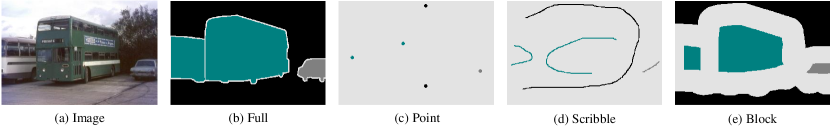
Figure 2: Different types of training annotations for semantic segmentation. The background class is annotated in black.

Semantic segmentation, aiming to assign each pixel a semantic label for given images, is one of the fundamental tasks in computer vision. Previous methods [4, 18, 26, 25, 36] tend to leverage large amounts of fully annotated labels like Fig. 2(b) to achieve satisfying performance. However, manually annotating such high-quality labels is labor-intensive. To reduce the annotation cost and preserve the segmentation performance, some recent works research on semantic segmentation with sparse annotations, such as point-wise [2] and scribble-wise ones [17]. As shown in Fig. 2(c-d), the point-wise annotation assigns each semantic object with a single-pixel label while the scribble-wise annotation draws at least a scribble label for the object.

As illustrated in Fig. 1(a-d), existing approaches are mainly based on auxiliary tasks, pseudo proposals, regularized losses, and consistency learning to solve SASS. However, there are some shortcomings in these approaches. The predictive error from the auxiliary task [34, 35, 15] may hinder the performance of semantic segmentation. The proposal generation [17, 42, 39] is time-consuming and usually calls for a multi-stage training strategy. The regularized losses [29, 30, 20, 21, 32] ignore the domain gap between the visual information and the high-level semantics, and the consistency learning [22, 24, 13, 3, 44, 45] fails to directly supervise the unlabeled pixels at the category level. In this paper, we aim to alleviate these shortcomings and introduce a simple yet effective solution.

In SASS, each image can be divided into labeled and unlabeled regions. The labeled region can be directly supervised by the ground truth, while how to learn from the unlabeled region is an open question. For the region of the same object, the labeled and unlabeled pixels share similar patterns on low-level color (RGB value of image) and high-level responses (features produced by CNN). Utilizing such similarity prior in SASS is intuitive. Inspired by the tree filter [1, 41], which can model the pair-wise similarity with its structure-preserving property, we leverage this property to generate soft pseudo labels for unlabeled regions and achieve online self-training.

Specifically, we introduce a novel tree energy loss (TEL) based on the low-level and the high-level similarities of image (see Fig. 1(e)). In TEL, two minimum spanning trees (MSTs) are built on the low-level color and the high-level semantic features, respectively. Each MST is obtained by sequentially eliminating connections between adjacent pixels with large dissimilarity, so less related pixels are separated and the essential relation among pixels is preserved. Then, two structure-aware affinity matrices obtained by accumulating the edge weights along the MSTs are multiplied with the network predictions in a cascading manner, producing soft pseudo labels. Finally, the generated pseudo labels are assigned to the unlabeled regions. Combining the TEL with a standard segmentation loss (e.g., cross-entropy loss), any segmentation network can learn extra knowledge from unlabeled regions via dynamic online self-training.

To comprehensively validate the effectiveness of TEL, we further enrich the SASS scenarios by introducing a block-wise annotation setting (see Fig. 2(e)), where the amount of annotations is located between the full and scribble settings. In this way, we can grade the SASS into three levels, i.e., point, scribble, and block. Experimental results show that TEL can significantly boost segmentation performance without introducing extra computational costs during inference. Equipped with recent segmentation networks, our method can achieve state-of-the-art performance under various annotated settings.

The main contributions are summarized as follow. We propose a novel tree energy loss (TEL) for SASS. TEL leverages minimum spanning trees to model the low-level and high-level structural relation among pixels. A cascaded filtering operation is further introduced to dynamically generate soft pseudo labels from network predictions in a coarse-to-fine way. TEL is clean and easy to be plugged into most existing segmentation networks. For comprehensive validation, we further introduce a block-annotated setting for SASS. Our method outperforms the state-of-the-arts under the point-, scribble- and block-annotated settings.

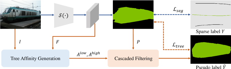
Figure 3: Flowchart of the proposed single-stage SASS method, which is realized by incorporating an auxiliary branch into the traditional segmentation model $\mathcal{S}(\cdot)$. During training, the predicted masks $P$ are split into the labeled and unlabeled parts, which are supervised by the segmentation loss $\mathcal{L}_{seg}$ and the tree energy loss $\mathcal{L}_{tree}$, respectively. To obtain pseudo labels for unlabeled pixels, the Tree Affinity Generation procedure (Eqs. 3-5) first utilizes the color information $I$ and semantic features $F$ to generate the low-level and high-level affinity matrices $A^{low},A^{high}$. Then the Cascaded Filtering operation (Eqs. 6-7) converts the network predictions $P$ into soft pseudo labels $\tilde{Y}$. During testing, the auxiliary branch is removed to avoid extra computational costs.

2 Related Works

Sparsely Annotated Semantic Segmentation: Sparsely annotated semantic segmentation aims to train the segmentation model with coarse-grained annotated data. Previous works mainly focus on the point-level and the scribble-level supervisions. What’s the Point [2] first presents the semantic segmentation task with point annotations. It combines the objectness prior, the image-level supervision, and point-level supervision into the loss function. PDML [24] proposes the point-based distance metric learning to model the intra- and inter-category relations across images. WeClick [19] utilizes temporal information of the video sequence and distills the semantic knowledge from a more complex model. Seminar [3] introduces seminar learning through EMA-based teacher models. To narrow the performance gap with fully annotated methods, an increasing number of scribble-annotated semantic segmentation methods have appeared. ScribbleSup [17] constructs a graphical model to alternatively propagate the scribble annotations and learn the model parameters. RAWKS [34] and BPG [35] adopt edge detectors to progressively refine the predictions for sharper semantic boundaries. A²GNN [42] blends the multi-level supervision and solves the segmentation problem with graph neural networks. PSI [39] utilizes multi-stage semantic features to progressively infer the predictions and pseudo labels. URSS [22] learns to reduce the uncertainty of the segmentation model by random walks, coupled with a self-supervised learning strategy. To capture the relation between labeled and unlabeled pixels, a variety of regularized losses [29, 30, 20, 21] are proposed. These methods use the low-level (i,e., spatial and color) information of images and train the model in two stages. In the first stage, the segmentation model is just trained with segmentation loss. Then a regularized loss is further adopted to fine-tune the model in the second stage.

Tree Filter: Modeling pair-wise relation is significant for many computer vision tasks. Regarding an image as an undirected planar graph, where nodes are all pixels and edges between adjacent nodes are weighted by the appearance dissimilarity, the minimum spanning tree (MST) can be constructed by removing edges according to substantial weights. Since the gradient between adjacent pixels can be viewed as the intensity of object boundaries, the nodes tend to interact with each other preferentially within the same object on the tree. Due to the structure-preserving property of MST, the traditional tree filters are applied in stereo matching [40, 41], salient object detection [33], image smoothing [1], denoising [27], and abstraction [14]. Recently, LTF [26] presents a learnable tree filter to capture the long-range dependencies for semantic segmentation. LTF-V2 [25] combines the learnable tree filter and the Markov Random Field [16] to further improve the performance.

3 Methodology

In this section, we first emphasize our motivation in Sec. 3.1. Then the overall architecture combining the traditional segmentation loss with the proposed tree energy loss (TEL) is introduced in Sec. 3.2. After that, we describe the details of TEL in Sec. 3.3. Finally, we discuss the main differences from previous related works in Sec. 3.4.

3.1 Motivation

The SASS task aims to train a dense prediction model with coarse-grained (i.e., point-, scribble- or block-wise) labels, where the annotations of most pixels are invisible during training. In SASS, the whole image can be separated into two parts: labeled set $\Omega_{L}$ and unlabeled set $\Omega_{U}$. For the labeled set $\Omega_{L}$, one can simply use the corresponding ground truth for training. As for the $\Omega_{U}$, it tends to be ignored in the traditional semantic segmentation framework, resulting in performance degradation. This paper aims to present a simple yet effective solution for SASS. Since pixels belonging to the same object share similar patterns at different feature levels, we leverage these similarities to provide the additional supervision for unlabeled pixels in $\Omega_{U}$. Inspired by tree filter [1, 41, 26], we model such pair-wise similarity based on its structure-preserving property. The pair-wise similarity together with the network prediction is used to generate soft pseudo labels for unlabeled pixels. Cooperated with the supervised learning in $\Omega_{L}$, an online self-training framework is constructed, achieving the progressive improvement of both network predictions and pseudo labels during training.

3.2 Overall Architecture

Fig. 3 illustrates the overall architecture of our method, which is composed of a segmentation branch for labeled pixels and an auxiliary branch for unlabeled pixels. The segmentation branch assigns the sparsely annotated label $Y$ to the labeled pixels. For the auxiliary branch, the pair-wise affinity matrices $A^{low}$, $A^{high}$ are generated from the original image $I$ and the embedded features $F$. Then the affinity matrices $A^{low}$, $A^{high}$ are used to refine the network prediction $P$ and generate soft pseudo label $\tilde{Y}$. The soft labels generated are assigned to the unlabeled pixels. Therefore, the overall loss function includes a segmentation loss $\mathcal{L}_{seg}$ and a tree energy loss $\mathcal{L}_{tree}$,

$$\mathcal{L}=\mathcal{L}_{seg}+\lambda\mathcal{L}_{tree},$$ (1)

where $\lambda$ is a balance factor for two losses. By leveraging two losses jointly, complementary knowledge can be learned by the whole segmentation network. For the $\mathcal{L}_{seg}$, we follow previous works [29, 30, 20, 21, 19] and formulate it as a partial cross-entropy loss:

$$\mathcal{L}_{seg}=-\frac{1}{|\Omega_{L}|}\sum_{\forall{i}\in\Omega_{L}}Y_{i}\log(P_{i}),$$ (2)

where $P_{i}$ and $Y_{i}$ are the network prediction and the corresponding ground truth at the location $i$. As for the proposed $\mathcal{L}_{tree}$, it will be presented in the next section.

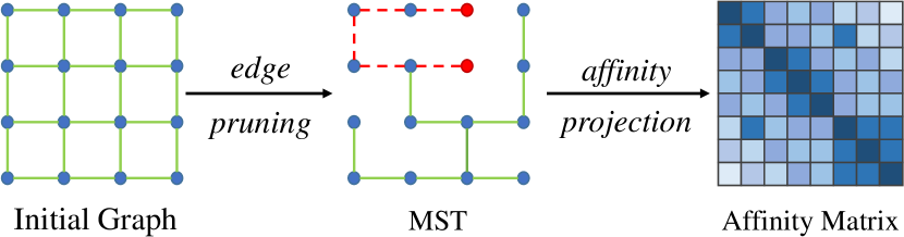
Figure 4: The process of Tree Affinity Generation. An initial graph is first built on the given low-level color or high-level semantic features, then the MST is obtained by the edge pruning algorithm [9]. On the MST, the distance between two vertices is calculated by the sum of edge weights along their hyper-edge. An example is illustrated in red dashed lines. Finally, the affinity projection is conducted to project the distance map into an affinity matrix.

3.3 Tree Energy Loss

Given the training images with sparse annotations, TEL learns to provide category guidance for unlabeled pixels. The TEL mainly includes the following three steps: (1) A tree affinity generation step to model the pair-wise relation. (2) A cascaded filtering step to generate pseudo labels. (3) A soft label assignment step to assign pseudo labels for unlabeled pixels. Here, we will introduce TEL in detail.

Tree Affinity Generation. An image can be represented as an undirected graph $G=(V,E)$, where the vertice set $V$ consists of all pixels and the edges between two adjacent vertices make up the edge set $E$. As shown in Fig. 4, we adopt the architecture of a 4-connected planar graph, where each pixel is adjacent to up to 4 neighboring ones. Let the vertice $i$ and vertice $j$ be adjacent on the graph, the low-level and high-level weight functions between them can be respectively defined as

$$\omega^{low}_{i,j}=\omega^{low}_{j,i}={|I(i)-I(j)|}^{2},$$ (3)

$$\omega^{high}_{i,j}=\omega^{high}_{j,i}={|F(i)-F(j)|}^{2},$$

where $I(i)\in\mathbb{R}^{3\times h\times w}$ and $F(i)\in\mathbb{R}^{256\times h\times w}$ are the RGB color and the semantic features of pixel $i$, respectively. $h$ and $w$ are the height and width of the downsampled input image. $F(i)$ is produced by a $1\times 1$ convolutional layer, from the features before the classification layer of the segmentation model. Once obtained the edge weights, a MST can be constructed by sequentially removing the edge with the largest weight from $E$ while ensuring the connectivity of the graph. We construct both the low-level and the high-level MSTs with the Bor$\mathring{u}$vka algorithm [9]. Based on the topology of MST, vertices within the same object share similar feature representations and tend to interact with each other preferentially.

Similar to [41, 26], the distance between two vertices of the MST can be calculated by the weight summation of their connected edges. And the distance of the shortest path between vertices, denoted as the hyper-edge $\mathbb{E}$, forms the distance map of the MST,

$$D^{*}_{i,j}=D^{*}_{j,i}=\sum_{(k,m)\in\mathbb{E}^{*}_{i,j}}\omega^{*}_{k,m},$$ (4)

where $i$, $j$, $k$ and $m$ are vertice indexes, $*\in\{low,high\}$. To capture the long-range relation among vertices, we project the distance maps to positive affinity matrices,

$$A^{low}=\exp\left(-D^{low}/{\sigma}\right),$$ (5)

$$A^{high}=\exp\left(-D^{high}\right),$$

where $\sigma$ is a preset constant value to modulate the color information. Given a training image, the low-level affinity $A^{low}$ is static while the high-level affinity $A^{high}$ is dynamic during training. They capture pair-wise relations at different feature levels. By utilizing them jointly, complementary knowledge can be learned.

Cascaded Filtering. Since the low-level affinity matrix $A^{low}$ contains object boundary information while the high-level affinity matrix $A^{high}$ maintains semantic consistency, we introduce a cascaded filtering strategy to generate the pseudo labels $\tilde{Y}$ from the network prediction:

$$\tilde{Y}=\mathcal{F}\left(\mathcal{F}(P,A^{low}),A^{high}\right),$$ (6)

where $P$ is the prediction after the softmax operation. By serially multiplied with low-level and high-level affinities, the network prediction can be refined in a coarse-to-fine manner, yielding high-quality soft pseudo labels. The filtering operation $\mathcal{F}(\cdot)$ is presented as follow:

$$\mathcal{F}(P,A^{*})=\frac{1}{z_{i}}\sum_{\forall{j}\in\Omega}A_{i,j}^{*}P_{j},$$ (7)

where $\Omega=\Omega_{L}\cup\Omega_{U}$ is the full set of all pixels, and $z_{i}=\sum_{j}A_{i,j}$ is the normalization term. To speed up the calculation of Eq. 7, we adopt the efficient implementation in LTF [26] to realize the linear computational complexity. As shown in Fig. 5, the pseudo labels generated with cascaded filtering can preserve sharper semantic boundaries than the original predictions via considering the structural information. Since the semantic boundary is significant to semantic segmentation while mislabeled in sparse annotations, the performance of the segmentation model can be boosted by assigning pseudo labels for unlabeled pixels.

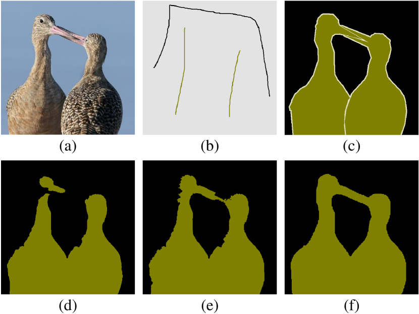
Figure 5: Visualization of the network predictions the corresponding pseudo labels in our training framework. (a) Input image. (b) Sparse annotation. (c) Full annotation. (d) Network prediction. (e) Initial pseudo label generated with the low-level affinity. (f) Final pseudo label generated with multi-level affinities.

Soft Label Assignment. Now that we obtain the pseudo labels, the TEL is designed for soft pseudo label assignment:

$$\mathcal{L}_{tree}=\delta({P},\tilde{Y}),$$ (8)

where $\delta$ is a label assignment function, which measures the distance between predicted probability $P$ and pseudo label $\tilde{Y}$. Some natural choices of $\delta$ can be L1 distance, L2 distance, and so on. We empirically select L1 distance as the label assignment function. For ablations about $\delta$, please refer Sec. 4.4. In this way, the final formation of TEL is described as follows,

$$\mathcal{L}_{tree}=-\frac{1}{|\Omega_{U}|}\sum_{\forall{i}\in\Omega_{U}}|P_{i}-\tilde{Y_{i}}|.$$ (9)

Note that the TEL only focuses on the unlabeled regions since the labeled regions are learned with explicit accurate supervision. Instead of generating pseudo labels from the sparse annotations, our TEL generates the soft labels from network prediction. Thus, the data-driven model learning procedure will benefit our online self-training strategy.

3.4 Discussion

Tree filter has been applied in many vision tasks thanks to the property of structure-preserving. Previous methods apply tree filters to original images for image smoothing [1] and stereo matching [41], or intermediate features for feature transform [26, 25]. Our method is inspired by these works but for a totally different purpose. We capture both low-level and high-level affinities and apply them to network predictions for soft pseudo label generation in SASS, achieving single-stage dynamic online self-training. To the best of our knowledge, it is the first time that the tree filter is introduced in solving the SASS problem.

4 Experiment

Method	Backbone	Publication	Supervision	Multi-stage	Alt. Opt.	Extra Data	CRF	mIoU
(1) DeeplabV2 [4]	VGG16	TPAMI’17	Full	-	-	-	✓	71.6
(2) DeeplabV2 [4]	ResNet101	TPAMI’17	Full	-	-	-	✓	77.7
(3) DeepLabV3+ [5]	ResNet101	ECCV’18	Full	-	-	-	-	80.2
(4) LTF [26]	ResNet101	NeurIPS’19	Full	-	-	-	-	80.9
What’s the point [2]	(1)	ECCV’16	Point	-	-	-	-	43.4
KernelCut Loss [30]	(2)	ECCV’18	Point	✓	-	-	✓	57.0
A2GNN [42]	(2)	TPAMI’21	Point	✓	-	-	✓	66.8
Seminar [3]	(3)	ICCV’21	Point	✓	-	-	-	72.5
SPML [13]	(2)	ICLR’21	Point	-	-	✓	✓	73.2
TEL	(3)	CVPR’22	Point	-	-	-	-	64.9
TEL	(4)	CVPR’22	Point	-	-	-	-	68.4
TEL w. Seminar	(3)	CVPR’22	Point	✓	-	-	-	74.2
ScribbleSup [17]	(1)	CVPR’16	Scribble	✓	✓	-	✓	63.1
NormCut Loss [29]	(2)	CVPR’18	Scribble	✓	-	-	✓	74.5
DenseCRF Loss [30]	(2)	ECCV’18	Scribble	✓	-	-	✓	75.0
KernelCut Loss [30]	(2)	ECCV’18	Scribble	✓	-	-	✓	75.0
GridCRF Loss [20]	(2)	ICCV’19	Scribble	✓	✓	-	-	72.8
BPG [35]	(2)	IJCAI’19	Scribble	-	-	✓	-	76.0
SPML [13]	(2)	ICLR’21	Scribble	-	-	✓	✓	76.1
URSS [22]	(2)	ICCV’21	Scribble	✓	-	-	✓	76.1
PSI [39]	(3)	ICCV’21	Scribble	-	✓	-	-	74.9
Seminar [3]	(3)	ICCV’21	Scribble	✓	-	-	-	76.2
A2GNN [42]	(4)	TPAMI’21	Scribble	✓	-	-	✓	76.2
TEL	(3)	CVPR’22	Scribble	-	-	-	-	77.1
TEL	(4)	CVPR’22	Scribble	-	-	-	-	77.3

Table 1: Experimental results of the point- and the scribble-annotated semantic segmentation methods on the Pascal VOC 2012 validation set. Experimental settings for multi-stage training (Multi-stage), alternating optimization (Alt. Opt.), extra supervised data (Extra Data) during training, and CRF post-processing (CRF) during testing are considered. Top two results are highlighted in blue and red.

4.1 Datasets and Annotations

Datasets. Pascal VOC 2012 [8] contains 20 object categories and a background class. Following previous methods [30, 22, 39, 3], the augmented dataset [11] with 10,582 training and 1,449 validation images are used. Cityscapes [6] is built for urban scenes. It consists of 2,975, 500, 1,525 fine-labeled images for training, validation, and testing, respectively. There are a total of 30 annotated classes in the dataset, and 19 of which are used for semantic segmentation. ADE20k [43] is a challenging benchmarks with 150 fine-grained classes. It collects 20,210, 2,000, and 3,352 images for training, validation, and testing.

Annotations. For point-supervised and scribble-supervised settings, the point-wise annotation [2] and the scribble-wise annotation [17] of Pascal VOC 2012 dataset are respectively used. For the block-supervised setting, we synthesize the block-wise annotations on Cityscapes and the ADE20k datasets. Specially, given the full annotations, we remove the labeled pixels sequentially from semantic edges to interior regions until the ratio of the rest labeled pixels reaches the preset threshold. Examples of synthetic block-wise annotations can be found in our supplementary material.

4.2 Implementation Details

We adopt three popular semantic segmentation models (i.e., the DeeplabV3+ [5], the LTF [26], and the HRNet [28]) for experiments. The ResNet-101 [12] and the HRNetW48 [28] pre-trained on ImageNet [7] dataset are used as backbone networks. For data augmentation, random horizontal flip, random resize in $[0.5,2.0]$, random crop, and random brightness in $[-10,10]$ are employed. The input resolutions are $512\times 512$, $1024\times 512$, and $512\times 512$ for Pascal VOC 2012, Cityscapes, and ADE20k datasets, respectively. And the corresponding initial learning rates are $0.001$, $0.01$, and $0.02$. The SGD optimizer with the momentum of $0.9$, weight decay $1e^{-4}$ polynomial schedule is utilized. The total training iterations are 80k, 40k, and 150k for Pascal VOC 2012, Cityscapes, and ADE20k datasets, respectively. In our practice, we set $\lambda=0.4$ in Eq. 1. As for $\sigma$ in Eq. 5, we set $\sigma=0.02$ in Pascal VOC 2012 dataset, and $\sigma=0.002$ in Cityscapes and ADE20k datasets due to the low-level appearance variety of the semantic categories. All experiments are conducted on Pytorch [23] with 4 Tesla V100 (32G) GPUs.

4.3 Comparison with State-of-the-art Methods

Point-wise supervision. Point-supervised semantic segmentation is an extreme setting in SASS. What’s the Point [2] provides the point-wise annotations for Pascal VOC 2012 dataset. However, it only labels the foreground classes and lacks the annotations of the background class. Following previous works [21, 3], we adopt the point-wise background annotations from the scribble annotations in ScribbleSup [17]. The experimental results are reported in Tab. 1. When equipped with DeeplabV3+, our baseline employing the partial cross-entropy loss can produce 58.5% mIoU. Incorporating the TEL, the segmentation model achieves 6.4% mIoU improvements compared with our baseline. It demonstrates that our method is effective and easy to be plugged into the existing segmentation frameworks. Among recent methods, Seminar [3] has a similar workflow with the semi-supervised mean-teacher method [31] and achieves 72.5% mIoU. We apply our method to the Seminar by replacing the DenseCRF loss with the proposed TEL. It shows that TEL can bring additional 1.7% mIoU improvements and achieve state-of-the-art performance.

Scribble-wise supervision. As shown in Tab. 1, the proposed TEL can be applied in the single-stage training framework and calls for no additional supervised data during training or CRF post-processing during testing. ScribbleSup [17] presents an alternative proposal generation and model training method and achieves 63.1% mIoU. To achieve higher performance, the regularized losses are designed by mining pair-wise relations from low-level image information. BPG [35] and SPML [13] utilize the edge detectors (i.e., the pre-trained HED method [38]) for semantic edge generation and over-segmentation. However, extra supervised data are required to learn the edge detectors. Among all the recent methods, A²GNN achieves the best performance. It first generates seed labels by mixing up multi-level supervisions, then refines the seed labels with affinity attention graph neural networks. Finally, the CRF post-processing is adopted. Compared with A²GNN, our method can be trained in a single-stage manner while outperforming it by 1.1% mIoU without any post-processing.

Fig. 6 illustrates some qualitative results on Pascal VOC 2012 dataset. Although the annotations are quite sparse, our method can leverage the structure information among labeled and unlabeled regions and generate promising masks with fine semantic boundaries.

Block-wise supervision. To further evaluate the robustness of TEL, we carry out additional experiments with block-wise annotations. Notice that the Pascal VOC 2012 dataset is relatively easy since the prediction of pixels close to the semantic boundaries is usually ignored in accuracy calculation (shown in Fig. 2(b)), so we resort to the Cityscapes and the ADE20k datasets. To evaluate the performance with different sparsity, we generate the block-wise annotations at three different levels, including 10%, 20%, and 50% of full labels. The 100% ratio indicates the fully annotated setting, which servers as the upper bound of the SASS methods. The baseline is the segmentation network trained with the partial cross-entropy loss only. We compare our TEL with the state-of-the-art DenseCRF Loss [30] and report the results in Tab. 2. For all block-annotated settings, we use the default hyper-parameters for DenseCRF Loss reported in the paper and it achieves higher accuracy compared with the baseline. However, the performance improvement is relatively limited. The proposed TEL captures both the low-level and the high-level relation and outperforms the DenseCRF Loss in all block-supervised settings.

4.4 Ablation Study

We perform thorough ablation studies for TEL. The scribble-supervised results of DeeplabV3+ on the Pascal VOC 2012 dataset are reported unless otherwise stated.

Loss formation. TEL learns to assign soft labels for unlabeled pixels. The experiments about the loss formation in Eq. 8 are carried out to evaluate the effectiveness of the TEL. The baseline model achieves 68.8% with partial cross-entropy loss. As shown in Tab. 3, the performance can be improved by different formations of TEL. Among them, the L1 distance achieves the best result with 77.1% mIoU, thus we choose it as the final implementation of our TEL.

Model	Backbone	Method	Cityscapes				ADE20k
			10%	20%	50%	100%	10%	20%	50%	100%
HRNet	HRNetW48	Baseline	52.8	58.6	68.8	78.2	30.2	33.1	37.2	42.5
		DenseCRF Loss [30]	57.4	61.8	70.9	-	31.9	33.8	38.4	-
		TEL	61.9	66.9	72.2	-	33.8	35.5	40.0	-
DeeplabV3+	ResNet101	Baseline	48.4	52.8	60.5	80.2	30.8	33.4	36.6	44.6
		DenseCRF Loss [30]	55.6	61.5	69.3	-	31.2	34.0	37.4	-
		TEL	64.8	67.3	71.5	-	34.3	36.0	39.2	-

Table 2: Single-stage training results for block-wise annotations on Cityscapes and ADE20k validation sets.

Formation	Equation	mIoU
Cross Entropy	$-\sum{\tilde{Y}\log{P}}$	76.0
Dot Product	$-\sum{P^{T}\tilde{Y}}$	76.6
L2 Distance	$\sum{{|P-\tilde{Y}|}^{2}}$	75.1
L1 Distance	$\sum{|P-\tilde{Y}|}$	77.1

(a) Ablation of the loss formation for TEL in Eq. 8.

Low-level	High-level	mIoU
		68.8
✓		76.3 (+7.5)
	✓	71.9 (+3.1)
✓	✓	77.1 (+8.3)

(b) Effect of the the low-level and the high-level affinities in TEL.

Information	Method	mIoU
Low-level	BF	75.0
	MST	76.3 (+1.3)
High-level	NL	70.2
	MST	71.9 (+1.7)

(c) Impact of affinity generation methods based on different levels of image information.

Variant	LH-P	HL-C	LH-C
mIoU	76.4	75.8	77.1

(d) Affect of the affinity aggregation strategies.

$\lambda$	0.1	0.2	0.3	0.4	0.5
mIoU	74.9	76.0	76.4	77.1	77.0

(e) Effectiveness evaluation of $\lambda$ in Eq. 1.

$\sigma$	0.01	0.02	0.03	0.04	0.05
mIoU	76.6	77.1	76.8	77.0	76.3

(f) Effectiveness evaluation of $\sigma$ in Eq. 5.

Table 3: Ablation studies on the proposed TEL. We train on the scribble annotations and test on the Pascal VOC 2012 validation set.

Affinity level. The TEL leverage both low-level and high-level structural information to generate pseudo labels for unlabeled pixels. To evaluate their effectiveness, we carry out ablation studies in Tab. 3. Compared with the baseline, introducing low-level and high-level information can achieve 7.5% and 3.1% mIoU improvement, respectively. Adopting both of them, our method achieves 77.1% mIoU, which is 8.3% higher than the baseline.

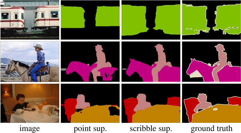
Figure 6: Qualitative results for the proposed TEL on Pascal VOC 2012 dataset. The point sup. and the scribble sup. indicate the point and the scribble supervision, respectively.

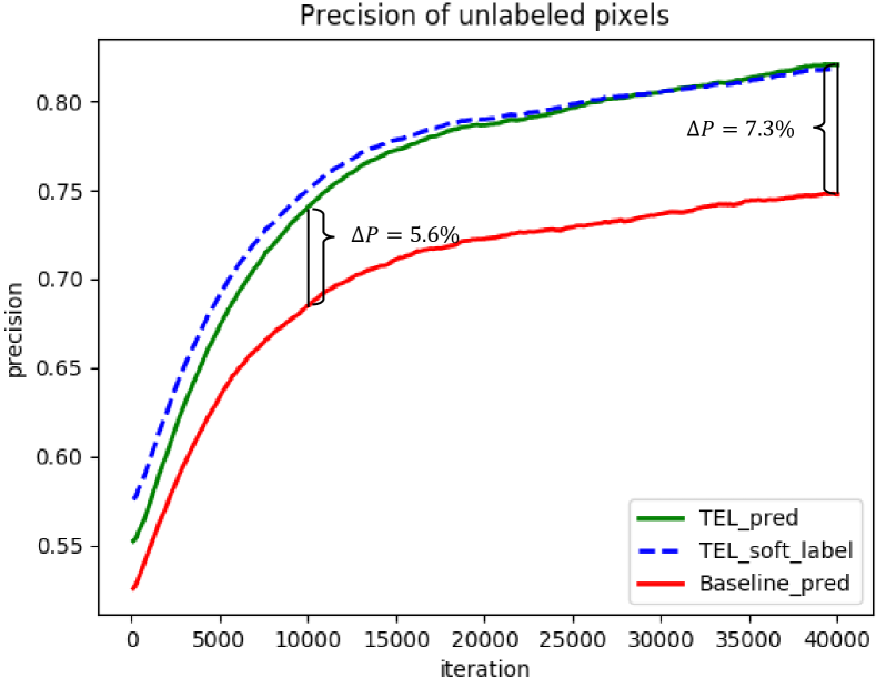
Figure 7: Qualitative evaluation about the network predictions and the soft pseudo labels in unlabeled regions during training. The results of 20% block-wise annotations on Cityscapes are illustrated. ‘TEL_pred’ and ‘TEL_soft_label’ are the network predictions and the generated pseudo labels of the TEL model, respectively. ${\Delta}P$ denotes the precision difference between the baseline training framework and the proposed TEL framework. Extra knowledge can be learned by the segmentation network by incorporating TEL into the baseline.

Affinity generation. The TEL captures the low-level and high-level structural information to generate the affinity matrices in Eq. 5. As shown in Tab. 3, we compare different methods of pair-wise affinity generation, including the Bilateral Filter (BF) for low-level affinity and the Non-Local operation (NL) for high-level affinity. The implementations for BF [30] and NL [37] are adopted. Our method generates affinity matrices based on the MST. Compared with BF, our method requires fewer hyper-parameters while achieving higher accuracy. As for high-level affinity, our method achieves 1.7% higher mIoU than NL. These results demonstrate the effectiveness of TEL in both the low-level and the high-level affinity generation.

Affinity aggregation. How to aggregate the multi-level information is significant to pseudo-label generation. We construct different variants of TEL based on the aggregation strategy. As shown in Tab. 3, LH-P denotes the variant of parallel aggregation. In this case, the low-level and the high-level affinity matrices are multiplied with network predictions separately to produce two pseudo labels, and both of them are used as the guidance for unlabeled pixels. In contrast to the parallel aggregation strategy, the cascading aggregation strategies merge network predictions with the multi-level affinity matrices one by one to refine the pseudo labels sequentially. Among the cascading strategies, we find that aggregating the low-level information first (denoted as LH-C) achieves better results than the variant of aggregating the high-level information first (denoted as HL-C). The low-level affinity is generated from the static color information, which may bring noise due to the inconsistency between low-level color and high-level category information. Incorporating the learnable high-level affinity can improve the semantic consistency.

Hyper-parameters. We evaluate the hyper-parameters of our method, including the $\lambda$ in Eq. 1 and the $\sigma$ in Eq. 5. $\lambda$ is the factor to balance the segmentation loss and TEL. The results are reported in Tab. 3, and we choose $\lambda$ = 0.4 for our TEL. $\sigma$ is a normalization term for the low-level affinity matrix projection. We evaluate the influence of $\sigma$ and report the results in Tab. 3. The value of $\sigma$ is not sensitive to the segmentation accuracy and the highest mIoU is obtained when $\sigma$ equals 0.02 on the Pascal VOC 2012 dataset.

Quality of pseudo labels. We evaluate the quality of pseudo labels for unlabeled pixels on Cityscapes dataset. The baseline segmentation model is HRNet. As shown in Fig. 7, for the model learned with TEL, the precision of the pseudo label is higher than the network prediction at the beginning of the training process, which provides import guidance for model learning. As the number of iterations increases, the precision gap between the prediction and pseudo label is gradually narrowed while the performance of both is improved all the time. Compared with the baseline, TEL can help the segmentation model learn extra knowledge from unlabeled data and achieve performance improvement (from 5.6% to 7.3% mIoU during training).

4.5 Limitations

This paper provides a simple yet effective solution for SASS and achieves state-of-the-art performance. However, it also has some limitations. First, the low-level affinity is generated from the static image, which may bring about noise in the pseudo label. For example, objects with different categories may have similar color information. Second, TEL ignores the inherent relation between the pseudo label and the sparse ground truth. Learning from noise label [10] and alternative optimizer like [20] are possible solutions to solve these problems, respectively.

5 Conclusion

This paper presents a novel tree energy loss (TEL) for sparsely annotated semantic segmentation. The TEL captures both the low-level and the high-level structural information via minimum spanning trees to generate soft pseudo labels for unlabeled pixels, then performs online self-training dynamically. The TEL is effective and easy to be plugged into most of the existing semantic segmentation frameworks. Equipped with the recent segmentation model, our method can be learned in a single-stage manner and outperforms the state-of-the-art methods in point-, scribble-, and block-wise annotated settings without alternating optimization procedures, extra supervised data, or time-consuming post-processes.

Appendix A Failure cases

Fig. 8 shows some failure cases of our method. The predictive error occurs due to the color mutation within one object region or the color similarity between two semantic objects. Since our approach partially relies on the low-level color prior to generate the pseudo labels, so it may make wrong predictions under point-wise supervision. Fortunately, the predictive error can be reduced by introducing more complete annotations (i.e., scribble annotation).

Appendix B Computational costs

The proposed method can be plugged into most existing semantic segmentation frameworks. During inference, the auxiliary branch can be removed. During training, the GPU loads and the training time evaluation on Pascal VOC 2012 dataset are reported in Tab. 4 and Tab. 5, respectively. The DeeplabV3+ [5] and the LTF [26] are selected as the baselines. The resolution of the input image is $512\times 512$ and the batch size is 16. The two MST affinities are derived on the resolution of network predictions (e.g., 4 times smaller than the input resolution). Leveraging the low-level information almost introduces no extra memory cost while introducing both low-level and high-level information requires 5.88% and 3.82% GB GPU loads for DeeplabV3+ and LTF models, respectively. The training time of our method only increases around 9% compared to the baseline.

Appendix C Comparison to the naive online self-training

The proposed TEL leverages the multi-level structural information to dynamically generated the pseudo labels for unlabeled pixels, achieving online self-training at the training stage. As shown in Tab. 6, compared to the naive online self-training strategy which adopts a preset threshold to binary the pseudo labels, our TEL surpasses it with large improvements.

Appendix D Experiments on Pascal VOC 2012 test set

The scribble-supervised experimental results on Pascal VOC 2012 test set are reported in Tab. 7. Since the quality of pseudo labels is based on network predictions in our method, advanced backbones are helpful to fully explore the effectiveness of TEL. To evaluate the performance with simpler models, we also report the results of DeeplabV2 backbone. Our TEL is clean and outperforms the multi-stage method A²GN by more than 1% mIoU as well.

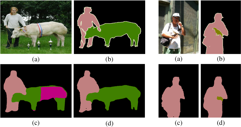
Figure 8: Failure cases of the proposed method on Pascal VOC 2012 dataset [8]. (a) input image. (b) ground truth. (c) result with point-wise supervision. (d) result with scribble-wise supervision.

Low-level	High-level	DeeplabV3+	LTF
		32.85	46.65
✓		32.86 (+0.03%)	46.67 (+0.04%)
✓	✓	34.78 (+5.88%)	48.43 (+3.82%)

Table 4: The memory cost (GB) during training, leveraging various levels of structural information.

Low-level	High-level	DeeplabV3+	LTF
		9.0	11.7
✓		9.2 (+2.2%)	12.2 (+4.3%)
✓	✓	9.8 (+8.9%)	12.7 (+8.5%)

Table 5: The training time (hour) evaluation of our method, leveraging various levels of structural information.

Threshold	0.5	0.6	0.7	0.8	0.9	0.95	1.0
mIoU	7.3	7.3	7.5	56.5	70.2	70.3	68.8

Table 6: The scribble-annotated experiments about naive online self-training on VOC 2012 val set. The threshold 1.0 means the original baseline without pseudo-label supervision.

Method	Backbone	Multi-stage	Extra Data	CRF	mIoU
SPML (ICLR’21)	DeeplabV2	-	✓	✓	76.4
A2GNN (TPAMI’21)	DeeplabV2	✓	-	✓	74.0
A2GNN (TPAMI’21)	LTF	✓	-	✓	76.1
TEL	DeeplabV2	-	-	-	74.8
TEL	DeeplabV2	-	-	✓	76.0
TEL	LTF	-	-	-	77.5

Table 7: Experimental results of the scribble-annotated semantic segmentation methods on the Pascal VOC 2012 test set.

Appendix E Visualizations of block-supervised settings

We synthesize the block-wise annotations for ADE20k [43] and Cityscapes [6] datasets. Given the full annotations of the image, we discard the annotations from the semantic boundary to the interior region until the ratio of the rest annotations reaches the preset threshold. The block-wise annotations are generated at 3 levels, including 10%, 20%, and 50% of full annotations. The visualizations of block-wise annotation for the two datasets are respectively illustrated in Fig. 9 and Fig. 10. Moreover, qualitative results of our method on the ADE20k and the Cityscapes datasets are illustrated in Fig. 11 and Fig. 12, respectively. Here, HRNet is selected as the segmentation model. The proposed approach can be used to train the segmentation model with the annotations of different sparsity.

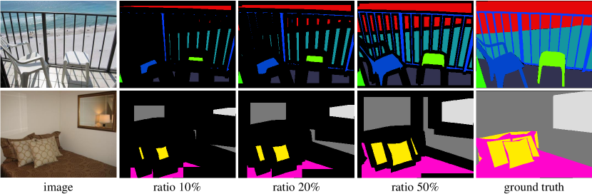
Figure 9: The block-wise annotations for ADE20k dataset.

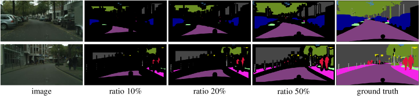
Figure 10: The block-wise annotations for Cityscapes dataset.

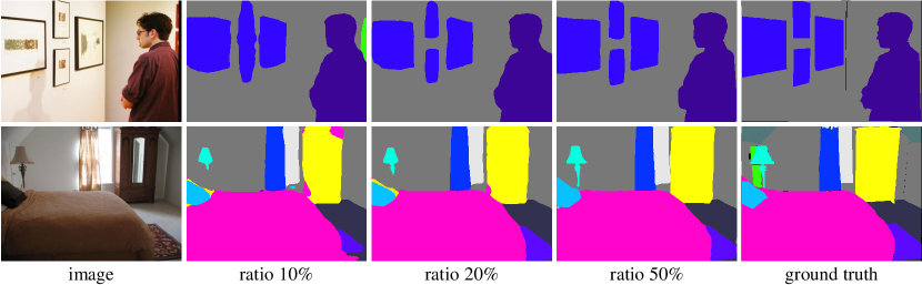
Figure 11: Qualitative results for the proposed TEL on ADE20k dataset.

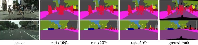
Figure 12: Qualitative results for the proposed TEL on Cityscapes dataset.

References

- [1] Linchao Bao, Yibing Song, Qingxiong Yang, Hao Yuan, and Gang Wang. Tree filtering: Efficient structure-preserving smoothing with a minimum spanning tree. TIP, 23(2):555–569, 2013.
- [2] Amy Bearman, Olga Russakovsky, Vittorio Ferrari, and Li Fei-Fei. What’s the point: Semantic segmentation with point supervision. In ECCV, 2016.
- [3] Hongjun Chen, Jinbao Wang, Hong Cai Chen, Xiantong Zhen, Feng Zheng, Rongrong Ji, and Ling Shao. Seminar learning for click-level weakly supervised semantic segmentation. In ICCV, 2021.
- [4] Liang-Chieh Chen, George Papandreou, Iasonas Kokkinos, Kevin Murphy, and Alan L Yuille. Deeplab: Semantic image segmentation with deep convolutional nets, atrous convolution, and fully connected crfs. TPAMI, 40(4):834–848, 2017.
- [5] Liang-Chieh Chen, Yukun Zhu, George Papandreou, Florian Schroff, and Hartwig Adam. Encoder-decoder with atrous separable convolution for semantic image segmentation. In ECCV, 2018.
- [6] Marius Cordts, Mohamed Omran, Sebastian Ramos, Timo Rehfeld, Markus Enzweiler, Rodrigo Benenson, Uwe Franke, Stefan Roth, and Bernt Schiele. The cityscapes dataset for semantic urban scene understanding. In CVPR, 2016.
- [7] Jia Deng, Wei Dong, Richard Socher, Li-Jia Li, Kai Li, and Li Fei-Fei. Imagenet: A large-scale hierarchical image database. In CVPR, 2009.
- [8] Mark Everingham, Luc Van Gool, Christopher KI Williams, John Winn, and Andrew Zisserman. The pascal visual object classes (voc) challenge. IJCV, 88(2):303–338, 2010.
- [9] Robert G. Gallager, Pierre A. Humblet, and Philip M. Spira. A distributed algorithm for minimum-weight spanning trees. TOPLAS, 5(1):66–77, 1983.
- [10] Bo Han, Quanming Yao, Xingrui Yu, Gang Niu, Miao Xu, Weihua Hu, Ivor Tsang, and Masashi Sugiyama. Co-teaching: Robust training of deep neural networks with extremely noisy labels. In NeurIPS, 2018.
- [11] Bharath Hariharan, Pablo Arbeláez, Lubomir Bourdev, Subhransu Maji, and Jitendra Malik. Semantic contours from inverse detectors. In ICCV, 2011.
- [12] Kaiming He, Xiangyu Zhang, Shaoqing Ren, and Jian Sun. Deep residual learning for image recognition. In CVPR, 2016.
- [13] Tsung-Wei Ke, Jyh-Jing Hwang, and Stella X Yu. Universal weakly supervised segmentation by pixel-to-segment contrastive learning. In ICLR, 2021.
- [14] Takanori Koga and Noriaki Suetake. Structural-context-preserving image abstraction by using space-filling curve based on minimum spanning tree. In ICIP, 2011.
- [15] Jae-Hun Lee, ChanYoung Kim, and Sanghoon Sull. Weakly supervised segmentation of small buildings with point labels. In ICCV, 2021.
- [16] Stan Z Li. Markov random field models in computer vision. In ECCV, 1994.
- [17] Di Lin, Jifeng Dai, Jiaya Jia, Kaiming He, and Jian Sun. Scribblesup: Scribble-supervised convolutional networks for semantic segmentation. In CVPR, 2016.
- [18] Chenxi Liu, Liang-Chieh Chen, Florian Schroff, Hartwig Adam, Wei Hua, Alan L Yuille, and Li Fei-Fei. Auto-deeplab: Hierarchical neural architecture search for semantic image segmentation. In CVPR, 2019.
- [19] Peidong Liu, Zibin He, Xiyu Yan, Yong Jiang, Shu-Tao Xia, Feng Zheng, and Hu Maowei. Weclick: Weakly-supervised video semantic segmentation with click annotations. In ACM MM, 2021.
- [20] Dmitrii Marin, Meng Tang, Ismail Ben Ayed, and Yuri Boykov. Beyond gradient descent for regularized segmentation losses. In CVPR, 2019.
- [21] Anton Obukhov, Stamatios Georgoulis, Dengxin Dai, and Luc Van Gool. Gated crf loss for weakly supervised semantic image segmentation. arXiv preprint arXiv:1906.04651, 2019.
- [22] Zhiyi Pan, Peng Jiang, Yunhai Wang, Changhe Tu, and Anthony G Cohn. Scribble-supervised semantic segmentation by uncertainty reduction on neural representation and self-supervision on neural eigenspace. In ICCV, 2021.
- [23] Adam Paszke, Sam Gross, Francisco Massa, Adam Lerer, James Bradbury, Gregory Chanan, Trevor Killeen, Zeming Lin, Natalia Gimelshein, Luca Antiga, et al. Pytorch: An imperative style, high-performance deep learning library. In NeurIPS, 2019.
- [24] Rui Qian, Yunchao Wei, Honghui Shi, Jiachen Li, Jiaying Liu, and Thomas Huang. Weakly supervised scene parsing with point-based distance metric learning. In AAAI, 2019.
- [25] Lin Song, Yanwei Li, Zhengkai Jiang, Zeming Li, Xiangyu Zhang, Hongbin Sun, Jian Sun, and Nanning Zheng. Rethinking learnable tree filter for generic feature transform. In NeurIPS, 2020.
- [26] Lin Song, Yanwei Li, Zeming Li, Gang Yu, Hongbin Sun, Jian Sun, and Nanning Zheng. Learnable tree filter for structure-preserving feature transform. In NeurIPS, 2019.
- [27] Jean Stawiaski and Fernand Meyer. Minimum spanning tree adaptive image filtering. In ICIP, 2009.
- [28] Ke Sun, Yang Zhao, Borui Jiang, Tianheng Cheng, Bin Xiao, Dong Liu, Yadong Mu, Xinggang Wang, Wenyu Liu, and Jingdong Wang. High-resolution representations for labeling pixels and regions. arXiv preprint arXiv:1904.04514, 2019.
- [29] Meng Tang, Abdelaziz Djelouah, Federico Perazzi, Yuri Boykov, and Christopher Schroers. Normalized cut loss for weakly-supervised cnn segmentation. In CVPR, 2018.
- [30] Meng Tang, Federico Perazzi, Abdelaziz Djelouah, Ismail Ben Ayed, Christopher Schroers, and Yuri Boykov. On regularized losses for weakly-supervised cnn segmentation. In ECCV, 2018.
- [31] Antti Tarvainen and Harri Valpola. Mean teachers are better role models: Weight-averaged consistency targets improve semi-supervised deep learning results. NeurIPS, 30, 2017.
- [32] Zhi Tian, Chunhua Shen, Xinlong Wang, and Hao Chen. Boxinst: High-performance instance segmentation with box annotations. In CVPR, 2021.
- [33] Wei-Chih Tu, Shengfeng He, Qingxiong Yang, and Shao-Yi Chien. Real-time salient object detection with a minimum spanning tree. In CVPR, 2016.
- [34] Paul Vernaza and Manmohan Chandraker. Learning random-walk label propagation for weakly-supervised semantic segmentation. In CVPR, 2017.
- [35] Bin Wang, Guojun Qi, Sheng Tang, Tianzhu Zhang, Yunchao Wei, Linghui Li, and Yongdong Zhang. Boundary perception guidance: a scribble-supervised semantic segmentation approach. In IJCAI, 2019.
- [36] Wenguan Wang, Tianfei Zhou, Fisher Yu, Jifeng Dai, Ender Konukoglu, and Luc Van Gool. Exploring cross-image pixel contrast for semantic segmentation. In ICCV, 2021.
- [37] Xiaolong Wang, Ross Girshick, Abhinav Gupta, and Kaiming He. Non-local neural networks. In CVPR, 2018.
- [38] Saining Xie and Zhuowen Tu. Holistically-nested edge detection. In ICCV, 2015.
- [39] Jingshan Xu, Chuanwei Zhou, Zhen Cui, Chunyan Xu, Yuge Huang, Pengcheng Shen, Shaoxin Li, and Jian Yang. Scribble-supervised semantic segmentation inference. In ICCV, 2021.
- [40] Qingxiong Yang. A non-local cost aggregation method for stereo matching. In CVPR, 2012.
- [41] Qingxiong Yang. Stereo matching using tree filtering. TPAMI, 37(4):834–846, 2014.
- [42] Bingfeng Zhang, Jimin Xiao, Jianbo Jiao, Yunchao Wei, and Yao Zhao. Affinity attention graph neural network for weakly supervised semantic segmentation. TPAMI, 2021.
- [43] Bolei Zhou, Hang Zhao, Xavier Puig, Sanja Fidler, Adela Barriuso, and Antonio Torralba. Scene parsing through ade20k dataset. In CVPR, 2017.
- [44] Tianfei Zhou, Liulei Li, Xueyi Li, Chun-Mei Feng, Jianwu Li, and Ling Shao. Group-wise learning for weakly supervised semantic segmentation. TIP, 31:799–811, 2021.
- [45] Tianfei Zhou, Meijie Zhang, Fang Zhao, and Jianwu Li. Regional semantic contrast and aggregation for weakly supervised semantic segmentation. In CVPR, 2022.