Better Language Model with Hypernym Class Prediction
Abstract
Class-based language models (LMs) have been long devised to address context sparsity in -gram LMs. In this study, we revisit this approach in the context of neural LMs. We hypothesize that class-based prediction leads to an implicit context aggregation for similar words and thus can improve generalization for rare words. We map words that have a common WordNet hypernym to the same class and train large neural LMs by gradually annealing from predicting the class to token prediction during training. Empirically, this curriculum learning strategy consistently improves perplexity over various large, highly-performant state-of-the-art Transformer-based models on two datasets, WikiText-103 and arXiv. Our analysis shows that the performance improvement is achieved without sacrificing performance on rare words. Finally, we document other attempts that failed to yield empirical gains, and discuss future directions for the adoption of class-based LMs on a larger scale.
1 Introduction
Over the course of the past decades, language modeling (LM) has transitioned from -gram to neural models (Bengio et al., 2003; Mnih and Hinton, 2007; Devlin et al., 2019; Brown et al., 2020). Performance improvement of today’s neural LMs is often achieved at the cost of increased computational resources. For example, to capture long-term dependencies, various extensions of Transformer-based LMs have been proposed (Dai et al., 2019; Rae et al., 2020). These modifications bring about significant improvements on held-out perplexity, but training cost also increases significantly due to large GPU memory consumption and more computations at each training step.
In parallel, alternative training strategies have also been proposed Guu et al. (2020); Ziegler and Rush (2019); Deng et al. (2020). In this paper, we explore the effectiveness of class-based language models (CLMs, Brown et al. 1992) in the context of neural LMs. CLMs group individual words into coarser-grained classes and has proven effective in alleviating context sparsity in -gram LMs (Dagan et al., 1999). It has been also used to improve computational efficiency in neural LMs (Morin and Bengio, 2005; Grave et al., 2017a). More recently, Levine et al. (2020) pretrain masked LMs Devlin et al. (2019) by predicting WordNet supersense labels. However, the work focuses on word-sense disambiguation tasks and doesn’t provide clear evidence of gains in terms of perplexity.
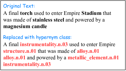
In this paper, we revisit CLM and assign words to classes by leveraging hypernym relations from the WordNet (Miller, 1995). Our proposal, dubbed Hypernym Class Prediction (HCP) is simple and effective: for each batch, we substitute a subset of the tokens with their WordNet hypernyms (see Figure 1). Then, we train an autoregressive LM on the resulting sentences using a mixed vocabulary composed of hypernyms and tokens. Crucially, we anneal the substitution rate during training, i.e., we gently switch from hypernym prediction to token prediction, following a curriculum learning approach. Note that this approach does not require WordNet information at inference time nor increases training time.
Our approach is motivated by two hypotheses. Firstly, mapping words to their hypernyms gives rise to a natural gradation of difficulty in the prediction task. Prior work has shown that LM benefits from training on instances of increasing difficulty (Bengio et al., 2009; Press et al., 2021). We thus postulate that, when coupled with the right curriculum, HCP can improve LM training and perplexity. Secondly, we hypothesize that HCP can improve rare word generalization through implicit context sharing. Neural models still struggle to learn reliable representations for rare words Schick and Schütze (2020). With CLM-based models, data sparsity for rare words can be abated, e.g., when the representation of their contexts are potentially drawn closer to those of their more frequent siblings by way of label (hypernym) sharing.
Empirically, the proposed method consistently yields about 0.6–1.9% relative reduction in perplexity over baselines on the WikiText-103 dataset Merity et al. (2016), and 1.3–3.1% on the arXiv dataset Lazaridou et al. (2021). These improvements are observed with respect to memory-augmented Dai et al. (2019) and segment-aware Bai et al. (2021) LMs. Importantly, the proposed method improves performance for both rare and frequent words. We also observe that this is in contrast with performance improvements in regular LMs, which seem to be achieved at the cost of worsened performance on rare words.
To the best of our knowledge, this is the first work that shows how perplexity of Transformer LMs can be improved by leveraging hypernymy relationships. We provide an extensive ablation study highlighting crucial elements of HCP. Amongst those, we found particularly important to adopt a curriculum learning approach, rather than multi-objective learning or adaptive-softmax, and excluding frequent words from the hypernym prediction task. We highlight the simplicity and effectiveness of the proposed method as our main contribution, and hope this study would facilitate further exploration in this line of research.
2 Related Work
Transformer-based models are now popular language models. Dai et al. (2019) propose Transformer-XL by extending the vanilla Transformer Vaswani et al. (2017) with a memory segment, which can encode more context tokens to predict the next token. Rae et al. (2020) extend Transformer-XL with a compressed memory segment to further encode long-time context memory. Other works explore different sparse Transformers to encode much longer sequences for LM Beltagy et al. (2020); Roy et al. (2021). Bai et al. (2021) propose a segment-aware Transformer (Segatron) to encode more positional information for language modeling. Despite their effectiveness, neural models still struggle to learn reliable representations for rare words. Some approaches have been proposed to tackle this challenge by way of morphology (Luong et al., 2013), lexical similarity (Khassanov et al., 2019), context similarity (Schick and Schütze, 2020; Khandelwal et al., 2020) and tokenization (Kudo and Richardson, 2018).
In addition to the model modifications, other work investigated curriculum learning to train LMs. Bengio et al. (2009) first find that curriculum learning could benefit LM training by training with high-frequency tokens first and low-frequency tokens later. Wu et al. (2021) find that curricula works well when the training data is noisy or the training data is too large to iterate multiple epochs. Press et al. (2021) find that training Transformer-based LMs with short sequences first could improve convergence speed and perplexity.
Related work aimed at integrating WordNet information into pretrained language models. Levine et al. (2020) propose SenseBERT by adding the word sense (WordNet supersense) prediction as an additional task during BERT Devlin et al. (2019) pre-training. SenseBERT outperforms BERT on both word supersense disambiguation Raganato et al. (2017) task and word in context Pilehvar and Camacho-Collados (2019) task. Recently, Porada et al. (2021) use WordNet hypernymy chains as input to a Roberta Liu et al. (2019) model to predict the plausibility of input events. In this work, our focus is to improve performance of auto-regressive LMs. We show that a multi-task strategy harms performance in this setting, and give a successful recipe to consistently boost LM performance with class-based predictions.
3 Method
Coupling class-based LM (CLM) and curriculum learning, HCP is to gradually anneal class prediction to token prediction during LM training. In this section, we first describe how we instantiate word classes by leveraging hypernym relation from the WordNet. We then present how to incorporate the proposed Hypernym Class Prediction task into LM training via curriculum learning.
3.1 Hypernymy as Word Classes
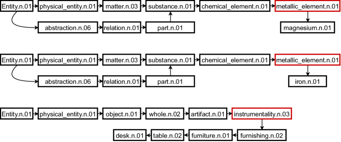
WordNet Miller (1995) is a lexical database that groups words into sets of cognitive synonyms known as synsets, which are in turn organized into a directed graph by various lexical relations including the hypernymy (is-a) relation. As shown in Figure 2, each vertex is a synset, labeled by the text within the box, and each edge points from the hypernym (supertype) to the hyponym (subtype). Note that a word form (spelling) may be associated with multiple synsets – each corresponding to a different sense of the word, which are sorted by the frequency of the sense estimated from a sense-annotated corpus. For example, iron has 6 synsets, among which “iron.n.01” is the most common one.
Hence, if two words share the same hypernym at a certain level in their hypernym-paths (to the root in WordNet), we could say they are similar at that level. Here we use "Depth" to quantify the hypernym-path level. In Figure 2, for example, at Depth 6, iron and magnesium are mapped to the same group named “metallic_element.n.01”, while desk is mapped to “instrumentality.n.03”. At Depth 2, all these three words share the same (indirect) hypernym “physical_entity.n.01”.
In this work, we map each token in our training set into its hypernym class if this token (1) has a noun synset in the WordNet, (2) with a hypernym-path longer than a given depth , and (3) has frequency below a given threshold in the training corpus. We only consider nouns because it is not only the most common class in the WordNet but also a difficult class for LMs to learn Lazaridou et al. (2021). For tokens with multiple synsets, we iterate over the synsets in the order of sense frequency and break the loop once found. We select the most frequent synset no less than the required depth. The mapping pseudocode is illustrated in Code 1, which is a data pre-processing algorithm conducted only once before the training and takes no more than 5 minutes in our implementation.
3.2 Hypernym Class Prediction
We first partition the vocabulary into and based on whether or not a token has a hypernym in the WordNet, and denotes the set of all hypernyms. The original task in a Transformer-based LM is then to predict the token ’s probability with the output from the last layer:
| (1) |
where is the word in the original vocabulary and is its embedding. Here we assume the output layer weights are tied with the input embeddings. We call any training step predicted with Eq. 1 a token prediction step.
To do the Hypernym Class Prediction step, we replace all tokens in in a batch of training data with their corresponding hypernym classes in . After the replacement, only hypernym classes in and tokens in can be found in that batch. Then, the LM probability prediction becomes:
| (2) |
where could be either a token or a hypernym class. We called this batch step is a Hypernym Class Prediction (HCP) step.
Note that Eq. 2 is different from the multi-objective learning target, where the hypernym class would be predicted separately:
| (3) |
where is a hypernym class. We will elaborate on this difference in the experiment results part.
3.3 Training Method
We train a LM by switching from HCP to token prediction. For the example in Figure 2, our target is to teach a model to distinguish whether the next token belongs to the metallic element class or instrumentality class during the earlier stage in training, and to predict the exact word from magnesium, iron, and desk later.
Inspired by Bengio et al. (2009), we choose curriculum learning to achieve this. Curriculum learning usually defines a score function and a pacing function, where the score function maps from a training example to a difficulty score, while the pacing function determines the amount of the easiest/hardest examples that will be added into each epoch. We use a simple scoring function which treats HCP as an easier task than token prediction. Therefore, there is no need to sort all training examples. The pacing function determines whether the current training step is a HCP step, i.e. whether tokens will be substituted with their hypernyms.
Our pacing function can be defined as:
| (4) |
or
| (5) |
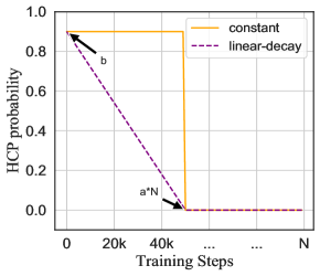
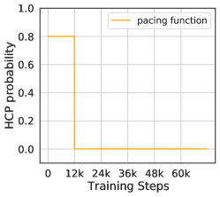
where is the probability that the current step is a hypernym class prediction step. is the total training steps. and are hyper-parameters. So, Eq. 4 is a constant pacing function in the first steps, while Eq. 5 is a linear decay function. We plot these two functions in Figure 3. According to our experimental results Tab. 5, these two functions are both effective in improving the language model.
| Model | #Param. | Valid PPL | Test PPL |
|---|---|---|---|
| LSTM+Neural cache Grave et al. (2017b) | - | - | 40.8 |
| Transformer small | 91M | 34.5 | 36.5 |
| + HCP | 34.1 | 35.9 | |
| Transformer base | 151M | 29.2 | 30.7 |
| + HCP | 29.1 | 30.2 | |
| Transformer-XL base, M=150 Dai et al. (2019) | 151M | - | 24.0 |
| Segatron-XL base Bai et al. (2021), M=150 | 151M | - | 22.5 |
| + HCP | 21.9 | 22.1 | |
| Transformer Large | 257M | 24.0 | 25.8 (80k steps) |
| + HCP | 23.7 | 25.3 (80k steps) | |
| Adaptive Input Baevski and Auli (2019) | 247M | - | 18.7 (286k steps) |
| Transformer-XL large, M=384 Dai et al. (2019) | 257M | - | 18.3 (400k steps) |
| Compressive Transformer, M=1024 Rae et al. (2020) | 257M | 16.0 | 17.1 (400k steps) |
| Segatron-XL large, M=384 Bai et al. (2021) | 257M | - | 17.1 (350k steps) |
| + HCP | 16.1 | 17.0 (350k steps) |
4 Experiments
We conduct experiments on two datasets. WikiText-103 Merity et al. (2016) is a large word-level dataset with long-distance dependencies for language modeling. There are 103M tokens and 28K articles (3.6K tokens per article on average). The original vocabulary size is 271121, among which we find 3383 hypernym classes for 71567 tokens with and (Section 3.1). arXiv Lazaridou et al. (2021) is collected from publicly available arXiv abstracts111https://arxiv.org/help/oa/index with an average of 172 words per abstract and partitioned into training (1986–Sept 2017), evaluation (Aug–Dec 2017), and test (2018–2019). Following Lazaridou et al. (2021), we use the BPE Sennrich et al. (2015) tokenization for this dataset. The final vocabulary size is 48935, and we find 1148 hypernym classes for 5969 tokens among the vocabulary with and .
Several variants of the Transformer model have been used for our experiments:
-
•
small model: 12 layers, 10 heads, hidden size 300, batch size 256, training steps 100k;
-
•
base model: 16 layers, 10 heads, hidden size 410, batch size 64, training steps 200k;
-
•
large model: 18 layers, 16 heads, hidden size 1024 batch size 128.
The input lengths are 150 for the base model and 384 for the large model. The memory length is equal to the input length for both training and testing. The hyper-parameters used for the arXiv dataset are as same as the WikiText-103, except the arXiv base model’s input length is 384. The number of training steps varies greatly for the large model in previous work, so we experiment on both the lower (80k) higher (350k) ends.
4.1 Main results
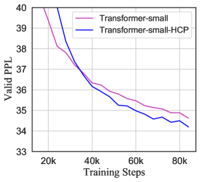
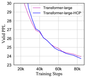
Our main results are shown in Table 1. We can see that all architectures could benefit from HCP: Transformer-small improved 0.6 ppl, Transformer-base improved 0.5, Segatron-XL base improved 0.4, Transformer-large improved 0.5, and Segatron-XL large improved 0.1. We also plot the validation perplexities of small and large models trained with and without HCP in Figure 4. In the beginning, the perplexity of the HCP models is higher due to the mixed training steps from the two tasks, but we can see that HCP perplexity goes down faster than the baseline method. And after fully switching to token prediction, HCP outperforms the baseline method quickly and the gap between these two methods remains stable. These results suggest that HCP is indeed effective in improving LM training.
| Model | #Param. | Valid PPL | Test PPL |
|---|---|---|---|
| Segatron-XL base | 59M | 22.39 | 24.21 |
| + HCP | 21.79 | 23.46 | |
| Transformer-XL large Lazaridou et al. (2021) | 287M | - | 23.07 |
| Segatron-XL large | 283M | 21.28 | 22.99 (80k steps) |
| + HCP | 283M | 20.93 | 22.60 (80k steps) |
For experiments on the arXiv dataset, we first compare the Segatron-XL base model trained with and without HCP. The results are shown in Table 2. The improvements over the validation set and test set are 0.6 and 0.75 respectively. For the large model, we use the same model architecture and hyper-parameters as the WikiText-103 large model but change the vocabulary to BPE sub-tokens. The final perplexity outperforms its counterparts about 0.4 and outperforms a larger model trained with 1024 input sequence length over 0.47, while our model length is 384.
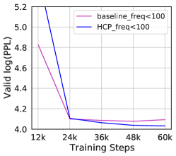
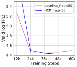
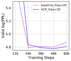
4.2 Generalization on Rare Tokens
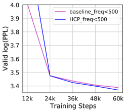
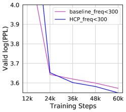
In addition to the overall perplexity comparison, we also conduct comparisons with frequency-stratified validation subsets, to show the perplexity of tokens that has been replaced with the hypernym classes during training. Results are shown in Figure 5. We can see that, after the first 12k hypernym class prediction steps, there is a large gap between our HCP model and the baseline model as the HCP model only learn to predict the hypernym class instead of the token itself. After that, in the next 12k steps, HCP’s PPL decreases faster, achieves similar PPL at 24k steps, and finally outperforms the baseline method in all frequency groups. The results show that our proposed training method can benefit the learning of the replaced tokens in various frequencies. Strikingly, we observe that, for the baseline, more training steps lead to a degradation of performance for rare tokens, a behavior that deserves investigation in future work.
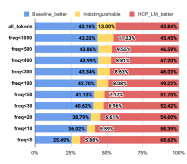
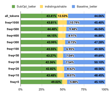
We further conduct pairwise model comparisons with tokens that have been replaced during HCP training on the WikiText-103 test set. Given two models, we compare the prediction probabilities for each occurrence of a target token, and register a “win” for the model with a higher probability. We then calculate the percentage of winnings (as well as ties) for each model by tallying over all occurrences of the token. The results are then stratified by token frequency and plotted in Figure 6. The better model is placed on the right in both sub-figures.
In Figure 6(a), we see that HCP outperforms the baseline model on all frequency strata. Interestingly, the performance gap widens as frequency decreases, indicating that HCP is beneficial in modeling rare tokens. In Figure 6(b), we compare the baseline model against an under-optimized model of identical architecture but slightly different hyper-parameters.222The sub-optimal model has batch size 128 instead of the optimal 64, and the perplexity gap between these two models is observed to be slightly larger than that between HCP and the baseline (0.9 vs 0.5). Here, the (optimal) baseline outperforms the sub-optimal model on all but the least frequent stratum, suggesting the possibility that perplexity reduction (resulting from hyperparameter tuning in this case) might be achieved by improving frequent word prediction at the expense of rare words. This is inline with observations made recently in vision tasks (Sagawa et al., 2020).
4.3 Ablation study
We conduct ablation studies with WikiText-103 dataset and Transformer small model to investigate how to map words to hypernym classes, how to select curriculum learning pacing functions and to show why we use curriculum training.
4.3.1 Hypernym-path Depth
The hypernym classes are chosen from the hypernym-paths in WordNet. Considering that a hypernym-path consists of multiple hypernyms, it is not straightforward to tell which layer is the best. But the best depth should be some layer in the middle. Because a small depth might map multiple distant words into the same class, while a large depth will result in too many classes which are hard for a model to learn. The extreme examples could be and , corresponding to mapping all candidate words into the class “Entity.n.01” and mapping each word into itself respectively. In Table 3, we show evaluation results among different depth selections. We find that depth 6th is the best choice, with the lowest valid perplexity. The results also confirm our assumption that the best one would be some middle layer.
| Depth | Valid PPL | #Classes |
|---|---|---|
| Baseline | 34.5 | 0 |
| 34.54 | 145 | |
| 34.29 | 1169 | |
| 34.05 | 3383 | |
| 34.37 | 6604 | |
| 34.25 | 9063 |
4.3.2 Filter Frequency
In addition to the hypernym-path depth, we also investigate how to select frequency threshold . As we mentioned above, our target is to map similar words into the same class, where predicting a hypernym class might be easier than predicting multiple different words. After the mapping process, low-frequency words can be clustered into hypernym classes with higher frequency. Table 4 shows the results of different . We can see that achieves the best results while (without filter) is the worst. We hypothesize this might be due to two reasons. First, for some high-frequency common words, the model can learn them well already, while mapping them into hypernym classes may be superfluous or even harmful. Second, including frequent words skews the marginal distribution over hypernym classes, causing hypernym prediction to be more class-imbalanced, which in turn might lead to collapsed representation in the resulting LM Fang et al. (2021). This hypothesis deserves further investigation. It should be noted that although the difference of #Rep.Tokens looks minor, the difference in the token’s appearance is significant. For example, maps only 776 additional tokens compared with , but each token’s appearance is more than 8000, which explains the different perplexities in Table 4.
| FilterFreq. | Valid PPL | #Rep. |
|---|---|---|
| Baseline | 34.5 | 0 |
| 34.14 | 70859 | |
| 34.50 | 71735 | |
| 34.05 | 71971 | |
| 34.32 | 72153 | |
| 34.35 | 72291 | |
| 40.10 | 73067 |
| Constant Func. | HCP steps | Valid PPL | NonRep.PPL | Rep.PPL | |
|---|---|---|---|---|---|
| a=0 b=0 | 0 | 34.5 | 22.07 | 348.87 | |
| a=0.1 b=1 | 10k | 34.18 | 22.08 | 339.30 | |
| a=0.2 b=1 | 20k | 34.15 | 22.07 | 339.34 | |
| a=0.3 b=1 | 30k | 34.26 | 22.07 | 338.14 | |
| a=0.4 b=1 | 40k | 34.39 | 22.26 | 338.31 | |
| Linear Func. | |||||
| a=0.45 b=0.45 | 10k | 34.14 | 22.04 | 340.55 | |
| a=0.64 b=0.64 | 20k | 34.05 | 21.96 | 341.33 | |
| a=0.78 b=0.78 | 30k | 34.26 | 22.05 | 346.77 | |
| a=0.90 b=0.90 | 40k | 34.56 | 22.12 | 354.40 |
| Valid PPL | Test PPL | NonRep.PPL | Rep.PPL | |
|---|---|---|---|---|
| Baseline | 34.50 | 36.46 | 22.07 | 348.87 |
| Adaptive Softmax | 36.32 | 38.16 | 22.48 | 435.93 |
| Multi-obj | ||||
| last layer | 46.06 | 48.49 | 27.81 | 627.23 |
| 8th layer | 43.42 | 45.37 | 26.13 | 597.66 |
| 8th layer + mix vocab | 35.97 | 38.02 | 22.98 | 365.27 |
| Hypernym Class Prediction | 34.05 | 35.87 | 21.96 | 341.33 |
4.3.3 Pacing Function
Table 5 shows the results of models trained with various curriculum pacing functions. We also report the validation perplexities of the tokens that have ever been replaced with hypernym class (Rep.PPL) during training and tokens without hypernym class (NonRep.PPL).
For the constant pacing function, we fix and change the value of , In this case, the models are always training with HCP in the first steps and then switch to the token prediction training, which is a pre-training pacing function. We can see that all models outperform the baseline model over the validation perplexity. Rep.PPL improves from 348 to 339. The perplexity of NonRep.PPL between baseline model and HCP models are similar, except the model trained with , which indicates the pre-training should not take up too many steps.
For the linear pacing function, we choose some specific and to achieve the same HCP steps as the constant functions above. For simplicity, we also set . In Table 5, we can see that the overall perplexity of the linear functions is similar to the corresponding constant functions, where the NonRep.PPL is slightly decreased while the Rep.PPL is slightly increased. We conduct a grid search over different pacing functions with Transformer small model and WikiText-103, and finally, use the constant function with and for all base models and large models.
Curriculum hyper-parameters could be transferred to the arXiv dataset successfully. However, we tune the frequency threshold on each dataset, because different tokenization methods change the frequency distribution. All HCP models in Table 2 are using , , and the constant pacing function with and .
4.3.4 Other Training Objectives
We also experimented with two other methods to incorporate hypernym information into LM training. Although neither method has yielded any empirical gain, we nonetheless report these methods and offer possible explanations for their failure.
Multi-objective Training
Multi-objective (or multi-task) training consists in a weighted sum of token and hypernym prediction losses. We set the weight of the hypernym prediction loss to 0.2. The prediction of a token is calculated with Eq. 1. The prediction of a hypernym class is calculated with Eq. 3, where can be the output vector from any layer in the Transformer LM. Table 6 lists the results using the last layer and the 8th layer. Using the last layer significantly undermines the original token prediction results. Using the 8th layer is better but the final perplexity is still no better than the baseline model. Simply forcing the language model to predict the hypernym class for each token is harmful to LM performance. We also tried to replace Eq. 3 with Eq. 2, by mixing and together when predicting the hypernym classes (mix vocab). This significantly improves multi-objective training. Learning to predict the hypernym class from a mixed vocabulary is better than only hypernym classes .
Adaptive Softmax
Another method is the adaptive-softmax Grave et al. (2017a), where the model first predict the hypernym probability among and then predict the token probability among the tokens with the same hypernym class. In Table 6, we can see that the adaptive-softmax is no better than the multi-objective trained model. By looking into the poor perplexity of Rep.PPL, we find this method cannot improve the prediction of tokens in . We believe this is due to the noise of hypernym class mapping, where we choose the first synset path as the token’s hypernym synset without considering the context. Such noise will affect the adaptive-softmax prediction but is not an issue for curriculum training as the final training stage is fully trained with the original text.
5 Conclusion
In this work, we propose a new LM training strategy with WordNet’s super-subordinate relation and curriculum learning. Although WordNet is an external resources, it’s not clear how to get lower perplexity using WordNet before this work. Consistent perplexity reduction can be observed over various models. Both rare and frequent tokens can be modeling better with our proposed method while other optimization method may sacrifice the performance on rare tokens.
We’d like to address the limitations of this work: other methods to map words to classes; LM experiments with other languages; pre-training LM with our proposed method and testing on downstream tasks. We hope to investigate these directions in the future.
References
- Baevski and Auli (2019) Alexei Baevski and Michael Auli. 2019. Adaptive input representations for neural language modeling. In International Conference on Learning Representations.
- Bai et al. (2021) He Bai, Peng Shi, Jimmy Lin, Yuqing Xie, Luchen Tan, Kun Xiong, Wen Gao, and Ming Li. 2021. Segatron: Segment-aware transformer for language modeling and understanding. Proceedings of the AAAI Conference on Artificial Intelligence, 35(14):12526–12534.
- Beltagy et al. (2020) Iz Beltagy, Matthew E Peters, and Arman Cohan. 2020. Longformer: The long-document transformer. arXiv preprint arXiv:2004.05150.
- Bengio et al. (2003) Yoshua Bengio, Réjean Ducharme, Pascal Vincent, and Christian Janvin. 2003. A neural probabilistic language model. The journal of machine learning research, 3:1137–1155.
- Bengio et al. (2009) Yoshua Bengio, Jérôme Louradour, Ronan Collobert, and Jason Weston. 2009. Curriculum Learning. In Proceedings of the 26th Annual International Conference on Machine Learning, ICML ’09, page 41–48, New York, NY, USA. Association for Computing Machinery.
- Brown et al. (1992) Peter F. Brown, Vincent J. Della Pietra, Peter V. deSouza, Jenifer C. Lai, and Robert L. Mercer. 1992. Class-based n-gram models of natural language. Computational Linguistics, 18(4):467–480.
- Brown et al. (2020) Tom B Brown, Benjamin Mann, Nick Ryder, Melanie Subbiah, Jared Kaplan, Prafulla Dhariwal, Arvind Neelakantan, Pranav Shyam, Girish Sastry, Amanda Askell, et al. 2020. Language models are few-shot learners. arXiv preprint arXiv:2005.14165.
- Dagan et al. (1999) Ido Dagan, Lillian Lee, and Fernando CN Pereira. 1999. Similarity-based models of word cooccurrence probabilities. Machine learning, 34(1):43–69.
- Dai et al. (2019) Zihang Dai, Zhilin Yang, Yiming Yang, Jaime Carbonell, Quoc Le, and Ruslan Salakhutdinov. 2019. Transformer-XL: Attentive language models beyond a fixed-length context. In Proceedings of the 57th Annual Meeting of the Association for Computational Linguistics, pages 2978–2988, Florence, Italy. Association for Computational Linguistics.
- Deng et al. (2020) Yuntian Deng, Anton Bakhtin, Myle Ott, Arthur Szlam, and Marc’Aurelio Ranzato. 2020. Residual energy-based models for text generation. In International Conference on Learning Representations.
- Devlin et al. (2019) Jacob Devlin, Ming-Wei Chang, Kenton Lee, and Kristina Toutanova. 2019. BERT: Pre-training of deep bidirectional transformers for language understanding. In Proceedings of the 2019 Conference of the North American Chapter of the Association for Computational Linguistics: Human Language Technologies, Volume 1 (Long and Short Papers), pages 4171–4186, Minneapolis, Minnesota. Association for Computational Linguistics.
- Fang et al. (2021) Cong Fang, Hangfeng He, Qi Long, and Weijie J. Su. 2021. Exploring deep neural networks via layer-peeled model: Minority collapse in imbalanced training. Proceedings of the National Academy of Sciences, 118(43).
- Grave et al. (2017a) Édouard Grave, Armand Joulin, Moustapha Cissé, David Grangier, and Hervé Jégou. 2017a. Efficient softmax approximation for GPUs. In Proceedings of the 34th International Conference on Machine Learning, volume 70 of Proceedings of Machine Learning Research, pages 1302–1310. PMLR.
- Grave et al. (2017b) Edouard Grave, Armand Joulin, and Nicolas Usunier. 2017b. Improving neural language models with a continuous cache. In ICLR 2017, Toulon, France, April 24-26, 2017.
- Guu et al. (2020) Kelvin Guu, Kenton Lee, Zora Tung, Panupong Pasupat, and Ming-Wei Chang. 2020. Realm: Retrieval-augmented language model pre-training.
- Khandelwal et al. (2020) Urvashi Khandelwal, Omer Levy, Dan Jurafsky, Luke Zettlemoyer, and Mike Lewis. 2020. Generalization through memorization: Nearest neighbor language models. In International Conference on Learning Representations.
- Khassanov et al. (2019) Yerbolat Khassanov, Zhiping Zeng, Van Tung Pham, Haihua Xu, and Eng Siong Chng. 2019. Enriching rare word representations in neural language models by embedding matrix augmentation. Interspeech 2019.
- Kudo and Richardson (2018) Taku Kudo and John Richardson. 2018. SentencePiece: A simple and language independent subword tokenizer and detokenizer for neural text processing. In Proceedings of the 2018 Conference on Empirical Methods in Natural Language Processing: System Demonstrations, pages 66–71, Brussels, Belgium. Association for Computational Linguistics.
- Lazaridou et al. (2021) Angeliki Lazaridou, Adhiguna Kuncoro, Elena Gribovskaya, Devang Agrawal, Adam Liska, Tayfun Terzi, Mai Gimenez, Cyprien de Masson d’Autume, Sebastian Ruder, Dani Yogatama, et al. 2021. Pitfalls of static language modelling. arXiv preprint arXiv:2102.01951.
- Levine et al. (2020) Yoav Levine, Barak Lenz, Or Dagan, Ori Ram, Dan Padnos, Or Sharir, Shai Shalev-Shwartz, Amnon Shashua, and Yoav Shoham. 2020. SenseBERT: Driving some sense into BERT. In Proceedings of the 58th Annual Meeting of the Association for Computational Linguistics, pages 4656–4667, Online. Association for Computational Linguistics.
- Liu et al. (2019) Yinhan Liu, Myle Ott, Naman Goyal, Jingfei Du, Mandar Joshi, Danqi Chen, Omer Levy, Mike Lewis, Luke Zettlemoyer, and Veselin Stoyanov. 2019. Roberta: A robustly optimized bert pretraining approach.
- Luong et al. (2013) Thang Luong, Richard Socher, and Christopher Manning. 2013. Better word representations with recursive neural networks for morphology. In Proceedings of the Seventeenth Conference on Computational Natural Language Learning, pages 104–113, Sofia, Bulgaria. Association for Computational Linguistics.
- Merity et al. (2016) Stephen Merity, Caiming Xiong, James Bradbury, and Richard Socher. 2016. Pointer sentinel mixture models. arXiv preprint arXiv:1609.07843.
- Miller (1995) George A. Miller. 1995. WordNet: A lexical database for English. Commun. ACM, 38(11):39–41.
- Mnih and Hinton (2007) Andriy Mnih and Geoffrey Hinton. 2007. Three new graphical models for statistical language modelling. In Proceedings of the 24th International Conference on Machine Learning, ICML ’07, page 641–648, New York, NY, USA. Association for Computing Machinery.
- Morin and Bengio (2005) Frederic Morin and Yoshua Bengio. 2005. Hierarchical probabilistic neural network language model. In International workshop on artificial intelligence and statistics, pages 246–252. PMLR.
- Pilehvar and Camacho-Collados (2019) Mohammad Taher Pilehvar and Jose Camacho-Collados. 2019. WiC: the word-in-context dataset for evaluating context-sensitive meaning representations. In Proceedings of the 2019 Conference of the North American Chapter of the Association for Computational Linguistics: Human Language Technologies, Volume 1 (Long and Short Papers), pages 1267–1273, Minneapolis, Minnesota. Association for Computational Linguistics.
- Porada et al. (2021) Ian Porada, Kaheer Suleman, Adam Trischler, and Jackie Chi Kit Cheung. 2021. Modeling event plausibility with consistent conceptual abstraction. In Proceedings of the 2021 Conference of the North American Chapter of the Association for Computational Linguistics: Human Language Technologies, pages 1732–1743, Online. Association for Computational Linguistics.
- Press et al. (2021) Ofir Press, Noah A. Smith, and Mike Lewis. 2021. Shortformer: Better language modeling using shorter inputs. In Proceedings of the 59th Annual Meeting of the Association for Computational Linguistics and the 11th International Joint Conference on Natural Language Processing (Volume 1: Long Papers), pages 5493–5505, Online. Association for Computational Linguistics.
- Rae et al. (2020) Jack W. Rae, Anna Potapenko, Siddhant M. Jayakumar, Chloe Hillier, and Timothy P. Lillicrap. 2020. Compressive transformers for long-range sequence modelling. In International Conference on Learning Representations.
- Raganato et al. (2017) Alessandro Raganato, Jose Camacho-Collados, and Roberto Navigli. 2017. Word sense disambiguation: A unified evaluation framework and empirical comparison. In Proceedings of the 15th Conference of the European Chapter of the Association for Computational Linguistics: Volume 1, Long Papers, pages 99–110, Valencia, Spain. Association for Computational Linguistics.
- Roy et al. (2021) Aurko Roy, Mohammad Saffar, Ashish Vaswani, and David Grangier. 2021. Efficient content-based sparse attention with routing transformers. Transactions of the Association for Computational Linguistics, 9:53–68.
- Sagawa et al. (2020) Shiori Sagawa, Aditi Raghunathan, Pang Wei Koh, and Percy Liang. 2020. An investigation of why overparameterization exacerbates spurious correlations. In International Conference on Machine Learning, pages 8346–8356. PMLR.
- Schick and Schütze (2020) Timo Schick and Hinrich Schütze. 2020. Rare words: A major problem for contextualized representation and how to fix it by attentive mimicking. In Proceedings of the Thirty-Fourth AAAI Conference on Artificial Intelligence.
- Sennrich et al. (2015) Rico Sennrich, Barry Haddow, and Alexandra Birch. 2015. Neural machine translation of rare words with subword units. arXiv preprint arXiv:1508.07909.
- Vaswani et al. (2017) Ashish Vaswani, Noam Shazeer, Niki Parmar, Jakob Uszkoreit, Llion Jones, Aidan N Gomez, Ł ukasz Kaiser, and Illia Polosukhin. 2017. Attention is all you need. In Advances in Neural Information Processing Systems, volume 30. Curran Associates, Inc.
- Wu et al. (2021) Xiaoxia Wu, Ethan Dyer, and Behnam Neyshabur. 2021. When do curricula work? In International Conference on Learning Representations.
- Ziegler and Rush (2019) Zachary M. Ziegler and Alexander M. Rush. 2019. Latent normalizing flows for discrete sequences.