FULLY CONVOLUTIONAL FRACTIONAL SCALING

Abstract

We introduce a fully convolutional fractional scaling component, FCFS. Fully convolutional networks can be applied to any size input and previously did not support non-integer scaling. Our architecture is simple with an efficient single layer implementation. Examples and code implementations of three common scaling methods are published.

Index Terms—  FCN, Fully convolutional network, scaling, fully convolutional layer, pixelshuffle, fractional scaling, fully convolutional scaling

1 Introduction

Image scaling is a ubiquitous image processing operation. Neural networks based only on convolutions have the nice property that they can be applied to any size object. This family of architectures is named FCN, Fully Convolutional Networks. Many FCN models consist of up/down-sampling layers, albeit with integer factors. Here we present a fully convolutional fractional scaling component for CNNs, FCFS.

Various tasks, such as instance\semantic segmentation [1] and [2], style transfer [3], super-resolution [4], image compression [5], satellite image segmentation [6], general object detection [7], etc. have state-of-the-art solutions based on integer scale up/down-sampling layers embedded in FCN architectures.

Up/down scaling architectures are extensive in computer vision fields. Zhang et al. [8] used the well known Laplacian Pyramids, together with a deep neural network to train a super-resolution model. Luo et al. [9] the authors used an up-sampling sequence of layers to find the optical-flow of an image. Various super-resolution models as [10], [11] and [12] tried to find the proper HR-counterpart of an LR-image when it’s acquisition isn’t predetermined. Maeda et al. [13] implemented an unpaired super resolution model based on cycle-consistency and up/down scaling layers. Saeedan et al.[14] succeeded to preserve important image details during down scaling with average-pooling layers. In addition [15] reported success on using using the $pixelshuffle$ component to up-scale an input image by any integer scaling integer factor.

Audio processing also uses scaling methods, [16] studied the appearance of artifacts on audio signals after applying up-sampling methods.

Works like [17] and [18] used scaling layers and FCN to detect anomalies in medical images and brain 3D reconstruction respectively.

In this paper, we suggest a fully convolutional fractional, generalizing the integer, scaling component. Our architecture has an elegant and simple single layer implementation that allows easy integration in any FCN. Implementations of three common scaling methods: ”nearest-neighbour”, ”bilinear” and ”bicubic” interpolation can be found in Project Page

2 Previous Work

The fractional convolutional scaling was proposed, first time, in [19], and later have been exceeded by [20]. It has stochastic implementations. Their works randomly pools the input with overlapping patches to achieve the desired fraction. Afterwards [21] suggested bilinear average pooling, their work is applicable only for scaling factors (denoted by f) in range $1\leq f\leq 2$. All the former mentioned work aimed only for down-scaling tasks.

Another work is [22], their motivation was compressing video and they suggested an architecture with fixed input and output shapes.

Our solution is not restricted to fixed sizes and doesn’t use stochastic sampling, providing a clean fully convolutional component to perform fractional down/up scaling.

3 Approach

For simplicity, we develop the theory for 1D tensor convolutions. Then we present the generalization for the higher dimensional cases.

1D discrete tensor convolution: Given an array $x$ and a convolution kernel $h$ of size $2K+1$, the convolution of $x$ and $h$ is:

$$(x*h)[i]=\sum_{k=-K}^{K}x[i-k]\cdot h[k]$$

3.0.1 Stride, Padding & Pixelshuffle

Our algorithm is based on three operations: stride, padding, and pixelshuffle.

Padding: Given an array $x$. Padding by $2p$ is the concatenation $c^{p}|x|c^{p}$. There are other padding methods including reflection, zeros, and repetition of edge pixels.

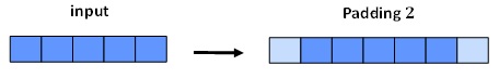
Fig. 1: Padding an array of length $5$ by $2$.

Stride: Given an array $x$ and a convolution kernel $h$, the convolution of $x$ and $h$ with stride $s$ is

$$(x*_{s}h)[i]=(x*h)[s\cdot i]$$

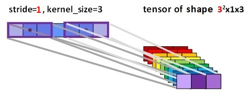
Fig. 2: 1D Tensor convolution with padding=3, stride=$4$ out_channels=$3$ on a length 5 array.

Pixel Shuffling: Let the pixelshuffle be $r$, given a tensor of shape $r\times N$ pixelshuffle [23] reshapes and rearranges it’s elements in a tensor of shape $rN$.

Fig. 3: Pixelshuffle of $3\times 1$ tensor returning a tensor of shape 3.

3.1 Fully Convolutional Fractional Scaling

The architecture we purpose, FCFS, carries out fractional scaling. Fully Convolutional Fractional Scaling: Given a real array $x$ and a scaling factor $\frac{r}{s}$, we define the following algorithm.

FCFS(input: Tensor) $\rightarrow$ Tensor:

x = pad(x, padding=$2K$)

x = conv(x, out_channels=$r$, stride=s,

kernel_shape=2K+1, kernel_weights=W)

return pixelshuffle(x, factors=$r$)

3.1.1 Description

The scaling is relative to the padded tensor of shape $N$. The architecture contains only a single hidden layer, whose shape is $r\times\frac{N}{s}$. Given a scale factor $\frac{r}{s}$ we apply a convolution with $stride=s$. Each of the $r$ convolution kernels produces an interpolation for offset $i+\frac{j-1}{r}\ \ s.t.\ j\in[1,..,r]$. Thus the hidden layer is of shape $r\times\frac{N}{s}$. Applying $pixelshuffle$ results in an array with the desired shape of $\frac{r}{s}N$

The parameters $K$, $kernel\_shape$, and $kernel\_weights$ depend on the interpolation method see examples section 5. The hidden layer’s shape is bilinearly dependent on output shape and $r$, which is the space and time complexity of the component.

4 2D & ND Extensions

The adaptations needed for 2D and ND are straightforward. Special attention needs to be paid to $Pixelshuffle$.

4.1 ND Pixelshuffle

Here we propose a slight generalization of Pixelshuffle.
PixelShuffle: For $n\geq 2$ and a tensor of shape $(r_{1}\cdot...\cdot r_{i}\cdot...\cdot r_{n})\times N_{1}\times...\times N_{i}\times...\times N_{n}$, Pixelshuffle rearranges the elements to a new tensor of shape $r_{1}N_{1}\times...\times r_{i}N_{i}\times...\times r_{n}N_{n}$

$$Out[i_{1},...,i_{i},...,i_{n}]=x[r,\lfloor\frac{i_{1}}{r_{1}}\rfloor,...,\lfloor\frac{i_{i}}{r_{i}}\rfloor,...,\lfloor\frac{i_{n}}{r_{n}}\rfloor]$$

$$r=\sum_{t=0}^{n-1}(\prod_{j=1}^{n-t-1}r_{j})((i_{n-t}-1)~{}{mod}~{}\ r_{n-t})$$

Figure 4 illustrates the formula.

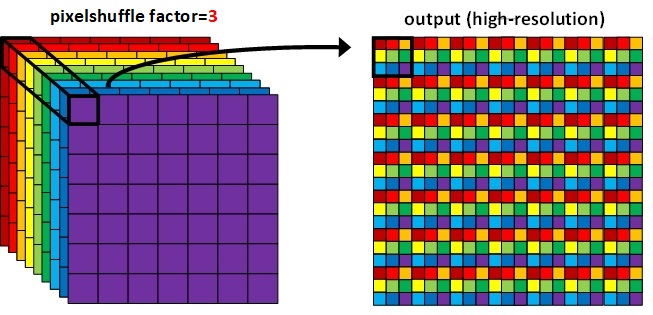
Fig. 4: Pixelshuffle of a $3^{2}\times 7\times 7$ tensor to a $3\cdot 7\times 3\cdot 7$ matrix.

4.2 ND Fully Convolutional Fractional Scaling

To scale an $ND$ input signal by scaling factors: $\frac{r_{1}}{s_{1}},...,\frac{r_{n}}{s_{n}}$ for the different dimensions.

FCFS(input: Tensor) $\rightarrow$ Tensor:

x = pad(x, padding=$2K_{1},\cdots,2K_{n})$

x = conv2d(x, out_channels=$\prod_{i}r_{i}$,

stride=[$s_{1},...,s_{n}$],

kernel_shape=[$2K_{1}+1,...,2K_{n}+1$],

kernel_weights=W

return pixelshuffle(x, factors=[$r_{1},...,r_{n}$])

5 EXAMPLES

5.1 Illustration of FCFS

Figure 5 illustrates FCFS on a $5\times 5$ image with a $\frac{3}{2}$ up-sacle factor. The output image is a $9\times 9$ image,

$$9\times 9=\frac{3}{2}\cdot(5+1)\times(5+1)\Longrightarrow\ output=\frac{3}{2}\cdot input$$

as expected.

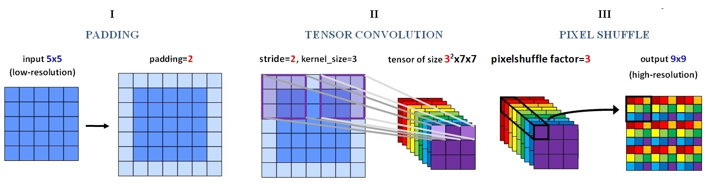
Fig. 5: Illustration of 2D $\frac{3}{2}$ Fully Convolutional Fractional Scaling.

5.2 Convolution’s kernel weights

$FCFS$ supports various scaling-methods through the parameters. In this section, we present kernel weights for various image scaling-methods.

Consider $f=\frac{3}{2}=\frac{r}{s}$ scaling. According to the offsets described in 3.1.1, we have $3^{2}=9(=r^{2})$ different kernels. We present the kernel of offsets $(1,1)$ and $(1,3)$ denoted by $W_{1,1}$ and $W_{1,3}$.

5.2.1 Nearest neighbour interpolation

From [24] nearest neighbour:

$$W_{1,1}:=\left[\begin{array}[]{cc}1.&0.0\\ 0.0&0.0\end{array}\right]~{}~{}W_{1,3}:=\left[\begin{array}[]{cc}0.0&1.0\\ 0.0&0.0\end{array}\right]$$

5.2.2 Bilinear interpolation

From [24], bilinear interpolation which is based on the 4 nearest pixels around the point of interpolation:

$$W_{1,1}:=\left[\begin{array}[]{cc}0.44&0.22\\ 0.22&0.11\end{array}\right]~{}~{}W_{1,3}:=\left[\begin{array}[]{cc}0.22&0.44\\ 0.11&0.22\end{array}\right]$$

5.2.3 Biqubic interpolation

From [24] bicubic interpolation as derived from the formula, published in [24]:

$${\displaystyle W(\Delta)={\begin{cases}1.5|\Delta|^{3}-2.5|\Delta|^{2}+1&{\text{for }}|\Delta|\leq 1,\\ -0.5|\Delta|^{3}+2.5|\Delta|^{2}-4|\Delta|-4a&{\text{for }}1<|\Delta|<2,\\ 0&{\text{otherwise}},\end{cases}}}$$

$\Delta=x-i,y-j$. Where the $x,y$ the subpixel point of interpolation and $i,j$ are the integer coordinates of the input image.

$$W_{1,1}:=\left[\begin{array}[]{ccc}0.16&0.16&0.07\\ 0.16&0.16&0.07\\ 0.07&0.07&0.03\end{array}\right]~{}~{}W_{1,3}:=\left[\begin{array}[]{ccc}0.13&0.13&0.13\\ 0.13&0.13&0.13\\ 0.05&0.05&0.05\end{array}\right]$$

6 Experiments

To test the time complexity and quality of FCFS we ran the following experiments:

1. We compared running times of FCFS to $torch.resize$ [25] for various scaling factors.

2. We computed two commonly used metrics, PSNR [26] and SSIM [26]. again comparing FCFS to $torch.resize$ [25], for various scaling factors.

6.1 Empirical methods

6.1.1 Scaling methods

Each experiment was repeated 100 times. We tested for the three different $scaling-methods$: ”nearest neighbours”, ”bilinear-interpolation” and ”bicubic-interpolation” The weights were implemented as described in section 5. For each method, six up-scaling factors and six down-scaling factors were tested

6.1.2 Hardware & Datasets

The experiments were carried out on NVIDIA RTX2070 GPU.

The dataset used was Celeb_A [27] with more than 200K celebrity images with 1024x1024 pixel resolution.

6.2 Results

6.2.1 Experiment results

The first experiment’s running time results are presented in figure 6. No significant difference was found between $torch.resize$ and $FCFS$, neither in up-scaling nor in down-scaling. The $FCFS$ was 0.0003 seconds slower on average.

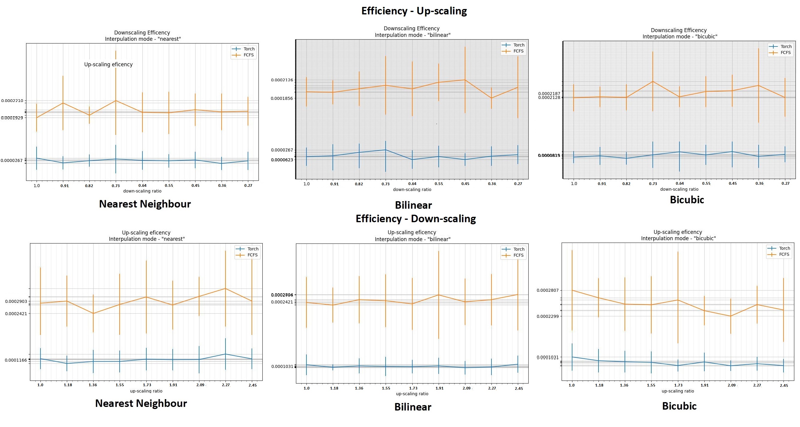
Fig. 6: Efficiency graphs for up/down-scaling tasks $\times$ different $scaling-methods$

The second experiment’s visual sameness results are presented in figures 7 and 8. Zooming in shows the visual artifacts that slightly differ between $FCFS$ and $torch.resize$.

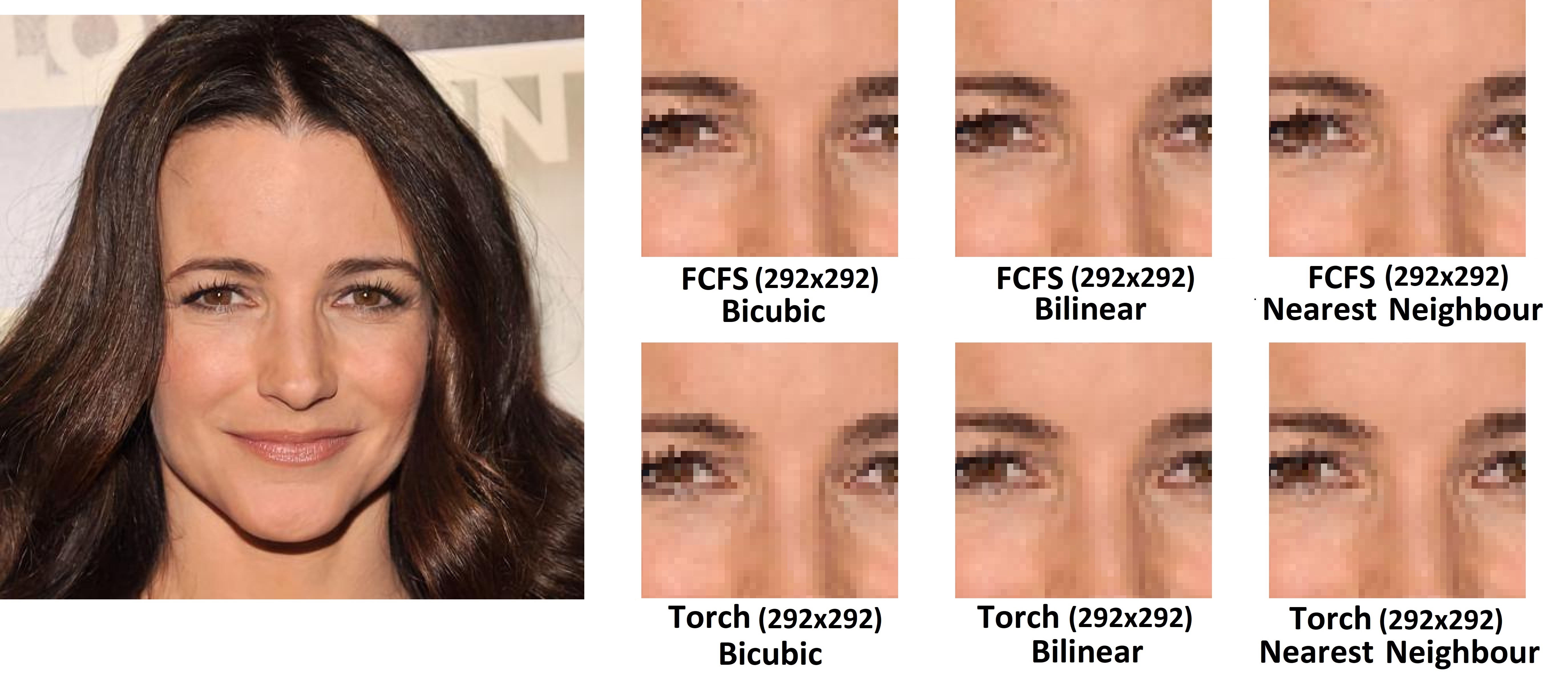
Fig. 7: Down-scaling by factor =$\frac{2}{11}$

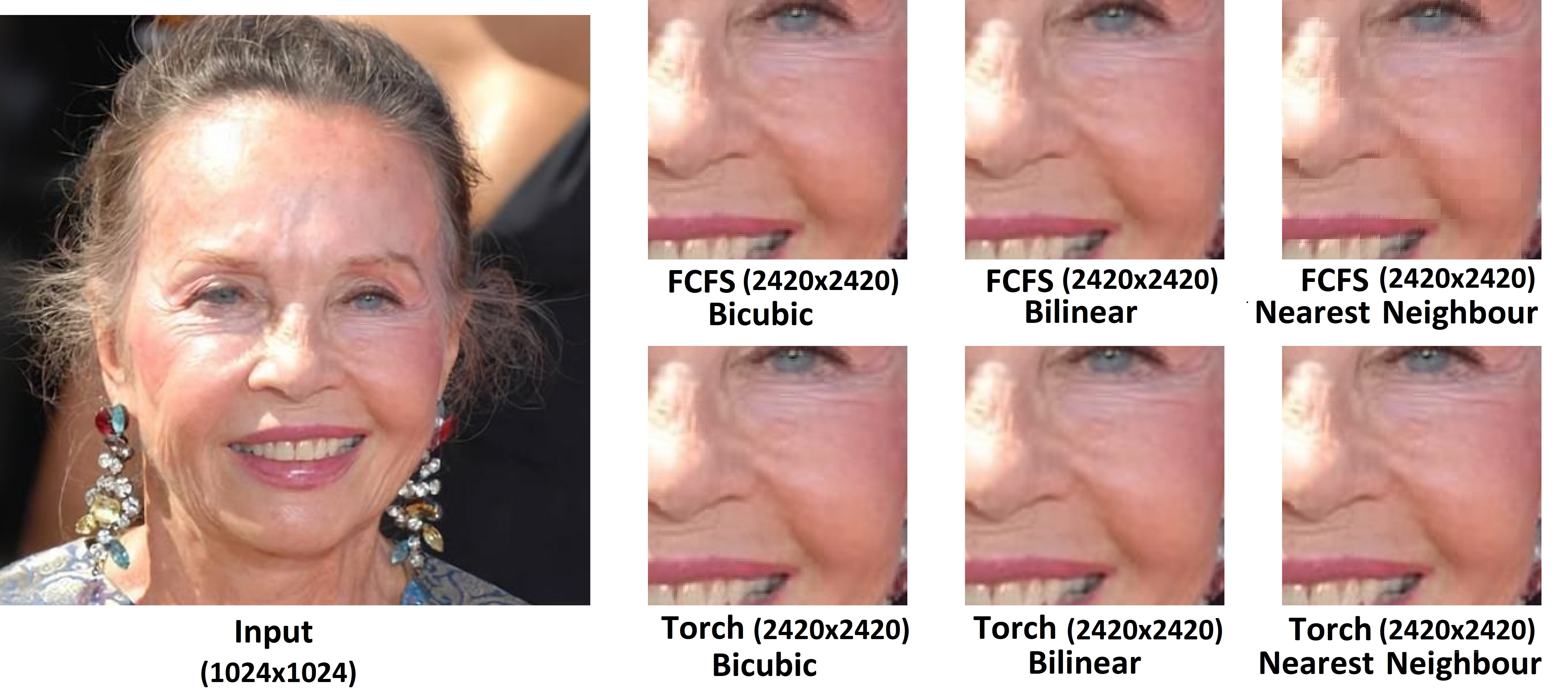
Fig. 8: Up-scaling by factor =$\frac{27}{11}$.

Figures 9 and 10 show distances between the output images for different $scaling-methods$. PSNR and SSIM values above $20$ and close to $1.00$ respectively support visual sameness [26]. The experiment shows the consistency of $FCFS$ with the $torch.resize$ implementation.

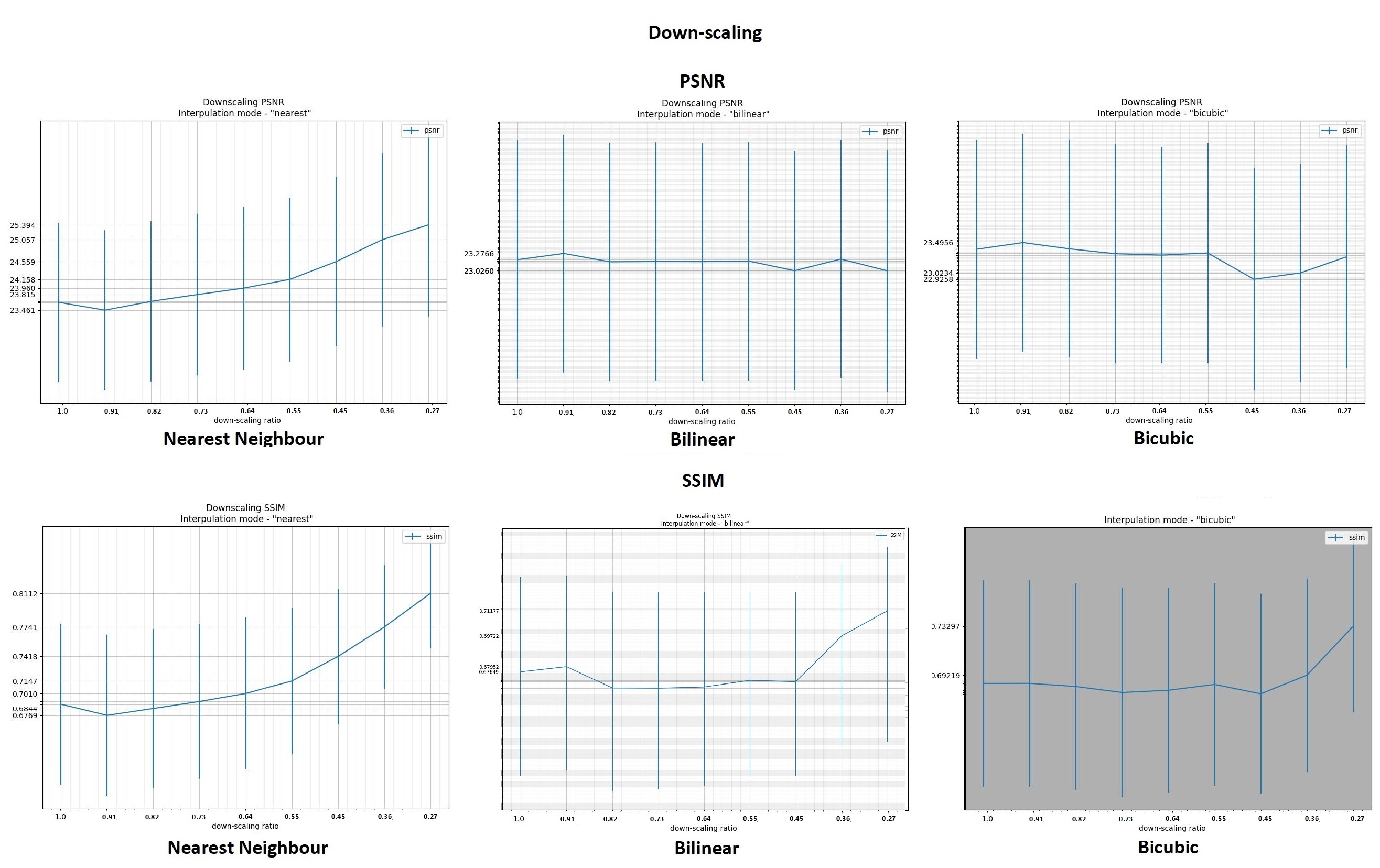
Fig. 9: PSNR & SSIM graphs for down-scaling tasks $\times$ different $scaling-methods$.

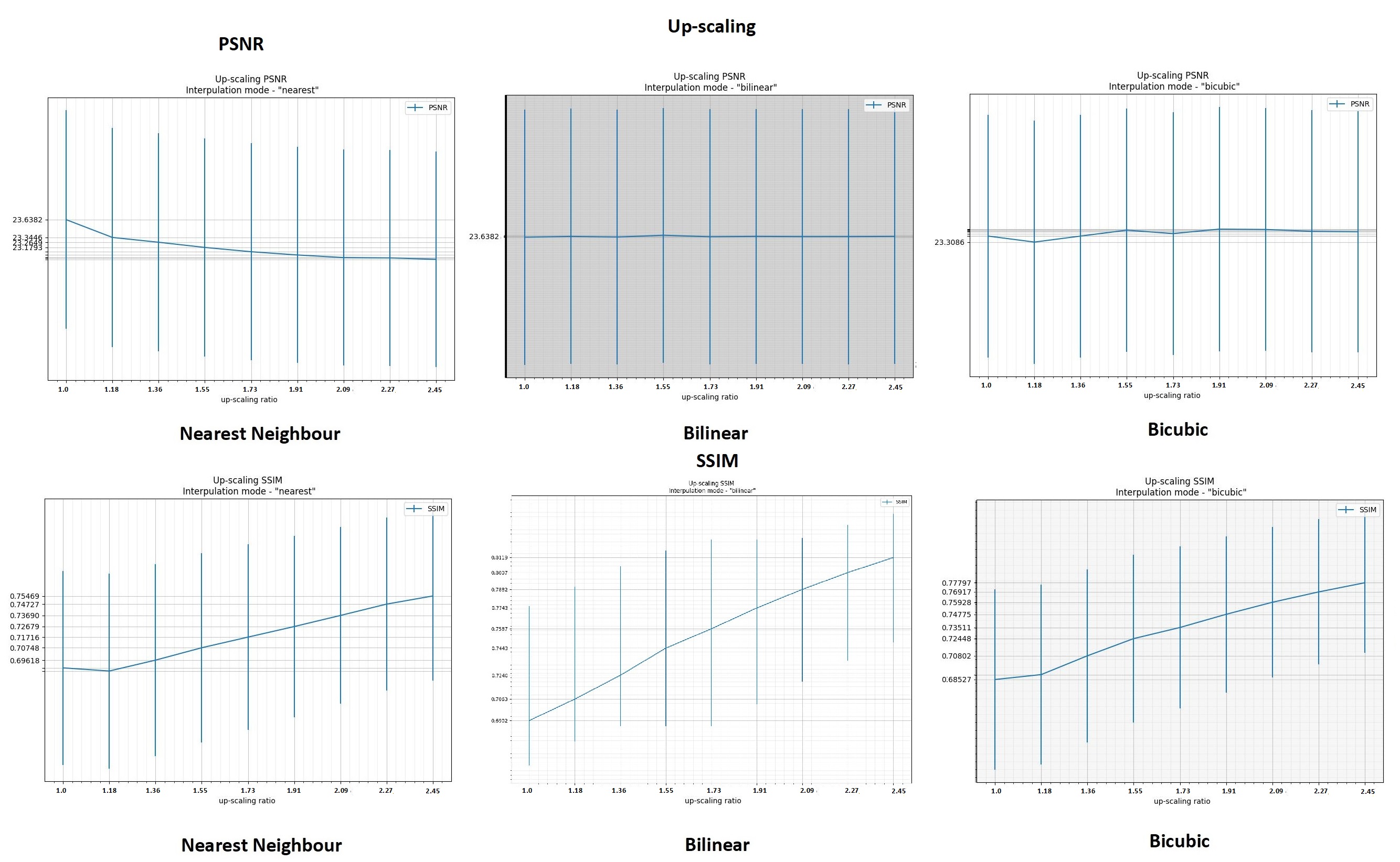
Fig. 10: PSNR & SSIM graphs for up-scaling tasks $\times$ different $scaling-methods$.

7 SUMMARY & FUTURE WORK

We introduced a fully convolutional fractional scaling component-$FCFS$ that is as efficient as the fixed shape scaling component ($torch.resize$).

The benefit from a convolution based approach is the ability to learn weights. FCFS allow to train the $kerenel\_weights$ and adjust them both in shape and values to the particular task. We aim to invest more effort in this direction in future work.

References

- [1] Jifeng Dai, Kaiming He, Yi Li, Shaoqing Ren, and Jian Sun, “Instance-sensitive fully convolutional networks,” in European Conference on Computer Vision. Springer, 2016, pp. 534–549.
- [2] Jonathan Long, Evan Shelhamer, and Trevor Darrell, “Fully convolutional networks for semantic segmentation,” in Proceedings of the IEEE conference on computer vision and pattern recognition, 2015, pp. 3431–3440.
- [3] Jun-Yan Zhu, Taesung Park, Phillip Isola, and Alexei A Efros, “Unpaired image-to-image translation using cycle-consistent adversarial networks,” in Proceedings of the IEEE international conference on computer vision, 2017, pp. 2223–2232.
- [4] Jin Yamanaka, Shigesumi Kuwashima, and Takio Kurita, “Fast and accurate image super resolution by deep cnn with skip connection and network in network,” in International Conference on Neural Information Processing. Springer, 2017, pp. 217–225.
- [5] S Yagnasree, A Subramanyam, and M Anand, “Image compression using neural networks,” NVEO-NATURAL VOLATILES & ESSENTIAL OILS Journal— NVEO, pp. 11088–11097, 2021.
- [6] Vivien Sainte Fare Garnot and Loic Landrieu, “Panoptic segmentation of satellite image time series with convolutional temporal attention networks,” in Proceedings of the IEEE/CVF International Conference on Computer Vision, 2021, pp. 4872–4881.
- [7] Wenguan Wang, Jianbing Shen, and Ling Shao, “Video salient object detection via fully convolutional networks,” IEEE Transactions on Image Processing, vol. 27, no. 1, pp. 38–49, 2017.
- [8] Yulun Zhang, Yapeng Tian, Yu Kong, Bineng Zhong, and Yun Fu, “Residual dense network for image restoration,” IEEE Transactions on Pattern Analysis and Machine Intelligence, vol. 43, no. 7, pp. 2480–2495, 2020.
- [9] Kunming Luo, Chuan Wang, Shuaicheng Liu, Haoqiang Fan, Jue Wang, and Jian Sun, “Upflow: Upsampling pyramid for unsupervised optical flow learning,” in Proceedings of the IEEE/CVF Conference on Computer Vision and Pattern Recognition (CVPR), June 2021, pp. 1045–1054.
- [10] Assaf Shocher, Nadav Cohen, and Michal Irani, “Zero-shot super-resolution using deep internal learning,” in Proceedings of the IEEE conference on computer vision and pattern recognition, 2018, pp. 3118–3126.
- [11] Jordi Pons, Santiago Pascual, Giulio Cengarle, and Joan Serrà, “Upsampling artifacts in neural audio synthesis,” in ICASSP 2021-2021 IEEE International Conference on Acoustics, Speech and Signal Processing (ICASSP). IEEE, 2021, pp. 3005–3009.
- [12] Anil Singh Parihar, Ritvik Mittal, Prashuk Jain, et al., “Video summarization using fully convolutional residual dense network,” in Sentimental Analysis and Deep Learning, pp. 47–58. Springer, 2022.
- [13] Shunta Maeda, “Unpaired image super-resolution using pseudo-supervision,” in Proceedings of the IEEE/CVF Conference on Computer Vision and Pattern Recognition, 2020, pp. 291–300.
- [14] Faraz Saeedan, Nicolas Weber, Michael Goesele, and Stefan Roth, “Detail-preserving pooling in deep networks,” in Proceedings of the IEEE Conference on Computer Vision and Pattern Recognition, 2018, pp. 9108–9116.
- [15] Juncheng Li, Faming Fang, Kangfu Mei, and Guixu Zhang, “Multi-scale residual network for image super-resolution,” in Proceedings of the European conference on computer vision (ECCV), 2018, pp. 517–532.
- [16] Yuan Yuan, Siyuan Liu, Jiawei Zhang, Yongbing Zhang, Chao Dong, and Liang Lin, “Unsupervised image super-resolution using cycle-in-cycle generative adversarial networks,” in Proceedings of the IEEE Conference on Computer Vision and Pattern Recognition Workshops, 2018, pp. 701–710.
- [17] Thomas Schlegl, Philipp Seeböck, Sebastian M Waldstein, Ursula Schmidt-Erfurth, and Georg Langs, “Unsupervised anomaly detection with generative adversarial networks to guide marker discovery,” in International conference on information processing in medical imaging. Springer, 2017, pp. 146–157.
- [18] Lynn Le, Luca Ambrogioni, Katja Seeliger, Yağmur Güçlütürk, Marcel van Gerven, and Umut Güçlü, “Brain2pix: Fully convolutional naturalistic video reconstruction from brain activity,” BioRxiv, 2021.
- [19] Benjamin Graham, “Fractional max-pooling,” arXiv preprint arXiv:1412.6071, 2014.
- [20] Shuangfei Zhai, Hui Wu, Abhishek Kumar, Yu Cheng, Yongxi Lu, Zhongfei Zhang, and Rogerio Feris, “S3pool: Pooling with stochastic spatial sampling,” in Proceedings of the IEEE Conference on Computer Vision and Pattern Recognition (CVPR), July 2017.
- [21] Siang Thye Hang and Masaki Aono, “Bi-linearly weighted fractional max pooling,” Multimedia Tools and Applications, vol. 76, no. 21, pp. 22095–22117, 2017.
- [22] Li-Heng Chen, Christos G Bampis, Zhi Li, Chao Chen, and Alan C Bovik, “Convolutional block design for learned fractional downsampling,” arXiv preprint arXiv:2105.09999, 2021.
- [23] Wenzhe Shi, Jose Caballero, Ferenc Huszár, Johannes Totz, Andrew P Aitken, Rob Bishop, Daniel Rueckert, and Zehan Wang, “Real-time single image and video super-resolution using an efficient sub-pixel convolutional neural network,” in Proceedings of the IEEE conference on computer vision and pattern recognition, 2016, pp. 1874–1883.
- [24] Anton Trusov and Elena Limonova, “The analysis of projective transformation algorithms for image recognition on mobile devices,” in Twelfth International Conference on Machine Vision (ICMV 2019). International Society for Optics and Photonics, 2020, vol. 11433, p. 114330Y.
- [25] Ronan Collobert, “Torch tutorial,” Institut Dalle Molle d’Intelligence Artificielle Perceptive Institute, vol. 2, 2002.
- [26] Alain Hore and Djemel Ziou, “Image quality metrics: Psnr vs. ssim,” in 2010 20th international conference on pattern recognition. IEEE, 2010, pp. 2366–2369.
- [27] Ziwei Liu, Ping Luo, Xiaogang Wang, and Xiaoou Tang, “Large-scale celebfaces attributes (celeba) dataset,” Retrieved August, vol. 15, no. 2018, pp. 11, 2018.