Shaking the causal tree: On the faithfulness and minimality assumptions beyond pairwise interactions

Abstract

Built upon the concept of causal faithfulness, the so-called causal discovery algorithms propose the breakdown of mutual information (MI) and conditional mutual information (CMI) into sets of variables to reveal causal influences. These algorithms suffer from the lack of accounting emergent causes when connecting links, resulting in a spuriously embellished view of the organization of complex systems. Here, we show that causal emergent information is necessarily contained in CMIs. We also connect this result with the intrinsic violation of faithfulness and elucidate the importance of the concept of causal minimality. Finally, we show how faithfulness can be wrongly assumed only because of the appearance of spurious correlations by providing an example of a non-pairwise system which should violate faithfulness, in principle, but it does not. The net result proposes an update to causal discovery algorithms, which can, in principle, detect and isolate emergent causal influences in the network reconstruction problems undetected so far.

Introduction.

Very large databases are a major opportunity for science, and data analytics is a remarkable growing field of investigation. A cornerstone inside this paradigm is the fact that the better one can characterize the causal model behind the data-generating complex system, the more one can understand how its mechanism works [1, 2]. Only with data on hands, an important task, then, is to correctly infer how the nodes inside the unknown system are generating its information dynamics and, consequently, determine the causation architecture behind the mechanisms.

In this scenario, causal discovery algorithms are powerful tools [3, 4] and they have been receiving substantial attention over the last decade thanks to the need to incorporate time-dependent data [5, 6, 7, 8, 9, 10, 11, 12]. A common thread in those works is to analyze the information transfer among processes at multiple spatio-temporal scales proposing a connection between causation and information theory. Indeed, causal analysis is performed on a set of interacting elements or state transitions, i.e., a causal model, and the hope is that information theory is the best way to quantify and formalize these interactions and transitions. To infer correct causal links from multivariate time-dependent data, the recent discovery algorithms use transfer-like quantifiers relying on concepts such as Granger causality and directed information theory [13, 14, 15], which are already formally justified by causal concepts such as $d$-separation and faithfulness [16, 17, 18].

The emerging field of non-pairwise network modeling [19, 20] is elucidating how standard networks embed pairwise relationships into our structural interpretation of the organization and behavior of complex systems giving a limited representation of higher-order interactions/synergism. In parallel to that, James et al. [21] pointed out how transfer-like analysis can be blinded to non-pairwise interactions. As elucidated in Ref.[10], but not taken forward, the point is that for synergic dependencies the concept of faithfulness can be violated by provoking the failure of all the algorithms above.

Since the appearance of causal models, considerable work has been done in the philosophy of causation into developing a general argument to use or to not faithfulness [4, 22, 23, 24, 25, 26]. A more pragmatic answer comes with the recent Weinberger proposal [27]. Instead of showing whether faithfulness fails or not, he argues that its use in a particular context may be defended by using general modeling assumptions rather than by relying on claims about how often it fails.

In this Letter, we make use of simple simulated systems, including higher-order interactions ones, to show quantitatively that genuine causal synergism violates faithfulness. We do so by claiming the importance of the conditioning operation in mutual information to capture pure synergism by formally connecting such concepts with partial information decomposition theory (PID) [28]. We connect this with the concept of causal minimality [3] elucidating its importance in determining tasks.

By comparing different structural organizations of non-pairwise systems, we also show exactly that causal faithfulness is recovered when specific types of redundancy are allowed in the PID eyes. Such a phenomenon manifests when the conditional mutual information (CMI) starts to fail, raising a trade-off between faithfulness and minimality. These results formally clarify a long-standing discussion about the regime of the faithfulness condition for causal discovery in non-pairwise scenarios.

Background.

In what follows, we denote random variables with capital letters, $X$, and their associated outcomes using lower case, $x\in\mathcal{X}$ with $\mathcal{X}$ the space of realizations. Random vectors, of size $n$, will be denoted by bold capital letters, $\mathbf{X}=\{X_{1},X_{2},\ldots,X_{n}\}$. For the sake of simplicity, in this text, we drop the time indices of temporal causal processes by assuming that the variables from $\mathbf{X}$ are in the past with respect to any univariate variable represented by the letter $Y$. In what follows we consider basic concepts from information theory and causality theory [3]. The amount of information the sources $\mathbf{X}$ (also called parents, $\text{PA}_{Y}$), carry about the target $Y$ is quantified by the mutual information (MI),

$$I(\mathbf{X};Y)=\sum_{\mathbf{x},y\in\mathcal{\mathbf{X}}\times\mathcal{Y}}p(\mathbf{X},Y)\log\>\frac{p(\mathbf{X},Y)}{p(\mathbf{X})p(Y)}.$$ (1)

A core limitation of MI when assessing systems with more than two variables is that it gives little insight into how information is distributed over sets of multiple interacting variables. Consider the classic case of two elements $X_{1}$ and $X_{2}$ that regulate a third variable $Y$ via the exclusive logical operation with equal probabilities $p(X_{1})=p(X_{2})=\nicefrac{{1}}{{2}}$ for all values of $X_{1}$ and $X_{2}$. Then $I(X_{1};Y)=I(X_{2};Y)=0$ even though both are connected to $Y$. Note that from the chain rule [29] it follows that $0<I(X_{1},X_{2};Y)=I(X_{2};Y)+I(X_{1};Y|X_{2})=I(X_{1};Y|X_{2})$. The point is that the full information is synergically contained in $I(X_{1};Y|X_{2})$ as explained in what follows.

The PID framework addresses the issue above by a formal method to decompose the contribution of all informational combinations that a set of multiple sources variables provides from a single target variable. The work of Williams & Beer [28] was to realize that such combinations of information are well structured into a lattice of antichains,

$$\normalsize\mathcal{A}(\mathbf{X})=\{\alpha\in\mathcal{P}^{+}(\mathcal{P}^{+}(\mathbf{X})):a_{1}\not\subset a_{2},\,\forall a_{1},a_{2}\in\alpha\},$$ (2)

where $\mathcal{P}^{+}(S)=\mathcal{P}(S)\setminus\{\emptyset\}$ denotes the set of nonempty subsets of $S$.

These possible combinations of information are called partial informational atoms (PI’s) and are defined by the mapping: $\alpha\mapsto I_{\partial}(\alpha;Y)$. Decomposing CMI and MI into PI’s and applying this to the XOR process discussed above, with $\mathbf{X}=\{X_{1},X_{2}\}$ and a single target variable $Y$ we have that,

$$I(X_{1};Y) = \text{Uni}(X_{1};Y)+\text{Red}(X_{1},X_{2};Y),$$ (3)

$$I(X_{2};Y) = \text{Uni}(X_{2};Y)+\text{Red}(X_{1},X_{2};Y),$$ (4)

$$I(X_{1};Y|X_{2}) = \text{Uni}(X_{1};Y)+\text{Syn}(X_{1},X_{2};Y),\vspace{-.4cm}$$ (5)

where $\text{Red}(X_{1},X_{2};Y)$ is the PI about $Y$ that is redundantly shared between $X_{1}$ and $X_{2}$, $\text{Uni}(X_{1};Y)$ refers to the PI about $Y$ that is uniquely present in $X_{1}$ and not in $X_{2}$, and $\text{Syn}(X_{1},X_{2};Y)$ is the PI about $Y$ that is only revealed by the joint states of $X_{1}$ and $X_{2}$ considered together. From Eq.5 we can see that the causal link from $\{X_{1},X_{2}\}$ to $Y$ is due to the synergic term $\text{Syn}(X_{1},X_{2};Y)$.

The existence of this link, even though $I(X_{i};Y)=0$, $i=1,2$, is known as a violation of the causal faithfulness condition. Note, however, that the concept of causal minimality is still satisfied since conditional independence plays a role here. Also, if $p(X_{1})\neq p(X_{2})$ in the example above, faithfulness is not violated anymore raising the common claim that its violations are rather pathological [9, 10, 12]. Below, we consider a simple causal process showing that when studying synergism, faithfulness violations are not rare corner cases, but can be prevalent in the space of probability distributions.

Example 1 (Failure of faithfulness).

Consider $\mathbf{X}=\{X_{1},X_{2},X_{3}\}$ as three independent binary sources and the target node $Y$ being the logical OR operation (symbol $\wedge$) between $X_{1}\oplus X_{2}$ ($\oplus$ means the exclusive or, XOR operation) and $X_{3}$, and the probability distribution table given by the table below with $0\leq f\leq 1$:

By computing the MIs and CMI $\times$ $f$, see Fig.1, we can see that $MI(X_{2};Y)=0$, but $CMI(X_{1};Y|X_{2},X_{3})\neq 0\;,\forall f>0$, showing a simple system where faithfulness is violated but minimality is not, in a non-pathological way.

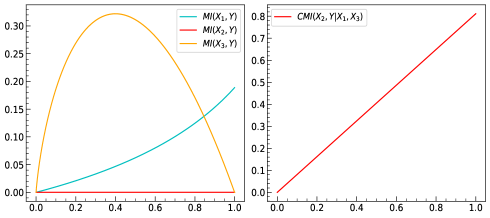
Figure 1: (left) $MI(X_{i})$ for $i=1,2,3$ and (right) $CMI(X_{1}|X_{2},X_{3})$ varying $0\leq f\leq 1$.

Discussion.

In the example 1 above, the robustness of minimality inside the context of the high-order interactions seems to be related to the need to consider conditioned independencies. This point motivates us to view more carefully the conditioning operation under the PID eyes. The natural question, therefore, raises: Is there a subset $\mathcal{S}(\mathbf{X})\subset\mathcal{A}(\mathbf{X})$, in which its elements form a lattice such that one can isolate only synergic nodes in $\mathcal{S}$?

To do so, we will look deeper into the PID approach in the search for $\mathcal{S}(\mathbf{X})$. To start, we propose Def.1 which gives a formal definition for $\mathcal{S}(\mathbf{X})$ allowing us to connect it with the conditioning operation, Prop.1 with proof in App.B.

Definition 1 (The redundant and synergic sets).

Given a set of sources $\mathbf{X}=\{X_{1},X_{2},\ldots,X_{n}\}$ we say that the subset $\mathcal{B}\subset\mathcal{A}(\mathbf{X})$, for $2\leq k\leq n$, is:

1. synergic of order $k$: This set is represented by the singletons inside $\mathcal{A}(\mathbf{X})$ with size $k$. In this case, we denote $\mathcal{B}\equiv\mathcal{S}^{(k)}(\mathbf{X})$;

2. redundant of order $k$: This set is represented by all elements $\beta$ inside $\mathcal{A}(\mathbf{X})$ of the form $\beta=\{\{b_{1}\},\{b_{2}\},\ldots\}$, s.t., exists $b_{j}\in\beta$, $|b_{j}|=k$. Then, $\mathcal{B}\equiv\mathcal{R}^{(k)}(\mathbf{X})$;

When considered all the orders $k$ we will omit the superscript, having then $\mathcal{S}(\mathbf{X})=\bigcup_{k}\mathcal{S}^{(k)}(\mathbf{X})$ and $\mathcal{R}(\mathbf{X})=\bigcup_{k}\mathcal{R}^{(k)}(\mathbf{X})$, respectively. Note that $\mathcal{A}(\mathbf{X})=\mathcal{R}(\mathbf{X})\sqcup\mathcal{S}(\mathbf{X})$. For a illustration of these sets, see Fig.B2.

Proposition 1 (Synergic property of the conditioning set).

Given a node $X_{j}\in\mathbf{X}$, with $\mathbf{X}=\{X_{1},X_{2},\ldots,X_{n}\}$ and $\mathbf{Z}\subseteq\mathbf{X}\setminus X_{j}$ with $|\mathbf{Z}|=k-2$, $2\leq k\leq n$. Then, $I(X_{j};Y\mid\mathbf{Z})$ includes all $\{\mathcal{S}^{(i)}(\mathbf{X})\}_{i=1}^{k}$. Furthermore, the term $\mathcal{S}^{(k)}$ increases monotonically according to $|\mathbf{Z}|$ on $\mathcal{A}(\mathbf{X})$.

To elucidate Prop.1 we consider a scenario where the non-pairwise relationships between $\mathbf{X}$ and $Y$ can be expressed as a Gibbs distribution. Full simulation details are reported in App.C. To start, we show the importance of the conditioned set size, $|\mathbf{Z}|$, to capture information contribution from non-pairwise terms. To do so, we consider a system of $n+1$ spins, with Hamiltonians having interactions only of order $k$,

$$H_{k}(\mathbf{X})=-\sum_{|\bm{\alpha}|=k}J_{\bm{\alpha}}\prod_{i\in\bm{\alpha}}X_{i}X_{n+1},$$ (6)

where $J_{\bm{\alpha}}$ are the interaction coefficients the and the sum runs over all collections of indices $\bm{\alpha}\subseteq[n]$ of cardinality $|\bm{\alpha}|=k$.

For these systems, we calculate the average normalized CMI, $\overline{CMI}$, to measure the strength of the high-order statistical effects beyond pairwise interactions (Fig.2). Our results confirm that to get information from a causal influence of order $k$ we have to account for conditioned sets of proportional size. Furthermore, the pairwise interaction regime is the only case where MIs (CMIs with $|\mathbf{Z}|=\emptyset$) are nonzero showing the violation of faithfulness for non-pairwise interactions.

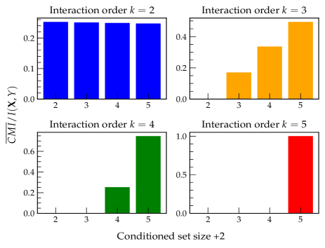
Figure 2: Growth of the $\overline{CMI}$ according to the conditioned set size. Here, we consider systems of size $n+1=5$ with interaction orders $k=2,3,4,5$ obeying Eq.(6) where the last node, $X_{5}$, was considered as a target. The calculation of the $\overline{CMI}$ was made over all permutations of the set $\{X_{i}\}_{i=1}^{4}$ in the CMI formula.

Note that, by viewing $\mathcal{A}(\mathbf{X})$ as a causal informational lattice, $\mathcal{A}(\text{PA}_{Y})$, where $\text{PA}_{Y}\equiv\mathbf{X}$ emphasizes that $\mathbf{X}$ is the set of parents of $Y$, and using the terminology of Def.(1) we can identify the concepts of faithfulness and minimality in the PID language, see Prop.(2) with proof in App.B1. This allow us to clarify why faithfulness fails and minimality is necessary to capture high-order causal dependencies.

Proposition 2 (Faithfulness & Minimality).

Let $\alpha\in\mathcal{A}(\text{PA}_{Y})$ be, then the causal influence of $\alpha$ in $Y$ satisfies,

1. faithfulness if $\alpha$, necessarily, belongs to $\mathcal{S}^{(2)}$, i.e., is independent of the others parents; and,

2. minimality/contextual-dependency if $\alpha$ belongs to $\mathcal{S}^{(k\geq 2)}$ $\forall k$, i.e., could depend on the others parents.

Prop.2-(a,b) straightly enlighten in an informational way how minimality includes faithfulness. The set $\mathcal{R}^{(2)}(\text{PA}_{Y})$ can be viewed as redundancy among only faithful causes. And, $\mathcal{R}^{(k\geq 2)}(\text{PA}_{Y})$ as redundancy among faithfully and contextually-dependent causes or only contextually-dependent causes.

The illusion of faithfulness or the deluge of redundancy?

Here, we analyze deeper why faithfulness can become optimal because of spurious correlations instead of genuine regularities. To answer this question, we fix the system size and investigate how a change in the organization of the interactions impacts the structure of the informational antichains and, consequently, the computation of MIs and CMIs. We will consider Hamiltonians with interactions up to order $k$,

$$H_{k}(\mathbf{X}) = -\sum_{i=1}^{n+1}J_{i}X_{i}-\sum_{i=1}^{n}\sum_{j=i+1}^{n+1}J_{ij}X_{i}X_{j}$$ (7)

$$- \ldots-\sum_{|\bm{\alpha}|=k}J_{\bm{\alpha}}\prod_{i\in\bm{\alpha}}X_{i},\vspace{-.3cm}$$

Firstly, we model non-pairwise components exclusively in the Hamiltonian, which means that if a node has the interaction of order $k$, it cannot interact anymore, represented by the causal directed hyper-graph in Fig.(3-A). For the second case, we relax the exclusivity condition, represented graphically by a dense cloud of connectivity, Fig.(3-B).

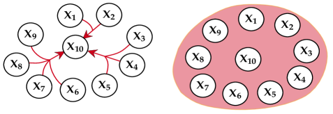
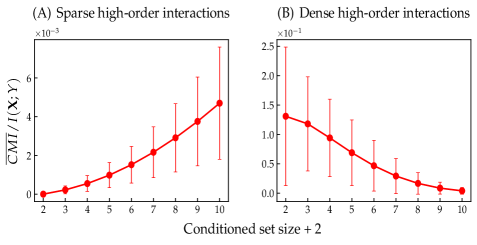
Figure 3: Here, we simulate two non-pairwise systems of size $n+1=11$ following Eq.(7) with different organization. (A) This model has spins with only exclusive interactions of order $k=3,4,5$. (B) Here we are allowing all possible interactions of order $k=3,\ldots,10$. Again the last spin, $X_{n+1}$, was considered as target node $Y$, and the calculation of $\overline{CMI}$ was done as explained in the previous figure.

Our results show that when the Hamiltonian only possesses exclusive non-pairwise interactions, faithfulness still fails in capturing causal influence. Also, the monotonic increase of the $CMI$ according to the conditioning set size is preserved showing how minimality remains robust to identify high-order of synergism, Fig.3-(A). However, when we relax the exclusivity condition, even without pairwise interactions, the MI’s are nonzero anymore. More intriguing, faithfulness beats minimality and the latter does not seem to be optimal in capturing synergism anymore, Fig.3-(B).

We argue that such behavior is due to the appearance of a specific type of redundancy, induced by the functional properties of the system. Indeed, as generated independently, we would expected that $MI(X_{i},X_{j})=0$ for any sources $X_{i},X_{j}\in\text{PA}_{Y}$, which is the case for the system of Fig.3-(A). However, it occurs that in the system of Fig.3-(B), we have $MI(X_{i},X_{j})\neq 0$. The existence of these correlations among the sources spuriously inflates the calculation of MIs while it provokes the decrease of CMIs according to the conditioning set size.

Such redundancy is similar to the concept of mechanistic nature [30, 31]. In its simplest form, this type of redundancy occurs when the sources are generated independently and are related to the functional properties of the system as well. While its importance has been recognized, how to define or quantify this type of redundancy inside PID is an open question [32]. In our case, it is due to the existence of correlations between atoms not explored in the informational antichain, e.g., $\{\{X_{1}\}\}$ and $\{\{X_{1}X_{2}\}\}$.

This elucidation also allows us to explain the balance between MIs and CMIs in the multivariate case. Indeed, it is well-known that for the case of three random variables $X,Y$, and $Z$, the following interpretation holds [33]:

$$I(X;Y) < I(X;Y|Z)\Longrightarrow\text{synergism}$$ (8)

$$I(X;Y) > I(X;Y|Z)\Longrightarrow\text{redundancy}$$ (9)

By the above argumentation we have found empirically that, for high-order systems, $\mathbf{Z}_{1}\subset\mathbf{Z}_{2}\subseteq\text{PA}_{Y}$,

$$I(X;Y|\mathbf{Z}_{1}) < I(X;Y|\mathbf{Z}_{2})\Longrightarrow\text{synergism}$$ (10)

$$I(X;Y|\mathbf{Z}_{1}) > I(X;Y|\mathbf{Z}_{2})\Longrightarrow\text{redundancy}$$ (11)

where the first inequality holds when the exclusivity condition is satisfied, $\mathcal{R}(\mathbf{X})\equiv\mathcal{R}_{E}(\mathbf{X})$, meaning no redundancy dominance; and, the second inequality becomes true according to the growth of the system and mechanistic redundancy dominance.

Conclusions and Consequences.

The XOR problem is a classical problem in the domain of AI which was one of the reasons for the AI winter during the 70s in the neural networks context [34]. Here, we showed how the difficulties with concepts of statistical independence for the XOR operation raise a problem in the causal discovery domain, as well as when dealing with non-pairwise/synergic relationships. By doing so, we raised the importance of incorporating concepts, namely, partial information theory, beyond the classical Shannon approach when dealing with the concept of synergism. This strengthens the already well-established link between causality and information theory.

Specifically, we have elucidated a new way to interpret the concepts of faithfulness and minimality from the causality domain clarifying the failure and importance of these conditions for network discovery beyond pairwise interaction. We showed that, while well accepted, faithfulness fails to capture synergism when the latter is properly defined. And, its assumption is more related to the appearance of spurious regularities than genuine causal influences.

Indeed we argued that this specific spuriousness can be linked with the concept of (mechanistic) redundancy [30]. While important in view of formalizing the founded empirical inequalities in Eq.10, a qualitative approach is missing in the literature and we leave it for future work. This would be important for a better understating of some phenomena from multivariate information theory.

A possible path in this domain could be to incorporate the so-called context-specific independence (CSI) [35], which is the independence that holds in a certain value of conditioned variables, i.e., the context.

It has been shown that the presence and knowledge of such independence lead to more efficient probabilistic inference by exploiting the local structure of the causal models [36]. The XOR operation follows such relations [37]. Also, it allows the identification of causal effects, which would not be possible without any information about CSI relationships [38]. Further investigations of this approach in synergic causal discovery from large data sets we leave for future work.

Also, our separation of the informational antichain in the subsets $\mathcal{R(\mathbf{X})}$ and $\mathcal{S(\mathbf{X})}$, called strong synergism condition [39], has not been incorporated in the field of causal synergism/emergence [40, 41, 42]. It would be interesting to compare these approaches aiming at a different quantifier for causal emergence influences.

Acknowledgments

The authors would like to thanks prof. D. Mašulović for fruitful discussion. Also, to P. Mediano by provide the codes which helped the simulations, T. Perón and K. Roster for reading the manuscript. The project was funded by Brazilian funding agencies CNPq (Grant No.140665/2018-8) and FAPESP (Grant No.2018/12072-0).

Supplementary Material

Appendix A Causal Models

Definition A1 (Causal Models).

A causal model $\mathcal{M}$ is a 2-tuple $\braket{G_{u},P_{u}}$, where $G_{u}=(X,E)$ is directed acyclic graph (DAG) with edges $E$ that indicate the causal connections among a set of nodes $X$ and a given set of background conditions (state of exogenous variables) $U=u$. The nodes in $G_{u}$ represent a set of associated random variables, denoted by $X$ with probability function

$$P(x_{i}|\mathrm{pa}_{i})=\sum_{u_{i}}P(x_{i}|\mathrm{pa}_{i},u_{i})P(u_{i}).$$ (A1)

where $\mathrm{pa}_{i}$ defines the parents for any node $X_{i}\in X$ (all nodes with an edge leading into $X_{i}$).

For a causal graph, there is the additional requirement that the edges $E$ capture causal dependencies (instead of only correlations) between nodes. This means that the decomposition $P(x)=\prod_{i}P(x_{i}|\mathrm{pa}_{i})$ holds, even if the parent variables are actively set into their state as opposed to passively observed in that state (causal Markov condition (CMC) [43, 3]),

$$P(x_{i}|\mathrm{pa}_{i})=\prod_{i}P(x_{i}|\mathrm{pa}_{i})=\prod_{i}P(x_{i}|\mathrm{do}(\mathrm{pa}_{i}))$$ (A2)

Definition A2 (Spatio-temporal Causal Models).

A spatio-temporal causal model $\mathcal{M}_{t}$ defines a partition of its nodes $X$ into $k+1$ temporally ordered steps, $X=\{X_{0},X_{1},\ldots,X_{k}\}$, where $(\mathrm{pa}(X_{0})=\emptyset)$ and such that the parents of each successive step are fully contained within the previous step $(\mathrm{pa}(X_{t})\subseteq X_{t-1},t=1,\ldots,k)$ [44]. This definition avoids “instantaneous causation” between variables, which means that $\mathcal{M}_{t}$ fulfills the temporal Markov property [17]. We also assume that $U$ contains all relevant background variables, any statistical dependencies between $X_{t-1}$ and $X_{t}$ are causal dependencies, and cannot be explained by latent external variables (causal sufficiency condition [10]).

Finally, because time is explicit in $G_{u}$ and we assume that there is no instantaneous causation, then the earlier variables, $X_{t-1}$, influence the later variables, $X_{t}$. And, remembering that the background variables $U$ are conditioned to a particular state $u$ throughout the causal analysis they are, otherwise, not further considered. Together, these assumptions imply a transition probability function for $X$ [44],

$$P_{u}(x_{t}|x_{t-1})=\prod_{i}P_{u}(x_{i}|x_{t-1})=\prod_{i}P_{u}(x_{i}|\mathrm{do}(x_{t-1})),$$ (A3)

i.e., nodes at time $t$ are conditionally independent given the state of the nodes at time $t-1$.

The part $X=\{X_{0},X_{1},\ldots,X_{k}\}$ in a spatio-temporal causal model can be interpreted as consecutive time steps of a discrete dynamical system of interacting elements; a particular state $X=x$, then, corresponds to a system transient over $k+1$ time steps, e.g. the directed Ising model used in the main text. As already mentioned in the main text, to not get confused with the subindices meaning time steps or different processes we denoted variables in the past by $X$ and in the present by $Y$.

A1 Faithfulness and Minimality

So far, we discussed the assumptions in causal models, which enables us to read off statistical independencies from the graph structure. As our goal here is causal discovery, we need to consider concepts with allows us to infer dependencies from the graph structure such as Faithfulness and Minimality.

Definition A3 (Faithfulness & Minimality).

Consider the causal model $\mathcal{M}=\{P,G\}$, the target $Y$ and its parent set $\text{PA}_{Y}=\{X_{1},X_{2},\ldots,X_{n}\}$. Assume that the joint distribution has a density $P$ with respect to a product measure. Then,
(F) $P$ is faithful with respect to the DAG $G$ if $(X_{K}\rotatebox[origin={c}]{90.0}{$\models$}_{P}Y|X_{L})$ whenever $(K\cap\text{PA}_{Y})\neq(L\cap\text{PA}_{Y})$ $\forall K,L\subset G$;
(M) $P$ satisfies causal minimality with respect to $G$ if and only if $\forall Y$, we have that $X_{i}\centernot{\rotatebox[origin={c}]{90.0}{$\models$}}Y|(\text{PA}_{Y}\setminus X_{i})$, $\forall X_{i}\in\text{PA}_{Y}$.

Condition (F) ensures that the set of causal parents is unique and that every causal parent presents an observable effect regardless of the information about other causal parents [9, 3]. On the other hand, (M) says that a distribution is minimal with respect to a causal graph if and only if there is no node that is conditionally independent of any of its parents, given the remaining parents. In some sense, all the parents are “active” [18]. Suppose now, we are given a causal model, for example, in which causal minimality is violated. Then, one of the edges is “inactive”. This is in conflict with the definition of (F), then

Proposition A1 (Faithfulness implies causal minimality).

If $P$ is faithful and Markovian with respect to $G$, then causal minimality is satisfied.

Appendix B Informational lattices

According to Williaws & Beer [28], to capture all different kinds of partial information contribution in the MI one should split the domain in such way which different elements do not share common information among them. In other words, the domain of this set can be reduced to the collection of all sets of sources such that no source is a superset of any other, formally

Definition B4 (The informational antichain).

Consider the ensemble of variables $\mathbf{X}=\{X_{1},X_{2},\ldots,X_{n}\}$, which are informational sources to the target $Y$. The set

$$\begin{gathered}\mathcal{A}(\mathbf{X})=\{\alpha\in\mathcal{P}^{+}(\mathcal{P}^{+}(\mathbf{X})):a_{1}\not\subset a_{2},\,\forall a_{1},a_{2}\in\alpha\},\end{gathered}$$ (B4)

where $\mathcal{P}^{+}(S)=\mathcal{P}(S)\setminus\{\emptyset\}$ denotes the set of nonempty subsets of $S$, is called the informational antichain of the sources $\mathbf{X}$. Henceforth, we will denote sets of $\mathcal{A}(\mathbf{X})$, corresponding to collections of sources, omitting the brackets with a dot separating the sets within an antichain, and the groups of sources are represented by their variables with respective indices concatenated. For example, $X_{1}\cdot X_{2}X_{3}$ represents the antichain $\{\{X_{1}\}\{X_{2},X_{3}\}\}$ [21].

Antichains form a lattice [45], having a natural hierarchical structure of partial order over the elements of $\mathcal{A}(\mathbf{X})$,

$$\forall\alpha,\beta\in\mathcal{A}(\mathbf{X}),\;\alpha\preceq\beta\iff(\forall b\in\beta:\;\exists a\in\alpha,\;a\subseteq b).$$ (B5)

When ascending the lattice, the redundancy function $I_{\cap}(\alpha,Y)$, monotonically increases, being a cumulative measure of information where higher element provides at least as much information as a lower one [28]. The inverse of $I_{\cap}(\alpha,Y)$ called the partial information functions (PI-functions) and denoted by $I_{\partial}$ measures the partial information contributed uniquely by each particular element of $\mathcal{A}(\mathbf{X})$. This partial information will form the atoms into which we decompose the total information that $\mathbf{X}$ provides about $Y$. For a collection of sources $\alpha\in\mathcal{A}(\mathbf{X})$, the PI-functions are defined implicitly by

$$I_{\partial}(\alpha;Y)=I_{\cap}(\alpha;Y)-\sum_{\beta\prec\alpha}I_{\partial}(\beta;Y).$$ (B6)

Formally, $I_{\partial}$ corresponds to the the Möbius inverse of $I_{\cap}$. For singletons we have the identification $MI\equiv I_{\cap}$ such condition, called self-redundancy, allows the computation of the PI’s. The number of PI-atoms is the same as the cardinality of $\mathcal{A}(\mathbf{X})$ for $\mathbf{X}=n-1$ given by the $(n-1)$-th Dedekind number [45], which for $n=2,3,4,\ldots$ is $1,4,18,166,7579,\ldots$ which is super-exponential according to $|\mathbf{X}|$.

B1 Conditioning antichains

Going to the PID in the multivariate case is not so straight. Indeed, adding only one variable more it is sufficient to see the failure of elimination of redundancy when conditioning. Consider the three variable case, $\mathbf{X}=\{X_{1},X_{2},X_{3}\}$, then

$$I(X_{1};Y|X_{2},X_{3}) = I(X_{1},X_{2},X_{3};Y)-I(X_{2},X_{3};Y)$$

$$= I_{\partial}(X_{1};Y)+I_{\partial}(X_{1}X_{2};Y)+I_{\partial}(X_{1}X_{3};Y)+I_{\partial}(X_{1}X_{2}\cdot X_{1}X_{3};Y).$$

From Eq.B1, we can see that there is existence of redundancy in the last term which is not eliminated by the operation of conditioning, see Fig.B2. This is because there are new kinds of terms representing combinations of redundancy and synergy which are not include in the down set of $\{X_{2},X_{3}\}$, $\mathord{\downarrow}\{X_{2},X_{3}\}$. On the other hand, we can see that all orders of synergic atoms are included. Result below formalizes it.

Proposition B2 (PID view of conditioning operation).

Suppose that we have the set $\mathbf{X}=\{X_{1},X_{2},\ldots,X_{n}\}$ and $\mathbf{Z}\subseteq\mathbf{X}\setminus X$, with $X\in\mathbf{X}$. Then, the operation of conditioning on $\mathbf{Z}$ the information between $X$ and $Y$ is given by

$$I(X;Y\mid\mathbf{Z}) := I(X,\mathbf{Z};Y)-I(\mathbf{Z};Y)$$ (B8)

$$= \sum_{\alpha\in\downarrow\{X,\mathbf{Z}\}}I_{\partial}(\alpha;Y)-\sum_{\alpha\in\downarrow\mathbf{Z}}I_{\partial}(\alpha;Y)=\sum_{\alpha\in(\downarrow\mathbf{Z})^{\complement}}I_{\partial}(\alpha;Y)$$

where $(\mathord{\downarrow}\mathbf{Z})^{\complement}$ is the complementary set of $\mathord{\downarrow}\mathbf{Z}$ given the particular subset of collections of $\mathbf{X}$ used to build the information lattice, in this case, was $\{X,\mathbf{Z}\}$.

Proof of Prop.1.

Lets show the synergism monotonic increasing. This can be seen by noting that the cardinality of $\mathbf{Z}$ — which means conditioning on higher nodes of the lattice — tells the order of synergic terms that $I(X_{j};Y\mid\mathbf{Z})$ includes. Indeed, suppose that we want to include all synergic influence of orders $\leq n$ among $X_{j}\in\mathbf{X}$ and $n-1$ elements from $\mathbf{X}\setminus X_{j}$ on node $Y$. Then, w.l.o.g., consider $\mathbf{Z}:=\mathbf{X}\setminus\{X_{1},X_{j}\}$ with $j\neq 1$, the expression

$$I(X_{j};Y\mid\mathbf{Z})=\sum_{\alpha\in(\downarrow\mathbf{Z})^{\complement}}I_{\partial}(\alpha;Y)$$ (B9)

does not include any synergic influence terms of order $n$ of the type $I_{\partial}(X_{1}..X_{j}..X_{n-1};Y)$. The argument is the same for $\mathbf{Z}:=\mathbf{X}\setminus\{X_{i},X_{j}\},\;1\leq i\neq j\leq n$. ∎

Proof of Prop.2.

Consider the joint distribution $P$ given by the tuple $(Y,PA_{Y})$ and the causal influence of $\alpha\in\mathcal{A}(PA_{Y})$. As $\alpha\in PA_{Y}$, then $\alpha$ is a singleton in $\mathcal{A}(PA_{Y})$ belonging to $\mathcal{S}^{(k\geq 2)}$.

1. Suppose that $\alpha$ is faithful. By using the correspondence $I(X;Y|Z)=0\Longleftrightarrow(X\rotatebox[origin={c}]{90.0}{$\models$}_{P}Y|Z)$ we can notice that $I(\alpha;Y)\neq 0$, by using $K\equiv\alpha$ and $L\equiv\emptyset$ in Def.6-(F). Using Prop.B2 for $Z\equiv\emptyset$ we have $\alpha\in\mathcal{S}^{(2)}$;

2. Now, suppose that $\alpha$ is minimal. Then $I(\alpha;Y|PA_{Y}\setminus\alpha)\neq 0$ by Def.6-(M) and, using Prop.B2 $\forall Z$ with $|Z|=k-2$ we have that $\alpha\in\mathcal{S}^{(k\geq 2)}$.

∎

B2 Graphical illustration of Def.1 in informational antichains

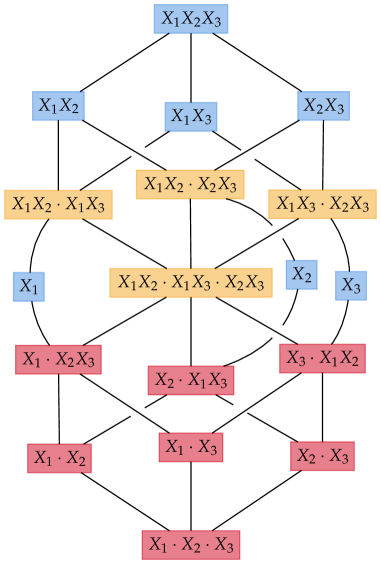
Figure B1: Illustration of Def.1 for the informational lattice $\mathcal{A}(\mathbf{X})$ with $\mathbf{X}=\{X_{1},X_{2},X_{3}\}$. Coloured boxes explanation:   atoms inside $\mathcal{S}^{(3)}(\mathbf{X})$;   +  atoms inside $\mathcal{R}^{(3)}(\mathbf{X})$;   atoms inside $\mathcal{R}^{(3)}_{E}(\mathbf{X})$.

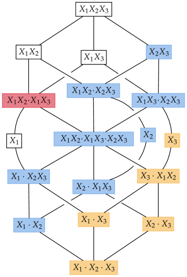
Figure B2: Illustration of the effect of conditioning the information between $\mathbf{X}=\{X_{1},X_{2},X_{3}\}$ and target node $Y$ on the element $\{X_{2}X_{3}\}\in\mathbf{X}^{-}$ against $\{X_{3}\}\in$ for informational lattice $\mathcal{A}(\mathbf{X})$. Coloured boxes explanation:   goes away when $X_{1}\mid\{X_{3}\}$;   +  goes away when $X_{1}\mid\{X_{2},X_{3}\}$;   remains only when $X_{1}\mid\{X_{2},X_{3}\}$.

Appendix C Simulation details

For all Figs.2, 3 the systems were of $n+1$ spins, where $\mathcal{X}_{i}=\{-1,1\}$ for $i=1,\ldots,n+1$ whose joint probability distributions can be expressed in the form $p_{\mathbf{X}_{n+1}}(\mathbf{x}_{n+1})=\exp\{H_{k}(\mathbf{X}_{n+1})\}/Z$, with $\beta$ the inverse temperature choose as $1$, $Z$ the normalisation constant to make sure that the $p_{\mathbf{X}_{n+1}}$’s are probabilities, and $H_{k}(\mathbf{X}_{n+1})$ the Hamiltonian function. In all simulations, all interaction coefficients $J$ in the Hamiltonians were generated i.i.d. from a uniform distribution weighted by the coefficient $0.2$. Also, $100$ Hamiltonians were sampled at random for each order $k$ in every experiment.

References

- Craver and Tabery [2019] C. Craver and J. Tabery, in The Stanford Encyclopedia of Philosophy, edited by E. N. Zalta (Metaphysics Research Lab, Stanford University, 2019) Summer 2019 ed.
- Hitchcock [2020] C. Hitchcock, in The Stanford Encyclopedia of Philosophy, edited by E. N. Zalta (Metaphysics Research Lab, Stanford University, 2020) Summer 2020 ed.
- Pearl [2009] J. Pearl, Causality: Models, Reasoning and Inference (Cambridge University Press, 2009).
- Spirtes et al. [2000] P. Spirtes, C. Glymour, and R. Scheines, Causation, Prediction, and Search, 2nd ed. (MIT press, 2000).
- Lizier and Rubinov [2013] J. T. Lizier and M. Rubinov, BMC Neuroscience 10.1186/1471-2202-14-S1-P337 (2013).
- Runge et al. [2012] J. Runge, J. Heitzig, V. Petoukhov, and J. Kurths, Phys. Rev. Lett. 108, 258701 (2012).
- Runge [2014] J. Runge, Detecting and quantifying causality from time series of complex systems, Ph.D. thesis, Humboldt-Universität zu Berlin, Mathematisch-Naturwissenschaftliche Fakultät (2014).
- Chicharro and Panzeri [2014] D. Chicharro and S. Panzeri, Frontiers in Neuroinformatics 8, 64 (2014).
- Sun et al. [2015] J. Sun, D. Taylor, and E. Bollt, SIAM Journal on Applied Dynamical Systems 14, 73 (2015), https://doi.org/10.1137/140956166 .
- Runge [2018] J. Runge, Chaos: An Interdisciplinary Journal of Nonlinear Science 28, 075310 (2018).
- Hlinka and Kořenek [2018] J. Hlinka and J. Kořenek, arXiv e-prints (2018), 1804.08173 .
- Novelli et al. [2019] L. Novelli, P. Wollstadt, P. Mediano, M. Wibral, and J. T. Lizier, Network Neuroscience 3, 827 (2019).
- Granger [1980] C. Granger, Journal of Economic Dynamics and Control 2, 329 (1980).
- Massey [1990] J. L. Massey, Causality, feedback and directed information (1990).
- Schreiber [2000] T. Schreiber, Phys. Rev. Lett. 85, 461 (2000).
- Eichler [2012] M. Eichler, Probability Theory and Related Fields 153, 233 (2012).
- Eichler [2013] M. Eichler, Philosophical Transactions of the Royal Society A: Mathematical, Physical and Engineering Sciences 371, 20110613 (2013).
- Peters et al. [2017] J. Peters, D. Janzing, and B. Schölkopf, Elements of Causal Inference - Foundations and Learning Algorithms, Adaptive Computation and Machine Learning Series (The MIT Press, Cambridge, MA, USA, 2017).
- Battiston et al. [2020] F. Battiston, G. Cencetti, I. Iacopini, V. Latora, M. Lucas, A. Patania, J.-G. Young, and G. Petri, Physics Reports 874, 1 (2020).
- Battiston et al. [2021] F. Battiston, E. Amico, A. Barrat, G. Bianconi, G. Ferraz de Arruda, B. Franceschiello, I. Iacopini, S. Kéfi, V. Latora, Y. Moreno, and et al., Nature Physics 17, 1093–1098 (2021).
- James et al. [2016] R. G. James, N. Barnett, and J. P. Crutchfield, Phys. Rev. Lett. 116, 238701 (2016).
- Cartwright [1999] N. Cartwright, The Dappled World: A Study of the Boundaries of Science (Cambridge University Press, 1999).
- Hoover [2001] K. D. Hoover, Causality in macroeconomics, in The Methodology of Empirical Macroeconomics (Cambridge University Press, 2001) p. 89–134.
- Steel [2006] D. Steel, Minds Mach. 16, 303 (2006).
- Andersen [2013] H. Andersen, Philosophy of Science 80, 672 (2013).
- Uhler et al. [2013] C. Uhler, G. Raskutti, P. Bühlmann, and B. Yu, The Annals of Statistics 41, 436 (2013).
- Weinberger [2018] N. Weinberger, Erkenntnis 83, 113 (2018).
- Williams and Beer [2010] P. L. Williams and R. D. Beer, CoRR abs/1004.2515 (2010).
- Cover and Thomas [2006] T. M. Cover and J. A. Thomas, Elements of Information Theory (Wiley Series in Telecommunications and Signal Processing) (Wiley-Interscience, New York, NY, USA, 2006).
- Harder et al. [2013] M. Harder, C. Salge, and D. Polani, Phys. Rev. E 87, 012130 (2013).
- James et al. [2018] R. G. James, J. Emenheiser, and J. P. Crutchfield, arXiv e-prints (2018).
- Ince [2017] R. A. A. Ince, Entropy 19, 10.3390/e19070318 (2017).
- Yeung [2008] R. W. Yeung, Information Theory and Network Coding, 1st ed. (Springer Publishing Company, Incorporated, 2008).
- Minsky and Papert [1969] M. Minsky and S. Papert, Perceptrons: An Introduction to Computational Geometry (MIT Press, Cambridge, MA, USA, 1969).
- Boutilier et al. [1996] C. Boutilier, N. Friedman, M. Goldszmidt, and D. Koller, in Proceedings of the Twelfth International Conference on Uncertainty in Artificial Intelligence, UAI’96 (Morgan Kaufmann Publishers Inc., 1996) p. 115–123.
- Anonymous [2022] Anonymous, in Submitted to First Conference on Causal Learning and Reasoning (2022) under review.
- Mokhtarian et al. [2021] E. Mokhtarian, F. Jamshidi, J. Etesami, and N. Kiyavash, Causal effect identification with context-specific independence relations of control variables (2021).
- Tikka et al. [2019] S. Tikka, A. Hyttinen, and J. Karvanen, in Advances in Neural Information Processing Systems, Vol. 32, edited by H. Wallach, H. Larochelle, A. Beygelzimer, F. d'Alché-Buc, E. Fox, and R. Garnett (Curran Associates, Inc., 2019).
- Gutknecht et al. [2020] A. J. Gutknecht, M. Wibral, and A. Makkeh, Bits and pieces: Understanding information decomposition from part-whole relationships and formal logic (2020), arXiv:2008.09535 [cs.AI] .
- Hoel [2017] E. P. Hoel, Entropy 19, 10.3390/e19050188 (2017).
- Rosas et al. [2020a] F. E. Rosas, P. A. M. Mediano, B. Rassouli, and A. B. Barrett, Journal of Physics A: Mathematical and Theoretical 53, 485001 (2020a).
- Rosas et al. [2020b] F. E. Rosas, P. A. M. Mediano, H. J. Jensen, A. K. Seth, A. B. Barrett, R. L. Carhart-Harris, and D. Bor, PLOS Computational Biology 16, 1 (2020b).
- Bareinboim et al. [2021] E. Bareinboim, J. D. Correa, D. Ibeling, and T. F. Icard (2021).
- Albantakis et al. [2019] L. Albantakis, W. Marshall, E. Hoel, and G. Tononi, Entropy 21, 10.3390/e21050459 (2019).
- Birkhoff [1940] G. Birkhoff, Lattice Theory, American Mathematical Society colloquium publications No. v. 25,pt. 2 (American Mathematical Society, 1940).