Nonstationary Temporal Matrix Factorization for Multivariate Time Series Forecasting

Abstract

Modern time series datasets are often high-dimensional, incomplete, sparse, and nonstationary. These properties hinder the development of scalable and efficient solutions for time series forecasting and analysis. To address these challenges, we propose a Nonstationary Temporal Matrix Factorization (NoTMF) model, in which matrix factorization is used to reconstruct the whole time series matrix and a vector autoregressive (VAR) process is imposed on a properly differenced copy of the temporal factor matrix. This approach not only preserves the low-rank property of the data but also offers consistent temporal dynamics. The learning process of NoTMF involves the optimization of two factor matrices and a collection of VAR coefficient matrices. To efficiently solve the optimization problem, we derive an alternating minimization framework, in which subproblems are solved using conjugate gradient and least square methods that allow us to apply NoTMF on large-scale problems. Through extensive experiments on the Uber movement speed dataset, we demonstrate the superior accuracy and effectiveness of NoTMF over other baseline models. As nonstationary time series is of general concern, our results also confirm the importance of addressing the nonstationarity of real-world time series data.

1 Introduction

Multivariate time series forecasting is an essential application to many scientific fields [1]. Consider a time series matrix $\boldsymbol{Y}\in\mathbb{R}^{N\times T}$ consisting of observations from $N$ variables over $T$ consecutive time steps, the goal of multivariate forecasting is to estimate $\hat{\boldsymbol{Y}}\in\mathbb{R}^{N\times\delta}$ for the next $\delta$ time steps where $\delta\in\mathbb{N}^{+}$ is the forecasting time horizon. A classical and widely used approach for multivariate time series forecasting is the vector autoregressive (VAR) process [1]. In general, for a stationary multivariate time series $\left\{\boldsymbol{y}_{t}\right\}_{t=1}^{T}$, a $d$th-order VAR process can be written as

$$\boldsymbol{y}_{t}=\sum_{k=1}^{d}\boldsymbol{A}_{k}\boldsymbol{y}_{t-k}+\boldsymbol{\epsilon}_{t},\,\forall t=d+1,\ldots,T,$$ (1)

where $\boldsymbol{y}_{t}\in\mathbb{R}^{N}$ is the observation vector at time $t$, $\boldsymbol{A}_{k}\in\mathbb{R}^{N\times N},k=1,\ldots,d$ are the coefficient matrices, and $\boldsymbol{\epsilon}_{t}\in\mathbb{R}^{N}\sim\mathcal{N}\left(\bf{0},\Sigma\right)$ is the i.i.d. error term. With this formulation, the coefficient matrices $\left\{\boldsymbol{A}_{k}\right\}_{k=1}^{d}$ capture coevolution patterns among different variables.

The standard VAR formulation is well-suited to “short-fat” data matrices with $N\ll T$. With recent advances in sensing technology, modern time series datasets collected from various domains and applications (e.g., neuroscience, geomatics, transportation) often become high-dimensional (i.e., with a large $N$). The high-dimensionality issue has posed both practical and methodological challenges to the implementation of the standard VAR due to the quadratically-growing parameter space [2, 3, 4]. For example, for a “tall-skinny” data matrix with $N\gg T$, the number of parameters in the coefficient matrices in Eq. (1) is $dN^{2}$, which is much larger than the number of observations $NT$. Another common property in time series data is the “missing data”, which is inevitable due to sensor malfunctions, human error, and network communication problems. The missing data issue prevents us from following standard VAR, which requires complete observations for model estimation. To simultaneously address the high-dimensionality and missing data issues, recent advances have integrated low-rank matrix factorization and temporal autoregressive models into a single framework, namely, Temporal Matrix Factorization (TMF) [5, 6, 7]. The general optimization problem of TMF can be summarized as

$$\min_{\boldsymbol{W},\boldsymbol{X},\boldsymbol{A}_{1},\ldots,\boldsymbol{A}_{d}}{} \frac{1}{2}\|\mathcal{P}_{\Omega}(\boldsymbol{Y}-\boldsymbol{W}^{\top}\boldsymbol{X})\|_{F}^{2}+\frac{\rho}{2}(\|\boldsymbol{W}\|_{F}^{2}+\|\boldsymbol{X}\|_{F}^{2})$$ (2)

$$+\frac{\lambda}{2}\sum_{t=d+1}^{T}\left\|\boldsymbol{x}_{t}-\sum_{k=1}^{d}\boldsymbol{A}_{k}\boldsymbol{x}_{t-k}\right\|_{2}^{2},$$

in which we want $\boldsymbol{Y}\approx\boldsymbol{W}^{\top}\boldsymbol{X}$, where $\boldsymbol{W}\in\mathbb{R}^{R\times N}$ and $\boldsymbol{X}\in\mathbb{R}^{R\times T}$ are two factor matrices with a predefined rank $R$ ($R<\min\{N,T\}$), $\boldsymbol{A}_{k}\in\mathbb{R}^{R\times R},k=1,\ldots,d$ represent the coefficient matrices characterizing the temporal dynamics of $\boldsymbol{X}$, and $\boldsymbol{x}_{t}\in\mathbb{R}^{R},t=1,\ldots,T$ denotes the $t$th column of temporal factor matrix $\boldsymbol{X}$. The notation $\mathcal{P}_{\Omega}(\cdot)$ denotes the orthogonal projection supported on the observed index set $\Omega$. The symbols $\|\cdot\|_{F}$ and $\|\cdot\|_{2}$ denote the Frobenius norm of a matrix and the the $\ell_{2}$-norm of a vector, respectively; and $\{\rho,\lambda\}$ denote the weight parameters for regularization terms.

In Eq. (2), the first term quantifies the low-rank reconstruction error, the second term is a regularization term for the two factor matrices, and the third term (temporal loss) ensures that the temporal variation of $\boldsymbol{X}$ can be approximated by a VAR process. The underlying assumption of TMF is that, despite being high-dimensional and incomplete, the time series matrix $\boldsymbol{Y}$ is of low rank and can be well characterized by a few latent factors, and the temporal factor matrix $\boldsymbol{X}$ captures the comovements among all the $N$ time series. The temporal VAR process is then imposed on the latent space and thus the number of parameters is substantially reduced compared with a full VAR. This formulation offers several unique advantages in modeling high-dimensional time series data. First, by summarizing a large dataset using low-rank matrix factorization, TMF offers a scalable solution for modeling high-dimensional time series data. Second, compared with the standard VAR, TMF no longer requires the data matrix $\boldsymbol{Y}$ to be fully observed. This feature becomes advantageous for real-world datasets, in which missing values and data corruptions are inevitable. Third, given that the VAR process on $\boldsymbol{X}$ can be considered both a regularization strategy and a generative mechanism, the trained TMF can be used for both forecasting future values and imputing missing values in historical data. In a probabilistic setting, TMF can be regarded as a special case of dynamic factor models (DFM) but with isotropic noise covariance assumptions on both the data instance $\{\boldsymbol{y}_{t}\}$ and the latent factor $\{\boldsymbol{x}_{t}\}$ (see e.g., [7]). Although both TMF and DFM work as dimensionality reduction technique for multivariate time series data [8], they follow very different estimation approaches in the presence of missing values: DFM often relies on a combination of Kalman filter and expectation-maximization (EM), while TMF can be solved more efficiently using matrix optimization algorithms due to the simplified error assumption [5].

However, when compared with the standard VAR process, we note that the default TMF in Eq. (2) does not impose any constraints on the stationarity of the underlying latent factor $\left\{\boldsymbol{x}_{t}\right\}$. This becomes problematic when modeling real-world time series data with trend and seasonality, such as the temporal variation of traffic flow on a network and electricity consumption of a large number of households. In this case, the estimated $\left\{\boldsymbol{A}_{k}\right\}_{k=1}^{d}$ are no longer effective since we would expect the underlying dynamics of $\left\{\boldsymbol{x}_{t}\right\}$ becomes time-dependent/time-varying and thus nonstationary. If the data matrix $\boldsymbol{Y}$ is fully observed, a simple solution is to first perform a specific differencing operation (e.g., first-order differencing or seasonal differencing) and then use the differenced data for model estimation. However, this simple solution becomes inaccessible when $\boldsymbol{Y}$ contains missing values. In addition, we can no longer leverage the low-rank property of the original data due to the differencing operation.

In this paper, we propose Nonstationary Temporal Matrix Factorization (NoTMF) to model high-dimensional, incomplete, and nonstationary multivariate time series data. NoTMF is a natural extension of TMF for nonstationary multivariate time series, and our solution is to impose the temporal VAR process on a differenced copy of latent factor $\boldsymbol{X}$. To achieve efficient estimation, we derive an alternating minimization framework, in which conjugate gradient method is used to update the factor matrix $\boldsymbol{X}$ due to the complex coupling in time and standard least square method is used to learn $\boldsymbol{W}$ and $\boldsymbol{A}$. The overall contributions of this work are threefold:

1. We propose a NoTMF model by integrating the VAR process with differencing operations into the classical low-rank matrix factorization framework. NoTMF can better model real-world time series data with trend and seasonality.

2. We derive a conjugate gradient based alternating minimization framework to efficiently solve the optimization problem in NoTMF.

3. We empirically demonstrate the superiority of NoTMF on several real-world time series datasets such as Uber movement speed time series, in which the high-dimensionality, sparsity, and nonstationarity features are essential. Our experiments show that the proposed NoTMF achieves superior performance over state-of-the-art models.

The remainder of this paper is organized as follows. We begin with a summary of the related work in Section 2. In Section 3, we introduce the proposed NoTMF model and present the alternating minimization algorithm based on a combination of the conjugate gradient method and the least square method. Section 4 presents experimental results of NoTMF and other baseline models on the real-world Uber movement dataset. Finally, we make a summary of this work and discuss some possible future research directions in Section 5.

2 Related Work

Time series forecasting has been well-studied in the literature in the past few decades, involving a wide range of solution algorithms from both statistics and machine learning communities. For small-scale datasets, VAR is a widely used solution for time series forecasting. However, for high-dimensional time series data, the traditional VAR model severely suffers from the over-parameterization issue [9, 10, 11, 4], i.e., the number of parameters vastly exceeds the number of observed data points. In this case, prior knowledge and assumptions on the parameter space, including low-rank property and sparsity of the coefficient matrices, become essential. For example, in multivariate reduced-rank regression [9, 10], the coefficient matrices are assumed to be low-rank, and the variants of this method include high-dimensional VAR with both matrix factorization (e.g., [12, 13]) and tensor factorization (e.g., [4]) representations. Imposing sparsity on the coefficients is also a potential solution, such as using $\ell_{1}$-norm regularized estimates in [11, 14] and using combination of nuclear norm and lasso penalties in [3].

For incomplete time series data, a central challenge is to effectively learn temporal dynamics from partially observed data. A naive solution is to first impute the missing data and then make prediction on the estimated data points (e.g., [15]). However, such methods may produce substantial estimation biases due to the separation of imputation and forecasting, not to mention that making accurate imputation itself is not a trivial task. For natural high-dimensional dataset with missing values, the low-rank assumption has been demonstrated to be very effective for imputation [5, 7]. In literature, dimensionality reduction techniques such as matrix and tensor factorization models have been used to model high-dimensional and incomplete time series data [6, 5, 16, 7]. The underlying assumption in these models is that the incomplete high-dimensional dataset can be well characterized by a few latent factors, which evolve over time following certain temporal processes (e.g., VAR). This assumption is similar to the DFM with a state-space representation [8]. However, modeling the incomplete data in a matrix factorization framework is more computationally efficient due to the simplified isotropic covariance structure on errors [5].

In addition to high-dimensionality and sparsity, nonstationarity is also a unique feature of real-world time series data. Recall that stationary time series $\{\boldsymbol{y}_{t}\}$ is one whose properties do not depend on the time $t$. Most existing work in the literature simply assumes that the data and the underlying latent temporal factors are stationary when applying VAR for modeling temporal dynamics [5, 16, 17, 7]. Only a few matrix and tensor factorization-based time series models address the nonstationarity issue, mainly by explicitly modeling the periodic/seasonal structure [18, 5, 19]. As mentioned in [18], to overcome the limitation of matrix factorization for seasonal modeling, one classical approach for temporal modeling with periodic patterns is converting matrix factorization to tensor factorization according to season information. In temporal regularized matrix factorization (TRMF) [5], seasonality is considered by using a well designed lag set for the autoregressive model. Shifting seasonal matrix factorization proposed in [19] can learn multiple seasonal patterns (or regimes) from multi-viewed data, i.e., matrix-variate time series. These works demonstrate the effectiveness of matrix/tensor-based techniques for time series data with diverse periodic patterns. Nevertheless, to the best of our knowledge, introducing proper differencing operations—a simple yet effective solution to address the nonstationarity issue—has been overlooked by existing studies.

3 Nonstationary Temporal Matrix Factorization

3.1 Problem Definition

In this study, we aim at simultaneously handling the following emerging issues in real-world time series datasets: 1) High-dimensionality (i.e., large $N$): data is of large scale with thousands of multivariate variables. 2) Sparsity and missing values: data is incomplete with missing values, and sometimes only a small fraction of data is observed due to the data collection mechanism. 3) Nonstationarity: real-world time series often show strong seasonality and trend. For instance, the Uber movement speed dataset registers traffic speed data from thousands of road segments with strong daily and weekly periodic patterns. And due to insufficient sampling and limited penetration of ridesharing vehicles, we only have access to a small fraction of observed value even in hourly resolution.

We next introduce NoTMF to address the aforementioned challenges, which is an extension based on the formulation of TMF in Eq. (2). In particular, to handle the nonstationarity in real-world time series, we propose to integrate seasonal differencing and other differencing operations into the VAR process on temporal factor matrix. Without loss of generality, we use the aforementioned Uber movement data to demonstrate the proposed model and the solution, which contains the aggregated vehicle movement speed on thousands of road segments in hourly resolution.

3.2 Model Description

Low-rank matrix factorization is a classical approach for reconstructing missing values from a partially observed matrix [20, 21]. Traffic states on a large urban road network have similar temporal patterns (e.g., peak hours and off-peak hours), and the patterns would repeat at both daily and weekly levels. In fact, such correlated periodicity/seasonality among a large number of time series further enhances the low-rank property of the data, which becomes the primary reason that low-rank factorization models performs extremely well on the imputation task in traffic data analysis [22]. Given a traffic state data matrix $\boldsymbol{Y}\in\mathbb{R}^{N\times T}$ with observed index set $\Omega$, one can approximate the data by factorizing it into a spatial latent factor matrix $\boldsymbol{W}\in\mathbb{R}^{R\times N}$ and a temporal latent factor matrix $\boldsymbol{X}\in\mathbb{R}^{R\times T}$ with $R<\min\{N,T\}$. The goal is to capture time series correlations and patterns within the framework of low-rank matrix factorization. Typically, these patterns may offer valuable insights into the spatiotemporal structure and assist data processing tasks such as dimensionality reduction, missing data imputation [6, 23], and time series forecasting [5, 7]. Existing studies on TMF have shown that introducing temporal modeling within the matrix factorization framework can achieve superior performance in multivariate time series forecasting and imputation tasks (e.g., traffic data and electricity data) [5, 7].

Fig. 1 illustrates the TMF framework. In particular, time series modeling on temporal factor matrix is the cornerstone of TMF. For instance, the previous work develops TMF models by taking into account both univariate autoregressive process [5] (i.e., $\boldsymbol{A}_{k}$ is diagonal) and multivariate VAR process [7]. A central assumption of VAR is that the modeled time series is stationary. However, the aforementioned periodicity/seasonality in real-world data $\boldsymbol{Y}$ will be characterized by the latent factor $\boldsymbol{X}$, and such nonstationary property contradicts the stationary assumptions in VAR. In this case, we would expect the temporal dynamics to be time-dependent/time-varying, and the estimated coefficient matrix will become sub-optimal and produce biased estimation.

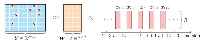
Figure 1: Illustration of TMF on multivariate time series data. For spatiotemporal traffic states data, it can be factorized into spatial factors and temporal factors in which the temporal factor matrix is indeed a multivariate time series. We aim to impose a certain temporal modeling structure on temporal factor matrix.

In time series analysis, one classical approach to achieve stationarity is to perform differencing operators [24]. For example, one can perform first-order differencing and seasonal differencing to transform the original time series data into a stationary copy for model estimation. To characterize the nonstationarity of traffic states data, we propose a parsimonious NoTMF by integrating this differencing operation into the design of temporal loss. For a season-$m$ differencing operation, the transformed temporal loss is given by

$$\frac{1}{2}\sum_{t=d+m+1}^{T}\left\|(\boldsymbol{x}_{t}-\boldsymbol{x}_{t-m})-\sum_{k=1}^{d}\boldsymbol{A}_{k}(\boldsymbol{x}_{t-k}-\boldsymbol{x}_{t-m-k})\right\|_{2}^{2}$$ (3)

$$\equiv \frac{1}{2}\|\boldsymbol{X}\boldsymbol{\Psi}_{0}^{\top}-\boldsymbol{A}(\boldsymbol{I}_{d}\otimes\boldsymbol{X})\boldsymbol{\Psi}^{\top}\|_{F}^{2},$$

where $\boldsymbol{A}=\begin{bmatrix}\boldsymbol{A}_{1}&\cdots&\boldsymbol{A}_{d}\end{bmatrix}\in\mathbb{R}^{R\times(dR)}$ is an augmented matrix. $\boldsymbol{I}_{d}\in\mathbb{R}^{d\times d}$ is an identity matrix, and the symbol $\otimes$ denotes the Kronecker product. We denote by $\boldsymbol{0}_{r\times n}$ an $r\times n$ all-zero matrix, and the temporal operator matrix $\boldsymbol{\Psi}_{k}$ is defined as

$$\boldsymbol{\Psi}_{k}\triangleq \begin{bmatrix}\boldsymbol{0}_{(T-d-m)\times(d-k)}&-\boldsymbol{I}_{T-d-m}&\boldsymbol{0}_{(T-d-m)\times(k+m)}\end{bmatrix}$$ (4)

$$+\begin{bmatrix}\boldsymbol{0}_{(T-d-m)\times(d+m-k)}&\boldsymbol{I}_{T-d-m}&\boldsymbol{0}_{(T-d-m)\times k}\end{bmatrix}$$

$$\in\mathbb{R}^{(T-d-m)\times T},\,\text{ for }k=0,1,\ldots,d,$$

and $\boldsymbol{\Psi}=\begin{bmatrix}\boldsymbol{\Psi}_{1}&\cdots&\boldsymbol{\Psi}_{d}\end{bmatrix}\in\mathbb{R}^{(T-d-m)\times(dT)}$ is an augmented matrix. With this definition, we have a sequence of matrices:

$$\boldsymbol{X}\boldsymbol{\Psi}_{0}^{\top} =\begin{bmatrix}\mid&&\mid\\ \boldsymbol{x}_{d+m+1}-\boldsymbol{x}_{d+1}&\cdots&\boldsymbol{x}_{T}-\boldsymbol{x}_{T-m}\\ \mid&&\mid\\ \end{bmatrix},$$ (5)

$$\boldsymbol{X}\boldsymbol{\Psi}_{1}^{\top} =\begin{bmatrix}\mid&&\mid\\ \boldsymbol{x}_{d+m}-\boldsymbol{x}_{d}&\cdots&\boldsymbol{x}_{T-1}-\boldsymbol{x}_{T-m-1}\\ \mid&&\mid\\ \end{bmatrix},$$

$$~{}~{}\vdots$$

$$\boldsymbol{X}\boldsymbol{\Psi}_{d}^{\top} =\begin{bmatrix}\mid&&\mid\\ \boldsymbol{x}_{m+1}-\boldsymbol{x}_{1}&\cdots&\boldsymbol{x}_{T-d}-\boldsymbol{x}_{T-m-d}\\ \mid&&\mid\\ \end{bmatrix},$$

of size $R\times(T-d-m)$.

The seasonal differencing can help explain seasonality and periodicity underlying the time series data. As a special case, when $m=1$, the temporal modeling operators correspond to first-order differencing. The temporal loss in such case can be written as

$$\frac{1}{2}\sum_{t=d+2}^{T}\left\|(\boldsymbol{x}_{t}-\boldsymbol{x}_{t-1})-\sum_{k=1}^{d}\boldsymbol{A}_{k}(\boldsymbol{x}_{t-k}-\boldsymbol{x}_{t-1-k})\right\|_{2}^{2}.$$ (6)

Thus, the optimization problem of NoTMF takes the form

$$\min_{\boldsymbol{W},\boldsymbol{X},\boldsymbol{A}}{} \frac{1}{2}\|\mathcal{P}_{\Omega}(\boldsymbol{Y}-\boldsymbol{W}^{\top}\boldsymbol{X})\|_{F}^{2}+\frac{\rho}{2}(\|\boldsymbol{W}\|_{F}^{2}+\|\boldsymbol{X}\|_{F}^{2})$$ (7)

$$+\frac{\lambda}{2}\|\boldsymbol{X}\boldsymbol{\Psi}_{0}^{\top}-\boldsymbol{A}(\boldsymbol{I}_{d}\otimes\boldsymbol{X})\boldsymbol{\Psi}^{\top}\|_{F}^{2}.$$

Alternatively, on the top of both seasonal differencing and first-order differencing, the VAR process of NoTMF takes the form:

$$\frac{1}{2}\left\|\boldsymbol{X}\boldsymbol{\Psi}_{0}^{\top}\boldsymbol{\Phi}^{\top}-\sum_{k=1}^{d}\boldsymbol{A}_{k}\boldsymbol{X}\boldsymbol{\Psi}_{k}^{\top}\boldsymbol{\Phi}^{\top}\right\|_{F}^{2},$$ (8)

where $\boldsymbol{\Phi}\triangleq\begin{bmatrix}\boldsymbol{0}_{h\times 1}&\boldsymbol{I}_{h}\end{bmatrix}-\begin{bmatrix}\boldsymbol{I}_{h}&\boldsymbol{0}_{h\times 1}\end{bmatrix}\in\mathbb{R}^{h\times(h+1)},h=T-d-m-1$ refers to the first-order differencing. For complex time series data with both trend and seasonality, achieving stationarity may require more complex operations such as higher-order differencing and differencing with multiple seasonality (e.g., both daily and weekly). VAR process in Eq. (8) can be adapted for certain time series modeling purposes, and the resulting NoTMF is flexible for handling nonstationarity.

We next introduce an alternating minimization framework to solve the optimization problem in NoTMF, in which we denote the objective function of the optimization problem in Eq. (7) by $f$.

3.3 Updating the Spatial Factor Matrix

To learn $\boldsymbol{W}$, we first write down the partial derivative of $f$ with respect to $\boldsymbol{W}$ as follows,

$$\frac{\partial f}{\partial\boldsymbol{W}}=-\boldsymbol{X}\mathcal{P}_{\Omega}^{\top}(\boldsymbol{Y}-\boldsymbol{W}^{\top}\boldsymbol{X})+\rho\boldsymbol{W}.$$ (9)

Let $\frac{\partial f}{\partial\boldsymbol{W}}=\boldsymbol{0}$, then we have

$$\boldsymbol{X}\mathcal{P}_{\Omega}^{\top}(\boldsymbol{W}^{\top}\boldsymbol{X})+\rho\boldsymbol{W}=\boldsymbol{X}\mathcal{P}_{\Omega}^{\top}(\boldsymbol{Y}).$$ (10)

In fact, Eq. (10) represents a system of linear equations, and it is not difficult to obtain the closed-form solution. A natural solution could be pursued through least squares of each column vector of $\boldsymbol{W}$ [20]:

$$\boldsymbol{w}_{i}=\left(\sum_{t:(i,t)\in\Omega}\boldsymbol{x}_{t}\boldsymbol{x}_{t}^{\top}+\rho\boldsymbol{I}_{R}\right)^{-1}\sum_{t:(i,t)\in\Omega}\boldsymbol{x}_{t}y_{it}.$$ (11)

3.4 Updating the Temporal Factor Matrix

As discussed above, we assume a seasonal differencing on the nonstationary temporal factor matrix and claim that such process can promote modeling capability of the matrix factorization framework on time series data. However, the challenge may arise because VAR process on the temporal factor matrix with seasonal differencing complicates the optimization problem. With respect to $\boldsymbol{X}$, the partial derivative is given by

$$\frac{\partial f}{\partial\boldsymbol{X}}= -\boldsymbol{W}\mathcal{P}_{\Omega}(\boldsymbol{Y}-\boldsymbol{W}^{\top}\boldsymbol{X})+\rho\boldsymbol{X}$$ (12)

$$+\lambda\sum_{k=0}^{d}\boldsymbol{A}_{k}^{\top}\left(\sum_{h=0}^{d}\boldsymbol{A}_{h}\boldsymbol{X}\boldsymbol{\Psi}_{h}^{\top}\right)\boldsymbol{\Psi}_{k},$$

where $\boldsymbol{A}_{0}\triangleq-\boldsymbol{I}_{R}$.

Let $\frac{\partial f}{\partial\boldsymbol{X}}=\boldsymbol{0}$, then we have

$$\boldsymbol{W}\mathcal{P}_{\Omega}(\boldsymbol{W}^{\top}\boldsymbol{X})+\rho\boldsymbol{X}$$ (13)

$$+\lambda\sum_{k=0}^{d}\boldsymbol{A}_{k}^{\top}\left(\sum_{h=0}^{d}\boldsymbol{A}_{h}\boldsymbol{X}\boldsymbol{\Psi}_{h}^{\top}\right)\boldsymbol{\Psi}_{k}=\boldsymbol{W}\mathcal{P}_{\Omega}(\boldsymbol{Y}).$$

In fact, Eq. (13) is a generalized Sylvester equation with multiple terms [25]. Since both orthogonal projection and VAR process complicate this matrix equation, if we converts the equation into a standard system of linear equations, then solving the matrix equation would take $\mathcal{O}(R^{3}T^{3})$, as shown in Lemma 1.

Lemma 1.

Given a partially observed data matrix $\boldsymbol{Y}\in\mathbb{R}^{N\times T}$ with the observed index set $\Omega$, the closed-form solution to Eq. (13) in the form of vectorized $\boldsymbol{X}$ is given by

$$\text{vec}(\boldsymbol{X})=\Biggl{(} \boldsymbol{S}+\lambda\sum_{k=0}^{d}\sum_{h=0}^{d}(\boldsymbol{\Psi}_{k}\otimes\boldsymbol{A}_{k})^{\top}(\boldsymbol{\Psi}_{h}\otimes\boldsymbol{A}_{h})$$ (14)

$$+\rho\boldsymbol{I}_{RT}\Biggr{)}^{-1}\text{vec}(\boldsymbol{W}\mathcal{P}_{\Omega}(\boldsymbol{Y})),$$

where $\text{vec}(\cdot)$ denotes the vectorization operator, and $\boldsymbol{S}\triangleq\begin{bmatrix}\boldsymbol{S}_{1}&\boldsymbol{0}&\cdots&\boldsymbol{0}\\ \boldsymbol{0}&\boldsymbol{S}_{2}&\cdots&\boldsymbol{0}\\ \vdots&\vdots&\ddots&\vdots\\ \boldsymbol{0}&\boldsymbol{0}&\cdots&\boldsymbol{S}_{T}\end{bmatrix}\in\mathbb{R}^{(RT)\times(RT)}$ has a sequence of block matrices such that

$$\boldsymbol{S}_{t}\triangleq\sum_{i:(i,t)\in\Omega}\boldsymbol{w}_{i}\boldsymbol{w}_{i}^{\top}\in\mathbb{R}^{R\times R},\,t=1,\ldots,T.$$

However, this vectorized solution is memory-consuming and computationally expensive for large problems. In large applications, as suggested by [23], conjugate gradient method based alternating minimization scheme for matrix factorization provide a solution that is both efficient and scalable. The conjugate gradient method allows one to search for the solution to system of linear equations with a relatively small number of iterations (e.g., 5 or 10). Therefore, to address these problems, we employ an efficient conjugate gradient [25] routine on the temporal factor matrix. We first define an operator as follows,

$$\mathcal{L}_{x}(\boldsymbol{X})\triangleq\text{vec}\Biggl{(} \boldsymbol{W}\mathcal{P}_{\Omega}(\boldsymbol{W}^{\top}\boldsymbol{X})$$ (15)

$$+\lambda\sum_{k=0}^{d}\boldsymbol{A}_{k}^{\top}\Biggl{(}\sum_{h=0}^{d}\boldsymbol{A}_{h}\boldsymbol{X}\boldsymbol{\Psi}_{h}^{\top}\Biggr{)}\boldsymbol{\Psi}_{k}+\rho\boldsymbol{X}\Biggr{)},$$

which is equivalent to

$$\mathcal{L}_{x}(\boldsymbol{X})\equiv\Biggl{(} \boldsymbol{S}+\lambda\sum_{k=0}^{d}\sum_{h=0}^{d}(\boldsymbol{\Psi}_{k}\otimes\boldsymbol{A}_{k})^{\top}(\boldsymbol{\Psi}_{h}\otimes\boldsymbol{A}_{h})$$ (16)

$$+\rho\boldsymbol{I}_{RT}\vphantom{\int_{1}^{2}}\Biggr{)}\text{vec}(\boldsymbol{X}),$$

where $\boldsymbol{S}$ is a sparse matrix as defined in Lemma 1. Since Eq. (16) is in the form of a standard system of linear equations with a symmetric positive-definite matrix, conjugate gradient method is well-suited to such Kronecker structured linear equations. Algorithm 1 summarizes the estimation procedure for approximating the solution to $\boldsymbol{X}$ in Eq. (13). Alternatively, we can also use conjugate gradient to solve Eq. (10) when inferring spatial factor matrix $\boldsymbol{W}$.

Algorithm 1 CGTF$(\boldsymbol{Y},\Omega,\boldsymbol{W},\boldsymbol{X},\{\boldsymbol{\Psi}_{k}\},\boldsymbol{A},d,\lambda,\rho,m,n_{x})$

0:  Data matrix $\boldsymbol{Y}$, $\Omega$ as the observed index set, spatial factor matrix $\boldsymbol{W}$, initialized temporal factor matrix $\boldsymbol{X}$, coefficient matrix $\boldsymbol{A}$, and maximum iteration $n_{x}$ (e.g., $n_{x}=5$).

0:  Estimated temporal factor matrix $\boldsymbol{X}$.

1:  $\boldsymbol{r}_{0}=\text{vec}(\boldsymbol{W}\mathcal{P}_{\Omega}(\boldsymbol{Y}))-\mathcal{L}_{x}(\boldsymbol{X})$, $\boldsymbol{q}_{0}=\boldsymbol{r}_{0}$.

2:  for $\ell=0$ to $n_{x}-1$ do

3:     Convert vector $\boldsymbol{q}_{\ell}$ into matrix $\boldsymbol{Q}_{\ell}$.

4:     Compute $\alpha_{\ell}=\frac{\boldsymbol{r}_{\ell}^{\top}\boldsymbol{r}_{\ell}}{\boldsymbol{q}_{\ell}^{\top}\mathcal{L}_{x}(\boldsymbol{Q}_{\ell})}$.

5:     Update $\boldsymbol{x}_{\ell+1}=\boldsymbol{x}_{\ell}+\alpha_{\ell}\boldsymbol{q}_{\ell}$.

6:     Update $\boldsymbol{r}_{\ell+1}=\boldsymbol{r}_{\ell}-\alpha_{\ell}\mathcal{L}_{x}(\boldsymbol{Q}_{\ell})$.

7:     Compute $\beta_{\ell}=\frac{\boldsymbol{r}_{\ell+1}^{\top}\boldsymbol{r}_{\ell+1}}{\boldsymbol{r}_{\ell}^{\top}\boldsymbol{r}_{\ell}}$.

8:     Update $\boldsymbol{q}_{\ell+1}=\boldsymbol{r}_{\ell+1}+\beta_{\ell}\boldsymbol{q}_{\ell}$.

9:  end for

10:  Convert vector $\boldsymbol{x}_{n_{x}}$ into matrix $\boldsymbol{X}$.

11:  return  Temporal factor matrix $\boldsymbol{X}$.

3.5 Updating the Coefficient Matrix

Regarding the coefficient matrix $\boldsymbol{A}$, the partial derivative can be written as

$$\frac{\partial f}{\partial\boldsymbol{A}}=-\lambda(\boldsymbol{X}\boldsymbol{\Psi}_{0}^{\top}-\boldsymbol{A}(\boldsymbol{I}_{d}\otimes\boldsymbol{X})\boldsymbol{\Psi}^{\top})\boldsymbol{\Psi}(\boldsymbol{I}_{d}\otimes\boldsymbol{X})^{\top}.$$ (17)

Let $\frac{\partial f}{\partial\boldsymbol{A}}=\boldsymbol{0}$, then we have a least squares solution to the coefficient matrix:

$$\boldsymbol{A}= \lambda\boldsymbol{X}\boldsymbol{\Psi}_{0}^{\top}\boldsymbol{\Psi}(\boldsymbol{I}_{d}\otimes\boldsymbol{X})^{\top}\left(\lambda(\boldsymbol{I}_{d}\otimes\boldsymbol{X})\boldsymbol{\Psi}^{\top}\boldsymbol{\Psi}(\boldsymbol{I}_{d}\otimes\boldsymbol{X})^{\top}\right)^{-1}$$ (18)

$$\equiv \boldsymbol{X}\boldsymbol{\Psi}_{0}^{\top}[(\boldsymbol{I}_{d}\otimes\boldsymbol{X})\boldsymbol{\Psi}^{\top}]^{\dagger},$$

where $\cdot^{\dagger}$ denotes the Moore-Penrose pseudo-inverse.

3.6 Solution Algorithm

Algorithm 2 NoTMF$(\boldsymbol{Y},\Omega,d,R,\lambda,\rho,m,n,n_{x})$

0:  Data matrix $\boldsymbol{Y}$, $\Omega$ as the observed index set, $d$ as the order of VAR, $R$ as the low rank, and maximum iteration $n$.

0:  Spatial factor matrix $\boldsymbol{W}$, temporal factor matrix $\boldsymbol{X}$, and coefficient matrix $\boldsymbol{A}$.

1:  Initialize $\boldsymbol{W}_{0},\boldsymbol{X}_{0},\boldsymbol{A}_{0}$.

2:  Generate temporal modeling operators $\{\boldsymbol{\Psi}_{k}\}$.

3:  for $\ell=0$ to $n-1$ do

4:     Compute $\boldsymbol{W}_{\ell+1}$ by the least squares solution (or conjugate gradient).

5:     Compute $\boldsymbol{X}_{\ell+1}=\text{CGTF}(\boldsymbol{Y},\Omega,\boldsymbol{W}_{\ell+1},\boldsymbol{X}_{\ell},\{\boldsymbol{\Psi}_{k}\},$ $\boldsymbol{A}_{\ell},d,\lambda,\rho,m,n_{x})$.

6:     Compute $\boldsymbol{A}_{\ell+1}$ by the least squares solution.

7:  end for

8:  return  $\boldsymbol{W}_{n},\boldsymbol{X}_{n},\boldsymbol{A}_{n}$.

We summarize the implementation of NoTMF in Algorithm 2. We next introduce a forecasting scheme for NoTMF. As $\boldsymbol{W},\boldsymbol{X},\boldsymbol{A}$ are estimated through training Algorithm 2, one can first perform seasonal differencing on $\boldsymbol{x}_{1},\ldots,\boldsymbol{x}_{T}$ (i.e., columns of temporal facror matrix) as $\boldsymbol{v}_{1}=\boldsymbol{x}_{m+1}-\boldsymbol{x}_{1},\ldots,\boldsymbol{v}_{T-m}=\boldsymbol{x}_{T}-\boldsymbol{x}_{T-m}$, then estimate the forecasts $\hat{\boldsymbol{v}}_{T-m+1},\ldots,\hat{\boldsymbol{v}}_{T-m+\delta}$ with the coefficient matrix $\boldsymbol{A}$ at the time horizon $\delta\in\mathbb{N}^{+}$. Finally, we can generate the forecasts $\hat{\boldsymbol{y}}_{T+1},\ldots,\hat{\boldsymbol{y}}_{T+\delta}$ sequentially by

$$\hat{\boldsymbol{y}}_{T+1} =\boldsymbol{W}^{\top}(\boldsymbol{x}_{T-m}+\hat{\boldsymbol{v}}_{T-m}),$$ (19)

$$\,\,\,\vdots$$

$$\hat{\boldsymbol{y}}_{T+\delta} =\boldsymbol{W}^{\top}(\hat{\boldsymbol{x}}_{T-m-1+\delta}+\hat{\boldsymbol{v}}_{T-m-1+\delta}).$$

3.7 Rolling Forecasting Mechanism

In our implementation, we consider a rolling forecasting scheme for spatiotemporal traffic states data. We denote the incremental data at the $s$th rolling forecasting with the time horizon $\delta$ by $\boldsymbol{Y}_{s}\in\mathbb{R}^{N\times(T+(s-1)\cdot\delta)}$. NoTMF can process the entire data at once but it is impractical to accommodate data arriving sequentially. Therefore, we take into account the dictionary learning with fixed spatial factor matrix (also examined in [17]). Such a collection of spatial factors enables the system to reformat the incremental sparse data to lower-dimensional temporal factors. In each rolling scheme, we first learn temporal factor matrix through conjugate gradient method, which is computationally efficient. Then we update the coefficient matrix accordingly for capturing time-evolving patterns. Algorithm 3 shows the whole scheme of rolling forecasting on the multivariate traffic states data.

Algorithm 3 NoTMF Forecasting with Missing Values

0:  Data matrix $\boldsymbol{Y}\in\mathbb{R}^{N\times T}$, $\Omega$ as the observed index set, $d$ as the order of VAR, $R$ as the low rank, $S$ as the number of rolling times, and $\delta$ as the forecasting time horizon.

0:  Forecasts $\hat{\boldsymbol{Y}}\in\mathbb{R}^{N\times\delta\cdot S}$.

1:  Train NoTMF on data matrix $\boldsymbol{Y}$ and return the result:$\boldsymbol{W},\boldsymbol{X},\boldsymbol{A}=\text{NoTMF}(\boldsymbol{Y},\Omega,d,R,\lambda,\rho,m,n,n_{x})$.

2:  Generate the forecasts $\hat{\boldsymbol{y}}_{T+1},\ldots,\hat{\boldsymbol{y}}_{T+\delta}$ by Eq. (19) and stack them as the first $\delta$ columns of $\hat{\boldsymbol{Y}}$.

3:  for $s=2$ to $S$ do

4:     Input the incremental data $\boldsymbol{Y}_{s}\in\mathbb{R}^{N\times(T+(s-1)\cdot\delta)}$ in which the last $\delta$ columns are the newly arriving data.

5:     Generate temporal modeling operators $\{\boldsymbol{\Psi}_{k}\}$.

6:     Compute $\boldsymbol{X}_{s}=\text{CGTF}(\boldsymbol{Y}_{s},\Omega_{s},\boldsymbol{W},\boldsymbol{X},\{\boldsymbol{\Psi}_{k}\},\boldsymbol{A},d,$ $\lambda,\rho,m,n_{x})$.

7:     Update the coefficient matrix $\boldsymbol{A}$.

8:     Generate the forecasts: $\hat{\boldsymbol{y}}_{T+(s-1)\cdot\delta+1},\ldots,\hat{\boldsymbol{y}}_{T+(s-1)\cdot\delta+\delta}$ and stack them to $\hat{\boldsymbol{Y}}$.

9:  end for

10:  return  $\hat{\boldsymbol{Y}}$.

4 Experiments

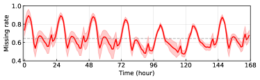
(a) NYC Uber hourly movement speed data.

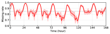
(b) Seattle Uber hourly movement speed data.

Figure 2: The missing rates of Uber movement speed data aggregated per week over the whole year of 2019. The red curve shows the average missing rates over all 52 weeks. The red area shows the standard deviation of missing rates in each hour over 52 weeks. The 168 time steps refer to 168 hours of Tuesday, Wednesday, Thursday, Friday, Saturday, Sunday, and Monday. (a) The dataset has 98,210 road segments, and the overall hourly missing rate is 64.43%. (b) The dataset has 63,490 road segments, and the whole missing rate is 84.95%.

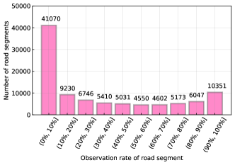
Figure 3: Histogram of observation rate of road segment in the NYC Uber movement speed dataset. Only a small fraction of road segments has observation rate greater than 50%, i.e., $30723/98210\approx 31\%$. For the observation rates greater than 20% and 80%, there are about 49% and 17% of road segments, respectively.

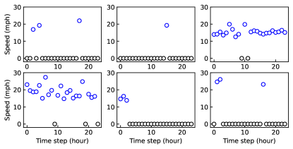
Figure 4: Movement speed of 6 road segments of January 1st, 2019 (24 hours) in NYC. Blue scatters indicate the movement speed data points, and data points with value 0 (i.e., black scatters) indicate the missing values.

In this section, we evaluate the performance of NoTMF on a large traffic speed dataset collected from urban road networks—the New York City (NYC) Uber movement speed dataset. To verify the effectiveness of NoTMF, we also conduct complementary experiments on other datasets (see Appendix A for details). We use the mean absolute percentage error (MAPE) and root mean square error (RMSE) as performance metrics:

MAPE $$=\frac{1}{n}\sum_{i=1}^{n}\frac{|y_{i}-\hat{y}_{i}|}{y_{i}}\times 100,$$ (20)

RMSE $$=\sqrt{\frac{1}{n}\sum_{i=1}^{n}(y_{i}-\hat{y}_{i})^{2}},$$

where $n$ is the total number of estimated values, and $y_{i}$ and $\hat{y}_{i}$ are the actual value and its estimate, respectively.

4.1 Data and Experiment Setup

The data is taken from Uber movement project. The project provides the average speed on a given road segment in urban areas for each hour of each day over the study period. Uber movement speed data is a representative example for illustrating both high-dimensionality and sparsity issues in real-world time series data. Fig. 2 shows two cases of Uber movement speed data in NYC and Seattle, USA, respectively. The high-dimensional and sparse data inevitably result in difficulties of analyzing traffic states or supporting decision-making.

We use the NYC Uber movement speed data collected from 98,210 road segments during the first ten weeks of 2019 for the following experiments, and this dataset is of size $98210\times 1680$. Due to the mechanism of insufficient sampling of ridesharing vehicles on urban road networks, the dataset contains 66.56% missing values. It can be seen that the time-evolving missing rates have periodicity patterns. In the middle of the night, the missing rate can even reach $\sim$90%. This is due to limited ridesharing vehicles on the road network during the midnight. At any specific hour, only a small fraction of road segments have speed observations.

Fig. 3 shows the complementary histogram of the percentage of observed value in the data set. As can be seen, a large fraction of road segments only have limited observations. This is especially interesting, as it shows that half the road segments have less than 20% movement speed observations. Only 17% road segments have more than 80% movement speed observations. We can also see the incomplete movement speed observations from Fig. 4.

In our experiment, we evaluate the model with 8-week data (from January $1$st to February $25$th) as training set, one-week data (February $26$th to March $4$th) for validation, and one-week data (March $5$th to March $11$th) for test. We use the rolling forecasting with time horizons $\delta=1,2,3,6$, corresponding to $\delta$-hour-ahead forecasting. We evaluate NoTMF against the following baseline models:

• TMF: This is the foundation of our NoTMF model, and it applies VAR to the temporal factor matrix without seasonal differencing following Eq. (2).

• TRMF [5]: TRMF achieves temporal modeling on latent temporal factors by applying univariate autoregressive process, and it is a special case of the general TMF as discussed in Eq. (7).

• BTMF [7]: Bayesian Temporal Matrix Factorization (BTMF) is a fully Bayesian TMF model with Gaussian assumption, which is solved by using Markov chain Monte Carlo algorithm.

• BTRMF: Bayesian TRMF is a fully Bayesian treatment for TRMF model with Gaussian assumption.

TMF is the most important baseline, since the comparison between TMF and NoTMF will reveal the importance of explicitly modeling seasonality through differencing. We implement these models using the NumPy library in Python and all experiments were conducted on a desktop with $8$ cores i7-9700 CPU and $16$GB RAM. The adapted dataset and Python implementation (both CPU and GPU) are available at https://github.com/xinychen/tracebase.

4.2 Forecasting Performance

We evaluate the task of multivariate time series forecasting in the presence of missing data on the NYC Uber movement speed dataset. The preliminary experiment evaluates the NoTMF model with different ranks $R=5,10,15,20,25,30$. As shown in Fig. 5, a larger rank essentially provides higher accuracy but the increase becomes marginal when $R>15$. In the following experiments, we choose $R=10$ for a good balance between performance and computational cost.

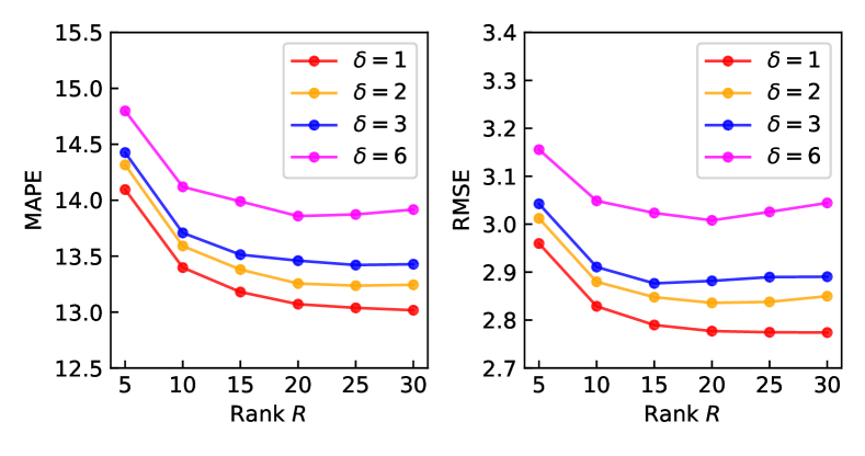
Figure 5: Performance of NoTMF with season-168 differencing (i.e., $m=168$) and order $d=6$. The validated parameters are $\lambda=1$ and $\rho=5$.

TABLE I: Forecasting performance (MAPE/RMSE) on the NYC movement speed dataset. The rolling forecasting tasks include different time horizons, i.e., $\delta=1,2,3,6$. We consider the rank as $R=10$. After the cross validation for finding best $(\lambda,\rho)$, we set $(\lambda,\rho)$ as $(1,5)$ for NoTMF, TMF, and TRMF. Note that best results are highlighted in bold fonts.

$\delta$	$d$	NoTMF ($m=24$)	NoTMF  ($m=168$)	NoTMF-1st  ($m=168$)	TMF	TRMF	BTMF	BTRMF
1	1	13.63/2.88	13.53/2.86	13.45/2.85	13.74/2.90	14.50/3.12	14.94/3.13	15.93/3.33
	2	13.47/2.84	13.41/2.84	13.42/2.84	13.53/2.85	14.14/3.05	15.70/3.41	15.90/3.35
	3	13.46/2.84	13.39/2.83	13.43/2.84	13.47/2.83	13.87/2.96	15.80/3.34	16.08/3.43
	6	13.41/2.83	13.39/2.83	13.41/2.83	13.40/2.83	14.00/2.98	15.45/3.27	16.26/3.48
2	1	13.91/2.96	13.76/2.94	13.70/2.92	14.24/3.00	15.85/3.43	15.33/3.21	16.85/3.56
	2	13.77/2.92	13.63/2.89	13.72/2.92	13.87/2.91	15.04/3.31	15.87/3.32	17.27/3.71
	3	13.72/2.91	13.61/2.89	13.73/2.92	13.81/2.89	15.25/3.36	15.69/3.33	17.24/3.74
	6	13.59/2.87	13.57/2.88	13.68/2.91	13.63/2.86	14.92/3.24	15.91/3.39	18.18/3.97
3	1	14.30/3.05	14.06/3.02	14.02/3.00	14.81/3.12	17.52/3.83	15.86/3.32	18.61/3.91
	2	14.01/2.98	13.84/2.94	13.96/2.98	14.26/2.98	17.32/4.00	16.30/3.40	18.90/4.10
	3	13.95/2.97	13.79/2.93	13.98/2.98	14.04/2.94	16.91/3.71	16.56/3.49	18.68/4.05
	6	13.78/2.92	13.73/2.92	13.91/2.96	13.94/2.92	16.72/3.65	15.49/3.27	20.45/4.66
6	1	14.61/3.11	14.67/3.20	14.98/3.32	15.41/3.21	21.20/4.70	15.99/3.32	22.40/4.69
	2	14.30/3.03	14.33/3.09	14.90/3.28	14.85/3.07	20.87/5.01	16.04/3.33	23.56/5.63
	3	14.26/3.03	14.28/3.09	14.86/3.26	14.57/3.01	20.08/4.65	15.67/3.28	24.27/5.72
	6	14.06/2.97	14.16/3.06	14.80/3.23	14.47/3.00	20.40/4.35	16.38/3.50	26.34/6.60

Table I shows the forecasting performance of NoTMF and baseline models. We summarize the following findings from the results:

• With the increase of forecasting time horizons, the forecasting errors of all models increase. For each time horizon, as the order becomes greater, the forecasting performance of NoTMF, TMF, and TRMF is improved.

• Both NoTMF and TMF models demonstrate a significant improvement over TRMF with respect to the forecasting accuracy. In contrast to the univariate autoregressive process, there is a clear benefit from temporal modeling with multivariate VAR process.

• Putting the results of NoTMF and TMF together for comparison, it shows that NoTMF outperforms TMF in most cases. If $d$ is a relatively small value (e.g., $d=1,2,3$), then the forecasting results of NoTMF are significantly better than those of TMF. The result further confirms the importance of seasonal differencing in NoTMF.

• On this dataset, we have two choices for setting the season, one is $m=24$, corresponding to the daily differencing; another is $m=168$, corresponding to the weekly differencing. For both two settings, NoTMF can achieve competitively accurate forecasts.

• NoTMF-1st represents the NoTMF model with both seasonal differencing and first-order differencing (see the VAR process in Eq. (8)), and it performs better than NoTMF ($m=168$) when the order $d$ is relatively small.

Fig. 6 shows the predicted and actual values of some road segments. It demonstrates that the forecasting from NoTMF is consistent with the temporal patterns underlying partially observed time series. Thus, the NoTMF model can extract out implicit temporal patterns (see Fig. 7 for instance) from partially observed data and perform forecasting.

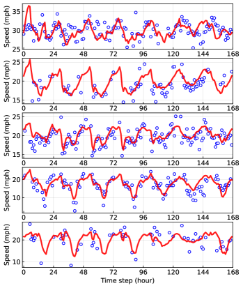
Figure 6: Five examples (corresponding to five road segments) for showing the forecasting results of NoTMF model with time horizon $\delta=6$. The red curves indicate the forecasts in the testing week, while the blue scatters indicate the ground truth speed data.

4.3 Analysis on Conjugate Gradient Method

TABLE II: Forecasting performance (MAPE/RMSE) of NoTMF with different conjugate gradient iterations on the NYC movement speed dataset. The rank and season of NoTMF are set as $R=10$ and $m=168$, respectively.

$\delta$	$d$	3 iters.	5 iters.	10 iters.	15 iters.
1	1	13.57/2.88	13.53/2.86	13.55/2.87	13.69/2.94
	2	13.45/2.85	13.41/2.84	13.42/2.84	13.41/2.83
	3	13.45/2.85	13.39/2.83	13.39/2.83	13.41/2.83
	6	13.44/2.84	13.39/2.83	13.38/2.83	13.38/2.83
2	1	13.82/2.96	13.76/2.94	13.79/2.94	13.80/2.94
	2	13.64/2.90	13.63/2.89	13.62/2.89	13.62/2.89
	3	13.62/2.90	13.61/2.89	13.59/2.89	13.60/2.89
	6	13.57/2.89	13.57/2.88	13.56/2.88	13.56/2.88
3	1	14.16/3.05	14.06/3.02	14.06/3.01	14.06/3.01
	2	13.91/2.97	13.84/2.94	13.81/2.94	13.81/2.93
	3	13.84/2.95	13.79/2.93	13.75/2.92	13.75/2.92
	6	13.76/2.93	13.73/2.92	13.68/2.91	13.69/2.91
6	1	14.68/3.20	14.67/3.20	14.75/3.21	14.77/3.22
	2	14.46/3.12	14.33/3.09	14.31/3.08	14.32/3.09
	3	14.44/3.12	14.28/3.09	14.23/3.07	14.24/3.07
	6	14.34/3.10	14.16/3.06	14.11/3.04	14.11/3.05

In this work, conjugate gradient method is used as an efficient procedure to approximate the solution to the factor matrix from generalized Sylvester equation. One advantage is that the iterative process of conjugate gradient method does not require too many iterations to reach convergence. Previous studies also evaluated conjugate gradient method by comparing to gradient descent method and demonstrated the efficiency and effectiveness of conjugate gradient method [23]. Table II shows the forecasting performance of NoTMF with different conjugate gradient iterations. It demonstrates that NoTMF with $5$ conjugate gradient iterations can already achieve good accuracy, and the improvement with more iterations becomes marginal. In addition, conjugate gradient method brings benefits to NoTMF in terms of both efficiency and scalability. In our experiment, the training process of NoTMF ($m=168$) on the first $9$-week data of NYC movement speed dataset with different orders (i.e., $d=1,2,3,6$) and rank $R=10$ only takes a few seconds, which seems to be efficient for our large-scale problems.

4.4 Nonstationarity Analysis

Nonstationarity is an important characteristic in most real-world time series data. Fig. 7 illustrates some temporal factors of NoTMF with the following setting: $d=1$, $R=10$, and $m=24$. As can be seen, temporal factors #3, #5, #6, #7, #8, and #9 show clear seasonality and periodicity. The long-term season is associated with week, i.e., $7\times 24=168$ time steps (hours), while the short-term season is associated with day, i.e., $24$ time steps (hours). For other temporal factors, they also show clear trends with weak seasonality and periodicity. Therefore, making use of seasonal differencing in nonstationary traffic states data can benefit the forecasting performance (as noted in Table I). Our results further demonstrate the effectiveness of seasonal differencing operations in characterizing temporal process in $\boldsymbol{X}$.

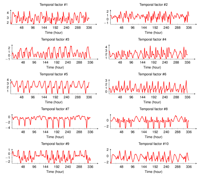
Figure 7: Temporal factors of NoTMF model ($R=10$) on NYC movement speed data. The order and season of NoTMF are set as $d=1$ and $m=24$, respectively. The subfigures only show the temporal factors in the first two weeks.

5 Conclusion and Future Work

In this paper, we propose NoTMF for forecasting on high-dimensional, sparse, and nonstationary time series data. NoTMF is an extension of TMF by integrating differencing operations on the latent temporal factors. We develop a consistent approach to model the temporal loss using matrix operations, and this allows to solve the complex optimization problem through conjugate gradient method. The conjugate gradient method is an efficient and scalable routine for inferring factor matrix from generalized Sylvester equation. Therefore, the algorithms developed in this work can support efficient time series modeling/forecasting on high-dimensional and large-scale time series data. The extensive numerical experiments on Uber movement speed dataset confirm the superior performance of NoTMF over baseline models, and the comparison with TMF shows the advantage of addressing the nonstationary issue before modeling time series with clear seasonality and trend.

Appendix A Additional Experiments

TABLE III: Forecasting performance (MAPE/RMSE) on both Seattle movement speed dataset. The rolling forecasting tasks include different time horizons, i.e., $\delta=1,2,3,6$. We consider the rank as $R=10$. After the cross validation for finding best $(\lambda,\rho)$, we set $(\lambda,\rho)$ as $(1,5)$ for NoTMF, TMF, and TRMF. Note that best results are highlighted in bold fonts.

$\delta$	$d$	NoTMF ($m=24$)	NoTMF  ($m=168$)	NoTMF-1st  ($m=168$)	TMF	TRMF	BTMF	BTRMF
1	1	10.45/3.32	10.26/3.22	10.26/3.21	10.70/3.37	11.58/3.79	12.23/3.89	12.52/4.01
	2	10.53/3.34	10.29/3.23	10.23/3.21	10.47/3.28	10.92/3.51	12.95/4.18	13.16/4.31
	3	10.42/3.30	10.30/3.22	10.25/3.21	10.40/3.27	10.86/3.47	12.96/4.22	13.89/4.64
	6	10.50/3.32	10.21/3.21	10.27/3.22	10.32/3.24	10.99/3.51	12.91/4.18	13.90/4.67
2	1	10.90/3.55	10.32/3.25	10.25/3.23	11.11/3.52	12.07/4.02	12.74/4.06	13.31/4.32
	2	10.90/3.52	10.31/3.24	10.25/3.23	10.99/3.48	12.59/4.24	13.68/4.45	13.44/4.43
	3	10.81/3.49	10.31/3.24	10.27/3.23	10.75/3.40	12.01/3.96	13.55/4.46	13.66/4.56
	6	10.57/3.38	10.25/3.23	10.27/3.23	10.69/3.38	12.18/3.98	13.56/4.42	14.67/4.92
3	1	11.27/3.71	10.41/3.29	10.41/3.29	11.80/3.77	13.47/4.62	13.16/4.15	14.01/4.52
	2	11.26/3.71	10.30/3.27	10.34/3.27	11.93/3.83	14.48/5.19	13.63/4.37	14.39/4.76
	3	11.11/3.62	10.35/3.28	10.38/3.28	11.62/3.70	14.04/4.83	13.76/4.42	14.67/4.84
	6	10.96/3.55	10.30/3.26	10.30/3.26	11.07/3.52	13.32/4.51	13.28/4.29	15.64/5.31
6	1	11.88/3.97	10.63/3.43	10.60/3.42	13.17/4.18	15.59/5.32	13.63/4.30	16.39/5.28
	2	11.58/3.83	10.55/3.40	10.56/3.40	12.61/3.99	18.66/7.20	13.27/4.19	16.77/5.58
	3	11.54/3.81	10.57/3.39	10.53/3.38	12.22/3.85	17.94/6.32	13.88/4.36	17.35/5.70
	6	11.27/3.70	10.53/3.35	10.50/3.35	11.37/3.59	15.12/5.24	13.30/4.24	16.63/5.62

TABLE IV: Forecasting performance (MAPE/RMSE) of NoTMF and TMF models on both the JERICHO-E-usage dataset and the Google Flu Trends dataset. Note that the RMSE values for JERICHO-E-usage dataset are with an increase of $5$ orders of magnitude, i.e., $\times 10^{5}$. For JERICHO-E-usage dataset, the rank of NoTMF is set as $10$, the validated parameters are $\lambda=10$ and $\rho=0.5$. For Google Flu Trends dataset, the rank of NoTMF is set as $10$, the validated parameters are $\lambda=5$ and $\rho=0.5$.

$\delta$	$d$	JERICHO-E-usage dataset				Google Flu Trends dataset
		NoTMF  ($m=24$)	NoTMF  ($m=168$)	TMF  (baseline)	TRMF  (baseline)	NoTMF  ($m=1$)	NoTMF  ($m=52$)	TMF  (baseline)	TRMF  (baseline)
2	1	54.46/1.63	41.33/1.12	69.80/1.69	67.30/1.81	21.66/1071	23.41/1183	22.21/1111	21.78/1227
	2	52.27/1.62	42.74/1.10	62.72/1.57	62.04/1.89	22.06/1070	23.17/1130	22.47/1066	21.25/1034
	3	65.50/1.63	50.62/1.09	61.69/1.52	60.62/1.93	22.81/1105	24.13/1102	22.49/1034	20.58/1085
	6	55.78/1.52	52.74/1.09	71.10/1.40	49.30/1.84	-/-	-/-	-/-	-/-
3	1	47.57/1.74	38.88/1.22	120.16/1.94	78.96/2.25	24.22/1468	25.19/1219	24.26/1322	23.10/1384
	2	56.08/1.71	40.70/1.16	99.82/1.82	120.31/2.15	25.19/1488	25.67/1332	25.35/1342	32.30/1527
	3	63.91/1.71	44.74/1.13	102.55/1.73	73.23/2.10	25.77/1478	25.42/1250	24.55/1341	28.42/1455
	6	84.55/1.58	41.98/1.13	98.05/1.49	103.50/2.16	-/-	-/-	-/-	-/-
4	1	42.25/1.83	39.50/1.28	147.75/1.94	117.01/2.32	25.42/1313	26.14/1215	25.18/1266	27.74/1698
	2	46.17/1.81	41.19/1.24	104.24/1.84	68.28/2.39	26.71/1335	25.97/1212	26.80/1212	38.82/1867
	3	68.04/1.79	47.32/1.22	114.74/1.76	129.46/2.30	27.45/1348	26.92/1257	25.60/1221	30.79/1631
	6	78.64/1.68	42.87/1.21	92.84/1.57	103.71/2.23	-/-	-/-	-/-	-/-

To verify the effectiveness of NoTMF, we also evaluate the forecasting approaches on the following three datasets:

• Seattle movement speed dataset. This dataset is also taken from Uber movement project (as mentioned in Fig. 2), which covers the hourly movement speed data from 63,490 road segments during the first ten weeks of 2019. The data matrix is of size $63490\times 1680$ and contains 87.35% missing values.

• JERICHO-E-usage dataset. This is an energy consumption time series dataset provided in [26]. This dataset covers the hourly energy consumption of $38$ regions in Germany with different energy categories (e.g., residential, industrial, commerce, and mobility sectors) in the whole year of 2019. All $1178$ energy consumption time series are of length $8760$ (i.e., $24\times 365$). We use the subset in the first ten weeks for experiments, which is of size $1178\times 1680$.

• Google Flu Trends dataset. This is a time series dataset which consists of weekly estimates (i.e., weekly time resolution) of influenza activity based on volume of certain search queries from 2003 to 2015 (see Fig. 8) [27]. This dataset covers 97 US cities, and the time series is of size $97\times 620$. There are about 3.18% missing values in the time series data.

On Seattle movement speed dataset, we conduct rolling time series forecasting and compare the proposed NoTMF with some baseline models as shown in Table III. Of these results, NoTMF consistently outperforms other models. We set NoTMF with both daily differencing (i.e., $m=24$) and weekly differencing (i.e., $m=168$), and it shows that the weekly differencing is superior to the daily differencing. Therefore, a suitable seasonal differencing in NoTMF is important for improving the forecasting performance.

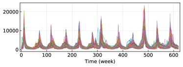
Figure 8: Total 97 time series curves of Google Flu Trends dataset.

On JERICHO-E-usage dataset, we separate $8$-week data as the training sets, one-week data for validation, and the remaining one-week data for test. In particular, we randomly remove $50\%$ observations as the missing portion to evaluate the time series forecasting with missing values. On Google Flu Trends dataset, we separate $412$-week data for training, $52$-week data for validation, and the remaining $156$-week data for test.

Table IV shows the forecasting performance achieved by NoTMF, TMF, and TRMF models on both two datasets. As can be seen, NoTMF outperforms TMF significantly. For JERICHO-E-usage dataset, the superior performance of NoTMF with season-168 differencing (i.e., weekly differencing) over NoTMF with season-24 differencing (i.e., daily differencing) demonstrates that an appropriate seasonal differencing is vital for the success of NoTMF. Fig. 9 shows the aggregated energy consumption of forecasting results of NoTMF. For Google Flu Trends dataset, the performance with season-1 differencing (i.e., first-order differencing) and season-52 differencing outperforms both TMF and TRMF in most cases, demonstrating the effectiveness of nonstationarity modeling through seasonal differencing in NoTMF.

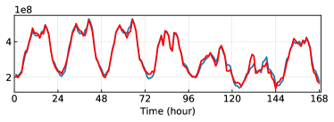
Figure 9: The aggregated energy consumption of forecasting results of NoTMF model with time horizon $\delta=4$. The red curve indicates the sum of forecasts in the testing week, while the blue curve indicates the aggregated energy of ground truth data.

Xinyu Chen received the B.S. degree in Traffic Engineering from Guangzhou University, Guangzhou, China, in 2016, and M.S. degree in Transportation Information Engineering & Control from Sun Yat-Sen University, Guangzhou, China, in 2019. He is currently a Ph.D. student with the Civil, Geological and Mining Engineering Department, Polytechnique Montreal, Montreal, QC, Canada. His current research centers on machine learning, spatiotemporal data modeling, and intelligent transportation systems.

Chengyuan Zhang is a Ph.D. student with the Department of Civil Engineering, McGill University, Montreal, QC, Canada. He received his B.S. degree in Automotive Engineering from Chongqing University, Chongqing, China, in 2019. His research interests include machine learning, macro/micro driving behavior modeling and prediction, multi-agent interaction, and intelligent vehicles.

Xi-Le Zhao received the M.S. and Ph.D. degrees from the University of Electronic Science and Technology of China (UESTC), Chengdu, China, in 2009 and 2012, respectively. He is currently a Professor with the School of Mathematical Sciences, UESTC. His research interests mainly focus on model-driven and data-driven methods for image processing problems. His homepage is https://zhaoxile.github.io.

Nicolas Saunier received an engineering degree and a Doctorate (Ph.D.) in computer science from Telecom ParisTech, Paris, France, respectively in 2001 and 2005. He is currently a Full Professor with the Civil, Geological and Mining Engineering Department at Polytechnique Montreal, Montreal, QC, Canada. His research interests include intelligent transportation, road safety, and data science for transportation.

Lijun Sun received the B.S. degree in Civil Engineering from Tsinghua University, Beijing, China, in 2011, and Ph.D. degree in Civil Engineering (Transportation) from National University of Singapore in 2015. He is currently an Assistant Professor with the Department of Civil Engineering at McGill University, Montreal, QC, Canada. His research centers on intelligent transportation systems, machine learning, spatiotemporal modeling, travel behavior, and agent-based simulation. He is a member of the IEEE.

References

- [1] H. Lütkepohl, Introduction to multiple time series analysis. Springer Science & Business Media, 2013.
- [2] M. Verleysen and D. François, “The curse of dimensionality in data mining and time series prediction,” in International work-conference on artificial neural networks. Springer, 2005, pp. 758–770.
- [3] S. Basu, X. Li, and G. Michailidis, “Low rank and structured modeling of high-dimensional vector autoregressions,” IEEE Transactions on Signal Processing, vol. 67, no. 5, pp. 1207–1222, 2019.
- [4] D. Wang, Y. Zheng, H. Lian, and G. Li, “High-dimensional vector autoregressive time series modeling via tensor decomposition,” Journal of the American Statistical Association, pp. 1–19, 2021.
- [5] H.-F. Yu, N. Rao, and I. S. Dhillon, “Temporal regularized matrix factorization for high-dimensional time series prediction,” Advances in neural information processing systems, vol. 29, pp. 847–855, 2016.
- [6] L. Xiong, X. Chen, T.-K. Huang, J. Schneider, and J. G. Carbonell, “Temporal collaborative filtering with bayesian probabilistic tensor factorization,” in Proceedings of the 2010 SIAM international conference on data mining. SIAM, 2010, pp. 211–222.
- [7] X. Chen and L. Sun, “Bayesian temporal factorization for multidimensional time series prediction,” IEEE Transactions on Pattern Analysis and Machine Intelligence, 2021.
- [8] J. H. Stock and M. W. Watson, “Dynamic factor models, factor-augmented vector autoregressions, and structural vector autoregressions in macroeconomics,” in Handbook of macroeconomics. Elsevier, 2016, vol. 2, pp. 415–525.
- [9] R. P. Velu, G. C. Reinsel, and D. W. Wichern, “Reduced rank models for multiple time series,” Biometrika, vol. 73, no. 1, pp. 105–118, 1986.
- [10] R. Velu and G. C. Reinsel, Multivariate reduced-rank regression: theory and applications. Springer Science & Business Media, 1998, vol. 136.
- [11] S. Basu and G. Michailidis, “Regularized estimation in sparse high-dimensional time series models,” The Annals of Statistics, vol. 43, no. 4, pp. 1535–1567, 2015.
- [12] A. Carriero, G. Kapetanios, and M. Marcellino, “Structural analysis with multivariate autoregressive index models,” Journal of Econometrics, vol. 192, no. 2, pp. 332–348, 2016.
- [13] G. Koop, D. Korobilis, and D. Pettenuzzo, “Bayesian compressed vector autoregressions,” Journal of Econometrics, vol. 210, no. 1, pp. 135–154, 2019.
- [14] F. Han, H. Lu, and H. Liu, “A direct estimation of high dimensional stationary vector autoregressions,” Journal of Machine Learning Research, 2015.
- [15] Z. Che, S. Purushotham, K. Cho, D. Sontag, and Y. Liu, “Recurrent neural networks for multivariate time series with missing values,” Scientific reports, vol. 8, no. 1, pp. 1–12, 2018.
- [16] K. Takeuchi, H. Kashima, and N. Ueda, “Autoregressive tensor factorization for spatio-temporal predictions,” in 2017 IEEE International Conference on Data Mining (ICDM). IEEE, 2017, pp. 1105–1110.
- [17] S. Gultekin and J. Paisley, “Online forecasting matrix factorization,” IEEE Transactions on Signal Processing, vol. 67, no. 5, pp. 1223–1236, 2018.
- [18] D. M. Dunlavy, T. G. Kolda, and E. Acar, “Temporal link prediction using matrix and tensor factorizations,” ACM Transactions on Knowledge Discovery from Data (TKDD), vol. 5, no. 2, pp. 1–27, 2011.
- [19] K. Kawabata, S. Bhatia, R. Liu, M. Wadhwa, and B. Hooi, “Ssmf: Shifting seasonal matrix factorization,” Advances in Neural Information Processing Systems, vol. 34, 2021.
- [20] Y. Koren, R. Bell, and C. Volinsky, “Matrix factorization techniques for recommender systems,” Computer, vol. 42, no. 8, pp. 30–37, 2009.
- [21] E. J. Candès and B. Recht, “Exact matrix completion via convex optimization,” Foundations of Computational mathematics, vol. 9, no. 6, pp. 717–772, 2009.
- [22] X. Chen, Z. He, and L. Sun, “A bayesian tensor decomposition approach for spatiotemporal traffic data imputation,” Transportation research part C: emerging technologies, vol. 98, pp. 73–84, 2019.
- [23] N. Rao, H.-F. Yu, P. Ravikumar, and I. S. Dhillon, “Collaborative filtering with graph information: Consistency and scalable methods.” in NIPS, vol. 2, no. 4. Citeseer, 2015, p. 7.
- [24] R. J. Hyndman and G. Athanasopoulos, Forecasting: principles and practice. OTexts, 2018.
- [25] G. H. Golub and C. F. Van Loan, Matrix Computations, 4th ed. The Johns Hopkins University Press, 2013.
- [26] J. Priesmann, L. Nolting, C. Kockel, and A. Praktiknjo, “Time series of useful energy consumption patterns for energy system modeling,” Scientific Data, vol. 8, no. 1, pp. 1–12, 2021.
- [27] F. S. Lu, M. W. Hattab, C. L. Clemente, M. Biggerstaff, and M. Santillana, “Improved state-level influenza nowcasting in the united states leveraging internet-based data and network approaches,” Nature communications, vol. 10, no. 1, pp. 1–10, 2019.