Interval Dominance based Structural Results for Markov Decision Process

Abstract

Structural results impose sufficient conditions on the model parameters of a Markov decision process (MDP) so that the optimal policy is an increasing function of the underlying state. The classical assumptions for MDP structural results require supermodularity of the rewards and transition probabilities. However, supermodularity does not hold in many applications. This paper uses a sufficient condition for interval dominance (called $\mathcal{I}$ ) proposed in the micro-economics literature, to obtain structural results for MDPs under more general conditions. We present several MDP examples where supermodularity does not hold, yet $\mathcal{I}$ holds, and so the optimal policy is monotone; these include sigmoidal rewards (arising in prospect theory for human decision making), bi-diagonal and perturbed bi-diagonal transition matrices (in optimal allocation problems). We also consider MDPs with TP3 transition matrices and concave value functions. Finally, reinforcement learning algorithms that exploit the differential sparse structure of the optimal monotone policy are discussed.

KEYWORDS. MDP, Interval Dominance, monotone policy, supermodularity, differentially sparse policies, reinforcement learning

1 Introduction

Markov decision processes (MDPs) are controlled Markov chains. Brute force numerical solution to compute the optimal policy of an MDP with a large state and action space is expensive and yields little insight into the structure of the controller. Structural results for MDPs are widely studied in stochastic control, operations research and economics (Topkis, 1998; Amir, 2005; Puterman, 1994; Heyman and Sobel, 1984). They impose sufficient conditions on the parameters of an MDP model so that there exists an optimal policy $\mu^{*}(x)$ that is increasing in the state $x$, denoted as $\mu^{*}(x)\uparrow x$. Such monotone optimal policies are useful as they yield insight into the structure of the optimal controller of the MDP. Put simply, they provide a mathematical justification for rule of thumb heuristics such as choose a “larger” control action for a “larger” state. Also, since monotone optimal policies are differentially sparse (see Sec.5), optimization algorithms and reinforcement learning algorithms that exploit this sparsity can solve the MDP efficiently (Krishnamurthy, 2016; Mattila et al., 2017).

The textbook proof (Puterman, 1994; Heyman and Sobel, 1984) for the existence of a monotone policy in a MDP relies on supermodularity. By imposing sufficient conditions on the rewards and transition probabilities of the MDP, the classical proof shows that the $Q$ function in Bellman’s dynamic programming equation is supermodular. (These conditions are reviewed in Section 2.) With $\mathcal{X},\mathcal{A}$ denoting a finite state space and action space, recall Topkis (1998) that a generic function $\phi:\mathcal{X}\times\mathcal{A}\rightarrow\mathbb{R}$ is supermodular if it has increasing differences:

$$\phi(\bar{x},\bar{a})-\phi(\bar{x},a)\geq\phi(x,\bar{a})-\phi(x,a),\quad\bar{x}>x,\;\bar{a}>a.$$ (1)

Topkis’ theorem then states that supermodularity is a sufficient condition for

$$a^{*}(x)\in\operatornamewithlimits{arg\,max}_{a\in\mathcal{A}}\phi(x,a)\uparrow x.$$ (2)

So if it can be shown for an MDP that its $Q$ function is supermodular, then Topkis theorem implies that there exists an optimal policy that is monotone:

$$\mu^{*}(x)\in\operatornamewithlimits{arg\,max}_{a\in\mathcal{A}}Q(x,a)\uparrow x$$

However, supermodularity can be a restrictive sufficient condition for the existence of a monotone optimal policy; it imposes conditions on the rewards and transition probabilities that may not hold in many cases.

More recently, Quah and Strulovici (2009) introduced the Interval Dominance condition which is necessary and sufficient for (2) to hold. For the purposes of our paper,  Quah and Strulovici (2009, Proposition 3) gives the following useful sufficient condition for $\phi:\mathcal{X}\times\mathcal{A}\rightarrow\mathbb{R}$ to satisfy interval dominance:

$$\phi(\bar{x},a+1)-\phi(\bar{x},a)\geq\alpha_{x,\bar{x},a}\big{[}\phi(x,a+1)-\phi(x,a)],\quad\bar{x}>x$$ (3)

where the scalar valued function $\alpha_{x,\bar{x},a}>0$ (strictly non-negative) is increasing in $a$. We symbolically denote (3) as the condition $(\phi,\alpha)\in\mathcal{I}$. Comparing supermodularity (1) with $\mathcal{I}$ in (3), we see that supermodularity is a special case of $\mathcal{I}$ when $\alpha_{x,\bar{x},a}=1$. An important property of $\mathcal{I}$ is that it compares adjacent actions $a$ and $a+1$. A more restrictive condition would be to replace $a+1$ with any action $\bar{a}>a$ in (3). However, this stronger condition (which in analogy to (1) can be called $\alpha$-supermodularity) is highly restrictive and does not hold for MDP examples considered below.

Main Results. This paper shows how $\mathcal{I}$ in (3) applies to obtain structural results for MDPs under more general conditions than the textbook supermodularity conditions. Theorems 1 and 2 are our main results. To avoid technicalities we consider finite state, finite action MDPs which are either finite horizon or discounted reward infinite horizon. We present several MDP examples where the $Q$ functions satisfies $\mathcal{I}$ but not supermodularity, and the optimal policy is monotone. One important class comprises MDPs with sigmoidal and concave rewards; since a sigmoidal function comprises convex and concave segments, supermodularity rarely holds. Such sigmoidal rewards arise in prospect theory (behavioral economics) based models for human decision making (Kahneman and Tversky, 1979). A second important class of examples we will consider involves perturbed bi-diagonal transition matrices for which the standard supermodularity assumptions do not hold. Bi-diagonal transition matrices arise in optimal allocation with penalty costs (Derman et al., 1976; Ross, 1983). The result in Sec. B complements this classical result for possibly non-submodular costs. Finally, a third class of examples comprises MDPs with integer concave value functions. Theorem 2 and Corollary 5 impose TP3 Theorem 2 and Corollary 5 impose TP3 (totally positive of order 3) assumptions along with $\mathcal{I}$ to show that the optimal policy is monotone. An extension of the classical TP3 result of Karlin (1968, pg 23) is proved to characterize the $\mathcal{I}$ condition for MDPs with bi-diagonal and tri-diagonal transition matrices. Such MDPs model controlled random walks (Puterman, 1994) and arise in the control of queuing and manufacturing systems.

2 Background. Supermodularity based Results

An infinite horizon discounted reward MDP model is the tuple $(\mathcal{X},\mathcal{A},(P(a),r(a),a\in\mathcal{A}),\rho)$. Here $\mathcal{X}=\{1,\ldots,X\}$ denotes the finite state space, and we will denote $x_{k}\in\mathcal{X}$ as the state at time $k=0,1,\ldots$. Also $\mathcal{A}=\{1,\ldots,A\}$ is the action space, and we will denote $a_{k}\in\mathcal{A}$ as the action chosen at time $k$. $P(a)$ are $X\times X$ stochastic matrices with elements $P_{ij}(a)=\mathbb{P}(x_{k+1}=j|x_{k}=i,a_{k}=a)$, $r(a)$ are $X$ dimensional reward vectors with elements denoted $r(x,a)$, and $\rho\in(0,1)$ is the discount factor.

The action at each time $k$ is chosen as $a_{k}=\mu(x_{k})$ where $\mu$ denotes a stationary policy $\mu:\mathcal{X}\rightarrow\mathcal{A}$. The optimal stationary policy $\mu^{*}:\mathcal{X}\rightarrow\mathcal{A}$ is the maximizer of the infinite horizon discounted reward $J_{\mu}$:

$$\mu^{*}(x)\in\operatornamewithlimits{arg\,max}_{\mu}J_{\mu}(x),\quad J_{\mu}(x)=\mathbb{E}_{\mu}\{\sum_{k=0}^{\infty}\rho^{k}r(x_{k},a_{k})\mid x_{0}=x\}$$ (4)

The optimal stationary policy $\mu^{*}$ satisfies Bellman’s dynamic programming equation

$$\begin{split}\mu^{*}(x)\in\operatornamewithlimits{arg\,max}_{a\in\mathcal{A}}\{Q(x,a)\},\quad V(x)=\max_{a\in\mathcal{A}}\{Q(x,a)\},\quad Q(x,a)=r(x,a)+\rho\sum_{j=1}^{X}P_{xj}(a)\,V(j)\end{split}$$ (5)

An MDP with finite horizon $N$ is the tuple $(\mathcal{X},\mathcal{A},(P(a),r(a),a\in\mathcal{A}),{\tau})$ where ${\tau}$ is the $X$-dimensional terminal reward vector. (In general $P(a)$ and $r(a)$ can depend on time $k$; for notational convenience we suppress this time dependency.) The optimal policy sequence $\mu_{0},\ldots,\mu_{N-1}$ is given by Bellman’s recursion: $V_{N}(x)={\tau}_{x}$, $x\in\mathcal{X}$, and for $k=0,\ldots,N$,

$$\begin{split}\mu^{*}_{k}(x)\in\operatornamewithlimits{arg\,max}_{a\in\mathcal{A}}\{Q_{k}(x,a)\},\;V_{k}(x)=\max_{a\in\mathcal{A}}\{Q_{k}(x,a)\},\quad Q_{k}(x,a)=r(x,a)+\sum_{j=1}^{X}P_{xj}(a)\,V_{k+1}(j)\end{split}$$ (6)

Monotone Policies using Supermodularity

For an MDP, the textbook sufficient conditions for $Q$ in (5) or  (6) to be supermodular are

1. Rewards $r(x,a)$ is increasing in $x$ for each $a$.

2. $P_{x}(a)\leq_{s}P_{x+1}(a)$ for each $x,a$, where $P_{x}(a)$ is the $x$-th row of matrix $P(a)$.

3. $r(x,a)$ is supermodular in $(x,a)$.

4. $\sum_{j\geq l}P_{xj}(a)$ is supermodular in $x,a$ for each $l\in\mathcal{X}$.

5. The terminal reward ${\tau}_{x}\uparrow x$.

The following textbook result establishes $Q_{k}$ and $Q$ are supermodular; so the optimal policy is monotone:

Proposition 1 ((Puterman, 1994; Heyman and Sobel, 1984))

(i) For a discounted reward MDP, under (A1)-(A4), the optimal policy $\mu^{*}(x)$ satisfying (5) is increasing in $x$.
(ii) For a finite horizon MDP, under (A1)-(A5), the optimal policy sequence $\mu^{*}_{k}(x)$, $k=0,\ldots,N-1$, satisfying (6) is increasing in $x$.

3 MDP Structural Results using Interval Dominance

The supermodular conditions (A3), (A4) on the rewards and transition probabilities, are restrictive. We relax these with the interval dominance condition $\mathcal{I}$ defined in (3) as follows:

1. For $\beta_{x,\bar{x},a}>0$ and increasing in $a$, the rewards satisfy

   $$r(\bar{x},a+1)-r(\bar{x},a)\geq\beta_{x,\bar{x},a}\,\big{[}r(x,a+1)-r(x,a)\big{]},\quad\bar{x}>x$$ (7)

2. For each $l\in\mathcal{X}$, the transition probabilities satisfy

   $$\sum_{j\geq l}(P_{\bar{x},j}(a+1)-P_{\bar{x},j}(a))\geq\alpha_{x,\bar{x},a}\biggl{[}\sum_{j\geq l}(P_{x,j}(a+1)-P_{x,j}(a))\biggr{]},\quad\bar{x}>x$$ (8)

   where $\alpha_{x,\bar{x},a}>0$ and is increasing in $a$. ($\alpha_{x,\bar{x},a}$ is not allowed to depend on $l$.)
   Equivalently, (8) can be expressed in terms of first order stochastic dominance $\geq_{s}$ as

   $$\frac{P_{\bar{x}}(a+1)+\alpha_{x,\bar{x},a}\,P_{x}(a)}{1+\alpha_{x,\bar{x},a}}\geq_{s}\frac{P_{\bar{x}}(a)+\alpha_{x,\bar{x},a}\,P_{x}(a+1)}{1+\alpha_{x,\bar{x},a}},\quad\bar{x}>x$$ (9)

3. There exist $\alpha_{x,\bar{x},a}=\beta_{x,\bar{x},a}$ for which (A6), (A7) hold.

Remark. If $\alpha_{a}=1$ and $\beta_{a}=1$, then (A6) and (A7) are equivalent to the supermodularity conditions (A3) and (A4). Then  (A8) holds trivially. Note that (A8) is sufficient for the sum of two $\mathcal{I}$ functions to be $\mathcal{I}$ .

Main Result. The following is our main result.

Theorem 1

(i) For a discounted reward MDP, under (A1), (A2), (A6), (A7), (A8), there exists an optimal stationary policy $\mu^{*}(x)$ satisfying (5) which is increasing in $x$. (ii) For a finite horizon MDP, under (A1), (A2), (A5), (A6), (A7), (A8), there exists an optimal policy sequence $\mu^{*}_{k}(x)$, $k=0,\ldots,N$ satisfying (6) which is increasing in $x$.

Remark. Theorem 1 also holds for average reward MDPs that are unichain Puterman (1994) so that a stationary optimal policy exists. This is because our proof uses the value iteration algorithm, and for average reward problems, the same ideas directly apply to the relative value iteration algorithm.

Proof: The standard textbook proof (Puterman, 1994) shows via induction that for the finite horizon case, (A1), (A2), (A5) imply that $Q_{k}(x,a)$ is increasing in $x$ for each $a\in\mathcal{A}$, and therefore $V_{k}(x)$ is increasing in $x$. The induction step also constitutes the value iteration algorithm for the infinite horizon case, and shows that $Q(x,a)$ and $V(x)$ are increasing in $x$.

Next, since $V(x)$ is increasing, assumption (9) in (A7) implies that for $\bar{x}>x$,

$$\sum_{j=1}^{X}\big{[}P_{\bar{x},j}(a+1)-P_{\bar{x},j}(a)\big{]}V(j)\geq\alpha_{x,\bar{x},a}\big{(}\sum_{j=1}^{X}\big{[}P_{x,j}(a+1)-P_{x,j}(a)\big{]}V(j)\big{)}$$ (10)

Assumption (A6) implies the rewards satisfy $\mathcal{I}$ . Finally, (A8) implies for $\bar{x}>x$,

$$r(\bar{x},a+1)-r(\bar{x},a)+\sum_{j=1}^{X}\big{[}P_{\bar{x},j}(a+1)-P_{\bar{x},j}(a)\big{]}V(j)\\ \geq\gamma_{x,\bar{x},a}\bigg{(}r(x,a+1)-r(x,a)\sum_{j=1}^{X}\big{[}P_{x,j}(a+1)-P_{x,j}(a)\big{]}V(j)\bigg{)}$$ (11)

for $\gamma=\alpha=\beta$. Thus $(Q,\gamma)\in\mathcal{I}$ implying that (2) holds. $\square$

3.1 Example 1. MDPs with Interval Dominant Rewards

Our first example considers MDPs with sigmoidal and concave rewards. Supermodularity is difficult to ensure since a sigmoidal reward comprises a convex segment followed by a concave segment. In Figure 1(a), reward $r(x,1)$ is sigmoidal, while $r(x,2)$ and $r(x,3)$ are concave in $x$. Since concave reward $r(x,3)$ intersects sigmoidal reward $r(x,1)$ multiple times, the single crossing condition and therefore supermodularity  (A3) does not hold. Also $r(x,3)-r(x,1)$ is not increasing and so not supermodular. But condition $\mathcal{I}$ (A6) holds. Specifically, $r(x,2)-r(x,1)$ is single crossing, and $r(x,3)-r(x,2)$ is single crossing. Note that $\mathcal{I}$ does not require $r(x,3)-r(x,1)$ to be single crossing.

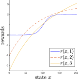
(a) Rewards

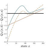
(b) $Q$-function for MDP

Figure 1: Interval Dominant Rewards that are not single crossing and so not supermodular. If supermodularity holds then the curves would be increasing with $x$. Yet $\mathcal{I}$ holds by Corollary 1 and the optimal policy is monotone; see Example (i).

Consider a discounted reward MDP. Assume:

1. For each pair of actions $a,a+1$, assume there is state $x_{a}^{*}$ such that $r(x,a+1)\leq r(x,a)$, $P_{x}(a+1)\leq_{s}P_{x}(a)$ for $x\leq x_{a}^{*}$. Also $r(x,a+1)\geq r(x,a)$, $P_{x}(a+1)\geq_{s}P_{x}(a)$ for $x\geq x_{a}^{*}$.

Corollary 1

Consider a discounted reward MDP. Assume (A1), (A2), (Ex1.1). Then Theorem 1 holds.

Compared to textbook Proposition 1, Statement 1 of Corollary 1 does not impose supermodularity conditions on the rewards or transition probabilities. (Ex1.1) is weaker than the single crossing condition.

Proof: We verify that the conditions (A6), (A7),  (A8) of Theorem 1 hold:

First consider $x<\bar{x}\leq x^{*}_{a}$. Since $r(x,a)\geq r(x,a+1)$, and $r(\bar{x},a)\geq r(\bar{x},a+1)$, (A6) holds for all $\beta\in[\beta^{*}_{x,\bar{x},a},\infty)$ for some $\beta^{*}_{x,\bar{x},a}>0$. Also $P_{x}(a+1)\leq_{s}P_{x}(a)$ implies (A7) holds for all $\alpha_{x,\bar{x},a}\in[\alpha^{*}_{x,\bar{x},a},\infty)$ for some $\alpha^{*}_{x,\bar{x},a}>0$. So we can choose $\alpha=\beta=\max_{a}\{\alpha^{*}_{x,\bar{x},a},\beta^{*}_{x,\bar{x},a}\}$ independent of $a$ so that (A8) holds.

Next consider $\bar{x}>x\geq x^{*}_{a}$. Then (A6) holds for all $\beta\in(0,\beta^{*}_{x,\bar{x},a}]$ for some $\beta^{*}_{x,\bar{x},a}>0$. Also $P_{x}(a+1)\geq_{s}P_{x}(a)$ implies (A7) holds for all $\alpha\in(0,\alpha^{*}_{x,\bar{x},a}]$ for some $\alpha^{*}_{x,\bar{x},a}>0$. Therefore, we can choose $\alpha=\beta=\min_{a}\{\alpha^{*}_{x,\bar{x},a},\beta^{*}_{x,\bar{x},a}\}$ independent of $a$ so that (A8) holds. Finally, for $x\leq x^{*}_{a}$ and $\bar{x}>x^{*}_{a}$, (A6) and (A7) hold for all $\alpha,\beta>0$. So Theorem 1 applies and $\mu^{*}(x)\uparrow x$. $\square$

Example (i). Sigmoidal and Concave Rewards

The following MDP parameters satisfy the assumptions of Corollary 1: $X=201$, $A=3$. The action dependent transition matrices are

$$P_{i}(1)=P_{i-1}(1)+\mu(e_{X}-e_{1}),\quad P_{i}(a+1)=\begin{cases}P_{i}(a)-\epsilon(e_{X}-e_{1}),\;i\leq 50,\\ P_{i}(a)+\epsilon(e_{X}-e_{1}),\;i>50\end{cases}\mu=\frac{0.004}{X},\;\epsilon=\frac{0.05}{X}$$

Here $e_{i}$ denotes the unit $X$-dimension row vector with 1 in the $i$-th position.

The rewards parametrized by $\theta=[2,X-1,20,5,80,-2,5,80,-3.5,0.01]$ are

$$\begin{split}r(x,1)&=\frac{\theta_{1}}{1+\exp(\frac{x-\theta_{2}}{\theta_{3}})},\;r(x,2)=\theta_{4}(1-\exp(-\frac{x}{\theta_{5}}))+\theta_{6},\\ r(x,3)&=\theta_{7}(1-\exp(-\frac{x}{\theta_{8}}))+\theta_{9}+\theta_{10}\,x,\end{split}$$ (12)

Figure 1(b) shows the non-supermodular $Q_{N}$ for $N=100$, $\rho=0.9$. $Q_{N}(x,3)-Q_{N}(x,1)$ (broken line) intersects the horizontal axis three times; so single crossing does not hold. $Q_{N}(x,2)-Q_{N}(x,1)$ (blue line) is non-monotone (non-supermodular). Statement 1, Corollary 1 applies; so the optimal policy is monotone.

Example (ii). Prospect Theory based rewards

In prospect theory (Kahneman and Tversky, 1979), an agent (human decision maker) $a$ has utility $r(x,a)$ that is asymmetric sigmoidal in $x$. This asymmetry reflects a human decision maker’s risk seeking behavior (larger slope) for losses and risk averse behavior (smaller slope) for gains. With $X$ an even integer, the prospect theory rewards are

$$r(x,a)=\frac{2(\mu\,(x-1))^{\theta(a)}}{1+(\mu\,(x-1))^{\theta(a)}}-1,\quad\mu=2/(X-2),\;\theta(a)>1$$ (13)

so they cross zero at $x=X/2$. The shape parameter $\theta(a)$ determines the slope of the reward curve $r(x,a)$.

Suppose the agents (investment managers) range from $a=1$ (cautious) to $a=A$ (aggressive); so the shape parameter $\theta(a)\uparrow a$. The value of an investment evolves according to Markov chain $x_{k}$ with transition probabilities $P(a_{k})$ based on agent $a_{k}$. Since agent $a+1$ is more aggressive (risk seeking) than agent $a$ in losses and gains, it incurs higher volatility. So the $x$-th row of $P(a)$ and $P(a+1)$ satisfy

$$P_{x}(a+1)\leq_{s}P_{x}(a),\;x<X/2\quad\text{ and }P_{x}(a+1)\geq_{s}P_{x}(a),\;x\geq X/2$$ (14)

The aim is to choose the optimal agent $a_{k}$ at each time $k$ to maximize the discounted infinite horizon reward. Since $r(x,a)$ is single crossing but not supermodular, (A3) does not apply.

Corollary 2

Consider a discounted reward MDP with $r(x,a)$ specified by (13) and $\theta(a)\uparrow a$. Assume (A2), (14) hold. Then Theorem 1 holds.

The proof follows from Corollary 1 with $x^{*}_{a}=X/2$.

3.2 Example 2. Interval Dominant Transition Probabilities

Corollary 3

Consider the discounted reward MDP with $r(x,a)=\phi(x)$ where $\phi$ is increasing and non-negative in $x$. Suppose the $i$-th row of transition matrix $P(a)$ is

$$P_{i}(a)=p+\Delta_{i,a}\,(e_{X}-e_{1})$$ (15)

Here $e_{i}$ denotes the unit $X$-dimension row vector with 1 in the $i$-th position. $p$ is an arbitrary $X$-dimensional probability row vector. Also $\Delta_{1,a}=0$, $\Delta_{i,a}\in[0,1]$ are increasing in $i$, and satisfy $\mathcal{I}$  (3). (Also, $\Delta_{i,a}\leq\min\{p_{1},1-p_{X}\}$ to ensure $P(a)$ is valid transition matrix.) Then Theorem 1 holds.

Compared to supermodularity (A4) of the transition probabilities, Corollary 3 imposes weaker conditions: $\Delta$ satisfy $\mathcal{I}$  (3) and $p$ can be any probability vector. Since $\Delta$ only needs to satisfy $\mathcal{I}$ (suitably scaled and shifted to ensure valid probabilities), (15) offers considerable flexibility in choice of the transition matrices.

Proof: Reward $r(x,a)=\phi(x)$ satisfies (A1), (A6) for all $\beta_{x,\bar{x},a}>0$. Also $\Delta_{x,a}\uparrow x$ implies (A2) holds. Next let us verify (A7). Using (15), we need to verify

$$(\Delta_{\bar{x},a+1}-\Delta_{\bar{x},a})\,\sum_{j\geq l}(e_{X}-e_{1})^{\prime}e_{j}\geq\alpha_{x,\bar{x},a}\big{[}(\Delta_{x,a+1}-\Delta_{x,a})\,\sum_{j\geq l}(e_{X}-e_{1})^{\prime}e_{j}\big{]}$$ (16)

where $\alpha_{x,\bar{x},a}>0$ is increasing in $a$. Since $\sum_{j\geq l}(e_{X}-e_{1})^{\prime}e_{j}\geq 0$, clearly $\Delta_{i,a}$ satisfying (3) for some $\alpha_{x,\bar{x},a}>0$ increasing in $a$ is a sufficient condition for (16) to hold. Since the choice of $\beta_{x,\bar{x},a}>0$ is unrestricted, we can choose $\beta_{x,\bar{x},a}=\alpha_{x,\bar{x},a}$. Hence (A8) holds. Thus Theorem 1 holds. $\square$

Example. Suppose $p$ is an arbitrary probability vector, and $\Delta$ is chosen as the rewards (12) suitably scaled and shifted. Then the transition matrices inherit the sigmoidal and concave structures of Sec. 3.1.

3.3 Example 3. Discounted MDP with Perturbed Bi-diagonal Transition Matrices

This section illustrates the $\mathcal{I}$ condition in MDPs with perturbed bi-diagonal transition matrices. The E-companion discusses an example in optimal allocation problems with penalty costs (Ross, 1983; Derman et al., 1976). It also has applications in wireless transmission control (Ngo and Krishnamurthy, 2010).

Consider an infinite horizon discounted reward MDP. The action-dependent transition matrices $P^{\epsilon}(a),a\in\mathcal{A}$ specified by parameter $p_{a}\in[0,1]$ are

$$\begin{split}P^{\epsilon}_{11}(a)&=1-(A-a)\,\epsilon,\quad P^{\epsilon}_{1,X}(a)=(A-a)\,\epsilon,\quad P^{\epsilon}_{X,X-1}(a)=p_{a},\quad P^{\epsilon}_{X,X}(a)=1-p_{a}\\ P^{\epsilon}_{ii}(a)&=1-p_{a}-(A-a)\,\epsilon,\quad P^{\epsilon}_{i,i-1}(a)=p_{a},\quad P^{\epsilon}_{i,X}(a)=(A-a)\epsilon,\quad i=2,\ldots,X-1\end{split}$$ (17)

where $\epsilon\ll 1$ is a small positive real. We assume that $p_{a}$ is increasing in $a$. When $\epsilon=0$, $P^{\epsilon}(a)$ are bi-diagonal transition matrices; so $\epsilon$ can be viewed as a perturbation probability of a bi-diagonal transition matrix.

Supermodularity (A4) of the transition matrices (17) holds if $\epsilon\geq p_{a+1}-p_{a}$. In this section we assume $\epsilon$ is a small parameter with $\epsilon\leq\min_{a}p_{a+1}-p_{a}$, so that (A4) does not hold. Therefore, textbook Proposition 1 does not hold. We show how the $\mathcal{I}$ condition and Theorem 1 apply.

Remark. In our result below, to show condition $\mathcal{I}$ holds, we choose $\alpha_{a}=\beta_{a}=(p_{a+1}-p_{a})/\epsilon=\gamma_{a}$. If $p_{a}$ is differentiable wrt $a$, then as $\epsilon\rightarrow 0$, i.e., for an MDP with bi-diagonal transition matrices, this can be interpreted as choosing $\alpha_{a}=\beta_{a}=dp_{a}/da$.

Corollary 4

Consider a discounted cost MDP with transition probabilities (17). Assume $p_{a}$ is increasing in $a$ and $p_{a+1}-p_{a}=\gamma_{a}\epsilon$ for some positive real number $\gamma_{a}$ increasing in $a$. Assume (A1) and that

$$r(i+1,a+1)-r(i+1,a)\geq\beta_{a}\,[r(i,a+1)-r(i,a)]$$ (18)

for some $\beta_{a}$ increasing in $a$ with $\beta_{a}\geq\gamma_{a}$. Then optimal policy $\mu^{*}(x)\uparrow x$.

Proof: We verify that the assumptions in Theorem 1 hold. (A1) holds by assumption. From the structure of $P^{\epsilon}(a)$ in (17) it is clear that (A2) holds. Considering actions $a$ and $a+1$, it is verified that (A7) holds for all $\alpha_{a}\geq(p_{a+1}-p_{a})/\epsilon=\gamma_{a}$. Next by assumption (18), (A6) holds for $\beta_{a}\geq\gamma_{a}$. Finally, we can choose $\alpha_{a}=\beta_{a}\geq\gamma_{a}$, and so (A8) holds. $\square$

Example. $A=2,X=6$, $p_{1}=0.3$, $p_{2}=p_{1}+20\epsilon$, $\epsilon=10^{-3}$, $\rho=0.9$, $N=200$, $r^{\prime}=\begin{bmatrix}1&3.5&6&6&11&43\\ 0&2&3&6&12&63\end{bmatrix}$. Given the transition probabilities, we choose $\alpha\geq 20$. Also for the rewards, we choose $\beta=20$ in (18). So Corollary 4 holds. Figure 2 shows $Q_{N}(x,a)$ is not supermodular, yet the optimal policy is monotone with $\mu^{*}(i)=1$ for $i\in\{1,2,3,4\}$ and $\mu^{*}(i)=2$ for $i\in\{5,6\}$.

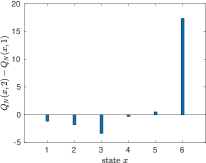
Figure 2: The $Q$-function is not-supermodular for an MDP with perturbed bi-diagonal matrices; yet the optimal policy $\mu^{*}(x)$ is increasing in state $x$ by Corollary 4.

4 Example 4. MDPs with Concave Value Functions

Theorem 1 used first order dominance and monotone costs to establish $\mathcal{I}$ and therefore monotone optimal policies. In comparison, this section extends Theorem 1 to MDPs where the value function is concave. We use second order stochastic dominance and concave costs to establish $\mathcal{I}$ and therefore monotone optimal policies. The results below assume a TP3 transition matrix; see Karlin (1968) for the rich structure involving their diminishing variation property. For convenience we minimize costs instead of maximize rewards.

1. Costs $c(x,a)$ are increasing and concave in $x$ for each $a$.

2. $P(a)$ is TP3with $\sum_{j=1}^{X}jP_{ij}(a)$ increasing and concave in $i$. Totally positive of order 3 means that each 3rd order minor of $P(a)$ is non-negative.

3. For $\beta_{x,\bar{x},a}>0$ and increasing in $a$, $c(\bar{x},a+1)-c(\bar{x},a)\geq\beta_{x,\bar{x},a}\,\big{[}c(x,a+1)-c(x,a)\big{]},\quad\bar{x}>x$.

4. For $\alpha_{x,\bar{x},a}>0$ and increasing in $a$, $\frac{P_{\bar{x}}(a+1)+\alpha_{x,\bar{x},a}\,P_{x}(a)}{1+\alpha_{x,\bar{x},a}}>_{2}\frac{P_{\bar{x}}(a)+\alpha_{x,\bar{x},a}\,P_{x}(a+1)}{1+\alpha_{x,\bar{x},a}},\quad\bar{x}>x$ where $>_{2}$ denotes second order stochastic dominance.

5. Terminal cost ${\tau}_{x}$ is increasing and concave in $x$.

Remarks. (i) As shown in the proof, (C1) (concavity), (C2), (C5) imply the value function is concave and increasing. These together with (C3), (C4) and (A8) imply $\mathcal{I}$ holds and so the optimal policy is monotone.

(ii) (C2) generalizes the assumption that $\sum_{j}j{P}_{ij}$ is linear increasing in $i$. The classical result in Karlin (1968, pg 23) states: Suppose $P$ is a TP3 transition matrix and $\sum_{j}j{P}_{ij}$ is linear increasing in $i$. If vector $V$ is concave, then vector $P\,V$ is concave. However, for bi-diagonal and tri-diagonal transition matrices, $\sum_{j}jP_{ij}$ is concave (or convex) and not linear in $i$ (see examples below). This is why we introduced (C2). Since the classical result requires $\sum_{j}j{P}_{ij}$ being linear in $i$, it no longer applies. So we will prove a small generalization that handles the case where $\sum_{j}jP_{ij}$ is concave in $i$ (see Lemma 1 below).

Theorem 2

(i) For a discounted cost MDP under (C1)-(C4), (A8), optimal policy $\mu^{*}(x)\downarrow x$.
(ii) For a finite horizon MDP, under (C1)-(C5), (A8), optimal policy sequence $\mu^{*}_{k}(x)$, $k=0,\ldots,N$ $\downarrow x$.

Corollary 5

Consider the modified assumptions: (C1): increasing replaced by decreasing; (C2) concave replaced with convex; (C3): inequality involving costs reversed; (C4): $>_{2}$ replaced by convex dominance $>_{c}$; (C5): increasing replaced by decreasing. Under these assumptions and (A8), Theorem 2 holds with the modification $\mu^{*}(x)$ and $\mu^{*}_{k}(x)$, are increasing in $x$.

Proof: (Theorem 2) We prove statement (ii). The proof of statement (i) is similar and omitted.

First we show by induction that $V_{k}(i)$ is increasing in $i$ for $k=N,\ldots,1$. By (C5), $V_{N}(i)={\tau}_{i}$ is increasing. Assume $V_{k+1}(i)$ is increasing in $i$. TP3 assumption (C2) implies TP2 which preserves monotone functions (Karlin, 1968, pg 23), (Lehmann and Casella, 1998), namely, $\sum_{j}P_{ij}(a)V_{k+1}(j)$ is increasing in $i$. This together with (C1) implies $Q_{k}(i,a)$ is increasing. Thus $V_{k}(i)=\min_{a}Q_{k}(i,a)$ is increasing in $i$.

Next we show by induction that $V_{k}(i)$ is concave in $i$. By (C5), $V_{N}={\tau}$ is concave. Assume $V_{k+1}$ is concave. Then (C2) implies $\sum_{j}P_{ij}(a)\,V_{k+1}(j)$ is concave in $i$ (see Lemma 1 below). Since $c(i,a)$ is concave by (C1), it follows that $Q_{k}(i,a)=c(i,a)+\sum_{j}P_{ij}(a)\,V_{k+1}(j)$ is concave in $i$. Since concavity is preserved by minimization, $V_{k}(i)=\min_{a}Q_{k}(i,a)$ is concave. Finally, $V_{k}(i)$ increasing and concave in $i$ and (C4) implies (10) holds for all $\alpha_{x,\bar{x},a}\geq 1$. Then with (C3),(A8), the proof is identical to (11) in Theorem 1. $\square$

The following lemma used in the proof of Theorem 2 slightly extends the result in Karlin (1968, pg 23).

Lemma 1

Suppose $P$ satisfies (C2). If $V$ is concave and increasing, then $P\,V$ is concave and increasing.

Proof: First TP3 preserves monotonicity, so $PV$ is increasing. Next, since $V$ is concave and increasing, then for any $a>0$ and $b\in\mathbb{R}$, $V(j)-(aj+b)$ has two or fewer sign changes in the order $-,+,-$ as $j$ increases from 1 to $X$. Let $\phi_{i}(a,b)=\sum_{j}P_{ij}(aj+b)$. Since $P$ is TP3, the diminishing variation property of TP3 implies $\sum_{j}P_{ij}\,V_{j}-\phi_{i}(a,b)$ also has two or fewer sign changes in the order $-,+,-$ as $i$ increases from 1 to $X$. Assume two sign changes occur; then for some $i_{1}<i_{2}$, $\sum_{j}P_{ij}\,V_{j}\geq\phi_{i}(a,b)$ for $i_{1}\leq i\leq i_{2}$. Since $\phi_{i}(a,b)$ is integer concave in $i$ by (C2), it lies above the line segment $L_{i}$ that connects $(i_{1},\phi_{i_{1}})$ to $(i_{2},\phi_{i_{2}})$. So $\sum_{j}P_{ij}\,V_{j}\geq\phi_{i}(a,b)\geq L_{i}$, $i_{1}\leq i\leq i_{2}$ Finally, for arbitrary $i_{1}<i_{2}\in\{1,\ldots,X\}$, we can choose $a=\frac{\sum_{j}V_{j}(P_{i_{2},j}-P_{i_{1},j})}{\sum_{j}j(P_{i_{2},j}-P_{i_{1},j})}$ and $b=\sum_{j}P_{i_{1},j}V_{j}-a\sum_{j}j\,P_{i_{1},j}$ so that $\sum_{j}P_{ij}\,V_{j}=\phi_{i}(a,b)=L_{i}$ at $i=i_{1},i_{2}$. Clearly, $\sum_{j}P_{ij}\,V_{j}\geq L_{i}$ for arbitrary $i_{1}\leq i\leq i_{2}$ and $\sum_{j}P_{ij}\,V_{j}=L_{i}$ for $i=i_{1},i_{2}$ implies $\sum_{j}P_{ij}\,V(j)$ is concave. $\square$

Example (i). Bi-diagonal Transition Matrices and Non-supermodular Costs

Theorem 2 applies to bi-diagonal transition matrices with possibly non-supermodular costs; this is in contrast to Sec. 3.3 where we considered perturbed bi-diagonal matrices. Consider an MDP with bi-diagonal transition matrices $P_{i.i}(a)=1-p_{a},\;P_{1,i+1}=p_{a},\;P_{X,X}(a)=1,\quad a\in\{1,\ldots,A\}$. Then $\sum_{j}jP_{ij}(a)=i+p_{a}$ for $i<X$ and $X$ for $i=X$; so $\sum_{j}jP_{ij}(a)$ is increasing and concave in $i$ ((C2) holds). Assume $p_{a}\downarrow a$. Then (C4) is equivalent to $\sum_{\l\leq m}\sum_{j\leq l}P_{\bar{x},j}(a+1)-P_{\bar{x},j}(a)\leq\alpha_{x,\bar{x},a}(\sum_{\l\leq m}\sum_{j\leq l}P_{x,j}(a+1)-P_{x,j}(a))$. Since $p_{a}\geq p_{a+1}$, it follows that  (C4) holds for all $\alpha_{x,\bar{x},a}\geq 1$. If (C1), (C3) hold for some $\beta_{x,\bar{x},a}>1$, then Theorem 2 holds.

Remarks. (i) For $A=2$, and concave increasing costs $c(x,1),c(x,2)$, the following useful single crossing characterization satisfies (C3). Suppose $c(x=1,2)<c(x=1,1)$ and the curves $c(x,2)$ and $c(x,1)$ intersect once at $x^{*}$. For $x\geq x^{*}$, the curve $c(x,2)$ grows faster than $c(x,1)$, i.e., $c(x,a)$ is supermodular for $x\geq x^{*}$. For $x<x^{*}$, the difference between $c(x,1)$ and $c(x,2)$ can be arbitrary. Figure 3(i) illustrates this.
(ii) To motivate Theorem 2, (A4) does not hold for bi-diagonal matrices. Since $\beta>1$, supermodularity (A3) does not hold. Also, Theorem 1 does not apply since (A7) does not hold.

Numerical example. Consider a discounted cost MDP with $A=2$, $X=50$, $p_{1}=0.8$, $p_{2}=0.7$, $\rho=0.95$, $N=200$, $c(x,1)=\theta_{1}x^{2}+\theta_{2}x+\theta_{3},\quad c(x,2)=\theta_{4}\big{(}1-\exp(\theta_{5}x+\theta_{6})\big{)}$, $\theta=[-0.01,1,8.8,25,-0.1,-0.4]$. It can be verified that the cost is not supermodular, but the conditions of Theorem 2 are satisfied. So the value function is concave and optimal policy is decreasing. Figure 3(ii) shows $Q_{N}(x,a)$ is not submodular.

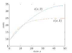
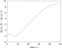
Figure 3: Concave costs and non-submodular $Q$ function for MDP with bi-diagonal transition matrix that satisfies Theorem 2.

Example (ii). Tri-diagonal Transition Matrices and Non-submodular Costs

Corollary 5 applies to MDPs with tri-diagonal transition matrices where $P_{i-1,i}(a)=p_{a},\;P_{i+1,i}=q_{a},\;P_{ii}=1-p_{a}-q_{a},\;P_{11}(a)=1,\;P_{X-1,X}=1-s_{a},P_{X,X}=s_{a}$. If $P(a)$ is TP3 and $q_{a}<p_{a}$, $s_{a}>1+q_{a}-p_{a}$ hold, then $\sum_{i}jP_{ij}(a)$ is increasing and convex in $i$; so modified (C2) holds. Also, if $q_{a}\uparrow a$, $p_{a}\downarrow a$, $q_{a+1}-q_{a}\geq p_{a+1}-p_{a}$, $s_{a+1}-s_{a}>q_{a+1}-q_{a}+p_{a}-p_{a+1}$, then convex dominance (modified (C4)) holds for all $\alpha\in(0,1]$. Then if the costs are chosen so that modified (C1), and modified (C3) hold for some $\beta_{x,\bar{x},a}\leq 1$, then Corollary 5 holds and the optimal policy is monotone (even though the costs are not submodular when $\beta<1$).

Numerical example. Consider a discounted cost MDP with $A=2$, $X=35$, tri-diagonal transition matrices with $p_{1}=0.2,p_{2}=0.1,q_{1}=0.05,q_{2}=0.1,s_{1}=0.95,s_{2}=1$. Also $\rho=0.95$, $N=200$, $c(x,1)=-(\theta_{1}+\theta_{2}\,x^{3}),\quad c(x,2)=-(\theta_{3}+\theta_{4}x^{3})$ where $\theta=[15,0.3/4^{3},1,3/4^{3}]$. The cost $c(x,a)$ is not submodular (see Figure 4(i)), but Corollary 5 holds. Figure 4(ii) shows the non-submodular $Q_{N}(x,a)$.

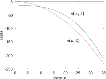
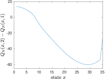
Figure 4: Non-submodular concave costs and non-submodular $Q$ function for MDP with tri-diagonal transition matrix that satisfies Corollary 5.

5 Summary and Discussion

Summary. The textbook structural result for MDPs uses supermodularity to establish the existence of monotone optimal policies. This paper shows how supermodularity can be relaxed by formulating a sufficient condition for interval dominance, which we call the $\mathcal{I}$ condition. We presented several examples of MDPs which satisfy $\mathcal{I}$ including sigmoidal costs, and bi-diagonal/perturbed bi-diagonal transition matrices. The structural results in Sec.3, namely, Theorem 1, Corollaries 1, 3, 4 and Theorem 3 used first order stochastic dominance to establish $\mathcal{I}$ for several examples. of MDPs. In comparison, Theorem 2 in Sec.4 discussed examples of $\mathcal{I}$ in MDPs with concave value functions; we used TP3 assumptions and second order (convex) stochastic dominance to prove the existence of monotone optimal policies.

Discussion 1. Reinforcement Learning (RL) and Differential sparse Policies: Once the existence of a monotone optimal policy has been established, RL algorithms that exploit this structure can be constructed. Q-learning algorithms that exploit the $\mathcal{I}$ condition can be obtained by generalizing the supermodular Q-learning algorithms in Krishnamurthy (2016). The second approach is to develop policy search RL algorithms. In particular, when $A$ is small and $X$ is large, then since $\mu^{*}(x)\uparrow x$, it is differentially sparse, that is $\mu^{*}(x+1)-\mu^{*}(x)$ is positive only at $A-1$ values of $x$, and zero for all other $x$. In Mattila et al. (2017), LASSO based methods are developed to exploit this sparsity and significantly accelerate search for $\mu^{*}(x)$; they build on the nearly-isotonic regression techniques in Tibshirani et al. (2011). The idea is to add a rectified $l_{1}$-penalty $\sum_{x=1}^{X-1}|\mu^{l}(x)-\mu^{l}(x+1)|_{+}$ to the cost in the optimization problem (here $\mu^{l}$ is the estimate of the optimal policy at iteration $l$ of the optimization algorithm). Intuitively, this modifies the cost surface to be more steep in the direction of monotone policies resulting in faster convergence of an iterative optimization algorithm.

Discussion 2. Convex Value Functions: Can Theorem 2 be extended to MDPs with convex value functions? Since convexity is not preserved by minimization, we need multimodularity assumptions to show the value function is convex. However, since multimodularity implies supermodularity, we are unable to exploit the weaker $\mathcal{I}$ condition. Multimodularity is sufficient (but not necessary) for convexity to be preserved by minimization; so it is worthwhile exploring relaxed $\mathcal{I}$ based versions that do not require supermodularity.

Appendix A Toy Example Illustrating $\mathcal{I}$ Rewards

Sec. 3.1 discussed an intuitive visualization of $\mathcal{I}$ property of rewards for a MDP in terms of the reward curves vs state. We now provide a second intuitive visualization displayed in Figure 5(a) in terms of the reward curves vs actions $a$. This is similar to the discussion in Quah and Strulovici [2009]. For supermodular rewards, $r(3,a)-r(2,a)$ increases with $a$. Examining Figure 5(a), for $a\leq a_{x}$ (where $a_{x}=\operatornamewithlimits{arg\,max}_{a}r(x,a)=2$), the differences between the reward curves can be arbitrary, as long as $r(3,a)\geq r(2,a)$ as required by (A1). Also the $r(3,a)$ curve satisfies that $r(3,1)>r(3,3)$, while the $r(2,a)$ curve satisfies $r(2,1)<r(2,3)$; so the single crossing property is violated. Yet condition $\mathcal{I}$ , namely,  (A6) holds.

The following MDP satisfies Theorem 1: $\rho=0.9$, $X=4$, $A=3$, $N=100$,

$$r=\begin{bmatrix}12&4&0\\ 16&22&18\\ 22&23&20\\ 24&28&30\end{bmatrix},P(1)=\begin{bmatrix}0.3&0.4&0.2&0.1\\ 0.2&0.4&0.2&0.2\\ 0.2&0.4&0.1&0.3\\ 0.2&0.3&0.1&0.4\end{bmatrix},P(2)=\begin{bmatrix}0.3&0.3&0.2&0.2\\ 0.2&0.3&0.2&0.3\\ 0.2&0.3&0.1&0.4\\ 0.2&0.2&0.1&0.5\end{bmatrix},P(3)=\begin{bmatrix}0.3&0.3&0.1&0.3\\ 0.2&0.3&0.1&0.4\\ 0.2&0.2&0.1&0.5\\ 0.1&0.2&0.1&0.6\end{bmatrix}$$

Note that $r(2,3)-r(2,1)>0$ while $r(3,3)-r(3,1)<0$. Jointly, these violate both supermodularity and also single crossing. But the $\mathcal{I}$ condition (3) holds since it compares action 1 with action 2, and action 2 with action 3. Indeed, (A6) holds for $\beta_{a=1}\leq 1/6$ and $\beta_{a=2}=1$. Also (A7) holds for all $\alpha\leq 1$. Figure 5(b) plots $Q_{100}(x,2)-Q_{100}(x,1)$ and $Q_{100}(x,3)-Q_{100}(x,1)$. Clearly $Q_{k}(x,a)$ is not supermodular. But the optimal policy is monotone by Theorem 1.

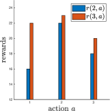
(a) Non-single crossing reward

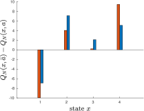
(b) Non-single crossing $Q$ function

Figure 5: MDP with $X=4,A=3$. If supermodularity holds then the bars would be increasing with $x$. Yet $\mathcal{I}$ holds by Corollary 1 and the optimal policy is monotone.

Appendix B Optimal Allocation MDP with Penalty Cost

This section discusses a finite horizon penalty-cost MDP with perturbed bi-diagonal transition matrices (17). This has applications in optimal allocation problems with penalty costs [Ross, 1983, Derman et al., 1976] and wireless transmission control [Ngo and Krishnamurthy, 2010]. We assume $\epsilon<p_{a+1}-p_{a}$; so as discussed in Sec. 3.3 supermodularity condition (A4) does not hold.

As in Example 4.2 in Ross [1983, pg.8] and Derman et al. [1976], we consider an $N$-horizon MDP model. There are $N$-stages to construct $X$ components sequentially. If effort $c(x,a)$ is allocated then the component is constructed with successfully with probability $p_{a}$. Our transition matrices are specified by the perturbed bi-diagonal matrices (17). At the end of $N$ stages, the penalty cost incurred is ${\tau}_{i}$ if we are $i$ components short, where $i=\{1,\ldots,X\}$, with ${\tau}_{1}=0$. Ross [1983] considers a continuous action space as the closed interval $\mathcal{A}=[0,A]$, $c(x,a)=a$ where $a\in\mathcal{A}$ and bi-diagonal matrices ($\epsilon=0$). Although the $\mathcal{I}$ condition yields degenerate policies for $c(x,a)=a$, it applies to non-supermodular cost structures with perturbed bi-diagonal matrices. Such cases cannot be handled by the convexity based supermodularity approach.

We consider the discrete action space $\mathcal{A}=\{1,\ldots,A\}$ corresponding to discretization of the continuous valued actions: $\bar{\mathcal{A}}=\{0,\;\epsilon,\;2\,\epsilon,\ldots,(A-1)\,\epsilon\}$. Recall $\epsilon$ are perturbation probabilities of the bi-diagonal transition matrices in (17). The costs and transition probability parameter $p_{a}$ in terms of the discretized actions are

$$\text{ Costs: }c(x,a)\,\epsilon,\quad p_{a+1}-p_{a}=\epsilon\,\gamma_{a}\;\;\text{ where }\gamma_{a}>0.$$ (19)

We make the following assumptions; they are discussed after Theorem 3 below.

1. $\gamma_{a}\geq 1$ and $\uparrow a$. (The $\uparrow a$ can be relaxed, see remark below.)

2. Terminal cost ${\tau}_{x}$ convex and $\uparrow x$ with ${\tau}_{1}=0$. Cost $c(x,a)\downarrow x$. (More generally, $\bar{c}(x,a)$ in (20) $\downarrow x$.)

Main Result. We will work with the modified value function $W_{k}(x)=V^{\epsilon}_{k}(x)-{\tau}_{x}$. This is convenient since the terminal condition is $W_{N}(i)=0$ for all $i$. The dynamic programming recursion (6) expressed in terms of $W_{k}(x)$ and minimizing the cumulative cost (rather than maximizing the cumulative reward) is

$$\mu^{*}_{k}(x) =\operatornamewithlimits{arg\,min}_{a}\bar{Q}_{k}(x,a),\quad W_{k}(x)=\min_{a}\bar{Q}_{k}(x,a),\quad k=0,\ldots,N-1$$

$$\bar{Q}_{k}(i,a) =\bar{c}(i,a)+\big{(}1-p_{a}-\epsilon(A-a)\big{)}\,W_{k+1}(i)+p_{a}W_{k+1}(i-1)$$

where $$\quad\bar{c}(i,a)=\epsilon\,c(i,a)+p_{a}\,({\tau}_{i-1}-{\tau}_{i})+\epsilon\,(A-a)\,({\tau}_{X}-{\tau}_{i}),\quad i=1,\ldots,X-1$$ (20)

$$\bar{Q}_{k}(X,a)=\bar{c}(X,a)+p_{a}W_{k+1}(X-1)+(1-p_{a})\,W_{k+1}(X),\;\bar{c}(X,a)=\epsilon\,c(X,a)+p_{a}({\tau}_{X-1}-{\tau}_{X})$$

Theorem 3

Consider the $N$-horizon MDP with costs and transition probabilities specified by (19), (17). Assume (A9) and (A10). Suppose $\min_{a}\gamma_{a}>1$ and the costs satisfy

$${\tau}_{i+1}\geq{\tau}_{X}+\frac{\gamma_{a}^{2}\,({\tau}_{i}-{\tau}_{i-1})}{\gamma_{a}-1}+\frac{\Delta(i+1,a)-\gamma_{a}\Delta(i,a)}{\gamma_{a}-1},\quad i=2,\ldots,X-1$$ (21)

where $\Delta(i,a)=c(i,a+1)-c(i,a)$ and perturbation probabilities $\epsilon\in\big{(}0,\min_{a}(p_{a+1}-p_{a})\big{)}$. Then optimal policy $\mu^{*}_{k}(i)$, $k=1,\ldots,N-1$, is increasing in state $i$.

Remarks. 1. Theorem 3 can be viewed as complementary result to the structural result in Ross [1983], Derman et al. [1976]. On the one hand, if we choose the same instantaneous cost as Ross [1983], namely $c(x,a)=f\,a$ for some constant $f$, then (21) becomes ${\tau}_{i+1}\geq{\tau}_{X}+\frac{\gamma_{a}^{2}\,({\tau}_{i}-{\tau}_{i-1})}{\gamma_{a}-1}-f$. But terminal costs satisfying this condition yield monotone policies that are degenerate, namely, $\mu^{*}_{k}(i)=1$ for all $i$. So for $c(x,a)=f\,a$, the $\mathcal{I}$ condition does not yield a useful result. It is necessary to exploit convexity of the value function, as in Ross [1983], to obtain non-degenerate optimal policies.

On the other hand, the $\mathcal{I}$ condition (21) allows for non-submodular costs and yields monotone policies (see examples below). For such cases, it is not clear how to extend the convexity based submodularity proof in  Ross [1983] (which applies when $\epsilon=0$) to the MDP (17) for arbitrary $\epsilon>0$.
2. Regarding the assumptions, (A9) is equivalent to $p_{a}\uparrow a$ and convex. (A9) can be relaxed to $p_{a}\uparrow a$ by imposing stronger conditions on (21), see (22) below. The convexity (A10) of terminal costs implies $\bar{c}(i,a)$ in (20) is decreasing. Recall decreasing costs (A1) is used to show submodularity (and Theorem 1).
3. Theorem 3 considers costs (negative of rewards) whereas Theorem 1 considers rewards. Note (A1) is equivalent to the cost decreasing in the state. Also inequality (A6) is reversed in terms of costs.

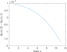
(a) $Q$ function for submodular cost

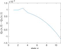
(b) $Q$ function for non-submodular cost

Figure 6: $Q$ function for Optimal Allocation MDP

Examples. We chose the MDP parameters in (17), (19) as $X=11$, $A=2$, $\gamma_{a}=1.2$, $\epsilon=10^{-6}$, ${\tau}=[0,1,2,4,8,15,25,40,60,90,200]$. Figure 6 displays $Q_{k}(x,2)-Q_{k}(x,1)$ for two cases: (i) $c(x,1)=0$, $c(x,2)=\epsilon(f-(x+2)^{3})$, $f=10^{3}$ (ii) $c(x,1)=0$, $c(x,2)=\epsilon(f+2.5\,x^{4}I(x\leq 3)-(x+2)^{3})$, $f=10^{3}$.
In case (ii), $Q(x,a)$ is not submodular; see Figure 6(b). But Theorem 3 holds; so optimal policy $\mu_{k}^{*}(x)\uparrow x$.

Proof of Theorem 3 Using the modified dynamic programming recursion (20), we verify the assumptions in Theorem 1. Examining the transformed cost $\bar{c}(x,a)$ in (20), (A1) holds for $\bar{c}(x,a)$, $x\in\{1,\ldots,X\}$, if ${\tau}_{i}$ is convex and increasing, and $c(i,a)$ is decreasing in $i$, i.e, (A10) holds. From the structure of $P^{\epsilon}(a)$ in (17), (A2) holds. The terminal cost in  (20) is $0$ for all states; so (A5) holds trivially. Next by (A9), ${d}_{a}>0$. So for actions $a$ and $a+1$, it is easily verified that (A7) holds for $\alpha_{a}\geq{d}_{a}/\epsilon>1$. So $\epsilon\in(0,\min_{a}{d}_{a}]$.

We now establish (A6) for $\bar{c}(x,a)$, $x\in\{1,\ldots,X-1\}$. Choose $\beta_{a}=\alpha_{a}={d}_{a}/\epsilon=\gamma_{a}$ (substituting (19) for ${d}_{a}$). By (A9), $\alpha_{a}>0\uparrow a$. Then (A6) is equivalent to $\epsilon(c(x+1,a+1)-c(x+1,a))+\epsilon\,\gamma_{a}\,({\tau}_{x}-{\tau}_{x+1})+\epsilon\,({\tau}_{x+1}-{\tau}_{X})\leq\beta_{a}\,[\epsilon(c(x,a+1)-c(x,a))+\epsilon\,\gamma_{a}\,({\tau}_{x-1}-{\tau}_{x})+\epsilon\,({\tau}_{x}-{\tau}_{X})]$. The positive parameter $\epsilon$ cancels on both sides, yielding (21). Since $\beta_{a}=\alpha_{a}$, (A8) holds. Thus all conditions of Theorem 1 hold.

Remark. Choosing $\alpha=\bar{\gamma}=\max_{a}\gamma_{a}$ in the proof, we obtain a stronger sufficient condition than (21):

$${\tau}_{i+1}\geq{\tau}_{X}\frac{\bar{\gamma}-1}{\gamma_{a}-1}+\frac{\bar{\gamma}\,\gamma_{a}\,({\tau}_{i}-{\tau}_{i-1})}{\gamma_{a}-1}+\frac{\Delta(i+1,a)-\bar{\gamma}\Delta(i,a)}{\gamma_{a}-1}+\frac{(\gamma_{a}-\bar{\gamma}){\tau}_{i}missing}{\gamma_{a}-1}$$ (22)

Since $\alpha=\beta$ is a constant and not $a$ dependent,  (A9) is relaxed to $\gamma_{a}>1$.

References

- Amir [2005] R. Amir. Supermodularity and complementarity in economics: An elementary survey. Southern Economic Journal, 71(3):636–660, 2005.
- Derman et al. [1976] C. Derman, G. J. Lieberman, and S. M. Ross. Optimal system allocations with penalty cost. Management Science, 23(4):399–403, December 1976.
- Heyman and Sobel [1984] D. P. Heyman and M. J. Sobel. Stochastic Models in Operations Research, volume 2. McGraw-Hill, 1984.
- Kahneman and Tversky [1979] D. Kahneman and A. Tversky. Prospect theory: An analysis of decision under risk. Econometrica, 47(2):263–291, 1979.
- Karlin [1968] S. Karlin. Total Positivity, volume 1. Stanford Univ., 1968.
- Krishnamurthy [2016] V. Krishnamurthy. Partially Observed Markov Decision Processes. From Filtering to Controlled Sensing. Cambridge University Press, 2016.
- Lehmann and Casella [1998] E. Lehmann and G. Casella. Theory of Point Estimation. Springer-Verlag, 2nd edition, 1998.
- Mattila et al. [2017] R. Mattila, C. R. Rojas, V. Krishnamurthy, and B. Wahlberg. Computing monotone policies for markov decision processes: a nearly-isotonic penalty approach. IFAC-PapersOnLine, 50(1):8429–8434, 2017.
- Milgrom and Shannon [1994] P. Milgrom and C. Shannon. Monotone comparative statics. Econometrica, 62(1):157–180, 1994.
- Ngo and Krishnamurthy [2010] M. H. Ngo and V. Krishnamurthy. Monotonicity of constrained optimal transmission policies in correlated fading channels with ARQ. IEEE Transactions on Signal Processing, 58(1):438–451, 2010.
- Puterman [1994] M. Puterman. Markov Decision Processes. John Wiley, 1994.
- Quah and Strulovici [2009] J. Quah and B. Strulovici. Comparative statics, informativeness, and the interval dominance order. Econometrica, 77(6):1949–1992, 2009.
- Ross [1983] S. Ross. Introduction to Stochastic Dynamic Programming. Academic Press, San Diego, California., 1983.
- Tibshirani et al. [2011] R. J. Tibshirani, H. Hoefling, and R. Tibshirani. Nearly-isotonic regression. Technometrics, 53(1):54–61, 2011.
- Topkis [1998] D. M. Topkis. Supermodularity and Complementarity. Princeton University Press, 1998.