The miniJPAS survey: White dwarf science with 56 optical filters

Abstract

Aims. We analyze the white dwarf population in miniJPAS, the first square degree observed with $56$ medium-band, $145\ \AA$ in width optical filters by the Javalambre Physics of the accelerating Universe Astrophysical Survey (J-PAS), to provide a data-based forecast for the white dwarf science with low-resolution ($R\sim 50$) photo-spectra.

Methods. We define the sample of the bluest point-like sources in miniJPAS with $r<21.5$ mag, point-like probability larger than $0.5$, $(u-r)<0.80$ mag, and $(g-i)<0.25$ mag. This sample comprises $33$ sources with spectroscopic information, $11$ white dwarfs and $22$ QSOs. We estimate the effective temperature ($T_{\rm eff}$), the surface gravity, and the composition of the white dwarf population by a Bayesian fitting to the observed photo-spectra.

Results. The miniJPAS data permit the classification of the observed white dwarfs into H-dominated and He-dominated with 99% confidence, and the detection of calcium absorption and polluting metals down to $r\sim 21.5$ mag at least for sources with $7\,000<T_{\rm eff}<22\,000$ K, the temperature range covered by the white dwarfs in miniJPAS. The effective temperature is estimated with a $2$% uncertainty, close to the $1$% from spectroscopy. A precise estimation of the surface gravity depends on the available parallax information. In addition, the white dwarf population at $T_{\rm eff}>7\,000$ K can be segregated from the bluest extragalactic QSOs, providing a clean sample based on optical photometry alone.

Conclusions. The J-PAS low-resolution photo-spectra provide precise and accurate effective temperatures and atmospheric compositions for white dwarfs, complementing the data from Gaia. J-PAS will also detect and characterize new white dwarfs beyond the Gaia magnitude limit, providing faint candidates for spectroscopic follow up.

1 Introduction

White dwarfs are the degenerate remnant of stars with masses lower than $8-10$ $M_{\odot}$ and the endpoint of the stellar evolution for more than 97% of stars (e.g., Ibeling & Heger 2013; Doherty et al. 2015, and references therein). This makes them an essential tool to disentangle the star formation history of the Milky Way, the late phases of stellar evolution, and to understand the physics of condensed matter.

White dwarfs can be selected from the general stellar population thanks to their location in the Hertzsprung-Russell (H-R) diagram, typically being ten magnitudes fainter than main sequence stars of the same effective temperature. The pioneering analysis by Russell (1914) and Hertzsprung (1915) shows only one faint A-type star, $40$ Eri B, with the inclusion of Sirius B (Adams 1915) and van Maanen 2 (van Maanen 1917, 1920) in the lower left hand corner of the H-R diagram by the end of that decade. The initial doubts about the high density derived for these objects were clarified during the next years thanks to the estimation of the gravitational redshift of Sirius B (Adams 1925) and the proposal of electron degeneracy pressure as a counterbalance for the gravitational collapse caused by such condensed matter (Fowler 1926). Once established as an astrophysical object (see Holberg 2009, for a detailed review), the systematic analysis of the white dwarf population begun.

The use of the H-R diagram to search for new white dwarfs was limited by the difficulties in the estimation of precise parallaxes, which are needed to obtain the luminosity of the objects. Because of this, the definition of photometric white dwarf catalogs was mainly based on the search of ultraviolet-excess objects, such as the Palomar-Green catalog (PG, Green et al. 1986), the Kiso survey (KUV, Noguchi et al. 1980; Kondo et al. 1984), or the Kitt Peak-Downes survey (KPD, Downes 1986); and using reduced proper motions (e.g., Luyten 1979; Harris et al. 2006; Rowell & Hambly 2011; Gentile Fusillo et al. 2015; Munn et al. 2017). The spectroscopic follow up of these photometric catalogs revealed a diversity of white dwarf atmospheric compositions (Sion et al. 1983; Wesemael et al. 1993), with sources presenting hydrogen lines (DA type), He II lines (DO), He I lines (DB), metal lines (DZ), and featureless spectra (DC) among others. By the end of the XXth century, about $\sim 3\,000$ white dwarfs with spectroscopic information and only $\sim 300$ with precise parallax measurements were discovered (McCook & Sion 1999).

This difference further increased by one order of magnitude mainly thanks to the spectroscopy from the Sloan Digital Sky Survey (SDSS, York et al. 2000). During almost $20$ years of observations, the different SDSS data releases increased above $20\,000$ the number of white dwarfs with spectroscopic information (Kleinman et al. 2004; Eisenstein et al. 2006; Kepler et al. 2015, 2016, 2019). At the same time, the absolute number of white dwarfs with precise parallaxes did not increase significantly (e.g., Leggett et al. 2018).

The high-quality data from the Gaia mission (Gaia Collaboration et al. 2016) turned around the situation. Thanks to Gaia parallaxes and photometry, the efficient use of the H-R diagram to define the white dwarf population became feasible, with more that $350\,000$ candidates discovered so far (Gentile Fusillo et al. 2019, 2021). It also permits the definition of high-confidence volume-limited white dwarf samples (Hollands et al. 2018; Jiménez-Esteban et al. 2018; Kilic et al. 2020; McCleery et al. 2020; Gaia Collaboration et al. 2021b).

Gathering spectral information of the Gaia-based samples is a key observational goal to push forward the white dwarf science in the forthcoming years. Current and planned multi-object spectroscopic surveys, such as the SDSS-V Milky Way mapper (Kollmeier et al. 2017), the Large Sky Area Multi-Object Fiber Spectroscopic Telescope (LAMOST, Cui et al. 2012), the William Herschel Telescope Enhanced Area Velocity Explorer (WEAVE, Dalton et al. 2012), the Dark Energy Spectroscopic Instrument (DESI, Allende Prieto et al. 2020), and the 4-metre Multi-Object Spectrograph Telescope (4MOST, Chiappini et al. 2019), are going to observe a hundred thousand spectra of white dwarfs. In addition, the low-resolution data from Gaia spectro-photometry ($R\sim 30-90$) will provide valuable information for the white dwarf population (Carrasco et al. 2014).

The exploitation of the spectroscopic data above can be enhanced by the photometry from the Javalambre Physics of the accelerating Universe Astrophysical Survey (J-PAS, Benítez et al. 2014); comprising $56$ optical passbands with a full width at half maximum of ${\rm FWHM}\sim 145\,\AA$ which provide low-resolution photo-spectra ($R\sim 50$) over several thousand square degrees in the northern sky. The J-PAS already released its first square degree in the Extended Groth Strip area, named miniJPAS (Bonoli et al. 2021), providing a unique data set to test the capabilities of low-resolution spectral information for white dwarf science. Furthermore, and given the comparable spectral resolution, the miniJPAS analysis also yields a data-based forecast for Gaia spectro-photometry.

We aim to study the white dwarf population in miniJPAS with $56$ optical filters, forecasting its capabilities in the estimation of the effective temperature ($T_{\rm eff}$), the surface gravity ($\log{\rm g}$), the atmospheric composition (hydrogen versus helium dominated), the detection of polluting metals, and the discrimination of extragalactic quasi-stellar objects (QSOs) with similar broad-band colors.

This paper is organised as follows. We present the miniJPAS data and the bluest point-like sample in Sect. 2. The Bayesian analysis of the sources is detailed in Sect. 3. The results and the comparison with spectroscopy are described in Sect. 4. The separation between white dwarfs and QSOs is explored in Sect. 5. Finally, Sect. 6 is devoted to the discussion and the conclusions. Magnitudes are expressed in the AB system (Oke & Gunn 1983).

2 Data and sample definition

2.1 MiniJPAS photometric data

The miniJPAS was carried out at the Observatorio Astrofísico de Javalambre (OAJ, Cenarro et al. 2014), located at the Pico del Buitre in the Sierra de Javalambre, Teruel (Spain). The data were acquired with the 2.5m Javalambre Survey Telescope (JST250) and the JPAS-Pathfinder (JPF) camera, which was the first scientific instrument installed at the JST250 before the arrival of the JPCam (Taylor et al. 2014; Marín-Franch et al. 2017). The JPF instrument is a single $9200\times 9200$ CCD located at the centre of the JST250 field of view (FoV) with a pixel scale of 0.23 arcsec pixel^-1, providing an effective FoV of 0.27 deg².

The J-PAS filter system comprises $54$ filters with a FWHM of $145\,\AA$ that are spaced every $\approx 100\,\AA$ from $3\,800\,\AA$ to $9\,100\,\AA$. They are complemented with two broader filters at the blue and red end of the optical range, with an effective wavelength of $3\,479\,\AA$ ($u$, ${\rm FWHM}=509\,\AA$) and $9\,316\,\AA$ ($J1007$, ${\rm FWHM}=635\,\AA$), respectively. This filter system was optimized for delivering a low-resolution ($R\sim 50$) photo-spectrum of each surveyed pixel. The technical description and characterization of the J-PAS filters are presented in Marín-Franch et al. (2012). Detailed information of the filters as well as their transmission curves can be found at the Spanish Virtual Observatory Filter Profile Service. In addition, miniJPAS includes four SDSS-like broad-band filters, named $u_{\rm J}gri$.

The miniJPAS observations comprise four JPF pointings in the Extended Groth Strip area along a strip aligned at $45$ deg with respect to North at $({\rm RA},{\rm Dec})=(215,+53)$ deg, amounting to a total area of $\sim 1$ deg². The depth achieved (3 arcsec diameter aperture, 5$\sigma$) is fainter than $22$ mag for filters bluewards of $7\,500\ \AA$ and $\sim 22$ mag for longer wavelengths. The images and catalogs are publicly available on the J-PAS website.

We used the photometric data obtained with SExtractor (Bertin & Arnouts 1996) in the so-called dual mode. The $r$ filter was used as the detection band and, for the rest of the filters, the aperture defined in the reference $r$-band was used to extract the flux. The observed fluxes in a $3$ arcsec diameter aperture were stored in the vector $\@vec{f}=\{f_{j}\}$, and their errors in the vector $\sigma_{\@vec{f}}=\{\sigma_{j}\}$, where the index $j$ runs the miniJPAS passbands. The error vector includes the uncertainties from photon counting and sky background.

Further details on the miniJPAS observations, data reduction, and photometric calibration can be found in Bonoli et al. (2021).

2.2 Aperture correction of the $3$ arcsec photometry

The miniJPAS magnitudes measured in a $3$ arcsec aperture are not the total magnitudes of the sources and an aperture correction is needed. The aperture correction was defined as

$$C^{\rm aper}=C^{\rm tot}_{6}+C^{6}_{3}.$$ (1)

The first term is the correction from $6$ arcsec magnitudes to total magnitudes (i.e., the total flux of the star), that depends on the pointing and the filter. The second term corrects the $3$ arcsec photometry to the $6$ arcsec photometry and also depends on the position of the source in the CCD due to the variation of the point spread function along the FoV. The techniques and assumptions applied in the computation of these two aperture corrections are detailed in López-Sanjuan et al. (2022).

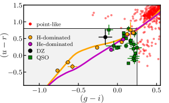
Figure 1: The $(u-r)$ versus $(g-i)$ color-color diagram in miniJPAS for point-like sources with $r<21.5$ mag (red dots). The gray area defines the bluest point-like sources with $(u-r)<0.80$ and $(g-i)<0.25$. The $33$ sources in this area are classified from SDSS spectrum as $11$ white dwarfs ($8$ with H-dominated atmosphere, orange dots; $2$ with He-dominated atmosphere, purple dots; $1$ metal polluted DZ, black dot) and $22$ QSOs (green squares). The expected colors from theoretical cooling tracks for H-dominated and He-dominated atmospheres are shown with the orange and purple lines, respectively.

Table 1: White dwarfs in the miniJPAS bluest point-like sample: photometry and Gaia information.

Tile - Number	RA	Dec	$r$	$(g-i)$	$(u-r)$	$\varpi_{\rm EDR3}$	Reference
	[deg]	[deg]	[mag]	[mag]	[mag]	[mas]
​$2241-1747$	214.1778	52.2620	$19.32\pm 0.01$	$-0.08\pm 0.01$	$0.17\pm 0.02$	$4.36\pm 0.34$	1
$2241-19527$	214.5030	52.4108	$19.61\pm 0.01$	$-0.26\pm 0.02$	$0.23\pm 0.03$	$4.95\pm 0.24$	1,2
$2243-2625$	214.3501	52.8745	$19.30\pm 0.01$	$0.05\pm 0.01$	$0.40\pm 0.04$	$5.37\pm 0.19$	1,2
$2243-4859$	214.7533	52.7319	$21.48\pm 0.04$	$-0.15\pm 0.09$	$0.54\pm 0.24$	$\cdots$	$\cdots$
$2243-5175$	214.9642	52.6212	$21.12\pm 0.03$	$-0.58\pm 0.06$	$-0.34\pm 0.08$	$-2.6\pm 1.5$	1
$2406-5601$	215.3567	53.0818	$19.00\pm 0.01$	$0.20\pm 0.01$	$0.67\pm 0.03$	$7.35\pm 0.15$	1,2
$2406-9645$	215.1359	53.2736	$19.33\pm 0.01$	$0.07\pm 0.01$	$0.47\pm 0.03$	$6.31\pm 0.19$	1,2
$2406-16326$	215.7065	53.0915	$21.12\pm 0.03$	$0.17\pm 0.06$	$0.76\pm 0.23$	$\cdots$	$\cdots$
$2470-3588$	213.4513	52.1572	$19.84\pm 0.01$	$-0.77\pm 0.02$	$-0.46\pm 0.02$	$1.49\pm 0.24$	1,2
$2470-13619$	214.0558	52.1936	$20.46\pm 0.01$	$0.12\pm 0.03$	$0.63\pm 0.07$	$1.99\pm 0.55$	1,2
$2470-15262$	214.0462	52.1328	$20.55\pm 0.02$	$-0.63\pm 0.04$	$-0.21\pm 0.04$	$0.37\pm 0.53$	1

(1) Gaia Collaboration et al. (2021a); (2) Included in the Gentile Fusillo et al. (2021) catalog based on Gaia EDR3 with white dwarf probability $P_{\rm WD}>0.75$.

Table 2: White dwarfs in the miniJPAS bluest point-like sample: Atmospheric parameters from SDSS spectroscopy.

Tile - Number	SDSS	Type	Composition	$T_{\rm eff}^{\rm spec}$	$\log{\rm g}^{\rm spec}$	Reference
	Plate-MJD-Fiber			[K]	[dex]
​$2241-1747$	7028-56449-0220	DA	He	$5240\pm 130$	$7.6\pm 0.3$	2
$2241-19527$	7028-56449-0185	DA	H	$11\,010\pm 100$	$8.70\pm 0.06$	2
$2243-2625$	7028-56449-0199	DA	H	$7\,880\pm 60$	$7.85\pm 0.11$	2
$2243-4859$	7030-56448-0227	DZ	He	$\cdots$	$\cdots$	$\cdots$
$2243-5175$	7028-56449-0102	DA	H	$19\,300\pm 700$	$8.17\pm 0.11$	1
$2406-5601$	7028-56449-0930	DA	H	$7\,380\pm 50$	$7.78\pm 0.11$	2
$2406-9645$	6717-56397-0721	DC	He	$\cdots$	$\cdots$	$\cdots$
$2406-16326$	7031-56449-0616	DA	H	$7\,400\pm 300$	$8\pm 1$	1
$2470-3588$	7030-56448-0453	DA	H	$22\,800\pm 400$	$7.89\pm 0.06$	2
$2470-13619$	7030-56448-0380	DA	H	$8\,520\pm 120$	$7.7\pm 0.2$	2
$2470-15262$	7029-56455-0253	DA	H	$17\,600\pm 500$	$7.76\pm 0.09$	1

(1) Kepler et al. (2016); (2) Kepler et al. (2019).

Table 3: White dwarfs in the miniJPAS bluest point-like sample: fitting results from miniJPAS photometry.

Tile - Number	$p_{\rm H}$	$T_{\rm eff}$	$\log{\rm g}$	$\varpi$	$\chi^{2}_{\rm WD}$
		[K]	[dex]	[mas]
​$2241-1747$	$0.00$	$8\,510\pm 120$	$7.69\pm 0.14$	$4.4\pm 0.3$	$20.0$
$2241-19527$	$1.00$	$11\,250\pm 240$	$8.66\pm 0.06$	$4.99\pm 0.24$	$33.7$
$2243-2625$	$1.00$	$7\,850\pm 100$	$7.91\pm 0.07$	$5.40\pm 0.19$	$18.4$
$2243-4859$	$0.88$	$8\,700\pm 400$	$7.0\pm 0.7$	$1.16\pm 0.23$	$81.3$
$2243-4859$	$0.01$	$8\,800\pm 400$	$8.3\pm 0.6$	$2.2\pm 1.0$	$53.2$
$2243-5175$	$1.00$	$19\,900\pm 1\,100$	$7.8\pm 0.5$	$0.9\pm 0.3$	$52.9$
$2406-5601$	$1.00$	$7\,160\pm 80$	$7.95\pm 0.04$	$7.35\pm 0.15$	$13.2$
$2406-9645$	$0.00$	$7\,510\pm 90$	$7.99\pm 0.06$	$6.30\pm 0.19$	$36.7$
$2406-16326$	$0.99$	$7\,150\pm 180$	$8.8\pm 0.7$	$5.2\pm 3.4$	$48.3$
$2470-3588$	$1.00$	$22\,400\pm 900$	$7.87\pm 0.22$	$1.45\pm 0.20$	$47.8$
$2470-13619$	$1.00$	$8\,140\pm 180$	$7.1\pm 0.4$	$1.99\pm 0.25$	$44.9$
$2470-15262$	$1.00$	$18\,000\pm 800$	$7.6\pm 0.3$	$1.02\pm 0.21$	$52.8$

Table 4: Quasars in the miniJPAS bluest point-like sample.

Tile - Number	RA	Dec	$r$	$(g-i)$	$(u-r)$	$\varpi_{\rm EDR3}$	$z_{\rm spec}$	$\chi^{2}_{\rm WD}$
	[deg]	[deg]	[mag]	[mag]	[mag]	[mas]
​$2241-3755$	213.9637	52.4613	$19.73\pm 0.01$	$0.20\pm 0.02$	$0.66\pm 0.04$	$-0.20\pm 0.28$	$2.581$	$314.0$
$2241-7683$	214.3127	52.3869	$21.24\pm 0.03$	$0.20\pm 0.07$	$-0.09\pm 0.08$	$\cdots$	$1.260$	$131.4$
$2241-9344$	214.4118	52.3925	$21.26\pm 0.03$	$0.17\pm 0.06$	$0.36\pm 0.11$	$\cdots$	$2.159$	$472.2$
$2241-14404$	214.3972	52.6476	$20.24\pm 0.01$	$0.14\pm 0.02$	$-0.24\pm 0.03$	$0.17\pm 0.44$	$1.961$	$520.8$
$2241-20770$	214.5971	52.6679	$21.28\pm 0.03$	$0.21\pm 0.05$	$0.20\pm 0.10$	$\cdots$	$1.766$	$284.1$
$2243-12132$	215.0233	53.0102	$19.81\pm 0.01$	$0.23\pm 0.02$	$0.06\pm 0.04$	$-0.18\pm 0.28$	$1.647$	$431.4$
$2243-12352$	214.9700	53.0345	$20.47\pm 0.02$	$0.11\pm 0.03$	$0.28\pm 0.07$	$1.76\pm 0.74$	$1.902$	$265.3$
$2243-12363$	214.9946	53.0194	$20.83\pm 0.02$	$0.21\pm 0.04$	$0.32\pm 0.11$	$-1.03\pm 0.72$	$1.728$	$200.7$
$2406-853$	215.2185	52.9396	$18.14\pm 0.01$	$0.01\pm 0.01$	$0.23\pm 0.01$	$0.09\pm 0.08$	$0.676$	$430.4$
$2406-1224$	215.3250	52.8961	$20.39\pm 0.01$	$0.16\pm 0.02$	$0.43\pm 0.08$	$0.43\pm 0.37$	$2.305$	$577.3$
$2406-4342$	215.0437	53.2066	$20.09\pm 0.01$	$0.14\pm 0.02$	$0.79\pm 0.09$	$-0.68\pm 0.46$	$2.590$	$263.8$
$2406-5133$	215.3823	53.0450	$21.26\pm 0.03$	$-0.05\pm 0.10$	$0.28\pm 0.15$	$\cdots$	$0.957$	$145.0$
$2406-8977$	215.3053	53.2052	$21.21\pm 0.03$	$0.22\pm 0.05$	$-0.16\pm 0.10$	$\cdots$	$1.953$	$204.5$
$2406-11608$	215.7752	53.2581	$18.44\pm 0.01$	$0.08\pm 0.01$	$0.67\pm 0.02$	$-0.15\pm 0.13$	$2.462$	$481.1$
$2406-14008$	215.6897	53.2010	$21.34\pm 0.03$	$0.25\pm 0.06$	$0.26\pm 0.15$	$\cdots$	$1.671$	$99.6$
$2406-14869$	215.4022	53.3373	$21.48\pm 0.04$	$0.22\pm 0.06$	$-0.03\pm 0.14$	$\cdots$	$2.019$	$160.9$
$2470-2363$	213.7993	51.8822	$19.60\pm 0.01$	$0.08\pm 0.01$	$0.57\pm 0.03$	$-0.01\pm 0.22$	$2.306$	$350.4$
$2470-4230$	213.4213	52.2056	$18.96\pm 0.01$	$0.17\pm 0.01$	$0.44\pm 0.02$	$-0.05\pm 0.21$	$1.213$	$127.7$
$2470-4455$	213.4495	52.2014	$21.16\pm 0.03$	$-0.11\pm 0.05$	$0.76\pm 0.15$	$\cdots$	$2.351$	$159.8$
$2470-7732$	213.8912	52.0994	$18.15\pm 0.01$	$-0.01\pm 0.01$	$0.22\pm 0.01$	$-0.03\pm 0.10$	$0.987$	$198.3$
$2470-9064$	213.4318	52.3207	$20.49\pm 0.02$	$0.22\pm 0.03$	$0.65\pm 0.11$	$-0.94\pm 0.62$	$1.327$	$258.8$
$2470-13393$	213.6948	52.4233	$19.47\pm 0.01$	$0.11\pm 0.01$	$0.51\pm 0.03$	$-0.48\pm 0.26$	$1.583$	$313.7$

2.3 The sample of bluest point-like sources

We aim to provide a forecast for the white dwarf science with the J-PAS 56 optical filters. Our working sample is composed of the bluest point-like sources (BPS) in the miniJPAS catalog, where mainly white dwarfs and extragalactic QSOs are expected. To define the BPS catalog, magnitudes from $3$ arcsec photometry corrected by aperture effects were used.

The point-like sample was defined with apparent magnitude $r<21.5$ mag to ensure a large enough ${\rm S/N}$ in the medium-band photometry. This magnitude selection translates to a median ${\rm S/N}$ per passband larger than $5$ in all the BPS. We also imposed a probability of being point-like of $p_{\rm point}>0.5$. We obtained a total of $2\,684$ sources with these criteria.

Then, a colour selection was performed in the $(u-r)$ versus $(g-i)$ color diagram (Fig. 1). We used these colors to ensure independent measurements and avoid correlated uncertainties. Several structures are apparent in this color-color plot. White dwarfs occupy the bluest corner in the plot, as illustrated with the H-dominated and He-dominated theoretical cooling tracks (see Sect. 3, for details about the assumed models). A sparsely populated sequence, corresponding to A-type and blue horizontal branch stars, is at $(g-i)\lesssim 0.3$ mag and $(u-r)\sim 1.2$ mag. The common F-type stars produce the overdensity at $(g-i)\sim 0.4$ mag and $(u-r)\sim 1.3$ mag. Finally, the QSO population is responsible for the data excess visible at $(g-i)\sim 0.3$ and $(u-r)\sim 0.3$ mag.

We defined the bluest sources in miniJPAS with $(u-r)<0.80$ mag and $(g-i)<0.25$ mag. These color selections ensure a complete sample for white dwarfs at $T_{\rm eff}\gtrsim 7\,000$ K, as expected from the theoretical cooling tracks described in Sect. 3, and minimise the contamination from main sequence stars and QSOs. The selection provided a total of $33$ sources in the surveyed area of one square degree, defining the BPS sample.

The next step was to gather all the available information about the BPS in the literature. We searched for information in the Montreal white dwarf database (Dufour et al. 2017) and Simbad (Wenger et al. 2000). We also collected SDSS spectroscopy and Gaia EDR3 (Gaia Collaboration et al. 2021a) astrometry. We found that all the BPS have a SDSS spectrum, providing a spectral classification of the sources. The BPS sample was split into $11$ white dwarfs (Tables 1, 2, and 3) and $22$ QSOs (Table 4).

We study the physical properties of the $11$ white dwarfs in Sect. 4, and state the capabilities of miniJPAS photometry to disentangle between white dwarfs and QSOs in Sect. 5.

3 Bayesian estimation of white dwarf atmospheric parameters and composition

The Bayesian methodology used to analyse the miniJPAS data was developed in López-Sanjuan et al. (2022) to study the white dwarf population in the Javalambre Photometric Local Universe Survey (J-PLUS, Cenarro et al. 2019), comprising $12$ optical filters. We adapted the method to deal with the $56$ medium bands in miniJPAS and included in the analysis the $g$ and $i$ broad bands. The $u_{\rm J}$ and $r$ broad bands were not used because they have been discarded from the final J-PAS observing strategy, that will only include $g$ and $i$. We provide in the following a summary of the fitting process, that is fully detailed in López-Sanjuan et al. (2022).

We estimated the normalized probability density function (PDF) for each white dwarf in the sample,

$${\rm PDF}\,(t,\theta\,|\,\@vec{f},\@vec{\sigma}_{\@vec{f}})\propto\mathcal{L}\,(\,\@vec{f}\,|\,t,\theta,\sigma_{\@vec{f}})\times P\,(\varpi),$$ (2)

where $t=\{{\rm H},{\rm He}\}$ are the explored H- and He-dominated atmosphere compositions, $\theta=\{T_{\rm eff},\log g,\varpi\}$ are the parameters in the fitting (effective temperature, surface gravity, and parallax), $\mathcal{L}$ is the likelihood of the data for a given set of parameters and atmospheric composition, and $P$ is the prior probability imposed to the parallax.

The likelihood was defined as

$$\mathcal{L}\,(\,\@vec{f}\,|\,t,\theta,{\boldmath\sigma}_{\@vec{f}})=\prod_{j=1}^{58}P_{\rm G}\,(f_{j}\,|\,f_{t,j}^{\rm mod},\sigma_{j}),$$ (3)

where the index $j$ runs over the $56$ medium bands and the $gi$ broad bands in miniJPAS, the function $P_{\rm G}$ defines a Gaussian distribution with median $\mu$ and dispersion $\sigma$, and the model flux was

$$f_{t,j}^{\rm mod}\,(t,\theta)=\bigg{(}\frac{\varpi}{100}\bigg{)}^{2}\,F_{t,k}\,(T_{\rm eff},\log g)\,10^{0.4\,k_{j}\,E(B-V)}\,10^{0.4\,C^{\rm aper}_{j}},$$ (4)

where $k_{j}$ is the extinction coefficient of the filter, $E(B-V)$ the colour excess of the source, $C^{\rm aper}_{j}$ is the aperture correction needed to translate the observed $3$ arcsec fluxes to total fluxes (Sect. 2.2), and $F_{t,k}$ is the theoretical absolute flux emitted by a white dwarf at 10 pc distance. The uncertainty in the photometric calibration ($\sigma_{\rm cal}=0.04$ mag) was included in the error vector.

The color excess was estimated by using the 3D reddening map from Green et al. (2018) at distance $d=\varpi^{-1}$. We note that this extinction correction was used in the photometric calibration of miniJPAS, so we also used it for consistency.

Pure-H models were assumed to describe H-dominated atmospheres ($t={\rm H}$, Tremblay et al. 2011, 2013). Mixed models with H/He = $10^{-5}$ at $T_{\rm eff}>6\,500$ K and pure-He models at $T_{\rm eff}<6\,500$ K were used to define He-dominated atmospheres ($t={\rm He}$, Cukanovaite et al. 2018, 2019). The mass-radius relation of Fontaine et al. (2001) for thin (He-atmospheres) and thick (H-atmospheres) hydrogen layers were used in the modelling. The justification of these choices and extended details about the assumed models can be found in Bergeron et al. (2019); Gentile Fusillo et al. (2020, 2021); and McCleery et al. (2020).

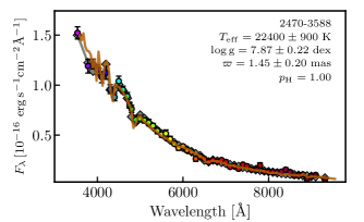
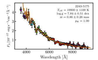
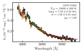
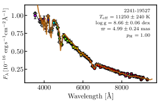
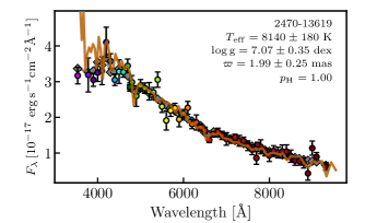
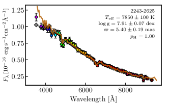
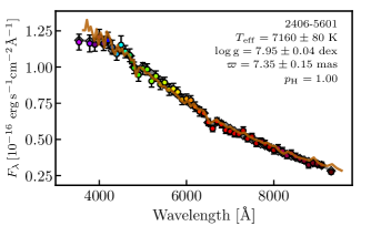
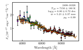
Figure 2: Photo-spectra of the miniJPAS sources classified as H-dominated DAs in descending effective temperature from top-left to bottom-right. Colored circles represent the 56 medium bands, and squares indicate the $g$ and $i$ broad bands. The presented fluxes were estimated from the $3$ arsec diameter aperture photometry corrected for aperture effects (Sect. 2.2) and no correction for interstellar reddening was applied. The gray diamonds show the theoretical flux form the best-fitting model to the data. The parameters of the fitting are labelled in the panel. The brown solid line depicts the SDSS spectra of the sources with a downgraded resolution of $R\sim 90$ for a better comparison. The flux of the SDSS spectra were scaled to match the miniJPAS $r$-band photometry. The flux scale of the SDSS spectra for the sources $2243-2625$, $2406-5601$, and $2406-16326$ has an additional factor $(\lambda/\lambda_{0})^{a}$ applied, with $\lambda_{0}=6\,254\,\AA$ and $a=1.1,0.3$, and $-0.4$, respectively.

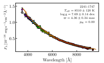
Figure 3: Photo-spectrum of the miniJPAS source 2241-1747 (He-rich DA). Symbols as in Fig.  2.

The prior probability in the parallax was

$$P\,(\varpi)=P_{\rm G}\,(\varpi\,|\,\varpi_{\rm EDR3},\sigma_{\varpi}),$$ (5)

where $\varpi_{\rm EDR3}$ and $\sigma_{\varpi}$ are the parallax and its error from ${\it Gaia}$ EDR3 (Gaia Collaboration et al. 2021a; Lindegren et al. 2021b). The published values of the parallax were corrected using the prescription in Lindegren et al. (2021a). In all cases, only positive values of the parallax ($\varpi\leavevmode\nobreak\ >\leavevmode\nobreak\ 0$) were allowed.

Finally, the probability of having a H-dominated atmosphere was

$$p_{\rm H}=\int{\rm PDF}\,({\rm H},\theta)\,{\rm d}\theta.$$ (6)

The reported values of each parameter in the Tables were estimated by marginalizing over the other parameters at the dominant atmospheric composition defined by $p_{\rm H}$ and performing a Gaussian fit to the obtained distribution. The parameter and its uncertainty are the median and the dispersion of the best-fitting Gaussian.

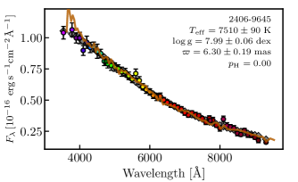
Figure 4: Photo-spectrum of the miniJPAS source 2406-9645 (DC). Symbols as in Fig. 2. The flux scale of the SDSS spectrum has an additional factor $(\lambda/\lambda_{0})^{0.3}$ applied, with $\lambda_{0}=6\,254$ Å.

4 Analysis of the white dwarf population in miniJPAS

This section is devoted to the analysis of the white dwarf population in the BPS sample. We provide the relevant individual results for the 11 white dwarfs in Sect. 4.1. The performance in the estimation of the effective temperature and the surface gravity is presented in Sect. 4.2. The capabilities of the J-PAS filter system to derive the white dwarf atmospheric composition are discussed in Sect. 4.3.

4.1 Notes on individual objects

In this section, we present the relevant results for the 9 DAs (Sect. 4.1.1), the DC (Sect. 4.1.2), and the DZ (Sect. 4.1.3) in the BPS sample. All the sources have SDSS spectrum, but in several cases a mismatch between the spectrum and the miniJPAS photometry was evident. Such discrepancies have been also reported by Hollands et al. (2017). We found that both data sets can be reconciled by simply multiplying the SDSS spectrum by a factor $(\lambda/\lambda_{0})^{a}$, with $\lambda_{0}=6\,254\,\AA$ and $a$ depending on each individual source.

4.1.1 DA spectral type

There are eight H-dominated DAs and one He-rich DA in the analyzed sample. These sources are presented in Fig. 2, ordered by decreasing effective temperature. We find that the miniJPAS photometry shows H$\alpha$, H$\beta$, H$\gamma$, and H$\delta$ in most of the cases. The intensity of the Balmer lines is also well recovered by the miniJPAS photo-spectra. We obtained $p_{\rm H}\geq 0.99$ for all the H-dominated DAs. The effective temperature and surface gravity from miniJPAS photometry are compatible with the spectroscopic values at $2\sigma$ level in all the cases (Sect. 4.2).

The source $2241-1747$ is spectroscopically classified as an He-rich DA by Kepler et al. (2016), but was classified as DC in previous studies because of its weak Balmer lines (Eisenstein et al. 2006; Kleinman et al. 2013). The analysis of the spectrum with pure-H models implies $T_{\rm eff}\sim 5\,200$ K, but the continuum suggests a hotter system. Both results can be reconciled with a He-dominated atmosphere (see Rolland et al. 2018 and Kilic et al. 2020). The miniJPAS data provide a featureless photo-spectrum (Fig. 3) with $p_{\rm H}=0$ and a shape compatible with the SDSS spectrum of the source. As expected, the photometric effective temperature is $T_{\rm eff}=8\,510\pm 120$ K, hotter by $\sim 3\,000$ K than the reported spectroscopic value when a pure-H atmosphere is assumed.

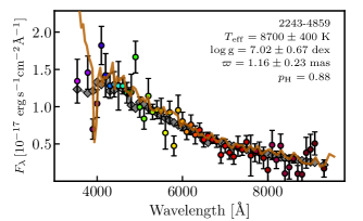
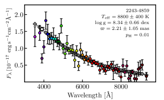
Figure 5: Photo-spectrum of the miniJPAS source 2243-4859 (DZ, $r=21.4$ mag). Symbols as in Fig. 2. Left panel: All the miniJPAS passbands were used in the fitting process. Right panel: The filters $J0390$ and $J0400$ were not included in the fitting. The expected flux in the $J0390$ passband from the modelling is marked by a white diamond.

4.1.2 DC spectral type

The source $2406-9645$ is the only object in the sample classified as DC (Fig. 4). The miniJPAS photometry is compatible with a featureless continuum, providing $p_{\rm H}=0$. We estimated $T_{\rm eff}=7\,510\pm 90$ K and $\log{\rm g}=7.99\pm 0.06$ dex.

4.1.3 DZ spectral type

The source $2243-4859$ is classified as DZ (calcium white dwarf; Fig. 5), and the Ca ii H+K absorption feature is present at $3\,950\,\AA$ in the SDSS spectrum. The miniJPAS photometry presents a clear absorption in the passbands $J0390$ and $J0400$. The parameters obtained with all the photometric data provides $p_{\rm H}=0.88$ and a low surface gravity of $\log{\rm g}=7.0\pm 0.7$ dex. We repeated the analysis without the $J0390$ and $J0400$ passbands. The solutions in this case are different, with $p_{\rm H}=0.01$ and $\log{\rm g}=8.3\pm 0.6$ dex. In both cases, the effective temperature is similar, $T_{\rm eff}\sim 8\,800$ K. We note that this object has no parallax information from Gaia EDR3. We compared the expected flux in the $J0390$ passband from the latter fitting process with the miniJPAS measurement, obtaining an equivalent width of ${\rm EW}_{J0390}=78\pm 12\ \AA$, or a 6$\sigma$ detection of the calcium absorption. The J-PAS capabilities to detect metal-polluted white dwarfs are discussed in Sect. 4.3.

4.2 Temperature and surface gravity

In this section, we compare the $T_{\rm eff}$ and $\log{\rm g}$ values obtained from miniJPAS photometry against those obtained from SDSS spectroscopy by Kepler et al. (2016, 2019), as summarised in Table 2. The DAs spectra were fitted with pure-H models (Koester 2010), including the Stark-line broadening from Tremblay & Bergeron (2009) and the 3D corrections from Tremblay et al. (2013) at $T_{\rm eff}\leq 14\,000$ K. We restricted the comparison to the eight H-dominated white dwarfs in the sample (Sect.4.1.1) for which the spectroscopic method based on pure-H theoretical models is reliable.

We found a tight one-to-one agreement in $T_{\rm eff}$, as illustrated in Fig. 6. The relative difference between both measurements is $1$%, with a dispersion of only $3$%. All the miniJPAS measurements are compatible with the spectroscopic values at $2\sigma$ level. The typical relative error in the effective temperature from miniJPAS data is $2$%, close to the $1$% estimated from spectroscopy. Additionally, the typical relative error for the general white dwarf population is $10$% from the Gaia EDR3 photometry (Gentile Fusillo et al. 2021) and $5$% from the J-PLUS photometry (López-Sanjuan et al. 2022).

As reported in Sect. 4.1, some SDSS spectra present a shape discrepancy with the miniJPAS photometry. The excellent agreement between the effective temperature from SDSS spectrum, based on the absorption features and thus insensitive to the flux normalization, and from miniJPAS photometry, mainly based on the continuum shape, points to a problematic flux calibration of the discrepant SDSS spectra.

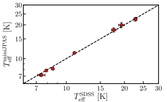
Figure 6: Effective temperature derived from miniJPAS photometry, $T_{\rm eff}^{\rm miniJPAS}$, as a function of the effective temperature derived from SDSS spectrum, $T_{\rm eff}^{\rm SDSS}$ (red dots with black error bars). The dashed line marks the one-to-one relation.

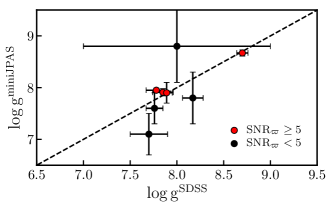
Figure 7: Surface gravity derived from miniJPAS photometry, $\log{\rm g}^{\rm miniJPAS}$, as a function of the surface gravity derived from SDSS spectrum, $\log{\rm g}^{\rm SDSS}$. Red dots mark sources with a ${\rm S/N}$ in $\varpi_{\rm EDR3}$ larger than five, and black dots are sources with a ${\rm S/N}$ lower than five. The dashed line indicates the one-to-one relation.

The surface gravity values obtained with both photo-spectra and spectroscopic data are compared in Fig. 7. We found an agreement between photometric and spectroscopic measurements. However, a precise estimation of $\log{\rm g}$ from miniJPAS photometry demands a precise parallax measurement from Gaia. The surface gravity information is mainly encoded in the widths of the lines, which are not accessible with the low-resolution miniJPAS photo-spectrum. The assumption of a mass-radius relation in the theoretical models couples the surface gravity and the parallax, so a precise parallax prior from Gaia astrometry permits to derive the surface gravity when both the effective temperature and the atmospheric composition are well constrained.

We conclude that J-PAS is able to provide effective temperatures with $\sim 2$% precision, but its spectral resolution is not large enough to retrieve a precise surface gravity without parallax information.

4.3 White dwarf atmospheric composition

The main advantage of low-resolution spectral information with respect to broad band photometry is its capability to disentangle the white dwarf main atmospheric composition. The miniJPAS medium-band photometry permits to correctly classify with $99$% confidence the $11$ white dwarfs in the sample. The hydrogen Balmer lines are visible in miniJPAS photometry of H-dominated atmospheres with temperatures ranging from $7\,000$ K to $22\,000$ K, enabling a clear separation between H- and He-dominated white dwarfs down to $T_{\rm eff}\sim 7\,000$ K. The J-PAS performance at lower and higher effective temperatures will be tested in the near future when larger samples are available.

In addition, the presence of polluting metals in the white dwarf atmosphere can be identified thanks to the filters $J0390$ and $J0400$. These passbands are sensitive to the presence of the Ca ii H+K absorption, as illustrated for the source $2243-4859$ in Fig. 5. We have estimated the equivalent width in the $J0390$ filter as described in Sect. 4.1.3 for all the white dwarfs in the sample. The significance of the measurement, estimated as ${\rm EW}_{J0390}/\sigma_{\rm EW}$, is presented in Fig. 8. Those sources classified as non-DZ cluster around zero and are compatible with the absence of calcium absorption at $2\sigma$ level. A Kolmogov-Smirnov test provides a $98$% probability that their distribution is drawn for a normal distribution, as expected if the measurements are compatible with zero within uncertainties. The only outlier is the DZ source, which presents a $6\sigma$ detection. Thus, the ${\rm EW}_{J0390}$ measurement can be used to select new metal-polluted white dwarfs. In addition to the calcium absorption, the presence of other prominent absorption features in cool white dwarfs, such as the Mg i $b$ triplet and the Na i doublet at $5\,893\ \AA$ (e.g., Hollands et al. 2017), would be also detectable in the J-PAS data.

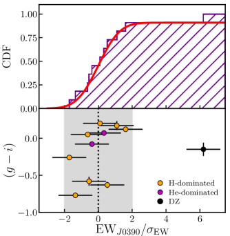
Figure 8: Distribution in the significance of the ${\rm EW}_{J0390}$ measurements as a proxy for calcium absorption in white dwarfs. Top panel: Cumulative distribution function (CDF) of the ${\rm EW}_{J0390}$ significance. The red solid line is the CDF of a normal distribution normalized to the non-DZ population. Bottom panel: The color $(g-i)$ as a function of the ${\rm EW}_{J0390}$ significance. Symbols as in Fig. 1. The dotted line marks zero and the gray area shows the $\pm 2\sigma$ interval.

Our results demonstrate that J-PAS photometry will be able to provide the main atmospheric composition for white dwarfs, including the presence of polluting metals. However, the small sample available in the miniJPAS area does not permit to study in detail the J-PAS capabilities in the estimation of either H-to-He abundances on hybrid types (e.g., DABs and DBAs) or metal abundances in polluted systems, and does not contain magnetic, carbon, or peculiar white dwarfs. The performance of the J-PAS filter system with these types will be evaluated in the future when larger samples are observed.

We conclude that J-PAS photo-spectrum will allow to accurately study the evolution of He-dominated white dwarfs and the fraction of metal-polluted white dwarfs with effective temperature at least down to $T_{\rm eff}\sim 7\,000$ K.

5 White dwarf selection based on miniJPAS photometry

We have demonstrated the capabilities of multi-band photometry in the study of known white dwarfs. This will impact the analysis of the future white dwarf samples, like those expected from Gaia data. In addition, we aim to test the performance of miniJPAS data to select new white dwarf candidates just based on optical photo-spectra. In this section, we analysed the BPS sample on this regard. For that, the model flux presented in Sect. 3 was simplified as:

$$f_{t,j}^{\rm mod}\,(t,T_{\rm eff},\log g)=C_{r}\,F_{t,k}\,(T_{\rm eff},\log g)\,10^{0.4\,k_{j}\,E(B-V)}\,10^{0.4\,C^{\rm aper}_{j}},$$ (7)

where $C_{r}$ is a constant to normalise the theoretical flux to the measured flux in the miniJPAS $r$ band. That is, we assumed a unique scale for each {$T_{\rm eff}$, $\log{\rm g}$} pair to remove the parallax as a parameter in the fitting process. The prior in parallax was also neglected to provide a consistent analysis of Galactic and extragalactic sources, and only the likelihood of being white dwarf was computed. The assumed colour excess was computed at the distance implied by the $C_{r}$ normalization.

We used this scheme to obtain the minimum $\chi^{2}$ for each object as

$$\chi^{2}_{\rm WD}=-2\times\log\mathcal{L}_{\rm max},$$ (8)

where $\mathcal{L}_{\rm max}$ is the maximum likelihood obtained in the exploration of the parameters space for both H- and He-dominated atmospheres.

We present the results in Fig. 9, and show the correspoding $\chi^{2}_{\rm WD}$ in Tables 3 and 4. We found a clear separation between white dwarfs and QSOs in the BPS sample in terms of their $\chi_{\rm WD}^{2}$, with white dwarfs having lower values.

We have $58$ photometric points and three effective parameters when the constraints from the Gaia EDR3 parallax are weak (López-Sanjuan et al. 2022). Thus, the values should tend to $\chi^{2}_{\rm WD}\approx 55$. The white dwarfs tend to $\chi^{2}_{\rm WD}\approx 53$ at the faint end, as expected. There is also a trend towards lower $\chi_{\rm WD}^{2}$ at brighter magnitudes ($r\lesssim 19.5$ mag), reflecting an overestimation of the uncertainty in the photometric calibration, that was set to $\sigma_{\rm cal}=0.04$ mag for all the passbands. The QSOs have larger values of $\chi_{\rm WD}^{2}$, reaching even $\chi_{\rm WD}^{2}=500$. This is due to the presence of emission lines in the photo-spectrum, clearly off from the expected absorption lines or the featureless spectrum for white dwarfs. The presence of the Lyman $\alpha$ line in the QSO spectrum at $z>2$ provides the most prominent differences.

We conclude that white dwarfs in the BPS sample can be selected with high confidence by imposing $\chi_{\rm WD}^{2}\leq 80$. High-purity white dwarf samples will be defined with J-PAS, complementing the astrometric information from ${\rm Gaia}$ down to $G\sim 21$ and permitting to extend the analysis beyond Gaia capabilities. As an example, of the $33$ sources in the BPS sample, $8$ (25%) do not have an entry in the Gaia EDR3 catalog and only two of them are white dwarfs (Fig. 9).

The calcium white dwarf $2243-4859$ presents $\chi_{\rm WD}^{2}=81$ if all the passbands are used in the fitting, a value that decreases to $\chi_{\rm WD}^{2}=53$ when $J0390$ and $J0400$ are removed from the analysis. This implies that these two filters are clearly discrepant with the expected white dwarf flux due to the presence of calcium absorption, and provide a way to select metal-polluted white dwarfs using multi-filter photometry (Sect. 4.3). We checked that no QSO were located below the $\chi_{\rm WD}^{2}=80$ limit when the $J0390$ and $J0400$ passbands are removed from the analysis.

Finally, we searched for white dwarf candidates in the Gaia-based catalog presented by Gentile Fusillo et al. (2021). Following the authors’ suggestion, we only kept those sources with a white dwarf probability larger than $0.75$. We found six sources with $r<20.5$ mag (Fig. 9 and Table 1). Two of the four sources with $r>20.5$ mag present low ${\rm S/N}$ in the parallax and the other two have no parallax measurement. There is one bright source not included in the catalog, $2241-1747$. This source was discarded by Gentile Fusillo et al. (2021) because of the presence of a fainter, close source that increases the number of parameters in the solved astrometric solution. This exercise suggests that we could double the number of high-confidence white dwarfs in the J-PAS area with respect to Gaia-based catalogs.

A complete analysis of the BPS sample demands the addition of QSO models. This is beyond the scope of the present paper, and we demonstrated that the comparison between miniJPAS photometry and the white dwarf theoretical models is enough to discriminate the QSOs in the bluest sources at $r\leq 21.5$ mag thanks to the $56$ medium bands in the J-PAS photometric system.

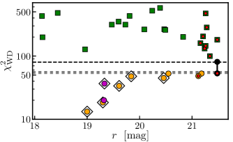
Figure 9: Minimum $\chi^{2}_{\rm WD}$ as a function of the $r$-band magnitude for the BPS. Circles mark spectroscopic white dwarfs (H-dominated: orange, He-dominated: purple, metal polluted: black), and green squares show QSOs. The values obtained with and without the filters $J0390$ and $J0410$ for the calcium white dwarf $2243-4859$ are connected by a black line. Those sources without Gaia EDR3 parallax information are marked with a red dot. Those white dwarfs included in the Gentile Fusillo et al. (2021) catalog are marked with a white diamond. The black dashed line depicts the separation between white dwarfs and QSOs, $\chi^{2}_{\rm WD}=80$. The dotted line shows the expected value for white dwarfs given the degrees of freedom in the analysis, $\chi^{2}_{\rm WD}=55$.

6 Discussion and conclusions

We have analysed the physical properties of 11 white dwarfs in the miniJPAS data set, which provides low-resolution photo-spectrum thanks to a unique filter system of $56$ medium bands with ${\rm FWHM}\approx 145\ \AA$ covering continuously the optical range from $3\,500$ to $9\,300$ Å.

We found that the effective temperature determination has a typical relative error of $2$%, whereas the estimation of a precise surface gravity demands the parallax information from Gaia. Regarding the atmospheric composition, the J-PAS filter system is able to correctly classify H- and He-dominated atmosphere white dwarfs at least in the temperature range covered by the miniJPAS white dwarf sample, $7\,000<T_{\rm eff}<22\,000$ K. We also show that the presence of polluting metals can be revealed by the Ca ii H+K absorption, as traced by the $J0390$ and $J0400$ passbands. Furthermore, the miniJPAS low-resolution information is able to disentangle between white dwarfs with $T_{\rm eff}\gtrsim 7\,000$ K and extragalactic QSOs with similar broad-band colors.

The J-PAS project, which will survey thousands of square degrees in the northern sky, will provide a unique data set of several tens thousand white dwarfs down to $r\sim 21.5$ mag to analyse the fraction of He-dominated white dwarfs with $T_{\rm eff}$, search for new metal-polluted systems, derive the white dwarf luminosity function, detect unusual objects, etc.

In addition to the data-driven forecast for J-PAS, our results provide hints about the performance of the future Gaia DR3 spectro-photometry, complementing the theoretical expectations presented in Carrasco et al. (2014). The Gaia spectro-photometry will have a comparable resolution to miniJPAS data, $R=30-90$, and therefore similar capabilities are expected at the same ${\rm S/N}$ level.

There are also relevant synergies between Gaia and J-PAS that are worth noticing. On the one hand, Gaia provides a full sky data set. On the other hand, J-PAS is deeper and provides high ${\rm S/N}$ photo-spectrum even at $G=21$ mag. We envision three different regimes: (i) Bright sources with enough ${\rm S/N}$ in Gaia spectro-photometry. Two independent measurements of the white dwarf properties will be available, providing insights about systematic errors in both surveys and tests for the Gaia capabilities at the lower ${\rm S/N}$. (ii) Faint sources with enough ${\rm S/N}$ in Gaia astrometry. The combination of J-PAS photo-spectra and Gaia parallaxes will permit to define and study in detail the white dwarf population down to $G\sim 21$ mag. And (iii) white dwarf candidates beyond Gaia data, $G>21$ mag. The J-PAS photo-spectrum can provide clean samples of white dwarfs for spectroscopic follow-up in a magnitude range dominated by QSOs and without the parallax information from Gaia. In this range, the main alternative will be the use of reduced proper motions for deep, multi-epoch surveys such as the Legacy Survey for Space and Time (LSST, Ivezic et al. 2008), capable to obtain reliable white dwarf candidates down to $G\sim 23$ mag (Fantin et al. 2020).

As an illustrative example, the $11$ white dwarfs in the miniJPAS area can be split as: six sources ($55$%) included in the Gentile Fusillo et al. (2021) catalog based on Gaia EDR3 with a white dwarf probability larger than $0.75$, three sources ($27$%) with low ${\rm S/N}$ or a low quality flag in Gaia and not included in the Gentile Fusillo et al. (2021) catalog, and two white dwarfs ($18$%) without an entry on the Gaia EDR3 catalog. Hence, there is potential to double the number of high-confidence white dwarf candidates in the future J-PAS area with respect to the Gaia-based catalogs. However, this will depend on the ${\rm S/N}$ achieved at the final Gaia data release.

Finally, the J-PAS photo-spectra will complement the spectroscopic follow-up of the Gaia-selected white dwarf population planned with SDSS-V, WEAVE, and DESI in the northern sky. J-PAS will detect and characterize new white dwarfs beyond the Gaia limits, improving the selection function of the spectroscopic surveys and providing extra candidates for spectroscopic follow up.