Logarithmic convexity and impulsive controllability for the 1-D heat equation with dynamic boundary conditions

S. E. Chorfi G. El Guermai L. Maniar  and  W. Zouhair S. E. Chorfi, G. El Guermai, L. Maniar and W. Zouhair, Cadi Ayyad University, Faculty of Sciences Semlalia, LMDP, UMMISCO (IRD-UPMC), B.P. 2390, Marrakesh, Morocco chorphi@gmail.com, ghita.el.guermai@gmail.com, maniar@uca.ma, walid.zouhair.fssm@gmail.com
Abstract.

In this paper, we prove a logarithmic convexity that reflects an observability estimate at a single point of time for 1-D heat equation with dynamic boundary conditions. Consequently, we establish the impulse approximate controllability for the impulsive heat equation with dynamic boundary conditions. Moreover, we obtain an explicit upper bound of the cost of impulse control. At the end, we give a constructive algorithm for computing the impulsive control of minimal L2superscript𝐿2L^{2}-norm. We also present some numerical tests to validate the theoretical results and show the efficiency of the designed algorithm.

Key words and phrases:
Impulsive approximate controllability, impulsive control problems, Carleman commutator, logarithmic convexity, dynamic boundary conditions, Hilbert Uniqueness Method.
2020 Mathematics Subject Classification:
35R12, 49N25, 93C27.

1. Introduction and main results

Impulsive systems are of vital importance for most scientific fields; they can be found in many applications ranging from, among others, engineering, biology, population dynamics, economics, see e.g., [36, 1, 30]. Many physical phenomena are modeled via evolution equations. Controls, impulses, and dynamic boundary conditions are often added to capture either a feedback or activity characterization.

In this paper, our interest is to investigate the impulse controlled heat equation with dynamic boundary conditions given by

tψ(x,t)xxψ(x,t)=0,(x,t)(a,b)×(0,T)\{τ},ψ(x,τ)=ψ(x,τ)+𝟙ω(x)h(x),x(a,b),tψ(a,t)xψ(a,t)=0,t(0,T)\{τ},tψ(b,t)+xψ(b,t)=0,t(0,T)\{τ},ψ(a,τ)=ψ(a,τ),ψ(b,τ)=ψ(b,τ),(ψ(x,0),ψ(a,0),ψ(b,0))=(ψ0(x),c,d),x(a,b),missing-subexpressionsubscript𝑡𝜓𝑥𝑡subscript𝑥𝑥𝜓𝑥𝑡0missing-subexpression𝑥𝑡\𝑎𝑏0𝑇𝜏missing-subexpression𝜓𝑥𝜏𝜓𝑥superscript𝜏subscript1𝜔𝑥𝑥missing-subexpression𝑥𝑎𝑏missing-subexpressionsubscript𝑡𝜓𝑎𝑡subscript𝑥𝜓𝑎𝑡0missing-subexpression𝑡\0𝑇𝜏missing-subexpressionsubscript𝑡𝜓𝑏𝑡subscript𝑥𝜓𝑏𝑡0missing-subexpression𝑡\0𝑇𝜏missing-subexpression𝜓𝑎𝜏𝜓𝑎superscript𝜏missing-subexpression𝜓𝑏𝜏𝜓𝑏superscript𝜏missing-subexpression𝜓𝑥0𝜓𝑎0𝜓𝑏0superscript𝜓0𝑥𝑐𝑑missing-subexpression𝑥𝑎𝑏\displaystyle\begin{aligned} &\partial_{t}\psi(x,t)-\partial_{xx}\psi(x,t)=0,&&\qquad(x,t)\in(a,b)\times(0,T)\backslash\{\tau\},\\ &\psi(x,\tau)=\psi\left(x,\tau^{-}\right)+\mathds{1}_{\omega}(x)h(x),&&\qquad x\in(a,b),\\ &\partial_{t}\psi(a,t)-\partial_{x}\psi(a,t)=0,&&\qquad t\in(0,T)\backslash\{\tau\},\\ &\partial_{t}\psi(b,t)+\partial_{x}\psi(b,t)=0,&&\qquad t\in(0,T)\backslash\{\tau\},\\ &\psi(a,\tau)=\psi\left(a,\tau^{-}\right),\\ &\psi(b,\tau)=\psi\left(b,\tau^{-}\right),\\ &\left(\psi(x,0),\psi(a,0),\psi(b,0)\right)=\left(\psi^{0}(x),c,d\right),&&\qquad x\in(a,b),\end{aligned} (1.1)

where (a,b)𝑎𝑏\left(a,b\right)\subset\mathbb{R} is an open interval, T>0𝑇0T>0 is the final time, τ(0,T)𝜏0𝑇\tau\in(0,T) is an impulse time, (ψ0,c,d)L2(a,b)×2superscript𝜓0𝑐𝑑superscript𝐿2𝑎𝑏superscript2\left(\psi^{0},c,d\right)\in L^{2}\left(a,b\right)\times\mathbb{R}^{2} denotes the initial data, ψ(,τ)𝜓superscript𝜏\psi(\cdot,\tau^{-}) denotes the left limit of the function ψ𝜓\psi at time τ𝜏\tau, ω(a,b)double-subset-of𝜔𝑎𝑏\omega\Subset(a,b) is a nonempty open subset, and hL2(ω)superscript𝐿2𝜔h\in L^{2}(\omega) is the impulse control.

The theory of impulsive differential equations was initiated by Milman and Mishkis in 1960 [29]. Afterward, many scientists contributed to the enrichment of this theory for more general evolution equations from various theoretical and numerical aspects. Many studies have been launched on this discipline and a large number of results has been reached. Controllability and observability are among the most important properties investigated within this theory, see for instance [37, 17]. A system is controllable if we can drive the state from any initial condition to any desired target within a finite period of time either exactly or approximately. A system is observable if we can determine the state of the system based on some measured output data, see more in [8, 38].

Unlike the distributed controllability for impulsive systems that has been extensively studied in the literature, see for instance [14, 21, 27, 12, 25, 24] and the references therein, the problem of controllability with impulse controls has attracted less attention and not as many works are available in this area, we mention [7, 18, 32, 35]. In the later type, the control is a function acting only at one instant of time τ𝜏\tau. This is considerably different from the former type in which the control is acting in the whole time interval (0,T)0𝑇(0,T).

Parabolic systems with dynamic boundary conditions, especially the one-dimensional systems, appear in many models and occupy a particular attention in recent literature. For instance, they model the distribution of heat in a bar of a given length [22], the flow of heat for a solid in contact with a fluid [23], and the infiltration of water through a partially saturated porous medium (e.g., the rainfall through the soil) [26]. In the absence of impulses, the null controllability of the 1-D heat equation with dynamic boundary conditions has been recently studied in [19], Chapter 5, by using the moment method developed by Fattorini and Russell in [15].

Let us briefly recall the derivation of a 1-D heat conduction model with dynamic boundary conditions. We consider the cooling of a uniform, isotropic, thin solid bar of cylindrical form, whose lateral surface is thermally insulated and its faces are placed at x=a𝑥𝑎x=a and x=b𝑥𝑏x=b. Suppose that the two ends of the bar are placed in contact with a liquid and governed by an initial temperature ψ0superscript𝜓0\psi^{0} at time t=0𝑡0t=0.

For simplicity and without loss of generality, we shall assume that the diffusivity is the unity constant d=1𝑑1d=1. The problem then is to find the temperature ψ(x,t)𝜓𝑥𝑡\psi(x,t) of points in the bar or of the liquid at any intermediate time within a time horizon [0,T]0𝑇[0,T]. Using the law of conservation of energy and Fourier’s law on heat conduction for the interior points of the bar, we obtain the classical heat equation

tψ(x,t)xxψ(x,t)=0,(x,t)(a,b)×(0,T).formulae-sequencesubscript𝑡𝜓𝑥𝑡subscript𝑥𝑥𝜓𝑥𝑡0𝑥𝑡𝑎𝑏0𝑇\partial_{t}\psi(x,t)-\partial_{xx}\psi(x,t)=0,\qquad(x,t)\in(a,b)\times(0,T).

The fact that the gain of heat by the liquid at the bar ends is equal to the loss of heat by the bar gives rise to the dynamic boundary conditions

tψ(a,t)subscript𝑡𝜓𝑎𝑡\displaystyle\partial_{t}\psi(a,t) =xψ(a,t),t(0,T),formulae-sequenceabsentsubscript𝑥𝜓𝑎𝑡𝑡0𝑇\displaystyle=\partial_{x}\psi(a,t),\;\;\,\qquad t\in(0,T),
tψ(b,t)subscript𝑡𝜓𝑏𝑡\displaystyle\partial_{t}\psi(b,t) =xψ(b,t),t(0,T).formulae-sequenceabsentsubscript𝑥𝜓𝑏𝑡𝑡0𝑇\displaystyle=-\partial_{x}\psi(b,t),\qquad t\in(0,T).

The main aim of the model (1.1) is to control the heat distribution in the whole bar by acting only on an arbitrary internal part ω(a,b)double-subset-of𝜔𝑎𝑏\omega\Subset(a,b) at a single impulse time τ(0,T)𝜏0𝑇\tau\in(0,T).

In the multi-dimensional case of a bounded domain ΩNΩsuperscript𝑁\Omega\subset\mathbb{R}^{N}, N2𝑁2N\geq 2, with a smooth boundary Γ=ΩΓΩ\Gamma=\partial\Omega, the dynamic boundary condition takes the form

tψΓδΔΓψΓ+νψ=0,subscript𝑡subscript𝜓Γ𝛿subscriptΔΓsubscript𝜓Γsubscript𝜈𝜓0\partial_{t}\psi_{\Gamma}-\delta\Delta_{\Gamma}\psi_{\Gamma}+\partial_{\nu}\psi=0, (1.2)

where ψΓ=ψ|Γ\psi_{\Gamma}=\psi_{|\Gamma} is the trace of ψ𝜓\psi, ΔΓsubscriptΔΓ\Delta_{\Gamma} is the Laplace-Beltrami operator and νψsubscript𝜈𝜓\partial_{\nu}\psi is the normal derivative with respect to the outward unit normal vector field ν𝜈\nu. The controllability and inverse problems for the non-impulsive heat equation with the dynamic boundary condition (1.2) have been considered in the recent papers [3, 9, 28, 20, 5]. The impulse approximate controllability has been recently investigated in [13]. In all these works, the presence of the diffusion on the boundary, i.e., δ>0𝛿0\delta>0, has helped to overcome a technical difficulty in establishing observability estimates, see [28, Remark 3.3]. Such estimates for δ=0𝛿0\delta=0 (absence of boundary diffusion) still open. Motivated by the aforementioned fact, we consider in the present work the one-dimensional case where no diffusion occur on the boundary. This makes our problem of particular interest and rather different from the previous works.

To prove the approximate controllability of system (1.1), we establish an observability estimate supported at the final time T𝑇T and localized in the space subset ω𝜔\omega. This result will be done by employing a logarithmic convexity inequality based on a Carleman commutator approach, see e.g., [2, 4, 6, 31, 11]. This approach has been recently considered in [31] and [11] for heat equation with homogeneous Dirichlet and Neumann boundary conditions. In our setting, we deal with several new boundary terms that need to be absorbed. Moreover, no numerical results were presented in the previous works. Therefore, we will present an algorithm for the numerical computation of the impulse control of minimal L2superscript𝐿2L^{2}-norm. This will be achieved by adapting (to the impulsive case) the penalized Hilbert Uniqueness Method (HUM) and a Conjugate Gradient (CG) method. More precisely, the strategy that we follow is based on a formulation of the control problem under the form of a suitable convex quadratic optimization problem, which allows us to determine the minimum energy control. The interested reader can refer to the book [16] and the paper [10].

Next, we state our first main result which is an observability estimate at one instant of time. The proof is given in Section 3.

Lemma 1.1.

Let ω(a,b)double-subset-of𝜔𝑎𝑏\omega\Subset(a,b) be an open nonempty set. Let ,\langle\cdot,\cdot\rangle denote the standard inner product of L2(a,b)×2superscript𝐿2𝑎𝑏superscript2L^{2}(a,b)\times\mathbb{R}^{2} and \|\cdot\| be its corresponding norm. Then the following logarithmic convexity estimate holds

U(,T)(μeKTu(,T)L2(ω))βU(,0)1β,norm𝑈𝑇superscript𝜇superscripte𝐾𝑇subscriptnorm𝑢𝑇superscript𝐿2𝜔𝛽superscriptnorm𝑈01𝛽\|U(\cdot,T)\|\leq\left(\mu\mathrm{e}^{\frac{K}{T}}\|u(\cdot,T)\|_{L^{2}(\omega)}\right)^{\beta}\|U(\cdot,0)\|^{1-\beta}, (1.3)

where μ,K>0𝜇𝐾0\mu,K>0, β(0,1)𝛽01\beta\in(0,1) and U=(u(,),u(a,),u(b,))𝑈𝑢𝑢𝑎𝑢𝑏U=\left(u(\cdot,\cdot),u(a,\cdot),u(b,\cdot)\right) is the solution of the following system

tu(x,t)xxu(x,t)=0,(x,t)(a,b)×(0,T),tu(a,t)xu(a,t)=0,t(0,T),tu(b,t)+xu(b,t)=0,t(0,T),(u(x,0),u(a,0),u(b,0))=(u0(x),c1,d1),x(a,b).missing-subexpressionsubscript𝑡𝑢𝑥𝑡subscript𝑥𝑥𝑢𝑥𝑡0missing-subexpression𝑥𝑡𝑎𝑏0𝑇missing-subexpressionsubscript𝑡𝑢𝑎𝑡subscript𝑥𝑢𝑎𝑡0missing-subexpression𝑡0𝑇missing-subexpressionsubscript𝑡𝑢𝑏𝑡subscript𝑥𝑢𝑏𝑡0missing-subexpression𝑡0𝑇missing-subexpression𝑢𝑥0𝑢𝑎0𝑢𝑏0superscript𝑢0𝑥subscript𝑐1subscript𝑑1missing-subexpression𝑥𝑎𝑏\displaystyle\begin{aligned} &\partial_{t}u(x,t)-\partial_{xx}u(x,t)=0,&&\qquad(x,t)\in(a,b)\times(0,T),\\ &\partial_{t}u(a,t)-\partial_{x}u(a,t)=0,&&\qquad t\in(0,T),\\ &\partial_{t}u(b,t)+\partial_{x}u(b,t)=0,&&\qquad t\in(0,T),\\ &\left(u(x,0),u(a,0),u(b,0)\right)=\left(u^{0}(x),c_{1},d_{1}\right),&&\qquad x\in(a,b).\end{aligned} (1.4)

We will prove the estimate (1.3) keeping track of the explicit dependence of all the relevant constants with respect to different parameters. This will allow us to obtain an explicit upper bound for the cost of the impulsive approximate controllability of system (1.1).

Remark 1.1.

Some remarks are in order:

  • We emphasize that (1.3) is an observability inequality estimating the whole solution U=(u(,),u(a,),u(b,))𝑈𝑢𝑢𝑎𝑢𝑏U=\left(u(\cdot,\cdot),u(a,\cdot),u(b,\cdot)\right) of system (6) at terminal time T𝑇T. This is done by only using one internal observation on the first component u𝑢u, which is localized in the subset ω𝜔\omega.

  • The estimate (1.3) is of independent interest. It allows one to prove an observability inequality for the non-impulsive system from any measurable set E(0,T]𝐸0𝑇E\subset(0,T] with a positive Lebesgue measure. This can be used to study the bang-bang property for the time optimal control problem [33].

The rest of the paper is organized as follows: in Section 2, we briefly recall some results on the wellposedness of the system. In Section 3, we present the strategy to obtain the observation estimate at one point of time for system (1.1). Section 4 is devoted to the impulse approximate controllability of the system. Finally, Section 5 includes a constructive algorithm for computing the impulse control of minimal L2superscript𝐿2L^{2}-norm illustrated by numerical simulations.

2. Wellposedness of the system

In this section, we recall some results that will be useful in the sequel. We will often use the following real Hilbert space 𝕃2:=L2(a,b)×2assignsuperscript𝕃2superscript𝐿2𝑎𝑏superscript2\mathbb{L}^{2}:=L^{2}(a,b)\times\mathbb{R}^{2}, equipped with the inner product

(u,c,d),(v,c1,d1)=u,vL2(a,b)+cc1+dd1.𝑢𝑐𝑑𝑣subscript𝑐1subscript𝑑1subscript𝑢𝑣superscript𝐿2𝑎𝑏𝑐subscript𝑐1𝑑subscript𝑑1\displaystyle\langle(u,c,d),(v,c_{1},d_{1})\rangle=\langle u,v\rangle_{L^{2}(a,b)}+cc_{1}+dd_{1}.

We also consider the spaces

k:={(u,u(a),u(b)):uHk(a,b)} for k=1,2,formulae-sequenceassignsuperscript𝑘conditional-set𝑢𝑢𝑎𝑢𝑏𝑢superscript𝐻𝑘𝑎𝑏 for 𝑘12\mathbb{H}^{k}:=\left\{(u,u(a),u(b))\colon u\in H^{k}\left(a,b\right)\right\}\text{ for }k=1,2,

equipped with the standard product norms.

System (6) can be written as the following abstract Cauchy problem

(ACP) t𝐔=𝐀𝐔,0<tT,formulae-sequencesubscript𝑡𝐔𝐀𝐔0𝑡𝑇\displaystyle\partial_{t}\mathbf{U}=\mathbf{A}\mathbf{U},\quad 0<t\leq T,
(ACP) 𝐔(0)=(u0,c1,d1),𝐔0superscript𝑢0subscript𝑐1subscript𝑑1\displaystyle\mathbf{U}(0)=\left(u^{0},c_{1},d_{1}\right),

where 𝐔:=(u,u(a,),u(b,))assign𝐔𝑢𝑢𝑎𝑢𝑏\mathbf{U}:=(u,u\left(a,\cdot\right),u\left(b,\cdot\right)) and the linear operator 𝐀:D(𝐀)𝕃2𝕃2:𝐀𝐷𝐀superscript𝕃2superscript𝕃2\mathbf{A}\colon D(\mathbf{A})\subset\mathbb{L}^{2}\longrightarrow\mathbb{L}^{2} is given by

𝐀=(xx00x|x=a00x|x=b00),D(𝐀)=2.\mathbf{A}=\begin{pmatrix}\partial_{xx}&0&0\\[8.53581pt] {\partial_{x}}_{|x=a}&0&0\\[8.53581pt] {-\partial_{x}}_{|x=b}&0&0\end{pmatrix},\qquad\qquad D(\mathbf{A})=\mathbb{H}^{2}.

We recall the following generation result that has been proven in [19], Proposition 5.2.1.

Proposition 1.

The operator 𝐀𝐀\mathbf{A} is densely defined, self-adjoint and generates an analytic C0subscript𝐶0C_{0}-semigroup of contractions (et𝐀)t0subscriptsuperscripte𝑡𝐀𝑡0\left(\mathrm{e}^{t\mathbf{A}}\right)_{t\geq 0} of angle π2𝜋2\dfrac{\pi}{2} on 𝕃2superscript𝕃2\mathbb{L}^{2}.

It follows that the solution map tet𝐀𝐔0maps-to𝑡superscripte𝑡𝐀subscript𝐔0t\mapsto\mathrm{e}^{t\mathbf{A}}\mathbf{U}_{0} is infinitely many times differentiable for t>0𝑡0t>0 and et𝐀𝐔0D(𝐀m)superscripte𝑡𝐀subscript𝐔0𝐷superscript𝐀𝑚\mathrm{e}^{t\mathbf{A}}\mathbf{U}_{0}\in D\left(\mathbf{A}^{m}\right) for every 𝐔0𝕃2subscript𝐔0superscript𝕃2\mathbf{U}_{0}\in\mathbb{L}^{2} and m𝑚m\in\mathbb{N}.

On the other hand, the system (1.1) can be presented as the following impulsive Cauchy problem

(ACP){tΨ(t)=𝐀Ψ(t),(0,T){τ},Ψ(τ)=(𝟙ωh,0,0),Ψ(0)=(ψ0,c,d),(ACP)casessubscript𝑡Ψ𝑡𝐀Ψ𝑡0𝑇𝜏otherwiseΨ𝜏subscript1𝜔00otherwiseΨ0superscript𝜓0𝑐𝑑otherwise\text{(ACP)}\;\;\begin{cases}\partial_{t}\Psi(t)=\mathbf{A}\Psi(t),\quad(0,T)\setminus\{\tau\},\\ \bigtriangleup\Psi(\tau)=(\mathds{1}_{\omega}h,0,0),\\ \Psi(0)=(\psi^{0},c,d),\end{cases}

where Ψ:=(ψ,ψ(a,),ψ(b,))assignΨ𝜓𝜓𝑎𝜓𝑏\Psi:=(\psi,\psi\left(a,\cdot\right),\psi\left(b,\cdot\right)) and Ψ(τ):=Ψ(,τ)Ψ(,τ)assignΨ𝜏Ψ𝜏Ψsuperscript𝜏\bigtriangleup\Psi(\tau):=\Psi\left(\cdot,\tau\right)-\Psi\left(\cdot,\tau^{-}\right). For all Ψ0:=(ψ0,c,d)𝕃2assignsubscriptΨ0superscript𝜓0𝑐𝑑superscript𝕃2\Psi_{0}:=(\psi^{0},c,d)\in\mathbb{L}^{2}, the system (ACP) has a unique mild solution given by

Ψ(t)=et𝐀Ψ0+𝟙{tτ}(t)e(tτ)𝐀(𝟙ωh,0,0),t(0,T).formulae-sequenceΨ𝑡superscripte𝑡𝐀subscriptΨ0subscript1𝑡𝜏𝑡superscripte𝑡𝜏𝐀subscript1𝜔00𝑡0𝑇\Psi(t)=\mathrm{e}^{t\mathbf{A}}\Psi_{0}+\mathds{1}_{\{t\geq\tau\}}(t)\,\mathrm{e}^{(t-\tau)\mathbf{A}}(\mathds{1}_{\omega}h,0,0),\qquad t\in(0,T).

3. Logarithmic convexity estimate

In this section, we prove Lemma 1.1. We shall follow the strategy presented in [31] in modified form. In our context, we need to collect and treat several new boundary terms arising from the dynamic boundary condition.

Following [11], we consider the weight function Φ:[a,b]×(0,T):Φ𝑎𝑏0𝑇\Phi:[a,b]\times(0,T)\rightarrow\mathbb{R} given by

Φ(x,t)=s|xx0|24(Tt+),\Phi(x,t)=\frac{-s\left\lvert x-x_{0}\right\lvert^{2}}{4(T-t+\hbar)},

where x0ω,>0formulae-sequencesubscript𝑥0𝜔Planck-constant-over-2-pi0x_{0}\in\omega,\;\hbar>0 and s(0,1)𝑠01s\in(0,1). Let us set

φ(x)=|xx0|24andΥ(t)=Tt+,\varphi(x)=\frac{-\left\lvert x-x_{0}\right\lvert^{2}}{4}\quad\text{and}\quad\Upsilon(t)=T-t+\hbar,

then

Φ(x,t)=sφ(x)Υ(t),(x,t)[a,b]×(0,T).formulae-sequenceΦ𝑥𝑡𝑠𝜑𝑥Υ𝑡for-all𝑥𝑡𝑎𝑏0𝑇\Phi(x,t)=\frac{s\varphi(x)}{\Upsilon(t)},\qquad\forall(x,t)\in[a,b]\times(0,T).

The function φ𝜑\varphi satisfies the following properties

  • (1)

    φ(x)+|φx(x)|2=0,x[a,b]\varphi(x)+\left\lvert\varphi_{x}(x)\right\lvert^{2}=0,\;\forall x\in[a,b],

  • (2)

    φx(x)=12(xx0),x[a,b]formulae-sequencesubscript𝜑𝑥𝑥12𝑥subscript𝑥0for-all𝑥𝑎𝑏\varphi_{x}(x)=-\dfrac{1}{2}(x-x_{0}),\;\forall x\in[a,b],

  • (3)

    φxx(x)=12,x[a,b]formulae-sequencesubscript𝜑𝑥𝑥𝑥12for-all𝑥𝑎𝑏\varphi_{xx}(x)=-\dfrac{1}{2},\;\forall x\in[a,b].

Proof of Lemma 1.1.

We will divide the proof into several steps.

Step 1. Let (u0,c1,d1)𝕃2{(0,0,0)}superscript𝑢0subscript𝑐1subscript𝑑1superscript𝕃2000(u^{0},c_{1},d_{1})\in\mathbb{L}^{2}\setminus\{(0,0,0)\}. Define

F(x,t)=U(x,t)eΦ(x,t)/2,𝐹𝑥𝑡𝑈𝑥𝑡superscripteΦ𝑥𝑡2F(x,t)=U(x,t)\,\mathrm{e}^{\Phi(x,t)/2},

where U(x,t):=(u(x,t)u(a,t)u(b,t))assign𝑈𝑥𝑡matrix𝑢𝑥𝑡𝑢𝑎𝑡𝑢𝑏𝑡U(x,t):=\begin{pmatrix}u(x,t)\\ u(a,t)\\ u(b,t)\end{pmatrix} is the solution of (6) and F(x,t):=(f(x,t)f(a,t)f(b,t))assign𝐹𝑥𝑡matrix𝑓𝑥𝑡𝑓𝑎𝑡𝑓𝑏𝑡F(x,t):=\begin{pmatrix}f(x,t)\\ f(a,t)\\ f(b,t)\end{pmatrix}. Define the operator P𝑃P as follows

PF=eΦ/2(txx00x|x=at0x|x=b0t)eΦ/2F.PF=\mathrm{e}^{\Phi/2}\begin{pmatrix}\partial_{t}-\partial_{xx}&0&0\\[8.53581pt] {-\partial_{x}}_{|x=a}&\partial_{t}&0\\[8.53581pt] {\partial_{x}}_{|x=b}&0&\partial_{t}\end{pmatrix}\mathrm{e}^{-\Phi/2}F.

Then

PF=(tfxxf12f(tΦ+12|xΦ|2)+xΦxf+12xxΦftf(a,t)xf(a,t)12f(a,t)tΦ(a,t)+12xΦ(a,t)f(a,t)tf(b,t)+xf(b,t)12f(b,t)tΦ(b,t)12xΦ(b,t)f(b,t)).𝑃𝐹matrixsubscript𝑡𝑓subscript𝑥𝑥𝑓12𝑓subscript𝑡Φ12superscriptsubscript𝑥Φ2subscript𝑥Φsubscript𝑥𝑓12subscript𝑥𝑥Φ𝑓subscript𝑡𝑓𝑎𝑡subscript𝑥𝑓𝑎𝑡12𝑓𝑎𝑡subscript𝑡Φ𝑎𝑡12subscript𝑥Φ𝑎𝑡𝑓𝑎𝑡subscript𝑡𝑓𝑏𝑡subscript𝑥𝑓𝑏𝑡12𝑓𝑏𝑡subscript𝑡Φ𝑏𝑡12subscript𝑥Φ𝑏𝑡𝑓𝑏𝑡PF=\begin{pmatrix}\partial_{t}f-\partial_{xx}f-\frac{1}{2}f\left(\partial_{t}\Phi+\frac{1}{2}|\partial_{x}\Phi|^{2}\right)+\partial_{x}\Phi\partial_{x}f+\frac{1}{2}\partial_{xx}\Phi f\\[8.53581pt] \partial_{t}f(a,t)-\partial_{x}f(a,t)-\frac{1}{2}f(a,t)\partial_{t}\Phi(a,t)+\frac{1}{2}\partial_{x}\Phi(a,t)f(a,t)\\[8.53581pt] \partial_{t}f(b,t)+\partial_{x}f(b,t)-\frac{1}{2}f(b,t)\partial_{t}\Phi(b,t)-\frac{1}{2}\partial_{x}\Phi(b,t)f(b,t)\end{pmatrix}.

Let us define P1subscript𝑃1P_{1} as follows

P1F=(xxf+12f(tΦ+12|xΦ|2)xΦxf12xxΦfxf(a,t)+12f(a,t)tΦ(a,t)12xΦ(a,t)f(a,t)xf(b,t)+12f(b,t)tΦ(b,t)+12xΦ(b,t)f(b,t)).subscript𝑃1𝐹matrixsubscript𝑥𝑥𝑓12𝑓subscript𝑡Φ12superscriptsubscript𝑥Φ2subscript𝑥Φsubscript𝑥𝑓12subscript𝑥𝑥Φ𝑓subscript𝑥𝑓𝑎𝑡12𝑓𝑎𝑡subscript𝑡Φ𝑎𝑡12subscript𝑥Φ𝑎𝑡𝑓𝑎𝑡subscript𝑥𝑓𝑏𝑡12𝑓𝑏𝑡subscript𝑡Φ𝑏𝑡12subscript𝑥Φ𝑏𝑡𝑓𝑏𝑡P_{1}F=\begin{pmatrix}\partial_{xx}f+\frac{1}{2}f\left(\partial_{t}\Phi+\frac{1}{2}|\partial_{x}\Phi|^{2}\right)-\partial_{x}\Phi\partial_{x}f-\frac{1}{2}\partial_{xx}\Phi f\\[8.53581pt] \partial_{x}f(a,t)+\frac{1}{2}f(a,t)\partial_{t}\Phi(a,t)-\frac{1}{2}\partial_{x}\Phi(a,t)f(a,t)\\[8.53581pt] -\partial_{x}f(b,t)+\frac{1}{2}f(b,t)\partial_{t}\Phi(b,t)+\frac{1}{2}\partial_{x}\Phi(b,t)f(b,t)\end{pmatrix}.

Since U𝑈U solves (6), then PF=0𝑃𝐹0PF=0. Thus

(tf(x,t)tf(a,t)tf(b,t))=P1F(x,t),(x,t)(a,b)×(0,T).formulae-sequencematrixsubscript𝑡𝑓𝑥𝑡subscript𝑡𝑓𝑎𝑡subscript𝑡𝑓𝑏𝑡subscript𝑃1𝐹𝑥𝑡for-all𝑥𝑡𝑎𝑏0𝑇\begin{pmatrix}\partial_{t}f(x,t)\\ \partial_{t}f(a,t)\\ \partial_{t}f(b,t)\end{pmatrix}=P_{1}F(x,t),\qquad\forall(x,t)\in(a,b)\times(0,T).

Let us compute the adjoint operator of P1.subscript𝑃1P_{1}. For any G:=(gg(a)g(b))1assign𝐺matrix𝑔𝑔𝑎𝑔𝑏superscript1G:=\begin{pmatrix}g\\ g(a)\\ g(b)\end{pmatrix}\in\mathbb{H}^{1},

P1F,Gsubscript𝑃1𝐹𝐺\displaystyle\left\langle P_{1}F,G\right\rangle =abxxfgdx+ab12fg(tΦ+12|xΦ|2)dxabgxΦxfdxabsentsuperscriptsubscript𝑎𝑏subscript𝑥𝑥𝑓𝑔d𝑥superscriptsubscript𝑎𝑏12𝑓𝑔subscript𝑡Φ12superscriptsubscript𝑥Φ2differential-d𝑥superscriptsubscript𝑎𝑏𝑔subscript𝑥Φsubscript𝑥𝑓d𝑥\displaystyle=\displaystyle\int_{a}^{b}\partial_{xx}fg\mathrm{d}x+\int_{a}^{b}\frac{1}{2}fg\left(\partial_{t}\Phi+\frac{1}{2}|\partial_{x}\Phi|^{2}\right)\mathrm{d}x-\int_{a}^{b}g\partial_{x}\Phi\partial_{x}f\mathrm{d}x
12abxxΦfgdx+xf(a,t)g(a)+12f(a,t)g(a)tΦ(a,t)12superscriptsubscript𝑎𝑏subscript𝑥𝑥Φ𝑓𝑔d𝑥subscript𝑥𝑓𝑎𝑡𝑔𝑎12𝑓𝑎𝑡𝑔𝑎subscript𝑡Φ𝑎𝑡\displaystyle-\displaystyle\frac{1}{2}\int_{a}^{b}\partial_{xx}\Phi fg\mathrm{d}x+\partial_{x}f(a,t)g(a)+\frac{1}{2}f(a,t)g(a)\partial_{t}\Phi(a,t)
12xΦ(a,t)f(a,t)g(a)xf(b,t)g(b)+12f(b,t)g(b)tΦ(b,t)12subscript𝑥Φ𝑎𝑡𝑓𝑎𝑡𝑔𝑎subscript𝑥𝑓𝑏𝑡𝑔𝑏12𝑓𝑏𝑡𝑔𝑏subscript𝑡Φ𝑏𝑡\displaystyle-\frac{1}{2}\partial_{x}\Phi(a,t)f(a,t)g(a)-\partial_{x}f(b,t)g(b)+\frac{1}{2}f(b,t)g(b)\partial_{t}\Phi(b,t)
+12xΦ(b,t)f(b,t)g(b)12subscript𝑥Φ𝑏𝑡𝑓𝑏𝑡𝑔𝑏\displaystyle+\frac{1}{2}\partial_{x}\Phi(b,t)f(b,t)g(b)
=xf(b,t)g(b)xf(a,t)g(a)abxfxgdxabsentsubscript𝑥𝑓𝑏𝑡𝑔𝑏subscript𝑥𝑓𝑎𝑡𝑔𝑎superscriptsubscript𝑎𝑏subscript𝑥𝑓subscript𝑥𝑔d𝑥\displaystyle=\partial_{x}f(b,t)g(b)-\partial_{x}f(a,t)g(a)-\int_{a}^{b}\partial_{x}f\partial_{x}g\mathrm{d}x
+12abfg(tΦ+12|xΦ|2)dxxΦ(b,t)f(b,t)g(b)12superscriptsubscript𝑎𝑏𝑓𝑔subscript𝑡Φ12superscriptsubscript𝑥Φ2differential-d𝑥subscript𝑥Φ𝑏𝑡𝑓𝑏𝑡𝑔𝑏\displaystyle+\frac{1}{2}\int_{a}^{b}fg\left(\partial_{t}\Phi+\frac{1}{2}|\partial_{x}\Phi|^{2}\right)\mathrm{d}x-\partial_{x}\Phi(b,t)f(b,t)g(b)
+xΦ(a,t)f(a,t)g(a)+abxxΦfgdx+abfxΦxgdxsubscript𝑥Φ𝑎𝑡𝑓𝑎𝑡𝑔𝑎superscriptsubscript𝑎𝑏subscript𝑥𝑥Φ𝑓𝑔d𝑥superscriptsubscript𝑎𝑏𝑓subscript𝑥Φsubscript𝑥𝑔d𝑥\displaystyle+\partial_{x}\Phi(a,t)f(a,t)g(a)+\int_{a}^{b}\partial_{xx}\Phi fg\mathrm{d}x+\int_{a}^{b}f\partial_{x}\Phi\partial_{x}g\mathrm{d}x
12abxxΦfgdx+xf(a,t)g(a)+12f(a,t)g(a)tΦ(a,t)12superscriptsubscript𝑎𝑏subscript𝑥𝑥Φ𝑓𝑔d𝑥subscript𝑥𝑓𝑎𝑡𝑔𝑎12𝑓𝑎𝑡𝑔𝑎subscript𝑡Φ𝑎𝑡\displaystyle-\displaystyle\frac{1}{2}\int_{a}^{b}\partial_{xx}\Phi fg\mathrm{d}x+\partial_{x}f(a,t)g(a)+\frac{1}{2}f(a,t)g(a)\partial_{t}\Phi(a,t)
12xΦ(a,t)f(a,t)g(a)xf(b,t)g(b)+12f(b,t)g(b)tΦ(b,t)12subscript𝑥Φ𝑎𝑡𝑓𝑎𝑡𝑔𝑎subscript𝑥𝑓𝑏𝑡𝑔𝑏12𝑓𝑏𝑡𝑔𝑏subscript𝑡Φ𝑏𝑡\displaystyle-\frac{1}{2}\partial_{x}\Phi(a,t)f(a,t)g(a)-\partial_{x}f(b,t)g(b)+\frac{1}{2}f(b,t)g(b)\partial_{t}\Phi(b,t)
+12xΦ(b,t)f(b,t)g(b)12subscript𝑥Φ𝑏𝑡𝑓𝑏𝑡𝑔𝑏\displaystyle+\frac{1}{2}\partial_{x}\Phi(b,t)f(b,t)g(b)
=f(b,t)xg(b)+f(a,t)xg(a)+abfxxgdxabsent𝑓𝑏𝑡subscript𝑥𝑔𝑏𝑓𝑎𝑡subscript𝑥𝑔𝑎superscriptsubscript𝑎𝑏𝑓subscript𝑥𝑥𝑔d𝑥\displaystyle=-f(b,t)\partial_{x}g(b)+f(a,t)\partial_{x}g(a)+\int_{a}^{b}f\partial_{xx}g\mathrm{d}x
+12abfg(tΦ+12|xΦ|2)dx12xΦ(b,t)f(b,t)g(b)\displaystyle+\frac{1}{2}\int_{a}^{b}fg\left(\partial_{t}\Phi+\frac{1}{2}\lvert\partial_{x}\Phi\lvert^{2}\right)\mathrm{d}x-\frac{1}{2}\partial_{x}\Phi(b,t)f(b,t)g(b)
+12xΦ(a,t)f(a,t)g(a)+12abxxΦfgdx+abfxΦxgdx12subscript𝑥Φ𝑎𝑡𝑓𝑎𝑡𝑔𝑎12superscriptsubscript𝑎𝑏subscript𝑥𝑥Φ𝑓𝑔d𝑥superscriptsubscript𝑎𝑏𝑓subscript𝑥Φsubscript𝑥𝑔d𝑥\displaystyle+\frac{1}{2}\partial_{x}\Phi(a,t)f(a,t)g(a)+\frac{1}{2}\int_{a}^{b}\partial_{xx}\Phi fg\mathrm{d}x+\int_{a}^{b}f\partial_{x}\Phi\partial_{x}g\mathrm{d}x
+12f(a,t)g(a)tΦ(a,t)+12f(b,t)g(b)tΦ(b,t)12𝑓𝑎𝑡𝑔𝑎subscript𝑡Φ𝑎𝑡12𝑓𝑏𝑡𝑔𝑏subscript𝑡Φ𝑏𝑡\displaystyle+\frac{1}{2}f(a,t)g(a)\partial_{t}\Phi(a,t)+\frac{1}{2}f(b,t)g(b)\partial_{t}\Phi(b,t)
=F,P1G.absent𝐹superscriptsubscript𝑃1𝐺\displaystyle=\left\langle F,P_{1}^{*}G\right\rangle.

Next, we introduce the following operator

𝒜=P1P12=(xΦx12xxΦ00012xΦ(a,t)00012xΦ(b,t)),𝒜subscript𝑃1superscriptsubscript𝑃12matrixsubscript𝑥Φsubscript𝑥12subscript𝑥𝑥Φ00012subscript𝑥Φ𝑎𝑡00012subscript𝑥Φ𝑏𝑡\mathcal{A}=\frac{P_{1}-P_{1}^{*}}{2}=\begin{pmatrix}-\partial_{x}\Phi\partial_{x}-\frac{1}{2}\partial_{xx}\Phi&0&0\\[8.53581pt] 0&-\frac{1}{2}\partial_{x}\Phi(a,t)&0\\[8.53581pt] 0&0&\frac{1}{2}\partial_{x}\Phi(b,t)\end{pmatrix},

which is antisymmetric on 1superscript1\mathbb{H}^{1}. Similarly, we define the following operator

𝒮=P1+P12=(xx+η00x|x=a12tΦ(a,t)0x|x=b012tΦ(b,t)),\mathcal{S}=\frac{P_{1}+P_{1}^{*}}{2}=\begin{pmatrix}\partial_{xx}+\eta&0&0\\[8.53581pt] {\partial_{x}}_{|x=a}&\frac{1}{2}\partial_{t}\Phi(a,t)&0\\[8.53581pt] -{\partial_{x}}_{|x=b}&0&\frac{1}{2}\partial_{t}\Phi(b,t)\end{pmatrix},\\

that is symmetric on 1superscript1\mathbb{H}^{1}, where

η=12(tΦ+12|xΦ|2).\eta=\frac{1}{2}\left(\partial_{t}\Phi+\frac{1}{2}\left\lvert\partial_{x}\Phi\right\lvert^{2}\right).\\

Thus,

tF=𝒮F+𝒜F.subscript𝑡𝐹𝒮𝐹𝒜𝐹\partial_{t}F=\mathcal{S}F+\mathcal{A}F.

Step 2. Multiplying the above equation by F𝐹F, we obtain

12tF2𝒮F,F=0.12subscript𝑡superscriptnorm𝐹2𝒮𝐹𝐹0\frac{1}{2}\partial_{t}\|F\|^{2}-\left\langle\mathcal{S}F,F\right\rangle=0.

We define the frequency function by

𝒩=𝒮F,FF2.𝒩𝒮𝐹𝐹superscriptnorm𝐹2\mathcal{N}=\frac{\langle-\mathcal{S}F,F\rangle}{\|F\|^{2}}.

Then

12tF2+𝒩F2=0.12subscript𝑡superscriptnorm𝐹2𝒩superscriptnorm𝐹20\frac{1}{2}\partial_{t}\|F\|^{2}+\mathcal{N}\|F\|^{2}=0.

The derivative of 𝒩𝒩\mathcal{N} satisfies

ddt𝒩1F2((𝒮+[𝒮,𝒜])F,Fxf(b,t)[𝒜1f(b,t)𝒜3f(b,t)]xf(a,t)[𝒜2f(a,t)𝒜1f(a,t)]xΦ(a,t)f(a,t)[𝒮1f(a,t)𝒮2f(a,t)]xΦ(b,t)f(b,t)[𝒮3f(b,t)𝒮1f(b,t)]),\begin{array}[c]{ll}\dfrac{\mathrm{d}}{\mathrm{d}t}\mathcal{N}&\leq\dfrac{1}{\|F\|^{2}}\bigg{(}\left\langle-\left(\mathcal{S}^{\prime}+[\mathcal{S},\mathcal{A}]\right)F,F\right\rangle-\partial_{x}f(b,t)\left[\mathcal{A}_{1}f(b,t)-\mathcal{A}_{3}f(b,t)\right]\\ &-\partial_{x}f(a,t)\left[\mathcal{A}_{2}f(a,t)-\mathcal{A}_{1}f(a,t)\right]-\partial_{x}\Phi(a,t)f(a,t)\left[\mathcal{S}_{1}f(a,t)-\mathcal{S}_{2}f(a,t)\right]\\ &-\partial_{x}\Phi(b,t)f(b,t)\left[\mathcal{S}_{3}f(b,t)-\mathcal{S}_{1}f(b,t)\right]\bigg{)},\end{array}

where 𝒮F=(𝒮1f𝒮2f(a,.)𝒮3f(b,.))\mathcal{S}F=\left(\begin{array}[]{l}\mathcal{S}_{1}f\\ \mathcal{S}_{2}f\left(a,.\right)\\ \mathcal{S}_{3}f\left(b,.\right)\end{array}\right), 𝒜F=(𝒜1f𝒜2f(a,.)𝒜3f(b,.))\mathcal{A}F=\left(\begin{array}[]{l}\mathcal{A}_{1}f\\ \mathcal{A}_{2}f\left(a,.\right)\\ \mathcal{A}_{3}f\left(b,.\right)\end{array}\right)and [𝒮,𝒜]F=𝒮𝒜F𝒜𝒮F𝒮𝒜𝐹𝒮𝒜𝐹𝒜𝒮𝐹[\mathcal{S},\mathcal{A}]F=\mathcal{S}\mathcal{A}F-\mathcal{A}\mathcal{S}F.

Indeed,

ddt𝒩dd𝑡𝒩\displaystyle\frac{\mathrm{d}}{\mathrm{d}t}\mathcal{N} =t(𝒮F,FF2)absentsubscript𝑡𝒮𝐹𝐹superscriptnorm𝐹2\displaystyle=\partial_{t}\left(\frac{\langle-\mathcal{S}F,F\rangle}{\|F\|^{2}}\right)
=1F4(t(𝒮F,F)F2+𝒮F,FtF2)absent1superscriptnorm𝐹4subscript𝑡𝒮𝐹𝐹superscriptnorm𝐹2𝒮𝐹𝐹subscript𝑡superscriptnorm𝐹2\displaystyle=\frac{1}{\|F\|^{4}}\left(\partial_{t}\left(\langle-\mathcal{S}F,F\rangle\right)\|F\|^{2}+\langle\mathcal{S}F,F\rangle\partial_{t}\|F\|^{2}\right)
=1F2[𝒮F,F2𝒮F,F]+2F4𝒮F,F2absent1superscriptnorm𝐹2delimited-[]superscript𝒮𝐹𝐹2𝒮𝐹superscript𝐹2superscriptnorm𝐹4superscript𝒮𝐹𝐹2\displaystyle=\frac{1}{\|F\|^{2}}\left[\left\langle-\mathcal{S}^{\prime}F,F\right\rangle-2\left\langle\mathcal{S}F,F^{\prime}\right\rangle\right]+\frac{2}{\|F\|^{4}}\langle\mathcal{S}F,F\rangle^{2}
=1F2[𝒮F,F2𝒮F,𝒜F]+2F4[𝒮F2F2+𝒮F,F2]absent1superscriptnorm𝐹2delimited-[]superscript𝒮𝐹𝐹2𝒮𝐹𝒜𝐹2superscriptnorm𝐹4delimited-[]superscriptnorm𝒮𝐹2superscriptnorm𝐹2superscript𝒮𝐹𝐹2\displaystyle=\frac{1}{\|F\|^{2}}\left[\left\langle-\mathcal{S}^{\prime}F,F\right\rangle-2\langle\mathcal{S}F,\mathcal{A}F\rangle\right]+\frac{2}{\|F\|^{4}}\left[-\|\mathcal{S}F\|^{2}\|F\|^{2}+\langle\mathcal{S}F,F\rangle^{2}\right]
1F2[𝒮F,F2𝒮F,𝒜F].absent1superscriptnorm𝐹2delimited-[]superscript𝒮𝐹𝐹2𝒮𝐹𝒜𝐹\displaystyle\leq\frac{1}{\|F\|^{2}}\left[\left\langle-\mathcal{S}^{\prime}F,F\right\rangle-2\langle\mathcal{S}F,\mathcal{A}F\rangle\right]. (3.1)

Next, we calculate 2𝒮F,𝒜F2𝒮𝐹𝒜𝐹2\langle\mathcal{S}F,\mathcal{A}F\rangle,

𝒮F,𝒜F𝒮𝐹𝒜𝐹\displaystyle\langle\mathcal{S}F,\mathcal{A}F\rangle =ab(xxf+ηf)𝒜1fdx+xf(a,t)𝒜2f(a,t)+12tΦ(a,t)f(a,t)𝒜2f(a,t)absentsuperscriptsubscript𝑎𝑏subscript𝑥𝑥𝑓𝜂𝑓subscript𝒜1𝑓differential-d𝑥subscript𝑥𝑓𝑎𝑡subscript𝒜2𝑓𝑎𝑡12subscript𝑡Φ𝑎𝑡𝑓𝑎𝑡subscript𝒜2𝑓𝑎𝑡\displaystyle=\int_{a}^{b}\left(\partial_{xx}f+\eta f\right)\mathcal{A}_{1}f\mathrm{d}x+\partial_{x}f(a,t)\mathcal{A}_{2}f(a,t)+\frac{1}{2}\partial_{t}\Phi(a,t)f(a,t)\mathcal{A}_{2}f(a,t)
xf(b,t)𝒜3f(b,t)+12tΦ(b,t)f(b,t)𝒜3f(b,t)subscript𝑥𝑓𝑏𝑡subscript𝒜3𝑓𝑏𝑡12subscript𝑡Φ𝑏𝑡𝑓𝑏𝑡subscript𝒜3𝑓𝑏𝑡\displaystyle-\partial_{x}f(b,t)\mathcal{A}_{3}f(b,t)+\frac{1}{2}\partial_{t}\Phi(b,t)f(b,t)\mathcal{A}_{3}f(b,t)
=xf(b,t)𝒜1f(b,t)xf(a,t)𝒜1f(a,t)abxfx𝒜1fdxabsentsubscript𝑥𝑓𝑏𝑡subscript𝒜1𝑓𝑏𝑡subscript𝑥𝑓𝑎𝑡subscript𝒜1𝑓𝑎𝑡superscriptsubscript𝑎𝑏subscript𝑥𝑓subscript𝑥subscript𝒜1𝑓d𝑥\displaystyle=\displaystyle\partial_{x}f(b,t)\mathcal{A}_{1}f(b,t)-\partial_{x}f(a,t)\mathcal{A}_{1}f(a,t)-\int_{a}^{b}\partial_{x}f\partial_{x}\mathcal{A}_{1}f\mathrm{d}x
+abηf𝒜1fdx+xf(a,t)𝒜2f(a,t)+12tΦ(a,t)f(a,t)𝒜2f(a,t)superscriptsubscript𝑎𝑏𝜂𝑓subscript𝒜1𝑓differential-d𝑥subscript𝑥𝑓𝑎𝑡subscript𝒜2𝑓𝑎𝑡12subscript𝑡Φ𝑎𝑡𝑓𝑎𝑡subscript𝒜2𝑓𝑎𝑡\displaystyle+\int_{a}^{b}\eta f\mathcal{A}_{1}f\mathrm{d}x+\partial_{x}f(a,t)\mathcal{A}_{2}f(a,t)+\frac{1}{2}\partial_{t}\Phi(a,t)f(a,t)\mathcal{A}_{2}f(a,t)
xf(b,t)𝒜3f(b,t)+12tΦ(b,t)f(b,t)𝒜3f(b,t)subscript𝑥𝑓𝑏𝑡subscript𝒜3𝑓𝑏𝑡12subscript𝑡Φ𝑏𝑡𝑓𝑏𝑡subscript𝒜3𝑓𝑏𝑡\displaystyle-\partial_{x}f(b,t)\mathcal{A}_{3}f(b,t)+\frac{1}{2}\partial_{t}\Phi(b,t)f(b,t)\mathcal{A}_{3}f(b,t)
=xf(b,t)𝒜1f(b,t)xf(a,t)𝒜1f(a,t)f(b,t)x𝒜1f(b,t)absentsubscript𝑥𝑓𝑏𝑡subscript𝒜1𝑓𝑏𝑡subscript𝑥𝑓𝑎𝑡subscript𝒜1𝑓𝑎𝑡𝑓𝑏𝑡subscript𝑥subscript𝒜1𝑓𝑏𝑡\displaystyle=\partial_{x}f(b,t)\mathcal{A}_{1}f(b,t)-\partial_{x}f(a,t)\mathcal{A}_{1}f(a,t)-f(b,t)\partial_{x}\mathcal{A}_{1}f(b,t)
+f(a,t)x𝒜1f(a,t)+abfxx𝒜1fdx+abηf𝒜1fdx𝑓𝑎𝑡subscript𝑥subscript𝒜1𝑓𝑎𝑡superscriptsubscript𝑎𝑏𝑓subscript𝑥𝑥subscript𝒜1𝑓d𝑥superscriptsubscript𝑎𝑏𝜂𝑓subscript𝒜1𝑓differential-d𝑥\displaystyle+f(a,t)\partial_{x}\mathcal{A}_{1}f(a,t)+\int_{a}^{b}f\partial_{xx}\mathcal{A}_{1}f\mathrm{d}x+\int_{a}^{b}\eta f\mathcal{A}_{1}f\mathrm{d}x
+xf(a,t)𝒜2f(a,t)+12tΦ(a,t)f(a,t)𝒜2f(a,t)xf(b,t)𝒜3f(b,t)subscript𝑥𝑓𝑎𝑡subscript𝒜2𝑓𝑎𝑡12subscript𝑡Φ𝑎𝑡𝑓𝑎𝑡subscript𝒜2𝑓𝑎𝑡subscript𝑥𝑓𝑏𝑡subscript𝒜3𝑓𝑏𝑡\displaystyle+\partial_{x}f(a,t)\mathcal{A}_{2}f(a,t)+\frac{1}{2}\partial_{t}\Phi(a,t)f(a,t)\mathcal{A}_{2}f(a,t)-\partial_{x}f(b,t)\mathcal{A}_{3}f(b,t)
+12tΦ(b,t)f(b,t)𝒜3f(b,t)12subscript𝑡Φ𝑏𝑡𝑓𝑏𝑡subscript𝒜3𝑓𝑏𝑡\displaystyle+\frac{1}{2}\partial_{t}\Phi(b,t)f(b,t)\mathcal{A}_{3}f(b,t)
=𝒮𝒜F,F+xf(b,t)𝒜1f(b,t)xf(a,t)𝒜1f(a,t)absent𝒮𝒜𝐹𝐹subscript𝑥𝑓𝑏𝑡subscript𝒜1𝑓𝑏𝑡subscript𝑥𝑓𝑎𝑡subscript𝒜1𝑓𝑎𝑡\displaystyle=\langle\mathcal{S}\mathcal{A}F,F\rangle+\partial_{x}f(b,t)\mathcal{A}_{1}f(b,t)-\partial_{x}f(a,t)\mathcal{A}_{1}f(a,t)
+xf(a,t)𝒜2f(a,t)xf(b,t)𝒜3f(b,t).subscript𝑥𝑓𝑎𝑡subscript𝒜2𝑓𝑎𝑡subscript𝑥𝑓𝑏𝑡subscript𝒜3𝑓𝑏𝑡\displaystyle+\partial_{x}f(a,t)\mathcal{A}_{2}f(a,t)-\partial_{x}f(b,t)\mathcal{A}_{3}f(b,t).

Therefore, we obtain

𝒮F,𝒜F𝒮𝐹𝒜𝐹\displaystyle\langle\mathcal{S}F,\mathcal{A}F\rangle =𝒮𝒜F,F+xf(b,t)[𝒜1f(b,t)𝒜3f(b,t)]absent𝒮𝒜𝐹𝐹subscript𝑥𝑓𝑏𝑡delimited-[]subscript𝒜1𝑓𝑏𝑡subscript𝒜3𝑓𝑏𝑡\displaystyle=\langle\mathcal{S}\mathcal{A}F,F\rangle+\partial_{x}f(b,t)\left[\mathcal{A}_{1}f(b,t)-\mathcal{A}_{3}f(b,t)\right]
+xf(a,t)[𝒜2f(a,t)𝒜1f(a,t)].subscript𝑥𝑓𝑎𝑡delimited-[]subscript𝒜2𝑓𝑎𝑡subscript𝒜1𝑓𝑎𝑡\displaystyle+\partial_{x}f(a,t)\left[\mathcal{A}_{2}f(a,t)-\mathcal{A}_{1}f(a,t)\right]. (3.2)

Similarly, we show that

𝒮F,𝒜F𝒮𝐹𝒜𝐹\displaystyle\langle\mathcal{S}F,\mathcal{A}F\rangle =𝒜𝒮F,F+xΦ(a,t)f(a,t)[𝒮1f(a,t)𝒮2f(a,t)]absent𝒜𝒮𝐹𝐹subscript𝑥Φ𝑎𝑡𝑓𝑎𝑡delimited-[]subscript𝒮1𝑓𝑎𝑡subscript𝒮2𝑓𝑎𝑡\displaystyle=-\langle\mathcal{A}\mathcal{S}F,F\rangle+\partial_{x}\Phi(a,t)f(a,t)\left[\mathcal{S}_{1}f(a,t)-\mathcal{S}_{2}f(a,t)\right]
+xΦ(b,t)f(b,t)[𝒮3f(b,t)𝒮1f(b,t)].subscript𝑥Φ𝑏𝑡𝑓𝑏𝑡delimited-[]subscript𝒮3𝑓𝑏𝑡subscript𝒮1𝑓𝑏𝑡\displaystyle+\partial_{x}\Phi(b,t)f(b,t)\left[\mathcal{S}_{3}f(b,t)-\mathcal{S}_{1}f(b,t)\right]. (3.3)

Combining (3) and (3) yields

2𝒮F,𝒜F=2𝒮𝐹𝒜𝐹absent\displaystyle 2\langle\mathcal{S}F,\mathcal{A}F\rangle= 𝒮𝒜F,F𝒜𝒮F,F+xf(b,t)[𝒜1f(b,t)𝒜3f(b,t)]𝒮𝒜𝐹𝐹𝒜𝒮𝐹𝐹subscript𝑥𝑓𝑏𝑡delimited-[]subscript𝒜1𝑓𝑏𝑡subscript𝒜3𝑓𝑏𝑡\displaystyle\langle\mathcal{S}\mathcal{A}F,F\rangle-\langle\mathcal{A}\mathcal{S}F,F\rangle+\partial_{x}f(b,t)\left[\mathcal{A}_{1}f(b,t)-\mathcal{A}_{3}f(b,t)\right]
+xf(a,t)[𝒜2f(a,t)𝒜1f(a,t)]+xΦ(a,t)f(a,t)[𝒮1f(a,t)𝒮2f(a,t)]subscript𝑥𝑓𝑎𝑡delimited-[]subscript𝒜2𝑓𝑎𝑡subscript𝒜1𝑓𝑎𝑡subscript𝑥Φ𝑎𝑡𝑓𝑎𝑡delimited-[]subscript𝒮1𝑓𝑎𝑡subscript𝒮2𝑓𝑎𝑡\displaystyle+\partial_{x}f(a,t)\left[\mathcal{A}_{2}f(a,t)-\mathcal{A}_{1}f(a,t)\right]+\partial_{x}\Phi(a,t)f(a,t)\left[\mathcal{S}_{1}f(a,t)-\mathcal{S}_{2}f(a,t)\right] (3.4)
+xΦ(b,t)f(b,t)[𝒮3f(b,t)𝒮1f(b,t)].subscript𝑥Φ𝑏𝑡𝑓𝑏𝑡delimited-[]subscript𝒮3𝑓𝑏𝑡subscript𝒮1𝑓𝑏𝑡\displaystyle+\partial_{x}\Phi(b,t)f(b,t)\left[\mathcal{S}_{3}f(b,t)-\mathcal{S}_{1}f(b,t)\right].

Then, (3) and (3) imply the desired formula.

Step 3. The following identity holds:

(𝒮+[𝒮,𝒜])F,Fxf(b,t)[𝒜1f(b,t)𝒜3f(b,t)]superscript𝒮𝒮𝒜𝐹𝐹subscript𝑥𝑓𝑏𝑡delimited-[]subscript𝒜1𝑓𝑏𝑡subscript𝒜3𝑓𝑏𝑡\displaystyle\left\langle-\left(\mathcal{S}^{\prime}+[\mathcal{S},\mathcal{A}]\right)F,F\right\rangle-\partial_{x}f(b,t)\left[\mathcal{A}_{1}f(b,t)-\mathcal{A}_{3}f(b,t)\right]
xf(a,t)[𝒜2f(a,t)𝒜1f(a,t)]xΦ(a,t)f(a,t)[𝒮1f(a,t)𝒮2f(a,t)]subscript𝑥𝑓𝑎𝑡delimited-[]subscript𝒜2𝑓𝑎𝑡subscript𝒜1𝑓𝑎𝑡subscript𝑥Φ𝑎𝑡𝑓𝑎𝑡delimited-[]subscript𝒮1𝑓𝑎𝑡subscript𝒮2𝑓𝑎𝑡\displaystyle-\partial_{x}f(a,t)\left[\mathcal{A}_{2}f(a,t)-\mathcal{A}_{1}f(a,t)\right]-\partial_{x}\Phi(a,t)f(a,t)\left[\mathcal{S}_{1}f(a,t)-\mathcal{S}_{2}f(a,t)\right]
xΦ(b,t)f(b,t)[𝒮3f(b,t)𝒮1f(b,t)]subscript𝑥Φ𝑏𝑡𝑓𝑏𝑡delimited-[]subscript𝒮3𝑓𝑏𝑡subscript𝒮1𝑓𝑏𝑡\displaystyle-\partial_{x}\Phi(b,t)f(b,t)\left[\mathcal{S}_{3}f(b,t)-\mathcal{S}_{1}f(b,t)\right]
=s(2s)24Υ3abφ|f|2dx+sΥab|xf|2dx+s2Υ(2xφ(b)1)xf(b,t)f(b,t)absent𝑠superscript2𝑠24superscriptΥ3superscriptsubscript𝑎𝑏𝜑superscript𝑓2differential-d𝑥𝑠Υsuperscriptsubscript𝑎𝑏superscriptsubscript𝑥𝑓2differential-d𝑥𝑠2Υ2subscript𝑥𝜑𝑏1subscript𝑥𝑓𝑏𝑡𝑓𝑏𝑡\displaystyle=\frac{-s(2-s)^{2}}{4\Upsilon^{3}}\int_{a}^{b}\varphi\lvert f\rvert^{2}\mathrm{d}x+\frac{s}{\Upsilon}\int_{a}^{b}\lvert\partial_{x}f\rvert^{2}\mathrm{d}x+\frac{s}{2\Upsilon}(2\partial_{x}\varphi(b)-1)\partial_{x}f(b,t)f(b,t) (3.5)
+s2Υ(2xφ(a)+1)xf(a,t)f(a,t)sΥ3φ(a)|f(a,t)|2sΥ3φ(b)|f(b,t)|2𝑠2Υ2subscript𝑥𝜑𝑎1subscript𝑥𝑓𝑎𝑡𝑓𝑎𝑡𝑠superscriptΥ3𝜑𝑎superscript𝑓𝑎𝑡2𝑠superscriptΥ3𝜑𝑏superscript𝑓𝑏𝑡2\displaystyle+\frac{s}{2\Upsilon}(2\partial_{x}\varphi(a)+1)\partial_{x}f(a,t)f(a,t)-\frac{s}{\Upsilon^{3}}\varphi(a)\lvert f(a,t)\rvert^{2}-\frac{s}{\Upsilon^{3}}\varphi(b)\lvert f(b,t)\rvert^{2}
+sΥxφ(b)|xf(b,t)|2sΥxφ(a)|xf(a,t)|2+s34Υ3φ(a)xφ(a)|f(a,t)|2𝑠Υsubscript𝑥𝜑𝑏superscriptsubscript𝑥𝑓𝑏𝑡2𝑠Υsubscript𝑥𝜑𝑎superscriptsubscript𝑥𝑓𝑎𝑡2superscript𝑠34superscriptΥ3𝜑𝑎subscript𝑥𝜑𝑎superscript𝑓𝑎𝑡2\displaystyle+\frac{s}{\Upsilon}\partial_{x}\varphi(b)\lvert\partial_{x}f(b,t)\rvert^{2}-\frac{s}{\Upsilon}\partial_{x}\varphi(a)\lvert\partial_{x}f(a,t)\rvert^{2}+\frac{s^{3}}{4\Upsilon^{3}}\varphi(a)\partial_{x}\varphi(a)\lvert f(a,t)\rvert^{2}
s34Υ3φ(b)xφ(b)|f(b,t)|2.superscript𝑠34superscriptΥ3𝜑𝑏subscript𝑥𝜑𝑏superscript𝑓𝑏𝑡2\displaystyle-\frac{s^{3}}{4\Upsilon^{3}}\varphi(b)\partial_{x}\varphi(b)\lvert f(b,t)\rvert^{2}.

Indeed,

𝒮𝒜F=(xx(xΦxf12xxΦf)ηxΦxf12ηxxΦfx|x=a(xΦxf12xxΦf)14tΦ(a,t)xΦ(a,t)f(a,t)x|x=b(xΦxf12xxΦf)+14tΦ(b,t)xΦ(b,t)f(b,t)),\displaystyle\mathcal{S}\mathcal{A}F=\begin{pmatrix}\partial_{xx}\left(-\partial_{x}\Phi\partial_{x}f-\frac{1}{2}\partial_{xx}\Phi f\right)-\eta\partial_{x}\Phi\partial_{x}f-\frac{1}{2}\eta\partial_{xx}\Phi f\\[8.53581pt] {\partial_{x}}_{|x=a}\left(-\partial_{x}\Phi\partial_{x}f-\frac{1}{2}\partial_{xx}\Phi f\right)-\frac{1}{4}\partial_{t}\Phi(a,t)\partial_{x}\Phi(a,t)f(a,t)\\[8.53581pt] -{\partial_{x}}_{|x=b}\left(-\partial_{x}\Phi\partial_{x}f-\frac{1}{2}\partial_{xx}\Phi f\right)+\frac{1}{4}\partial_{t}\Phi(b,t)\partial_{x}\Phi(b,t)f(b,t)\end{pmatrix},

and

𝒜𝒮F=(xΦx(xxf)xΦxηfηxΦxf12xxΦxxf12ηxxΦf12xΦ(a,t)xf(a,t)14tΦ(a,t)xΦ(a,t)f(a,t)12xΦ(b,t)xf(b,t)+14tΦ(b,t)xΦ(b,t)f(b,t)).𝒜𝒮𝐹matrixsubscript𝑥Φsubscript𝑥subscript𝑥𝑥𝑓subscript𝑥Φsubscript𝑥𝜂𝑓𝜂subscript𝑥Φsubscript𝑥𝑓12subscript𝑥𝑥Φsubscript𝑥𝑥𝑓12𝜂subscript𝑥𝑥Φ𝑓12subscript𝑥Φ𝑎𝑡subscript𝑥𝑓𝑎𝑡14subscript𝑡Φ𝑎𝑡subscript𝑥Φ𝑎𝑡𝑓𝑎𝑡12subscript𝑥Φ𝑏𝑡subscript𝑥𝑓𝑏𝑡14subscript𝑡Φ𝑏𝑡subscript𝑥Φ𝑏𝑡𝑓𝑏𝑡\displaystyle\mathcal{A}\mathcal{S}F=\begin{pmatrix}-\partial_{x}\Phi\partial_{x}\left(\partial_{xx}f\right)-\partial_{x}\Phi\partial_{x}\eta f-\eta\partial_{x}\Phi\partial_{x}f-\frac{1}{2}\partial_{xx}\Phi\partial_{xx}f-\frac{1}{2}\eta\partial_{xx}\Phi f\\[8.53581pt] -\frac{1}{2}\partial_{x}\Phi(a,t)\partial_{x}f(a,t)-\frac{1}{4}\partial_{t}\Phi(a,t)\partial_{x}\Phi(a,t)f(a,t)\\[8.53581pt] -\frac{1}{2}\partial_{x}\Phi(b,t)\partial_{x}f(b,t)+\frac{1}{4}\partial_{t}\Phi(b,t)\partial_{x}\Phi(b,t)f(b,t)\end{pmatrix}.

Also,

𝒮Fsuperscript𝒮𝐹\displaystyle\mathcal{S}^{\prime}F =(𝒮F)𝒮Fabsentsuperscript𝒮𝐹𝒮superscript𝐹\displaystyle=\left(\mathcal{S}F\right)^{\prime}-\mathcal{S}F^{\prime}
=(xx(tf)+tηf+ηtftxf(a,t)+12ttΦ(a,t)f(a,t)+12tΦtf(a,t)txf(b,t)+12ttΦ(b,t)f(b,t)+12tΦ(b,t)tf(b,t))(xxtf+ηtfxtf(a,t)+12tΦ(a,t)tf(a,t)xtf(b,t)+12tΦ(b,t)tf(b,t))absentmatrixsubscript𝑥𝑥subscript𝑡𝑓subscript𝑡𝜂𝑓𝜂subscript𝑡𝑓subscript𝑡subscript𝑥𝑓𝑎𝑡12subscript𝑡𝑡Φ𝑎𝑡𝑓𝑎𝑡12subscript𝑡Φsubscript𝑡𝑓𝑎𝑡subscript𝑡subscript𝑥𝑓𝑏𝑡12subscript𝑡𝑡Φ𝑏𝑡𝑓𝑏𝑡12subscript𝑡Φ𝑏𝑡subscript𝑡𝑓𝑏𝑡matrixsubscript𝑥𝑥subscript𝑡𝑓𝜂subscript𝑡𝑓subscript𝑥subscript𝑡𝑓𝑎𝑡12subscript𝑡Φ𝑎𝑡subscript𝑡𝑓𝑎𝑡subscript𝑥subscript𝑡𝑓𝑏𝑡12subscript𝑡Φ𝑏𝑡subscript𝑡𝑓𝑏𝑡\displaystyle=\begin{pmatrix}\partial_{xx}\left(\partial_{t}f\right)+\partial_{t}\eta f+\eta\partial_{t}f\\[8.53581pt] \partial_{t}\partial_{x}f(a,t)+\frac{1}{2}\partial_{tt}\Phi(a,t)f(a,t)+\frac{1}{2}\partial_{t}\Phi\partial_{t}f(a,t)\\[8.53581pt] -\partial_{t}\partial_{x}f(b,t)+\frac{1}{2}\partial_{tt}\Phi(b,t)f(b,t)+\frac{1}{2}\partial_{t}\Phi(b,t)\partial_{t}f(b,t)\end{pmatrix}-\begin{pmatrix}\partial_{xx}\partial_{t}f+\eta\partial_{t}f\\[8.53581pt] \partial_{x}\partial_{t}f(a,t)+\frac{1}{2}\partial_{t}\Phi(a,t)\partial_{t}f(a,t)\\[8.53581pt] -\partial_{x}\partial_{t}f(b,t)+\frac{1}{2}\partial_{t}\Phi(b,t)\partial_{t}f(b,t)\end{pmatrix}
=(tηf12ttΦ(a,t)f(a,t)12ttΦ(b,t)f(b,t)).absentmatrixsubscript𝑡𝜂𝑓12subscript𝑡𝑡Φ𝑎𝑡𝑓𝑎𝑡12subscript𝑡𝑡Φ𝑏𝑡𝑓𝑏𝑡\displaystyle=\begin{pmatrix}\partial_{t}\eta f\\[8.53581pt] \frac{1}{2}\partial_{tt}\Phi(a,t)f(a,t)\\[8.53581pt] \frac{1}{2}\partial_{tt}\Phi(b,t)f(b,t)\end{pmatrix}.

Then,

(𝒮+[𝒮,𝒜])F=(tηf+xx(xΦxf+12xxΦf)xΦxxxfxΦxηf12xxΦxxf12ttΦ(a,t)f(a,t)+x|x=a(xΦxf+12xxΦf)12xΦ(a,t)xf(a,t)12ttΦ(b,t)f(b,t)x|x=b(xΦxf+12xxΦf)12xΦ(b,t)xf(b,t)).\displaystyle-\left(\mathcal{S}^{\prime}+[\mathcal{S},\mathcal{A}]\right)F=\begin{pmatrix}-\partial_{t}\eta f+\partial_{xx}\left(\partial_{x}\Phi\partial_{x}f+\frac{1}{2}\partial_{xx}\Phi f\right)-\partial_{x}\Phi\partial_{xxx}f-\partial_{x}\Phi\partial_{x}\eta f-\frac{1}{2}\partial_{xx}\Phi\partial_{xx}f\\[8.53581pt] -\frac{1}{2}\partial_{tt}\Phi(a,t)f(a,t)+{\partial_{x}}_{|x=a}\left(\partial_{x}\Phi\partial_{x}f+\frac{1}{2}\partial_{xx}\Phi f\right)-\frac{1}{2}\partial_{x}\Phi(a,t)\partial_{x}f(a,t)\\[8.53581pt] -\frac{1}{2}\partial_{tt}\Phi(b,t)f(b,t)-{\partial_{x}}_{|x=b}\left(\partial_{x}\Phi\partial_{x}f+\frac{1}{2}\partial_{xx}\Phi f\right)-\frac{1}{2}\partial_{x}\Phi(b,t)\partial_{x}f(b,t)\end{pmatrix}.

Hence,

(𝒮+[𝒮,𝒜])F,Fxf(b,t)[𝒜1f(b,t)𝒜3f(b,t)]superscript𝒮𝒮𝒜𝐹𝐹subscript𝑥𝑓𝑏𝑡delimited-[]subscript𝒜1𝑓𝑏𝑡subscript𝒜3𝑓𝑏𝑡\displaystyle\left\langle-\left(\mathcal{S}^{\prime}+[\mathcal{S},\mathcal{A}]\right)F,F\right\rangle-\partial_{x}f(b,t)\left[\mathcal{A}_{1}f(b,t)-\mathcal{A}_{3}f(b,t)\right]
xf(a,t)[𝒜2f(a,t)𝒜1f(a,t)]xΦ(a,t)f(a,t)[𝒮1f(a,t)𝒮2f(a,t)]subscript𝑥𝑓𝑎𝑡delimited-[]subscript𝒜2𝑓𝑎𝑡subscript𝒜1𝑓𝑎𝑡subscript𝑥Φ𝑎𝑡𝑓𝑎𝑡delimited-[]subscript𝒮1𝑓𝑎𝑡subscript𝒮2𝑓𝑎𝑡\displaystyle-\partial_{x}f(a,t)\left[\mathcal{A}_{2}f(a,t)-\mathcal{A}_{1}f(a,t)\right]-\partial_{x}\Phi(a,t)f(a,t)\left[\mathcal{S}_{1}f(a,t)-\mathcal{S}_{2}f(a,t)\right]
xΦ(b,t)f(b,t)[𝒮3f(b,t)𝒮1f(b,t)]subscript𝑥Φ𝑏𝑡𝑓𝑏𝑡delimited-[]subscript𝒮3𝑓𝑏𝑡subscript𝒮1𝑓𝑏𝑡\displaystyle-\partial_{x}\Phi(b,t)f(b,t)\left[\mathcal{S}_{3}f(b,t)-\mathcal{S}_{1}f(b,t)\right]
=abtη|f|2dx+abxx(xΦxf+12xxΦf)fdxabxΦxxxffdxabsentsuperscriptsubscript𝑎𝑏subscript𝑡𝜂superscript𝑓2d𝑥superscriptsubscript𝑎𝑏subscript𝑥𝑥subscript𝑥Φsubscript𝑥𝑓12subscript𝑥𝑥Φ𝑓𝑓d𝑥superscriptsubscript𝑎𝑏subscript𝑥Φsubscript𝑥𝑥𝑥𝑓𝑓d𝑥\displaystyle=\int_{a}^{b}-\partial_{t}\eta|f|^{2}\mathrm{d}x+\int_{a}^{b}\partial_{xx}\left(\partial_{x}\Phi\partial_{x}f+\dfrac{1}{2}\partial_{xx}\Phi f\right)f\mathrm{d}x-\int_{a}^{b}\partial_{x}\Phi\partial_{xxx}ff\mathrm{d}x
abxΦxη|f|2dx12abxxΦxxffdx12ttΦ(a,t)|f(a,t)|2superscriptsubscript𝑎𝑏subscript𝑥Φsubscript𝑥𝜂superscript𝑓2d𝑥12superscriptsubscript𝑎𝑏subscript𝑥𝑥Φsubscript𝑥𝑥𝑓𝑓d𝑥12subscript𝑡𝑡Φ𝑎𝑡superscript𝑓𝑎𝑡2\displaystyle-\int_{a}^{b}\partial_{x}\Phi\partial_{x}\eta|f|^{2}\mathrm{d}x-\dfrac{1}{2}\int_{a}^{b}\partial_{xx}\Phi\partial_{xx}ff\mathrm{d}x-\frac{1}{2}\partial_{tt}\Phi(a,t)|f(a,t)|^{2}
+x|x=a(xΦxf+12xxΦf)f(a,t)12xΦ(a,t)xf(a,t)f(a,t)12ttΦ(b,t)|f(b,t)|2\displaystyle+{\partial_{x}}_{|x=a}\left(\partial_{x}\Phi\partial_{x}f+\frac{1}{2}\partial_{xx}\Phi f\right)f(a,t)-\frac{1}{2}\partial_{x}\Phi(a,t)\partial_{x}f(a,t)f(a,t)-\frac{1}{2}\partial_{tt}\Phi(b,t)|f(b,t)|^{2}
x|x=b(xΦxf+12xxΦf)f(b,t)12xΦ(b,t)xf(b,t)f(b,t)\displaystyle-{\partial_{x}}_{|x=b}\left(\partial_{x}\Phi\partial_{x}f+\frac{1}{2}\partial_{xx}\Phi f\right)f(b,t)-\frac{1}{2}\partial_{x}\Phi(b,t)\partial_{x}f(b,t)f(b,t)
+xΦ(b,t)|xf(b,t)|2+12xxΦ(b,t)xf(b,t)f(b,t)+12xΦ(b,t)xf(b,t)f(b,t)\displaystyle+\partial_{x}\Phi(b,t)\left\lvert\partial_{x}f(b,t)\right\lvert^{2}+\frac{1}{2}\partial_{xx}\Phi(b,t)\partial_{x}f(b,t)f(b,t)+\frac{1}{2}\partial_{x}\Phi(b,t)\partial_{x}f(b,t)f(b,t)
+12xΦ(a,t)xf(a,t)f(a,t)xΦ(a,t)|xf(a,t)|212xxΦ(a,t)xf(a,t)f(a,t)\displaystyle+\frac{1}{2}\partial_{x}\Phi(a,t)\partial_{x}f(a,t)f(a,t)-\partial_{x}\Phi(a,t)\left\lvert\partial_{x}f(a,t)\right\lvert^{2}-\frac{1}{2}\partial_{xx}\Phi(a,t)\partial_{x}f(a,t)f(a,t)
xΦ(a,t)xxf(a,t)f(a,t)η(a,t)xΦ(a,t)|f(a,t)|2+xΦ(a,t)xf(a,t)f(a,t)subscript𝑥Φ𝑎𝑡subscript𝑥𝑥𝑓𝑎𝑡𝑓𝑎𝑡𝜂𝑎𝑡subscript𝑥Φ𝑎𝑡superscript𝑓𝑎𝑡2subscript𝑥Φ𝑎𝑡subscript𝑥𝑓𝑎𝑡𝑓𝑎𝑡\displaystyle-\partial_{x}\Phi(a,t)\partial_{xx}f(a,t)f(a,t)-\eta(a,t)\partial_{x}\Phi(a,t)|f(a,t)|^{2}+\partial_{x}\Phi(a,t)\partial_{x}f(a,t)f(a,t)
+12tΦ(a,t)xΦ(a,t)|f(a,t)|2+xΦ(b,t)xf(b,t)f(b,t)12tΦ(b,t)xΦ(b,t)|f(b,t)|2\displaystyle+\frac{1}{2}\partial_{t}\Phi(a,t)\partial_{x}\Phi(a,t)|f(a,t)|^{2}+\partial_{x}\Phi(b,t)\partial_{x}f(b,t)f(b,t)-\frac{1}{2}\partial_{t}\Phi(b,t)\partial_{x}\Phi(b,t)\left\lvert f(b,t)\right\lvert^{2}
+xΦ(b,t)xxf(b,t)f(b,t)+η(b,t)xΦ(b,t)|f(b,t)|2.\displaystyle+\partial_{x}\Phi(b,t)\partial_{xx}f(b,t)f(b,t)+\eta(b,t)\partial_{x}\Phi(b,t)\left\lvert f(b,t)\right\lvert^{2}.

Using integration by parts, we obtain that

(𝒮+[𝒮,𝒜])F,Fxf(b,t)[𝒜1f(b,t)𝒜3f(b,t)]superscript𝒮𝒮𝒜𝐹𝐹subscript𝑥𝑓𝑏𝑡delimited-[]subscript𝒜1𝑓𝑏𝑡subscript𝒜3𝑓𝑏𝑡\displaystyle\left\langle-\left(\mathcal{S}^{\prime}+[\mathcal{S},\mathcal{A}]\right)F,F\right\rangle-\partial_{x}f(b,t)\left[\mathcal{A}_{1}f(b,t)-\mathcal{A}_{3}f(b,t)\right]
xf(a,t)[𝒜2f(a,t)𝒜1f(a,t)]xΦ(a,t)f(a,t)[𝒮1f(a,t)𝒮2f(a,t)]subscript𝑥𝑓𝑎𝑡delimited-[]subscript𝒜2𝑓𝑎𝑡subscript𝒜1𝑓𝑎𝑡subscript𝑥Φ𝑎𝑡𝑓𝑎𝑡delimited-[]subscript𝒮1𝑓𝑎𝑡subscript𝒮2𝑓𝑎𝑡\displaystyle-\partial_{x}f(a,t)\left[\mathcal{A}_{2}f(a,t)-\mathcal{A}_{1}f(a,t)\right]-\partial_{x}\Phi(a,t)f(a,t)\left[\mathcal{S}_{1}f(a,t)-\mathcal{S}_{2}f(a,t)\right]
xΦ(b,t)f(b,t)[𝒮3f(b,t)𝒮1f(b,t)]subscript𝑥Φ𝑏𝑡𝑓𝑏𝑡delimited-[]subscript𝒮3𝑓𝑏𝑡subscript𝒮1𝑓𝑏𝑡\displaystyle-\partial_{x}\Phi(b,t)f(b,t)\left[\mathcal{S}_{3}f(b,t)-\mathcal{S}_{1}f(b,t)\right]
=abtη|f|2dx+x|x=b(xΦxf+12xxΦf)f(b,t)\displaystyle=\int_{a}^{b}-\partial_{t}\eta|f|^{2}\mathrm{d}x+{\partial_{x}}_{|x=b}\left(\partial_{x}\Phi\partial_{x}f+\frac{1}{2}\partial_{xx}\Phi f\right)f(b,t)
x|x=a(xΦxf+12xxΦf)f(a,t)abx(xΦxf+12xxΦf)xfdx\displaystyle-{\partial_{x}}_{|x=a}\left(\partial_{x}\Phi\partial_{x}f+\frac{1}{2}\partial_{xx}\Phi f\right)f(a,t)-\int_{a}^{b}\partial_{x}\left(\partial_{x}\Phi\partial_{x}f+\frac{1}{2}\partial_{xx}\Phi f\right)\partial_{x}f\mathrm{d}x
xΦ(b,t)xxf(b,t)f(b,t)+xΦ(a,t)xxf(a,t)f(a,t)+abxxΦxxffdxsubscript𝑥Φ𝑏𝑡subscript𝑥𝑥𝑓𝑏𝑡𝑓𝑏𝑡subscript𝑥Φ𝑎𝑡subscript𝑥𝑥𝑓𝑎𝑡𝑓𝑎𝑡superscriptsubscript𝑎𝑏subscript𝑥𝑥Φsubscript𝑥𝑥𝑓𝑓d𝑥\displaystyle-\partial_{x}\Phi(b,t)\partial_{xx}f(b,t)f(b,t)+\partial_{x}\Phi(a,t)\partial_{xx}f(a,t)f(a,t)+\int_{a}^{b}\partial_{xx}\Phi\partial_{xx}ff\mathrm{d}x
+12abxΦx|xf|2dxabxΦxη|f|2dx12xxΦ(b,t)xf(b,t)f(b,t)12superscriptsubscript𝑎𝑏subscript𝑥Φsubscript𝑥superscriptsubscript𝑥𝑓2d𝑥superscriptsubscript𝑎𝑏subscript𝑥Φsubscript𝑥𝜂superscript𝑓2d𝑥12subscript𝑥𝑥Φ𝑏𝑡subscript𝑥𝑓𝑏𝑡𝑓𝑏𝑡\displaystyle+\frac{1}{2}\int_{a}^{b}\partial_{x}\Phi\partial_{x}|\partial_{x}f|^{2}\mathrm{d}x-\int_{a}^{b}\partial_{x}\Phi\partial_{x}\eta|f|^{2}\mathrm{d}x-\frac{1}{2}\partial_{xx}\Phi(b,t)\partial_{x}f(b,t)f(b,t)
+12xxΦ(a,t)xf(a,t)f(a,t)+14abxxxΦx|f|2dx+12abxxΦ|xf|2dx12subscript𝑥𝑥Φ𝑎𝑡subscript𝑥𝑓𝑎𝑡𝑓𝑎𝑡14superscriptsubscript𝑎𝑏subscript𝑥𝑥𝑥Φsubscript𝑥superscript𝑓2d𝑥12superscriptsubscript𝑎𝑏subscript𝑥𝑥Φsuperscriptsubscript𝑥𝑓2d𝑥\displaystyle+\frac{1}{2}\partial_{xx}\Phi(a,t)\partial_{x}f(a,t)f(a,t)+\frac{1}{4}\int_{a}^{b}\partial_{xxx}\Phi\partial_{x}|f|^{2}\mathrm{d}x+\frac{1}{2}\int_{a}^{b}\partial_{xx}\Phi|\partial_{x}f|^{2}\mathrm{d}x
12ttΦ(a,t)|f(a,t)|2+x|x=a(xΦxf+12xxΦf)f(a,t)\displaystyle-\frac{1}{2}\partial_{tt}\Phi(a,t)|f(a,t)|^{2}+{\partial_{x}}_{|x=a}\left(\partial_{x}\Phi\partial_{x}f+\frac{1}{2}\partial_{xx}\Phi f\right)f(a,t)
12ttΦ(b,t)|f(b,t)|2x|x=b(xΦxf+12xxΦf)f(b,t)\displaystyle-\frac{1}{2}\partial_{tt}\Phi(b,t)|f(b,t)|^{2}-{\partial_{x}}_{|x=b}\left(\partial_{x}\Phi\partial_{x}f+\frac{1}{2}\partial_{xx}\Phi f\right)f(b,t)
+xΦ(b,t)|xf(b,t)|2+12xxΦ(b,t)xf(b,t)f(b,t)+xΦ(b,t)xf(b,t)f(b,t)\displaystyle+\partial_{x}\Phi(b,t)\left\lvert\partial_{x}f(b,t)\right\lvert^{2}+\frac{1}{2}\partial_{xx}\Phi(b,t)\partial_{x}f(b,t)f(b,t)+\partial_{x}\Phi(b,t)\partial_{x}f(b,t)f(b,t)
+xΦ(a,t)xf(a,t)f(a,t)xΦ(a,t)|xf(a,t)|212xxΦ(a,t)xf(a,t)f(a,t)\displaystyle+\partial_{x}\Phi(a,t)\partial_{x}f(a,t)f(a,t)-\partial_{x}\Phi(a,t)\left\lvert\partial_{x}f(a,t)\right\lvert^{2}-\frac{1}{2}\partial_{xx}\Phi(a,t)\partial_{x}f(a,t)f(a,t)
xΦ(a,t)xxf(a,t)f(a,t)η(a,t)xΦ(a,t)|f(a,t)|2+12tΦ(a,t)xΦ(a,t)|f(a,t)|2subscript𝑥Φ𝑎𝑡subscript𝑥𝑥𝑓𝑎𝑡𝑓𝑎𝑡𝜂𝑎𝑡subscript𝑥Φ𝑎𝑡superscript𝑓𝑎𝑡212subscript𝑡Φ𝑎𝑡subscript𝑥Φ𝑎𝑡superscript𝑓𝑎𝑡2\displaystyle-\partial_{x}\Phi(a,t)\partial_{xx}f(a,t)f(a,t)-\eta(a,t)\partial_{x}\Phi(a,t)|f(a,t)|^{2}+\frac{1}{2}\partial_{t}\Phi(a,t)\partial_{x}\Phi(a,t)|f(a,t)|^{2}
12tΦ(b,t)xΦ(b,t)|f(b,t)|2+xΦ(b,t)xxf(b,t)f(b,t)+η(b,t)xΦ(b,t)|f(b,t)|2\displaystyle-\frac{1}{2}\partial_{t}\Phi(b,t)\partial_{x}\Phi(b,t)\left\lvert f(b,t)\right\lvert^{2}+\partial_{x}\Phi(b,t)\partial_{xx}f(b,t)f(b,t)+\eta(b,t)\partial_{x}\Phi(b,t)\left\lvert f(b,t)\right\lvert^{2}
=abtη|f|2dxabxxΦ|xf|2dx12abxΦx|xf|2dxabsentsuperscriptsubscript𝑎𝑏subscript𝑡𝜂superscript𝑓2d𝑥superscriptsubscript𝑎𝑏subscript𝑥𝑥Φsuperscriptsubscript𝑥𝑓2d𝑥12superscriptsubscript𝑎𝑏subscript𝑥Φsubscript𝑥superscriptsubscript𝑥𝑓2d𝑥\displaystyle=\int_{a}^{b}-\partial_{t}\eta|f|^{2}\mathrm{d}x-\int_{a}^{b}\partial_{xx}\Phi|\partial_{x}f|^{2}\mathrm{d}x-\frac{1}{2}\int_{a}^{b}\partial_{x}\Phi\partial_{x}|\partial_{x}f|^{2}\mathrm{d}x
14abxxxΦx|f|2dx12abxxΦ|xf|2dx+xxΦ(b,t)xf(b,t)f(b,t)14superscriptsubscript𝑎𝑏subscript𝑥𝑥𝑥Φsubscript𝑥superscript𝑓2d𝑥12superscriptsubscript𝑎𝑏subscript𝑥𝑥Φsuperscriptsubscript𝑥𝑓2d𝑥subscript𝑥𝑥Φ𝑏𝑡subscript𝑥𝑓𝑏𝑡𝑓𝑏𝑡\displaystyle-\frac{1}{4}\int_{a}^{b}\partial_{xxx}\Phi\partial_{x}|f|^{2}\mathrm{d}x-\frac{1}{2}\int_{a}^{b}\partial_{xx}\Phi|\partial_{x}f|^{2}\mathrm{d}x+\partial_{xx}\Phi(b,t)\partial_{x}f(b,t)f(b,t)
xxΦ(a,t)xf(a,t)f(a,t)12abxxxΦx|f|2dxabxxΦ|xf|2dxsubscript𝑥𝑥Φ𝑎𝑡subscript𝑥𝑓𝑎𝑡𝑓𝑎𝑡12superscriptsubscript𝑎𝑏subscript𝑥𝑥𝑥Φsubscript𝑥superscript𝑓2d𝑥superscriptsubscript𝑎𝑏subscript𝑥𝑥Φsuperscriptsubscript𝑥𝑓2d𝑥\displaystyle-\partial_{xx}\Phi(a,t)\partial_{x}f(a,t)f(a,t)-\frac{1}{2}\int_{a}^{b}\partial_{xxx}\Phi\partial_{x}|f|^{2}\mathrm{d}x-\int_{a}^{b}\partial_{xx}\Phi|\partial_{x}f|^{2}\mathrm{d}x
+12abxΦx|xf|2dxabxΦxη|f|2dx+12abxxΦ|xf|2dx12superscriptsubscript𝑎𝑏subscript𝑥Φsubscript𝑥superscriptsubscript𝑥𝑓2d𝑥superscriptsubscript𝑎𝑏subscript𝑥Φsubscript𝑥𝜂superscript𝑓2d𝑥12superscriptsubscript𝑎𝑏subscript𝑥𝑥Φsuperscriptsubscript𝑥𝑓2d𝑥\displaystyle+\frac{1}{2}\int_{a}^{b}\partial_{x}\Phi\partial_{x}|\partial_{x}f|^{2}\mathrm{d}x-\int_{a}^{b}\partial_{x}\Phi\partial_{x}\eta|f|^{2}\mathrm{d}x+\frac{1}{2}\int_{a}^{b}\partial_{xx}\Phi|\partial_{x}f|^{2}\mathrm{d}x
12ttΦ(a,t)|f(a,t)|212ttΦ(b,t)|f(b,t)|2+xΦ(b,t)|xf(b,t)|2xΦ(a,t)|xf(a,t)|212subscript𝑡𝑡Φ𝑎𝑡superscript𝑓𝑎𝑡212subscript𝑡𝑡Φ𝑏𝑡superscript𝑓𝑏𝑡2subscript𝑥Φ𝑏𝑡superscriptsubscript𝑥𝑓𝑏𝑡2subscript𝑥Φ𝑎𝑡superscriptsubscript𝑥𝑓𝑎𝑡2\displaystyle-\frac{1}{2}\partial_{tt}\Phi(a,t)|f(a,t)|^{2}-\frac{1}{2}\partial_{tt}\Phi(b,t)|f(b,t)|^{2}+\partial_{x}\Phi(b,t)|\partial_{x}f(b,t)|^{2}-\partial_{x}\Phi(a,t)|\partial_{x}f(a,t)|^{2}
+xΦ(b,t)xf(b,t)f(b,t)+xΦ(a,t)xf(a,t)f(a,t)η(a,t)xΦ(a,t)|f(a,t)|2subscript𝑥Φ𝑏𝑡subscript𝑥𝑓𝑏𝑡𝑓𝑏𝑡subscript𝑥Φ𝑎𝑡subscript𝑥𝑓𝑎𝑡𝑓𝑎𝑡𝜂𝑎𝑡subscript𝑥Φ𝑎𝑡superscript𝑓𝑎𝑡2\displaystyle+\partial_{x}\Phi(b,t)\partial_{x}f(b,t)f(b,t)+\partial_{x}\Phi(a,t)\partial_{x}f(a,t)f(a,t)-\eta(a,t)\partial_{x}\Phi(a,t)|f(a,t)|^{2}
+12tΦ(a,t)xΦ(a,t)|f(a,t)|212tΦ(b,t)xΦ(b,t)|f(b,t)|212subscript𝑡Φ𝑎𝑡subscript𝑥Φ𝑎𝑡superscript𝑓𝑎𝑡212subscript𝑡Φ𝑏𝑡subscript𝑥Φ𝑏𝑡superscript𝑓𝑏𝑡2\displaystyle+\frac{1}{2}\partial_{t}\Phi(a,t)\partial_{x}\Phi(a,t)|f(a,t)|^{2}-\frac{1}{2}\partial_{t}\Phi(b,t)\partial_{x}\Phi(b,t)|f(b,t)|^{2}
+η(b,t)xΦ(b,t)|f(b,t)|2𝜂𝑏𝑡subscript𝑥Φ𝑏𝑡superscript𝑓𝑏𝑡2\displaystyle+\eta(b,t)\partial_{x}\Phi(b,t)|f(b,t)|^{2}
=abtη|f|2dx2abxxΦ|xf|2dxabxΦxη|f|2dxabsentsuperscriptsubscript𝑎𝑏subscript𝑡𝜂superscript𝑓2d𝑥2superscriptsubscript𝑎𝑏subscript𝑥𝑥Φsuperscriptsubscript𝑥𝑓2d𝑥superscriptsubscript𝑎𝑏subscript𝑥Φsubscript𝑥𝜂superscript𝑓2d𝑥\displaystyle=\int_{a}^{b}-\partial_{t}\eta|f|^{2}\mathrm{d}x-2\int_{a}^{b}\partial_{xx}\Phi|\partial_{x}f|^{2}\mathrm{d}x-\int_{a}^{b}\partial_{x}\Phi\partial_{x}\eta|f|^{2}\mathrm{d}x
+xxΦ(b,t)xf(b,t)f(b,t)xxΦ(a,t)xf(a,t)f(a,t)12ttΦ(a,t)|f(a,t)|2subscript𝑥𝑥Φ𝑏𝑡subscript𝑥𝑓𝑏𝑡𝑓𝑏𝑡subscript𝑥𝑥Φ𝑎𝑡subscript𝑥𝑓𝑎𝑡𝑓𝑎𝑡12subscript𝑡𝑡Φ𝑎𝑡superscript𝑓𝑎𝑡2\displaystyle+\partial_{xx}\Phi(b,t)\partial_{x}f(b,t)f(b,t)-\partial_{xx}\Phi(a,t)\partial_{x}f(a,t)f(a,t)-\frac{1}{2}\partial_{tt}\Phi(a,t)|f(a,t)|^{2}
12ttΦ(b,t)|f(b,t)|2+xΦ(b,t)|xf(b,t)|2xΦ(a,t)|xf(a,t)|212subscript𝑡𝑡Φ𝑏𝑡superscript𝑓𝑏𝑡2subscript𝑥Φ𝑏𝑡superscriptsubscript𝑥𝑓𝑏𝑡2subscript𝑥Φ𝑎𝑡superscriptsubscript𝑥𝑓𝑎𝑡2\displaystyle-\frac{1}{2}\partial_{tt}\Phi(b,t)|f(b,t)|^{2}+\partial_{x}\Phi(b,t)|\partial_{x}f(b,t)|^{2}-\partial_{x}\Phi(a,t)|\partial_{x}f(a,t)|^{2}
+xΦ(b,t)xf(b,t)f(b,t)+xΦ(a,t)xf(a,t)f(a,t)η(a,t)xΦ(a,t)|f(a,t)|2subscript𝑥Φ𝑏𝑡subscript𝑥𝑓𝑏𝑡𝑓𝑏𝑡subscript𝑥Φ𝑎𝑡subscript𝑥𝑓𝑎𝑡𝑓𝑎𝑡𝜂𝑎𝑡subscript𝑥Φ𝑎𝑡superscript𝑓𝑎𝑡2\displaystyle+\partial_{x}\Phi(b,t)\partial_{x}f(b,t)f(b,t)+\partial_{x}\Phi(a,t)\partial_{x}f(a,t)f(a,t)-\eta(a,t)\partial_{x}\Phi(a,t)|f(a,t)|^{2}
+12tΦ(a,t)xΦ(a,t)|f(a,t)|212tΦ(b,t)xΦ(b,t)|f(b,t)|2+η(b,t)xΦ(b,t)|f(b,t)|2.12subscript𝑡Φ𝑎𝑡subscript𝑥Φ𝑎𝑡superscript𝑓𝑎𝑡212subscript𝑡Φ𝑏𝑡subscript𝑥Φ𝑏𝑡superscript𝑓𝑏𝑡2𝜂𝑏𝑡subscript𝑥Φ𝑏𝑡superscript𝑓𝑏𝑡2\displaystyle+\frac{1}{2}\partial_{t}\Phi(a,t)\partial_{x}\Phi(a,t)|f(a,t)|^{2}-\frac{1}{2}\partial_{t}\Phi(b,t)\partial_{x}\Phi(b,t)|f(b,t)|^{2}+\eta(b,t)\partial_{x}\Phi(b,t)|f(b,t)|^{2}.

Using the fact that

Φ(x,t)=sφ(x)Υ(t),Φ𝑥𝑡𝑠𝜑𝑥Υ𝑡\Phi\left(x,t\right)=\frac{s\varphi(x)}{\Upsilon(t)},

we infer that

(𝒮+[𝒮,𝒜])F,Fxf(b,t)[𝒜1f(b,t)𝒜3f(b,t)]xf(a,t)[𝒜2f(a,t)𝒜1f(a,t)]superscript𝒮𝒮𝒜𝐹𝐹subscript𝑥𝑓𝑏𝑡delimited-[]subscript𝒜1𝑓𝑏𝑡subscript𝒜3𝑓𝑏𝑡subscript𝑥𝑓𝑎𝑡delimited-[]subscript𝒜2𝑓𝑎𝑡subscript𝒜1𝑓𝑎𝑡\displaystyle\left\langle-\left(\mathcal{S}^{\prime}+[\mathcal{S},\mathcal{A}]\right)F,F\right\rangle-\partial_{x}f(b,t)\left[\mathcal{A}_{1}f(b,t)-\mathcal{A}_{3}f(b,t)\right]-\partial_{x}f(a,t)\left[\mathcal{A}_{2}f(a,t)-\mathcal{A}_{1}f(a,t)\right]
xΦ(a,t)f(a,t)[𝒮1f(a,t)𝒮2f(a,t)]xΦ(b,t)f(b,t)[𝒮3f(b,t)𝒮1f(b,t)]subscript𝑥Φ𝑎𝑡𝑓𝑎𝑡delimited-[]subscript𝒮1𝑓𝑎𝑡subscript𝒮2𝑓𝑎𝑡subscript𝑥Φ𝑏𝑡𝑓𝑏𝑡delimited-[]subscript𝒮3𝑓𝑏𝑡subscript𝒮1𝑓𝑏𝑡\displaystyle-\partial_{x}\Phi(a,t)f(a,t)\left[\mathcal{S}_{1}f(a,t)-\mathcal{S}_{2}f(a,t)\right]-\partial_{x}\Phi(b,t)f(b,t)\left[\mathcal{S}_{3}f(b,t)-\mathcal{S}_{1}f(b,t)\right]
=s(2s)2Υ3abφ|f|2dx+sΥab|xf|2dx+s2(2s)4Υ3abφ|f|2dxs2Υxf(b,t)f(b,t)absent𝑠2𝑠2superscriptΥ3superscriptsubscript𝑎𝑏𝜑superscript𝑓2differential-d𝑥𝑠Υsuperscriptsubscript𝑎𝑏superscriptsubscript𝑥𝑓2differential-d𝑥superscript𝑠22𝑠4superscriptΥ3superscriptsubscript𝑎𝑏𝜑superscript𝑓2differential-d𝑥𝑠2Υsubscript𝑥𝑓𝑏𝑡𝑓𝑏𝑡\displaystyle=\frac{-s(2-s)}{2\Upsilon^{3}}\int_{a}^{b}\varphi\lvert f\rvert^{2}\mathrm{d}x+\frac{s}{\Upsilon}\int_{a}^{b}\lvert\partial_{x}f\rvert^{2}\mathrm{d}x+\frac{s^{2}(2-s)}{4\Upsilon^{3}}\int_{a}^{b}\varphi\lvert f\rvert^{2}\mathrm{d}x-\frac{s}{2\Upsilon}\partial_{x}f(b,t)f(b,t)
+s2Υxf(a,t)f(a,t)sΥ3φ(a)|f(a,t)|2sΥ3φ(b)|f(b,t)|2+sΥxφ(b)|xf(b,t)|2𝑠2Υsubscript𝑥𝑓𝑎𝑡𝑓𝑎𝑡𝑠superscriptΥ3𝜑𝑎superscript𝑓𝑎𝑡2𝑠superscriptΥ3𝜑𝑏superscript𝑓𝑏𝑡2𝑠Υsubscript𝑥𝜑𝑏superscriptsubscript𝑥𝑓𝑏𝑡2\displaystyle+\frac{s}{2\Upsilon}\partial_{x}f(a,t)f(a,t)-\frac{s}{\Upsilon^{3}}\varphi(a)\lvert f(a,t)\rvert^{2}-\frac{s}{\Upsilon^{3}}\varphi(b)\lvert f(b,t)\rvert^{2}+\frac{s}{\Upsilon}\partial_{x}\varphi(b)\lvert\partial_{x}f(b,t)\rvert^{2}
sΥxφ(a)|xf(a,t)|2+sΥxφ(b)xf(b,t)f(b,t)+sΥxφ(a)xf(a,t)f(a,t)𝑠Υsubscript𝑥𝜑𝑎superscriptsubscript𝑥𝑓𝑎𝑡2𝑠Υsubscript𝑥𝜑𝑏subscript𝑥𝑓𝑏𝑡𝑓𝑏𝑡𝑠Υsubscript𝑥𝜑𝑎subscript𝑥𝑓𝑎𝑡𝑓𝑎𝑡\displaystyle-\frac{s}{\Upsilon}\partial_{x}\varphi(a)\lvert\partial_{x}f(a,t)\rvert^{2}+\frac{s}{\Upsilon}\partial_{x}\varphi(b)\partial_{x}f(b,t)f(b,t)+\frac{s}{\Upsilon}\partial_{x}\varphi(a)\partial_{x}f(a,t)f(a,t)
s2(2s)4Υ3φ(a)xφ(a,t)|f(a,t)|2+s22Υ3φ(a)xφ(a)|f(a,t)|2s22Υ3φ(b)xφ(b)|f(b,t)|2superscript𝑠22𝑠4superscriptΥ3𝜑𝑎subscript𝑥𝜑𝑎𝑡superscript𝑓𝑎𝑡2superscript𝑠22superscriptΥ3𝜑𝑎subscript𝑥𝜑𝑎superscript𝑓𝑎𝑡2superscript𝑠22superscriptΥ3𝜑𝑏subscript𝑥𝜑𝑏superscript𝑓𝑏𝑡2\displaystyle-\frac{s^{2}(2-s)}{4\Upsilon^{3}}\varphi(a)\partial_{x}\varphi(a,t)\lvert f(a,t)\rvert^{2}+\frac{s^{2}}{2\Upsilon^{3}}\varphi(a)\partial_{x}\varphi(a)\lvert f(a,t)\rvert^{2}-\frac{s^{2}}{2\Upsilon^{3}}\varphi(b)\partial_{x}\varphi(b)\lvert f(b,t)\rvert^{2}
+s2(2s)4Υ3φ(b)xφ(b,t)|f(b,t)|2superscript𝑠22𝑠4superscriptΥ3𝜑𝑏subscript𝑥𝜑𝑏𝑡superscript𝑓𝑏𝑡2\displaystyle+\frac{s^{2}(2-s)}{4\Upsilon^{3}}\varphi(b)\partial_{x}\varphi(b,t)\lvert f(b,t)\rvert^{2}
=s(2s)24Υ3abφ|f|2dx+sΥab|xf|2dx+s2Υ(2xφ(b)1)xf(b,t)f(b,t)absent𝑠superscript2𝑠24superscriptΥ3superscriptsubscript𝑎𝑏𝜑superscript𝑓2differential-d𝑥𝑠Υsuperscriptsubscript𝑎𝑏superscriptsubscript𝑥𝑓2differential-d𝑥𝑠2Υ2subscript𝑥𝜑𝑏1subscript𝑥𝑓𝑏𝑡𝑓𝑏𝑡\displaystyle=\frac{-s(2-s)^{2}}{4\Upsilon^{3}}\int_{a}^{b}\varphi\lvert f\rvert^{2}\mathrm{d}x+\frac{s}{\Upsilon}\int_{a}^{b}\lvert\partial_{x}f\rvert^{2}\mathrm{d}x+\frac{s}{2\Upsilon}(2\partial_{x}\varphi(b)-1)\partial_{x}f(b,t)f(b,t)
+s2Υ(2xφ(a)+1)xf(a,t)f(a,t)sΥ3φ(a)|f(a,t)|2sΥ3φ(b)|f(b,t)|2𝑠2Υ2subscript𝑥𝜑𝑎1subscript𝑥𝑓𝑎𝑡𝑓𝑎𝑡𝑠superscriptΥ3𝜑𝑎superscript𝑓𝑎𝑡2𝑠superscriptΥ3𝜑𝑏superscript𝑓𝑏𝑡2\displaystyle+\frac{s}{2\Upsilon}(2\partial_{x}\varphi(a)+1)\partial_{x}f(a,t)f(a,t)-\frac{s}{\Upsilon^{3}}\varphi(a)\lvert f(a,t)\rvert^{2}-\frac{s}{\Upsilon^{3}}\varphi(b)\lvert f(b,t)\rvert^{2}
+sΥxφ(b)|xf(b,t)|2sΥxφ(a)|xf(a,t)|2+s34Υ3φ(a)xφ(a)|f(a,t)|2𝑠Υsubscript𝑥𝜑𝑏superscriptsubscript𝑥𝑓𝑏𝑡2𝑠Υsubscript𝑥𝜑𝑎superscriptsubscript𝑥𝑓𝑎𝑡2superscript𝑠34superscriptΥ3𝜑𝑎subscript𝑥𝜑𝑎superscript𝑓𝑎𝑡2\displaystyle+\frac{s}{\Upsilon}\partial_{x}\varphi(b)\lvert\partial_{x}f(b,t)\rvert^{2}-\frac{s}{\Upsilon}\partial_{x}\varphi(a)\lvert\partial_{x}f(a,t)\rvert^{2}+\frac{s^{3}}{4\Upsilon^{3}}\varphi(a)\partial_{x}\varphi(a)\lvert f(a,t)\rvert^{2}
s34Υ3φ(b)xφ(b)|f(b,t)|2.superscript𝑠34superscriptΥ3𝜑𝑏subscript𝑥𝜑𝑏superscript𝑓𝑏𝑡2\displaystyle-\frac{s^{3}}{4\Upsilon^{3}}\varphi(b)\partial_{x}\varphi(b)\lvert f(b,t)\rvert^{2}.

Therefore, we obtain the desired equality (3).

Step 4. For any (0,1]Planck-constant-over-2-pi01\hbar\in(0,1] and 0<smin(2x0a,2bx0,1),0𝑠2subscript𝑥0𝑎2𝑏subscript𝑥010<s\leq\min\left(\dfrac{2}{\sqrt{x_{0}-a}},\dfrac{2}{\sqrt{b-x_{0}}},1\right), we prove that

(𝒮+[𝒮,𝒜])F,Fxf(b,t)[𝒜1f(b,t)𝒜3f(b,t)]superscript𝒮𝒮𝒜𝐹𝐹subscript𝑥𝑓𝑏𝑡delimited-[]subscript𝒜1𝑓𝑏𝑡subscript𝒜3𝑓𝑏𝑡\displaystyle\left\langle-\left(\mathcal{S}^{\prime}+[\mathcal{S},\mathcal{A}]\right)F,F\right\rangle-\partial_{x}f(b,t)\left[\mathcal{A}_{1}f(b,t)-\mathcal{A}_{3}f(b,t)\right]
xf(a,t)[𝒜2f(a,t)𝒜1f(a,t)]xΦ(a,t)f(a,t)[𝒮1f(a,t)𝒮2f(a,t)]subscript𝑥𝑓𝑎𝑡delimited-[]subscript𝒜2𝑓𝑎𝑡subscript𝒜1𝑓𝑎𝑡subscript𝑥Φ𝑎𝑡𝑓𝑎𝑡delimited-[]subscript𝒮1𝑓𝑎𝑡subscript𝒮2𝑓𝑎𝑡\displaystyle-\partial_{x}f(a,t)\left[\mathcal{A}_{2}f(a,t)-\mathcal{A}_{1}f(a,t)\right]-\partial_{x}\Phi(a,t)f(a,t)\left[\mathcal{S}_{1}f(a,t)-\mathcal{S}_{2}f(a,t)\right]
xΦ(b,t)f(b,t)[𝒮3f(b,t)𝒮1f(b,t)]subscript𝑥Φ𝑏𝑡𝑓𝑏𝑡delimited-[]subscript𝒮3𝑓𝑏𝑡subscript𝒮1𝑓𝑏𝑡\displaystyle-\partial_{x}\Phi(b,t)f(b,t)\left[\mathcal{S}_{3}f(b,t)-\mathcal{S}_{1}f(b,t)\right]
(1+C0)SF,F+C2F2,absent1subscript𝐶0𝑆𝐹𝐹𝐶superscriptPlanck-constant-over-2-pi2superscriptnorm𝐹2\displaystyle\leq(1+C_{0})\left<-SF,F\right>+\frac{C}{\hbar^{2}}\|F\|^{2}, (3.6)

where

C=max((xφ(b)1)24(bx0),(xφ(a)+1)24(x0a)),C0=1min(s,s24(x0a),s24(bx0))(0,1).formulae-sequence𝐶superscriptsubscript𝑥𝜑𝑏124𝑏subscript𝑥0superscriptsubscript𝑥𝜑𝑎124subscript𝑥0𝑎subscript𝐶01𝑠superscript𝑠24subscript𝑥0𝑎superscript𝑠24𝑏subscript𝑥001C=\max\left(\frac{(\partial_{x}\varphi(b)-1)^{2}}{4(b-x_{0})},\frac{(\partial_{x}\varphi(a)+1)^{2}}{4(x_{0}-a)}\right),\;C_{0}=1-\min\left(s,\frac{s^{2}}{4}(x_{0}-a),\frac{s^{2}}{4}(b-x_{0})\right)\in(0,1).

Indeed, we have

𝒮F,F𝒮𝐹𝐹\displaystyle\left\langle\mathcal{S}F,F\right\rangle =ab|xf(x,t)|2dx+s(2s)4Υ2abφ(x)|f(x,t)|2dxabsentsuperscriptsubscript𝑎𝑏superscriptsubscript𝑥𝑓𝑥𝑡2differential-d𝑥𝑠2𝑠4superscriptΥ2superscriptsubscript𝑎𝑏𝜑𝑥superscript𝑓𝑥𝑡2differential-d𝑥\displaystyle=-\int_{a}^{b}\lvert\partial_{x}f(x,t)\rvert^{2}\mathrm{d}x+\frac{s(2-s)}{4\Upsilon^{2}}\int_{a}^{b}\varphi(x)\lvert f(x,t)\rvert^{2}\mathrm{d}x
+s2Υ2φ(a)|f(a,t)|2+s2Υ2φ(b)|f(b,t)|2.𝑠2superscriptΥ2𝜑𝑎superscript𝑓𝑎𝑡2𝑠2superscriptΥ2𝜑𝑏superscript𝑓𝑏𝑡2\displaystyle+\frac{s}{2\Upsilon^{2}}\varphi(a)\lvert f(a,t)\rvert^{2}+\frac{s}{2\Upsilon^{2}}\varphi(b)\lvert f(b,t)\rvert^{2}.

Then

1Υ𝒮F,F=1Υab|xf|2dx+s(2s)4Υ3ab(φ)|f|2dx1Υ𝒮𝐹𝐹1Υsuperscriptsubscript𝑎𝑏superscriptsubscript𝑥𝑓2differential-d𝑥𝑠2𝑠4superscriptΥ3superscriptsubscript𝑎𝑏𝜑superscript𝑓2differential-d𝑥\displaystyle\dfrac{1}{\Upsilon}\left\langle-\mathcal{S}F,F\right\rangle=\frac{1}{\Upsilon}\int_{a}^{b}|\partial_{x}f|^{2}\mathrm{d}x+\frac{s(2-s)}{4\Upsilon^{3}}\int_{a}^{b}\left(-\varphi\right)|f|^{2}\mathrm{d}x
+s2Υ3(φ(a))|f(a,t)|2+s2Υ3(φ(b))|f(b,t)|2.𝑠2superscriptΥ3𝜑𝑎superscript𝑓𝑎𝑡2𝑠2superscriptΥ3𝜑𝑏superscript𝑓𝑏𝑡2\displaystyle+\frac{s}{2\Upsilon^{3}}\left(-\varphi(a)\right)|f(a,t)|^{2}+\frac{s}{2\Upsilon^{3}}\left(-\varphi(b)\right)|f(b,t)|^{2}. (3.7)

Next, we estimate each term appearing in equality (3). For 0<smin(2x0a,2bx0,1),0𝑠2subscript𝑥0𝑎2𝑏subscript𝑥010<s\leq\min\left(\dfrac{2}{\sqrt{x_{0}-a}},\dfrac{2}{\sqrt{b-x_{0}}},1\right), we have

s(2s)24Υ3abφ|f|2dx=(2s)[s(2s)4Υ3ab(φ)|f|2dx].𝑠superscript2𝑠24superscriptΥ3superscriptsubscript𝑎𝑏𝜑superscript𝑓2differential-d𝑥2𝑠delimited-[]𝑠2𝑠4superscriptΥ3superscriptsubscript𝑎𝑏𝜑superscript𝑓2differential-d𝑥\frac{-s(2-s)^{2}}{4\Upsilon^{3}}\int_{a}^{b}\varphi\lvert f\rvert^{2}\mathrm{d}x=(2-s)\left[\frac{s(2-s)}{4\Upsilon^{3}}\int_{a}^{b}\left(-\varphi\right)\lvert f\rvert^{2}\mathrm{d}x\right]. (3.8)

Since s(0,1)𝑠01s\in(0,1), we have

sΥab|xf|2dx1Υab|xf|2dx,𝑠Υsuperscriptsubscript𝑎𝑏superscriptsubscript𝑥𝑓2differential-d𝑥1Υsuperscriptsubscript𝑎𝑏superscriptsubscript𝑥𝑓2differential-d𝑥\frac{s}{\Upsilon}\int_{a}^{b}\lvert\partial_{x}f\rvert^{2}\mathrm{d}x\leq\frac{1}{\Upsilon}\int_{a}^{b}\lvert\partial_{x}f\rvert^{2}\mathrm{d}x, (3.9)

and

sΥ3φ(a)|f(a,t)|2+s34Υ3φ(a)xφ(a)|f(a,t)|2𝑠superscriptΥ3𝜑𝑎superscript𝑓𝑎𝑡2superscript𝑠34superscriptΥ3𝜑𝑎subscript𝑥𝜑𝑎superscript𝑓𝑎𝑡2\displaystyle\frac{-s}{\Upsilon^{3}}\varphi(a)\lvert f(a,t)\rvert^{2}+\frac{s^{3}}{4\Upsilon^{3}}\varphi(a)\partial_{x}\varphi(a)\lvert f(a,t)\rvert^{2}
=(2s22xφ(a))[s2Υ3(φ(a))|f(a,t)|2]absent2superscript𝑠22subscript𝑥𝜑𝑎delimited-[]𝑠2superscriptΥ3𝜑𝑎superscript𝑓𝑎𝑡2\displaystyle=\left(2-\frac{s^{2}}{2}\partial_{x}\varphi(a)\right)\left[\frac{s}{2\Upsilon^{3}}\left(-\varphi(a)\right)\lvert f(a,t)\rvert^{2}\right]
=(2s24(x0a))[s2Υ3(φ(a))|f(a,t)|2].absent2superscript𝑠24subscript𝑥0𝑎delimited-[]𝑠2superscriptΥ3𝜑𝑎superscript𝑓𝑎𝑡2\displaystyle=\left(2-\frac{s^{2}}{4}(x_{0}-a)\right)\left[\frac{s}{2\Upsilon^{3}}\left(-\varphi(a)\right)\lvert f(a,t)\rvert^{2}\right]. (3.10)

In the same manner we obtain that

sΥ3φ(b)|f(b,t)|2s34Υ3φ(b)xφ(b)|f(b,t)|2𝑠superscriptΥ3𝜑𝑏superscript𝑓𝑏𝑡2superscript𝑠34superscriptΥ3𝜑𝑏subscript𝑥𝜑𝑏superscript𝑓𝑏𝑡2\displaystyle\frac{-s}{\Upsilon^{3}}\varphi(b)\lvert f(b,t)\rvert^{2}-\frac{s^{3}}{4\Upsilon^{3}}\varphi(b)\partial_{x}\varphi(b)\lvert f(b,t)\rvert^{2}
=(2s24(bx0))[s2Υ3(φ(b))|f(b,t)|2].absent2superscript𝑠24𝑏subscript𝑥0delimited-[]𝑠2superscriptΥ3𝜑𝑏superscript𝑓𝑏𝑡2\displaystyle=\left(2-\frac{s^{2}}{4}(b-x_{0})\right)\left[\frac{s}{2\Upsilon^{3}}\left(-\varphi(b)\right)\lvert f(b,t)\rvert^{2}\right]. (3.11)

Since x0(a,b)subscript𝑥0𝑎𝑏x_{0}\in(a,b), we have

sΥxφ(b)|xf(b,t)|2sΥxφ(a)|xf(a,t)|2𝑠Υsubscript𝑥𝜑𝑏superscriptsubscript𝑥𝑓𝑏𝑡2𝑠Υsubscript𝑥𝜑𝑎superscriptsubscript𝑥𝑓𝑎𝑡2\displaystyle\frac{s}{\Upsilon}\partial_{x}\varphi(b)\lvert\partial_{x}f(b,t)\rvert^{2}-\frac{s}{\Upsilon}\partial_{x}\varphi(a)\lvert\partial_{x}f(a,t)\rvert^{2} =s2Υ(bx0)|xf(b,t)|2+s2Υ(ax0)|xf(a,t)|20.absent𝑠2Υ𝑏subscript𝑥0superscriptsubscript𝑥𝑓𝑏𝑡2𝑠2Υ𝑎subscript𝑥0superscriptsubscript𝑥𝑓𝑎𝑡20\displaystyle=\frac{-s}{2\Upsilon}(b-x_{0})\lvert\partial_{x}f(b,t)\rvert^{2}+\frac{s}{2\Upsilon}(a-x_{0})\lvert\partial_{x}f(a,t)\rvert^{2}\leq 0. (3.12)

Furthermore, we have

s2Υ(2xφ(b)1)xf(b,t)f(b,t)=s2Υ[(bx0xf(b,t))((2xφ(b)1)bx0f(b,t))].𝑠2Υ2subscript𝑥𝜑𝑏1subscript𝑥𝑓𝑏𝑡𝑓𝑏𝑡𝑠2Υdelimited-[]𝑏subscript𝑥0subscript𝑥𝑓𝑏𝑡2subscript𝑥𝜑𝑏1𝑏subscript𝑥0𝑓𝑏𝑡\displaystyle\frac{s}{2\Upsilon}(2\partial_{x}\varphi(b)-1)\partial_{x}f(b,t)f(b,t)=\frac{s}{2\Upsilon}\left[\left(\sqrt{b-x_{0}}\partial_{x}f(b,t)\right)\left(\frac{(2\partial_{x}\varphi(b)-1)}{\sqrt{b-x_{0}}}f(b,t)\right)\right].

Using Young’s inequality, we obtain

s2Υ(2xφ(b)1)xf(b,t)f(b,t)s4Υ(bx0)|xf(b,t)|2+s(2xφ(b)1)24Υ(bx0)|f(b,t)|2.𝑠2Υ2subscript𝑥𝜑𝑏1subscript𝑥𝑓𝑏𝑡𝑓𝑏𝑡𝑠4Υ𝑏subscript𝑥0superscriptsubscript𝑥𝑓𝑏𝑡2𝑠superscript2subscript𝑥𝜑𝑏124Υ𝑏subscript𝑥0superscript𝑓𝑏𝑡2\displaystyle\frac{s}{2\Upsilon}(2\partial_{x}\varphi(b)-1)\partial_{x}f(b,t)f(b,t)\leq\frac{s}{4\Upsilon}(b-x_{0})\lvert\partial_{x}f(b,t)\rvert^{2}+\frac{s(2\partial_{x}\varphi(b)-1)^{2}}{4\Upsilon(b-x_{0})}\lvert f(b,t)\rvert^{2}. (3.13)

In the same manner, we obtain

s2Υ(2xφ(a)+1)xf(a,t)f(a,t)s4Υ(x0a)|xf(a,t)|2+s(2xφ(a)1)24Υ(x0a)|f(a,t)|2.𝑠2Υ2subscript𝑥𝜑𝑎1subscript𝑥𝑓𝑎𝑡𝑓𝑎𝑡𝑠4Υsubscript𝑥0𝑎superscriptsubscript𝑥𝑓𝑎𝑡2𝑠superscript2subscript𝑥𝜑𝑎124Υsubscript𝑥0𝑎superscript𝑓𝑎𝑡2\displaystyle\frac{s}{2\Upsilon}(2\partial_{x}\varphi(a)+1)\partial_{x}f(a,t)f(a,t)\leq\frac{s}{4\Upsilon}(x_{0}-a)\lvert\partial_{x}f(a,t)\rvert^{2}+\frac{s(2\partial_{x}\varphi(a)-1)^{2}}{4\Upsilon(x_{0}-a)}\lvert f(a,t)\rvert^{2}. (3.14)

Combining (3) and (3)-(3.14), we infer that

(𝒮+[𝒮,𝒜])F,Fxf(b,t)[𝒜1f(b,t)𝒜3f(b,t)]superscript𝒮𝒮𝒜𝐹𝐹subscript𝑥𝑓𝑏𝑡delimited-[]subscript𝒜1𝑓𝑏𝑡subscript𝒜3𝑓𝑏𝑡\displaystyle\left\langle-\left(\mathcal{S}^{\prime}+[\mathcal{S},\mathcal{A}]\right)F,F\right\rangle-\partial_{x}f(b,t)\left[\mathcal{A}_{1}f(b,t)-\mathcal{A}_{3}f(b,t)\right]
xf(a,t)[𝒜2f(a,t)𝒜1f(a,t)]xΦ(a,t)f(a,t)[𝒮1f(a,t)𝒮2f(a,t)]subscript𝑥𝑓𝑎𝑡delimited-[]subscript𝒜2𝑓𝑎𝑡subscript𝒜1𝑓𝑎𝑡subscript𝑥Φ𝑎𝑡𝑓𝑎𝑡delimited-[]subscript𝒮1𝑓𝑎𝑡subscript𝒮2𝑓𝑎𝑡\displaystyle-\partial_{x}f(a,t)\left[\mathcal{A}_{2}f(a,t)-\mathcal{A}_{1}f(a,t)\right]-\partial_{x}\Phi(a,t)f(a,t)\left[\mathcal{S}_{1}f(a,t)-\mathcal{S}_{2}f(a,t)\right]
xΦ(b,t)f(b,t)[𝒮3f(b,t)𝒮1f(b,t)]subscript𝑥Φ𝑏𝑡𝑓𝑏𝑡delimited-[]subscript𝒮3𝑓𝑏𝑡subscript𝒮1𝑓𝑏𝑡\displaystyle-\partial_{x}\Phi(b,t)f(b,t)\left[\mathcal{S}_{3}f(b,t)-\mathcal{S}_{1}f(b,t)\right]
(2s)[s(2s)4Υ3ab(φ)|f|2dx]+1Υab|xf|2dxabsent2𝑠delimited-[]𝑠2𝑠4superscriptΥ3superscriptsubscript𝑎𝑏𝜑superscript𝑓2differential-d𝑥1Υsuperscriptsubscript𝑎𝑏superscriptsubscript𝑥𝑓2differential-d𝑥\displaystyle\leq(2-s)\left[\frac{s(2-s)}{4\Upsilon^{3}}\int_{a}^{b}\left(-\varphi\right)\lvert f\rvert^{2}\mathrm{d}x\right]+\frac{1}{\Upsilon}\int_{a}^{b}\lvert\partial_{x}f\rvert^{2}\mathrm{d}x
+(2s24(x0a))[s2Υ3(φ(a))|f(a,t)|2]+(2s24(bx0))[s2Υ3(φ(b))|f(b,t)|2]2superscript𝑠24subscript𝑥0𝑎delimited-[]𝑠2superscriptΥ3𝜑𝑎superscript𝑓𝑎𝑡22superscript𝑠24𝑏subscript𝑥0delimited-[]𝑠2superscriptΥ3𝜑𝑏superscript𝑓𝑏𝑡2\displaystyle+\left(2-\frac{s^{2}}{4}(x_{0}-a)\right)\left[\frac{s}{2\Upsilon^{3}}\left(-\varphi(a)\right)\lvert f(a,t)\rvert^{2}\right]+\left(2-\frac{s^{2}}{4}(b-x_{0})\right)\left[\frac{s}{2\Upsilon^{3}}\left(-\varphi(b)\right)\lvert f(b,t)\rvert^{2}\right]
s2Υ(bx0)|xf(b,t)|2s2Υ(x0a)|xf(a,t)|2𝑠2Υ𝑏subscript𝑥0superscriptsubscript𝑥𝑓𝑏𝑡2𝑠2Υsubscript𝑥0𝑎superscriptsubscript𝑥𝑓𝑎𝑡2\displaystyle-\frac{s}{2\Upsilon}(b-x_{0})\lvert\partial_{x}f(b,t)\rvert^{2}-\frac{s}{2\Upsilon}(x_{0}-a)\lvert\partial_{x}f(a,t)\rvert^{2}
+s(2xφ(b)1)24Υ(bx0)|f(b,t)|2+s(2xφ(a)+1)24Υ(x0a)|f(a,t)|2.𝑠superscript2subscript𝑥𝜑𝑏124Υ𝑏subscript𝑥0superscript𝑓𝑏𝑡2𝑠superscript2subscript𝑥𝜑𝑎124Υsubscript𝑥0𝑎superscript𝑓𝑎𝑡2\displaystyle+\frac{s(2\partial_{x}\varphi(b)-1)^{2}}{4\Upsilon(b-x_{0})}\lvert f(b,t)\rvert^{2}+\frac{s(2\partial_{x}\varphi(a)+1)^{2}}{4\Upsilon(x_{0}-a)}\lvert f(a,t)\rvert^{2}.

Since (0,1)Planck-constant-over-2-pi01\hbar\in(0,1), we have 1Υ1121Υ1Planck-constant-over-2-pi1superscriptPlanck-constant-over-2-pi2\dfrac{1}{\Upsilon}\leq\dfrac{1}{\hbar}\leq\dfrac{1}{\hbar^{2}}. Then, for C=max((xφ(b)1)24(bx0),(xφ(a)+1)24(x0a)) and𝐶superscriptsubscript𝑥𝜑𝑏124𝑏subscript𝑥0superscriptsubscript𝑥𝜑𝑎124subscript𝑥0𝑎 andC=\max\left(\dfrac{(\partial_{x}\varphi(b)-1)^{2}}{4(b-x_{0})},\dfrac{(\partial_{x}\varphi(a)+1)^{2}}{4(x_{0}-a)}\right)\text{ and}

C0=1min(s,s24(x0a),s24(bx0))(0,1),subscript𝐶01𝑠superscript𝑠24subscript𝑥0𝑎superscript𝑠24𝑏subscript𝑥001C_{0}=1-\min\left(s,\frac{s^{2}}{4}(x_{0}-a),\frac{s^{2}}{4}(b-x_{0})\right)\in(0,1),

we obtain

(𝒮+[𝒮,𝒜])F,Fxf(b,t)[𝒜1f(b,t)𝒜3f(b,t)]superscript𝒮𝒮𝒜𝐹𝐹subscript𝑥𝑓𝑏𝑡delimited-[]subscript𝒜1𝑓𝑏𝑡subscript𝒜3𝑓𝑏𝑡\displaystyle\left\langle-\left(\mathcal{S}^{\prime}+[\mathcal{S},\mathcal{A}]\right)F,F\right\rangle-\partial_{x}f(b,t)\left[\mathcal{A}_{1}f(b,t)-\mathcal{A}_{3}f(b,t)\right]
xf(a,t)[𝒜2f(a,t)𝒜1f(a,t)]xΦ(a,t)f(a,t)[𝒮1f(a,t)𝒮2f(a,t)]subscript𝑥𝑓𝑎𝑡delimited-[]subscript𝒜2𝑓𝑎𝑡subscript𝒜1𝑓𝑎𝑡subscript𝑥Φ𝑎𝑡𝑓𝑎𝑡delimited-[]subscript𝒮1𝑓𝑎𝑡subscript𝒮2𝑓𝑎𝑡\displaystyle-\partial_{x}f(a,t)\left[\mathcal{A}_{2}f(a,t)-\mathcal{A}_{1}f(a,t)\right]-\partial_{x}\Phi(a,t)f(a,t)\left[\mathcal{S}_{1}f(a,t)-\mathcal{S}_{2}f(a,t)\right]
xΦ(b,t)f(b,t)[𝒮3f(b,t)𝒮1f(b,t)]subscript𝑥Φ𝑏𝑡𝑓𝑏𝑡delimited-[]subscript𝒮3𝑓𝑏𝑡subscript𝒮1𝑓𝑏𝑡\displaystyle-\partial_{x}\Phi(b,t)f(b,t)\left[\mathcal{S}_{3}f(b,t)-\mathcal{S}_{1}f(b,t)\right]
(1+C0)[s(2s)4Υ3ab(φ)|f|2dx+1Υab|xf|2dx\displaystyle\leq(1+C_{0})\Bigg{[}\frac{s(2-s)}{4\Upsilon^{3}}\int_{a}^{b}\left(-\varphi\right)\lvert f\rvert^{2}\mathrm{d}x+\frac{1}{\Upsilon}\int_{a}^{b}\lvert\partial_{x}f\rvert^{2}\mathrm{d}x
+s2Υ3(φ(a))|f(a,t)|2+s2Υ3(φ(b))|f(b,t)|2]+C2(|f(b,t)|2+|f(a,t)|2)\displaystyle+\frac{s}{2\Upsilon^{3}}\left(-\varphi(a)\right)\lvert f(a,t)\rvert^{2}+\frac{s}{2\Upsilon^{3}}\left(-\varphi(b)\right)\lvert f(b,t)\rvert^{2}\Bigg{]}+\frac{C}{\hbar^{2}}\left(\lvert f(b,t)\rvert^{2}+\lvert f(a,t)\rvert^{2}\right)
(1+C0)S,F+C2F2.absent1subscript𝐶0𝑆𝐹𝐶superscriptPlanck-constant-over-2-pi2superscriptnorm𝐹2\displaystyle\leq(1+C_{0})\left<-S,F\right>+\frac{C}{\hbar^{2}}\|F\|^{2}.

Step 5. The following differential system holds

12ddtF(,t)2+𝒩(t)F(,t)2=0,ddt𝒩(t)1+C0Υ(t)𝒩(t)+C2.missing-subexpression12dd𝑡superscriptnorm𝐹𝑡2𝒩𝑡superscriptnorm𝐹𝑡20missing-subexpressionmissing-subexpressiondd𝑡𝒩𝑡1subscript𝐶0Υ𝑡𝒩𝑡𝐶superscriptPlanck-constant-over-2-pi2\displaystyle\begin{aligned} &\frac{1}{2}\frac{\mathrm{d}}{\mathrm{d}t}\left\|F\left(\cdot,t\right)\right\|^{2}+\mathcal{N}\left(t\right)\left\|F\left(\cdot,t\right)\right\|^{2}=0,&\\ &\frac{\mathrm{d}}{\mathrm{d}t}\mathcal{N}\left(t\right)\leq\frac{1+C_{0}}{\Upsilon\left(t\right)}\mathcal{N}\left(t\right)+\frac{C}{\hbar^{2}}.\end{aligned} (3.15)

Using [11], Proposition 3, we infer, for any 0<t1<t2<t3T0subscript𝑡1subscript𝑡2subscript𝑡3𝑇0<t_{1}<t_{2}<t_{3}\leq T, that

(F(,t2)2)1+M(F(,t1)2)MF(,t3)2eD,superscriptsuperscriptnorm𝐹subscript𝑡221𝑀superscriptsuperscriptnorm𝐹subscript𝑡12𝑀superscriptnorm𝐹subscript𝑡32superscripte𝐷\left(\left\|F\left(\cdot,t_{2}\right)\right\|^{2}\right)^{1+M}\leq\left(\left\|F\left(\cdot,t_{1}\right)\right\|^{2}\right)^{M}\left\|F\left(\cdot,t_{3}\right)\right\|^{2}\mathrm{e}^{D},

where

M=t2t3dt(Tt+)1+C0t1t2dt(Tt+)1+C0 and D=2(1+M)(t3t1)2C2.formulae-sequence𝑀superscriptsubscriptsubscript𝑡2subscript𝑡3d𝑡superscript𝑇𝑡Planck-constant-over-2-pi1subscript𝐶0superscriptsubscriptsubscript𝑡1subscript𝑡2d𝑡superscript𝑇𝑡Planck-constant-over-2-pi1subscript𝐶0 and 𝐷21𝑀superscriptsubscript𝑡3subscript𝑡12𝐶superscriptPlanck-constant-over-2-pi2M=\dfrac{\displaystyle\int_{t_{2}}^{t_{3}}\dfrac{\mathrm{d}t}{(T-t+\hbar)^{1+C_{0}}}}{\displaystyle\int_{t_{1}}^{t_{2}}\dfrac{\mathrm{d}t}{(T-t+\hbar)^{1+C_{0}}}}\qquad\text{ and }\qquad D=2(1+M)(t_{3}-t_{1})^{2}\frac{C}{\hbar^{2}}.

Thus, we obtain

(U(,t2)eΦ(,t2)22)1+M(U(,t1)eΦ(,t1)22)MU(,t3)eΦ(,t3)22eD .superscriptsuperscriptnorm𝑈subscript𝑡2superscripteΦsubscript𝑡2221𝑀superscriptsuperscriptnorm𝑈subscript𝑡1superscripteΦsubscript𝑡122𝑀superscriptnorm𝑈subscript𝑡3superscripteΦsubscript𝑡322superscripte𝐷 .\left(\left\|U\left(\cdot,t_{2}\right)\mathrm{e}^{\frac{\Phi\left(\cdot,t_{2}\right)}{2}}\right\|^{2}\right)^{1+M}\leq\left(\left\|U\left(\cdot,t_{1}\right)\mathrm{e}^{\frac{\Phi\left(\cdot,t_{1}\right)}{2}}\right\|^{2}\right)^{M}\left\|U\left(\cdot,t_{3}\right)\mathrm{e}^{\frac{\Phi\left(\cdot,t_{3}\right)}{2}}\right\|^{2}\mathrm{e}^{D}\text{ .}

Step 6. We take off the weight function ΦΦ\Phi from the integrals

(U(,t2)2)1+Mexp[(1+M)minx[a,b]Φ(x,t2)+Mmaxx[a,b]Φ(x,t1)]×(U(,t1)2)MU(,t3)eΦ(,t3)22eD .superscriptsuperscriptnorm𝑈subscript𝑡221𝑀absent1𝑀subscript𝑥𝑎𝑏Φ𝑥subscript𝑡2𝑀subscript𝑥𝑎𝑏Φ𝑥subscript𝑡1missing-subexpressionabsentsuperscriptsuperscriptnorm𝑈subscript𝑡12𝑀superscriptnorm𝑈subscript𝑡3superscripteΦsubscript𝑡322superscripte𝐷 .\begin{array}[c]{ll}\left(\|U\left(\cdot,t_{2}\right)\|^{2}\right)^{1+M}&\leq\exp\left[-\left(1+M\right)\min\limits_{x\in[a,b]}\Phi\left(x,t_{2}\right)+M\max\limits_{x\in[a,b]}\Phi\left(x,t_{1}\right)\right]\\ &\quad\times\left(\left\|U\left(\cdot,t_{1}\right)\right\|^{2}\right)^{M}\left\|U\left(\cdot,t_{3}\right)\mathrm{e}^{\frac{\Phi\left(\cdot,t_{3}\right)}{2}}\right\|^{2}\mathrm{e}^{D}\text{ .}\end{array} (3.16)

Let ω(a,b)double-subset-of𝜔𝑎𝑏\omega\Subset(a,b) be a nonempty open subset. Then

U(,t3)eΦ(,t3)22=ab|u(x,t3)|2eΦ(x,t3)dx+|u(a,t3)|2eΦ(a,t3)+|u(b,t3)|2eΦ(b,t3)=ω|u(x,t3)|2eΦ(x,t3)dx+(a,b)\ω|u(x,t3)|2eΦ(x,t3)dx+|u(a,t3)|2eΦ(a,t3)+|u(b,t3)|2eΦ(b,t3)exp[maxxω¯Φ(x,t3)]ω|u(x,t3)|2dx+exp[maxx(a,b)\ω¯Φ(x,t3)]ab|u(x,t3)|2dx+|u(a,t3)|2eΦ(a,t3)+|u(b,t3)|2eΦ(b,t3).superscriptdelimited-∥∥𝑈subscript𝑡3superscripteΦsubscript𝑡322absentsuperscriptsubscript𝑎𝑏superscript𝑢𝑥subscript𝑡32superscripteΦ𝑥subscript𝑡3differential-d𝑥superscript𝑢𝑎subscript𝑡32superscripteΦ𝑎subscript𝑡3superscript𝑢𝑏subscript𝑡32superscripteΦ𝑏subscript𝑡3missing-subexpressionabsentsubscript𝜔superscript𝑢𝑥subscript𝑡32superscripteΦ𝑥subscript𝑡3differential-d𝑥subscript\𝑎𝑏𝜔superscript𝑢𝑥subscript𝑡32superscripteΦ𝑥subscript𝑡3differential-d𝑥missing-subexpressionsuperscript𝑢𝑎subscript𝑡32superscripteΦ𝑎subscript𝑡3superscript𝑢𝑏subscript𝑡32superscripteΦ𝑏subscript𝑡3missing-subexpressionabsentsubscript𝑥¯𝜔Φ𝑥subscript𝑡3subscript𝜔superscript𝑢𝑥subscript𝑡32differential-d𝑥missing-subexpressionsubscript𝑥¯\𝑎𝑏𝜔Φ𝑥subscript𝑡3superscriptsubscript𝑎𝑏superscript𝑢𝑥subscript𝑡32differential-d𝑥missing-subexpressionsuperscript𝑢𝑎subscript𝑡32superscripteΦ𝑎subscript𝑡3superscript𝑢𝑏subscript𝑡32superscripteΦ𝑏subscript𝑡3\begin{array}[c]{ll}\left\lVert U\left(\cdot,t_{3}\right)\mathrm{e}^{\frac{\Phi\left(\cdot,t_{3}\right)}{2}}\right\rVert^{2}&=\displaystyle\int_{a}^{b}\left|u\left(x,t_{3}\right)\right|^{2}\mathrm{e}^{\Phi\left(x,t_{3}\right)}\mathrm{d}x+\left|u\left(a,t_{3}\right)\right|^{2}\mathrm{e}^{\Phi\left(a,t_{3}\right)}+\left|u\left(b,t_{3}\right)\right|^{2}\mathrm{e}^{\Phi\left(b,t_{3}\right)}\\ &=\displaystyle\int_{\omega}\left|u\left(x,t_{3}\right)\right|^{2}\mathrm{e}^{\Phi\left(x,t_{3}\right)}\mathrm{d}x+\displaystyle\int_{\left.(a,b)\right\backslash\omega}\left|u\left(x,t_{3}\right)\right|^{2}\mathrm{e}^{\Phi\left(x,t_{3}\right)}\mathrm{d}x\\ &\quad+\left|u\left(a,t_{3}\right)\right|^{2}\mathrm{e}^{\Phi\left(a,t_{3}\right)}+\left|u\left(b,t_{3}\right)\right|^{2}\mathrm{e}^{\Phi\left(b,t_{3}\right)}\\ &\leq\exp\left[\max\limits_{x\in\overline{\omega}}\Phi\left(x,t_{3}\right)\right]\displaystyle\int_{\omega}\left|u\left(x,t_{3}\right)\right|^{2}\mathrm{d}x\\ &\quad+\exp\left[\max\limits_{x\in\overline{\left.(a,b)\right\backslash\omega}}\Phi\left(x,t_{3}\right)\right]\displaystyle\int_{a}^{b}\left|u\left(x,t_{3}\right)\right|^{2}\mathrm{d}x\\ &\quad+\left|u\left(a,t_{3}\right)\right|^{2}\mathrm{e}^{\Phi\left(a,t_{3}\right)}+\left|u\left(b,t_{3}\right)\right|^{2}\mathrm{e}^{\Phi\left(b,t_{3}\right)}.\end{array}

Since ω(a,b)double-subset-of𝜔𝑎𝑏\omega\Subset(a,b), then

exp[maxx{a,b}Φ(x,t3)]exp[maxx(a,b)\ω¯Φ(x,t3)].subscript𝑥𝑎𝑏Φ𝑥subscript𝑡3subscript𝑥¯\𝑎𝑏𝜔Φ𝑥subscript𝑡3\exp\left[\max\limits_{x\in\{a,b\}}\Phi\left(x,t_{3}\right)\right]\leq\exp\left[\max\limits_{x\in\overline{\left.(a,b)\right\backslash\omega}}\Phi\left(x,t_{3}\right)\right].

Therefore,

U(,t3)eΦ(,t3)22exp[maxxω¯Φ(x,t3)]ω|u(x,t3)|2dx+exp[maxx(a,b)\ω¯Φ(x,t3)]U(,t3)2.superscriptdelimited-∥∥𝑈subscript𝑡3superscripteΦsubscript𝑡322subscript𝑥¯𝜔Φ𝑥subscript𝑡3subscript𝜔superscript𝑢𝑥subscript𝑡32differential-d𝑥subscript𝑥¯\𝑎𝑏𝜔Φ𝑥subscript𝑡3superscriptnorm𝑈subscript𝑡32\left\lVert U\left(\cdot,t_{3}\right)\mathrm{e}^{\frac{\Phi\left(\cdot,t_{3}\right)}{2}}\right\rVert^{2}\leq\exp\left[\max\limits_{x\in\overline{\omega}}\Phi\left(x,t_{3}\right)\right]\displaystyle\int_{\omega}\left|u\left(x,t_{3}\right)\right|^{2}\mathrm{d}x+\exp\left[\max\limits_{x\in\overline{\left.(a,b)\right\backslash\omega}}\Phi\left(x,t_{3}\right)\right]\|U(\cdot,t_{3})\|^{2}. (3.17)

Using (3.16)-(3.17), we obtain

(U(,t2)2)1+MeDexp[(1+M)minx[a,b]Φ(x,t2)+Mmaxx[a,b]Φ(x,t1)+maxxω¯Φ(x,t1)]×(U(,t1)2)Mω|u(x,t3)|2dx+eDexp[(1+M)minx[a,b]Φ(x,t2)+Mmaxx[a,b]Φ(x,t1)+maxx[a,b]\ω¯Φ(x,t1)]×(U(,t1)2)MU(,t3)2.superscriptsuperscriptnorm𝑈subscript𝑡221𝑀absentsuperscripte𝐷1𝑀subscript𝑥𝑎𝑏Φ𝑥subscript𝑡2𝑀subscript𝑥𝑎𝑏Φ𝑥subscript𝑡1subscript𝑥¯𝜔Φ𝑥subscript𝑡1missing-subexpressionabsentsuperscriptsuperscriptnorm𝑈subscript𝑡12𝑀subscript𝜔superscript𝑢𝑥subscript𝑡32differential-d𝑥missing-subexpressionsuperscripte𝐷1𝑀subscript𝑥𝑎𝑏Φ𝑥subscript𝑡2𝑀subscript𝑥𝑎𝑏Φ𝑥subscript𝑡1subscript𝑥¯\𝑎𝑏𝜔Φ𝑥subscript𝑡1missing-subexpressionabsentsuperscriptsuperscriptnorm𝑈subscript𝑡12𝑀superscriptnorm𝑈subscript𝑡32\begin{array}[c]{ll}\left(\|U\left(\cdot,t_{2}\right)\|^{2}\right)^{1+M}&\leq\mathrm{e}^{D}\exp\left[-\left(1+M\right)\min\limits_{x\in[a,b]}\Phi\left(x,t_{2}\right)+M\max\limits_{x\in[a,b]}\Phi\left(x,t_{1}\right)+\max\limits_{x\in\overline{\omega}}\Phi\left(x,t_{1}\right)\right]\\ &\quad\times\left(\|U\left(\cdot,t_{1}\right)\|^{2}\right)^{M}\displaystyle\int_{\omega}\left|u\left(x,t_{3}\right)\right|^{2}\mathrm{d}x\\ &+\mathrm{e}^{D}\exp\left[-\left(1+M\right)\min\limits_{x\in[a,b]}\Phi\left(x,t_{2}\right)+M\max\limits_{x\in[a,b]}\Phi\left(x,t_{1}\right)+\max\limits_{x\in\overline{\left.[a,b]\right\backslash\omega}}\Phi\left(x,t_{1}\right)\right]\\ &\quad\times\left(\|U\left(\cdot,t_{1}\right)\|^{2}\right)^{M}\|U(\cdot,t_{3})\|^{2}.\end{array}

Using the fact that U(,T)U(,t)U(,0),norm𝑈𝑇norm𝑈𝑡norm𝑈0\left\|U\left(\cdot,T\right)\right\|\leq\left\|U\left(\cdot,t\right)\right\|\leq\left\|U\left(\cdot,0\right)\right\|, 0<t<T0𝑡𝑇0<t<T,  the above inequality becomes

(U(,T)2)1+MeDexp[(1+M)minx[a,b]Φ(x,t2)+Mmaxx[a,b]Φ(x,t1)+maxxω¯Φ(x,t3)]×(U(,0)2)Mω|u(x,t3)|2dx+eDexp[(1+M)minx[a,b]Φ(x,t2)+Mmaxx[a,b]Φ(x,t1)+maxx(a,b)\ω¯Φ(x,t3)]×(U(,0)2)1+M.superscriptsuperscriptnorm𝑈𝑇21𝑀absentsuperscripte𝐷1𝑀subscript𝑥𝑎𝑏Φ𝑥subscript𝑡2𝑀subscript𝑥𝑎𝑏Φ𝑥subscript𝑡1subscript𝑥¯𝜔Φ𝑥subscript𝑡3missing-subexpressionabsentsuperscriptsuperscriptnorm𝑈02𝑀subscript𝜔superscript𝑢𝑥subscript𝑡32differential-d𝑥missing-subexpressionsuperscripte𝐷1𝑀subscript𝑥𝑎𝑏Φ𝑥subscript𝑡2𝑀subscript𝑥𝑎𝑏Φ𝑥subscript𝑡1subscript𝑥¯\𝑎𝑏𝜔Φ𝑥subscript𝑡3missing-subexpressionabsentsuperscriptsuperscriptnorm𝑈021𝑀\begin{array}[c]{ll}\left(\left\|U\left(\cdot,T\right)\right\|^{2}\right)^{1+M}&\leq\mathrm{e}^{D}\exp\left[-\left(1+M\right)\min\limits_{x\in[a,b]}\Phi\left(x,t_{2}\right)+M\max\limits_{x\in[a,b]}\Phi\left(x,t_{1}\right)+\max\limits_{x\in\overline{\omega}}\Phi\left(x,t_{3}\right)\right]\\ &\quad\times\left(\left\|U\left(\cdot,0\right)\right\|^{2}\right)^{M}\displaystyle\int_{\omega}\left|u\left(x,t_{3}\right)\right|^{2}\mathrm{d}x\\ &+\mathrm{e}^{D}\exp\left[-\left(1+M\right)\min\limits_{x\in[a,b]}\Phi\left(x,t_{2}\right)+M\max\limits_{x\in[a,b]}\Phi\left(x,t_{1}\right)+\max\limits_{x\in\overline{\left.(a,b)\right\backslash\omega}}\Phi\left(x,t_{3}\right)\right]\\ &\quad\times\left(\left\|U\left(\cdot,0\right)\right\|^{2}\right)^{1+M}.\end{array}

Since Φ(x,t)=sφ(x)Tt+Φ𝑥𝑡𝑠𝜑𝑥𝑇𝑡Planck-constant-over-2-pi\Phi\left(x,t\right)=\displaystyle\frac{s\varphi\left(x\right)}{T-t+\hbar}, then

U(,T)1+MeDexps2[1+MTt2+minx[a,b]φ(x)+MTt1+maxx[a,b]φ(x)+1Tt3+maxxω¯φ(x)]×U(,0)Mu(,t3)L2(ω)+eDexps2[1+MTt2+minx[a,b]φ(x)+MTt1+maxx[a,b]φ(x)+1Tt3+maxx(a,b)\ω¯φ(x)]×U(,0)1+M .superscriptnorm𝑈𝑇1𝑀absentsuperscripte𝐷𝑠2delimited-[]1𝑀𝑇subscript𝑡2Planck-constant-over-2-pisubscript𝑥𝑎𝑏𝜑𝑥𝑀𝑇subscript𝑡1Planck-constant-over-2-pisubscript𝑥𝑎𝑏𝜑𝑥1𝑇subscript𝑡3Planck-constant-over-2-pisubscript𝑥¯𝜔𝜑𝑥missing-subexpressionabsentsuperscriptnorm𝑈0𝑀subscriptnorm𝑢subscript𝑡3superscript𝐿2𝜔missing-subexpressionsuperscripte𝐷𝑠2delimited-[]1𝑀𝑇subscript𝑡2Planck-constant-over-2-pisubscript𝑥𝑎𝑏𝜑𝑥𝑀𝑇subscript𝑡1Planck-constant-over-2-pisubscript𝑥𝑎𝑏𝜑𝑥1𝑇subscript𝑡3Planck-constant-over-2-pisubscript𝑥¯\𝑎𝑏𝜔𝜑𝑥missing-subexpressionabsentsuperscriptnorm𝑈01𝑀 .\begin{array}[c]{ll}\left\|U\left(\cdot,T\right)\right\|^{1+M}&\leq\mathrm{e}^{D}\exp\frac{s}{2}\left[-\frac{1+M}{T-t_{2}+\hbar}\min\limits_{x\in[a,b]}\varphi\left(x\right)+\frac{M}{T-t_{1}+\hbar}\max\limits_{x\in[a,b]}\varphi\left(x\right)+\frac{1}{T-t_{3}+\hbar}\max\limits_{x\in\overline{\omega}}\varphi\left(x\right)\right]\\ &\quad\times\left\|U\left(\cdot,0\right)\right\|^{M}\left\|u\left(\cdot,t_{3}\right)\right\|_{L^{2}\left(\omega\right)}\\ &+\mathrm{e}^{D}\exp\frac{s}{2}\left[-\frac{1+M}{T-t_{2}+\hbar}\min\limits_{x\in[a,b]}\varphi\left(x\right)+\frac{M}{T-t_{1}+\hbar}\max\limits_{x\in[a,b]}\varphi\left(x\right)+\frac{1}{T-t_{3}+\hbar}\max\limits_{x\in\overline{\left.(a,b)\right\backslash\omega}}\varphi\left(x\right)\right]\\ &\quad\times\left\|U\left(\cdot,0\right)\right\|^{1+M}\text{ .}\end{array}

Step 7. We choose t3=Tsubscript𝑡3𝑇t_{3}=T, t2=Tsubscript𝑡2𝑇Planck-constant-over-2-pit_{2}=T-\ell\hbar, t1=T2subscript𝑡1𝑇2Planck-constant-over-2-pit_{1}=T-2\ell\hbar, and >11\ell>1 such that 0<2<T.02Planck-constant-over-2-pi𝑇0<2\ell\hbar<T. Then

u(,T)1+MeDexps2h[1+M1+minx[a,b]φ(x)+M1+2maxx[a,b]φ(x)+maxxω¯φ(x)]×U(,0)Mu(,T)L2(ω)+eDexps2h[1+M1+minx[a,b]φ(x)+M1+2maxx[a,b]φ(x)+maxx(a,b)\ω¯φ(x)]×U(,0)1+M ,superscriptnorm𝑢𝑇1subscript𝑀absentsuperscriptesubscript𝐷𝑠2delimited-[]1subscript𝑀1subscript𝑥𝑎𝑏𝜑𝑥subscript𝑀12subscript𝑥𝑎𝑏𝜑𝑥subscript𝑥¯𝜔𝜑𝑥missing-subexpressionabsentsuperscriptnorm𝑈0subscript𝑀subscriptnorm𝑢𝑇superscript𝐿2𝜔missing-subexpressionsuperscriptesubscript𝐷𝑠2delimited-[]1subscript𝑀1subscript𝑥𝑎𝑏𝜑𝑥subscript𝑀12subscript𝑥𝑎𝑏𝜑𝑥subscript𝑥¯\𝑎𝑏𝜔𝜑𝑥missing-subexpressionabsentsuperscriptnorm𝑈01subscript𝑀 ,\begin{array}[c]{ll}\left\|u\left(\cdot,T\right)\right\|^{1+M_{\ell}}&\leq\mathrm{e}^{D_{\ell}}\exp\frac{s}{2h}\left[-\frac{1+M_{\ell}}{1+\ell}\min\limits_{x\in[a,b]}\varphi\left(x\right)+\frac{M_{\ell}}{1+2\ell}\max\limits_{x\in[a,b]}\varphi\left(x\right)+\max\limits_{x\in\overline{\omega}}\varphi\left(x\right)\right]\\ &\quad\times\left\|U\left(\cdot,0\right)\right\|^{M_{\ell}}\left\|u\left(\cdot,T\right)\right\|_{L^{2}\left(\omega\right)}\\ &+\mathrm{e}^{D_{\ell}}\exp\frac{s}{2h}\left[-\frac{1+M_{\ell}}{1+\ell}\min\limits_{x\in[a,b]}\varphi\left(x\right)+\frac{M_{\ell}}{1+2\ell}\max\limits_{x\in[a,b]}\varphi\left(x\right)+\max\limits_{x\in\overline{\left.(a,b)\right\backslash\omega}}\varphi\left(x\right)\right]\\ &\quad\times\left\|U\left(\cdot,0\right)\right\|^{1+M_{\ell}}\text{ ,}\end{array}

where M=(+1)C011(+12+1)C0subscript𝑀superscript1subscript𝐶011superscript121subscript𝐶0M_{\ell}=\dfrac{(\ell+1)^{C_{0}}-1}{1-\left(\dfrac{\ell+1}{2\ell+1}\right)^{C_{0}}} and D=2C2(1+M)subscript𝐷2𝐶superscript21subscript𝑀D_{\ell}=2C\ell^{2}(1+M_{\ell}).
Since φ0𝜑0\varphi\leq 0 and φ(x0)=0𝜑subscript𝑥00\varphi(x_{0})=0, then maxx[a,b]φ(x)=0subscript𝑥𝑎𝑏𝜑𝑥0\max\limits_{x\in[a,b]}\varphi\left(x\right)=0. Therefore,

1+M1+minx[a,b]φ(x)+M1+2maxx[a,b]φ(x)+maxx(a,b)\ω¯φ(x)=1+M1+minx[a,b]φ(x)+maxx(a,b)\ω¯φ(x).1subscript𝑀1subscript𝑥𝑎𝑏𝜑𝑥subscript𝑀12subscript𝑥𝑎𝑏𝜑𝑥subscript𝑥¯\𝑎𝑏𝜔𝜑𝑥1subscript𝑀1subscript𝑥𝑎𝑏𝜑𝑥subscript𝑥¯\𝑎𝑏𝜔𝜑𝑥-\frac{1+M_{\ell}}{1+\ell}\min\limits_{x\in[a,b]}\varphi\left(x\right)+\frac{M_{\ell}}{1+2\ell}\max\limits_{x\in[a,b]}\varphi\left(x\right)+\max\limits_{x\in\overline{\left.(a,b)\right\backslash\omega}}\varphi\left(x\right)=-\frac{1+M_{\ell}}{1+\ell}\min\limits_{x\in[a,b]}\varphi\left(x\right)+\max\limits_{x\in\overline{\left.(a,b)\right\backslash\omega}}\varphi\left(x\right).

Now, we use the fact that C0(0,1)subscript𝐶001C_{0}\in\left(0,1\right) and choose >11\ell>1 sufficiently large so that

1+M1+minx[a,b]φ(x)+M1+2maxx[a,b]φ(x)+maxx(a,b)\ω¯φ(x)<0.1subscript𝑀1subscript𝑥𝑎𝑏𝜑𝑥subscript𝑀12subscript𝑥𝑎𝑏𝜑𝑥subscript𝑥¯\𝑎𝑏𝜔𝜑𝑥0-\frac{1+M_{\ell}}{1+\ell}\min\limits_{x\in[a,b]}\varphi\left(x\right)+\frac{M_{\ell}}{1+2\ell}\max\limits_{x\in[a,b]}\varphi\left(x\right)+\max\limits_{x\in\overline{\left.(a,b)\right\backslash\omega}}\varphi\left(x\right)<0.

Consequently, there exist C1>0subscript𝐶10C_{1}>0 and C2>0subscript𝐶20C_{2}>0 such that for any >0Planck-constant-over-2-pi0\hbar>0 with 0<2<T02Planck-constant-over-2-pi𝑇0<2\ell\hbar<T,

U(,T)1+MeDeC11U(,0)Mu(,T)L2(ω)+eDeC21U(,0)1+M.superscriptnorm𝑈𝑇1subscript𝑀superscriptesubscript𝐷superscriptesubscript𝐶11Planck-constant-over-2-pisuperscriptnorm𝑈0subscript𝑀subscriptnorm𝑢𝑇superscript𝐿2𝜔superscriptesubscript𝐷superscriptesubscript𝐶21Planck-constant-over-2-pisuperscriptnorm𝑈01subscript𝑀\left\|U\left(\cdot,T\right)\right\|^{1+M_{\ell}}\leq\mathrm{e}^{D_{\ell}}\mathrm{e}^{C_{1}\frac{1}{\hbar}}\left\|U\left(\cdot,0\right)\right\|^{M_{\ell}}\left\|u\left(\cdot,T\right)\right\|_{L^{2}\left(\omega\right)}+\mathrm{e}^{D_{\ell}}\mathrm{e}^{-C_{2}\frac{1}{\hbar}}\left\|U\left(\cdot,0\right)\right\|^{1+M_{\ell}}.

Therefore, we obtain

U(,T)1+MeDeC11U(,0)Mu(,T)L2(ω)+eDeC21U(,0)1+M.superscriptnorm𝑈𝑇1subscript𝑀superscriptesubscript𝐷superscriptesubscript𝐶11Planck-constant-over-2-pisuperscriptnorm𝑈0subscript𝑀subscriptnorm𝑢𝑇superscript𝐿2𝜔superscriptesubscript𝐷superscriptesubscript𝐶21Planck-constant-over-2-pisuperscriptnorm𝑈01subscript𝑀\left\|U\left(\cdot,T\right)\right\|^{1+M_{\ell}}\leq\mathrm{e}^{D_{\ell}}\mathrm{e}^{C_{1}\frac{1}{\hbar}}\left\|U\left(\cdot,0\right)\right\|^{M_{\ell}}\left\|u\left(\cdot,T\right)\right\|_{L^{2}\left(\omega\right)}+\mathrm{e}^{D_{\ell}}\mathrm{e}^{-C_{2}\frac{1}{\hbar}}\left\|U\left(\cdot,0\right)\right\|^{1+M_{\ell}}. (3.18)

For any 2T2Planck-constant-over-2-pi𝑇2\ell\hbar\geq T, we have 1eDeC22TeC211superscriptesubscript𝐷superscriptesubscript𝐶22𝑇superscriptesubscript𝐶21Planck-constant-over-2-pi1\leq\mathrm{e}^{D_{\ell}}\mathrm{e}^{C_{2}\frac{2\ell}{T}}\mathrm{e}^{-C_{2}\frac{1}{\hbar}}. Using the fact that U(,T)U(,0),norm𝑈𝑇norm𝑈0\left\|U\left(\cdot,T\right)\right\|\leq\left\|U\left(\cdot,0\right)\right\|, we deduce, for any 2T2Planck-constant-over-2-pi𝑇2\ell\hbar\geq T, that

U(,T)1+MeDeC11U(,0)Mu(,T)L2(ω)+eDeC22TeC21U(,0)1+M .superscriptnorm𝑈𝑇1subscript𝑀superscriptesubscript𝐷superscriptesubscript𝐶11Planck-constant-over-2-pisuperscriptnorm𝑈0subscript𝑀subscriptnorm𝑢𝑇superscript𝐿2𝜔superscriptesubscript𝐷superscriptesubscript𝐶22𝑇superscriptesubscript𝐶21Planck-constant-over-2-pisuperscriptnorm𝑈01subscript𝑀 .\left\|U\left(\cdot,T\right)\right\|^{1+M_{\ell}}\leq\mathrm{e}^{D_{\ell}}\mathrm{e}^{C_{1}\frac{1}{\hbar}}\left\|U\left(\cdot,0\right)\right\|^{M_{\ell}}\left\|u\left(\cdot,T\right)\right\|_{L^{2}\left(\omega\right)}+\mathrm{e}^{D_{\ell}}\mathrm{e}^{C_{2}\frac{2\ell}{T}}\mathrm{e}^{-C_{2}\frac{1}{\hbar}}\left\|U\left(\cdot,0\right)\right\|^{1+M_{\ell}}\text{ .} (3.19)

Using (3.18)-(3.19), for any >0Planck-constant-over-2-pi0\hbar>0, we obtain that

U(,T)1+MeDeC11U(,0)Mu(,T)L2(ω)+eDeC22TeC21U(,0)1+M .superscriptnorm𝑈𝑇1subscript𝑀superscriptesubscript𝐷superscriptesubscript𝐶11Planck-constant-over-2-pisuperscriptnorm𝑈0subscript𝑀subscriptnorm𝑢𝑇superscript𝐿2𝜔superscriptesubscript𝐷superscriptesubscript𝐶22𝑇superscriptesubscript𝐶21Planck-constant-over-2-pisuperscriptnorm𝑈01subscript𝑀 .\left\|U\left(\cdot,T\right)\right\|^{1+M_{\ell}}\leq\mathrm{e}^{D_{\ell}}\mathrm{e}^{C_{1}\frac{1}{\hbar}}\left\|U\left(\cdot,0\right)\right\|^{M_{\ell}}\left\|u\left(\cdot,T\right)\right\|_{L^{2}\left(\omega\right)}+\mathrm{e}^{D_{\ell}}\mathrm{e}^{C_{2}\frac{2\ell}{T}}\mathrm{e}^{-C_{2}\frac{1}{\hbar}}\left\|U\left(\cdot,0\right)\right\|^{1+M_{\ell}}\text{ .}

Finally, we choose >0Planck-constant-over-2-pi0\hbar>0 such that

eDeC22TeC21U(,0)1+M=12U(,T)1+M ,superscriptesubscript𝐷superscriptesubscript𝐶22𝑇superscriptesubscript𝐶21Planck-constant-over-2-pisuperscriptnorm𝑈01subscript𝑀12superscriptnorm𝑈𝑇1subscript𝑀 ,\mathrm{e}^{D_{\ell}}\mathrm{e}^{C_{2}\frac{2\ell}{T}}\mathrm{e}^{-C_{2}\frac{1}{\hbar}}\left\|U\left(\cdot,0\right)\right\|^{1+M_{\ell}}=\frac{1}{2}\left\|U\left(\cdot,T\right)\right\|^{1+M_{\ell}}\text{ ,}

that is,

eC21=2eDeC22T(U(,0)U(,T))1+M,superscriptesubscript𝐶21Planck-constant-over-2-pi2superscriptesubscript𝐷superscriptesubscript𝐶22𝑇superscriptnorm𝑈0norm𝑈𝑇1subscript𝑀\mathrm{e}^{C_{2}\frac{1}{\hbar}}=2\mathrm{e}^{D_{\ell}}\mathrm{e}^{C_{2}\frac{2\ell}{T}}\left(\frac{\left\|U\left(\cdot,0\right)\right\|}{\left\|U\left(\cdot,T\right)\right\|}\right)^{1+M_{\ell}},

in order that

U(,T)1+M2eD(2eDeC22T(U(,0)U(,T))1+M)C1C2U(,0)Mu(,T)L2(ω).superscriptnorm𝑈𝑇1subscript𝑀2superscriptesubscript𝐷superscript2superscriptesubscript𝐷superscriptesubscript𝐶22𝑇superscriptnorm𝑈0norm𝑈𝑇1subscript𝑀subscript𝐶1subscript𝐶2superscriptnorm𝑈0subscript𝑀subscriptnorm𝑢𝑇superscript𝐿2𝜔\left\|U\left(\cdot,T\right)\right\|^{1+M_{\ell}}\leq 2\mathrm{e}^{D_{\ell}}\left(2\mathrm{e}^{D_{\ell}}\mathrm{e}^{C_{2}\frac{2\ell}{T}}\left(\frac{\left\|U\left(\cdot,0\right)\right\|}{\left\|U\left(\cdot,T\right)\right\|}\right)^{1+M_{\ell}}\right)^{\frac{C_{1}}{C_{2}}}\left\|U\left(\cdot,0\right)\right\|^{M_{\ell}}\left\|u\left(\cdot,T\right)\right\|_{L^{2}\left(\omega\right)}.

Hence

U(,T)1+M+(1+M)C1C221+C1C2eD(1+C1C2)eC12T(U(,0))M+(1+M)C1C2u(,T)L2(ω).superscriptnorm𝑈𝑇1subscript𝑀1subscript𝑀subscript𝐶1subscript𝐶2superscript21subscript𝐶1subscript𝐶2superscriptesubscript𝐷1subscript𝐶1subscript𝐶2superscriptesubscript𝐶12𝑇superscriptnorm𝑈0subscript𝑀1subscript𝑀subscript𝐶1subscript𝐶2subscriptnorm𝑢𝑇superscript𝐿2𝜔\left\|U\left(\cdot,T\right)\right\|^{1+M_{\ell}+\left(1+M_{\ell}\right)\frac{C_{1}}{C_{2}}}\leq 2^{1+\frac{C_{1}}{C_{2}}}\mathrm{e}^{D_{\ell}\left(1+\frac{C_{1}}{C_{2}}\right)}\mathrm{e}^{C_{1}\frac{2\ell}{T}}\left(\left\|U\left(\cdot,0\right)\right\|\right)^{M_{\ell}+\left(1+M_{\ell}\right)\frac{C_{1}}{C_{2}}}\left\|u\left(\cdot,T\right)\right\|_{L^{2}\left(\omega\right)}.

Setting σ=M+(1+M)C1C2,𝜎subscript𝑀1subscript𝑀subscript𝐶1subscript𝐶2\sigma=M_{\ell}+\left(1+M_{\ell}\right)\frac{C_{1}}{C_{2}}, μ=21+C1C2eD(1+C1C2)𝜇superscript21subscript𝐶1subscript𝐶2superscriptesubscript𝐷1subscript𝐶1subscript𝐶2\mu=2^{1+\frac{C_{1}}{C_{2}}}\mathrm{e}^{D_{\ell}\left(1+\frac{C_{1}}{C_{2}}\right)} and k=2C1,𝑘2subscript𝐶1k=2\ell C_{1}, we obtain

U(,T)(μekT)11+σU(,0)σ1+σu(,T)L2(ω)11+σ .norm𝑈𝑇superscript𝜇superscripte𝑘𝑇11𝜎superscriptnorm𝑈0𝜎1𝜎superscriptsubscriptnorm𝑢𝑇superscript𝐿2𝜔11𝜎 .\left\|U\left(\cdot,T\right)\right\|\leq\left(\mu\mathrm{e}^{\frac{k}{T}}\right)^{\frac{1}{1+\sigma}}\left\|U\left(\cdot,0\right)\right\|^{\frac{\sigma}{1+\sigma}}\left\|u\left(\cdot,T\right)\right\|_{L^{2}\left(\omega\right)}^{\frac{1}{1+\sigma}}\text{ .}

This completes the proof of Lemma 1.1. ∎

The following lemma is needed to establish the impulse approximate controllability of system (1.1).

Lemma 3.1.

Let ϑ=(υ,υ(a,),υ(b,))italic-ϑ𝜐𝜐𝑎𝜐𝑏\vartheta=\left(\upsilon,\upsilon(a,\cdot),\upsilon(b,\cdot)\right) be the solution of (6). Then there exist positive constants 1subscript1\mathcal{M}_{1}, 2subscript2\mathcal{M}_{2} and δ=δ(a,b,ω)𝛿𝛿𝑎𝑏𝜔\delta=\delta\left(a,b,\omega\right) such that, for all ε>0𝜀0\varepsilon>0, the following inequality holds

ϑ(,T)2(1e2Tεδ)2υ(,T)L2(ω)2+ε2ϑ02.superscriptnormitalic-ϑ𝑇2superscriptsubscript1superscriptesubscript2𝑇superscript𝜀𝛿2subscriptsuperscriptnorm𝜐𝑇2superscript𝐿2𝜔superscript𝜀2superscriptnormsuperscriptitalic-ϑ02\left\|\vartheta\left(\cdot,T\right)\right\|^{2}\leq\left(\frac{\mathcal{M}_{1}\mathrm{e}^{\frac{\mathcal{M}_{2}}{T}}}{\varepsilon^{\delta}}\right)^{2}\left\|\upsilon\left(\cdot,T\right)\right\|^{2}_{L^{2}(\omega)}+\varepsilon^{2}\left\|\vartheta^{0}\right\|^{2}. (3.20)
Proof.

Using Lemma 1.1, there exist 𝒦1>0subscript𝒦10\mathcal{K}_{1}>0, 𝒦2>0subscript𝒦20\mathcal{K}_{2}>0 and β(0,1)𝛽01\beta\in\left(0,1\right) such that

ϑ(,T)2(𝒦1e𝒦2T)2υ(,T)L2(ω)2βϑ(,0)2(1β).superscriptnormitalic-ϑ𝑇2superscriptsubscript𝒦1superscriptesubscript𝒦2𝑇2superscriptsubscriptnorm𝜐𝑇superscript𝐿2𝜔2𝛽superscriptnormitalic-ϑ021𝛽\left\|\vartheta\left(\cdot,T\right)\right\|^{2}\leq\left(\mathcal{K}_{1}\mathrm{e}^{\frac{\mathcal{K}_{2}}{T}}\right)^{2}\left\|\upsilon\left(\cdot,T\right)\right\|_{L^{2}(\omega)}^{2\beta}\left\|\vartheta\left(\cdot,0\right)\right\|^{2(1-\beta)}.

Let ε>0𝜀0\varepsilon>0. We have

(𝒦1e𝒦2T)2υ(,T)L2(ω)2βϑ(,0)2(1β)superscriptsubscript𝒦1superscriptesubscript𝒦2𝑇2superscriptsubscriptnorm𝜐𝑇superscript𝐿2𝜔2𝛽superscriptnormitalic-ϑ021𝛽\displaystyle\left(\mathcal{K}_{1}\mathrm{e}^{\frac{\mathcal{K}_{2}}{T}}\right)^{2}\left\|\upsilon\left(\cdot,T\right)\right\|_{L^{2}(\omega)}^{2\beta}\left\|\vartheta\left(\cdot,0\right)\right\|^{2(1-\beta)} =((𝒦1e𝒦2T)1βυ(,T)L2(ω)1ε1ββ(1β)1β2β)2βabsentsuperscriptsuperscriptsubscript𝒦1superscriptesubscript𝒦2𝑇1𝛽subscriptnorm𝜐𝑇superscript𝐿2𝜔1superscript𝜀1𝛽𝛽superscript1𝛽1𝛽2𝛽2𝛽\displaystyle=\left(\left(\mathcal{K}_{1}\mathrm{e}^{\frac{\mathcal{K}_{2}}{T}}\right)^{\frac{1}{\beta}}\left\|\upsilon(\cdot,T)\right\|_{L^{2}(\omega)}\frac{1}{\varepsilon^{\frac{1-\beta}{\beta}}}\left(1-\beta\right)^{\frac{1-\beta}{2\beta}}\right)^{2\beta}
×(ε(11β)12ϑ(,0))2(1β).absentsuperscript𝜀superscript11𝛽12normitalic-ϑ021𝛽\displaystyle\quad\times\left(\varepsilon\left(\frac{1}{1-\beta}\right)^{\frac{1}{2}}\left\|\vartheta\left(\cdot,0\right)\right\|\right)^{2(1-\beta)}.

Applying Young’s inequality, we obtain

(𝒦1e𝒦2T)2υ(,T)L2(ω)2βϑ(,0)2(1β)((𝒦1e𝒦2T)1β(1β)1β2βε1ββ)2βυ(,T)L2(ω)2+ε2ϑ(,0)2.superscriptsubscript𝒦1superscriptesubscript𝒦2𝑇2superscriptsubscriptnorm𝜐𝑇superscript𝐿2𝜔2𝛽superscriptnormitalic-ϑ021𝛽absentsuperscriptsuperscriptsubscript𝒦1superscriptesubscript𝒦2𝑇1𝛽superscript1𝛽1𝛽2𝛽superscript𝜀1𝛽𝛽2𝛽superscriptsubscriptnorm𝜐𝑇superscript𝐿2𝜔2missing-subexpressionsuperscript𝜀2superscriptnormitalic-ϑ02.\begin{array}[c]{ll}\left(\mathcal{K}_{1}\mathrm{e}^{\frac{\mathcal{K}_{2}}{T}}\right)^{2}\left\|\upsilon\left(\cdot,T\right)\right\|_{L^{2}(\omega)}^{2\beta}\left\|\vartheta\left(\cdot,0\right)\right\|^{2(1-\beta)}&\leq\left(\frac{\left(\mathcal{K}_{1}\mathrm{e}^{\frac{\mathcal{K}_{2}}{T}}\right)^{\frac{1}{\beta}}(1-\beta)^{\frac{1-\beta}{2\beta}}}{\varepsilon^{\frac{1-\beta}{\beta}}}\right)^{2}\beta\left\|\upsilon\left(\cdot,T\right)\right\|_{L^{2}(\omega)}^{2}\\ &\quad\quad\quad\quad+\varepsilon^{2}\left\|\vartheta(\cdot,0)\right\|^{2}\text{.}\end{array}

Thus,

ϑ(,T)2((𝒦1e𝒦2T)1β(1β)1β2βε1ββ)2βυ(,T)L2(ω)2+ε2ϑ(,0)2.superscriptnormitalic-ϑ𝑇2superscriptsuperscriptsubscript𝒦1superscriptesubscript𝒦2𝑇1𝛽superscript1𝛽1𝛽2𝛽superscript𝜀1𝛽𝛽2𝛽superscriptsubscriptnorm𝜐𝑇superscript𝐿2𝜔2superscript𝜀2superscriptnormitalic-ϑ02.\left\|\vartheta\left(\cdot,T\right)\right\|^{2}\leq\left(\frac{\left(\mathcal{K}_{1}\mathrm{e}^{\frac{\mathcal{K}_{2}}{T}}\right)^{\frac{1}{\beta}}(1-\beta)^{\frac{1-\beta}{2\beta}}}{\varepsilon^{\frac{1-\beta}{\beta}}}\right)^{2}\beta\left\|\upsilon\left(\cdot,T\right)\right\|_{L^{2}(\omega)}^{2}+\varepsilon^{2}\left\|\vartheta(\cdot,0)\right\|^{2}\text{.}

Therefore, we obtain our desired estimate (3.20) with

1:=𝒦11β(1β)1β2ββ12;2:=𝒦2β;δ:=1ββ.formulae-sequenceassignsubscript1superscriptsubscript𝒦11𝛽superscript1𝛽1𝛽2𝛽superscript𝛽12formulae-sequenceassignsubscript2subscript𝒦2𝛽assign𝛿1𝛽𝛽\mathcal{M}_{1}:=\mathcal{K}_{1}^{\frac{1}{\beta}}(1-\beta)^{\frac{1-\beta}{2\beta}}\beta^{\frac{1}{2}};\quad\mathcal{M}_{2}:=\frac{\mathcal{K}_{2}}{\beta};\quad\delta:=\frac{1-\beta}{\beta}.

4. Approximate impulse controllability

Now, we study the impulse approximate controllability of system (1.1) by using Lemma 1.1.

Definition 4.1 (see Definition 1.2 of [35]).

System (1.1) is null approximate impulse controllable at time T𝑇T if for any ε>0𝜀0\varepsilon>0 and any Ψ0=(ψ0,c,d)𝕃2superscriptΨ0superscript𝜓0𝑐𝑑superscript𝕃2\Psi^{0}=\left(\psi^{0},c,d\right)\in\mathbb{L}^{2}, there exists a control function hL2(ω),superscript𝐿2𝜔h\in L^{2}(\omega), such that the associated state at final time satisfies

Ψ(,T)εΨ0.normΨ𝑇𝜀normsuperscriptΨ0\|\Psi(\cdot,T)\|\leq\varepsilon\left\|\Psi^{0}\right\|.

If the system (1.1) is null approximate impulse controllable at time T𝑇T, then for every ε>0𝜀0\varepsilon>0 and Ψ0𝕃2superscriptΨ0superscript𝕃2\Psi^{0}\in\mathbb{L}^{2}, the set

𝒞T,Ψ0,ε:={hL2(ω): the solution of (1.1) satisfies Ψ(,T)εΨ0}assignsubscript𝒞𝑇superscriptΨ0𝜀conditional-setsuperscript𝐿2𝜔 the solution of italic-(1.1italic-) satisfies normΨ𝑇𝜀normsuperscriptΨ0\mathcal{C}_{T,\Psi^{0},\varepsilon}:=\left\{h\in L^{2}(\omega):\text{ the solution of }\eqref{1.1}\text{ satisfies }\left\|\Psi(\cdot,T)\right\|\leq\varepsilon\left\|\Psi^{0}\right\|\right\}

is nonempty. In this case, we define the cost of null approximate impulse controllability as follows

K(T,ε):=supΨ0=1infh𝒞T,Ψ0,εhL2(ω).assign𝐾𝑇𝜀subscriptsupremumnormsuperscriptΨ01subscriptinfimumsubscript𝒞𝑇superscriptΨ0𝜀subscriptnormsuperscript𝐿2𝜔K(T,\varepsilon):=\sup_{\left\|\Psi^{0}\right\|=1}\inf_{h\in\mathcal{C}_{T,\Psi^{0},\varepsilon}}\|h\|_{L^{2}(\omega)}.
Remark 4.2.

Since the semigroup (et𝐀)t0subscriptsuperscripte𝑡𝐀𝑡0\left(\mathrm{e}^{t\mathbf{A}}\right)_{t\geq 0} is analytic, the range (eT𝐀)superscripte𝑇𝐀\mathcal{R}\left(\mathrm{e}^{T\mathbf{A}}\right) is dense in 𝕃2superscript𝕃2\mathbb{L}^{2}. Hence, the null approximate impulse controllability is equivalent to the approximate impulse controllability:

Ψ0,ΨT𝕃2,ε>0,hL2(ω):Ψ(,T)ΨTεΨ0.\forall\Psi^{0},\Psi^{T}\in\mathbb{L}^{2},\;\forall\varepsilon>0,\;\exists\,h\in L^{2}(\omega)\colon\left\|\Psi(\cdot,T)-\Psi^{T}\right\|\leq\varepsilon\|\Psi^{0}\|.

Thus, we will use “approximate controllability” instead of “null approximate controllability”.

Next, we state the main result on approximate impulse controllability for system (1.1).

Theorem 4.3.

The system (1.1) is approximate impulse controllable at any time T>0𝑇0T>0. Moreover, for any ε>0,𝜀0\varepsilon>0, the cost of approximate impulse control satisfies

K(T,ε)1e2Tτεδ,𝐾𝑇𝜀subscript1superscriptesubscript2𝑇𝜏superscript𝜀𝛿K(T,\varepsilon)\leq\frac{\mathcal{M}_{1}\mathrm{e}^{\frac{\mathcal{M}_{2}}{T-\tau}}}{\varepsilon^{\delta}},

where the positive constants 1subscript1\mathcal{M}_{1}, 2subscript2\mathcal{M}_{2} and δ𝛿\delta are from the estimate (3.20).

Proof.

Consider the following system

tυxxυ=0, in (a,b)×(0,T),tυ(a,t)xυ(a,t)=0, in (0,T),tυ(b,t)+xυ(b,t)=0, in (0,T),(υ(,0),υ(a,0),υ(b,0))=(υ0,c2,d2):=ϑ0, in (a,b).missing-subexpressionsubscript𝑡𝜐subscript𝑥𝑥𝜐0missing-subexpression in 𝑎𝑏0𝑇missing-subexpressionsubscript𝑡𝜐𝑎𝑡subscript𝑥𝜐𝑎𝑡0missing-subexpression in 0𝑇missing-subexpressionsubscript𝑡𝜐𝑏𝑡subscript𝑥𝜐𝑏𝑡0missing-subexpression in 0𝑇missing-subexpression𝜐0𝜐𝑎0𝜐𝑏0superscript𝜐0subscript𝑐2subscript𝑑2assignsuperscriptitalic-ϑ0missing-subexpression in 𝑎𝑏\displaystyle\begin{aligned} &\partial_{t}\upsilon-\partial_{xx}\upsilon=0,&&\qquad\text{ in }(a,b)\times(0,T),\\ &\partial_{t}\upsilon(a,t)-\partial_{x}\upsilon(a,t)=0,&&\qquad\text{ in }(0,T),\\ &\partial_{t}\upsilon(b,t)+\partial_{x}\upsilon(b,t)=0,&&\qquad\text{ in }(0,T),\\ &\left(\upsilon\left(\cdot,0\right),\upsilon\left(a,0\right),\upsilon\left(b,0\right)\right)=\left(\upsilon^{0},c_{2},d_{2}\right):=\vartheta^{0},&&\qquad\text{ in }(a,b).\\ \end{aligned} (4.1)

Let us fix ε>0,𝜀0\varepsilon>0, Ψ0𝕃2superscriptΨ0superscript𝕃2\Psi^{0}\in\mathbb{L}^{2}, and put κ:=1e2Tτεδassign𝜅subscript1superscriptesubscript2𝑇𝜏superscript𝜀𝛿\kappa:=\dfrac{\mathcal{M}_{1}\mathrm{e}^{\frac{\mathcal{M}_{2}}{T-\tau}}}{\varepsilon^{\delta}}. We define the functional Jε,κ:𝕃2:subscript𝐽𝜀𝜅superscript𝕃2J_{\varepsilon,\kappa}:\mathbb{L}^{2}\rightarrow\mathbb{R} as follows

Jε,κ(ϑ0)=κ22υ(,Tτ)L2(ω)2+ε22ϑ02+Ψ0,ϑ(,T),subscript𝐽𝜀𝜅superscriptitalic-ϑ0superscript𝜅22superscriptsubscriptnorm𝜐𝑇𝜏superscript𝐿2𝜔2superscript𝜀22superscriptnormsuperscriptitalic-ϑ02superscriptΨ0italic-ϑ𝑇J_{\varepsilon,\kappa}\left(\vartheta^{0}\right)=\frac{\kappa^{2}}{2}\|\upsilon(\cdot,T-\tau)\|_{L^{2}(\omega)}^{2}+\frac{\varepsilon^{2}}{2}\left\|\vartheta^{0}\right\|^{2}+\left\langle\Psi^{0},\vartheta(\cdot,T)\right\rangle,

where ϑ=(υ,υ(a,),υ(b,))italic-ϑ𝜐𝜐𝑎𝜐𝑏\vartheta=(\upsilon,\upsilon(a,\cdot),\upsilon(b,\cdot)) is the solution of (4.1). Notice that Jε,κsubscript𝐽𝜀𝜅J_{\varepsilon,\kappa} is strictly convex, C1superscript𝐶1C^{1} and coercive, i.e., Jε,κ(ϑ0)subscript𝐽𝜀𝜅superscriptitalic-ϑ0J_{\varepsilon,\kappa}\left(\vartheta^{0}\right)\rightarrow\infty when ϑ0normsuperscriptitalic-ϑ0\left\|\vartheta^{0}\right\|\rightarrow\infty. Therefore, Jε,κsubscript𝐽𝜀𝜅J_{\varepsilon,\kappa} has a unique minimizer ϑ~0𝕃2superscript~italic-ϑ0superscript𝕃2\tilde{\vartheta}^{0}\in\mathbb{L}^{2} such that

Jε,κ(ϑ~0)=minϑ0𝕃2Jε,κ(ϑ0).subscript𝐽𝜀𝜅superscript~italic-ϑ0subscriptsuperscriptitalic-ϑ0superscript𝕃2subscript𝐽𝜀𝜅superscriptitalic-ϑ0J_{\varepsilon,\kappa}\left(\tilde{\vartheta}^{0}\right)=\min\limits_{\vartheta^{0}\in\mathbb{L}^{2}}J_{\varepsilon,\kappa}\left(\vartheta^{0}\right).

It implies that Jε,κ(ϑ~0)ζ0=0superscriptsubscript𝐽𝜀𝜅superscript~italic-ϑ0superscript𝜁00J_{\varepsilon,\kappa}^{\prime}\left(\tilde{\vartheta}^{0}\right)\zeta^{0}=0 for all ζ0𝕃2,superscript𝜁0superscript𝕃2\zeta^{0}\in\mathbb{L}^{2}, i.e., the following estimate holds for any ζ0superscript𝜁0\zeta^{0}

κ2ωυ~(x,Tτ)z(x,Tτ)dx+ε2ϑ~0,ζ0+Ψ0,ζ(,T)=0,superscript𝜅2subscript𝜔~𝜐𝑥𝑇𝜏𝑧𝑥𝑇𝜏differential-d𝑥superscript𝜀2superscript~italic-ϑ0superscript𝜁0superscriptΨ0𝜁𝑇0\kappa^{2}\int_{\omega}\tilde{\upsilon}(x,T-\tau)z(x,T-\tau)\mathrm{d}x+\varepsilon^{2}\left\langle\tilde{\vartheta}^{0},\zeta^{0}\right\rangle+\left\langle\Psi^{0},\zeta(\cdot,T)\right\rangle=0, (4.2)

where ϑ~=(υ~,υ~(a,),υ~(b,))~italic-ϑ~𝜐~𝜐𝑎~𝜐𝑏\tilde{\vartheta}=\left(\tilde{\upsilon},\tilde{\upsilon}(a,\cdot),\tilde{\upsilon}(b,\cdot)\right) and ζ=(z,z(a,),z(b,))𝜁𝑧𝑧𝑎𝑧𝑏\zeta=(z,z(a,\cdot),z(b,\cdot)) are respectively the solutions of (4.1) corresponding to ϑ~0superscript~italic-ϑ0\tilde{\vartheta}^{0} and ζ0superscript𝜁0\zeta^{0}. Recall that ψ𝜓\psi satisfies

tψ(x,t)xxψ(x,t)=0,(x,t)(a,b)×(0,T)\{τ},ψ(x,τ)=ψ(x,τ)+𝟙ω(x)h(x),x(a,b),tψ(a,t)xψ(a,t)=0,t(0,T)\{τ},tψ(b,t)+xψ(b,t)=0,t(0,T)\{τ},ψ(a,τ)=ψ(a,τ),ψ(b,τ)=ψ(b,τ),(ψ(x,0),ψ(a,0),ψ(b,0))=(ψ0(x),c,d),x(a,b),missing-subexpressionsubscript𝑡𝜓𝑥𝑡subscript𝑥𝑥𝜓𝑥𝑡0missing-subexpression𝑥𝑡\𝑎𝑏0𝑇𝜏missing-subexpression𝜓𝑥𝜏𝜓𝑥superscript𝜏subscript1𝜔𝑥𝑥missing-subexpression𝑥𝑎𝑏missing-subexpressionsubscript𝑡𝜓𝑎𝑡subscript𝑥𝜓𝑎𝑡0missing-subexpression𝑡\0𝑇𝜏missing-subexpressionsubscript𝑡𝜓𝑏𝑡subscript𝑥𝜓𝑏𝑡0missing-subexpression𝑡\0𝑇𝜏missing-subexpressionformulae-sequence𝜓𝑎𝜏𝜓𝑎superscript𝜏𝜓𝑏𝜏𝜓𝑏superscript𝜏missing-subexpression𝜓𝑥0𝜓𝑎0𝜓𝑏0superscript𝜓0𝑥𝑐𝑑missing-subexpression𝑥𝑎𝑏\displaystyle\begin{aligned} &\partial_{t}\psi(x,t)-\partial_{xx}\psi(x,t)=0,&&\qquad(x,t)\in(a,b)\times(0,T)\backslash\{\tau\},\\ &\psi(x,\tau)=\psi\left(x,\tau^{-}\right)+\mathds{1}_{\omega}(x)h(x),&&\qquad x\in(a,b),\\ &\partial_{t}\psi(a,t)-\partial_{x}\psi(a,t)=0,&&\qquad t\in(0,T)\backslash\{\tau\},\\ &\partial_{t}\psi(b,t)+\partial_{x}\psi(b,t)=0,&&\qquad t\in(0,T)\backslash\{\tau\},\\ &\psi(a,\tau)=\psi\left(a,\tau^{-}\right),\;\psi(b,\tau)=\psi\left(b,\tau^{-}\right),\\ &\left(\psi(x,0),\psi(a,0),\psi(b,0)\right)=\left(\psi^{0}(x),c,d\right),&&\qquad x\in(a,b),\end{aligned} (4.3)

Multiplying (4.3)1 by z(,Tt)𝑧𝑇𝑡z(\cdot,T-t), (4.3)3 by z(a,Tt)𝑧𝑎𝑇𝑡z(a,T-t) and (4.3)4 by z(b,Tt)𝑧𝑏𝑇𝑡z(b,T-t) for all t(0,T)\{τ}𝑡\0𝑇𝜏t\in(0,T)\backslash\{\tau\}, we obtain

abtψ(x,t)z(x,Tt)dxabxxψ(x,t)z(x,Tt)dx+tψ(a,t)z(a,Tt)xψ(a,t)z(a,Tt)+tψ(b,t)z(b,Tt)+xψ(b,t)z(b,Tt)=0.missing-subexpressionsuperscriptsubscript𝑎𝑏subscript𝑡𝜓𝑥𝑡𝑧𝑥𝑇𝑡d𝑥superscriptsubscript𝑎𝑏subscript𝑥𝑥𝜓𝑥𝑡𝑧𝑥𝑇𝑡d𝑥subscript𝑡𝜓𝑎𝑡𝑧𝑎𝑇𝑡missing-subexpressionsubscript𝑥𝜓𝑎𝑡𝑧𝑎𝑇𝑡subscript𝑡𝜓𝑏𝑡𝑧𝑏𝑇𝑡subscript𝑥𝜓𝑏𝑡𝑧𝑏𝑇𝑡0\begin{array}[]{ll}&\displaystyle\int_{a}^{b}\partial_{t}\psi(x,t)z(x,T-t)\mathrm{d}x-\int_{a}^{b}\partial_{xx}\psi(x,t)z(x,T-t)\mathrm{d}x+\partial_{t}\psi(a,t)z(a,T-t)\\ &-\partial_{x}\psi(a,t)z(a,T-t)+\partial_{t}\psi(b,t)z(b,T-t)+\partial_{x}\psi(b,t)z(b,T-t)=0.\end{array}

Integrating by parts twice, we obtain

abtψ(x,t)z(x,Tt)dx+ψ(b,t)xz(b,Tt)ψ(a,t)xz(a,Tt)abψ(x,t)xxz(x,Tt)dx+tψ(a,t)z(a,Tt)+tψ(b,t)z(b,Tt)=0.missing-subexpressionsuperscriptsubscript𝑎𝑏subscript𝑡𝜓𝑥𝑡𝑧𝑥𝑇𝑡d𝑥𝜓𝑏𝑡subscript𝑥𝑧𝑏𝑇𝑡𝜓𝑎𝑡subscript𝑥𝑧𝑎𝑇𝑡missing-subexpressionsuperscriptsubscript𝑎𝑏𝜓𝑥𝑡subscript𝑥𝑥𝑧𝑥𝑇𝑡d𝑥subscript𝑡𝜓𝑎𝑡𝑧𝑎𝑇𝑡subscript𝑡𝜓𝑏𝑡𝑧𝑏𝑇𝑡0\begin{array}[c]{ll}&\displaystyle\int_{a}^{b}\partial_{t}\psi(x,t)z(x,T-t)\mathrm{d}x+\psi(b,t)\partial_{x}z(b,T-t)-\psi(a,t)\partial_{x}z(a,T-t)\\ &-\displaystyle\int_{a}^{b}\psi(x,t)\partial_{xx}z(x,T-t)\mathrm{d}x+\partial_{t}\psi(a,t)z(a,T-t)+\partial_{t}\psi(b,t)z(b,T-t)=0.\end{array}

Since ζ=(z,z(a,),z(b,))𝜁𝑧𝑧𝑎𝑧𝑏\zeta=(z,z(a,\cdot),z(b,\cdot)) is the solution of (4.1), then xxz(,Tt)=tz(,Tt)subscript𝑥𝑥𝑧𝑇𝑡subscript𝑡𝑧𝑇𝑡\partial_{xx}z(\cdot,T-t)=\partial_{t}z(\cdot,T-t),

xz(a,Tt)=tz(a,Tt)andxz(b,Tt)=tz(b,Tt).subscript𝑥𝑧𝑎𝑇𝑡subscript𝑡𝑧𝑎𝑇𝑡andsubscript𝑥𝑧𝑏𝑇𝑡subscript𝑡𝑧𝑏𝑇𝑡\partial_{x}z(a,T-t)=\partial_{t}z(a,T-t)\;\text{and}\;\partial_{x}z(b,T-t)=-\partial_{t}z(b,T-t).

Therefore,

abtψ(x,t)z(x,Tt)dxabψ(x,t)tz(x,Tt)dxψ(b,t)tz(b,Tt)ψ(a,t)tz(a,Tt)+tψ(a,t)z(a,Tt)+tψ(b,t)z(b,Tt)=0.missing-subexpressionsuperscriptsubscript𝑎𝑏subscript𝑡𝜓𝑥𝑡𝑧𝑥𝑇𝑡d𝑥superscriptsubscript𝑎𝑏𝜓𝑥𝑡subscript𝑡𝑧𝑥𝑇𝑡d𝑥𝜓𝑏𝑡subscript𝑡𝑧𝑏𝑇𝑡missing-subexpression𝜓𝑎𝑡subscript𝑡𝑧𝑎𝑇𝑡subscript𝑡𝜓𝑎𝑡𝑧𝑎𝑇𝑡subscript𝑡𝜓𝑏𝑡𝑧𝑏𝑇𝑡0\begin{array}[c]{ll}&\displaystyle\int_{a}^{b}\partial_{t}\psi(x,t)z(x,T-t)\mathrm{d}x-\int_{a}^{b}\psi(x,t)\partial_{t}z(x,T-t)\mathrm{d}x-\psi(b,t)\partial_{t}z(b,T-t)\\ &-\psi(a,t)\partial_{t}z(a,T-t)+\partial_{t}\psi(a,t)z(a,T-t)+\partial_{t}\psi(b,t)z(b,T-t)=0.\end{array}

That is,

abddt(ψ(x,t)z(x,Tt))dx+ddt(ψ(a,t)z(a,Tt))+ddt(ψ(b,t)z(b,Tt))=0.superscriptsubscript𝑎𝑏ddt𝜓𝑥𝑡𝑧𝑥𝑇𝑡differential-d𝑥ddt𝜓𝑎𝑡𝑧𝑎𝑇𝑡ddt𝜓𝑏𝑡𝑧𝑏𝑇𝑡0\displaystyle\int_{a}^{b}\frac{\mathrm{d}}{\mathrm{d}\mathrm{t}}\bigg{(}\psi(x,t)z(x,T-t)\bigg{)}\mathrm{d}x+\frac{\mathrm{d}}{\mathrm{d}\mathrm{t}}\bigg{(}\psi(a,t)z(a,T-t)\bigg{)}+\frac{\mathrm{d}}{\mathrm{d}\mathrm{t}}\bigg{(}\psi(b,t)z(b,T-t)\bigg{)}=0. (4.4)

Integrating (4.4) over (0,τ)0𝜏(0,\tau) yields

ab[ψ(x,t)z(x,Tt)]0τdx+[ψ(a,t)z(a,Tt)]0τ+[ψ(b,t)z(b,Tt)]0τ=0.superscriptsubscript𝑎𝑏superscriptsubscriptdelimited-[]𝜓𝑥𝑡𝑧𝑥𝑇𝑡0𝜏differential-d𝑥superscriptsubscriptdelimited-[]𝜓𝑎𝑡𝑧𝑎𝑇𝑡0𝜏superscriptsubscriptdelimited-[]𝜓𝑏𝑡𝑧𝑏𝑇𝑡0𝜏0\int_{a}^{b}\left[\psi(x,t)z(x,T-t)\right]_{0}^{\tau}\mathrm{d}x+\left[\psi(a,t)z(a,T-t)\right]_{0}^{\tau}+\left[\psi(b,t)z(b,T-t)\right]_{0}^{\tau}=0.

Therefore,

ab(ψ(x,τ)z(x,Tτ)ψ(x,0)z(x,T))dx+ψ(a,τ)z(a,Tτ)ψ(a,0)z(a,T)superscriptsubscript𝑎𝑏𝜓𝑥superscript𝜏𝑧𝑥𝑇𝜏𝜓𝑥0𝑧𝑥𝑇differential-d𝑥𝜓𝑎superscript𝜏𝑧𝑎𝑇𝜏𝜓𝑎0𝑧𝑎𝑇\displaystyle\int_{a}^{b}\left(\psi(x,\tau^{-})z(x,T-\tau)-\psi(x,0)z(x,T)\right)\mathrm{d}x+\psi(a,\tau^{-})z(a,T-\tau)-\psi(a,0)z(a,T)
+ψ(b,τ)z(b,Tτ)ψ(b,0)z(b,T)=0.𝜓𝑏superscript𝜏𝑧𝑏𝑇𝜏𝜓𝑏0𝑧𝑏𝑇0\displaystyle+\psi(b,\tau^{-})z(b,T-\tau)-\psi(b,0)z(b,T)=0. (4.5)

Integrating (4.4) over (τ,T)𝜏𝑇(\tau,T) yields

ab[ψ(x,t)z(x,Tt)]τTdx+[ψ(a,t)z(a,Tt)]τT+[ψ(b,t)z(b,Tt)]τT=0.superscriptsubscript𝑎𝑏superscriptsubscriptdelimited-[]𝜓𝑥𝑡𝑧𝑥𝑇𝑡𝜏𝑇differential-d𝑥superscriptsubscriptdelimited-[]𝜓𝑎𝑡𝑧𝑎𝑇𝑡𝜏𝑇superscriptsubscriptdelimited-[]𝜓𝑏𝑡𝑧𝑏𝑇𝑡𝜏𝑇0\int_{a}^{b}\left[\psi(x,t)z(x,T-t)\right]_{\tau}^{T}\mathrm{d}x+\left[\psi(a,t)z(a,T-t)\right]_{\tau}^{T}+\left[\psi(b,t)z(b,T-t)\right]_{\tau}^{T}=0.

Hence

ab(ψ(x,T)z(x,0)ψ(x,τ)z(x,Tτ))dx+ψ(a,T)z(a,0)ψ(a,τ)z(a,Tτ)superscriptsubscript𝑎𝑏𝜓𝑥𝑇𝑧𝑥0𝜓𝑥𝜏𝑧𝑥𝑇𝜏differential-d𝑥𝜓𝑎𝑇𝑧𝑎0𝜓𝑎𝜏𝑧𝑎𝑇𝜏\displaystyle\int_{a}^{b}\left(\psi(x,T)z(x,0)-\psi(x,\tau)z(x,T-\tau)\right)\mathrm{d}x+\psi(a,T)z(a,0)-\psi(a,\tau)z(a,T-\tau)
+ψ(b,T)z(b,0)ψ(b,τ)z(b,Tτ)=0.𝜓𝑏𝑇𝑧𝑏0𝜓𝑏𝜏𝑧𝑏𝑇𝜏0\displaystyle+\psi(b,T)z(b,0)-\psi(b,\tau)z(b,T-\tau)=0. (4.6)

Combining (4)-(4) and using the fact that ψ(,τ)=ψ(,τ)+𝟙ωh()𝜓𝜏𝜓superscript𝜏subscript1𝜔\psi(\cdot,\tau)=\psi\left(\cdot,\tau^{-}\right)+\mathds{1}_{\omega}h(\cdot), ψ(a,τ)=ψ(a,τ)𝜓𝑎𝜏𝜓𝑎superscript𝜏\psi(a,\tau)=\psi\left(a,\tau^{-}\right) and ψ(b,τ)=ψ(b,τ)𝜓𝑏𝜏𝜓𝑏superscript𝜏\psi(b,\tau)=\psi\left(b,\tau^{-}\right), we obtain

ωh(x)z(x,Tτ)dx+abψ(x,0)z(x,T)dxabψ(x,T)z(x,0)dx+ψ(a,0)z(a,T)subscript𝜔𝑥𝑧𝑥𝑇𝜏differential-d𝑥superscriptsubscript𝑎𝑏𝜓𝑥0𝑧𝑥𝑇differential-d𝑥superscriptsubscript𝑎𝑏𝜓𝑥𝑇𝑧𝑥0differential-d𝑥𝜓𝑎0𝑧𝑎𝑇\displaystyle\int_{\omega}h(x)z(x,T-\tau)\mathrm{d}x+\int_{a}^{b}\psi(x,0)z(x,T)\mathrm{d}x-\int_{a}^{b}\psi(x,T)z(x,0)\mathrm{d}x+\psi(a,0)z(a,T) (4.7)
ψ(a,T)z(a,0)+ψ(b,0)z(b,T)ψ(b,T)z(b,0)=0.𝜓𝑎𝑇𝑧𝑎0𝜓𝑏0𝑧𝑏𝑇𝜓𝑏𝑇𝑧𝑏00\displaystyle-\psi(a,T)z(a,0)+\psi(b,0)z(b,T)-\psi(b,T)z(b,0)=0.

Thus, if we choose h(x)=κ2v~(x,Tτ)𝑥superscript𝜅2~𝑣𝑥𝑇𝜏h(x)=\kappa^{2}\tilde{v}(x,T-\tau), we obtain, from (4.2) and (4.7), that

Ψ(,T)+ε2ϑ~0,ζ0=0,ζ0𝕃2.formulae-sequenceΨ𝑇superscript𝜀2superscript~italic-ϑ0superscript𝜁00for-allsuperscript𝜁0superscript𝕃2\left\langle\Psi(\cdot,T)+\varepsilon^{2}\tilde{\vartheta}^{0},\zeta^{0}\right\rangle=0,\qquad\forall\zeta^{0}\in\mathbb{L}^{2}.

Hence, Ψ(x,T)=ε2ϑ~0(x).Ψ𝑥𝑇superscript𝜀2superscript~italic-ϑ0𝑥\Psi(x,T)=-\varepsilon^{2}\tilde{\vartheta}^{0}(x). Moreover, with ζ0=ϑ~0,superscript𝜁0superscript~italic-ϑ0\zeta^{0}=\tilde{\vartheta}^{0}, using the Cauchy-Schwarz inequality, it follows from (4.2) that

κ2υ~(,Tτ)L2(ω)2+ε2ϑ~02Ψ0ϑ~(,T).superscript𝜅2superscriptsubscriptnorm~𝜐𝑇𝜏superscript𝐿2𝜔2superscript𝜀2superscriptnormsuperscript~italic-ϑ02normsuperscriptΨ0norm~italic-ϑ𝑇\kappa^{2}\|\tilde{\upsilon}(\cdot,T-\tau)\|_{L^{2}(\omega)}^{2}+\varepsilon^{2}\left\|\tilde{\vartheta}^{0}\right\|^{2}\leq\left\|\Psi^{0}\right\|\|\tilde{\vartheta}(\cdot,T)\|.

By virtue of the energy estimate for the system (4.1), which is

ϑ~(,T)ϑ~(,Tτ),norm~italic-ϑ𝑇norm~italic-ϑ𝑇𝜏\|\tilde{\vartheta}(\cdot,T)\|\leq\|\tilde{\vartheta}(\cdot,T-\tau)\|,

we obtain

κ2υ~(,Tτ)L2(ω)2+ε2ϑ~02Ψ0ϑ~(,Tτ).superscript𝜅2superscriptsubscriptnorm~𝜐𝑇𝜏superscript𝐿2𝜔2superscript𝜀2superscriptnormsuperscript~italic-ϑ02normsuperscriptΨ0norm~italic-ϑ𝑇𝜏\kappa^{2}\|\tilde{\upsilon}(\cdot,T-\tau)\|_{L^{2}(\omega)}^{2}+\varepsilon^{2}\left\|\tilde{\vartheta}^{0}\right\|^{2}\leq\left\|\Psi^{0}\right\|\|\tilde{\vartheta}(\cdot,T-\tau)\|. (4.8)

Applying the estimate of Lemma 3.1, which is

ϑ~(,Tτ)2κ2υ~(,Tτ)L2(ω)2+ε2ϑ~(,0)2,superscriptnorm~italic-ϑ𝑇𝜏2superscript𝜅2superscriptsubscriptnorm~𝜐𝑇𝜏superscript𝐿2𝜔2superscript𝜀2superscriptnorm~italic-ϑ02\|\tilde{\vartheta}(\cdot,T-\tau)\|^{2}\leq\kappa^{2}\|\tilde{\upsilon}(\cdot,T-\tau)\|_{L^{2}(\omega)}^{2}+\varepsilon^{2}\|\tilde{\vartheta}(\cdot,0)\|^{2},

and using (4.8), we obtain

ϑ~(,Tτ)Ψ0.norm~italic-ϑ𝑇𝜏normsuperscriptΨ0\|\tilde{\vartheta}(\cdot,T-\tau)\|\leq\left\|\Psi^{0}\right\|. (4.9)

Finally, combining (4.8) and (4.9), we obtain

κ2υ~(,Tτ)L2(ω)2+ε2ϑ~02Ψ02.superscript𝜅2superscriptsubscriptnorm~𝜐𝑇𝜏superscript𝐿2𝜔2superscript𝜀2superscriptnormsuperscript~italic-ϑ02superscriptnormsuperscriptΨ02\kappa^{2}\|\tilde{\upsilon}(\cdot,T-\tau)\|_{L^{2}(\omega)}^{2}+\varepsilon^{2}\left\|\tilde{\vartheta}^{0}\right\|^{2}\leq\left\|\Psi^{0}\right\|^{2}.

Recall that Ψ(x,T)=ε2ϑ~0(x)Ψ𝑥𝑇superscript𝜀2superscript~italic-ϑ0𝑥\Psi(x,T)=-\varepsilon^{2}\tilde{\vartheta}^{0}(x) and h(x)=κ2v~(x,Tτ)𝑥superscript𝜅2~𝑣𝑥𝑇𝜏h(x)=\kappa^{2}\tilde{v}(x,T-\tau). Thus

1κ2hL2(ω)2+1ε2Ψ(,T)2Ψ02.1superscript𝜅2superscriptsubscriptnormsuperscript𝐿2𝜔21superscript𝜀2superscriptnormΨ𝑇2superscriptnormsuperscriptΨ02\frac{1}{\kappa^{2}}\|h\|_{L^{2}(\omega)}^{2}+\frac{1}{\varepsilon^{2}}\|\Psi(\cdot,T)\|^{2}\leq\left\|\Psi^{0}\right\|^{2}.

This completes the proof. ∎

5. An algorithm for computing HUM impulse controls

In this section, we present a numerical method to compute the HUM impulse controls. This will be done based on a penalized HUM approach combined with a CG algorithm.

5.1. The HUM impulse controls

Let Ψ0superscriptΨ0\Psi^{0} be an initial datum to be controlled (for notational simplicity we assume that Ψ0=1normsuperscriptΨ01\|\Psi^{0}\|=1) and let ε>0𝜀0\varepsilon>0 be fixed. We define the cost functional Jε:𝕃2:subscript𝐽𝜀superscript𝕃2J_{\varepsilon}:\mathbb{L}^{2}\rightarrow\mathbb{R} by

Jε(ϑ0)=12υ(,Tτ)L2(ω)2+ε2ϑ02+Ψ0,ϑ(,T),subscript𝐽𝜀superscriptitalic-ϑ012superscriptsubscriptnorm𝜐𝑇𝜏superscript𝐿2𝜔2𝜀2superscriptnormsuperscriptitalic-ϑ02superscriptΨ0italic-ϑ𝑇J_{\varepsilon}\left(\vartheta^{0}\right)=\frac{1}{2}\|\upsilon(\cdot,T-\tau)\|_{L^{2}(\omega)}^{2}+\frac{\varepsilon}{2}\left\|\vartheta^{0}\right\|^{2}+\left\langle\Psi^{0},\vartheta(\cdot,T)\right\rangle,

where ϑ=(υ,υ(a,),υ(b,))italic-ϑ𝜐𝜐𝑎𝜐𝑏\vartheta=(\upsilon,\upsilon(a,\cdot),\upsilon(b,\cdot)) is the solution of (4.1). The unique minimizer ϑ~ε0𝕃2subscriptsuperscript~italic-ϑ0𝜀superscript𝕃2\tilde{\vartheta}^{0}_{\varepsilon}\in\mathbb{L}^{2} of Jεsubscript𝐽𝜀J_{\varepsilon} is characterized by the Euler-Lagrange equation

ωυ~ε(x,Tτ)z(x,Tτ)dx+εϑ~ε0,ζ0+Ψ0,ζ(,T)=0subscript𝜔subscript~𝜐𝜀𝑥𝑇𝜏𝑧𝑥𝑇𝜏differential-d𝑥𝜀subscriptsuperscript~italic-ϑ0𝜀superscript𝜁0superscriptΨ0𝜁𝑇0\int_{\omega}\tilde{\upsilon}_{\varepsilon}(x,T-\tau)z(x,T-\tau)\mathrm{d}x+\varepsilon\left\langle\tilde{\vartheta}^{0}_{\varepsilon},\zeta^{0}\right\rangle+\left\langle\Psi^{0},\zeta(\cdot,T)\right\rangle=0 (5.1)

for all ζ0𝕃2superscript𝜁0superscript𝕃2\zeta^{0}\in\mathbb{L}^{2}, where ϑ~εsubscript~italic-ϑ𝜀\tilde{\vartheta}_{\varepsilon} and ζ=(z,z(a,),z(b,))𝜁𝑧𝑧𝑎𝑧𝑏\zeta=(z,z(a,\cdot),z(b,\cdot)) are respectively the solutions of (4.1) associated to ϑ~ε0subscriptsuperscript~italic-ϑ0𝜀\tilde{\vartheta}^{0}_{\varepsilon} and ζ0superscript𝜁0\zeta^{0}. Let us introduce the control operator :𝕃2𝕃2:superscript𝕃2superscript𝕃2\mathcal{B}\colon\mathbb{L}^{2}\rightarrow\mathbb{L}^{2} defined by

(υ,c,d)=(𝟙ωυ,0,0)𝜐𝑐𝑑subscript1𝜔𝜐00\mathcal{B}(\upsilon,c,d)=(\mathds{1}_{\omega}\upsilon,0,0)

and the non-negative symmetric operator

Λτ:𝕃2𝕃2,:subscriptΛ𝜏superscript𝕃2superscript𝕃2\Lambda_{\tau}\colon\mathbb{L}^{2}\rightarrow\mathbb{L}^{2},

usually called the Gramian operator, defined by

Λτϱ=e(Tτ)𝐀e(Tτ)𝐀ϱ.subscriptΛ𝜏italic-ϱsuperscripte𝑇𝜏𝐀superscripte𝑇𝜏𝐀italic-ϱ\Lambda_{\tau}\varrho=\mathrm{e}^{(T-\tau)\mathbf{A}}\mathcal{B}\,\mathrm{e}^{(T-\tau)\mathbf{A}}\varrho.

Then, the impulse HUM control is given by

h^=e(Tτ)𝐀ϑ~ε0,^superscripte𝑇𝜏𝐀subscriptsuperscript~italic-ϑ0𝜀\widehat{h}=\mathcal{B}\,\mathrm{e}^{(T-\tau)\mathbf{A}}\tilde{\vartheta}^{0}_{\varepsilon},

and the equation (5.1) can be reformulated as

(Λτ+ε𝐈)ϑ~ε0=eT𝐀Ψ0.subscriptΛ𝜏𝜀𝐈subscriptsuperscript~italic-ϑ0𝜀superscripte𝑇𝐀superscriptΨ0\left(\Lambda_{\tau}+\varepsilon\mathbf{I}\right)\tilde{\vartheta}^{0}_{\varepsilon}=-\mathrm{e}^{T\mathbf{A}}\Psi^{0}. (5.2)

To solve this last problem, we will use the following CG algorithm.

1 Set k=0𝑘0k=0 and choose an initial guess 𝐟0=(f0,f0a,f0b)𝕃2subscript𝐟0subscript𝑓0superscriptsubscript𝑓0𝑎superscriptsubscript𝑓0𝑏superscript𝕃2\mathbf{f}_{0}=\left(f_{0},f_{0}^{a},f_{0}^{b}\right)\in\mathbb{L}^{2}.;
2 Solve the problem
tp0(x,t)xxp0(x,t)=0,(x,t)(a,b)×(0,T),tp0(a,t)xp0(a,t)=0,t(0,T),tp0(b,t)+xp0(b,t)=0,t(0,T),(p0(x,0),p0(a,0),p0(b,0))=𝐟0(x),x(a,b),missing-subexpressionsubscript𝑡subscript𝑝0𝑥𝑡subscript𝑥𝑥subscript𝑝0𝑥𝑡0missing-subexpression𝑥𝑡𝑎𝑏0𝑇missing-subexpressionsubscript𝑡subscript𝑝0𝑎𝑡subscript𝑥subscript𝑝0𝑎𝑡0missing-subexpression𝑡0𝑇missing-subexpressionsubscript𝑡subscript𝑝0𝑏𝑡subscript𝑥subscript𝑝0𝑏𝑡0missing-subexpression𝑡0𝑇missing-subexpressionsubscript𝑝0𝑥0subscript𝑝0𝑎0subscript𝑝0𝑏0subscript𝐟0𝑥missing-subexpression𝑥𝑎𝑏\displaystyle\begin{aligned} &\partial_{t}p_{0}(x,t)-\partial_{xx}p_{0}(x,t)=0,&&\quad(x,t)\in(a,b)\times(0,T),\\ &\partial_{t}p_{0}(a,t)-\partial_{x}p_{0}(a,t)=0,&&\quad t\in(0,T),\\ &\partial_{t}p_{0}(b,t)+\partial_{x}p_{0}(b,t)=0,&&\quad t\in(0,T),\\ &\left(p_{0}(x,0),p_{0}(a,0),p_{0}(b,0)\right)=\mathbf{f}_{0}(x),&&\quad x\in(a,b),\end{aligned}
and set 𝐮0(x)=𝐩0(Tτ,x)subscript𝐮0𝑥subscript𝐩0𝑇𝜏𝑥\mathbf{u}_{0}(x)=\mathcal{B}\,\mathbf{p}_{0}(T-\tau,x) ;
3 Solve the problem
ty0(x,t)xxy0(x,t)=0,(x,t)(a,b)×(0,T),ty0(a,t)xy0(a,t)=0,t(0,T),ty0(b,t)+xy0(b,t)=0,t(0,T),(y0(x,0),y0(a,0),y0(b,0))=𝐮0(x),x(a,b),missing-subexpressionsubscript𝑡subscript𝑦0𝑥𝑡subscript𝑥𝑥subscript𝑦0𝑥𝑡0missing-subexpression𝑥𝑡𝑎𝑏0𝑇missing-subexpressionsubscript𝑡subscript𝑦0𝑎𝑡subscript𝑥subscript𝑦0𝑎𝑡0missing-subexpression𝑡0𝑇missing-subexpressionsubscript𝑡subscript𝑦0𝑏𝑡subscript𝑥subscript𝑦0𝑏𝑡0missing-subexpression𝑡0𝑇missing-subexpressionsubscript𝑦0𝑥0subscript𝑦0𝑎0subscript𝑦0𝑏0subscript𝐮0𝑥missing-subexpression𝑥𝑎𝑏\displaystyle\begin{aligned} &\partial_{t}y_{0}(x,t)-\partial_{xx}y_{0}(x,t)=0,&&\,(x,t)\in(a,b)\times(0,T),\\ &\partial_{t}y_{0}(a,t)-\partial_{x}y_{0}(a,t)=0,&&\,t\in(0,T),\\ &\partial_{t}y_{0}(b,t)+\partial_{x}y_{0}(b,t)=0,&&\,t\in(0,T),\\ &\left(y_{0}(x,0),y_{0}(a,0),y_{0}(b,0)\right)=\mathbf{u}_{0}(x),&&\,x\in(a,b),\end{aligned}
compute 𝐠0=ε𝐟0+Y0(Tτ)+eT𝐀Ψ0subscript𝐠0𝜀subscript𝐟0subscript𝑌0𝑇𝜏superscripte𝑇𝐀superscriptΨ0\mathbf{g}_{0}=\varepsilon\mathbf{f}_{0}+Y_{0}(T-\tau)+\mathrm{e}^{T\mathbf{A}}\Psi^{0} and set 𝐰0=𝐠0subscript𝐰0subscript𝐠0\mathbf{w}_{0}=\mathbf{g}_{0} ;
4 For k=1,2,,𝑘12k=1,2,\ldots, until convergence, solve the problem
tpk(x,t)xxpk(x,t)=0,(x,t)(a,b)×(0,T),tpk(a,t)xpk(a,t)=0,t(0,T),tpk(b,t)+xpk(b,t)=0,t(0,T),(pk(x,0),pk(a,0),pk(b,0))=𝐰k1(x),x(a,b),missing-subexpressionsubscript𝑡subscript𝑝𝑘𝑥𝑡subscript𝑥𝑥subscript𝑝𝑘𝑥𝑡0missing-subexpression𝑥𝑡𝑎𝑏0𝑇missing-subexpressionsubscript𝑡subscript𝑝𝑘𝑎𝑡subscript𝑥subscript𝑝𝑘𝑎𝑡0missing-subexpression𝑡0𝑇missing-subexpressionsubscript𝑡subscript𝑝𝑘𝑏𝑡subscript𝑥subscript𝑝𝑘𝑏𝑡0missing-subexpression𝑡0𝑇missing-subexpressionsubscript𝑝𝑘𝑥0subscript𝑝𝑘𝑎0subscript𝑝𝑘𝑏0subscript𝐰𝑘1𝑥missing-subexpression𝑥𝑎𝑏\displaystyle\begin{aligned} &\partial_{t}p_{k}(x,t)-\partial_{xx}p_{k}(x,t)=0,&&\,(x,t)\in(a,b)\times(0,T),\\ &\partial_{t}p_{k}(a,t)-\partial_{x}p_{k}(a,t)=0,&&\,t\in(0,T),\\ &\partial_{t}p_{k}(b,t)+\partial_{x}p_{k}(b,t)=0,&&\,t\in(0,T),\\ &\left(p_{k}(x,0),p_{k}(a,0),p_{k}(b,0)\right)=\mathbf{w}_{k-1}(x),&&\,x\in(a,b),\end{aligned}
and set 𝐮k(x)=𝐩k(Tτ,x)subscript𝐮𝑘𝑥subscript𝐩𝑘𝑇𝜏𝑥\mathbf{u}_{k}(x)=\mathcal{B}\,\mathbf{p}_{k}(T-\tau,x);
5 Solve the problem
tyk(x,t)xxyk(x,t)=0,(x,t)(a,b)×(0,T),tyk(a,t)xyk(a,t)=0,t(0,T),tyk(b,t)+xyk(b,t)=0,t(0,T),(yk(x,0),yk(a,0),yk(b,0))=𝐮k(x),x(a,b),missing-subexpressionsubscript𝑡subscript𝑦𝑘𝑥𝑡subscript𝑥𝑥subscript𝑦𝑘𝑥𝑡0missing-subexpression𝑥𝑡𝑎𝑏0𝑇missing-subexpressionsubscript𝑡subscript𝑦𝑘𝑎𝑡subscript𝑥subscript𝑦𝑘𝑎𝑡0missing-subexpression𝑡0𝑇missing-subexpressionsubscript𝑡subscript𝑦𝑘𝑏𝑡subscript𝑥subscript𝑦𝑘𝑏𝑡0missing-subexpression𝑡0𝑇missing-subexpressionsubscript𝑦𝑘𝑥0subscript𝑦𝑘𝑎0subscript𝑦𝑘𝑏0subscript𝐮𝑘𝑥missing-subexpression𝑥𝑎𝑏\displaystyle\begin{aligned} &\partial_{t}y_{k}(x,t)-\partial_{xx}y_{k}(x,t)=0,&&\,(x,t)\in(a,b)\times(0,T),\\ &\partial_{t}y_{k}(a,t)-\partial_{x}y_{k}(a,t)=0,&&\,t\in(0,T),\\ &\partial_{t}y_{k}(b,t)+\partial_{x}y_{k}(b,t)=0,&&\,t\in(0,T),\\ &\left(y_{k}(x,0),y_{k}(a,0),y_{k}(b,0)\right)=\mathbf{u}_{k}(x),&&\,x\in(a,b),\end{aligned}
and compute
𝐠¯k=ε𝐰k1+Yk(Tτ) and ρk=𝐠k12𝐠¯k,𝐰k1,formulae-sequencesubscript¯𝐠𝑘𝜀subscript𝐰𝑘1subscript𝑌𝑘𝑇𝜏 and subscript𝜌𝑘superscriptnormsubscript𝐠𝑘12subscript¯𝐠𝑘subscript𝐰𝑘1\bar{\mathbf{g}}_{k}=\varepsilon\mathbf{w}_{k-1}+Y_{k}(T-\tau)\qquad\text{ and }\qquad\rho_{k}=\dfrac{\|\mathbf{g}_{k-1}\|^{2}}{\langle\bar{\mathbf{g}}_{k},\mathbf{w}_{k-1}\rangle},
then
𝐟k=𝐟k1ρk𝐰k1 and 𝐠k=𝐠k1ρk𝐠¯kformulae-sequencesubscript𝐟𝑘subscript𝐟𝑘1subscript𝜌𝑘subscript𝐰𝑘1 and subscript𝐠𝑘subscript𝐠𝑘1subscript𝜌𝑘subscript¯𝐠𝑘\mathbf{f}_{k}=\mathbf{f}_{k-1}-\rho_{k}\mathbf{w}_{k-1}\qquad\text{ and }\qquad\mathbf{g}_{k}=\mathbf{g}_{k-1}-\rho_{k}\bar{\mathbf{g}}_{k}
;
6 If 𝐠k𝐠0tolnormsubscript𝐠𝑘normsubscript𝐠0𝑡𝑜𝑙\dfrac{\|\mathbf{g}_{k}\|}{\|\mathbf{g}_{0}\|}\leq tol, stop the algorithm, set 𝐠=𝐟k𝐠subscript𝐟𝑘\mathbf{g}=\mathbf{f}_{k} and solve the problem
tpk(x,t)xxpk(x,t)=0,(x,t)(a,b)×(0,T),tpk(a,t)xpk(a,t)=0,t(0,T),tpk(b,t)+xpk(b,t)=0,t(0,T),(pk(x,0),pk(a,0),pk(b,0))=𝐠(x),x(a,b),missing-subexpressionsubscript𝑡subscript𝑝𝑘𝑥𝑡subscript𝑥𝑥subscript𝑝𝑘𝑥𝑡0missing-subexpression𝑥𝑡𝑎𝑏0𝑇missing-subexpressionsubscript𝑡subscript𝑝𝑘𝑎𝑡subscript𝑥subscript𝑝𝑘𝑎𝑡0missing-subexpression𝑡0𝑇missing-subexpressionsubscript𝑡subscript𝑝𝑘𝑏𝑡subscript𝑥subscript𝑝𝑘𝑏𝑡0missing-subexpression𝑡0𝑇missing-subexpressionsubscript𝑝𝑘𝑥0subscript𝑝𝑘𝑎0subscript𝑝𝑘𝑏0𝐠𝑥missing-subexpression𝑥𝑎𝑏\displaystyle\begin{aligned} &\partial_{t}p_{k}(x,t)-\partial_{xx}p_{k}(x,t)=0,&&\,(x,t)\in(a,b)\times(0,T),\\ &\partial_{t}p_{k}(a,t)-\partial_{x}p_{k}(a,t)=0,&&\,t\in(0,T),\\ &\partial_{t}p_{k}(b,t)+\partial_{x}p_{k}(b,t)=0,&&\,t\in(0,T),\\ &\left(p_{k}(x,0),p_{k}(a,0),p_{k}(b,0)\right)=\mathbf{g}(x),&&\,x\in(a,b),\end{aligned}
and set 𝐮k(x)=𝐩k(Tτ,x)subscript𝐮𝑘𝑥subscript𝐩𝑘𝑇𝜏𝑥\mathbf{u}_{k}(x)=\mathcal{B}\,\mathbf{p}_{k}(T-\tau,x);
Else compute
γk=𝐠k2𝐠k12 and then 𝐰k=𝐠k+γk𝐰k1.formulae-sequencesubscript𝛾𝑘superscriptnormsubscript𝐠𝑘2superscriptnormsubscript𝐠𝑘12 and then subscript𝐰𝑘subscript𝐠𝑘subscript𝛾𝑘subscript𝐰𝑘1\gamma_{k}=\dfrac{\|\mathbf{g}_{k}\|^{2}}{\|\mathbf{g}_{k-1}\|^{2}}\qquad\text{ and then }\qquad\mathbf{w}_{k}=\mathbf{g}_{k}+\gamma_{k}\mathbf{w}_{k-1}.
Algorithm 1 HUM with CG Algorithm

5.2. Numerical experiments

Next, we present some numerical tests to illustrate our theoretical results and show the efficiency of the CG algorithm presented above.

We use the method of lines to numerically solve different PDEs. A uniform space grid xi=iΔxsubscript𝑥𝑖𝑖Δ𝑥x_{i}=i\Delta x for i=1,Nx¯𝑖¯1subscript𝑁𝑥i=\overline{1,N_{x}}, with Δx=1NxΔ𝑥1subscript𝑁𝑥\Delta x=\dfrac{1}{N_{x}}, is used to divide the space interval [a,b]𝑎𝑏[a,b] for the numerical resolution of systems with dynamic boundary conditions, used in Algorithm 1. We take Nx=25subscript𝑁𝑥25N_{x}=25 as a space mesh parameter.

In the numerical tests, we will choose the following values

T=0.02,τ=0.01,a=0,b=1,ω=(0.2,0.8)(0,1),formulae-sequence𝑇0.02formulae-sequence𝜏0.01formulae-sequence𝑎0formulae-sequence𝑏1𝜔0.20.8double-subset-of01T=0.02,\quad\tau=0.01,\quad a=0,\;b=1,\quad\omega=(0.2,0.8)\Subset(0,1),

and we consider the initial datum to be controlled as

ψ0(x)=2sin(πx),x[0,1].formulae-sequencesubscript𝜓0𝑥2𝜋𝑥𝑥01\psi_{0}(x)=\sqrt{2}\sin(\pi x),\qquad x\in[0,1].

Next, we plot the uncontrolled and the controlled solutions.
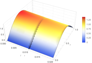
Refer to caption
Figure 1. The uncontrolled solution.
Refer to caption
Figure 2. The controlled solution.

The initial iteration of the algorithm is chosen as 𝐟0=0subscript𝐟00\mathbf{f}_{0}=0. We have chosen ε=104𝜀superscript104\varepsilon=10^{-4} and the stopping parameter tol=103𝑡𝑜𝑙superscript103tol=10^{-3}. The algorithm stops at the iteration number k=25subscript𝑘25k_{*}=25. In Figure 2, we clearly see the effect of the impulse control at time τ=0.01𝜏0.01\tau=0.01.

Refer to caption
Figure 3. The final state for uncontrolled and controlled solutions.

Refer to caption
Figure 4. The computed control hh.

Table 1. Numerical results for T=0.02𝑇0.02T=0.02, τ=0.01𝜏0.01\tau=0.01 and tol=103𝑡𝑜𝑙superscript103tol=10^{-3}.

ε102103104Niter61025Ψ(T)8.54×1027.27×1026.47×102hL2(ω)0.94781.13252.2109missing-subexpressionmissing-subexpressionmissing-subexpressionmissing-subexpressionmissing-subexpressionmissing-subexpressionmissing-subexpressionmissing-subexpression𝜀superscript102superscript103superscript104missing-subexpressionmissing-subexpressionmissing-subexpressionmissing-subexpressionmissing-subexpressionmissing-subexpressionmissing-subexpressionmissing-subexpressionsubscript𝑁iter61025missing-subexpressionmissing-subexpressionmissing-subexpressionmissing-subexpressionmissing-subexpressionmissing-subexpressionmissing-subexpressionmissing-subexpressionnormΨ𝑇8.54superscript1027.27superscript1026.47superscript102missing-subexpressionmissing-subexpressionmissing-subexpressionmissing-subexpressionmissing-subexpressionmissing-subexpressionmissing-subexpressionmissing-subexpressionsubscriptnormsuperscript𝐿2𝜔0.94781.13252.2109missing-subexpressionmissing-subexpressionmissing-subexpressionmissing-subexpression\begin{array}[]{cccc}\hline\cr\\[-8.53581pt] \varepsilon&10^{-2}&10^{-3}&10^{-4}\\ \hline\cr\\[-8.53581pt] N_{\text{iter}}&6&10&25\\ \hline\cr\\[-8.53581pt] \|\Psi(T)\|&8.54\times 10^{-2}&7.27\times 10^{-2}&6.47\times 10^{-2}\\ \hline\cr\\[-8.53581pt] \|h\|_{L^{2}(\omega)}&0.9478&1.1325&2.2109\\ \hline\cr\\[-8.53581pt] \end{array}

We clearly see that the distance Ψ(T)normΨ𝑇\|\Psi(T)\| to the target zero decreases and the norm of the impulse control hL2(ω)subscriptnormsuperscript𝐿2𝜔\|h\|_{L^{2}(\omega)} increases as ε𝜀\varepsilon diminishes.

Remark 5.1.

The above numerical tests show that the proposed algorithm yields accurate and fast results for the numerical computation of distributed impulsive controls controlling the heat equation with dynamic boundary conditions at a single instant of time τ𝜏\tau. This approach can be generalized for more general and multi-dimensional parabolic systems with dynamic boundary conditions.

6. Conclusions and Remarks

In this work, a logarithmic convexity result has been proved for the 1-D heat equation with dynamic boundary conditions. As an application, the impulsive approximate controllability for the system (1.1) has been established with an explicit bound of the cost. The proof is based on the Carleman commutator approach. Afterward, a constructive algorithm has been developed to numerically construct the impulse control of minimal L2superscript𝐿2L^{2}-norm. This has been done by combining a penalized HUM approach and a CG method. Finally, a numerical simulation has been performed to illustrate the theoretical result of impulse approximate controllability.

To the best of the authors knowledge, dynamical systems with impulsive controls have not been much studied numerically, which opens the doors to many possibilities for dealing with such problems. This work can be generalized in several ways, for instance, one would study the case of an infinite number of impulses or the case of some perturbations as: nonlinearities, delays and non local conditions. One would also change the type of impulses by considering non-instantaneous impulses. Such problems would be of much interest to investigate.

Acknowledgment

The authors would like to express their thanks to anonymous referees for constructive comments and suggestions that improved the quality of this manuscript.

References

  • [1] Agarwal,R., Hristova, S. & O’Regan, D. (2017) Non-Instantaneous Impulses in Differential Equations, Springer, Cham.
  • [2] Ait Ben Hassi, E. M., Chorfi, S. E. & Maniar, L. (2021) An inverse problem of radiative potentials and initial temperatures in parabolic equations with dynamic boundary conditions, J. Inverse Ill-Posed Probl,  doi: 10.1515/jiip-2020-0067
  • [3] Ait Ben Hassi, E. M., Chorfi, S. E. & Maniar, L. (2022) Identification of source terms in heat equation with dynamic boundary conditions, Math. Meth. Appl. Sci.,  45, 2364–2379.
  • [4] Ait Ben Hassi, E. M., Chorfi S. E. & Maniar, L. (2021) Inverse problems for general parabolic systems and application to Ornstein-Uhlenbeck equation,   arXiv: 2110.01321.
  • [5] Ait Ben Hassi, E. M., Chorfi S. E., Maniar, L. & Oukdach, O., (2021) Lipschitz stability for an inverse source problem in anisotropic parabolic equations with dynamic boundary conditions, Evol. Equat. and Cont. Theo.,  10, 837–859.
  • [6] Bardos, C. & Phung, K. D., (2017) Observation estimate for kinetic transport equations by diffusion approximation, C. R. Math., 355, 640–664.
  • [7] Ben Aissa, A. & Zouhair, W., (2021) Qualitative properties for the 1D1𝐷1-D impulsive wave equation: controllability and observability, Quaest. Math.,  doi: 10.2989/16073606.2021.1940346.
  • [8] Bensoussan, A., Da Prato, G., Delfour, M. C., & Mitter, S. K. (2007) Representation and control of infinite dimensional systems, Boston, Birkhäuser.
  • [9] Boutaayamou, I., Chorfi S. E., Maniar, L. & Oukdach, O., (2021) The cost of approximate controllability of heat equation with general dynamical boundary conditions, Portugal. Math. 78, 65–99.
  • [10] Boyer. F (2013) On the penalised HUM approach and its applications to the numerical approximation of null-controls for parabolic problems. ESAIM: Proc. 41, 15–58.
  • [11] Buffe, R. & Phung, K. D. (2021) Observation estimate for the heat equations with Neumann boundary condition via logarithmic convexity,  arXiv: arXiv:2105.12977
  • [12] Carrasco, A., Guevara, G., & Leiva, H. (2017) Controllability of the impulsive semilinear beam equation with memory and delay, IMA J. Math. Control. Inf., 36, 213–223.
  • [13] Chorfi, S. E., El. Guermai, G., Maniar, L. & Zouhair, W., (2021) Impulsive null approximate controllability for heat equation with dynamic boundary conditions, submitted.
  • [14] Duque, C., Uzcategui, J., Leiva, H. & Camacho, O. (2013) Approximate controllability of semilinear strongly damped wave equation with impulses, delays, and nonlocal conditions, J. Math. Comput. Sci, 20, 108–121.
  • [15] Fattorini, H. O. & Russell, D. L. (1971) Exact controllability theorems for linear parabolic equations in one space dimension, Arch Ration Mech Anal. 43, 272–292.
  • [16] Glowinski, R., Lions, J.-L. & He, J., (2008) Exact and Approximate Controllability for Distributed Parameter Systems: a Numerical Approach, 117, Encyclopedia of mathematics and its applications, Cambridge University Press, Cambridge, UK; New York.
  • [17] Jose, S. A., Yukunthorn, W., Valdes, J. E. N., & Leiva, H. (2020) Some existence, uniqueness and stability results of nonlocal random impulsive integro-differential equations, Appl. Math. E-Notes, 20, 481–492.
  • [18] Khapalov, A.Y. (1996) Exact controllability of second-order hyperbolic equations with impulse controls, Appl. Anal., 63, 223–238.
  • [19] Khoutaibi, A. (2020) Null controllability of linear and semilinear parabolic equations with dynamic boundary conditions. PhD thesis, Cadi Ayyad University.
  • [20] Khoutaibi, A. & Maniar, L. (2020) Null controllability for a heat equation with dynamic boundary conditions and drift terms, Evol. Equat. and Cont. Theo. 9, 535–559.
  • [21] Kumar, V. & Malik, M. (2021) Controllability results of fractional integro-differential equation with non-instantaneous impulses on time scales, IMA J. Math. Control. Inf. 35, 211–231.
  • [22] Kumpf, M. & Nickel, G. (2004) Dynamic boundary conditions and boundary control for the one-dimensional heat equation, J. Dynam. Control Systems. 10, 213–225.
  • [23] Langer, R. E. (1932) A problem in diffusion or in the flow of heat for a solid in contact with a fluid, Tohoku Math. J. 35, 260–275.
  • [24] Lalvay, S., Padilla-Segarra, A., & Zouhair, W., (2022) On the existence and uniqueness of solutions for non-autonomous semi-linear systems with non-instantaneous impulses, delay, and non-local conditions, Miskolc Math. Notes.
  • [25] Leiva, H., Zouhair, W. & Cabada, D. (2021) Existence, uniqueness and controllability analysis of Benjamin-Bona-Mahony equation with non instantaneous impulses, delay and non local conditions, J. Math. Control. Sci. Appl. 7, 91–108.
  • [26] Li, J. G. & Su, N. (1985) The solution of an infiltration problem with ponded surface flux condition, Acta Math. Appl. Sinica 35, 54–65.
  • [27] Malik, M. & Kumar, A. (2020) Existence and controllability results to second order neutral differential equation with non-instantaneous impulses, J. Control. Decis. 7, 286–308.
  • [28] Maniar, L., Meyries, M., & Schnaubelt, R. (2017) Null controllability for parabolic equations with dynamic boundary conditions, Evol. Equat. and Cont. Theo. 6, 381–407.
  • [29] Milman V. D. & Myshkis, A. D. (1960)On the stability of motion in the presence of impulses, Sibirskii Matematicheskii Zhurnal 1, 233–237.
  • [30] Miller, B. & Rubinovich, E. Y. (2003) Impulsive Control in Continuous and Discrete-Continuous Systems, Springer Verlag, 6.
  • [31] Phung, K. D. (2018) Carleman commutator approach in logarithmic convexity for parabolic equations, Math. Control Rel. Fields, 8, 899–933.
  • [32] Phung, K. D., Wang, G., & Xu, Y. (2017) Impulse output rapid stabilization for heat equations, J Differ. Equ., 263, 5012–5041.
  • [33] Phung, K. D., Wang, L., & Zhang, C. (2014) Bang-bang property for time optimal control for semilinear heat equation, Ann. I. H. Poincare-An., 31, 477–499.
  • [34] Payne, L. E. (2017) Improperly Posed Problems in Partial Differential Equations, SIAM, Philadelphia.
  • [35] Qin, S. & Wang, G. (2017) Controllability of impulse controlled systems of heat equations coupled by constant matrices, J Differ. Equ., 263, 6456–6493.
  • [36] Terzieva, R. (2018) Some phenomena for non-instantaneous impulsive differential equations, Int J Pure Appl. Math., 119, 483–490.
  • [37] Yang, T. (2001) Impulsive Control Theory,Springer Verlag, 227.
  • [38] Zuazua, E. (2007) Controllability and Observability of Partial Differential Equations: some results and open problems, Handbook of differential equations: evolutionary equations, 03, 527-621.