Adversarial Parameter Attack on Deep Neural Networks

Abstract

In this paper, a new parameter perturbation attack on DNNs, called adversarial parameter attack, is proposed, in which small perturbations to the parameters of the DNN are made such that the accuracy of the attacked DNN does not decrease much, but its robustness becomes much lower. The adversarial parameter attack is stronger than previous parameter perturbation attacks in that the attack is more difficult to be recognized by users and the attacked DNN gives a wrong label for any modified sample input with high probability. The existence of adversarial parameters is proved. For a DNN ${\mathcal{F}}_{\Theta}$ with the parameter set $\Theta$ satisfying certain conditions, it is shown that if the depth of the DNN is sufficiently large, then there exists an adversarial parameter set $\Theta_{a}$ for $\Theta$ such that the accuracy of ${\mathcal{F}}_{\Theta_{a}}$ is equal to that of ${\mathcal{F}}_{\Theta}$, but the robustness measure of ${\mathcal{F}}_{\Theta_{a}}$ is smaller than any given bound. An effective training algorithm is given to compute adversarial parameters and numerical experiments are used to demonstrate that the algorithms are effective to produce high quality adversarial parameters.

Keyword. Adversarial parameter attack, adversarial samples, robustness measurement, adversarial accuracy, mathematical theory for safe DNN.

1 Introduction

The deep neural network (DNN) [15] has become the most powerful machine learning method, which has been successfully applied in computer vision, natural language processing, and many other fields. Safety is a key desired feature of DNNs, which was studied extensively [1, 5, 42].

The most widely studied safety issue for DNNs is the adversarial sample attack [31], that is, it is possible to intentionally make small modifications to a sample, which are essentially imperceptible to the human eye, but the DNN outputs a wrong label or even any label given by the adversary. Existence of adversary samples makes the DNN vulnerable in safety-critical applications and many effective methods were proposed to develop more robust DNNs against adversarial attacks [20, 1, 5, 42]. However, it was shown that adversaries samples are inevitable for current DNN models in certain sense [6, 3, 27].

More recently, the parameter perturbation attacks [18, 43, 7, 33, 30, 37, 34, 35] were studied and shown to be another serious safety treat to DNNs. It was shown that by making small parameter perturbations, the attacked DNN can give wrong or desired labels to specified input samples and still give the correct labels to other samples [18, 43, 34, 35].

In this paper, the adversarial parameter attack is proposed, in which small perturbations to the parameters of a DNN are made such that the attack to the DNN is essentially imperceptible to the user, but the robustness of the DNN becomes much lower. The adversarial parameter attack is stronger than previous parameter perturbation attacks in that not only the accuracy but also the robustness of DNNs are considered.

1.1 Contributions

Let ${\mathcal{F}}_{\Theta}$ be a DNN with $\Theta$ as the parameter set. A parameter perturbation $\Theta_{a}$ is called a set of adversarial parameters of $F_{\Theta}$ or $\Theta$, if the following conditions are satisfied 1) $\Theta_{a}$ is a small modification of $\Theta$, for instance $||\Theta_{a}-\Theta||_{\infty}\leq\epsilon$ for a small positive number $\epsilon$; 2) the accuracy of ${\mathcal{F}}_{\Theta_{a}}$ over a distribution of samples is almost the same as that of ${\mathcal{F}}_{\Theta}$; 3) ${\mathcal{F}}_{\Theta_{a}}$ is much less robust than ${\mathcal{F}}_{\Theta}$, that is, ${\mathcal{F}}_{\Theta_{a}}$ has much more adversarial samples than ${\mathcal{F}}_{\Theta}$. It is clear that conditions 1) and 2) are to make the attack difficult to be recognized by the users and condition 3) is to make the new DNN less safe. The DNN obtained by the above attack is called an adversarial DNN, which has high accuracy but low robustness.

The existence of adversarial parameters is proved under certain assumptions. It is shown that if the depth of a trained DNN ${\mathcal{F}}_{\Theta}$ is sufficiently large, then there exist adversarial parameters $\Theta_{a}$ such that the accuracy of ${\mathcal{F}}_{\Theta_{a}}$ is equal to that of ${\mathcal{F}}_{\Theta}$, but the robustness measure of ${\mathcal{F}}_{\Theta_{a}}$ is as small as possible (refer to Corollaries 4.4 and 4.5). Since ${\mathcal{F}}_{\Theta}$ is a continuous function in $\Theta$, if $\Theta_{a}$ is an adversarial parameter for $\Theta$ then there exists a small sphere $S_{a}$ with $\Theta_{a}$ as center such that all parameters in $S_{a}$ are also adversarial parameters for $\Theta$. These results imply that adversarial parameters are inevitable in certain sense, similar to adversarial samples [6, 3, 27].

The existence of adversarial samples is usually demonstrated with numerical experiments, besides a few cases to be mention in the next section. As an application of adversarial parameters, we can construct DNNs which are guaranteed to have adversarial samples. For a trained DNN ${\mathcal{F}}_{\Theta}$ satisfying certain conditions, it is shown that there exist adversarial parameters $\Theta_{a}$ such that the accuracy of ${\mathcal{F}}_{\Theta_{a}}$ is equal to that of ${\mathcal{F}}_{\Theta}$, but ${\mathcal{F}}_{\Theta_{a}}$ has adversarial samples near a given normal sample (refer to Theorem 4.1), or the probability for ${\mathcal{F}}_{\Theta_{a}}$ to have adversarial samples over a distribution of samples is at least $1/2$ (refer to Theorem 4.2).

Finally, an effective training algorithm is given to compute adversarial parameters and numerical experiments are used to demonstrate that the algorithms are effective to produce high quality adversarial parameters for the networks VGG19 and Resnet56 on the CIFAR-10 dataset.

1.2 Related work

There exist vast literatures on adversarial attacks, which can be found in the survey papers [1, 5, 42]. We will focus on those which are closely related to our work.

Parameter perturbation attacks. Parameter perturbation attacks were given under different names such as fault injection attack, fault sneaking attack, stealth attack, and weight corruption. The fault injection attack [18] was first proposed by Liu et al, where it was shown that parameter perturbations can be used to misclassify one given input sample. In [7], it was shown that laser injection techniques can be used as a successful fault injection attack in real-world applications. In [43], the fault sneaking attack was proposed, where multiple input samples were misclassified and other samples were still given the correct label. In [37], lower bounds were given for parameter perturbations under which the network still gives the correct label for a given sample. In [33], upper bounds were given for the changes of the pairwise class margin function and the Rademacher complexity against parameter perturbations and new loss functions were given to obtain more robust networks. In [30], the maximum change of the loss function over given samples was used as an indicator to measure the robustness of DNNs against parameter perturbations and gradient decent methods were used to compute the indicator. In [34, 35], the stealth attack which can guaranteed to make the attacked DNN gives a desired label for a sample outside of the validation set and keep correct labels for samples in the validation set. The stealth attack has the form ${\mathcal{F}}+{\mathcal{U}}$, where ${\mathcal{F}}$ is the DNN to be attacked and ${\mathcal{U}}$ is a DNN with one hidden layer.

The adversarial parameter attack proposed in this paper is stronger than previous parameter perturbation attacks by in the following aspects. First, by keeping the accuracy and eliminating the robustness, the adversarial parameter attack is more difficult to be recognized, because the attached DNN performs almost the same as the original DNN on the test set. Second, by reducing the robustness of the DNN, the attacked DNN gives a wrong label for any modified input sample with high probability, while previous parameter attacks usually misclassify certain given samples. Finally, we prove the existence of adversarial parameters under reasonable assumptions.

Mathematical theories of adversarial samples. Existence of adversarial samples were usually demonstrated with numerical experiments, and mathematical theories were desired. In [6], it was proved that for DNNs with a fixed architecture, there exist uncountable classification functions and distributions of samples such that adversarial samples always exist for any successfully trained DNN with the given architecture and the sample distribution. In the stealth attack [34, 35], it was proved that there exist attached DNNs which give a desired label for a sample outside of the validation set by modifying the DNN. In this paper, we show that by making small perturbations to the parameters of the DNN, the DNN has adversarial samples with high probability.

Theories for certified robustness of DNNs were given in several aspects. Let $x$ be a sample such that the DNN ${\mathcal{F}}$ gives the correct label. Due to the continuity of the DNN function, a sphere with $x$ as center does not contain adversarial samples if its radius is sufficiently small, which is called a robust sphere of $x$. In [12], lower bounds for the robustness radius were computed and used to enhance the robustness of the DNN. In [24], for shallow networks, the upper bounds of the changes of the network under sample input perturbations were given and use to obtain more robust DNNs. In [8], the random smoothing method was proposed and lower bounds for the radius of the robust spheres was given. In [39], lower bounds for the average radius of robust spheres for a distribution of samples are given. Universal lower bounds on stability in terms of the dimension of the domain of the classification function were also given in [27, 34]. However, these bounds are usually inverse-exponentially dependent on the depth of the DNN, which are very small for deep networks in real world applications. In [40], the information-theoretically safe bias classifier was introduced by making the gradient of the DNN random.

Algorithms to train robust DNNs. Many effective methods were proposed to train more robust DNNs to defend adversarial samples [1, 5, 42, 38]. Methods to train DNNs which are more robust against parameter perturbation attacks were also proposed [18, 43]. The adversarial training method proposed by Madry et al [20] can reduce adversarial samples significantly, where the value of the loss function of the worst adversary in a small neighborhood of the training sample is minimized. In this paper, the idea of adversarial training is used to compute adversarial parameters.

2 Adversarial parameters

In this section, we define the adversarial parameters and give a measurement for the quality of the adversarial parameters.

2.1 Adversarial parameters of DNNs

Let us consider a standard DNN. Denote ${\mathbb{I}}=[0,1]\subset{\mathbb{R}}$ and $[n]=\{1,\ldots,n\}$ for $n\in{\mathbb{N}}_{+}$. In this paper, we assume that ${\mathcal{F}}:{\mathbb{I}}^{n}\to{\mathbb{R}}^{m}$ is a classification DNN for $m$ objects, which has $L$ hidden-layers, all hidden-layers use Relu as the activity function, and the output layer does not have activity functions. ${\mathcal{F}}$ can be written as

$$\begin{array}[]{ll}x_{0}\in{\mathbb{I}}^{n},n_{0}=n,n_{L+1}=m;\\ x_{l}={\hbox{\rm{Relu}}}(W_{l}x_{l-1}+b_{l})\in{\mathbb{R}}^{n_{l}},W_{l}\in{\mathbb{R}}^{n_{l}\times n_{l-1}},b_{l}\in{\mathbb{R}}^{n_{l}},l\in[L];\\ {\mathcal{F}}(x_{0})=x_{L+1}=W_{L+1}x_{L}+b_{L+1},W_{L+1}\in{\mathbb{R}}^{m\times n_{L}},b_{L+1}\in{\mathbb{R}}^{m}.\\ \end{array}$$ (1)

Denote $\Theta=\{W_{l},b_{l}\}_{l=1}^{L+1}\in{\mathbb{R}}^{k}$ to be the parameter set of ${\mathcal{F}}$ and ${\mathcal{F}}$ is denoted as ${\mathcal{F}}_{\Theta}$ if the parameters need to be mentioned explicitly, where $k=\sum_{l=1}^{L+1}n_{l}(n_{l-1}+1)$.

Let ${\mathcal{F}}_{\Theta}$ be a trained network with the parameter set $\Theta$. Then a new parameter set $\Theta_{a}$ is called a set of adversarial parameters of $\Theta$ if 1) $\Theta_{a}$ is a small perturbation of $\Theta$; 2) the accuracy of ${\mathcal{F}}_{\Theta_{a}}$ is almost the same as that of ${\mathcal{F}}_{\Theta}$; 3) ${\mathcal{F}}_{\Theta_{a}}$ is much less robust comparing to ${\mathcal{F}}_{\Theta}$, that is, ${\mathcal{F}}_{\Theta_{a}}$ has more adversarial samples than ${\mathcal{F}}_{\Theta}$.

We assume that the objects to be classified satisfy a distribution $D_{x}$ in ${\mathbb{R}}^{n}$, and a sample $x\sim D_{x}$ is called a normal sample. Let $\Theta\in{\mathbb{R}}^{k}$ be the parameter set of a trained network ${\mathcal{F}}_{\Theta}:{\mathbb{I}}^{n}\to{\mathbb{R}}^{m}$. For $x\sim D_{x}$, denote $l_{x}$ to be the label of $x$ and $\widehat{{\mathcal{F}}}_{\Theta}$ to be the classification result of ${\mathcal{F}}_{\Theta}$. Then the accuracy of ${\mathcal{F}}_{\Theta}$ for the normal samples is

$$A({\mathcal{F}}_{\Theta},D_{x})=P_{x\sim D_{x}}(\widehat{{\mathcal{F}}}_{\Theta}(x)=l_{x}).$$ (2)

In order to measure the quality of adversarial parameters, we need a robustness measure $R({\mathcal{F}}_{\Theta},D_{x})$ of ${\mathcal{F}}_{\Theta}$ for the normal samples. There exist several definitions for $R({\mathcal{F}}_{\Theta},D_{x})$ [20, 39]. In this paper, two kinds of robustness measures are used.

We first give two robust measures of ${\mathcal{F}}_{\Theta}$ on a given sample $x_{0}$. The robustness radius of $x_{0}$ under the $L_{p}$ norm for $p\in{\mathbb{R}}_{+}\cup\{\infty\}$ is defined to be

$$R_{1}({\mathcal{F}}_{\Theta},x_{0})=\max\{\zeta\in{\mathbb{R}}_{+}\,|\,\widehat{{\mathcal{F}}}(x)=l_{x},\forall x\hbox{ s.t. }||x-x_{0}||_{p}\leq\zeta\}.$$ (3)

If $\widehat{{\mathcal{F}}}_{\Theta}(x_{0})\neq l_{x_{0}}$, then the robustness radius of $x_{0}$ is zero. It is difficult to have good estimation to the robustness radius, and the following approximation to the robust radius under $L_{p}$ norm [12] is often used

$$R_{2}({\mathcal{F}}_{\Theta},x_{0})=\min_{l\in[m],l\neq l_{x}}\{\frac{|{\mathcal{F}}_{l_{x}}(x_{0})-{\mathcal{F}}_{l}(x_{0})|}{||\nabla{\mathcal{F}}_{l_{x}}(x_{0})-\nabla{\mathcal{F}}_{l}(x_{0})||_{q}}I({\mathcal{F}}_{l_{x}}(x_{0})>{\mathcal{F}}_{l}(x_{0}))\}$$ (4)

where ${\mathcal{F}}_{l}(x_{0})$ is the $l$-th coordinate of ${\mathcal{F}}(x_{0})$, $\nabla({\mathcal{F}}_{l}(x))=\frac{\nabla{\mathcal{F}}_{l}(t)}{\nabla t}|_{t=x}$, $p,q\in{\mathbb{R}}_{+}\{\infty\}$ satisfy $1/q+1/p=1$ ($p=0(\infty)$ iff $q=\infty(0)$), and $I(t)=1$ if $t$ it true or $I(t)=0$ otherwise.

For a distribution $D_{x}$ of samples, we define two global robust measures corresponding to $R_{1}$ and $R_{2}$. The adversarial accuracy can be used as $R({\mathcal{F}}_{\Theta},D_{x})$. For $\epsilon\in{\mathbb{R}}_{+}$ and $p\in{\mathbb{R}}_{+}\cup\{\infty\}$, the adversarial accuracy of ${\mathcal{F}}_{\Theta}$ is

$$\begin{array}[]{ll}R_{3}({\mathcal{F}}_{\Theta},D_{x},\epsilon)&=P_{x\sim D_{x}}(\epsilon\leq R_{1}({\mathcal{F}}_{\Theta},x))\\ &=P_{x\sim D_{x}}(\widehat{{\mathcal{F}}}_{\Theta}(x^{\prime})=l_{x},\forall x^{\prime}\hbox{ s.t. }||x^{\prime}-x||_{p}\leq\epsilon).\end{array}$$ (5)

Corresponding to $R_{2}$ in (4), we have the following global robustness measure

$$R_{4}({\mathcal{F}},D_{x})=\int_{x\sim D_{x}}R_{2}({\mathcal{F}},x){\hbox{\rm{d}}}x.$$ (6)

We now define a measurement for an adversarial parameter set using the accuracy and robustness of ${\mathcal{F}}$.

Definition 2.1.

Let $\Theta_{a}$ be an adversarial parameter set of $\Theta$, $R({\mathcal{F}},D_{x})$ a robustness measure of ${\mathcal{F}}$ for normal samples, and

$$P_{x\sim D_{x}}({{\mathcal{F}}}_{\Theta_{a}}(x)=l_{x})=\gamma_{1}P_{x\sim D_{x}}({{\mathcal{F}}}_{\Theta}(x)=l_{x})$$ (7)

$$R({\mathcal{F}}_{\Theta_{a}},D_{x})=\gamma_{2}R({\mathcal{F}}_{\Theta},D_{x}).$$

Then the adversarial rate of $\Theta_{a}$ is defined to be $\overline{\gamma_{1}}(1-\overline{\gamma_{2}})$, where $\overline{\gamma}=\min\{\gamma,1\}$.

In general, we have $\gamma_{1}\leq 1$ and $\gamma_{2}\leq 1$. The value of $\gamma_{1}$ measures the ability of $\Theta_{a}$ to keep the accuracy of ${\mathcal{F}}_{\Theta}$ on normal samples, and if $\gamma_{1}$ is large then the attack is more difficult to be detected. The value of $1-\gamma_{2}$ measures the ability of $\Theta_{a}$ to break the robustness of ${\mathcal{F}}_{\Theta}$, and if $1-\gamma_{2}$ is large then the parameter attack is more powerful. Hence, the adversarial rate $\overline{\gamma_{1}}(1-\overline{\gamma_{2}})$ measures the quality of the adversarial parameter attack in that if the adversarial rate is larger then the adversarial parameter attack is better. If $\overline{\gamma_{1}}(1-\overline{\gamma_{2}})$ achieves its maximal value $1$, then $\gamma_{1}=1$ and $\gamma_{2}=0$ and the adversarial parameter attack is a perfect attack in that the attack does not change the accuracy of ${\mathcal{F}}$, but totally destroys the robustness of ${\mathcal{F}}$.

Remark 2.1.

In order to make the attack very hard to be detected, we can give a lower bound $\gamma_{\rm{low}}$ to $\gamma_{1}$. If $\gamma_{1}<\gamma_{\rm{low}}$, we consider $\Theta_{a}$ to be a failed attack.

2.2 Adversarial parameter attacks for other purposes

According to the requirements of specific applications, we may define other types of adversarial parameter attacks.

The adversarial parameters defined in section 2.1 are for all the samples. In certain applications, it is desired to make the network less robust on one specific class of samples, which motivates the following definitions.

The simplest case is adversarial parameters for a given sample. A small perturbation $\Theta_{a}$ of $\Theta$ is called adversarial parameters for a given sample $x_{0}$, if ${\mathcal{F}}_{\Theta_{a}}$ gives the correct label to $x_{0}$ and has adversarial samples of $x_{0}$ in $S_{\infty}(x_{0},\epsilon)=\{x\,|\,|x-x_{0}|_{\infty}\leq\epsilon\}$ for a given $\epsilon\in{\mathbb{R}}_{+}$. Let $R({\mathcal{F}}_{\Theta},x_{0})$ be a measure of robustness of ${\mathcal{F}}_{\Theta}$ at sample $x_{0}$, and

$$R({\mathcal{F}}_{\Theta_{a}},x_{0})=\gamma R({\mathcal{F}}_{\Theta},x_{0}).$$ (8)

Then the adversarial rate of $\Theta_{a}$ is defined to be $1-\overline{\gamma}$.

We can also break the stability for samples with a given label. A small perturbation $\Theta_{a}$ of $\Theta$ is called adversarial parameters for samples with a given label $l_{0}$, if ${\mathcal{F}}_{\Theta_{a}}$ keeps the accuracy for all normal samples and the robustness for normal samples whose label is not $l_{0}$, but break the robustness of samples with label $l_{0}$. Let $\alpha=P_{x\sim D_{x}}(\widehat{{\mathcal{F}}}_{\Theta}(x)=l_{x})$ and $\beta=P_{x\sim D_{x}}(\widehat{{\mathcal{F}}}_{\Theta}(x^{\prime})=l_{x},\forall x^{\prime}\in S_{p}(x,\epsilon))$. For such adversarial parameters $\Theta_{a}$, let

$$P_{x\sim D_{x}}(\widehat{{\mathcal{F}}}_{\Theta_{a}}(x)=l_{x})=\gamma_{1}\alpha$$ (9)

$$P_{x\sim D_{x}}(\widehat{{\mathcal{F}}}_{\Theta_{a}}(x^{\prime})=l_{x},\forall x^{\prime}\in B_{p}(x,\epsilon)\,|\,l_{x}\neq y_{0})=\gamma_{2}\beta$$

$$P_{x\sim D_{x}}(\widehat{{\mathcal{F}}}_{\Theta_{a}}(x^{\prime})=l_{x},\forall x^{\prime}\in B_{p}(x,\epsilon)\,|\,l_{x}=y_{0})=\gamma_{3}\beta.$$

Then the adversarial rate of $\Theta_{a}$ is defined as $\overline{\gamma}_{1}\overline{\gamma}_{2}(1-\overline{\gamma}_{3})$.

Finally, instead of breaking the robustness of samples with label $y_{0}$, we can break the accuracies for samples with label $y_{0}$. Such adversarial parameters are called direct adversarial parameters. Let $\Theta_{a}$ be a direct adversarial parameter set and

$$P_{x\sim D_{x}}(\widehat{{\mathcal{F}}}_{\Theta_{a}}(x)=l_{x}\,|\,l_{x}\neq y_{0})=\gamma_{1}\alpha$$ (10)

$$P_{x\sim D_{x}}(\widehat{{\mathcal{F}}}_{\Theta_{a}}(x^{\prime})=l_{x},\forall x^{\prime}\in B_{p}(x,\epsilon)\,|\,l_{x}\neq y_{0})=\gamma_{2}\beta$$

$$P_{x\sim D_{x}}(\widehat{{\mathcal{F}}}_{\Theta_{a}}(x)=l_{x}\,|\,l_{x}=y_{0})=\gamma_{3}\alpha.$$

Then the adversarial rate is defined as $\overline{\gamma}_{1}\overline{\gamma}_{2}(1-\overline{\gamma}_{3})$. The above definition is similar to the attacks in [18, 43], but robustness is considered as an extra objective.

3 Algorithm

In this section, we give algorithms to compute adversarial parameters.

3.1 Compute adversarial parameters under $L_{\infty}$ norm

We formulate the adversarial parameter attack for a trained DNN ${\mathcal{F}}_{\Theta}$ under the $L_{p}$ norm as the following optimization problem for a given $\zeta\in{\mathbb{R}}_{+}$.

$$\max_{\Theta_{a}\in{\mathbb{R}}^{k},||\Theta_{a}-\Theta||_{p}\leq\zeta}A({\mathcal{F}}_{\Theta_{a}},D_{x})/R({\mathcal{F}}_{\Theta_{a}},D_{x})$$ (11)

where $A({\mathcal{F}}_{\Theta_{a}},D_{x})$ and $R({\mathcal{F}}_{\Theta_{a}},D_{x})$ are the accuracy and a robustness measure for ${\mathcal{F}}_{\Theta_{a}}$ over a distribution sample $D_{x}$.

Remark 3.1.

Theoretically, the adversarial parameter attack should be a multi-objective optimization problem, that is to maximize the accuracy and to minimize the robustness. But, such an optimization problem is difficult to solve.

Remark 3.2.

According to (11), the adversarial rate seems better to be defined as $\gamma_{1}/\gamma_{2}$, which is possible but not as good as the one in Definition 2.1 for the following reasons. The adversarial rate $\overline{\gamma_{1}}(1-\overline{\gamma_{2}})$ has the optimal value $1$ and gives a more intuitive view to see the quality of the adversarial parameters.

In the rest of this section, we show how to change formula (11) to an effective algorithm to compute $L_{\infty}$ norm adversarial parameters using the robustness measure in (5). We first show how to compute the robustness in (5) explicitly. We use the adversarial training [20] to do that, which is the most effective way to find adversarial samples. For a sample $x$ and a small number $\varepsilon\in{\mathbb{R}}_{+}$, we first compute

$$\chi_{0}={\arg\max}_{\chi\in{\mathbb{R}}^{k},||\chi||_{0}<\varepsilon}L_{{\hbox{\scriptsize\rm{CE}}}}({\mathcal{F}}_{\Theta}(x+\chi),l_{x})$$

with PGD [20] and then use

$$L_{{\hbox{\scriptsize\rm{AT}}}}(x,\Theta)=L_{{\hbox{\scriptsize\rm{CE}}}}({\mathcal{F}}_{\Theta}(x+\chi_{0}),l_{x})$$ (12)

to measure the robustness of ${\mathcal{F}}_{\Theta}$ at $x$.

We need a training set $T$ to find the adversarial parameters. The training procedure consists of two phases. In the first pre-training phase, the loss function

$$-\sum_{x\in T}L_{{\hbox{\scriptsize\rm{AT}}}}(x,\Theta)$$ (13)

is used to reduce the adversarial accuracy of ${\mathcal{F}}_{\Theta}$. In the second main training phase, the loss function

$$\frac{\sum_{x\in T}L_{{\hbox{\scriptsize\rm{CE}}}}({\mathcal{F}}_{\Theta}(x),l_{x})}{\sum_{x\in T}L_{{\hbox{\scriptsize\rm{AT}}}}(x,\Theta)}$$ (14)

is used to promote the accuracy and keep the low-level of adversarial accuracy of ${\mathcal{F}}_{\Theta}$, which corresponds to formula (11).

We will compute a more general $L_{\infty}$ norm parameter perturbation. Let $\Delta\in{\mathbb{R}}_{+}^{k}$ and $\Delta_{i}$ the $i$-th coordinate of $\Delta$. Then the $L_{\infty}$ parameter perturbation will be found in

$$B_{\infty}(\Theta,\Delta)=\{\Theta_{a}\in{\mathbb{R}}^{k}\,|\,|\Theta_{a}-\Theta|_{i}\leq\Delta_{i},\ \forall\ i\in[k]\}.$$

It is clear that the usual $L_{\infty}$ norm parameter perturbation is a special case of the above general case. We use this general form, because we want to include more types of parameter perturbations which are given in section 5.2. A sketch of the algorithm is given below.

Algorithm 1 Attack under $L_{\infty}$ norm

0:    The parameter set $\Theta$ of ${\mathcal{F}}$;The hyper-parameters: $\alpha\in{\mathbb{R}}_{+}$, $\Delta\in{\mathbb{R}}_{+}^{k}$, $n_{1},n_{2}\in{\mathbb{N}}$;A training set $T$.

0:  An adversarial parameter set $\Theta_{a}$ in $B_{\infty}(\Theta,\Delta)$.Let $i=0$, $\Theta_{a}=\Theta$.For all $i\in[n_{1}+n_{2}]$: If $i<n_{1}$:  $L=-\sum_{x\in T}\frac{1}{|T|}L_{{\hbox{\scriptsize\rm{AT}}}}(x,\Theta_{a})$. Else:  $L=\frac{\sum_{x\in T}L_{{\hbox{\scriptsize\rm{CE}}}}({\mathcal{F}}_{\Theta_{a}}(x),l_{x})}{\sum_{x\in T}L_{{\hbox{\scriptsize\rm{AT}}}}(x,\Theta_{a})}$. $\widetilde{\Theta}=\Theta_{a}+\alpha\bigtriangledown L$. $\Theta_{a}={\hbox{\rm{Proj}}}(\widetilde{\Theta},B_{\infty}(\Theta,\Delta))$.Output: $\Theta_{a}$.

Remark 3.3.

We give more details for the algorithm.

(1). ${\hbox{\rm{Proj}}}(\widetilde{\Theta},B_{\infty}(\Theta,\Delta))$ maps $\widetilde{\Theta}$ into $B_{\infty}(\Theta,\Delta)$ as follows: for $i\in[k]$:

If $\widetilde{\Theta}_{i}>\Theta_{i}+\Delta_{i}$, ${\hbox{\rm{Proj}}}(\widetilde{\Theta},B_{\infty}(\Theta,\Delta))_{i}=\Theta_{i}+\Delta_{i}$;

If $\widetilde{\Theta}_{i}<\Theta_{i}-\Delta_{i}$, ${\hbox{\rm{Proj}}}(\widetilde{\Theta},B_{\infty}(\Theta,\Delta))_{i}=\Theta_{i}-\Delta_{i}$;

If $\widetilde{\Theta}_{i}+\Delta_{i}>\Theta_{i}>\widetilde{\Theta}_{i}-\Delta_{i}$, ${\hbox{\rm{Proj}}}(\widetilde{\Theta},B_{\infty}(\Theta,\Delta))_{i}=\Theta_{i}$.

(2). We will reduce the training steps $\alpha$ with the training going.

3.2 Algorithms for other kinds of adversarial parameters

The algorithm to find adversarial parameters under other norms and robustness measures can be developed similarly. In what below, we show how to compute adversarial parameters under $L_{0}$ norm, which is different from other cases. The overall algorithm is similar to Algorithm 1, except we use a new method to update the parameters. Suppose that $\Theta=\{W_{l},b_{l}\}_{l=1}^{L}$ is the parameter to be updated and the value of $L$ in Algorithm 1 is found. We will show how to update the parameters. We only change some weight matrices $W_{l}$ as follows.

• Randomly select two entries $w_{1}$ and $w_{2}$ of $W_{l}$ until $(\frac{\nabla L}{\nabla w_{1}}-\frac{\nabla L}{\nabla w_{2}})(w_{1}-w_{2})>0$ is satisfied.

• Exchange $w_{1}$ and $w_{2}$ in $W_{l}$ to obtain the new parameters.

It is clear that the change will make $L$ become smaller. In total, we update a given number of weight matrices, and for each such matrix, we change a given percentage of its entries. The details of the algorithm are omitted. Note that the above parameter perturbation keeps the sparsity and the values of the entries of the weight matrices. As a consequence the Proj operator in the algorithm can be taken as the identity map.

The adversarial parameters defined in section 2.2 can also be obtained similarly. For instance, to compute the adversarial parameters for one sample $x$, we just need to let $T$ in Algorithm 1 to be $T=\{x\}$.

To compute adversarial parameters for samples with a given label $l_{0}$, by (9) we can use the following loss function

$$\frac{\sum_{x\in T}L_{{\hbox{\scriptsize\rm{CE}}}}({\mathcal{F}}_{\Theta_{a}}(x),l_{x})+\sum_{x\in T\ \&\ l_{x}\neq l_{0}}L_{{\hbox{\scriptsize\rm{AT}}}}(x,\Theta_{a})}{\sum_{x\in T\ \&\ l_{x}=l_{0}}L_{{\hbox{\scriptsize\rm{AT}}}}({\mathcal{F}}_{\Theta_{a}}(x),l_{x})}$$ (15)

to increase the robustness and accuracy of samples whose labels are not $l_{0}$ and to reduce the accuracy for samples with labels $l_{0}$.

To compute direct adversarial parameters for samples with label $l_{0}$, by (10) we can use the following loss function

$$\frac{\sum_{x\in T\ \&\ l_{x}\neq l_{0}}(L_{{\hbox{\scriptsize\rm{AT}}}}(x,\Theta_{a})+L_{{\hbox{\scriptsize\rm{CE}}}}({\mathcal{F}}_{\Theta_{a}}(x),l_{x}))}{\sum_{x\in T\ \&\ l_{x}=l_{0}}L_{{\hbox{\scriptsize\rm{CE}}}}({\mathcal{F}}_{\Theta_{a}}(x),l_{x})}$$ (16)

to increase the robustness and accuracy of samples whose labels are not $l_{0}$ and to reduce the accuracy for samples with labels $l_{0}$.

4 Existence of adversarial parameters

In this section, we will show that adversarial parameters with high adversarial rates exist under certain conditions.

4.1 Adversarial parameters to achieve low adversary accuracy

In this section, we use the robustness radius in (3) and the adversarial accuracy in (5) as the robust measures, and hence existence of adversarial parameters implies low adversary accuracies.

We introduce several notations. Let $||x||_{-\infty}=\min_{i\in[n]}\{|x_{i}|\}$ for $x\in{\mathbb{R}}^{n}$, and $||W||_{-\infty,2}=\min_{i\in[a]}\{||W^{(i)}||_{2}\}$ for $W\in{\mathbb{R}}^{a\times b}$, where $W^{(i)}$ is the $i$-th row of $W$. If ${\mathcal{F}}$ is a network, we use ${\mathcal{F}}_{i}(x)$ to denote the $i$-th coordinate of ${\mathcal{F}}(x)$.

In this section, we consider the following network ${\mathcal{F}}_{\Theta}:{\mathbb{I}}^{n}\to{\mathbb{R}}^{m}$ with one hidden layer

$$\begin{array}[]{ll}{\mathcal{F}}(x)=W_{2}{\hbox{\rm{Relu}}}(W_{1}x+b_{1})+b_{2},\end{array}$$ (17)

where $W_{1}\in{\mathbb{R}}^{n_{1}\times n},b_{1}\in{\mathbb{R}}^{n_{1}},W_{2}\in{\mathbb{R}}^{m\times n_{1}},b_{2}\in{\mathbb{R}}^{m}$. $\Theta=\{W_{i},b_{i}\}_{i=1}^{2}\in{\mathbb{R}}^{k}$ is the parameter set of ${\mathcal{F}}_{\Theta}$, where $k=(n+m+1)n_{1}+m$.

The network defined in (17) has just one hidden-layer. We will show that when the width of its hidden-layer is large enough, adversarial parameters exist under with certain conditions.

We will consider $L_{\infty}$ adversarial parameters. For $\gamma\in{\mathbb{R}}_{+}$, the hypothetical space for the adversarial networks of ${\mathcal{F}}_{\Theta}$ is

$${\mathcal{H}}_{\gamma}(\Theta)=\{{\mathcal{F}}_{\Theta_{a}}\,|\,||\Theta_{a}-\Theta||_{\infty}<\gamma\}.$$

The following theorem shows the existence of adversarial parameters for a given sample $x_{0}$. The proof of the theorem is given in section 6.1.

Theorem 4.1.

Let ${\mathcal{F}}_{\Theta}$ be a trained network with structure in (17), which gives the correct label $l_{x_{0}}$ for a sample $x_{0}$. Further assume the following conditions.

$C_{1}$.

Let $a,A\in{\mathbb{R}}_{+}$ such that $|{\mathcal{F}}_{i}(x)-{\mathcal{F}}_{j}(x)|<A$ for all $i,j\in[m]$ and $x\in S_{\infty}(x_{0},a)=\{x\,|\,||x-x_{0}||_{\infty}\leq a\}$.

$C_{2}$.

$||W_{2}^{(i)}-W_{2}^{(j)}||_{-\infty}>c$ for all $i,j\in[m]$, $i\neq j$.

$C_{3}$.

At least $\eta n_{1}$ coordinates of $|{\hbox{\rm{Relu}}}(W_{1}x+b_{1})|$ are bigger than $b$, where $\eta\in(0,1)$ and $b\in{\mathbb{R}}_{+}$.

For $\gamma,\epsilon\in{\mathbb{R}}_{+}$ such that $\epsilon<a$, if $n_{1}>\frac{2A}{\min\{\epsilon\gamma(n-1),b\}c\eta}$, then there exists an ${\mathcal{F}}_{\Theta_{a}}\in{\mathcal{H}}_{\gamma}(\Theta)$ such that $\widehat{{\mathcal{F}}}_{\Theta_{a}}(x_{0})=l_{x_{0}}$ and ${\mathcal{F}}_{\Theta_{a}}$ has adversarial samples to $x_{0}$ in $S_{\infty}(x_{0},\epsilon)$.

We have the following observations from Theorem 4.1.

Corollary 4.1.

If the robustness radius in (3) is used as the robustness measure, then the adversarial rate of ${\mathcal{F}}_{\Theta_{a}}$ in Theorem 4.1 is bigger than $1-\frac{\epsilon}{a}$.

Remark 4.1.

From Theorem 4.1, if the width of ${\mathcal{F}}_{\Theta}$ is sufficiently large, then ${\mathcal{F}}_{\Theta}$ has adversarial parameters which is as close as possible to $\Theta$ and ${\mathcal{F}}_{\Theta_{a}}$ has adversarial samples which are as close as possible to $x_{0}$.

Remark 4.2.

Since ${\mathcal{F}}_{\Theta}$ is a continuous function in $\Theta$, if $\Theta_{a}$ is an adversarial parameter set for $\Theta$ then there exists a small sphere $S_{a}$ with $\Theta_{a}$ as center such that all parameters in $S_{a}$ are also adversarial parameters for $\Theta$.

From the above two remarks, we may say that adversarial parameters are inevitable in this case.

The following theorem shows that when $n_{1}$ is large enough, adversarial parameters exist for a distributions with high probability. The proof of the theorem is given in section 6.1.

Theorem 4.2.

Let ${\mathcal{F}}_{\Theta}$ be a trained DNN with structure in (17) and $S\subset{\mathbb{I}}^{n}$ the set of normal samples. Further assume the following conditions.

$C_{1}$.

Let $A,a\in{\mathbb{R}}_{+}$ such that $|{\mathcal{F}}_{i}(x)-{\mathcal{F}}_{j}(x)|<A$ for all $i,j\in[m]$ and $x\in\bigcup_{x_{0}\in S}S_{\infty}(x_{0},a)$.

$C_{2}$.

$||W_{2}^{(i)}-W_{2}^{(j)}||_{-\infty}>c$ for all $i,j\in[m]$, $i\neq j$, where $c\in{\mathbb{R}}_{+}$.

$C_{3}$.

For all $x\in S$, at least $\eta n_{1}$ coordinates of $|{\hbox{\rm{Relu}}}(W_{1}x+b_{1})|$ are bigger than $b$, where $\eta\in(0,1)$ $b\in{\mathbb{R}}_{+}$.

$C_{4}$.

The dimension of $S$ is lower than $n-m$.

For $\epsilon,\gamma\in{\mathbb{R}}_{+}$ such that $\epsilon<a$, if $n_{1}>\frac{2A}{\min\{\epsilon\gamma/m,b\}c\eta}$, then there exists an ${\mathcal{F}}_{\Theta_{a}}\in{\mathcal{H}}_{\gamma}(\Theta)$ such that the accuracy of ${{\mathcal{F}}}_{\Theta_{a}}$ over $D_{x}$ is greater than or equal to that of ${{\mathcal{F}}}_{\Theta}$ and

$$P_{x\sim D_{x}}({{\mathcal{F}}}_{\Theta_{a}}\ has\ an\ adversarial\ sample\ of\ x\ in\ S_{\infty}(x_{,}\epsilon))\geq 0.5.$$

Corollary 4.2.

Let the adversary accuracy of ${\mathcal{F}}_{\Theta}$ be $\theta=R_{3}({\mathcal{F}}_{\Theta},D_{x},\epsilon)$, then Theorem 4.2 implies that there exists adversarial parameters $\Theta_{a}$ of $\Theta$ with adversarial rate at least $1-0.5/\theta$.

Remark 4.3.

The conditions of Theorems 4.1 and 4.2 can be satisfied for most DNNs. The parameters $A$ and $a$ in Condition $C_{1}$ are clearly exist. Since the training procedure usually terminates near a local minimum of the loss function, the weights can be considered as random values [39], and hence conditions $C_{2}$ and $C_{3}$ can be satisfied. For practical examples such as MNIST and CIFAR-10, condition $C_{4}$ is clearly satisfied.

4.2 Adversarial parameters for DNNs

In this section, we consider networks of the following form

$$\begin{array}[]{ll}x_{0}\in{\mathbb{I}}^{n},n_{L+1}=m;\\ x_{l}={\hbox{\rm{Relu}}}(W_{l}x_{l-1})\in{\mathbb{R}}^{n},W_{l}\in{\mathbb{R}}^{n\times n},l\in[L];\\ {\mathcal{F}}(x_{0})=x_{L+1}=W_{L+1}x_{L}\in{\mathbb{R}}^{m},W_{L+1}\in{\mathbb{R}}^{m\times n}.\\ \end{array}$$ (18)

Let $\Theta=\{W_{i}\}_{i=1}^{L+1}$ be the parameters and $\Theta\in{\mathbb{R}}^{k}$, where $k=Ln^{2}+mn$. We use ${\mathcal{F}}^{l}_{\Theta}(x)$ to represent the output of the $l$-th layer of ${\mathcal{F}}_{\Theta}(x)$ where $l\in[L]$. We will show that, when $L$ becomes big, adversarial parameters exist.

We first prove the existence of adversarial parameters for a given sample. We use the following robustness measure for network ${\mathcal{F}}$ at a sample $x$

$$R({\mathcal{F}},x)=\min_{l\neq l_{x}}\{\frac{|{\mathcal{F}}_{l_{x}}(x)-{\mathcal{F}}_{l}(x)|^{2}}{||\nabla({\mathcal{F}}_{l_{x}}(x))-\nabla({\mathcal{F}}_{l}(x))||_{2}^{2}}I({\mathcal{F}}_{l_{x}}(x)>{\mathcal{F}}_{l}(x))\}.$$

It is easy to see that this is the square of $R_{2}({\mathcal{F}},x)$ in (4) with $p=2$.

Theorem 4.3.

Let ${\mathcal{F}}_{\Theta}$ be a trained network with structure in (18), which gives the correct label for a sample $x_{0}\in{\mathbb{R}}^{n}$. Further assume the following conditions.

$C_{1}$.

$||\frac{\nabla{\mathcal{F}}_{i}(t)}{\nabla t}|_{t=x_{0}}||_{2}<\sqrt{A}$ for $i\in[m]$.

$C_{2}$.

$||\frac{\nabla{\mathcal{F}}^{l}(t)}{\nabla t}|_{t=x_{0}}||_{-\infty,2}>b$ for $l\in[L]$.

$C_{3}$.

$||\frac{\nabla{\mathcal{F}}_{i}(t)-\nabla{\mathcal{F}}_{j}(t)}{\nabla{\mathcal{F}}^{l}(t)}|_{t=x_{0}}||_{-\infty}>c$ for $i,j\in[m]$, $i\neq j$ and $l\in[L]$.

$C_{4}$.

For $l\in[L]$, $\frac{\nabla{\mathcal{F}}^{l}(t)}{\nabla t}|_{t=x_{0}}$ has a column $L_{l}$ such that the angle between $L_{l}$ and ${\mathcal{F}}^{l}(x_{0})$ is bigger than $\alpha$ and smaller than $\pi-\alpha$, where $\alpha\in[0,\pi/2]$.

Then for $\gamma\in{\mathbb{R}}_{+}$, there exists an ${\mathcal{F}}_{\Theta_{a}}\in{\mathcal{H}}_{\gamma}(\Theta)$ such that ${\mathcal{F}}_{\Theta_{a}}(x_{0})=l_{x_{0}}$ and

$$R({\mathcal{F}}_{\Theta_{a}},x_{0})\leq(1-\eta)R({\mathcal{F}}_{\Theta},x_{0})$$

where $\eta=\frac{\gamma^{2}((L-1)(\sin(r)cb)^{2}+c^{2}+(2\sin(r)b)^{2})}{4A+\gamma^{2}((L-1)(\sin(r)cb)^{2}+c^{2}+(2\sin(r)b)^{2})}$. In other words, there exists an ${\mathcal{F}}_{\Theta_{a}}$ with adversarial rate $\geq\eta$.

The proof of the theorem is given in section 6.2. As a consequence of Theorem 4.3, there exist adversarial parameters for sample $x_{0}$, whose robustness measure is as small as possible.

Corollary 4.3.

For $\rho\in(0,1)$, if $L\geq\frac{4(1-\rho)A}{\rho(\gamma\sin(r)cb)^{2}}+1$, then the adversarial rate of ${\mathcal{F}}_{\Theta_{a}}$ is $\geq 1-\rho$.

Corollary 4.4.

For $\tau\in(0,1)$ satisfying $\tau<R({\mathcal{F}},x_{0})$, if $L>\frac{4A(R({\mathcal{F}},x_{0})/\tau-1)}{(\gamma\sin(r)cb)^{2}}+1$, then $R({\mathcal{F}}_{\Theta_{a}},x_{0})\leq\tau$.

To find adversarial parameters for samples under a distribution $D_{x}$, we use the following robustness measure for ${\mathcal{F}}$:

$$R({\mathcal{F}},D_{x})=\frac{\int_{x\sim D_{x}}\min_{j\neq l_{x}}\{||{\mathcal{F}}_{l_{x}}(x)-{\mathcal{F}}_{j}(x)||_{2}^{2}\,I({\mathcal{F}}_{l_{x}}(x)>{\mathcal{F}}_{j}(x))\}{\hbox{\rm{d}}}x}{\int_{x\sim D_{x}}\max_{j\neq l_{x}}\{||\nabla{\mathcal{F}}_{l_{x}}(x)-\nabla{\mathcal{F}}_{j}(x)||_{2}^{2}\}{\hbox{\rm{d}}}x}.$$

This is a variant of $R_{4}({\mathcal{F}},D_{x})$ in (6) with $p=2$. The following theorem shows that adversarial parameters exist for this robustness measure. The proof of the theorem is given in section 6.2.

Theorem 4.4.

Let ${\mathcal{F}}_{\Theta}$ be a trained DNN with structure in (17) and $S\subset{\mathbb{I}}^{n}$ the set of normal samples satisfying distribution $D_{x}$. Further assume the following conditions.

$C_{1}$.

$||\frac{\nabla{\mathcal{F}}_{i}(t)}{\nabla t}|_{t=x}||_{2}<\sqrt{A}$ for all samples $x\in S$ and $i\in[m]$.

$C_{2}$.

$P_{x\sim D_{x}}(\forall l\neq l_{x},\ ||\frac{\nabla({\mathcal{F}}_{l}(t)-{\mathcal{F}}_{l_{x}}(t))}{\nabla{\mathcal{F}}^{l}(t)}|_{t=x}||_{-\infty}>c_{l})>\alpha_{l}$, where $l\in[L]$ and $c_{l},\alpha_{l}\in{\mathbb{R}}_{+}$.

$C_{3}$.

$P_{x\sim D_{x}}(||v\frac{\nabla{\mathcal{F}}^{l}(t)}{\nabla t}|_{t=x}||_{\infty}\geq d_{l}||v||_{\infty})>\beta_{l}$ for $\forall v\in{\mathbb{R}}^{1\times n}$, where $l\in[L]$ and $d_{l},\beta_{l}\in{\mathbb{R}}_{+}$.

$C_{4}$.

$\{{\mathcal{F}}^{l}(x)\}_{x\in S}$ is in a low dimensional subspace of ${\mathbb{R}}^{n}$ and $||{\mathcal{F}}^{l}(x)||_{0}>\gamma_{l}/n$, where $l\in[L]$, $x\in S$, and $\gamma_{l}\in{\mathbb{R}}_{+}$.

For $\gamma\in{\mathbb{R}}_{+}$, let ${\mathcal{H}}(\gamma)$ be the set of networks in ${\mathcal{H}}_{\gamma}(\Theta)$, whose accuracies are equal to or larger than that of ${\mathcal{F}}_{\Theta}$. Then

$$\min_{\widetilde{{\mathcal{F}}}\in H(\gamma)}\{R(\widetilde{{\mathcal{F}}},D_{x})\}\leq\displaystyle(1-\rho)R({\mathcal{F}},D_{x})$$

where $\rho=\frac{(\gamma c_{1})^{2}\alpha_{1}\gamma_{1}+\sum_{i=2}^{L}(\gamma c_{i}d_{i-1})^{2}\gamma_{i}(\alpha_{i}+\beta_{i-1}-1)+\beta_{L}(d_{L}\gamma)^{2}}{4A+(\gamma c_{1})^{2}\alpha_{1}\gamma_{1}+\sum_{i=2}^{L}(\gamma c_{i}d_{i-1})^{2}\gamma_{i}(\alpha_{i}+\beta_{i-1}-1)+\beta_{L}(d_{L}\gamma)^{2}}\displaystyle$. In other words, there exists an ${\mathcal{F}}_{\Theta_{a}}$ with adversarial rate $\geq\rho$.

We can make the robustness of the perturbed network as small as possible.

Corollary 4.5.

In Theorem 4.4, if $\alpha,\beta,c,d\in{\mathbb{R}}_{+}$ satisfy $\alpha_{l}>\alpha$, $\beta_{l}>\beta$, $c_{l}>c$, $d_{l}>d$, $\gamma_{l}>\gamma_{low}$ for $l\in[L]$, then

$$\min_{\widetilde{{\mathcal{F}}}\in H(\gamma)}\{R(\widetilde{{\mathcal{F}}},D_{x})\}\leq(1-\frac{(\gamma c)^{2}\alpha\gamma_{low}+(L-1)(\gamma cd)^{2}\gamma_{low}(\alpha+\beta-1)+\beta(d\gamma)^{2}}{4A+(\gamma c)^{2}\alpha\gamma_{low}+(L-1)(\gamma cd)^{2}\gamma_{low}(\alpha+\beta-1)+\beta(d\gamma)^{2}})R({\mathcal{F}},D_{x}).$$

Furthermore, for $\rho\in(0,1)$, if $L>1+\frac{4(1-\rho)A}{\rho((\gamma cd)^{2}\gamma_{low}(\alpha+\beta-1))}$, then there exists an ${\mathcal{F}}_{\Theta_{a}}\in{\mathcal{H}}(\gamma)$ whose adversarial rate is $\geq 1-\rho$.

Furthermore, for $\tau\in(0,1)$ satisfying $\tau<R({\mathcal{F}},D_{x})$, if $L>\frac{4A(R({\mathcal{F}},D_{x})/\tau-1)}{(\gamma cd)^{2}\gamma_{low}(\alpha+\beta-1)}+1$, then there exists an ${\mathcal{F}}_{\Theta_{a}}\in{\mathcal{H}}(\gamma)$ such that $R({\mathcal{F}}_{\Theta_{a}},D_{x})\}\leq\tau$.

Remark 4.4.

From Corollary 4.5, if the depth of the DNN is sufficiently large, then there exist adversary parameters such that the attacked network has robustness measure as small as possible.

Remark 4.5.

In practical computation, we use a finite set $T$ of samples satisfying $D_{x}$ and ${R}({\mathcal{F}},D_{x})$ is approximately computed as $\widetilde{R}({\mathcal{F}},T)=1/|T|\sum_{x\in T}R({\mathcal{F}},x)$. Since ${\mathcal{F}}_{\Theta}$ is a continued function in $\Theta$, if $\Theta_{a}$ is an adversarial parameter for $\Theta$ and $\widetilde{R}({\mathcal{F}},T)$ is used as the robustness measure, then there exists a small sphere $S_{a}$ with $\Theta_{a}$ as center such that all parameters in $S_{a}$ are also adversarial parameters for $\Theta$.

The above remarks show that adversary parameters are inevitable in certain sense.

Remark 4.6.

In the model (18), two simplifications are made. However, the results proved in this section can be generalized to general DNNs. First, the bias vectors are not considered, which can be included as parts of the weight matrices by extending the input space slightly, similar to [22]. Second, it is assumed that $n_{l}=n$ for $l\in[L]$. This assumption could be removed by assuming $n=\max_{l\in[l]}n_{i}$.

Remark 4.7.

Using $R_{4}({\mathcal{F}},D_{x})$, results in theorem 4.4 cannot be obtained yet. But, we will use numerical experiments to show that the result is also valid for $R_{4}({\mathcal{F}},D_{x})$.

5 Experimental results

5.1 The setting

We use two networks: VGG19 [29] and Resnet56 [11]. We write VGG19 as ${\mathcal{F}}_{V}$ and Resnet56 as ${\mathcal{F}}_{R}$, which are trained with the adversarial training [20]. The experimental results are for the CIFAR-10 dataset.

We use both the adversary accuracy in (5) and the approximate robust radius in (6) to compute the adversarial rate. For a given data set $T$, the adversarial accuracy defined in (5) can be approximately computed with PGD [20] as follows

$$\widetilde{R}_{3}({\mathcal{F}}_{\Theta},T,\epsilon)=1/|T|\sum_{x\in T}I(\widehat{{\mathcal{F}}}_{\Theta}(x^{\prime})=l_{x})$$

where $x^{\prime}=\arg\max_{|\widetilde{x}-x|_{\infty}\leq\epsilon}L_{{\hbox{\scriptsize\rm{CE}}}}({\mathcal{F}}_{\Theta}(\widetilde{x}),l_{x})$. In the experiment, we set $\epsilon=8/255$. The approximate robust radius in (6) can be computed as follows

$$\widetilde{R}_{4}({\mathcal{F}},T)=\frac{1}{T}\sum_{x\in T}\min_{l\neq l_{x}}\{\frac{{\mathcal{F}}_{l_{x}}(x)-{\mathcal{F}}_{l}(x)}{||\nabla{\mathcal{F}}_{l_{x}}(x)-\nabla{\mathcal{F}}_{l}(x)||_{1}}I({\mathcal{F}}_{l_{x}}(x_{0})>{\mathcal{F}}_{l}(x_{0}))\}$$

where the $L_{1}$-norm is used, since we consider $L_{\infty}$ adversarial samples.

The accuracies, adversarial accuracies, and AARs of ${\mathcal{F}}_{V}$ and ${\mathcal{F}}_{R}$ under the $L_{\infty}$ norm attack are given in Table 1, which are about the state of the art results for these DNNs.

Net	AC	AA	AAR
${\mathcal{F}}_{V}$	80$\%$	45$\%$	0.0770
${\mathcal{F}}_{R}$	83$\%$	49$\%$	0.0194

Table 1: Results for ${\mathcal{F}}_{V}$ and ${\mathcal{F}}_{R}$ on CIFAR-10. AC: accuracy, AA: adversarial accuracy, AAR: approximate accurate radius

5.2 Adversarial parameter attack

Let $\Theta$ be the parameter set of ${\mathcal{F}}_{V}$ or ${\mathcal{F}}_{R}$, and two kinds of parameter perturbation attacks will be carried out:

$L_{\infty,\gamma}$ perturbation for $\gamma\in{\mathbb{R}}_{+}$: We consider parameter perturbations in $B_{\infty}(\Theta,\Delta_{\gamma})$, where $\Delta_{\gamma}=(\gamma|\theta_{1}|,\ldots,\gamma|\theta_{k}|)$ for $\Theta=(\theta_{1},\ldots,\theta_{k})$. In other words, $\gamma$ is the perturbation ratio. Also, the BN-layers will be changed to compute this kind of perturbations.

$L_{0,k}$ perturbation for $k\in{\mathbb{N}}_{>0}$: $k$ weight matrices are perturbed and $\max\{400,1\%\#W_{l}\}$ pairs of weights are changed for ${\mathcal{F}}_{V}$ with the method given in section 3.2 ($1\%\#W_{l}$ pairs of weights are changed for ${\mathcal{F}}_{R}$), where $\#W_{l}$ is the number of entries of $W_{l}$. The BN-layers will not be changed to compute this kind of perturbations.

We set $\gamma_{\rm{low}}$ in Remark 2.1 to be $90\%$, that is, if the accuracy of the perturbed network has is less than $90\%$ of that of the original DNN, then the attack is considered failed.

5.2.1 Random parameter perturbation

We do random parameter perturbations and will use them as bases for comparisons. The results are given in Table 2.

Attack	AC	AA	AR
No attack	80$\%$	45$\%$	0
$L_{\infty,0.02}$	80$\%$	39$\%$	0.13
$L_{\infty,0.04}$	80$\%$	37$\%$	0.17
$L_{\infty,0.06}$	79$\%$	36$\%$	0.2
$L_{\infty,0.08}$	78$\%$	35$\%$	0.22
$L_{\infty,0.10}$	78$\%$	34$\%$	0.24
$L_{0,8}$	67$\%$	23$\%$	0.41(fail)
$L_{0,12}$	61$\%$	20$\%$	0.42(fail)
$L_{0,16}$	57$\%$	19$\%$	0.41(fail)

Table 2: Random perturbations for ${\mathcal{F}}_{V}$ . AC: accuracy, AA: adversarial accuracy, AR: adversarial rate

For the $L_{\infty}$ perturbations, the accuracies are kept high, but the robustness does not decrease much, so the adversarial rates are low. For the $L_{0}$ perturbations, the accuracy decreases too much and are considered failed attacks. In either case, random perturbations are not good adversarial parameters. Thus adversarial parameters are sparse around the trained parameters, which is similar with adversarial samples [40].

Attack	AC	AA	AR
No attack	83.1$\%$	48.5$\%$	0
$L_{\infty,0.02}$	82.9$\%$	48.0$\%$	0.004
$L_{\infty,0.04}$	82.7$\%$	48.0$\%$	0.011
$L_{\infty,0.06}$	82.3$\%$	47.5$\%$	0.022
$L_{\infty,0.08}$	81.7$\%$	46.6$\%$	0.039
$L_{\infty,0.10}$	81.0$\%$	45.5$\%$	0.061
$L_{0,10}$	81.5$\%$	47.8$\%$	0.016
$L_{0,20}$	80.7$\%$	45.8$\%$	0.054
$L_{0,30}$	80.5$\%$	45.7$\%$	0.057

Table 3: Random perturbations for ${\mathcal{F}}_{R}$. AC: accuracy, AA: adversarial accuracy, AR: adversarial rate

Results of random perturbations for ${\mathcal{F}}_{R}$ are given in Table 3. From the results, we can see that network ${\mathcal{F}}_{R}$ is much more robust against random parameter perturbations than ${\mathcal{F}}_{V}$.

5.2.2 Adversarial parameter attack on ${\mathcal{F}}_{V}$ and ${\mathcal{F}}_{R}$

We use algorithms in section 3 to create adversarial parameters. The training set $T$ contains 500 samples for which ${\mathcal{F}}$ give the correct label. The average results are given in Table 4.

Attack	AC	AA in (5)		ARR in (6)
		$\widetilde{R}_{3}({\mathcal{F}},T)$	AR	$\widetilde{R}_{4}({\mathcal{F}},T)$	AR
No attack	80$\%$	45$\%$	0	0.0770	0
$L_{\infty,0.02}$	78$\%$	38$\%$	0.15	0.0667	0.13
$L_{\infty,0.04}$	77$\%$	30$\%$	0.32	0.0481	0.36
$L_{\infty,0.06}$	76$\%$	22$\%$	0.49	0.0372	0.49
$L_{\infty,0.08}$	76$\%$	10$\%$	0.74	0.0195	0.71
$L_{\infty,0.10}$	77$\%$	8$\%$	0.79	0.0143	0.78
$L_{0,8}$	72$\%$	27$\%$	0.36	0.0441	0.38
$L_{0,12}$	76$\%$	24$\%$	0.44	0.0443	0.40
$L_{0,16}$	74$\%$	22$\%$	0.47	0.0404	0.44

Table 4: Adversarial parameter attack for ${\mathcal{F}}_{V}$. AC: accuracy, AA: adversarial accuracy, AR: adversarial rate.

Comparing Tables 2 and 4, we can see that algorithms in section 3 can be used to create good adversarial parameters, especially for the $L_{\infty}$ attack. From Figure 1, we can see that the adversarial rate and adversarial accuracy for the $L_{\infty,\gamma}$ attack are near linear in $\gamma$ when $\gamma$ is small, and is gradually stabilized with the increase of $\gamma$. Also when $\gamma$ is very small, say $\gamma=0.02$, the adversarial parameter attacks do not create good results, which means the network is approximately safe against these attacks for $\gamma\leq 0.02$. For $L_{0}$ attacks, we can see that the accuracies are increased lots comparing to the random perturbation and adversarial parameters are obtained successfully. Also, for the two kinds of robustness-measurements, the adversarial rates are very close. For network ${\mathcal{F}}_{R}$, similar results are obtained and are given in Table 5.

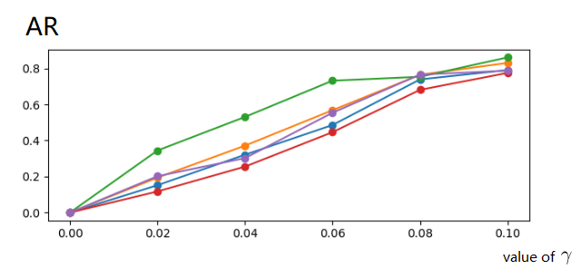
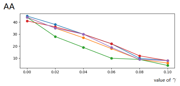
Figure 1: Left: Relation between $\gamma$ and the adversarial rate. Right: Relation between $\gamma$ and adversarial accuracy.

Attack	AC	AA in (5)		ARR in (6)
		$\widetilde{R}_{3}({\mathcal{F}},T)$	AR	$\widetilde{R}_{4}({\mathcal{F}},T)$	AR
No attack	83$\%$	49$\%$	0	0.0194	0
$L_{\infty,0.02}$	84$\%$	39$\%$	0.20	0.0151	0.22
$L_{\infty,0.04}$	85$\%$	27$\%$	0.45	0.0127	0.35
$L_{\infty,0.06}$	86$\%$	14$\%$	0.72	0.0092	0.53
$L_{\infty,0.08}$	87$\%$	6$\%$	0.87	0.0064	0.67
$L_{\infty,0.10}$	87$\%$	1$\%$	0.98	0.0044	0.77
$L_{0,10}$	80$\%$	26$\%$	0.45	0.0193	0
$L_{0,20}$	78$\%$	18$\%$	0.59	0.0187	0.03
$L_{0,30}$	72$\%$	9$\%$	0.71	0.0125	0.33

Table 5: Adversarial parameter attack for ${\mathcal{F}}_{R}$. AC: accuracy, AA: adversarial accuracy, AR: adversarial rate.

5.2.3 Affect of network depth and width on the adversarial parameter attack

We check how the network depth and width affect on the adversarial parameter attack. We use the $L_{\infty,\gamma}$ adversarial parameter attack for $\gamma=0.02,0.04$. Let ${\mathcal{F}}^{k}_{V}$ be the network which has the same width with ${\mathcal{F}}_{V}$ but has $k$ more layers, ${\mathcal{F}}_{V}(\alpha)$ the network which has the same depth with ${\mathcal{F}}_{V}$ but has $\alpha$ times width as ${\mathcal{F}}_{V}$. The results are given in Table 6. We can see that when the depth becomes larger, the attack becomes easier. This validates the results in section 4.2, for instance Corollary 4.5, where it shows that when the depth of the network becomes large, adversarial parameters exist.

The attack is much less sensitive to the width. The reason may be that there exist much redundancy on the width, similar to the results in [17, 25, 26], and the redundance can lead to limited search directions in the feature space and poor generalization performance, as shown in [21], so the attack is hard to improve when the width becomes larger.

Network	$\gamma=0$		$\gamma=0.02$			$\gamma=0.04$
	AC	AA	AC	AA	AR	AC	AA	AR
${\mathcal{F}}_{V}$	80$\%$	45$\%$	78$\%$	38$\%$	0.15	77$\%$	30$\%$	0.32
${\mathcal{F}}^{8}_{V}$	80$\%$	47$\%$	76$\%$	37$\%$	0.20	78$\%$	32$\%$	0.31
${\mathcal{F}}^{16}_{V}$	78$\%$	44$\%$	74$\%$	35$\%$	0.19	75$\%$	27$\%$	0.37
${\mathcal{F}}^{24}_{V}$	79$\%$	43$\%$	73$\%$	30$\%$	0.28	73$\%$	20$\%$	0.49
${\mathcal{F}}^{32}_{V}$	76$\%$	44$\%$	72$\%$	28$\%$	0.34	71$\%$	19$\%$	0.53
${\mathcal{F}}_{V}(1.25)$	80$\%$	42$\%$	77$\%$	37$\%$	0.12	76$\%$	29$\%$	0.29
${\mathcal{F}}_{V}(1.5)$	81$\%$	41$\%$	78$\%$	36$\%$	0.12	77$\%$	30$\%$	0.26
${\mathcal{F}}_{V}(2)$	78$\%$	44$\%$	76$\%$	39$\%$	0.11	74$\%$	31$\%$	0.28
${\mathcal{F}}_{V}(2.5)$	80$\%$	44$\%$	79$\%$	35$\%$	0.20	76$\%$	30$\%$	0.30

Table 6: Affect of width and depth on adversarial parameter attack for ${\mathcal{F}}_{V}$. AC: accuracy, AA: adversarial accuracy, AR: adversarial rate.

We can use $\widetilde{R}_{4}({\mathcal{F}},T)$ to measure the robustness and similar results are obtained, which are given in Table 7.

Network	$\gamma=0$	$\gamma=0.02$		$\gamma=0.04$
	$\widetilde{R}_{4}({\mathcal{F}},T)$	$\widetilde{R}_{4}({\mathcal{F}},T)$	AR	$\widetilde{R}_{4}({\mathcal{F}},T)$	AR
${\mathcal{F}}_{V}$	0.0770	0.0667	0.13	0.0481	0.36
${\mathcal{F}}^{8}_{V}$	0.0776	0.0686	0.11	0.0534	0.30
${\mathcal{F}}^{16}_{V}$	0.0815	0.0652	0.19	0.0479	0.40
${\mathcal{F}}^{24}_{V}$	0.0817	0.0630	0.21	0.0388	0.49
${\mathcal{F}}^{32}_{V}$	0.0808	0.0608	0.23	0.0392	0.48
${\mathcal{F}}_{V}(1.25)$	0.0750	0.0663	0.11	0.0524	0.29
${\mathcal{F}}_{V}(1.5)$	0.0763	0.0670	0.12	0.0563	0.25
${\mathcal{F}}_{V}(2)$	0.0750	0.0650	0.13	0.0499	0.32
${\mathcal{F}}_{V}(2.5)$	0.0775	0.0678	0.12	0.0489	0.35

Table 7: Affect of width and depth on adversarial parameter attack for ${\mathcal{F}}_{V}$. AR: adversarial rate

5.3 Direct adversarial parameters

We give experimental results for direct adversarial parameters introduced in section 2.2. We try to decrease the accuracies for samples with label 0 and keep the accuracies and robustness for other samples. The experimental results are for the network ${\mathcal{F}}_{V}$ and CIFAR-10 and are given in Table 8.

Attack	AC1	AA1	AC0	AR
$L_{\infty,0.02}$	77$\%$	35$\%$	11$\%$	0.65
$L_{\infty,0.04}$	78$\%$	40$\%$	3$\%$	0.83
$L_{\infty,0.06}$	79$\%$	42$\%$	1$\%$	0.92
$L_{\infty,0.08}$	80$\%$	43$\%$	1$\%$	0.95
$L_{\infty,0.1}$	80$\%$	45$\%$	1$\%$	0.99

Table 8: Direct adversarial parameter attack for ${\mathcal{F}}_{V}$. AC₁ and AA₁ are for samples with label $\neq 0$, AC₀ is the accuracy for samples with label $0$.

Comparing to Tables 8 and 4, we can see that direct adversarial parameters for a given label are much easier to compute than adversarial parameters. High quality direct adversarial parameters can be obtained by using perturbation ratios $6\%-10\%$. Results for network ${\mathcal{F}}_{R}$ are given in Table 9, from which we can see that it is slightly more difficult to attack ${\mathcal{F}}_{R}$.

Attack	AC1	AA1	AC0	AR
$L_{\infty,0.02}$	82$\%$	46$\%$	52$\%$	0.38
$L_{\infty,0.04}$	81$\%$	47$\%$	35$\%$	0.57
$L_{\infty,0.06}$	81$\%$	47$\%$	10$\%$	0.83
$L_{\infty,0.08}$	81$\%$	46$\%$	4$\%$	0.90
$L_{\infty,0.1}$	80$\%$	46$\%$	1$\%$	0.93

Table 9: Direc adversarial parameter attack for ${\mathcal{F}}_{R}$. AC₁ and AA₁ are for samples with label $\neq 0$, AC₀ is the accuracy for samples with label $0$.

5.4 Adversarial parameters for a given sample

We give experimental results for adversarial parameters for a given sample introduced in section 2.2. $\widetilde{R}_{2}({\mathcal{F}},x)=\min_{i\neq l_{x}}\{\frac{{\mathcal{F}}_{l_{x}}(x)-{\mathcal{F}}_{i}(x)}{||\nabla{\mathcal{F}}_{l_{x}}(x)-\nabla{\mathcal{F}}_{i}(x)||_{1}}\}$ is used to measure the robustness of ${\mathcal{F}}$ at sample $x$. Let $S$ be a subset of the test set containing 100 samples such that ${\mathcal{F}}$ gives the correct label for all of them and all samples in $S$ are robust in that, no adversarial samples were found using PGD-10 with $L_{\infty}=\frac{8}{255}$.

Attack	$\widetilde{R}_{2}({\mathcal{F}},x)$	$N_{1}$	$N_{2}$	AR
before attack	0.078	100	100	0
$L_{\infty,0.02}$	0.016	0	100	0.79
$L_{\infty,0.04}$	0.010	0	100	0.87
$L_{\infty,0.06}$	0.008	0	100	0.89
$L_{\infty,0.08}$	0.006	0	100	0.92
$L_{\infty,0.1}$	0.005	0	100	0.94

Table 10: Adversarial parameter attack to ${\mathcal{F}}_{V}$ for a given sample. AR: adversarial rate

For each sample $x\in S$, we compute $L_{\infty,\gamma}$ adversarial parameters and the average results are given in Table 10, where $N_{1}$ is the number of robust samples, and $N_{2}$ the number of samples which are given the correct labels. Comparing to Tables 8, 4, and 10, we can see that adversarial rates for a single sample are about the same as that for a given label. Similar results for network ${\mathcal{F}}_{R}$ are given in Table 11.

Attack	$\widetilde{R}_{2}({\mathcal{F}},x)$	$N_{1}$	$N_{2}$	AR
before attack	0.057	100	100	0
$L_{\infty,0.02}$	0.008	0	100	0.86
$L_{\infty,0.04}$	0.008	0	100	0.86
$L_{\infty,0.06}$	0.008	0	100	0.86
$L_{\infty,0.08}$	0.008	0	100	0.86
$L_{\infty,0.1}$	0.008	0	100	0.86

Table 11: Adversarial parameter attack to ${\mathcal{F}}_{R}$ for a given sample. AR: Adversarial Rate

6 Proofs for the theorems in section 4

6.1 Proofs of Theorems 4.1 and 4.2

We introduce several notations. Let $||x||_{-\infty}=\min_{i\in[n]}\{|x_{i}|\}$ for $x\in{\mathbb{R}}^{n}$, and $||W||_{-\infty,2}=\min_{i\in[a]}\{||W^{(i)}||_{2}\}$ for $W\in{\mathbb{R}}^{a\times b}$, where $W^{(i)}$ is the $i$-th row of $W$. If ${\mathcal{F}}$ is a network, we use ${\mathcal{F}}_{i}(x)$ to denote the $i$-th coordinate of ${\mathcal{F}}(x)$. A lemma is proved first.

Lemma 6.1.

Let $v\in{\mathbb{R}}^{n}$ and $v\neq 0$. Then there exists a vector $w\in{\mathbb{R}}^{n}$ such that $w\bot v$, $||w||_{\infty}=1$ and $||w||_{2}\geq\sqrt{n-1}$.

Proof.

Let $S=\arg\min_{S\subseteqq[n]}\{|\sum_{i\in S}|v_{i}|-\sum_{i\in[n]\setminus S}|v_{i}||\}$. We can assume $\sum_{i\in S}|v_{i}|-\sum_{i\in[n]\setminus S}|v_{i}|=k\geq 0$. For any $j\in S$ such that $v_{j}\neq 0$ and $S_{1}=S/\{j\}$, we have $|\sum_{i\in S_{1}}|v_{i}|-\sum_{i\in[n]/S_{1}}|v_{i}||=|2|v_{j}|-k|\geq k$, which means $k\leq|v_{j}|$.

We now define $w\in{\mathbb{R}}^{n}$. Set $w_{i}=1$ if $v_{i}=0$. Select a $j\in S$ such that $v_{j}\neq 0$ and let $w_{i}={\hbox{\rm{sign}}}(v_{i})$ if $i\in S/\{j\}$ and $v_{i}\neq 0$, and $w_{j}=\frac{-\sum_{i\in S}|v_{i}|+\sum_{i\in[n]\setminus S}|v_{i}|+|v_{j}|}{v_{j}}$. For $i\in[n]\setminus S$, let $w_{i}=-{\hbox{\rm{sign}}}(v_{i})$ if $v_{i}\neq 0$. It is easy to check that $||w||_{\infty}=1$, $||w||_{2}\geq\sqrt{n-1}$, and $w\bot v$. The lemma is proved. ∎

We now prove Theorem 4.1.

Proof.

By Lemma 6.1, there exists a vector $v\in{\mathbb{R}}^{n}$ such that $v\bot x_{0}$, $||v||_{2}\geq\sqrt{n-1}$ and $||v||_{\infty}=1$. Moreover, we can assume that at least $\eta n_{1}/2$ coordinates of ${\hbox{\rm{Relu}}}(W_{1}(x+\epsilon v)+b_{1})$ are bigger than $b$. If this is not valid, we just need to change $v$ to $-v$, and then ${\hbox{\rm{Relu}}}(W_{1}(x+\epsilon v)+b_{1})+{\hbox{\rm{Relu}}}(W_{1}(x-\epsilon v)+b_{1})\geq 2{\hbox{\rm{Relu}}}(W_{1}x+b_{1})$, since ${\hbox{\rm{Relu}}}(x)+{\hbox{\rm{Relu}}}(y)\geq{\hbox{\rm{Relu}}}(x+y)$ for all $x,y\in{\mathbb{R}}$. By condition $C_{3}$, at least $\eta n_{1}$ coordinates of $2{\hbox{\rm{Relu}}}(W_{1}x+b_{1})$ are bigger than $2b$, but fewer than $\eta n_{1}/2$ coordinates of ${\hbox{\rm{Relu}}}(W_{1}(x+\epsilon v)+b_{1})$ are bigger than $b$, so at least $\eta n_{1}/2$ coordinates of ${\hbox{\rm{Relu}}}(W_{1}(x-\epsilon v)+b_{1})$ are bigger than $b$.

Let $l_{2}\in[m]$ such that $l_{2}\neq l_{x_{0}}$, $\overline{W}_{2}=-(W_{2}^{(l_{x_{0}})}-W_{2}^{(l_{2})})\in{\mathbb{R}}^{1\times n_{1}}$, $U_{v}\in{\mathbb{R}}^{n_{1}\times n}$ all of whose rows are $\gamma v^{\tau}$ (the transposition of $v$), and $U={\hbox{\rm{diag}}}({\hbox{\rm{sign}}}(\overline{W}_{2}))\in{\mathbb{R}}^{n_{1}\times n_{1}}$. Let $\widetilde{W}_{1}=W_{1}+UU_{v}$ and

$$\widetilde{{\mathcal{F}}}(x)=W_{2}{\hbox{\rm{Relu}}}(\widetilde{W}_{1}x+b_{1})+b_{2}.$$

We will show that $\widetilde{{\mathcal{F}}}$ satisfies the condition of the theorem.

Since $v\bot x_{0}$, we have $\widetilde{{\mathcal{F}}}(x_{0})={\mathcal{F}}(x_{0})$ and $\widetilde{{\mathcal{F}}}$ gives the correct label for $x_{0}$. Since $||v||_{\infty}=1$, we have $||\widetilde{W}_{1}-W_{1}||_{\infty}=||UU_{v}||_{\infty}=||U_{v}||_{\infty}=||\gamma v||_{\infty}\leq\gamma$, and thus $\widetilde{{\mathcal{F}}}(x)\in H_{\gamma}(\Theta)$.

So it suffices to show that $\widetilde{{\mathcal{F}}}(x_{0}+\epsilon v)$ will not give $x_{0}+\epsilon v$ label $l_{x_{0}}$, which means that $\widetilde{{\mathcal{F}}}$ has adversarial samples to $x_{0}$ in $S_{\infty}(x_{0},\epsilon)$. Since

$$\begin{array}[]{ll}&\widetilde{{\mathcal{F}}}(x_{0}+\epsilon v)\\ =&W_{2}{\hbox{\rm{Relu}}}(\widetilde{W}_{1}(x_{0}+\epsilon v)+b_{1})+b_{2}\\ =&W_{2}{\hbox{\rm{Relu}}}(W_{1}(x_{0}+\epsilon v)+b_{1}+\epsilon UU_{v}v)+b_{2}\\ \end{array}$$

we have

$$\begin{array}[]{ll}&\widetilde{{\mathcal{F}}}_{l_{x_{0}}}(x_{0}+\epsilon v)-\widetilde{{\mathcal{F}}}_{l_{2}}(x_{0}+\epsilon v)\\ =&{\mathcal{F}}_{l_{x_{0}}}(x_{0}+\epsilon v)-{\mathcal{F}}_{l_{2}}(x_{0}+\epsilon v)+\\ &\overline{W}_{2}({\hbox{\rm{Relu}}}(W_{1}(x+\epsilon v)+b_{1})-{\hbox{\rm{Relu}}}(W_{1}(x+\epsilon v)+b_{1}+\epsilon UU_{v}v)).\\ \end{array}$$

Since $e({\hbox{\rm{Relu}}}(f)-{\hbox{\rm{Relu}}}(e+f))=-|f|(|{\hbox{\rm{Relu}}}(e)-{\hbox{\rm{Relu}}}(e+f))|$ for all $e,f\in{\mathbb{R}}$, we have

$$\begin{array}[]{ll}&-\overline{W}_{2}({\hbox{\rm{Relu}}}(W_{1}(x+\epsilon v)+b_{1})-{\hbox{\rm{Relu}}}(W_{1}(x+\epsilon v)+b_{1}+\epsilon UU_{v}v))\\ =&|\overline{W}_{2}|(|{\hbox{\rm{Relu}}}(W_{1}(x+\epsilon v)+b_{1})-{\hbox{\rm{Relu}}}(W_{1}(x+\epsilon v)+b_{1}+\epsilon UU_{v}v)|).\\ \end{array}$$

Since $\epsilon UU_{v}v=\epsilon\gamma||v||_{2}^{2}{\hbox{\rm{sign}}}(\overline{W}_{2})$ and $||v||_{2}\geq n-1$, each weight of $|\epsilon UU_{v}v|$ is at least $\epsilon\gamma(n-1)$. Note that if $e>0$ and $f\in{\mathbb{R}}$, then $|{\hbox{\rm{Relu}}}(e)-{\hbox{\rm{Relu}}}(e-f)|\geq\min\{e,|f|\}$. As a consequence, if $i$ satisfies $({\hbox{\rm{Relu}}}(W_{1}(x+\epsilon v)+b_{1}))_{i}>b$, then $(|{\hbox{\rm{Relu}}}(W_{1}(x+\epsilon v)+b_{1})-{\hbox{\rm{Relu}}}(W_{1}(x+\epsilon v)+b_{1}+\epsilon UU_{v}v)|)_{i}\geq\min\{\epsilon\gamma(n-1),b\}$. Since at least $\eta n_{1}/2$ coordinates of ${\hbox{\rm{Relu}}}(W_{1}(x+\epsilon v)+b_{1})$ are bigger than $b$, we have $||{\hbox{\rm{Relu}}}(W_{1}(x+\epsilon v)+b_{1})-{\hbox{\rm{Relu}}}(W_{1}(x+\epsilon v)+b_{1}+\epsilon UU_{v}v)||_{1}\geq\eta n_{1}/2\min\{\epsilon\gamma(n-1),b\}$. By condition $C_{2}$, it is easy see

$$\begin{array}[]{ll}&-\overline{W}_{2}({\hbox{\rm{Relu}}}(W_{1}(x+\epsilon v)+b_{1})-{\hbox{\rm{Relu}}}(W_{1}(x+\epsilon v)+b_{1}+\epsilon UU_{v}v))\\ =&|\overline{W}_{2}|(|{\hbox{\rm{Relu}}}(W_{1}(x+\epsilon v)+b_{1})-{\hbox{\rm{Relu}}}(W_{1}(x+\epsilon v)+b_{1}+\epsilon UU_{v}v)|)\\ \geq&||\overline{W}_{2}||_{-\infty}||{\hbox{\rm{Relu}}}(W_{1}(x+\epsilon v)+b_{1})-{\hbox{\rm{Relu}}}(W_{1}(x+\epsilon v)+b_{1}+\epsilon UU_{v}v)||_{1}\\ \geq&\min\{\epsilon\gamma(n-1),b\}cn_{1}\eta/2,\end{array}$$

that is, $\overline{W}_{2}({\hbox{\rm{Relu}}}(W_{1}(x+\epsilon v)+b_{1})-{\hbox{\rm{Relu}}}(W_{1}(x+\epsilon v)+b_{1}+\epsilon UU_{v}v))\leq-\min\{\epsilon\gamma(n-1),b\}cn_{1}\eta/2$. By condition $C_{1}$, we have ${\mathcal{F}}_{l_{x_{0}}}(x_{0}+\epsilon v)-{\mathcal{F}}_{l_{2}}(x_{0}+\epsilon v)\leq A$. Then we have

$$\begin{array}[]{ll}&\widetilde{{\mathcal{F}}}_{l_{x_{0}}}(x_{0}+\epsilon v)-\widetilde{{\mathcal{F}}}_{l_{2}}(x_{0}+\epsilon v)\\ =&{\mathcal{F}}_{l_{x_{0}}}(x_{0}+\epsilon v)-{\mathcal{F}}_{l_{2}}(x_{0}+\epsilon v)+\\ &\overline{W}_{2}({\hbox{\rm{Relu}}}(W_{1}(x+\epsilon v)+b_{1})-{\hbox{\rm{Relu}}}(W_{1}(x+\epsilon v)+b_{1}+\epsilon UU_{v}v))\\ \leq&A-\min\{\epsilon\gamma(n-1),b\}cn_{1}\eta/2<0.\end{array}$$

Thus if $n_{1}>\frac{2A}{\min\{\epsilon\gamma(n-1),b\}c\eta}$, then $\widetilde{{\mathcal{F}}}_{l_{x_{0}}}(x_{0}+\epsilon v)-\widetilde{{\mathcal{F}}}_{l_{2}}(x_{0}+\epsilon v)<0$ and the label of $\widetilde{{\mathcal{F}}}(x_{0}+\epsilon v)$ is not $l_{x_{0}}$. The theorem is proved. ∎

We now prove Theorem 4.2.

Proof.

By condition $C_{4}$, for $l\in[m]$, there exist $v_{l}\in{\mathbb{R}}^{n}$ such that $v_{l}\bot S$, $v_{l}\bot v_{k}$ for $l\neq k$, $||v_{l}||_{2}=1$. Then $||v_{l}||_{\infty}\leq 1$.

By condition $C_{3}$, at least $\eta n_{1}/2$ coordinates of ${\hbox{\rm{Relu}}}(W_{1}(x+\epsilon v_{l_{x}})+b_{1})$ are bigger than $b$ or at least $\eta n_{1}/2$ coordinates of ${\hbox{\rm{Relu}}}(W_{1}(x-\epsilon v_{l_{x}})+b_{1})$ are bigger than $b$, similar to the proof of Theorem 4.1.

For convenience, we write $G(x,y):({\mathbb{R}}^{n},{\mathbb{R}})\to{\mathbb{R}}$ as $G(x,y)=||{\hbox{\rm{sign}}}(x-yI_{n})||_{0}$, where $I_{n}$ is the vector with entries 1. It is easy to see that, $G(x,b)$ is the number of coordinates of $x$ that are bigger than $b$. So we have $G({\hbox{\rm{Relu}}}(W_{1}(x+\epsilon v_{l_{x}})+b_{1}),b)\geq\eta n_{1}/2$ or $G({\hbox{\rm{Relu}}}(W_{1}(x-\epsilon v_{l_{x}})+b_{1}),b)\geq\eta n_{1}/2$ for all $x$, and hence for $l\in[m]$, we have

$$P_{x\sim D_{x}}(G({\hbox{\rm{Relu}}}(W_{1}(x+\epsilon v_{l_{x}})+b_{1}),b)\geq\eta n_{1}/2\hbox{ or }G({\hbox{\rm{Relu}}}(W_{1}(x-\epsilon v_{l_{x}})+b_{1}),b)\geq\eta n_{1}/2\,|\,l_{x}=l)=1.$$

For events $e$ and $f$, $P(e\ \hbox{or}\ f)\leq P(e)+P(f)$. We thus have $P_{x\sim D_{x}}(G({\hbox{\rm{Relu}}}(W_{1}(x+\epsilon v_{l_{x}})+b_{1}),b)\geq\eta n_{1}/2\,|\,l_{x}=l)\geq 0.5$ or $P_{x\sim D_{x}}(G({\hbox{\rm{Relu}}}(W_{1}(x-\epsilon v_{l_{x}})+b_{1}),b)\geq\eta n_{1}/2\,|\,l_{x}=l)\geq 0.5$. Without loss of generality, we can assume that for any $l\in[m]$, $P_{x\sim D_{x}}(G({\hbox{\rm{Relu}}}(W_{1}(x+\epsilon v_{l_{x}})+b_{1}),b)\geq\eta n_{1}/2\,|\,l_{x}=l)\geq 0.5$. Therefore,

$$\begin{array}[]{ll}&P_{x\sim D_{x}}(G({\hbox{\rm{Relu}}}(W_{1}(x+\epsilon v_{l_{x}})+b_{1}),b)\geq\eta n_{1}/2)\\ =&\sum_{l\in[m]}P_{x\sim D_{x}}(l_{x}=l)P_{x\sim D_{x}}(G({\hbox{\rm{Relu}}}(W_{1}(x+\epsilon v_{l_{x}})+b_{1}),b)\geq\eta n_{1}/2\,|\,l_{x}=l)\\ \geq&0.5\sum_{l\in[m]}P_{x\sim D_{x}}(l_{x}=l)\\ =&0.5.\end{array}$$

For $l\in[m]$, let $\overline{W}_{2}^{(l)}=W_{2}^{(l)}-W_{2}^{(l+1)}$, where $W_{2}^{(m+1)}=W_{2}^{(1)}$. Now assume $U^{l}_{v}\in{\mathbb{R}}^{n_{1}\times n}$, whose rows are all $\gamma v_{l}$, and $U_{l}={\hbox{\rm{diag}}}({\hbox{\rm{sign}}}(\overline{W}_{2}^{(l)}))$. Let $\widetilde{W}_{1}=W_{1}+\frac{1}{m}\sum_{l=1}^{m}U_{l}U^{l}_{v}$, and

$$\widetilde{{\mathcal{F}}}(x)=W_{2}{\hbox{\rm{Relu}}}(\widetilde{W}_{1}x+b_{1})+b_{2}.$$

We will show that $\widetilde{{\mathcal{F}}}(x)$ satisfies the conditions of the theorem.

It is easy to see that $\widetilde{{\mathcal{F}}}$ is in ${\mathcal{H}}_{\gamma}(\Theta)$. For any $x\in S$, $\widetilde{W}_{1}x=W_{1}x+\frac{1}{m}\sum_{l=1}^{m}(U_{l}U^{l}_{v})x=W_{1}x$, which means $\widetilde{{\mathcal{F}}}(x)={\mathcal{F}}(x)$ and the accuracy of $\widetilde{{\mathcal{F}}}$ over $D_{x}$ is equal to that of ${\mathcal{F}}$.

Let $x\in S$ satisfy $G({\hbox{\rm{Relu}}}(W_{1}(x+\epsilon v_{l_{x}})+b_{1}),b)>\eta n_{1}/2$ and $l_{2}\neq l_{x}$. By conditions $C_{1}$ and $C_{2}$ and similar to the proof of Theorem 4.1, we have

$$\begin{array}[]{ll}&\widetilde{{\mathcal{F}}}_{l_{x}}(x+\epsilon v_{l_{x}})-\widetilde{{\mathcal{F}}}_{l_{2}}(x+\epsilon v_{l_{x}})\\ =&{\mathcal{F}}_{l_{x}}(x+\epsilon v_{l_{x}})-{\mathcal{F}}_{l_{2}}(x+\epsilon v_{l_{x}})+\\ &W^{(l_{x})}_{c}({\hbox{\rm{Relu}}}(W_{1}(x+\epsilon v_{l_{x}})+b_{1})-{\hbox{\rm{Relu}}}(W_{1}(x+\epsilon v_{l_{x}})+b_{1}+\epsilon U_{l}U^{l}_{v}v/m))\\ \leq&A-\min\{\epsilon\gamma/m,b\}cn_{1}\eta/2<0.\end{array}$$

Thus $\widetilde{{\mathcal{F}}}$ does not give label $l_{x}$ to $x+\epsilon v_{l_{x}}$ and $\widetilde{{\mathcal{F}}}$ has an adversarial sample of $x$ in $S_{\infty}(x,\epsilon)$. Furthermore, since $P_{x\sim D_{x}}(G({\hbox{\rm{Relu}}}(W_{1}(x+\epsilon v_{l_{x}})+b_{1}),b)\geq\gamma n_{1}/2)>0.5$, we have

$$P_{x\sim D_{x}}(\widetilde{{\mathcal{F}}}\ has\ an\ adversarial\ sample\ of\ x\ in\ S_{\infty}(x_{,}\epsilon))>0.5.$$

The theorem is proved. ∎

6.2 Proofs of Theorems 4.3 and 4.4

We first prove two lemmas.

Lemma 6.2.

For $l\in[m]$, let $S_{l}$ be a non-empty bounded closed subset of ${\mathbb{R}}^{n\times n}$ such that $W\in S_{l}$ implies $-W\in S_{l}$. Also let $S_{0}$ be a non-empty bounded closed subset of ${\mathbb{R}}^{1\times n}$ such that $x\in S_{0}$ implies $-x\in S_{0}$. Let $U_{0}\in{\mathbb{R}}^{1\times n}$ and $U_{l}\in{\mathbb{R}}^{n\times n}$ for $l\in[m]$. Define maps: $T_{0}(x):{\mathbb{R}}^{1\times n}\to{\mathbb{R}}^{1\times n}$ by $T_{0}(x)=x\prod_{l=1}^{m}U_{l}$, and for $l\in[m]$, $T_{l}(W):{\mathbb{R}}^{n\times n}\to{\mathbb{R}}^{1\times n}$ by $T_{l}(W)=U_{0}(\prod_{j=1}^{l-1}U_{j})W(\prod_{j=l+1}^{m}U_{j})$. Then

$$\max_{x_{l}\in S_{l},\forall 0\leq l\leq m}\{||\prod_{l=0}^{m}(x_{l}+U_{l})||_{2}^{2}\}\geq||\prod_{l=0}^{m}U_{l}||^{2}_{2}+\sum_{l=0}^{m}\max_{x_{l}\in S_{l}}\{||T_{l}(x_{l})||_{2}^{2}\}$$

Proof.

For $l\in[m]$, let $u_{l}=\arg\max_{x\in S_{l}}||T_{l}(x)||_{2}^{2}$, which exists because $S_{l}$ is bounded and closed. Then

$$\begin{array}[]{ll}&\max_{x_{l}\in S_{l},\forall 0\leq l\leq m}\{||\prod_{l=0}^{m}(x_{l}+U_{l})||_{2}^{2}\}\\ \geq&\max_{x_{l}\in\{u_{l},-u_{l}\},\forall 0\leq l\leq m}\{||\prod_{l=0}^{m}(x_{l}+U_{l})||_{2}^{2}\}\\ =&\frac{1}{2^{m+1}}\sum_{x_{l}\in\{u_{l},-u_{l}\},\forall 0\leq l\leq m}||\prod_{l=0}^{m}(x_{l}+U_{l})||_{2}^{2}\\ =&\sum_{M_{l}\in\{u_{l},U_{l}\},\forall 0\leq l\leq m}||\prod_{l=0}^{m}M_{l}||_{2}^{2}\\ \geq&||\prod_{l=0}^{m}U_{l}||_{2}+\sum_{l=0}^{m}||T_{l}(u_{l})||_{2}^{2}\\ =&||\prod_{l=0}^{m}U_{l}||_{2}+\sum_{l=0}^{m}\max_{x_{l}\in S_{l}}\{||T_{l}(x_{l})||_{2}^{2}\}\end{array}$$

The lemma is proved. ∎

Lemma 6.3.

For $l\in[m]$, let $S_{l}$ be a non-empty closed subset of bounded functions from ${\mathbb{I}}^{k}$ to $R^{n\times n}$ such that $c(x)\in S_{l}$ implies $-c(x)\in S_{l}$. Also let $S_{0}$ be a non-empty closed subset of bounded functions from ${\mathbb{I}}^{k}$ to ${\mathbb{R}}^{1\times n}$ such that $c(x)\in S_{0}$ implies $-c(x)\in S_{0}$. Assume $U_{0}(x):{\mathbb{I}}^{k}\to{\mathbb{R}}^{1\times n}$, $U_{l}(x):{\mathbb{I}}^{k}\to{\mathbb{R}}^{n\times n}$ for $l\in[m]$. Define maps: $T_{0}(c,x):(S_{0},{\mathbb{I}}^{k})\to{\mathbb{R}}^{1\times n}$ by $T_{0}(c,x)=c(x)\prod_{l=1}^{m}U_{l}(x)$; and $T_{l}(c,x):(S_{l},{\mathbb{I}}^{k})\to{\mathbb{R}}^{1\times n}$ by $T_{l}(x)=(\prod_{j=0}^{l-1}U_{j}(x))c(x)(\prod_{j=l+1}^{m}U_{j}(x))$ for $l\in[m]$. Then we have

$$\max_{c_{l}(x)\in S_{l},\forall 0\leq l\leq m}\displaystyle\{\int_{x\sim D_{x}}||\prod_{l=0}^{m}(c_{l}(x)+U_{l}(x))||_{2}^{2}\displaystyle\}\geq\int_{x\sim D_{x}}||\prod_{l=0}^{m}U_{l}(x)||^{2}_{2}+\sum_{l=0}^{m}\max_{c_{l}(x)\in S_{l}}\{\int_{x\sim{D_{x}}}||T_{l}(c_{l},x)||_{2}^{2}\}.$$

Proof.

Denote $\overline{c_{l}}(x)=\arg\max_{c\in S_{l}}||\int_{x\sim D_{x}}T_{l}(c,x)||_{2}^{2}$, which must exist because $S_{l}$ is closed and its elements are bounded. Then

$$\begin{array}[]{ll}&\max_{c_{l}(x)\in S_{l},\forall 0\leq l\leq m}\{\int_{x\sim D_{x}}||\prod_{l=0}^{m}(c_{l}(x)+U_{l}(x))||_{2}^{2}\}\\ \geq&\max_{c_{l}(x)\in\{\overline{c_{l}}(x),-\overline{c_{l}}(x)\},\forall 0\leq l\leq m}\{\int_{x\sim D_{x}}||\prod_{l=0}^{m}(c_{l}(x)+U_{l}(x))||_{2}^{2}\}\\ \geq&\frac{1}{2^{m+1}}\sum_{c_{l}\in\{\overline{c_{l}}(x),-\overline{c_{l}}(x)\},\forall 0\leq l\leq m}\int_{x\sim D_{x}}||\prod_{l=0}^{m}(c_{l}(x)+U_{l}(x))||_{2}^{2}\\ =&\sum_{M_{l}(x)\in\{\overline{c_{l}}(x),U_{l}(x)\},\forall 0\leq l\leq m}||\int_{x\sim D_{x}}\prod_{l=0}^{m}M_{l}(x)||_{2}^{2}\\ \geq&\int_{x\sim D_{x}}||\prod_{l=0}^{m}U_{l}(x)||^{2}_{2}+\sum_{l=0}^{m}\int_{x\sim D_{x}}||T_{l}(\overline{c_{l}},x)||_{2}^{2}\\ =&\int_{x\sim D_{x}}||\prod_{l=0}^{m}U_{l}||_{2}+\sum_{l=0}^{m}\max_{c_{l}\in S_{l}}\{\int_{x\sim D_{x}}||T_{l}(c_{l},x)||_{2}^{2}\}.\end{array}$$

The lemma is proved. ∎

We now prove Theorem 4.3.

Proof.

Let $S_{l}$ be the set of $Q\in{\mathbb{R}}^{n\times n}$ satisfying $||Q||_{\infty}\leq\gamma$ and $Q{\mathcal{F}}^{l-1}(x_{0})=0$ for $l\in[L+1]$. Note that $Q$ satisfies $n(l+1)$ linear equations and has $n^{2}$ variables. Since $n\gg l$ in DNNs, we can assume that $S_{l}$ is not empty. Let ${\mathbb{F}}$ be the set of networks $\widetilde{{\mathcal{F}}}:{\mathbb{R}}^{n}\to{\mathbb{R}}^{m}$ satisfying

$$\widetilde{{\mathcal{F}}}(x)=\widetilde{W}_{L+1}\sigma(\widetilde{W}_{L}\sigma(\widetilde{W}_{L-1}\sigma(\dots\sigma(\widetilde{W}_{1}x))))$$

where $\widetilde{W}_{l}-W_{l}\in S_{l}$ for all $l\in[L+1]$. We have $\widetilde{{\mathcal{F}}}^{l}(x_{0})={\mathcal{F}}^{l}(x_{0})$ for $l\in[L+1]$. So $\widetilde{{\mathcal{F}}}(x_{0})=l_{x_{0}}$ if $\widetilde{{\mathcal{F}}}\in{\mathbb{F}}$. It is also easy to see that ${\mathbb{F}}\subset{\mathcal{H}}_{\gamma}(\Theta)$. So it suffices to prove

$$\min_{\widetilde{{\mathcal{F}}}\in{\mathbb{F}}}\{\frac{R(\widetilde{{\mathcal{F}}},x_{0})}{R({\mathcal{F}},x_{0})}\}\leq 1-\frac{\gamma^{2}((L-1)(\sin(r)cb)^{2}+c^{2}+(2\sin(r)b)^{2})}{4A+\gamma^{2}((L-1)(\sin(r)cb)^{2}+c^{2}+(2\sin(r)b)^{2})}.$$

Let $l_{2}=\arg\min_{i\neq l_{x_{0}}}\{\frac{|{\mathcal{F}}_{l_{x_{0}}}(x_{0})-{\mathcal{F}}_{i}(x_{0})|^{2}}{||\nabla({\mathcal{F}}_{l_{x_{0}}}(x_{0}))-\nabla({\mathcal{F}}_{i}(x_{0}))||_{2}^{2}}I({\mathcal{F}}_{l_{x_{0}}}(x_{0})>{\mathcal{F}}_{i}(x_{0}))\}$. Then

$$R({\mathcal{F}},x_{0})=\frac{|{\mathcal{F}}_{l_{x_{0}}}(x_{0})-{\mathcal{F}}_{l_{2}}(x_{0})|^{2}}{||\nabla({\mathcal{F}}_{l_{x_{0}}}(x_{0}))-\nabla({\mathcal{F}}_{l_{2}}(x_{0}))||_{2}^{2}}.$$

Then for all $\widetilde{{\mathcal{F}}}\in{\mathbb{F}}$, we have

$$R(\widetilde{{\mathcal{F}}},x_{0})\leq\frac{|\widetilde{{\mathcal{F}}}_{l_{x}}(x_{0})-\widetilde{{\mathcal{F}}}_{l_{2}}(x_{0})|^{2}}{||\nabla(\widetilde{{\mathcal{F}}}_{l_{x}}(x_{0}))-\nabla(\widetilde{{\mathcal{F}}}_{l_{2}}(x_{0}))||_{2}^{2}}=\frac{|{\mathcal{F}}_{l_{x}}(x_{0})-{\mathcal{F}}_{l_{2}}(x_{0})|^{2}}{||\nabla(\widetilde{{\mathcal{F}}}_{l_{x}}(x_{0}))-\nabla(\widetilde{{\mathcal{F}}}_{l_{2}}(x_{0}))||_{2}^{2}}$$

So we have

$$\begin{array}[]{ll}&\min_{\widetilde{{\mathcal{F}}}\in{\mathbb{F}}}\{\frac{R(\widetilde{{\mathcal{F}}},x_{0})}{R({\mathcal{F}},x_{0})}\}\\ \leq&\min_{\widetilde{{\mathcal{F}}}\in{\mathbb{F}}}\{\frac{|{\mathcal{F}}_{l_{x}}(x_{0})-{\mathcal{F}}_{l_{2}}(x_{0})|^{2}}{||\nabla(\widetilde{{\mathcal{F}}}_{l_{x}}(x_{0}))-\nabla(\widetilde{{\mathcal{F}}}_{l_{2}}(x_{0}))||_{2}^{2}}/\frac{|{\mathcal{F}}_{l_{x}}(x)-{\mathcal{F}}_{l_{2}}(x)|^{2}}{||\nabla({\mathcal{F}}_{l_{x}}(x))-\nabla({\mathcal{F}}_{l_{2}}(x))||_{2}^{2}}\}\\ \leq&\min_{\widetilde{{\mathcal{F}}}\in{\mathbb{F}}}\{\frac{||\nabla({\mathcal{F}}_{l_{x}}(x_{0}))-\nabla({\mathcal{F}}_{l_{2}}(x_{0}))||_{2}^{2}}{||\nabla(\widetilde{{\mathcal{F}}}_{l_{x}}(x_{0}))-\nabla(\widetilde{{\mathcal{F}}}_{l_{2}}(x_{0}))||_{2}^{2}}\}.\end{array}$$ (19)

To prove the theorem, we will first find a lower bound for $\max_{\widetilde{{\mathcal{F}}}\in{\mathbb{F}}}\{||\nabla(\widetilde{{\mathcal{F}}}_{l_{x}}(x_{0}))-\nabla(\widetilde{{\mathcal{F}}}_{l_{2}}(x_{0}))||_{2}\}$. Let $J_{l}(x)={\hbox{\rm{diag}}}({\hbox{\rm{sign}}}({\mathcal{F}}^{l}(x))):\ {\mathbb{R}}^{n}\to{\mathbb{R}}^{n\times n}$ for $l\in[L]$. Then

$$\frac{\nabla{\mathcal{F}}_{i}(x)}{\nabla x}=W^{i}_{L+1}(J_{L}(x)W_{L})(J_{L-1}(x)W_{L-1})\dots(J_{1}(x)W_{1}).$$

Let $A_{l}(x)=\frac{\nabla{\mathcal{F}}^{L}(t)}{\nabla{\mathcal{F}}^{l}(t)}|_{t=x}$ and $B_{l}(x)=\frac{\nabla{\mathcal{F}}^{l}(t)}{\nabla t}|_{t=x}$ for $l\in[L]$. Then we have

$$\begin{array}[]{ll}A_{l}(x)=(J_{L}(x)W_{L})(J_{L-1}(x)W_{L-1})\dots(J_{l+1}(x)W_{l+1})\\ B_{l}(x)=(J_{l}(x)W_{l})(J_{l-1}(x)W_{l-1})\dots(J_{1}(x)W_{1}).\end{array}$$

Let $A_{l}=A_{l}(x_{0})$, $B_{l}=B_{l}(x_{0})$, $J_{l}=J_{l}(x_{0})$. Then for all $\widetilde{{\mathcal{F}}}\in{\mathbb{F}}$,

$$\frac{\nabla\widetilde{{\mathcal{F}}}_{i}(x)}{\nabla x}|_{x=x_{0}}=\widetilde{W}_{L+1}^{i}(J_{L}\widetilde{W}_{L})(J_{L-1}\widetilde{W}_{L-1})\dots(J_{1}\widetilde{W}_{1}).$$

Denote $\overline{W}_{l}=\widetilde{W}_{l}-W_{l}\in S_{l}$ for $l\in[L+1]$. We have

$$\begin{array}[]{ll}&\nabla(\widetilde{{\mathcal{F}}}_{l_{x}}(x_{0}))-\nabla(\widetilde{{\mathcal{F}}}_{l_{2}}(x_{0}))\\ =&(\widetilde{W}_{L+1}^{(l_{x})}-\widetilde{W}_{L+1}^{(l_{2})})(J_{L}\widetilde{W}_{L})(J_{L-1}\widetilde{W}_{L-1})\dots(J_{1}\widetilde{W}_{1})\\ =&(W_{L+1}^{(l_{x})}-W_{L+1}^{(l_{2})}+\overline{W}_{L+1}^{(l_{x})}-\overline{W}_{L+1}^{(l_{2})})(J_{L}(W_{L}+\overline{W}_{L}))(J_{L-1}(W_{L-1}+\overline{W}_{L-1}))\dots(J_{1}(W_{1}+\overline{W}_{1})).\\ \end{array}$$

Now, let $\gamma(\overline{W}_{1})=(W_{L+1}^{(l_{x})}-W_{L+1}^{(l_{2})})A_{1}J_{1}\overline{W}_{1}$, $M_{i}(\overline{W}_{i})=(W_{L+1}^{(l_{x})}-W_{L+1}^{(l_{2})})A_{i}J_{i}\overline{W}_{i}B_{i-1}$, where $i\in\{2,3,\dots,L\}$, $M_{L+1}(\overline{W}_{L+1})=(\overline{W}_{L+1}^{(l_{x})}-\overline{W}_{L+1}^{(l_{2})})B_{L}$. By Lemma 6.2, we have

$$\begin{array}[]{ll}&\max_{\widetilde{{\mathcal{F}}}\in{\mathbb{F}}}\{||\nabla(\widetilde{{\mathcal{F}}}_{l_{x}}(x_{0}))-\nabla(\widetilde{{\mathcal{F}}}_{l_{2}}(x_{0}))||^{2}_{2}\}\\ \geq&\max_{\overline{W}_{j}\in S_{j},j\in[L+1]}\{||\nabla({\mathcal{F}}_{l_{x}}(x_{0}))-\nabla({\mathcal{F}}_{l_{2}}(x_{0}))||_{2}^{2}+\sum_{i=1}^{L+1}||M_{i}(\overline{W}_{i})||^{2}_{2}\}\\ =&||\nabla({\mathcal{F}}_{l_{x}}(x_{0}))-\nabla({\mathcal{F}}_{l_{2}}(x_{0}))||_{2}^{2}+\sum_{i=1}^{L+1}\max_{\overline{W}_{i}\in S_{i}}\{||M_{i}(\overline{W}_{i})||^{2}_{2}\}.\end{array}$$

It is easy to see for any $l\in[L]$, $(W_{L+1}^{(l_{x})}-W_{L+1}^{(l_{2})})A_{l}=\frac{\nabla{\mathcal{F}}_{l_{x}}(t)-{\mathcal{F}}_{l_{2}}(t)}{\nabla{\mathcal{F}}^{l}(t)}|_{t=x_{0}}$, so by condition $C_{3}$, we have $||(W_{L+1}^{(l_{x})}-W_{L+1}^{(l_{2})})A_{i}||_{-\infty}>c$. Let $S^{1}_{l}$ be the subset of $S_{l}$ containing those $C$ which have at most one nonzero row. Hence, for $x\in{\mathbb{R}}^{1\times n}$ and $M\in{\mathbb{R}}^{n\times n}$, if at most one row of $M$ is nonzero, we have $||xM||_{\infty}=\max_{i,j\in[n]}\{|x_{i}M_{i,j}|\}\geq||x||_{-\infty}||M||_{\infty}$, where $x_{i}$ is the $i$-th weight of $x$, $M_{i,j}$ is the weight of $M$ at $i$-th row and $j$-th column. Thus

$$\begin{array}[]{ll}&\max_{\overline{W}_{1}\in S_{1}}\{||\gamma(\overline{W}_{1})||_{2}\}\\ =&\max_{\overline{W}_{1}\in S_{1}}\{||(W_{L+1}^{(l_{x})}-W_{L+1}^{(l_{2})})A_{1}J_{1}\overline{W}_{1}||_{2}\}\\ \geq&\max_{\overline{W}_{1}\in S_{1}}\{||(W_{L+1}^{(l_{x})}-W_{L+1}^{(l_{2})})A_{1}J_{1}\overline{W}_{1}||_{\infty}\}\\ \geq&\max_{\overline{W}_{1}\in S^{1}_{1}}\{||(W_{L+1}^{(l_{x})}-W_{L+1}^{(l_{2})})A_{1}J_{1}\overline{W}_{1}||_{\infty}\}\\ \geq&||(W_{L+1}^{(l_{x})}-W_{L+1}^{(l_{2})})A_{1}||_{-\infty}\max_{\overline{W}_{1}\in S^{1}_{1}}\{||J_{1}\overline{W}_{1}||_{\infty}\}\\ \geq&\gamma c.\end{array}$$

Moreover, by condition $C_{4}$, there exists a column $L_{i-1}$ of $B_{i-1}$ such that $\pi-r\geq\alpha({\mathcal{F}}^{i-1}(x_{0}),L_{i-1})\geq r$, where $\alpha(x,y)$ is the angle between $x,y$. Therefore, there exists a vector $v_{i}\in{\mathbb{R}}^{n}$ such that $v\bot{\mathcal{F}}^{i-1}(x)$, $||v_{i}||_{\infty}=\gamma$ and consider condition $C_{2}$, we have $\langle v_{i},L_{i-1}\rangle=||v_{i}||_{2}||L_{i-1}||_{2}\cos(\pi/2-r)\geq\sin(r)b\gamma$.

Then $\max_{\overline{W}_{i}\in S^{1}_{i}}||J_{i}\overline{W}_{i}B_{i-1}||_{\infty}\geq\sin(r)b\gamma$, because there must exist a $\overline{W}_{i}\in S^{1}_{i}$ whose only nonzero row is $v_{i}$ and $J_{i}\overline{W}_{i}=\overline{W}_{i}$. For $l\in\{2,3,\dots,L\}$, by condition $C_{3}$, we have

$$\begin{array}[]{ll}&\max_{\overline{W}_{l}\in S_{l}}\{||M_{l}(\overline{W}_{l})||_{2}\\ =&\max_{\overline{W}_{l}\in S_{l}}\{||(W_{L+1}^{(l_{x})}-W_{L+1}^{(l_{2})})A_{i}J_{l}\overline{W}_{l}B_{l-1}||_{2}\}\\ \geq&\max_{\overline{W}_{l}\in S_{l}}\{||(W_{L+1}^{(l_{x})}-W_{L+1}^{(l_{2})})A_{l}J_{l}\overline{W}_{l}B_{l-1}||_{\infty}\}\\ \geq&\max_{\overline{W}_{l}\in S^{1}_{l}}\{||(W_{L+1}^{(l_{x})}-W_{L+1}^{(l_{2})})A_{l}J_{l}\overline{W}_{l}B_{l-1}||_{\infty}\}\\ \geq&||(W_{L+1}^{(l_{x})}-W_{L+1}^{(l_{2})})A_{1}||_{-\infty}\max_{\overline{W}_{l}\in S_{l}}||J_{l}\overline{W}_{l}B_{l-1}||_{\infty}\\ \geq&\gamma\sin(r)cb.\end{array}$$

Similarly,

$$\begin{array}[]{ll}&\max_{\overline{W}_{L+1}\in S_{L+1}}\{||M_{L+1}(\overline{W}_{L+1})||_{2}\}\\ =&\max_{\overline{W}_{L+1}\in S_{L+1}}\{||(\overline{W}_{L+1}^{(l_{x})}-\overline{W}_{L+1}^{(l_{2})})B_{L}||_{2}\}\\ \geq&\max_{\overline{W}_{L+1}\in S_{L+1}}\{||(\overline{W}_{L+1}^{(l_{x})}-\overline{W}_{L+1}^{(l_{2})})B_{L}||_{\infty}\}\\ \geq&2\sin(r)b\gamma.\\ \end{array}$$

Then we obtain the desired lower bound:

$$\begin{array}[]{ll}&\max_{\widetilde{{\mathcal{F}}}\in{\mathbb{F}}}\{||\nabla(\widetilde{{\mathcal{F}}}_{l_{x}}(x_{0}))-\nabla(\widetilde{{\mathcal{F}}}_{l_{2}}(x_{0}))||^{2}_{2}\}\\ \geq&\max_{\overline{W}_{j}\in S_{j},j\in[L+1]}\{||\nabla({\mathcal{F}}_{l_{x}}(x_{0}))-\nabla({\mathcal{F}}_{l_{2}}(x_{0}))||_{2}^{2}+\sum_{l=1}^{L+1}||M_{l}(\overline{W}_{l})||^{2}_{2}\}\\ \geq&||\nabla({\mathcal{F}}_{l_{x}}(x))-\nabla({\mathcal{F}}_{l_{2}}(x))||_{2}^{2}+\gamma^{2}((L-1)(\sin(r)cb)^{2}+c^{2}+(2\sin(r)b)^{2}).\end{array}$$

By condition $C_{1}$ and the lower bound just obtained, we have

$$\begin{array}[]{ll}&\min_{\widetilde{{\mathcal{F}}}\in{\mathbb{F}}}\{\frac{||\nabla({\mathcal{F}}_{l_{x}}(x_{0}))-\nabla({\mathcal{F}}_{l_{2}}(x_{0}))||_{2}^{2}}{||\nabla(\widetilde{{\mathcal{F}}}_{l_{x}}(x_{0}))-\nabla(\widetilde{{\mathcal{F}}}_{l_{2}}(x_{0}))||_{2}^{2}}\}\\ \leq&\frac{||\nabla({\mathcal{F}}_{l_{x}}(x_{0}))-\nabla({\mathcal{F}}_{l_{2}}(x_{0}))||_{2}^{2}}{||\nabla({\mathcal{F}}_{l_{x}}(x_{0}))-\nabla({\mathcal{F}}_{l_{2}}(x_{0}))||_{2}^{2}+\gamma^{2}((L-1)(\sin(r)cb)^{2}+c^{2}+(2\sin(r)b)^{2})}\\ =&1-\frac{\gamma^{2}((L-1)(\sin(r)cb)^{2}+c^{2}+(2\sin(r)b)^{2})}{||\nabla({\mathcal{F}}_{l_{x}}(x_{0}))-\nabla({\mathcal{F}}_{l_{2}}(x_{0}))||_{2}^{2}+\gamma^{2}((L-1)(\sin(r)cb)^{2}+c^{2}+(2\sin(r)b)^{2})}\\ \leq&1-\frac{\gamma^{2}((L-1)(\sin(r)cb)^{2}+c^{2}+(2\sin(r)b)^{2})}{4A+\gamma^{2}((L-1)(\sin(r)cb)^{2}+c^{2}+(2\sin(r)b)^{2})}.\end{array}$$

The theorem is proved. ∎

We now prove Theorem 4.4.

Proof.

The proof is similar to that of Theorem 4.3, so certain details are omitted. Let $T_{l}=\{{\mathcal{F}}^{l-1}(x)\,|\,x\in S\}\subset{\mathbb{R}}$, and $S_{l}$ the set of $Q\in{\mathbb{R}}^{n\times n}$ such that $||Q||_{\infty}\leq\gamma$ and $Qt=0$ for all $t\in T_{l}$ and $l\in[L+1]$. $S_{l}$ must contain non-zero elements because of condition $C_{4}$.

Let ${\mathbb{F}}$ be the set of networks $\widetilde{{\mathcal{F}}}\in{\mathbb{R}}^{n}\to{\mathbb{R}}^{m}$

$$\widetilde{{\mathcal{F}}}(x)=\widetilde{W}_{L+1}\sigma(\widetilde{W}_{L}\sigma(\widetilde{W}_{L-1}\sigma(\dots\sigma(\widetilde{W}_{1}x))))$$

where $\widetilde{W}_{l}-W_{l}\in S_{l}$. Then for all $\widetilde{{\mathcal{F}}}\in{\mathbb{F}}$, we have $\widetilde{{\mathcal{F}}}^{l}(x)={\mathcal{F}}^{l}(x)$ for $l\in[L+1]$ and $x\in S$, so ${\mathbb{F}}\subset H(\gamma)$. As a consequence,

$$\begin{array}[]{ll}&\int_{x\sim D_{x}}\min_{l\neq l_{x}}\{||{\mathcal{F}}_{l_{x}}(x)-{\mathcal{F}}_{l}(x)||_{2}^{2}I({\mathcal{F}}_{l_{x}}(x)>{\mathcal{F}}_{l}(x))\}{\hbox{\rm{d}}}x\\ =&\int_{x\sim D_{x}}\min_{l\neq l_{x}}\{||\widetilde{{\mathcal{F}}}_{l_{x}}(x)-\widetilde{{\mathcal{F}}}_{l}(x)||_{2}^{2}I(\widetilde{{\mathcal{F}}}_{l_{x}}(x)>\widetilde{{\mathcal{F}}}_{l}(x))\}{\hbox{\rm{d}}}x.\end{array}$$

Let $l_{2}=\arg\max_{l\neq l_{x}}\{||\nabla({\mathcal{F}}_{l_{x}}(x))-\nabla({\mathcal{F}}_{l}(x))||_{2}^{2}\}$. Then

$$\begin{array}[]{ll}&\int_{x\sim D_{x}}\max_{l\neq l_{x}}\{||\nabla({\mathcal{F}}_{l_{x}}(x))-\nabla({\mathcal{F}}_{i}(x))||_{2}^{2}\}{\hbox{\rm{d}}}x\\ =&\int_{x\sim D_{x}}||\nabla({\mathcal{F}}_{l_{x}}(x))-\nabla({\mathcal{F}}_{l_{2}}(x))||_{2}^{2}{\hbox{\rm{d}}}x\\ \end{array}$$

and

$$\begin{array}[]{ll}&\int_{x\sim D_{x}}\max_{l\neq l_{x}}\{||\nabla(\widetilde{{\mathcal{F}}}_{l_{x}}(x))-\nabla(\widetilde{{\mathcal{F}}}_{i}(x))||_{2}^{2}\}{\hbox{\rm{d}}}x\\ \geq&\int_{x\sim D_{x}}||\nabla(\widetilde{{\mathcal{F}}}_{l_{x}}(x))-\nabla(\widetilde{{\mathcal{F}}}_{l_{2}}(x))||_{2}^{2}{\hbox{\rm{d}}}x.\\ \end{array}$$

Therefore,

$$\begin{array}[]{ll}&\min_{\widetilde{{\mathcal{F}}}\in H(\gamma)}\{\frac{R(\widetilde{{\mathcal{F}}},D_{x})}{R({\mathcal{F}},D_{x})}\}\\ \leq&\min_{\widetilde{{\mathcal{F}}}\in{\mathbb{F}}}\{\frac{R(\widetilde{{\mathcal{F}}},D_{x})}{R({\mathcal{F}},D_{x})}\}\\ \leq&\min_{\widetilde{{\mathcal{F}}}\in{\mathbb{F}}}\{\frac{\int_{x\sim D_{x}}||{\mathcal{F}}_{l_{x}}(x)-{\mathcal{F}}_{l_{2}}(x)||_{2}^{2}{\hbox{\rm{d}}}x}{\int_{x\sim D_{x}}||\widetilde{{\mathcal{F}}}_{l_{x}}(x)-\widetilde{{\mathcal{F}}}_{l_{2}}(x)||_{2}^{2}{\hbox{\rm{d}}}x}\}.\end{array}$$

We will estimate $\max_{\widetilde{{\mathcal{F}}}\in{\mathbb{F}}}\{\int_{x\sim D_{x}}||\widetilde{{\mathcal{F}}}_{l_{x}}(x)-\widetilde{{\mathcal{F}}}_{l_{2}}(x)||_{2}^{2}{\hbox{\rm{d}}}x\}$. Let $J_{l}(x)={\hbox{\rm{diag}}}({\hbox{\rm{sign}}}({\mathcal{F}}^{l}(x)))\in{\mathbb{R}}^{n\times n}$, where $l\in[L]$. Then $\frac{\nabla{\mathcal{F}}_{i}(x)}{\nabla x}=W^{i}_{L+1}(J_{L}(x)W_{L})(J_{L-1}(x)W_{L-1})\dots(J_{1}(x)W_{1})$. Also, for all $\widetilde{{\mathcal{F}}}\in{\mathbb{F}}$,

$$\frac{\nabla\widetilde{{\mathcal{F}}}_{i}(x)}{\nabla x}=\widetilde{W}_{L+1}^{i}(J_{L}(x)\widetilde{W}_{L})(J_{L-1}(x)\widetilde{W}_{L-1})\dots(J_{1}(x)\widetilde{W}_{1}).$$

Denote $\overline{W}_{i}=\widetilde{W}_{i}-W_{i}\in S_{i}$. Then

$$\begin{array}[]{ll}&\nabla(\widetilde{{\mathcal{F}}}_{l_{x}}(x))-\nabla(\widetilde{{\mathcal{F}}}_{l_{2}}(x))\\ =&(\widetilde{W}_{L+1}^{(l_{x})}-\widetilde{W}_{L+1}^{(l_{2})})(J_{L}(x)\widetilde{W}_{L})(J_{L-1}(x)\widetilde{W}_{L-1})\dots(J_{1}(x)\widetilde{W}_{1})\\ =&(W_{L+1}^{(l_{x})}-W_{L+1}^{(l_{2})}+\overline{W}_{L+1}^{(l_{x})}-\overline{W}_{L+1}^{(l_{2})})(J_{L}(x)(W_{L}+\overline{W}_{L}))(J_{L-1}(x)(W_{L-1}+\overline{W}_{L-1}))\dots(J_{1}(x)(W_{1}+\overline{W}_{1}))\\ \end{array}$$

Let $A_{l}(x)=\frac{\nabla{\mathcal{F}}^{L}(t)}{\nabla{\mathcal{F}}^{l}(t)}|_{t=x}$, $B_{l}(x)=\frac{\nabla{\mathcal{F}}^{l}(t)}{\nabla t}|_{t=x}$ where $l\in[L]$. Then

$A_{l}(x)=(J_{L}(x)W_{L})(J_{L-1}(x)W_{L-1})\dots(J_{l+1}(x)W_{l+1})$ and

$B_{l}(x)=(J_{l}(x)W_{i})(J_{l-1}(x)W_{l-1})\dots(J_{1}(x)W_{1})$.

Let $\gamma(x,\overline{W}_{1})=(W_{L+1}^{(l_{x})}-W_{L+1}^{(l_{2})})A_{1}(x)J_{1}(x)\overline{W}_{1}$, $M_{l}(x,\overline{W}_{l})=(W_{L+1}^{(l_{x})}-W_{L+1}^{(l_{2})})A_{l}(x)J_{l}(x)\overline{W}_{l}B_{l-1}(x)$ where $l\in\{2,3,\dots,L\}$, $M_{L+1}(x,\overline{W}_{L+1})=(\overline{W}_{L+1}^{(l_{x})}-\overline{W}_{L+1}^{(l_{2})})B_{L}(x)$. By Lemma 6.3,

$$\begin{array}[]{ll}&\max_{\widetilde{{\mathcal{F}}}\in{\mathbb{F}}}\{\int_{x\sim D_{x}}||\nabla(\widetilde{{\mathcal{F}}}_{l_{x}}(x))-\nabla(\widetilde{{\mathcal{F}}}_{l_{2}}(x))||^{2}_{2}{\hbox{\rm{d}}}x\}\\ \geq&\max_{\overline{W}_{l}\in S_{l},l\in[L+1]}\{\int_{x\sim D_{x}}||\nabla({\mathcal{F}}_{l_{x}}(x))-\nabla({\mathcal{F}}_{l_{2}}(x))||_{2}^{2}+\sum_{l=1}^{L+1}||M_{l}(\overline{W}_{l})||^{2}_{2}{\hbox{\rm{d}}}x\}\\ =&\int_{x\sim D_{x}}||\nabla({\mathcal{F}}_{l_{x}}(x))-\nabla({\mathcal{F}}_{l_{2}}(x))||_{2}^{2}+\sum_{l=1}^{L+1}\max_{\overline{W}_{l}\in S_{l}}\{\int_{x\sim D_{x}}||M_{l}(\overline{W}_{l})||^{2}_{2}{\hbox{\rm{d}}}x\}.\end{array}$$

Let $\overline{W}_{1}(k)\in{\mathbb{R}}^{n\times n}$ be the matrix whose $k$-th row is equal to $k$-th row of $\overline{W}_{1}$, and other rows are 0. Let $(J_{1}(x))^{(k)}$ be the $k$-th row of $J_{1}(x)$. Then

$$\begin{array}[]{ll}&\max_{\overline{W}_{1}\in S_{1}}\{\int_{x\sim D_{x}}||\gamma(x,\overline{W}_{1})||^{2}_{2}\}\\ =&\max_{\overline{W}_{1}\in S_{1}}\{\int_{x\sim D_{x}}||(W_{L+1}^{(l_{x})}-W_{L+1}^{(l_{2})})A_{1}(x)J_{1}(x)\overline{W}_{1}||^{2}_{2}{\hbox{\rm{d}}}x\}\\ \geq&\max_{\overline{W}_{1}\in S_{1}}\{\int_{x\sim D_{x}}||(W_{L+1}^{(l_{x})}-W_{L+1}^{(l_{2})})A_{1}(x)J_{1}(x)\overline{W}_{1}||_{\infty}^{2}{\hbox{\rm{d}}}x\}\\ \geq&\max_{\overline{W}_{1}\in S_{1},k\in[n]}\{\int_{x\sim D_{x}}(||(W_{L+1}^{(l_{x})}-W_{L+1}^{(l_{2})})A_{1}(x)||_{-\infty}||J_{1}(x)\overline{W}_{1}(k)||_{\infty})^{2}{\hbox{\rm{d}}}x\}\\ \geq&\max_{k\in[n]}\{\int_{x\sim D_{x}}(||(W_{L+1}^{(l_{x})}-W_{L+1}^{(l_{2})})A_{1}(x)||_{-\infty}I((J_{1}(x))^{(k)}\neq 0)\gamma)^{2}{\hbox{\rm{d}}}x\}.\\ \end{array}$$

By condition $C_{2}$, we know that $P_{x\sim D_{x}}(||(W_{L+1}^{(l_{x})}-W_{L+1}^{(l_{2})})A_{1}(x)||_{-\infty}>c_{1})>\alpha_{1}$, and by condition $C_{4}$ and the principle of drawer, there exists a $k\in[n]$ such that $P(x\sim D_{x})(I((J_{1}(x))^{(k)}\neq 0)\ |\ ||(W_{L+1}^{(l_{x})}-W_{L+1}^{(l_{2})})A_{1}(x)||_{-\infty}>c)>\gamma$. Thus there exists a $k\in[n]$ such that

$$P(x\sim D_{x})(I((J_{1}(x))^{(k)}\neq 0),||(W_{L+1}^{(l_{x})}-W_{L+1}^{(l_{2})})A_{1}(x)||_{-\infty}>c)>\gamma\alpha_{1}.$$

Then

$$\begin{array}[]{ll}&\max_{\overline{W}_{1}\in S_{1}}\{\int_{x\sim D_{x}}||\gamma(x,\overline{W}_{1})||^{2}_{2}\}\\ \geq&\max_{k\in[n]}\{\int_{x\sim D_{x}}(||(W_{L+1}^{(l_{x})}-W_{L+1}^{(l_{2})})A_{1}(x)||_{-\infty}I((J_{1}(x))^{(k)}\neq 0)\gamma)^{2}{\hbox{\rm{d}}}x\}\\ \geq&\max_{k\in[n]}\{P(x\sim D_{x})(I((J_{1}(x))^{(k)}\neq 0),||(W_{L+1}^{(l_{x})}-W_{L+1}^{(l_{2})})A_{1}(x)||_{-\infty}>c)(c\gamma)^{2}\}\\ \geq&(c_{1}\gamma)^{2}\gamma\alpha_{1}.\\ \end{array}$$

Let $\widetilde{S}_{l}=\{x\in S_{l}\,|$ only one row of $x$ is not $0\}$. Then for $l\in\{2,3,\dots,L\}$, we have

$$\begin{array}[]{ll}&\max_{\overline{W}_{l}\in S_{i}}\{\int_{x\sim D_{x}}||M_{l}(x,\overline{W}_{l})||^{2}_{2}{\hbox{\rm{d}}}x\}\\ =&\max_{\overline{W}_{l}\in S_{l}}\{\int_{x\sim D_{x}}||(W_{L+1}^{(l_{x})}-W_{L+1}^{(l_{2})})A_{l}(x)J_{l}(x)\overline{W}_{l}B_{l-1}(x)||^{2}_{2}{\hbox{\rm{d}}}x\}\\ \geq&\max_{\overline{W}_{l}\in\widetilde{S}_{l}}\{\int_{x\sim D_{x}}(||(W_{L+1}^{(l_{x})}-W_{L+1}^{(l_{2})})A_{l}(x)||_{-\infty}||J_{l}(x)\overline{W}_{l}B_{l-1}(x)||_{\infty})^{2}{\hbox{\rm{d}}}x\}\\ \geq&\max_{\overline{W}_{l}\in\widetilde{S}_{l}}\{P_{x\sim D_{x}}(||(W_{L+1}^{(l_{x})}-W_{L+1}^{(l_{2})})A_{l}(x)||_{-\infty}>c_{l},\ ||J_{l}(x)\overline{W}_{l}B_{l-1}(x)||_{\infty}\geq d_{l}||J_{l}(x)\overline{W}_{l}||_{\infty},\\ &J_{l}(x)\overline{W}_{l}\neq 0)(\gamma c_{l}d_{l-1})^{2}\}\\ \end{array}$$

By conditions $C_{3}$ and $C_{2}$, we have $P_{x\sim D_{x}}(||(W_{L+1}^{(l_{x})}-W_{L+1}^{(l_{2})})A_{l}(x)||_{-\infty}>c_{l},\ ||J_{l}(x)\overline{W}_{l}B_{l-1}(x)||_{\infty}$ $\geq d_{l}||J_{l}(x)\overline{W}_{l}||_{\infty})>\alpha_{l}+\beta_{l-1}-1$. By condition $C_{4}$ and the principle of drawer, there exists a $\overline{W}_{i}\in\widetilde{S}_{i}$ such that $P_{x\sim D_{x}}(J_{l}(x)\overline{W}_{l}\neq 0\ |\ ||(W_{L+1}^{(l_{x})}-W_{L+1}^{(l_{2})})A_{l}(x)||_{-\infty}>c_{l},\ ||J_{l}(x)\overline{W}_{l}B_{l-1}(x)||_{\infty}\geq d_{l}||J_{l}(x)\overline{W}_{i}||_{\infty})>\gamma$. So, there exists a $\overline{W}_{l}\in\widetilde{S}_{l}$ such that

$$\begin{array}[]{ll}P_{x\sim D_{x}}(||(W_{L+1}^{(l_{x})}-W_{L+1}^{(l_{2})})A_{l}(x)||_{-\infty}>c_{l},||J_{l}(x)\overline{W}_{l}B_{l-1}(x)||_{\infty}\geq d_{l}||J_{l}(x)\overline{W}_{l}||_{\infty},J_{l}(x)\overline{W}_{l}\neq 0)\\ >\gamma(\alpha_{l}+\beta_{l-1}-1).\end{array}$$

Then

$$\begin{array}[]{ll}&\max_{\overline{W}_{i}\in S_{i}}\{\int_{x\sim D_{x}}||M_{i}(x,\overline{W}_{i})||^{2}_{2}{\hbox{\rm{d}}}x\}\\ \geq&\max_{\overline{W}_{i}\in\widetilde{S}_{i}}\{P_{x\sim D_{x}}(||(W_{L+1}^{(l_{x})}-W_{L+1}^{(l_{2})})A_{i}(x)||_{-\infty}>c_{i},\\ &||J_{i}(x)\overline{W}_{i}B_{i-1}(x)||_{\infty}\geq d_{i}||J_{i}(x)\overline{W}_{i}||_{\infty},\ J_{i}(x)\overline{W}_{i}\neq 0)(\gamma c_{i}d_{i-1})^{2}\}\\ \geq&(\gamma c_{i}d_{i-1})^{2}\gamma(\alpha_{i}+\beta_{i-1}-1).\end{array}$$

Similarly, by condition $C_{3}$, we have

$$\begin{array}[]{ll}&\max_{\overline{W}_{L+1}\in S_{L+1}}\{\int_{x\sim D_{x}}||M_{L+1}(x,\overline{W}_{L+1})||^{2}_{2}{\hbox{\rm{d}}}x\}\\ =&\max_{\overline{W}_{L+1}\in S_{L+1}}\{\int_{x\sim D_{x}}||(\overline{W}_{L+1}^{(l_{x})}-\overline{W}_{L+1}^{(l_{2})})B_{L}(x)||^{2}_{2}{\hbox{\rm{d}}}x\}\\ \geq&\max_{\overline{W}_{L+1}\in S_{L+1}}\{\int_{x\sim D_{x}}||(\overline{W}_{L+1}^{(l_{x})}-\overline{W}_{L+1}^{(l_{2})})B_{L}(x)||_{\infty}^{2}{\hbox{\rm{d}}}x\}\\ \geq&\max_{\overline{W}_{L+1}\in S_{L+1}}\{\int_{x\sim D_{x}}I(||(\overline{W}_{L+1}^{(l_{x})}-\overline{W}_{L+1}^{(l_{2})})B_{L}(x)||_{\infty}\geq d_{L}||\overline{W}_{L+1}^{(l_{x})}-\overline{W}_{L+1}^{(l_{2})}||_{\infty})(d_{L}||\overline{W}_{L+1}^{(l_{x})}-\overline{W}_{L+1}^{(l_{2})}||_{\infty})^{2}{\hbox{\rm{d}}}x\}\\ \geq&\beta_{L}(d_{L}\gamma)^{2}.\end{array}$$

Then we have the desired lower bound

$$\begin{array}[]{ll}&\max_{\widetilde{{\mathcal{F}}}\in{\mathbb{F}}}\{\int_{x\sim D_{x}}||\nabla(\widetilde{{\mathcal{F}}}_{l_{x}}(x))-\nabla(\widetilde{{\mathcal{F}}}_{l_{2}}(x))||^{2}_{2}{\hbox{\rm{d}}}x\}\\ \geq&\int_{x\sim D_{x}}||\nabla({\mathcal{F}}_{l_{x}}(x))-\nabla({\mathcal{F}}_{l_{2}}(x))||_{2}^{2}{\hbox{\rm{d}}}x+\sum_{i=1}^{L+1}\max_{\overline{W}_{i}\in S_{i}}\{\int_{x\sim D_{x}}||M_{i}(\overline{W}_{i})||^{2}_{2}{\hbox{\rm{d}}}x\}\\ \geq&\int_{x\sim D_{x}}||\nabla({\mathcal{F}}_{l_{x}}(x))-\nabla({\mathcal{F}}_{l_{2}}(x))||_{2}^{2}{\hbox{\rm{d}}}x+(\gamma c)^{2}\alpha_{1}\gamma+\sum_{i=2}^{L}(\gamma c_{i}d_{i-1})^{2}\gamma(\alpha_{i}+\beta_{i-1}-1)+\beta_{L}(d_{L}\gamma)^{2}.\\ \end{array}$$

By condition $C_{1}$ and the lower bound just obtained, we have

$$\begin{array}[]{ll}&\min_{\widetilde{{\mathcal{F}}}\in{\mathbb{F}}}\{\frac{\int_{x\sim D_{x}}||{\mathcal{F}}_{l_{x}}(x)-{\mathcal{F}}_{l_{2}}(x)||_{2}^{2}{\hbox{\rm{d}}}x}{\int_{x\sim D_{x}}||\widetilde{{\mathcal{F}}}_{l_{x}}(x)-\widetilde{{\mathcal{F}}}_{l_{2}}(x)||_{2}^{2}{\hbox{\rm{d}}}x}\}\\ \leq&\frac{\int_{x\sim D_{x}}||{\mathcal{F}}_{l_{x}}(x)-{\mathcal{F}}_{l_{2}}(x)||_{2}^{2}{\hbox{\rm{d}}}x}{\int_{x\sim D_{x}}||\nabla({\mathcal{F}}_{l_{x}}(x))-\nabla({\mathcal{F}}_{l_{2}}(x))||_{2}^{2}{\hbox{\rm{d}}}x+(\gamma c_{1})^{2}\alpha_{1}\gamma_{1}+\sum_{i=2}^{L}(\gamma c_{i}d_{i-1})^{2}\gamma_{i}(\alpha_{i}+\beta_{i-1}-1)+\beta_{L}(d_{L}\gamma)^{2}}\\ =&1-\frac{(\gamma c_{1})^{2}\alpha_{1}\gamma_{1}+\sum_{i=2}^{L}(\gamma c_{i}d_{i-1})^{2}\gamma_{i}(\alpha_{i}+\beta_{i-1}-1)+\beta_{L}(d_{L}\gamma)^{2}}{\int_{x\sim D_{x}}||\nabla({\mathcal{F}}_{l_{x}}(x))-\nabla({\mathcal{F}}_{l_{2}}(x))||_{2}^{2}{\hbox{\rm{d}}}x+(\gamma c_{1})^{2}\alpha_{1}\gamma_{1}+\sum_{i=2}^{L}(\gamma c_{i}d_{i-1})^{2}\gamma_{i}(\alpha_{i}+\beta_{i-1}-1)+\beta_{L}(d_{L}\gamma)^{2}}\\ \leq&1-\frac{(\gamma c_{1})^{2}\alpha_{1}\gamma_{1}+\sum_{i=2}^{L}(\gamma c_{i}d_{i-1})^{2}\gamma_{i}(\alpha_{i}+\beta_{i-1}-1)+\beta_{L}(d_{L}\gamma)^{2}}{4A+(\gamma c_{1})^{2}\alpha_{1}\gamma_{1}+\sum_{i=2}^{L}(\gamma c_{i}d_{i-1})^{2}\gamma_{i}(\alpha_{i}+\beta_{i-1}-1)+\beta_{L}(d_{L}\gamma)^{2}}.\end{array}$$

The theorem is proved. ∎

7 Conclusion

The adversarial parameter attack for DNNs is proposed. In the attack, the adversary makes small changes to the parameters of a trained DNN such that the attacked DNN will keep the accuracy of the original DNN as much as possible, but makes the robustness as low as possible. The goal of the attack is that the attacked DNN is imperceptible to the user and at the same time the robustness of the DNN is broken. The existence of adversarial parameters is proved under certain conditions and effective adversarial parameter attack algorithms are also given.

In general, it is still out of reach to provide provable safety DNNs in real-world applications, and one of the ways to develop safer DNN models and training methods, and evaluate the safety of the trained model against existing attack methods. In other words, a DNN to be deployed is considered safe if it is safe against existing attacks in certain sense. From this viewpoint, it is valuable to have more attack methods. This is similar to the cryptanalysis [13], where much more matured theory and attack methods are developed.

References

• [1] N. Akhtar and A. Mian. Threat of Adversarial Attacks on Deep Learning in Computer Vision: A Survey. arXiv:1801.00553v3, 2018.
• [2] B. Allen, S. Agarwal, J. Kalpathy-Cramer, K. Dreyer. Democratizing AI. J. Am. Coll. Radiol., 16(7), 961-963, 2019.
• [3] A. Azulay and Y. Weiss. Why Do Deep Convolutional Networks Generalize so Poorly to Small Image Transformations? Journal of Machine Learning Research, 20, 1-25, 2019.
• [4] A. Athalye, N. Carlini, D. Wagner. Obfuscated Gradients Give a False Sense of Security: Circumventing Defenses to Adversarial Examples. Proc. ICML, PMLR, 2018: 274-283.
• [5] T. Bai, J. Luo, J. Zhao. Recent Advances in Understanding Adversarial Robustness of Deep Neural Networks. ArXiv:2011.01539, 2020.
• [6] A. Bastounis, A.C. Hansen, V. Vla$\breve{\rm{c}}$i$\acute{\rm{c}}$. The Mathematics of Adversarial Attacks in AI - Why Deep Learning is Unstable Despite the Existence of Stable Neural Networks. arXiv:2109.06098, 2021.
• [7] J. Breier, X. Hou, D. Jap, L. Ma, S. Bhasin, Y. Liu. DeepLaser: Practical Fault Attack on Deep Neural Networks. arXiv:1806.05859, 2018.
• [8] J. Cohen, E. Rosenfeld, Z. Kolter. Certified Adversarial Robustness via Randomized Smoothing. Proc. ICML’2019, PMLR, 1310-1320, 2019.
• [9] G. Cybenko. Approximation by Superpositions of a Sigmoidal Function. Mathematics of Control, Signals and Systems, 2(4): 303-314, 1989.
• [10] C. Etmann, S. Lunz, P. Maass, C.B. Schonlieb. On the Connection Between Adversarial Robustness and Saliency Map Interpretability. arXiv:1905.04172, 2019.
• [11] K. He, X. Zhang, S. Ren, J. Sun. Deep Residual Learning for Image Recognition. Proc. CVPR, 770-778, 2016.
• [12] M. Hein and M. Andriushchenko. Formal Guarantees on the Robustness of a Classifier Against Adversarial Manipulation. Proc. NIPS, 2266-2276, 2017.
• [13] O. Goldreich. Foundations of Cryptography, Volume II, Basic Tools. Cambridge University Press, 2009.
• [14] I.J. Goodfellow, J. Shlens, C. Szegedy. Explaining and Harnessing Adversarial Examples. ArXiv:1412.6572, 2014.
• [15] Y. LeCun, Y. Bengio, G. Hinton. Deep Learning. Nature, 521(7553), 436-444, 2015.
• [16] Y. LeCun, L. Bottou, Y. Bengio, P. Haffner. Gradient-based Learning Applied to Document Recognition. Proc. of the IEEE, 86(11): 2278-2324, 1998.
• [17] H. Li, A. Kadav, I. Durdanovic, H. Samet, H.P. Graf. Pruning Filters for Efficient Convnets. arXiv:1608.08710, 2016.
• [18] Y. Liu, L. Wei, B. Luo, Q. Xu. Fault Injection Attack on Deep Neural Network. Proc. of the IEEE/ACM International Conference on Computer-Aided Design, 131-138, 2017.
• [19] A. Ma, F. Faghri, N. Papernot, A.M. Farahmand. SOAR: Second-Order Adversarial Regularization. arXiv:2004.01832, 2020.
• [20] A. Madry, A. Makelov, L. Schmidt, D. Tsipras, A. Vladu. Towards Deep Learning Models Resistant to Adversarial Attacks. ArXiv:1706.06083, 2017.
• [21] A.S. Morcos, D.G.T. Barrett, NC. Rabinowitz, M. Botvinick. On the Importance of Single Directions for Generalization. t arXiv:1803.06959, 2018.
• [22] B. Neyshabur, R. Tomioka, N. Srebro. Norm-based Capacity Control in Neural Networks. Proc. COLT’15, 1376-1401, 2015.
• [23] N. Papernot, P. McDaniel, S. Jha, M. Fredrikson, Z.B. Celik, A. Swami. The Limitations of Deep Learning in Adversarial Settings. IEEE European Symposium on Security and Privacy, IEEE Press, 2016: 372-387.
• [24] A. Raghunathan, J. Steinhardt, P. Liang. Certified Defenses Against Adversarial Examples. ArXiv: 1801.09344, 2018.
• [25] A. RoyChowdhury, P. Sharma, E. Learned-Miller. Reducing Duplicate Filters in Deep Neural Networks. NIPS workshop on Deep Learning: Bridging Theory and Practice, 1, 2017.
• [26] W. Shang, K. Sohn, D. Almeida, H. Lee. Understanding and Improving Convolutional Neural Networks via Concatenated Rectified Linear Units. Proc. ICML, PMLR, 2217-2225, 2016.
• [27] A. Shafahi, W.R. Huang, C. Studer, S. Feizi, T. Goldstein. Are Adversarial Examples Inevitable? ArXiv:1809.02104, 2018.
• [28] C.J. Simon-Gabriel, Y. Ollivier, L. Bottou, B. Schölkopf, D. Lopez-Paz. First-order Adversarial Vulnerability of Neural Networks and Input Dimension. Proc. ICML, PMLR, 5809-5817, 2019.
• [29] K. Simonyan and A. Zisserman. Very Deep Convolutional Networks for Large-scale Image Recognition. arXiv:1409.1556, 2014.
• [30] X. Sun, Z. Zhang, X. Ren, R. Luo, L. Li. Exploring the Vulnerability of Deep Neural Networks: A Study of Parameter Corruption. arXiv:2006.05620, 2020.
• [31] C. Szegedy, W. Zaremba, I. Sutskever, J. Bruna, D. Erhan, I.J. Goodfellow, R. Fergus. Intriguing Properties of Neural Networks. ArXiv:1312.6199, 2013.
• [32] F. Tramèr, N. Papernot, I. Goodfellow, D. Boneh, P. McDaniel. The Space of Transferable Adversarial Examples. arXiv:1704.03453, 2017.
• [33] Y.L. Tsai, C.Y. Hsu, C.M. Yu, P.Y. Chen. Formalizing Generalization and Robustness of Neural Networks to Weight Perturbations. arXiv:2103.02200, 2021.
• [34] I.Y. Tyukin, D.J. Higham, A.N. Gorban. On Adversarial Examples and Stealth Attacks in Artificial Intelligence Systems. 2020 International Joint Conference on Neural Networks, 1-6, IEEE Press, 2020.
• [35] I.Y. Tyukin, D.J. Higham, A.N. Gorban. E. Woldegeorgis. The Feasibility and Inevitability of Stealth Attacks. arXiv2106.13997, 2021.
• [36] Z. Wang, C. Xiang, W. Zou, C. Xu. MMA Regularization: Decorrelating Weights of Neural Networks by Maximizing the Minimal Angles. arXiv:2006.06527, 2020.
• [37] T.W. Weng, P. Zhao, S. Liu, P.Y. Chen, X. Lin, L. Daniel. Towards Certificated Model Robustness Against Weight Perturbations. Proc. of the AAAI, 34(04): 6356-6363, 2020.
• [38] H. Xu, Y. Ma, H.C. Liu, D, Deb, H. Liu J.L. Tang, A.K. Jain. Adversarial Attacks and Defenses in Images, Graphs and Text: A Review. International Journal of Automation and Computing, 17(2), 151-178, 2020.
• [39] L. Yu and X.S. Gao. Improve the Robustness and Accuracy of Deep Neural Network with $L_{2,\infty}$ Normalization, arXiv:2010.04912, 2020.
• [40] L. Yu and X.S. Gao. Robust and Information-theoretically Safe Bias Classifier against Adversarial Attacks. arXiv:2111.04404, 2021.
• [41] H. Zhang, Y. Yu, J. Jiao, E.P. Xing, L.E. Ghaoui, M.I. Jordan. Theoretically Principled Trade-off Between Robustness and Accuracy. Proc. ICML, 2019.
• [42] X.Y. Zhang, C.L. Liu, C.Y. Suen. Towards Robust Pattern Recognition: A Review. Proc. of the IEEE, 108(6), 894-922, 2020.
• [43] P. Zhao, S. Wang, C. Gongye, Y. Wang, Y. Fei, X. Lin. Fault Sneaking Attack: a Stealthy Framework for Misleading Deep Neural Networks. Proc. of the 56th Annual Design Automation Conference, 2019.