Anomalous dimension and quasinormal modes of flavor branes

Abstract

We study scalar quasinormal modes in a D3/D7 system holographically dual to a quantum field theory with chiral symmetry breaking at finite temperature. Using the spectral method, we show that there is no pure imaginary mode for massless quarks but it appears by increasing the anomalous dimension of the quark condensate. It is known that this mode becomes tachyonic for massive quarks. Then we turn on a pseudoscalar field and using a simple ansatz study its effect on the quasinormal modes of the scalar field. By varying the parameter of the non trivial dilaton profile in the model, we qualitatively study quasinormal modes in walking theories.

I Introduction

The AdS/CFT correspondence provides a useful tool to study quark-gluon plasma (QGP) produced at LHC and RHIC Casalderrey-Solana:2011dxg . It relates the strongly coupled non-Abelian gauge theory to a dual classical gravity. A well known example is the duality between $\mathcal{N}=4$ SYM and type IIB superstring theory on the AdS${}_{5}\times$S⁵ Aharony:1999ti . To consider finite temperature gauge theory, one should add a black hole to the bulk geometry. Although a precise holographic dual to QCD is not known, several important transports have been found, like shear viscosity over entropy density, the energy loss of heavy quarks or even non-equilibrium phenomena and fast thermalization which has been discussed in Kovtun:2004de . For studying quantum or coupling corrections from the holographic point of view see Fadafan:2008gb ; BitaghsirFadafan:2010rmb ; Grozdanov:2016vgg ; Atashi:2016fai .

By embedding D7 branes in AdS${}_{5}\times$S⁵, new degrees of freedom in the fundamental representation is added to the theory Karch:2002sh . This can be done in the quench limit where the number of D7 branes $N_{f}$ is less than the number of D3 branes $N_{c}$ in the background, then we are ignoring the backreaction of D7 branes. This is called the D3/D7 setup and the study of mesons in this setup has been reviewed in Erdmenger:2007cm . There are two main types of embeddings for D7 branes in the background of D3 branes, Minkowski and black hole embeddings Mateos:2006nu . The dual theory is given by $\mathcal{N}=4$ SYM $SU(N_{c})$ theory at finite temperature, $T$ with $\mathcal{N}=2$ hypermultiplets with mass $m$ in the fundamental representation. In the conformal theory, the dimensionful parameters are $T$ or $m$ and one can set either of them to be one. In this way, lowering mass means raising $T$. From the bulk point of view, high $m$ corresponds to Minkowski embeddings of D7 branes while low $m$ refers to black hole embeddings. Thus Minkowski and black hole embeddings should be considered at low temperatures and high temperatures, respectively.

Mesons are holographically modeled by open strings ending on the D7 probe branes Erdmenger:2007cm . Low spin mesons are found by studying fluctuations of the D7 brane around the equilibrium. Then to study them one has to consider D7 brane fluctuations for both Minkowski and black hole embeddings. In the former one finds a meson mass spectrum because the fluctuation wave travels along the D7 brane and will reflect at the end point of it. As a result, one gets a discrete spectrum of meson masses. However, in the latter case, the D7 brane falls into the black hole and one has to impose infalling boundary conditions for fluctuation wave at the horizon. As a result, one finds complex frequencies for eigenmodes which are called quasinormal modes (QNMs) Hoyos-Badajoz:2006dzi . From the AdS/CFT correspondence, they are mapped to the poles of the retarded correlation functions of the dual theory at finite temperature Kovtun:2005ev . The imaginary part of a QNM is related to the relaxation time of a small fluctuation of the medium around its equilibrium. Here on the D7 brane, QNMs represent the melting of mesons in the plasma at high temperatures. For the Minkowski embedding, mesons are stable and will not be melted by such perturbations. However, by increasing the temperature the system goes through a phase transition, represented in the bulk by a transition between Minkowski and black hole embeddings. The decay of mesons and QNMs at high temperatures have been studied in Hoyos-Badajoz:2006dzi .

Recently, the D3/D7 setup has been adjusted phenomenologically by considering a running anomalous dimension $\gamma$ for the condensate of quarks, using an effective description of a dilaton profile BitaghsirFadafan:2019ofb . Interestingly, it supports hybrid compact stars with quark cores, see a recent review of holographic neutron stars Jarvinen:2021jbd . The running of $\gamma$ allows us to describe the chiral symmetry restoration transition away from the deconfined phase of massive quarks. This transition occurs for the scalar dual to the chiral condensate when it violates the Brietenlohner Freedman (BF) bound BF . The running of $\gamma$ could be controlled in the model by the derivative of it at the point that BF bound violates.

Now the question is how QNMs change because of the anomalus dimension of the scalar field in this bottom up D3D7 setup? First we mention that studying the UV free gauge theories with a matter in the fundamental representation shows a conformal window in the parameter space of $N_{c}$ and $N_{f}$ which flows to a CFT in the IR. In the quenched limit, one treats $x=\frac{N_{f}}{N_{c}}$ as a continuous parameter and finds the window at $x_{c}<x<11/2$. At $x=11/2$, the beta function vanishes at one loop which can be studied perturbatively. However, studying the lower edge of the window is hard so different methods have been considered DiPietro:2020jne . At critical $x_{c}$, the IR conformal theory is replaced by one with chiral symmetry breaking in the IR with a mass gap. When the anomalous dimension of quark condensate hits order one, the chiral symmetry breaking is triggered in these theories. It is expected that below $x_{c}$ the theory shows walking behavior where over the long range of energy the coupling constant varies slowly. One should notice that lattice methods do not show a perfect agreement on the value of $x_{c}$ DeGrand:2015zxa ; Hasenfratz:2019dpr . Holography is a helpful tool, in this case, Kutasov:2012uq ; Jarvinen:2011qe ; Alvares:2012kr ; Jarvinen:2015qaa . The spectrum of walking gauge theories has been studied in Alho:2013dka ; BitaghsirFadafan:2018efw , too. We hope our study helps to understand better such gauge theories.

In this paper we compute QNMs of this adapted D3/D7 setup and investigate how they change in the presence of running anomalous dimension. We explore the parameter regime of walking dynamics, too. First, we consider stable phase of the system as flat D7 brane embedding corresponding to massless quarks. Next we do the calculations of QNMs and find them both at vanishing and finite momentum for fluctuations. We present the results for the first ten QNMs. Massive quarks correspond to D7 brane embeddings and computing their QNMs need solving highly non linear differential equations for the fluctuations. We do not compute the free energy of the system and the phase transition and mostly concentrate on the QNMs in the presence of the parameter space of the model. One finds the details of the phase transitions in Kaminski:2009ce .

Unlike Hoyos-Badajoz:2006dzi and Kaminski:2009ce , in this paper, we employ the spectral method to solve the fluctuation equations. The exponential convergence of the spectral method gives it greater rapidity and accuracy than other methods such as shooting, relaxation, and the Leaver method. We could compute quasinormal frequencies in less than one minute for massless and around 40 minutes for massive cases by a PC with $i7$ CPU and $16$GB RAM, those are much less than other methods. One finds details of the spectral method in Jansen:2017oag .

II Holographic bottom-up D3/D7 model with chiral symmetry breaking

In this section we use the D3/D7 setup and construct a holographic bottom-up D3/D7 model with an explicit chiral symmetry-breaking mechanism, one finds more details in Alvares:2012kr . A precise top-down D3/D7 example has been studied in Filev:2007gb where the chiral symmetry breaking mechanism is triggered by a magnetic field.

We consider the D7 brane black hole embedding solution corresponding to the finite temperature description of the dual field theory. The $AdS_{5}\times\text{S}^{5}$ background metric is

$$ds^{2} = \frac{\rho^{2}}{2L^{2}}\left(-\frac{f^{2}}{\tilde{f}}~{}dt^{2}+\tilde{f}~{}d\vec{x}^{2}\right)$$

$$+\frac{L^{2}}{\rho^{2}}\left(dr^{2}+r^{2}ds_{S^{3}}^{2}+dR^{2}+R^{2}d\psi^{2}\right)\ ,$$

where $ds_{S^{3}}^{2}$ is the metric of a unit radius $S^{3}$. Also, $r$ runs over the D7 brane coordinates and the transverse coordinates to both D3 and D7 branes denote as $R(r)$ and $\psi(r)$. The radial coordinate is given by $\rho^{2}=r^{2}+R(r)^{2}$ and from the AdS/CFT dictionary $L^{4}=4\pi g_{s}N\alpha^{{}^{\prime}2}$ where $L$ is the AdS radius. The metric functions are given by

$$f(\rho)=1-\frac{\rho_{H}^{4}}{\rho^{4}},\qquad\tilde{f}(\rho)=1+\frac{\rho_{H}^{4}}{\rho^{4}}.$$ (2)

Here $\rho_{H}$ is the position of the black hole horizon which is related to the temperature as $T=\frac{\rho_{H}}{\pi}L^{2}$, and the boundary is located at $\rho\to\infty$. We set $L=1$ and $T=1/\pi$ from now on.

As it was mentioned, the bottom-up model is based on the D7 brane embedding with Dirac-Born-Infeld (DBI) action. The scalar field $R(r)$ is dual to the chiral condensate in the boundary theory. In the quenched limit ($N_{f}\ll N_{c}$), ${\cal N}$=2 quark superfields are included in the ${\cal N}$=4 gauge theory through these probe D7 branes. The D3-D7 connected open strings describe the quarks while D7-D7 strings holographically describe mesonic operators and their sources.

We add the chiral symmetry breaking mechanism in the model by considering a new dilaton profile function $h$

$$h(\rho)=1+\frac{C}{\rho^{q}},$$ (3)

in the DBI action of the D7 branes

$$S_{DBI}=-T_{D7}~{}\int d^{8}\xi\,h(\rho)~{}\sqrt{-\text{det P[G]}},$$ (4)

where P[G] is the pullback of the background metric $G_{ab}$ given in (II) as

$$\text{P[G]}=\partial_{\mu}X^{a}~{}G_{ab}~{}\partial_{\nu}X^{b}.$$ (5)

Here $\{a,b\}$ run over $10-$ dimensional background metric, $\xi_{\mu}$ and $X^{a}$ are the coordinate of D7 brane and the background coordinates, respectively. The constant $C$ is a single scale in the function $h$ and we set it to be one in units $\Lambda_{\text{QCD}}=1$.

Now we explain the important role of the function $h(\rho)$ in the model. It is an effective dilaton field. One should notice that the dilaton field in $\mathcal{N}=4$ SYM theory is constant and does not run by changing the scale of the energy but in this bottom-up model, it is a non-trivial function that triggers chiral symmetry breaking. There exists also some assumptions for choosing the appropriate function $h$. In the UV it returns a constant with $\gamma=0$ but runs to a fixed point value at low energy. The equation (3) is a simple choice for $h$ that satisfies the conditions but finding the precise form of $h$ using a top-down model is not easy. It was shown that using the exact form of the running coupling from QCD as the running of anomalous dimension of condensate is subtle thus a tachyon field studied as a dual to the chiral condensate and holographic beta functions engineered Jarvinen:2011qe .

One obtains the D7 brane action in the background (II),

$$S_{DBI}=-T_{D7}~{}\int\,\lambda(\rho)\,r^{3}\,dr~{}\sqrt{1+R^{\prime}(r)^{2}},$$ (6)

where $\lambda(\rho)=h(\rho)f(\rho)\,\tilde{f}(\rho)$.

According to the duality, the scalar field $R(r)$ is related to the chiral symmetry breaking in the dual field theory. Its equation of motion in the background (II) is given by

$$\partial_{r}\left(\frac{\lambda(\rho)r^{3}R^{\prime}(r)}{\sqrt{1+R^{\prime}(r)^{2}}}\right)-2R(r)\frac{\partial\lambda(\rho)}{\partial\rho^{2}}r^{3}\sqrt{1+R^{\prime}(r)^{2}}=0.$$ (7)

The massless quark solution with zero quark condensate corresponds to an embedding solution $R(r)=0$ which is a solution of the (7). But the flat embedding $R(r)=m$ is no longer a solution if in the second term $\frac{\partial\lambda(\rho)}{\partial\rho^{2}}$ be a non-trivial function of $R(r)$. Following Alvares:2012kr by expanding the action, when $\lambda$ is constant, one finds that the scalar field $R(r)$ maps to a field $\phi$ with $m^{2}=-3$. Here two fields are related with a new coordinate as $R=\hat{r}\phi$ and

$$\hat{r}=\frac{1}{\sqrt{2}}\left(\int_{r}^{\infty}\frac{dr}{\lambda(\rho)\,r^{3}}\right)^{-\frac{1}{2}},$$ (8)

where canonical mass of new field $\phi$ is related to the $\lambda$ function as

$$m^{2}=-3+\delta m^{2},\,\,\,\,\,\delta m^{2}=\lambda(\rho)\,\lambda^{\prime}(\rho)\,\frac{r^{5}}{\hat{r}^{4}}.$$ (9)

Where we take the derivative with respect to coordinate $r$. In the IR, function $\lambda$ depends on $r$ and makes a contribution to $m^{2}$. Now if $m^{2}$ passes through $-4$ then the BF bound is violated and the D7 embedding moves away from the flat embedding $R=0$ and chiral symmetry breaking occurs in the dual theory. Using the mass operator dimension relation for the scalar field, $m^{2}=\Delta(\Delta-4)$, one finds

$$\gamma=1-\sqrt{1-\delta m^{2}},$$ (10)

where $\delta m^{2}$ is given in (9). As it was explained, the BF bound is violated when $\gamma>1$.

As it was shown in Alvares:2012kr , parameter $q$ in (3) is related to the physics of walking theories. For a simpler choice of $h=\frac{1}{r^{q}}$, it is found that at $q=0.536$, the anomalous dimension takes the BF bound while $q$ close to $2$ means theories which run quickly to large IR fixed point. For $q>2$, the theory has a divergent anomalous dimension at finite holographic distance $\rho$ dual to a finite energy scale. However, it is interesting that the dual gravity theory provides a smooth description below this scale. We explore the parameter space of the model by changing $q$ in (3) corresponding to the dual walking theories. We do these computations qualitatively in this paper and do not fix the scale of chiral symmetry breaking in these theories.

III Quasinormal modes

In this section, we analyze the scalar QNMs for the case of D7 brane black hole embeddings. They are time-dependent perturbations that show damped oscillatory behavior and dissipate the energy into the black hole. From the dual theory description, one finds that at high temperatures they correspond to the melting of bound state mesons Hoyos-Badajoz:2006dzi . It is much easier to do the numerical computations in the new coordinate $u=\rho_{H}/\rho$. In this coordinate, the horizon is located at $u=1$ and the boundary is at $u=0$. Then one should replace $R(r)$ and $r$ with new coordinates $\theta(u)$ and $u$,

$$\theta=\tan^{-1}\left(\frac{R}{r}\right),\,\,\,\,\,u=\frac{L^{2}}{\sqrt{r^{2}+R^{2}}}.$$ (11)

The background geometry (II) in the new coordinate is given by

$$ds^{2} = \frac{1}{u^{2}}\big{(}-g(u)~{}dt^{2}+\frac{1}{g(u)}~{}du^{2}+d\vec{x}^{2}\big{)}$$

$$+d\theta^{2}+\sin^{2}\theta~{}d\psi^{2}+\cos^{2}\theta~{}ds^{2}_{S^{3}},$$

where $g(u)=1-u^{4}$. The function $h$ in (3) reads

$$h(u)=1+u^{q}.$$ (13)

The D7 brane’s world volume coordinates are $\left(t,x,y,z,u\right)$ plus the $S^{3}$ coordinates. They are embedded along $\text{AdS}_{5}\times S^{3}$ background. Now, the world volume scalar fields are $\theta(u)$ and $\psi(u)$ which determine the modulus $m$ and phase $\psi$ of the hypermultiplet quark mass, respectively.

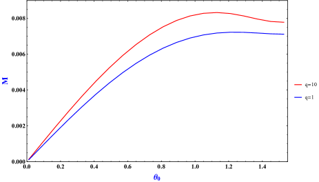
Figure 1: The mass parameter $M$ as a function of the embedding angle $\theta_{0}=\theta(u=1)$. The horizon is located at $u=1$ and the boundary is at $u=0$. From top to bottom $q=10$ and $q=1$, respectively.

In the new coordinates, the DBI action of the scalar field $\theta(u)$ is given by

$$S_{D7}=\int du~{}h(u)\frac{\cos^{3}\theta(u)}{u^{5}}\sqrt{1+u^{2}(1-u^{4})~{}\theta^{\prime}(u)^{2}}$$ (14)

One obtains the equation of motion

$$0 = \sin\theta(u)$$ (15)

$$\bigg{(}3u^{2}(u^{4}-1)(u^{q}+1)~{}\theta^{\prime}(u)^{2}-3(u^{q}+1)\bigg{)}$$

$$+u\,\cos\theta(u)$$

$$\bigg{(}\big{(}(q+1)~{}u^{q+4}-(q-3)~{}u^{q}+u^{4}+3\big{)}~{}\theta^{\prime}(u)$$

$$-u^{2}(u^{4}-1)\big{(}(q-2)~{}u^{q+4}-$$

$$(q-4)~{}u^{q}-2u^{4}+4\big{)}~{}\theta^{\prime}(u)^{3}$$

$$+u~{}(u^{4}-1)(u^{q}+1)~{}\theta^{\prime\prime}(u)\bigg{)}.$$

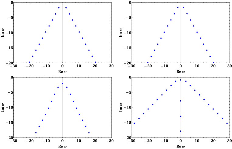
Figure 2: Massless quasinormal frequencies at vanishing momentum for $q=0$ (top-left), $q=1$ (top-right), $q=3$ (bottom-left), and $q=10$ (bottom-right). For $q=3$ a pure imaginary appears, and there is tower of these modes for $q=10$.

At $q=0$, it is similar to Kaminski:2009ce with a different definition of $\theta$ angle.

n	$Re(\omega_{n})$	$Im(\omega_{n})$
1	2.198814566	-1.759534627 i
2	4.211897203	-3.774888236 i
3	6.215543149	-5.777257013 i
4	8.217167238	-7.778080220 i
5	10.21806124	-9.778473884 i
6	12.21861770	-11.77869747 i
7	14.21899318	-13.77883893 i
8	16.21926141	-15.77893528 i
9	18.21946137	-17.77900453 i
10	20.2196154	-19.7790564 i
11	22.21974	-21.77910 i
12	24.220	-23.779 i
13	26.2	-25.8 i

Table 1: Thirteenth scalar massless QNMs computing by spectral method at $q=0$. We used 61 points in the grid which was judged by a comparison with a grid with 81 points.

The D7 brane embeddings are found by solving this differential equation from the horizon $u=1$ out to the boundary $u=0$. Black hole embedding is found by imposing boundary condition $\theta(1)=\theta_{0}$ and $\theta^{\prime}(1)=3\tan\theta_{0}/4$ on (15). Minkowski embedding is found by considering $\theta(u_{0})=\pi/2$ and $\theta^{\prime}(u_{0})\to\infty$.

Figure 1 shows the effect of $q$ on the D7 brane embeddings. In this figure, from top to bottom $q=10$ and $q=1$, respectively. To plot these curves, one chooses $\theta_{0}$ within interval $[0,\pi/2]$ and imposes a regularity condition on the horizon and shoots to the boundary. Then the quark mass $M$ can be read off from the near boundary behavior of the embeddings. It is clear from this figure that the mass $M$ is not a single-valued function of $\theta_{0}$. In the following figures, we decided to quote $\theta_{0}$ values instead of the mass parameter $M$. Since the region where $M$ is not single-valued implies an instability in the system which needs more investigations. Indeed the unstable modes that appear in figure 3 coincident with the change in the sign of $\frac{\delta M}{\delta\theta_{0}}$ in figure 1, qualitatively. There exist numerical issues for studying the limiting D7 brane embedding at $\theta_{0}=\pi/2$ so we consider a maximum value of $\theta_{0}=\pi/2-0.01$ in our paper.

In this paper, we are interested in fluctuations of the scalar field $\theta$ with mass squared $m^{2}=-3$. It is shown that the anomalous dimension plays a key role in the analysis of the QNMs. The fluctuations that we consider are space dependent and singlet states on S³ part of the D7 brane world volume. However, in the next section, we turn on an axial field in $\psi$ direction and investigate how it affects the scalar QNMs. We start the calculations by adding a time dependent fluctuation to the embedding with the following ansatz

$$\Theta(t,z,u)=\theta(u)+\vartheta(t,z,u),\,\,\,\,\,\,\psi=0.$$ (16)

By inserting the above fluctuation ansatz into the DBI action, one gets

$$S_{D7} = \int dt~{}du~{}h(u)~{}\frac{\cos^{3}\left(\Theta(t,z,u)\right)}{u^{5}}$$

$$\sqrt{1-\frac{u^{2}}{(1-u^{4})}~{}(\partial_{t}\vartheta(t,z,u))^{2}+u^{2}~{}(1-u^{4})~{}\Theta(t,z,u)^{2}},$$

where $\theta{(u)}$ is the solution of embedding equation of motion (15). Assuming plane wave form $\vartheta(t,z,u)=\text{e}^{-i\left(\omega\,t+k\,z\right)}\delta\theta(u)$ for the fluctuation, and keeping the equation of motion linearized, we find a second order differential equation for the fluctuation. In the following equation, we used (15) to eliminate $\theta^{\prime\prime}(u)$,

$$0 = \delta\theta^{\prime\prime}(u)+A_{1}(u)~{}\delta\theta^{\prime}(u)+A_{0}(u)~{}\delta\theta(u),$$ (18)

where

$$A_{0}(u) = \frac{1-u^{2}(-1+u^{4})~{}\theta^{\prime}(u)^{2}}{2u^{2}(-1+u^{4})^{2}}\sec^{2}\big{(}\theta(u)\big{)}$$

$$\bigg{(}-6(-1+u^{4})$$

$$+u^{2}\left(1+\cos\big{(}2\theta(u)\right)\big{)}\left((-1+u^{4})~{}k^{2}+\omega^{2}\right)\bigg{)}$$

$$A_{1}(u) = \dfrac{1}{u(-1+u^{4})(1+u^{q})}\big{(}-3-u^{4}+(-3+q)u^{q}$$

$$-(1+q)u^{4+q}+B(u)~{}\theta^{\prime}(u)^{2}\big{)}-6\theta^{\prime}(u)\tan\big{(}\theta(u)\big{)}$$

$$B(u) = -12u^{2}+18u^{6}-6u^{10}+3(-4+q)u^{2+q}$$

$$-6(-3+q)u^{6+q}+3(-2+q)u^{10+q}$$

The fluctuation equation (18) has two independent solutions $\delta\theta_{\pm}\equiv C_{\pm}(1-u)^{\pm i\omega/4}$. To impose ingoing boundary condition, we set $C_{+}=0$. The fluctuation function is then rescaled as $\delta\theta(u)\to(1-u)^{-i\omega/4}\tilde{\delta\theta}(u)$ to kill singularities. Using the spectral method, we solve (III) with appropriate boundary conditions. First, we consider the vanishing spatial momentum $k$

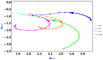
Figure 3: The first QNM in the complex frequency plane at vanishing spatial momentum $k$ as a function of the black hole embeddings using the spectral method. To explain each curve clearly, notice that there are two special points on each curve as starting $(\theta_{0}=0)$ and ending $(\theta_{0}=\pi/2)$ point. At each curve, arrow shows the direction of increasing $\theta_{0}$ along the curve. From left to right $q=1,0,3,10.$

and consider massless quarks $\theta_{0}=0$ corresponding to flat D7 brane embeddings. To do the calculations, we fix the temperature and vary the $q$ parameter. One should notice that in the dual theory, the meson spectrum is continuous and quarks are deconfined. Figure 2 shows the imaginary part of the first ten quasinormal mode frequencies as a function of the real part. In Table 1, we give the numerical values for $q=0$ case.

One finds that by increasing $q$ a massless pure imaginary mode appears in the spectrum. We checked carefully this new observation for different values of $q$ and found that there exists a critical value for $q_{c}$ around $2.705$ in which for a larger value of $q$ such modes appear in the system. By using the shooting method, these modes were not found in Hoyos-Badajoz:2006dzi . However, by changing the numeric method to the relaxation method, authors of Kaminski:2009ce found pure imaginary modes for massless modes. That is also interesting that one can not observe these modes by the spectral method. Moreover, Leaver method confirms the absence of a pure imaginary mode at $q=0$, too . It is a very interesting result that by increasing anomalous dimension $q$, a pure imaginary appears in massless modes for $q\approx 2.705$, actually a tower of these damping modes shows up for $q>3$ as we see in the bottom-right plot of figure 2.

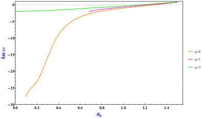
Figure 4: Pure imaginary QNMs at vanishing momentum as a function of the quark mass. The massless quark corresponds to ($\theta_{0}=0$) and for $q<q_{c}$ there is no pure imaginary mode for them. An instability occurs by changing the sign of the pure imaginary mode. From top to bottom $q=3,1,0.$

Next, we consider the first quasinormal frequencies of massive quarks in figure 3. This figure includes curves for different non-zero $q=1,0,3,10$ from left to right. We describe the curve for $q=0$, first. Zero quark mass $(\theta_{0}=0)$ corresponds to the point with the smallest value of the real part and by increasing the mass along the curve, the real part reaches a maximum value and then decreases to reach the endpoint. Also, the imaginary part turns by increasing $\theta_{0}$. Now we see in this figure how $q$ changes the general feature of the $q=0$ curve. For $q=3$, the general shape does not change but it moves slightly to right-hand side of the $q=0$ curve, while the $q=1$ curve moves left. But $q=3$ increases both the real part of complex frequency values, significantly and the imaginary turning point disappears. For $q=10$, the turning behavior along both the imaginary and real parts disappears. In contrast with the $q=3$ case, the absolute values of the imaginary part become smaller for $q=10$. One finds that the starting point (small mass) has been affected stronger than the endpoint (large mass) of each curve. It is an interesting observation that the effect of $q$ on the QNMs depends on the masses of quarks. Generally, the ordering of embeddings and QNMs for an arbitrary value of $\theta_{0}$ strongly depends on the value of $q$ whether $q<q_{c}$ or $q>q_{c}$. Perhaps it implies an interesting physics close to the critical value $q_{c}$.

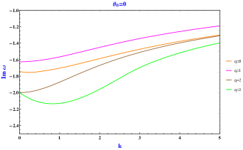
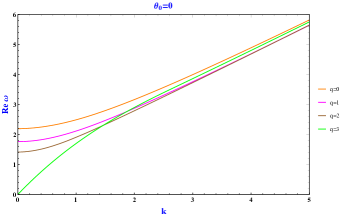
Figure 5: Dispersion relation for the first QNM for massless quarks $(\theta_{0}=0)$. As figure 2, for $q>2.705$ the real part of the mode vanishes at small momentum.

Figure 4 shows the behavior of the pure imaginary modes as a function of $\theta_{0}$ for different values of $q=0,1,3$ from bottom to top. As it was explained, there is no pure imaginary mode for massless ($\theta_{0}=0$) quarks with $q=0$ and $q=2$. It is clear from this figure that there exists a critical value for the quark mass in which the scalar QNM becomes tachyonic and makes the system unstable. Because the pure imaginary mode changes the sign from negative to positive. This behavior has been reported in Kaminski:2009ce for the massless quarks at $q=0$. They showed that this mode has an extraordinary large imaginary value for massless quarks. As it was mentioned this is not true if one uses Leaver or spectral method. Interestingly, one finds that by increasing $q$ the critical mass also decreases. Our study helps to understand better the behavior of the scalar massless QNM and confirms that it becomes tachyonic for massive quarks. So that the D7 brane embedding is not stable and one should find the true ground state of the system Kaminski:2009ce . We showed that considering the anomalous dimension leads to the appearance of the pure imaginary mode in the system. A new instability in AdS space-time with a scalar potential was found in Gursoy:2016ggq . Thermodynamics of Einstein-scalar field theories shows a rich structure Gursoy:2018umf . Dynamics near a first-order phase transition have been studied from holography in Bellantuono:2019wbn .

We presented the first QNM at vanishing spatial momentum $k$ in figure 2. Now we study the effect of non-zero $k$ by solving (III). We checked numerically that by increasing quark mass the real part shows a turning behavior similar to figure 3. We investigated the effect of the momentum of modes and found that by increasing $k$ the curves in the complex plane move to the right. As an important effect, we saw that $q_{c}$ grows by increasing $k$. Interestingly, the pure imaginary mode for massless quarks depends on the value of $k$ as well, we conclude that there is a critical value for momentum $k_{c}$ in which the pure imaginary mode disappears for $k>k_{c}$ at fixed $q$. For example, at $q=3$, we found that $k_{c}\approx 1$.

We show the dispersion relation for the first QNM for massless quarks in figure 5. The parameter $q$ is changing from $q=0$ to $q=1,2,3$ in this figure. By increasing spatial momentum $k$, the real part of the frequency increases and the mode gets more energy but at small $k$ one finds that the $q=3$ curve has a different behavior because, at zero spatial momentum, its real part is zero. This is the expected behavior that we learned from figure 2 where for larger $q$ a pure imaginary mode appears in the spectrum. the imaginary part of the mode in figure 5 confirms this behavior and describes the $q=3$ curve clearly. Modes with higher values of $k$ do not depend significantly on $q$ and move towards the $q=0$ curve.

IV Adding pseudoscalar field

We now switch on the pseudoscalar field $\psi$ on the world volume of the D7 brane. In the dual bulk gravity, we fluctuate the embedding D7 branes as

$$\Theta=\theta+\vartheta,\,\,\,\,\,\psi=\psi_{0}.$$ (19)

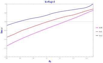
Figure 6: Pure imaginary QNM in the presence of pseudoscalar field $b$ at fixed value of $q=1$. From top to bottom $b=2,1,0$.

We checked that the equations of motion corresponding to the fluctuation of scalar and pseudoscalar decouple from each other like Bu:2018trt . Here, we ignore the fluctuation of the pseudoscalar similar to Ishigaki:2021vyv , where they perturbed the gauge and scalar fields. Also in Ishigaki:2020vtr fluctuations on pseudoscalar and gauge fields have been studied. Its interpretation from the AdS/CFT correspondence has been studied in Myers:2007we . One finds that near the boundary, on the world volume of the D7 brane embedding, the leading term in the expansion of this field determines the phase of the quark mass while the subleading term determines the expectation value of the related boundary operator.

We use the same simple ansatz as BitaghsirFadafan:2020lkh , which introduces the phase of quark mass as the following

$$\psi_{0}=bz$$ (20)

in which $b$ is an axial field and $z$ is one of the boundary field theory space directions. In the presence of a magnetic field, a similar ansatz has been considered in Kharzeev:2011rw ; Bu:2018trt and the chiral helix studied. As it was studied in BitaghsirFadafan:2020lkh , in the presence of an electric field, the $b$ field causes interesting transport due to the axial anomaly. In this paper, we take this ansatz and expect that our study could be related to such phenomena when the anomalous dimension of quark condensate has been added. Its study in QCD reveals topological Weyl Semimetal properties in quark-gluon plasma.

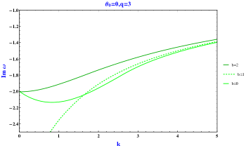
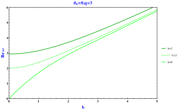
Figure 7: Effect of pseudoscalar field $b$ on the dispersion relation at fixed $q=3$. The value of $q$ is larger than $q_{c}$ and we consider zero quark mass $(\theta_{0}=0)$. From top to bottom $b=2,1,0$.

Our analysis is the same as the previous section and we will only show some of them. The fluctuations equation at finite momentum is given in Appendix A, too. Pure imaginary modes at vanishing spatial momentum and $q=1$ have been studied in figure 6. It shows that this mode depends strongly on the value of $b$. As it increases, the quark mass that triggers the instability decreases. We found the same structure at different values of $q$. We also found that there is no pure imaginary QNM for this case.

We extracted the effect of $b$ on the first QNMs in the complex plane of the frequency and found that at fixed $q$ they are similar to what we saw for $k$, i.e they move to the right when increasing $b$. Similarly, here there is a $b_{c}$ at which the massless pure imaginary mode disappears for $b>b_{c}$. As we checked, $b_{c}=1$ for $q=3$.

We obtain results for the dispersion relation in figure 7. It shows the first QNMs for massless quarks at $q=3$ in which momentum is changing from $k=0$ to $k=5$. At small $k$, the effect of $b$ is more clear than larger $k$ for both real and imaginary parts of the frequencies. Massive quarks show similar behavior, too. We find that for $q>q_{c}$, there is a crossing point for the imaginary part of the dispersion curves. For example, in this figure, the crossing point for $b=0$ and $b=1$ occurs at $k\approx 1.65$. Based on that, it is interesting to study the hydrodynamics of the system in the presence of the $b$ field.

V Summary

In this paper, we have studied an adapted D3/D7 brane setup that included a running anomalous dimension, $\gamma$, for the quark condensate. This allows us to describe the chiral restoration phase transition away from the phase of deconfined massive quarks. A nontrivial $h$ function has been considered as (3) with a free parameter $q$ that specifies the chiral symmetry breaking and anomalous dimension behavior in the theory. We explored the higher values of $q$ corresponding to the walking theories where the coupling constant changes slowly over a long range of energy scales.

The scalar flavor fields are $\theta$ and $\psi$ that describe transverse directions to the D7 brane embedding. In the dual picture, the scalar field $\theta$ is dual to the quark condensate and the phase transition occurs when the Breitenlohner Freedman (BF) bound is violated by the scalar field. For black hole D7 brane embedding, we studied the fluctuations of $\theta$ field at vanishing and finite spatial momentum, $k$. Our analysis shows that there is a critical $q_{c}$ about $2.705$ for massless quarks so that a new pure imaginary mode appears in the complex frequency plane. As an important observation, we found that the existence of such a mode depends on the value of momentum $k$ in the theory.

We can summarize the main results as follow:

• There is a critical mass for quarks in which the sign of the pure imaginary frequency changes and makes the system unstable.

• The critical mass is impressed by parameter $q$ and momentum $k$ so that it becomes smaller by increasing $q$ and gets larger by raising $k$.

The other main result of this paper was the effect of the pseudoscalar field $\psi$ on the QNMs of the scalar field. We take the simple ansatz $\psi=bz$ of BitaghsirFadafan:2020lkh where $b$ is an axial field and $z$ is one of the spatial boundary coordinates. In the presence of an electric field, one finds anomalous transport related to Weyl semimetals BitaghsirFadafan:2020lkh . We found that at small quark mass, the effect of the $b$ field is stronger than the massive ones. It is shown that $q_{c}$ increases also by increasing $b$ which is interesting from a phenomenological point of view. It is interesting to investigate possible effects on the melting of mesons in the QGP produced at LHC and RHIC. On the other hand, it could be related to topological phenomena like Weyl semimetal phases in condensed matter, but in QCD quarks have color degrees of freedom which make the phase space of the system much richer. It would also be interesting to generalize this study at finite density for scalar or vector fields.

Appendix A Fluctuation equation with axial $b$ field

In this appendix, we give the fluctuation equation at finite momentum in the presence of the pseudoscalar field $\psi(z)=bz$. Firstly, we give the embedding equation as

$$0 = b^{2}u^{3}\theta^{\prime}(u)^{2}\sin^{2}\big{(}\theta(u)\big{)}~{}\cos\big{(}\theta(u)\big{)}$$

$$\qquad\bigg{(}2+2u^{4}+(2-q)u^{q}+(2+q)u^{4+q}\bigg{)}$$

$$+(1+u^{q})\big{(}1+S(u)\big{)}\sin\big{(}\theta(u)\big{)}$$

$$\qquad\bigg{(}-1+u^{2}(-1+u^{4})\theta^{\prime}(u)^{2}\bigg{)}$$

$$+\frac{1}{2}~{}u~{}\cos\big{(}\theta(u)\big{)}$$

$$\qquad\Bigg{(}(6+2u^{4}+2(3-q)u^{q}+2(1+q)u^{4+q})\theta^{\prime}(u)$$

$$\qquad+u^{2}(-1+u^{4})\bigg{(}-8+4u^{4}-(8+2q)u^{q}$$

$$\qquad+(4-2q)u^{4+q}+b^{2}u^{2}~{}L(u)~{}\big{(}1-\cos\big{(}2\theta(u)\big{)}\big{)}\bigg{)}\theta^{\prime}(u)^{3}$$

$$\qquad-u(-1+u^{4})(1+u^{q})~{}S(u)~{}\theta^{\prime\prime}(u)\Bigg{)}.$$

Next we apply the fluctuation as $\Theta\equiv\Theta(t,z,u)=\theta(u)+\vartheta(t,z,u)$ where $\theta(u)$ is the solution of the embedding equation of motion (A). Then the DBI action reads as

$$S_{D7} = \int dt~{}du~{}h(u)~{}\frac{\cos^{3}\Theta}{u^{5}}$$

$$\sqrt{P~{}(\partial_{u}\Theta)^{2}+Q~{}(\partial_{z}\Theta)^{2}+W~{}\big{(}-1+u^{4}+u^{2}~{}(\partial_{t}\Theta)^{2}\big{)}},$$

where

$$P = -\frac{u^{2}}{2}(-1+u^{4})~{}S(u),$$

$$Q = u^{2},$$

$$W = -\big{(}1+b^{2}u^{2}\sin^{2}\Theta\big{)}.$$ (23)

Assuming plane wave form $\vartheta(t,z,u)=\text{e}^{-i(\omega t+kz)}\delta\theta(u)$ for the fluctuation, and keeping the equation of motion linearized, we find the fluctuation equation as

$$0 = \delta\theta^{\prime\prime}(u)+F~{}\delta\theta^{\prime}(u)+G~{}\delta\theta(u),$$ (24)

where

$$G = \frac{\big{(}1-u^{2}(-1+u^{4})~{}\theta^{\prime}(u)^{2}\big{)}~{}\sec^{2}(\theta(u))}{8u^{2}(-1+u^{4})~{}S(u)^{2}}~{}H$$

$$F = \dfrac{\sec(\theta(u))}{2u(-1+u^{4})(1+u^{q})~{}S(u)}~{}K$$

and

$$S(u) = 2+b^{2}u^{2}\bigg{(}1-\cos\big{(}2\theta(u)\big{)}\bigg{)}$$

also

$$H = 4(-1+u^{4})\big{(}-24+k^{2}(4+b^{2}u^{2})u^{2}$$

$$-u^{2}(22b^{2}-10b^{4}u^{2})\big{)}+2u^{2}(8+4b^{2}u^{2}+b^{4}u^{4})\omega^{2}$$

$$+u^{2}\cos\big{(}2\theta(u)\big{)}$$

$$\qquad\big{(}16(7b^{2}+k^{2}+3b^{4}u^{2})(-1+u^{4})$$

$$\qquad\qquad+(16-b^{4}u^{4})\omega^{2}\big{)}$$

$$+2b^{2}u^{2}\cos\big{(}4\theta(u)\big{)}$$

$$\qquad\big{(}-2(-1+u^{4})(-2+u^{2}(2b^{2}+k^{2}))$$

$$\qquad\qquad-u^{2}(4+b^{2}u^{2})\omega^{2}\big{)}$$

$$+b^{4}u^{6}\omega^{2}\cos\big{(}6\theta(u)\big{)}$$

$$+8b^{2}u^{3}(-1+u^{4})^{2}\theta^{\prime}(u)$$

$$\qquad\bigg{(}2\sin\big{(}2\theta(u)\big{)}+\sin\big{(}4\theta(u)\big{)}\bigg{)}$$

$$K = 4\cos\big{(}\theta(u)\big{)}~{}\big{(}-L(u)+2u^{4}(1+u^{q})\big{)}$$

$$+b^{2}u^{2}~{}\cos\big{(}3\theta(u)\big{)}$$

$$\qquad\big{(}2+2u^{4}+u^{q}(2-q+(2+q)u^{4})\big{)}$$

$$+\theta^{\prime}(u)(1+u^{q})\sin\big{(}\theta(u)\big{)}(-1+S(u))$$

$$+6u^{2}\theta^{\prime}(u)^{2}(-1+u^{4})\cos\big{(}\theta(u)\big{)}$$

$$\qquad\Bigg{(}-8+4u^{2}-2u^{q}(4-q+u^{4}(q-2))$$

$$\qquad+b^{2}u^{2}~{}L(u)\bigg{(}1-\cos\big{(}2\theta(u)\big{)}\bigg{)}\Bigg{)}$$

with

$$L(u) = -3+u^{4}+u^{q}\big{(}-3+u^{4}+q(-1+u^{4})\big{)}.$$

References

- (1) J. Casalderrey-Solana, H. Liu, D. Mateos, K. Rajagopal and U. A. Wiedemann, “Gauge/String Duality, Hot QCD and Heavy Ion Collisions,” doi:10.1017/CBO9781139136747 [arXiv:1101.0618 [hep-th]].
- (2) O. Aharony, S. S. Gubser, J. M. Maldacena, H. Ooguri and Y. Oz, “Large N field theories, string theory and gravity,” Phys. Rept. 323 (2000), 183-386 doi:10.1016/S0370-1573(99)00083-6 [arXiv:hep-th/9905111 [hep-th]].
- (3) P. Kovtun, D. T. Son and A. O. Starinets, “Viscosity in strongly interacting quantum field theories from black hole physics,” Phys. Rev. Lett. 94 (2005), 111601 doi:10.1103/PhysRevLett.94.111601 [arXiv:hep-th/0405231 [hep-th]].
- (4) K. B. Fadafan, “R**2 curvature-squared corrections on drag force,” JHEP 12 (2008), 051 doi:10.1088/1126-6708/2008/12/051 [arXiv:0803.2777 [hep-th]].
- (5) K. Bitaghsir Fadafan, “Charge effect and finite ’t Hooft coupling correction on drag force and Jet Quenching Parameter,” Eur. Phys. J. C 68 (2010), 505-511 doi:10.1140/epjc/s10052-010-1375-6 [arXiv:0809.1336 [hep-th]].
- (6) S. Grozdanov, N. Kaplis and A. O. Starinets, “From strong to weak coupling in holographic models of thermalization,” JHEP 07 (2016), 151 doi:10.1007/JHEP07(2016)151 [arXiv:1605.02173 [hep-th]].
- (7) M. Atashi, K. Bitaghsir Fadafan and G. Jafari, “Linearized Holographic Isotropization at Finite Coupling,” Eur. Phys. J. C 77 (2017) no.6, 430 doi:10.1140/epjc/s10052-017-4995-2 [arXiv:1611.09295 [hep-th]].
- (8) A. Karch and E. Katz, “Adding flavor to AdS / CFT,” JHEP 06 (2002), 043 doi:10.1088/1126-6708/2002/06/043 [arXiv:hep-th/0205236 [hep-th]].
- (9) J. Erdmenger, N. Evans, I. Kirsch and Threlfall, “Mesons in Gauge/Gravity Duals - A Review,” Eur. Phys. J. A 35 (2008), 81-133 doi:10.1140/epja/i2007-10540-1 [arXiv:0711.4467 [hep-th]].
- (10) D. Mateos, R. C. Myers and R. M. Thomson, “Holographic phase transitions with fundamental matter,” Phys. Rev. Lett. 97 (2006), 091601 doi:10.1103/PhysRevLett.97.091601 [arXiv:hep-th/0605046 [hep-th]].
- (11) C. Hoyos-Badajoz, K. Landsteiner and S. Montero, “Holographic meson melting,” JHEP 04 (2007), 031 doi:10.1088/1126-6708/2007/04/031 [arXiv:hep-th/0612169 [hep-th]].
- (12) P. K. Kovtun and A. O. Starinets, “Quasinormal modes and holography,” Phys. Rev. D 72 (2005), 086009 doi:10.1103/PhysRevD.72.086009 [arXiv:hep-th/0506184 [hep-th]].
- (13) K. Bitaghsir Fadafan, J. Cruz Rojas and N. Evans, “Deconfined, Massive Quark Phase at High Density and Compact Stars: A Holographic Study,” Phys. Rev. D 101 (2020) no.12, 126005 doi:10.1103/PhysRevD.101.126005 [arXiv:1911.12705 [hep-ph]].
- (14) M. Järvinen, “Holographic modeling of nuclear matter and neutron stars,” [arXiv:2110.08281 [hep-ph]].
- (15) P. Breitenlohner and D. Z. Freedman, Annals Phys. 144 (1982) 249. doi:10.1016/0003-4916(82)90116-6
- (16) M. Kaminski, K. Landsteiner, F. Pena-Benitez, J. Erdmenger, C. Greubel and P. Kerner, “Quasinormal modes of massive charged flavor branes,” JHEP 03 (2010), 117 doi:10.1007/JHEP03(2010)117 [arXiv:0911.3544 [hep-th]].
- (17) V. G. Filev, C. V. Johnson, R. C. Rashkov and K. S. Viswanathan, “Flavoured large N gauge theory in an external magnetic field,” JHEP 10 (2007), 019 doi:10.1088/1126-6708/2007/10/019 [arXiv:hep-th/0701001 [hep-th]].
- (18) M. Jarvinen and E. Kiritsis, “Holographic Models for QCD in the Veneziano Limit,” JHEP 03 (2012), 002 doi:10.1007/JHEP03(2012)002 [arXiv:1112.1261 [hep-ph]].
- (19) R. Alvares, N. Evans and K. Y. Kim, “Holography of the Conformal Window,” Phys. Rev. D 86 (2012), 026008 doi:10.1103/PhysRevD.86.026008 [arXiv:1204.2474 [hep-ph]].
- (20) L. Di Pietro and M. Serone, “Looking through the QCD Conformal Window with Perturbation Theory,” JHEP 07 (2020), 049 doi:10.1007/JHEP07(2020)049 [arXiv:2003.01742 [hep-th]].
- (21) T. DeGrand, “Lattice tests of beyond Standard Model dynamics,” Rev. Mod. Phys. 88 (2016), 015001 doi:10.1103/RevModPhys.88.015001 [arXiv:1510.05018 [hep-ph]].
- (22) A. Hasenfratz, C. Rebbi and O. Witzel, “Gradient flow step-scaling function for SU(3) with twelve flavors,” Phys. Rev. D 100 (2019) no.11, 114508 doi:10.1103/PhysRevD.100.114508 [arXiv:1909.05842 [hep-lat]].
- (23) D. Kutasov, J. Lin and A. Parnachev, “Holographic Walking from Tachyon DBI,” Nucl. Phys. B 863 (2012), 361-397 doi:10.1016/j.nuclphysb.2012.05.025 [arXiv:1201.4123 [hep-th]].
- (24) M. Jarvinen, “Holography and the conformal window in the Veneziano limit,” Int. J. Mod. Phys. A 32 (2017) no.36, 1747017 doi:10.1142/S0217751X17470170 [arXiv:1508.00685 [hep-ph]].
- (25) T. Alho, N. Evans and K. Tuominen, “Dynamic AdS/QCD and the Spectrum of Walking Gauge Theories,” Phys. Rev. D 88 (2013), 105016 doi:10.1103/PhysRevD.88.105016 [arXiv:1307.4896 [hep-ph]].
- (26) K. Bitaghsir Fadafan, W. Clemens and N. Evans, “Holographic Gauged NJL Model: the Conformal Window and Ideal Walking,” Phys. Rev. D 98 (2018) no.6, 066015 doi:10.1103/PhysRevD.98.066015 [arXiv:1807.04548 [hep-ph]].
- (27) U. Gürsoy, A. Jansen and W. van der Schee, “New dynamical instability in asymptotically anti–de Sitter spacetime,” Phys. Rev. D 94 (2016) no.6, 061901 doi:10.1103/PhysRevD.94.061901 [arXiv:1603.07724 [hep-th]].
- (28) U. Gürsoy, E. Kiritsis, F. Nitti and L. Silva Pimenta, “Exotic holographic RG flows at finite temperature,” JHEP 10 (2018), 173 doi:10.1007/JHEP10(2018)173 [arXiv:1805.01769 [hep-th]].
- (29) L. Bellantuono, R. A. Janik, J. Jankowski and H. Soltanpanahi, “Dynamics near a first order phase transition,” JHEP 10 (2019), 146 doi:10.1007/JHEP10(2019)146 [arXiv:1906.00061 [hep-th]].
- (30) J. P. Boyd (2000) ”Chebyshev and Fourier spectral methods” DOVER Publications, Inc.
- (31) P. Grandclement and J. Novak, “Spectral methods for numerical relativity,” Living Rev. Rel. 12 (2009), 1 doi:10.12942/lrr-2009-1 [arXiv:0706.2286 [gr-qc]].
- (32) A. Jansen, “Overdamped modes in Schwarzschild-de Sitter and a Mathematica package for the numerical computation of quasinormal modes,” Eur. Phys. J. Plus 132 (2017) no.12, 546 doi:10.1140/epjp/i2017-11825-9 [arXiv:1709.09178 [gr-qc]].
- (33) Y. Bu and S. Lin, “Holographic magnetized chiral density wave,” Chin. Phys. C 42 (2018) no.11, 114104 doi:10.1088/1674-1137/42/11/114104 [arXiv:1807.00330 [hep-th]].
- (34) S. Ishigaki, S. Kinoshita and M. Matsumoto, “Dynamical stability and filamentary instability in holographic conductors,” [arXiv:2112.11677 [hep-th]].
- (35) S. Ishigaki and M. Matsumoto, “Nambu-Goldstone modes in non-equilibrium systems from AdS/CFT correspondence,” JHEP 04 (2021), 040 doi:10.1007/JHEP04(2021)040 [arXiv:2012.01177 [hep-th]].
- (36) R. C. Myers, A. O. Starinets and R. M. Thomson, “Holographic spectral functions and diffusion constants for fundamental matter,” JHEP 11 (2007), 091 doi:10.1088/1126-6708/2007/11/091 [arXiv:0706.0162 [hep-th]].
- (37) K. Bitaghsir Fadafan, A. O’Bannon, R. Rodgers and M. Russell, “A Weyl semimetal from AdS/CFT with flavour,” JHEP 04 (2021), 162 doi:10.1007/JHEP04(2021)162 [arXiv:2012.11434 [hep-th]].
- (38) D. E. Kharzeev and H. U. Yee, “Chiral helix in AdS/CFT with flavor,” Phys. Rev. D 84 (2011), 125011 doi:10.1103/PhysRevD.84.125011 [arXiv:1109.0533 [hep-th]].