Unidirectional Thin Adapter for Efficient Adaptation of Deep Neural Networks

Abstract

In this paper, we propose a new adapter network for adapting a pre-trained deep neural network to a target domain with minimal computation. The proposed model, unidirectional thin adapter (UDTA), helps the classifier adapt to new data by providing auxiliary features that complement the backbone network. UDTA takes outputs from multiple layers of the backbone as input features but does not transmit any feature to the backbone. As a result, UDTA can learn without computing the gradient of the backbone, which saves computation for training significantly. In addition, since UDTA learns the target task without modifying the backbone, a single backbone can adapt to multiple tasks by learning only UDTAs separately. In experiments on five fine-grained classification datasets consisting of a small number of samples, UDTA significantly reduced computation and training time required for backpropagation while showing comparable or even improved accuracy compared with conventional adapter models.

1 Introduction

Deep neural networks (DNN) have shown outstanding performance in diverse fields and are developing rapidly. However, DNNs require a large amount of data to learn a target task. There has been a growing body of research that alleviates this issue by adapting a model pre-trained on a large dataset, such as ImageNet, to a small target dataset [1, 2]. The ‘pre-training followed by fine-tuning’ strategy is effective in improving performance for tasks of insufficient data. In particular, a few recent works propose minimizing or omitting the adaptation step by learning abundant knowledge from a large amount of data with large-scale models such as vision transformer (ViT) and DALL-E [3, 4].

However, large-scale DNNs require excessive computational resources for use on low-resource devices and are vulnerable to overfitting when fine-tuned with a small amount of data. Due to these issues, when adapting to new data in an environment with low computing power or insufficient data, many previous works freeze the backbone network and learn only the classifier using transfer learning or few-shot learning [2, 5].

Despite the aforementioned issues, the demand for learning or adapting DNNs in the low-resource environment, such as an edge device, is increasing. Training in the client device can improve the accuracy of the target task by further optimizing the pre-trained model with the target data of the user. We can extend this advantage to federated learning that improves a shared model without transferring private data by integrating only the training results of multiple client devices [6, 7]. In particular, in certain fields, such as fine-grained classification, adapting the pre-trained feature extractor layers to the target data is crucial because it is difficult to achieve high performance in such fields with only the features learned from a general dataset.

To train a DNN in a low-resource environment, it is essential to reduce the computational cost for learning. In previous work, diverse approaches have been proposed to reduce the size and computation of the DNN. Recently, there has been much progress to tackle this issue with lightweight models such as MobileNetV1 and V2 [8, 9], ShuffleNetV1 and V2 [10, 11], EfficientNetV1 and V2 [12, 13]. However, even with the lightweight models, training the entire model in a low-resource environment requires additional computation reduction.

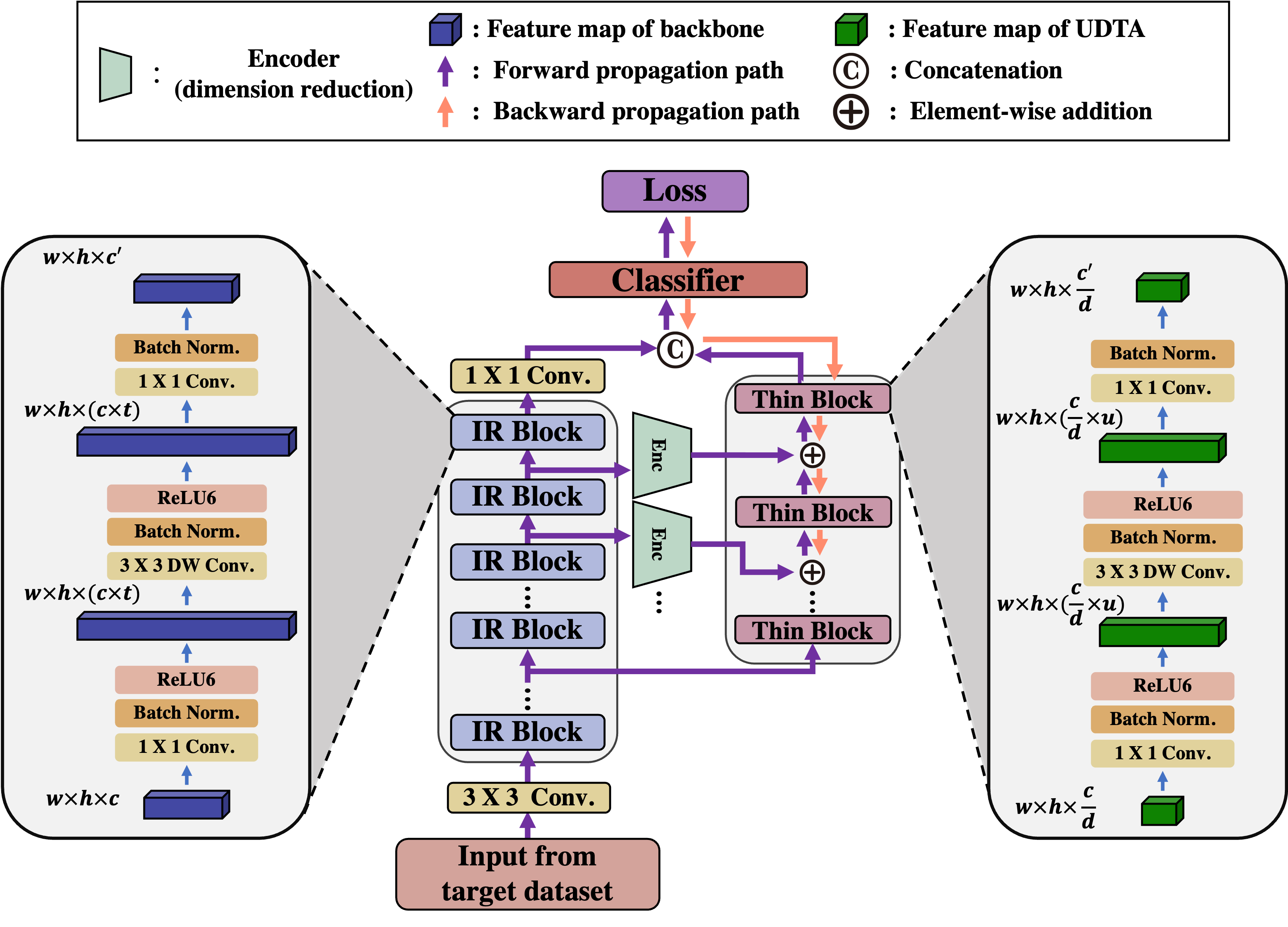
Figure 1: Unidirectional thin adapter (UDTA) combined with a backbone network (MobileNetV2). UDTA adapts the pre-trained backbone network by providing auxiliary features to complement the backbone features. Since the encoders reduce feature dimension, the thin blocks are substantially narrower than IR blocks.

On the other hand, a few previous studies have proposed adapter networks to learn DNNs with only a small amount of data [14, 15, 16, 17, 18]. The adapter improves performance by adjusting the activation of intermediate backbone layers or by providing complement features, without modifying the backbone substantially. Composed of a small number of parameters, the adapters are effective in reducing overfitting and preserving the pre-trained knowledge of the backbone. However, the existing adapters do not reduce computation for training because they still require the gradient of the backbone while training.

To overcome this limitation, in this paper, we propose a unidirectional thin adapter (UDTA) that adapts the pre-trained backbone network to the target task with minimal computation and a small number of target data. UDTA, as shown in Figure 1, is composed of thin and lightweight blocks that can be trained with minimal computation and a small amount of data.

Similar to the existing adapters, UDTA utilizes the intermediate features of the backbone to produce features effective for the target task. However, unlike conventional adapters, UDTA has only unidirectional connections from the backbone and does not transmit its features to the backbone. As a result, UDTA does not require the gradient of the backbone during backpropagation, thereby can be trained with minimal computation. In addition, we reduce the dimension of the feature maps delivered from the backbone by autoencoders, further reducing the size and computation of UDTA without significant loss of information. Since UDTA perfectly preserves the pre-trained knowledge of the backbone, a single backbone can conduct multiple tasks by combining a collection of per-task UDTAs. In experiments on five fine-grained classification datasets containing a small number of data, UDTA reduced the computation and time for backpropagation by 86.36% and 77.78% compared with model patches [14], while exhibiting comparable or improved accuracy compared with the other adapters.

Our main contributions include 1) a theoretical analysis of the reason why the existing adapter networks fail to reduce computation for training, 2) a novel unidirectional thin adapter (UDTA) to adapt a pre-trained DNN to a new dataset with minimal computation and data, 3) a lightweight adapter structure and reduced data transfer due to dimensionality reduction, and 4) comparable or improved accuracy compared with existing adapter networks for five small-size datasets for fine-grained classification.

Section 2 of this paper introduces related work. Section 3 analyzes the problems with conventional adapter networks in terms of computational efficiency in backpropagation and proposes the unidirectional thin adapter to overcome the limitation. Section 4 and Section 5 present experimental results and conclusions, respectively.

2 Related Work

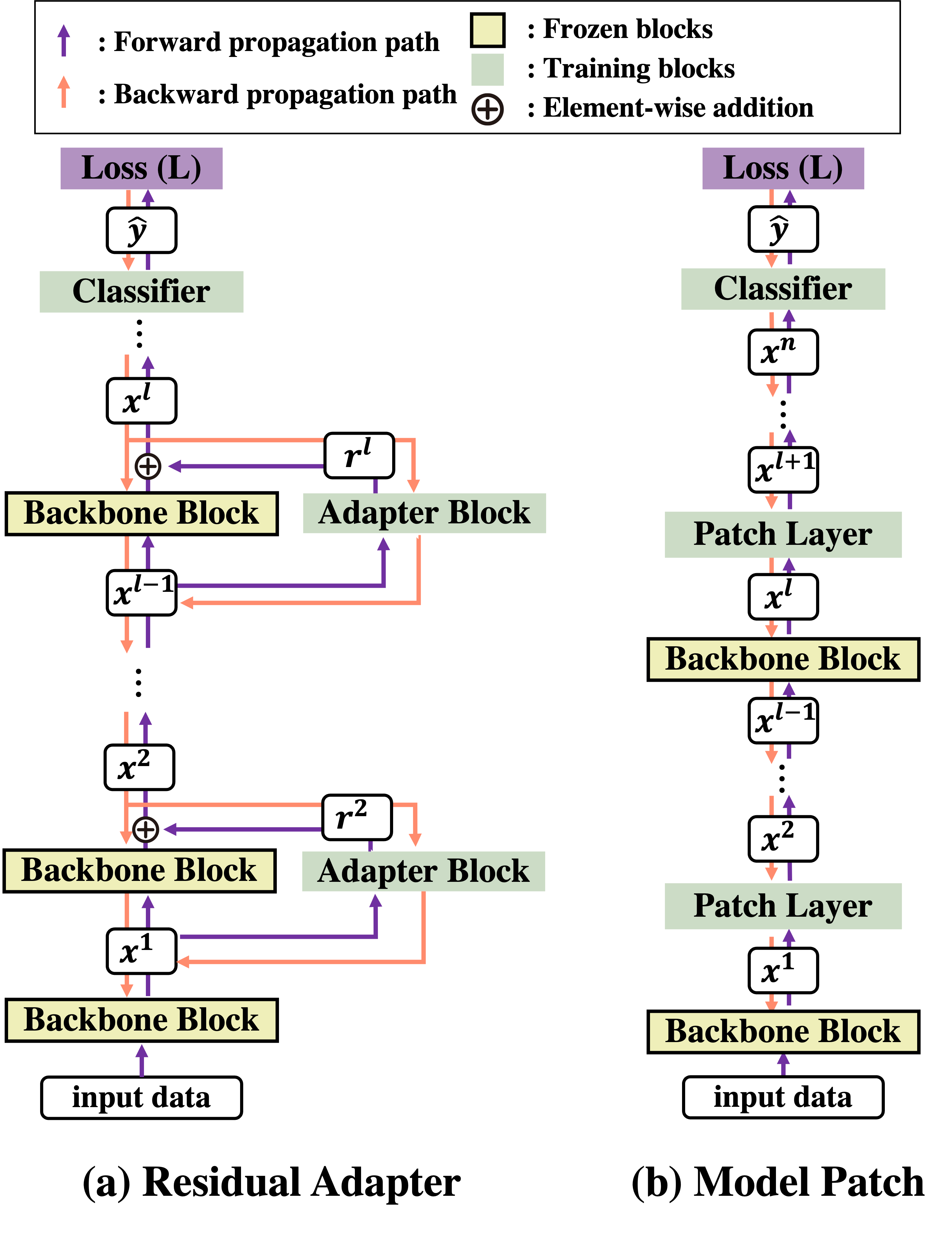
Figure 2: Training of residual adapters and model patches. The red arrows illustrate the backpropagation flow. Both adapters require the gradient of the backbone blocks.

Pre-training followed by fine-tuning strategy In recent years, there has been an increasing interest in domain adaptation by fine-tuning a pre-trained DNN model. Specifically, the ‘pre-training followed by fine-tuning’ strategy, that first pre-trains a DNN with a large volume of data, such as ImageNet, and then fine-tunes it with a small amount of target data, has been widely adopted and demonstrated its effectiveness in improving performance for the tasks with insufficient training data. [2] proposes a meta transfer learning method for effectively fine-tuning a DNN pre-trained on a large dataset for multiple few-shot tasks. [5] applies a pre-trained convolutional neural network (CNN) to map samples to a latent space, and then classifies the latent feature using a simple model, such as k-NN classifier and Gaussian mixture models.

Lightweight network models MobileNetV2 [9], ShuffleNetV2 [11], and EfficientNetV2 [13] propose lightweight DNN models with reduced size and computation. TinyTL [19] proposes a memory-efficient model that learns only the bias without storing intermediate activation. Besides the above models, researchers have attempted to reduce the computation or the number of parameters of the DNN. Lightlayers [20] and batch ensemble [21] propose network modules as to reduce computation. Lightlayers decompose convolutional layers and fully connected layers into a combination of minor operations. In contrast, batch ensemble approximates a weight matrix by the product of a single row and a single column.

We built our backbone network based on MobileNetV2 [9]. The main building block of MobileNetV2 is the inverted residual (IR) block that was designed to minimize computational requirement and the number of parameters preserving performance. The IR block is composed of a 1x1 convolution that increases the number of channels, a 3x3 depth-wise convolution, and another 1x1 convolution that decreases the number of channels. The third 1x1 convolution layer omits ReLU activation to reduce information loss.

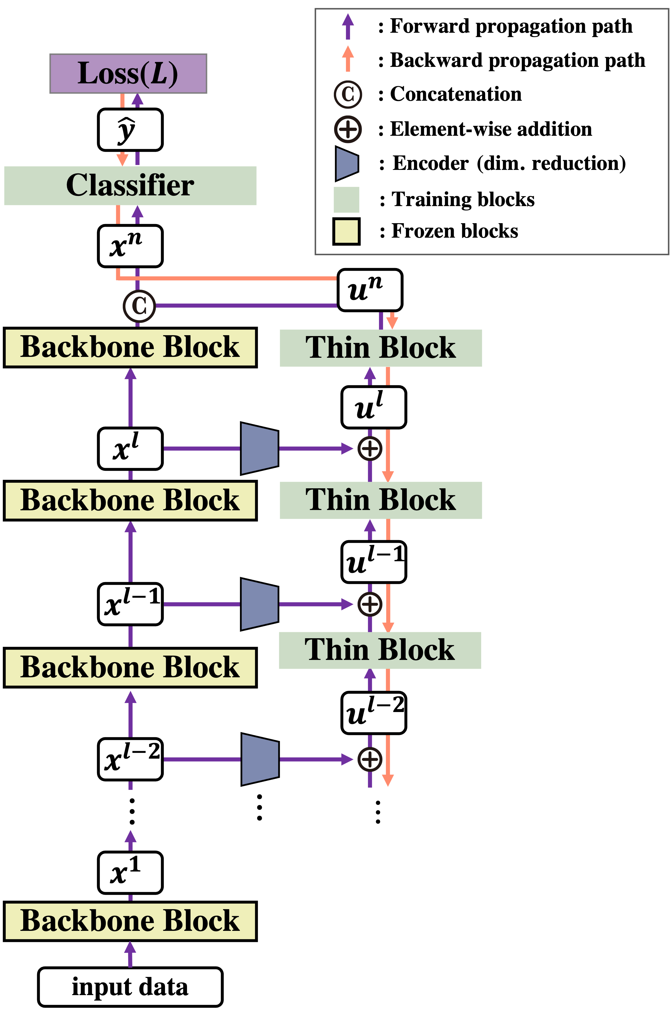
Figure 3: Training of UDTA. The red arrows illustrate the backpropagation flow. UDTA learns without the gradient of the backbone.

Adapter networks Numerous previous studies on domain adaptive learning have proposed adapter networks to adapt a pre-trained DNN to a new target domain efficiently [22, 14, 15, 16, 17, 18]. Composed of a small number of parameters, the adapter networks can be trained with a small number of target data.

Some previous works have applied partial learning to reduce the number of parameters [22, 14]. [14] proposes to adapt a pre-trained DNN to a new task by learning only a small number of layers, fixing the other parts. They demonstrate that training only a few layers with a small number of parameters, such as scale-and-bias patch and depthwise-convolution patch, can significantly improve performance for a new target task. [15, 16] proposes a residual adapter that reduces the number of parameters to train in domain adaptation. While [14] reuses the layers of the pre-trained network for model patches, [15, 16] adapt the backbone by combining it with a collection of adapter networks and learning only the adapters. The adapter network is composed of layers with a small number of parameters, such as 1x1 convolution and batch normalization. They combine residual adapters to all 3x3 convolution layers of the backbone network. Model patches and residual adapters help DNNs adapt to a new domain with a small number of training samples. However, they do not reduce the computational cost for training, as analyzed in the next section.

[17, 18] propose a budget-aware adapter ($BA^{2}$) and FLUTE to reduce the computational cost. Budget-aware adapter selects the most relevant feature channels and saves the computational cost by activating only the selected channels. [18] proposes a method for few-shot learning with a universal template (FLUTE), a partial model that can define a wide array of dataset-specialized models by plugging in appropriate components. They are effective in reducing computation for forward propagation, but cannot be used to reduce computation for training.

3 Efficient Domain Adaptation with Unidirectional Thin Adapter

3.1 Backpropagation of Conventional Adapter Networks

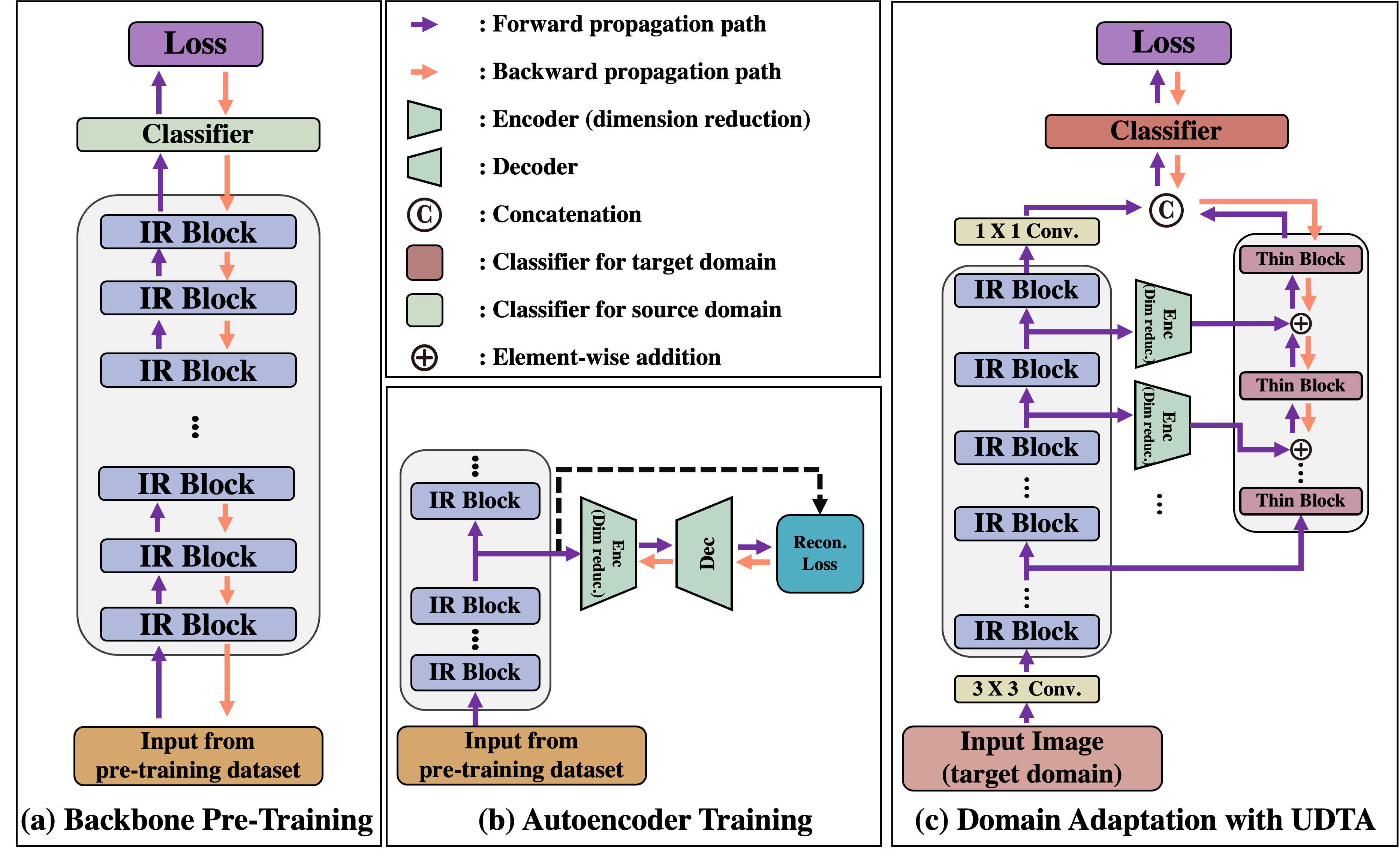
Figure 4: Training of UDTA. (a) and (b) are conducted on a server, while (c) is conducted on the client device.

The gradient descent algorithm optimizes the neural network by adjusting model parameters to minimize loss function as Eq. (1), where $w^{l}$, $L$, and $\eta$ denote the weights of the $l$-th layer, loss function, and learning rate, respectively.

$$w^{l}\leftarrow w^{l}-\eta\frac{\partial L}{\partial w^{l}}$$ (1)

As shown in Eq. (1), the gradient descent algorithm requires the gradient $\frac{\partial L}{\partial w^{l}}$. The backpropagation algorithm computes the gradient sequentially from the top to the bottom layer.

Residual adapters are combined with the backbone layers in a parallel or serial way. Figure 2(a) displays parallel residual adapters attached to the backbone network. In training procedure, the backbone blocks are fixed and only the adapter blocks are trained with the target data. To train the weights of the residual adapter $w_{r}^{l}$, we need to compute its gradient $\frac{\partial L}{\partial w_{r}^{l}}$.

The red arrows in Figure 2(a) illustrate the backpropagation path to learn the residual adapters. Applying the chain rule, $\frac{\partial L}{\partial w_{r}^{l}}$ is decomposed as Eq. (2), where $x^{l}$ and $r^{l}$ denote activation of the $l$-th block in the backbone and the residual adapter, respectively.

$$\frac{\partial L}{\partial w_{r}^{l}}=\frac{\partial L}{\partial r^{l}}\frac{\partial r^{l}}{\partial w_{r}^{l}}=\frac{\partial L}{\partial x^{l}}\frac{\partial x^{l}}{\partial r^{l}}\frac{\partial r^{l}}{\partial w_{r}^{l}}$$ (2)

$\frac{\partial L}{\partial x^{l}}$ in Eq. (2) is computed by combining the gradient from $x^{l+1}$ and that from $r^{l+1}$ as Eq. (3). The recursive expansion of Eq. (3) includes $\frac{\partial L}{\partial x^{n}}(\prod_{k=l}^{n-1}\frac{\partial x^{k+1}}{\partial x^{k}})$.

$$\frac{\partial L}{\partial x^{l}}=\frac{\partial L}{\partial x^{l+1}}\frac{\partial x^{l+1}}{\partial x^{l}}+\frac{\partial L}{\partial r^{l+1}}\frac{\partial r^{l+1}}{\partial x^{l}}$$ (3)

As shown in Eq.(2) and (3), computing $\frac{\partial L}{\partial w_{r}^{l}}$ requires the gradients $\frac{\partial L}{\partial x^{k}}$ for all $k\geq l$. Consequently, training the parallel residual adapter requires backpropagation through the entire network including the backbone. The computation of the gradients to learn serial adapters is similar to that with model patches explained below.

Figure 2(b) illustrates the forward and backward propagation of a DNN with model patches. The gradient for the weight $w_{p}^{l}$ of the $l$-th patch layer is computed as Eq.(4), where $x^{l}$ is the activation of a patch layer and $x^{k}$s are the activation of either a patch layer or a backbone layer.

$$\frac{\partial L}{\partial w_{p}^{l}}=\frac{\partial L}{\partial x^{l}}\frac{\partial x^{l}}{\partial w_{p}^{l}}=\frac{\partial L}{\partial x^{n}}(\prod_{k=l}^{n-1}\frac{\partial x^{k+1}}{\partial x^{k}})\frac{\partial x^{l}}{\partial w_{p}^{l}}$$ (4)

Eq. (4) shows that the training of model patches also requires backpropagation through the entire network.

3.2 Structure of Unidirectional Thin Adapter

Figure 1 illustrates the structure of UDTA combined with a backbone network. In Figure 1, $w$, $h$, and $c$ denote the width, height, and the number of channels of the backbone feature map, respectively. $d>1$, $t>1$ and $u>1$ denote the dimensionality reduction factor of the encoder, channel expansion factor of the IR block, and channel expansion factor of thin block, respectively.

The backbone network is pre-trained with a large-scale dataset and extracts high-level features from the input. The UDTA is composed of a stack of thin blocks. The dimension of the UDTA feature map is lower than that of the backbone feature map at the same level. Each thin block takes as input the feature map of the corresponding backbone block, and propagates features to upper blocks to produce auxiliary features for the classifier. In training, we freeze the backbone and train only UDTA with the target data to produce auxiliary features that complement the backbone features, thereby improving the performance for the target task. In other words, the backbone learns general knowledge from a large-scale pre-training dataset, while UDTA learns domain-specific knowledge from the target data to complement the backbone features. The classifier combines the features from the backbone and UDTA and outputs the classification result.

The encoders between the backbone and the UDTA blocks reduce the dimension of the features transmitted from the backbone, which allows further reducing the size and computation of UDTA. We use autoencoders to train UDTA encoders to reduce feature dimension while minimizing information loss. As a result, the UDTA comprises a small number of parameters and requires a small amount of computation for both forward and backward propagation.

The full training of the entire network requires a large amount of computation. On the other hand, freezing the backbone and training only the classifier reduce computation significantly but exhibit limited performance because of the lack of domain-specific knowledge. UDTA can make a good trade-off between performance and computational cost. In addition, UDTA perfectly preserves the pre-training knowledge of the backbone since it learns without modifying the backbone. Therefore, it is possible to perform multiple tasks with a single backbone network by adapting only UDTAs to the target tasks. This is an important advantage, especially in the low-resource environment.

The most prominent advantage of UDTA over existing adapter networks is that we can train it with a minimal amount of computation. In Section 3.1, we have shown that residual adapters and model patches cannot reduce computation for training, because training them requires the gradient of the backbone which demands heavy computation. To learn without the gradient of the backbone, we designed UDTA to be connected to the backbone in only one direction. While it receives the intermediate features from multiple backbone blocks, it does not provide any feature to the backbone blocks.

Training UDTA requires the gradient $\frac{\partial L}{\partial w_{u}^{l}}$, where $w_{u}^{l}$ denotes the weights of the $l$-th thin block. The gradient is computed as Eq. (5).

$$\frac{\partial L}{\partial w_{u}^{l}} =\frac{\partial L}{\partial u^{l}}\frac{\partial u^{l}}{\partial w_{u}^{l}}=\frac{\partial L}{\partial u^{n}}\frac{\partial u^{n}}{\partial u^{l}}\frac{\partial u^{l}}{\partial w_{u}^{l}}$$ (5)

$$=\frac{\partial L}{\partial u^{n}}(\prod_{k=l}^{n-1}\frac{\partial u^{k+1}}{\partial u^{k}})\frac{\partial u^{l}}{\partial w_{u}^{l}}$$

Note that Eq. (5) does not require the gradient of the backbone $\frac{\partial L}{\partial x^{l}}$ for any $l$. Figure 3 illustrates the backpropagation path to compute gradient $\frac{\partial L}{\partial w_{u}^{l}}$ to train UDTA. The red arrow starts from the loss and goes through the thin blocks. However, it does not pass any backbone block. Consequently, UDTA can learn without backpropagation through the entire backbone network, and therefore, can save computation for training substantially.

The structure of UDTA is based on the inverted residual block [9], as shown in Figure 1. The first $1\times 1$ convolution increases the number of channels, and the $3\times 3$ depth-wise convolution extracts spatial information from the input feature. The last 1 × 1 convolution decreases the number of channels. The width and depth of UDTA can be flexibly decided according to the characteristics of the target data and the backbone network. The autoencoder combines an encoder and a decoder, each of which is composed of a $1\times 1$ convolution layer. The input dimension of the autoencoder is the same as the output dimension of the backbone layer, while its hidden dimension is the same as the input dimension of the UDTA layer.

3.3 Learning of Recognition System Using Unidirectional Thin Adapter

We train the entire network in three steps. In the first step, the backbone network learns abundant general knowledge that is useful for many target tasks, from a large-scale dataset such as ImageNet on a server, as shown in Figure 4(a).

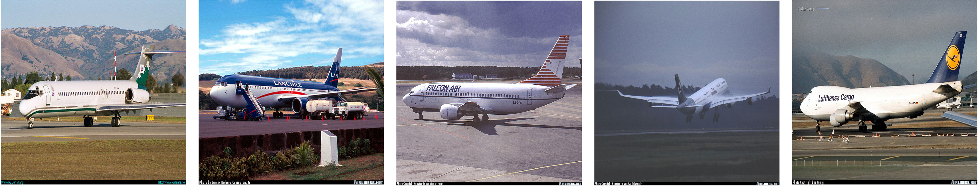
Figure 5: FGVC-Aircraft image samples. Only minor differences distinguish the aircraft types.

Table 1: The number of classes and samples in the datasets for fine-grained classification. (Air: FGVC-Aircraft, Cars: Stanford Cars, DTD: Describable Textures, Dogs: Stanford Dogs, Flow: Flowers-102)

	Classes	Training Samples	Test Samples	Total Samples
Air	100	6,667	3,333	10,000
Cars	196	8,144	8,041	16,185
DTD	47	3,760	1,880	5,640
Dogs	102	2,040	6,149	8,189
Flow	120	12,000	8,580	20,580

Table 2: Experimental settings for backbone pre-training, autoencoder training, and domain adaptation

	Epoch	Learning rate	Batch	Optimizer	Loss function
Pre-training	120	0.01	256	ADAM (a=0.9, b= 0.999)	Cross Entropy
AE training	120	0.001	256	ADAM (a=0.9, b= 0.999)	MSE
Domain adap.	120	0.001	256	ADAM (a=0.9, b= 0.999)	Cross Entropy

The second step is to learn the encoders for dimensionality reduction. Similar to the first step, we also train the autoencoder with a large-scale pre-training dataset on a server, as shown in Figure 4(b). To reduce feature dimension while minimizing the loss of information, we train the autoencoder by the $L_{2}$ reconstruction loss. We do not train the backbone and the autoencoders at the same time because, before the backbone training is complete, learning to compress the immature features is meaningless. After the second step, we use the encoder for dimensionality reduction and discard the decoder.

In the final step, we freeze the backbone and autoencoder, and train only UDTA and the classifier with the target dataset. Due to the encoder, the feature map of UDTA has significantly lower dimension compared with that of the backbone, and therefore, UDTA can learn from a small amount of data with a minimal amount of computation. Furthermore, we combine only a few top layers with thin layers, further saving parameters and computation. However, for the backbone block with low dimensionality, we directly connect the thin block to the backbone block without encoder.

4 Experiment

4.1 Datasets and Experimental Settings

Datasets We used the ImageNet dataset [23] for the pre-training of the backbone network and the autoencoders. For the target data, we used five small-size datasets designed for fine-grained classification: FGVC-Aircraft [24], Stanford Cars [25], DTD [26], Oxford 102 Flowers [27], and Stanford Dogs [28] datasets. They consist of a small number of samples per class, and the difference between class images in those datasets is small compared with ordinary datasets. Figure 5 displays a few samples in FGVC-Aircraft set. To obtain high performance for those datasets, it is essential to learn discriminative features by domain adaptation. The number of classes and samples are presented in Table 1.

Table 3: Computation, time, and accuracy of UDTA compared with other models. (Scratch: backbone trained from scratch, Full-FT: fully fine-tuned backbone, Top-FT: backbone with fine-tuned top layer, MP: model patch [14], RA: residual adapters [15, 16], and UDTA: proposed method)

	F.FLOPs	B.FLOPs	F.Time	B.Time	Acc.	Params
Scratch	85,322M	170,645M	8.2ms	12.6ms	63.57	2352K
Full-FT	85,322M	170,645M	8.2ms	12.6ms	81.03	2352K
Top-FT	85,322M	66M	7.8ms	0.4ms	41.91	129K
MP	85,322M	165,096M	8.2ms	11.7ms	66.17	156K
RA	92,611M	171,966M	10.4ms	12.0ms	62.19	163K
UDTA	97,357M	22,499M	9.7ms	2.6ms	67.56	865K

Experimental Environment and Settings We conducted experiments on a PC with RTX-3090 GPU, AMD Threadripper 1900x CPU, and 32GB of RAM. We implemented the models on Ubuntu Linux using PyTorch (1.7.1v) and Torchvision (0.8.2v). The experimental settings and hyper-parameters are presented in Table 2.

Metrics We measured classification performance by top-1 accuracy on the test data, the amount of computation by FLOPs (floating point operations), and time by msec. In each table, F.FLOPs and B.FLOPs denote the computation for forward and backward propagation, and F.Time and B.Time denote the time for forward and backward propagation, respectively. Additionally, we present the number of parameters to train in each model.

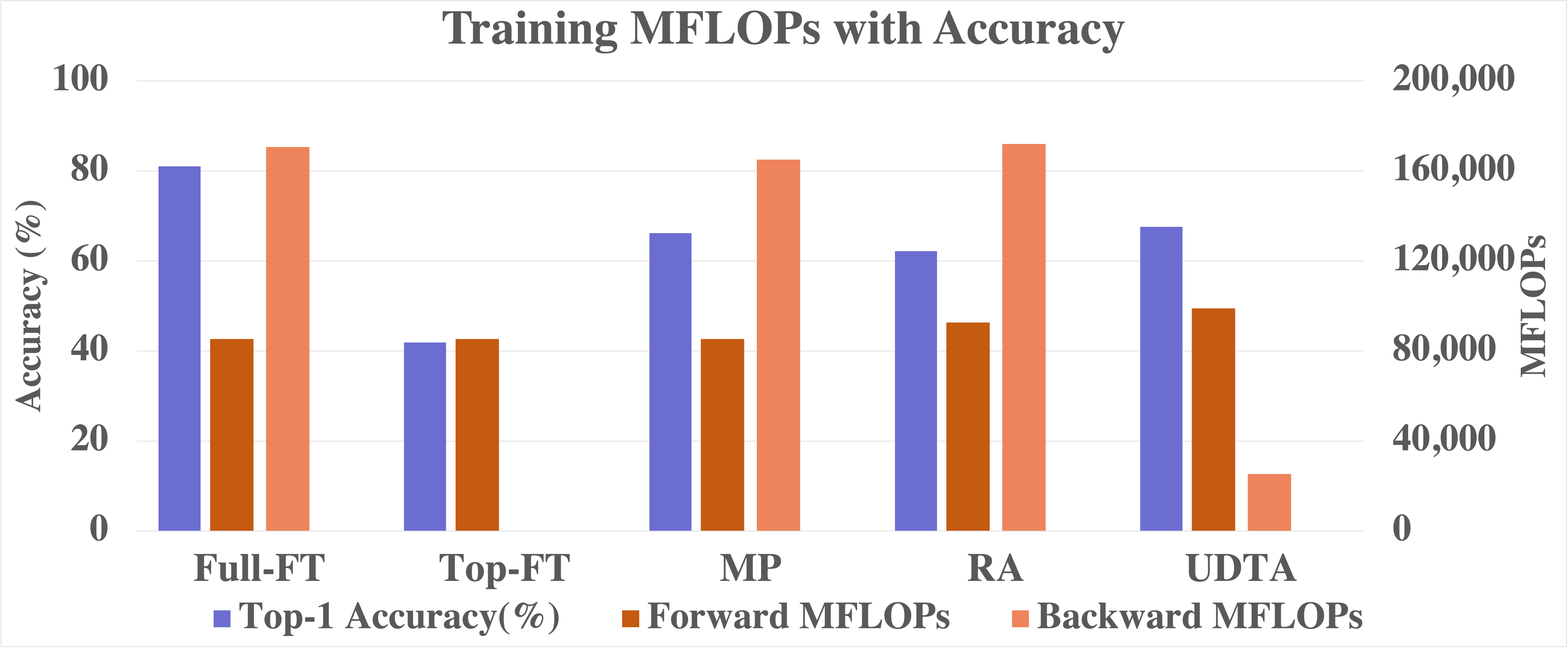
(a) Accuracy (blue), computation for forward propagation (red) and backpropagation (orange)

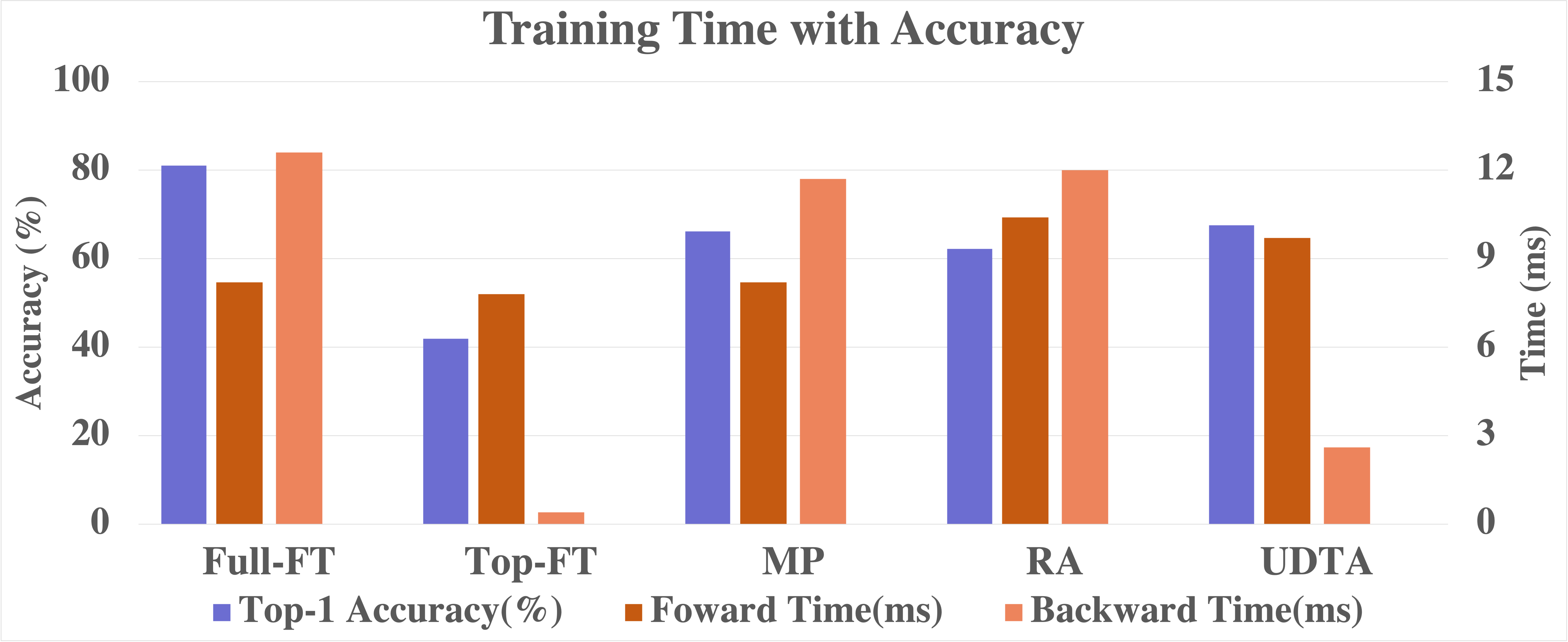
(b) Accuracy (blue), time for forward propagation (red) and backpropagation (orange)

Figure 6: Accuracy, computation, and time for forward/backward propagation of UDTA compared with other models

4.2 Comparison with Other Adapter Networks

In the first experiment, we compared UDTA with five other models on the FGVC-Aircraft dataset. The experimental results are presented in Table 3 and Figure 6, where ‘Scratch’ denotes the backbone network only trained with the target datasets from scratch, ‘Full-FT’ denotes the backbone pre-trained with ImageNet and then fully fine-tuned with the target dataset. ‘Top-FT’ is the backbone network in which only the top layer was fine-tuned after pre-training. ‘MP’, ‘RA’, and ‘UDTA’ denote model patch, residual adapter, and the proposed adapter, respectively.

Without pre-training, the backbone trained from scratch (‘Scratch’) was slow and exhibited a poor accuracy. The full fine-tuning of the pre-training backbone (‘Full-FT’) exhibited the best accuracy but required heavy computation for backpropagation. On the other hand, fine-tuning only the top layer of the pre-trained backbone (‘Top-FT’) was the fastest but exhibited the lowest accuracy. Applying model patches (‘MP’) and residual adapters (‘RA’) improved accuracy compared with the ’TOP-FT’ model with learning a minimal number of parameters. However, they have little effect in reducing the computation and time for training. The proposed model, UDTA, exhibited higher accuracy than other adapters, while reducing the computation and time for backward propagation by 86.36% from 165,096 MFLOPs to 22,499 MFLOPs, and 77.78% from 11.7 msec to 2.6 msec compared with model patches. In return, UDTA increased the computation and time for forward propagation by 15.88% and 18.29%, respectively.

Table 4: Computation, time, and accuracy according to the number of thin blocks B

B.	F.FLOPs	B.FLOPs	F.Time	B.Time	Acc.	Params
1	91,364M	12,148M	8.2ms	1.3ms	65.01	634K
3	97,357M	22,499M	9.7ms	2.6ms	67.56	865K
5	102,138M	30,782M	11.1ms	3.7ms	63.51	1002K
7	113,233M	51,870M	11.7ms	4.3ms	60.24	1007K

Table 5: Computation, time, and accuracy according to expansion factor $u$

$u$	F.FLOPs	B.FLOPs	F.Time	B.Time	Acc.	Params
2	90,475M	8,570M	8.8ms	2.1ms	60.06	433K
4	94,674M	16,967M	9.3ms	2.5ms	65.22	705K
6	97,357M	22,499M	9.7ms	2.6ms	67.56	865K
8	103,072M	33,763M	9.8ms	3.3ms	67.56	1249K

Table 6: Domain adaptation performance (Top-1 accuracy) on multiple datasets

	Air	Cars	DTD	Dogs	Flow
Scratch	63.57%	72.80%	39.94%	55.65%	59.39%
Full-FT	81.03%	88.62%	69.14%	82.59%	95.65%
TOP-FT	41.91%	50.20%	67.44%	80.17%	90.82%
MP	66.17%	76.33%	68.61%	81.62%	93.78%
RA	62.19%	74.94%	67.58%	77.87%	92.60%
UDTA	67.56%	81.21%	69.89%	79.94%	93.54%

To find the optimal depth and width of UDTA, we measured computation, time, and accuracy on the FGVC-Aircraft dataset changing the number of thin blocks and the expansion factor $u$ in Figure 1. The results are presented in Table 4 and 5. As the width and depth of UDTA increased, the amount of computation and time increased. The accuracy increased with width but was not proportional to depth. We found the optimal size of UDTA, in terms of the trade-off between computation and accuracy, with depth three and expansion factor six.

We also evaluated UDTA and existing models on multiple fine-grained classification datasets. Table 6 measures the accuracy of the models. The ‘Full-FT’ model exhibited the highest accuracy. The accuracy of UDTA was comparable or higher than the other adapter networks.

5 Conclusion

We analyzed why conventional adapter networks fail to reduce the amount of computation for training and proposed a unidirectional thin adapter (UDTA) for efficient domain adaption of the DNN. UDTA improves the performance for the target task by providing auxiliary features to complement the features of the backbone network, which was trained from a general pre-training dataset. Unlike conventional adapter networks, UDTA is connected to the backbone network in one way, not requiring the gradient of the backbone network for training, which substantially reduces computation for backpropagation. In experiments on five small-size datasets for fine-grained classification, UDTA reduced the amount of computation and time for backpropagation by 86.36% and 77.78%, respectively, compared with model patches [14], while exhibiting comparable or even improved accuracy.

Appendix A Training procedure

The training of UDTA is composed of three steps: pre-training step, autoencoder training step, and domain adaptation step.

1. Pre-train the backbone network using the source dataset which consists of a large amount of image data.

2. Train the autoencoders using the source dataset. Each autoencoder is trained by the output features of the backbone network blocks which are connected to the autoencoders.

3. Adapt the image recognition model(backbone network + encoder + UDTA) to a new domain using fine-grained classification dataset

   1. Connect UDTA to the backbone network by the encoder.

   2. Train UDTA for domain adaptation while freezing the backbone network blocks.

Algorithm 1 Pre-training algorithm

Source dataset: $X_{s}=\{x_{s}^{1},x_{s}^{2},...x_{s}^{n}\}$ where $n$ is the total number of the source data

Class labels of source dataset: $Y_{s}=\{y_{s}^{1},y_{s}^{2},...y_{s}^{n}\}$

Batch size: $m$

Backbone network parameters: $\theta_{b}$

Classification loss function: $L$

Learning rate: $\eta$

for $i=1$ to number of epochs do

     for $j=1$ to $n/m$ do

         Sample $m$-size batch from $X_{s}$

         $k$ is the index of the data in the batch

         Gradient $\hat{g}\leftarrow\frac{1}{m}\nabla_{\theta_{b}}\Sigma_{k}L(f(x_{s}^{k};\theta_{b}),y_{s}^{k})$

         $\theta_{b}\leftarrow\theta_{b}-\eta\hat{g}$

     end for

end for

Algorithm 2 Autoencoder training algorithm

Source dataset: $X_{s}=\{x_{s}^{1},x_{s}^{2},...x_{s}^{n}\}$ where $n$ is the total number of the source data

List of parameters of autoencoders: $\Theta_{AE}=\{\theta_{ae}^{1},\theta_{ae}^{2},...\theta_{ae}^{h}\}$ where $h$ is the number of autoencoders

Batch size: $m$

Backbone network parameters: $\theta_{b}$

Reconstruction loss function: $L_{rec}$

Learning rate: $\eta$

for $i=1$ to number of epochs do

     for $j=1$ to $n/m$ do

         Sample $m$-size batch from $X_{s}$

         $k$ is the index of the data in the batch

         for $l=1$ to $h$ do

              $o^{l}(x_{s}^{k};\theta_{b})$ is the $l$-th output feature of backbone network starting from the first block connected to the autoencoder

              $f(o^{l}(x_{s}^{k};\theta_{b});\theta_{ae}^{l})$ is the output of $l$-th autoencoder

              Gradient $\hat{g}^{l}\leftarrow\frac{1}{m}\nabla_{\theta_{ae}^{l}}\Sigma_{k}L_{rec}(f(o^{l}(x_{s}^{k};\theta_{b});\theta_{ae}^{l}),o^{l}(x_{s}^{k};\theta_{b}))$

              $\theta_{ae}^{l}\leftarrow\theta_{ae}^{l}-\eta\hat{g}^{l}$

         end for

     end for

end for

Algorithm 3 Domain adaptation algorithm

Target dataset: $X_{t}=\{x_{t}^{1},x_{t}^{2},...x_{t}^{n}\}$ where $n$ is the total number of the target data

Class labels of target dataset: $Y_{t}=\{y_{t}^{1},y_{t}^{2},...y_{t}^{n}\}$

Batch size: $m$

Backbone network parameters: $\theta_{b}$

Encoder parameters: $\theta_{e}$

UDTA parameters: $\theta_{u}$

Classification loss function: $L$

Learning rate: $\eta$

for $i=1$ to number of epochs do

     for $j=1$ to $n/m$ do

         Sample $m$-size batch from $X_{t}$

         $k$ is the index of the data in the batch

         Gradient $\hat{g}\leftarrow\frac{1}{m}\nabla_{\theta_{u}}\Sigma_{k}L(f(x_{t}^{k};\theta_{b},\theta_{e},\theta_{u}),y_{t}^{k})$

         $\theta_{u}\leftarrow\theta_{u}-\eta\hat{g}$

     end for

end for

Appendix B Specification of UDTA attached to MobileNetV2

Table 7: Structure of (a) MobileNetV2, (b) Encoders and (c) UDTA.

Input Operator Expansion Output Repetition Stride $224^{2}$ X $3$ Conv2d - $112^{2}$ X $32$ 1 2 $112^{2}$ X $32$ IR block 1 $112^{2}$ X $16$ 1 1 $112^{2}$ X $16$ IR block 6 $56^{2}$ X $24$ 2 2 $56^{2}$ X $24$ IR block 6 $28^{2}$ X $32$ 3 2 $28^{2}$ X $32$ IR block 6 $14^{2}$ X $64$ 4 2 $14^{2}$ X $64$ IR block 6 $14^{2}$ X $96$ 3 1 $14^{2}$ X $96$ IR block 6 $7^{2}$ X $160$ 3 2 $7^{2}$ X $160$ IR block 6 $7^{2}$ X $320$ 1 1 $7^{2}$ X $320$ Conv2d 1x1 - $7^{2}$ X $1280$ 1 1 $7^{2}$ X $1280$ Avgpool 7x7 - $1^{2}$ X $1280$ 1 -

(a) MobileNetV2

Input Operator Output Stride $7^{2}$ X $160$ Conv2d 1x1 $7^{2}$ x $80$ 1 $7^{2}$ X $320$ Conv2d 1x1 $7^{2}$ x $160$ 1

(b) Encoders

Input Operator Expansion Output Stride $14^{2}$ X $96$ IR block 6 $7^{2}$ x $80$ 2 $7^{2}$ X $80$ IR block 6 $7^{2}$ x $160$ 1 $7^{2}$ X $160$ IR block 6 $7^{2}$ x $320$ 1 $7^{2}$ X $320$ Avgpool 7x7 - $1$x$1$ x $320$ -

(c) UDTA

In table (a), each line describes a sequence of one or more repeated operators. inverted residual block (IR block) consists of 1 x 1 convolution, 3 x 3 depth-wise convolution and 1 x 1 convolution layers. The depth-wise convolution in the first repetition of the sequence uses a stride represented in the tables and all others use a stride of 1 [9]. The encoder consists of a 1 x 1 convolution layer.

Appendix C Experiments on training encoders separately

We conducted an experiment on training UDTA and encoder during domain adaptation, comparing with solely training UDTA to scrutinize the effectiveness of training encoder separately. The separate training of the encoder achieves significantly increased accuracy with fewer parameters and less computation.

Table 8: Computation, time, and accuracy of training only UDTA compared with training UDTA and encoder during domain adaptation. The separate training of autoencoder reduced the computation for backward propagation by 6.78% from 24,135 MFLOPs to 22,499 MFLOPs and the number of parameters by 6.89% from 929K to 865K. The accuracy increased from 65.43% to 67.56%

Methods	F.FLOPs	B.FLOPs	F.Time	B.Time	Acc.	Params
UDTA + Enc	97,357M	24,135M	9.7ms	2.6ms	65.43	929K
UDTA	97,357M	22,499M	9.7ms	2.6ms	67.56	865K

Appendix D Sample datasets

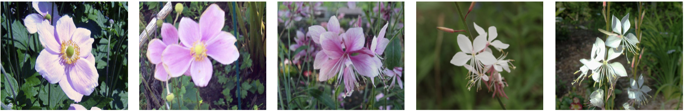
(a) Oxford 102 Flowers image samples.

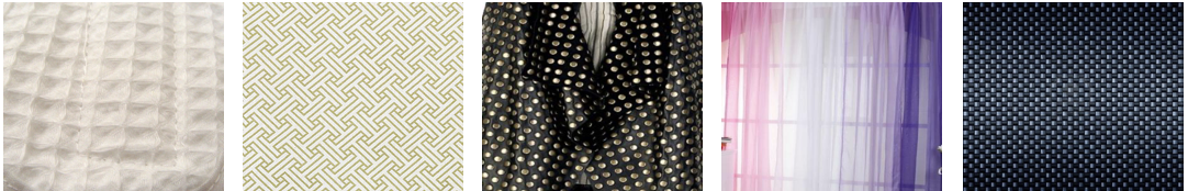
(b) DTD image samples.

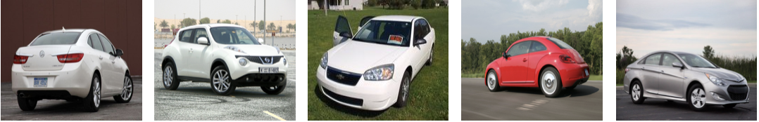
(c) Stanford Cars image samples.

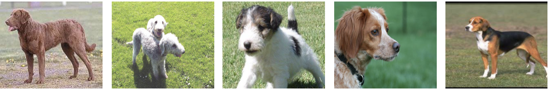
(d) Stanford Dogs image samples.

Figure 7: Besides FGVC-Aircraft shown in Figure 5, (a) Oxford 102 Flowers, (b) DTD, (c) Stanford Cars, and (d) Stanford Dogs are used for domain adaptation experiments. They are fine-grained datasets consisting of a small number of images. Fine-grained classification datasets are composed of limited categories with barely discernible details which make them difficult to be distinguished. It is even more challenging for DNN to learn enough knowledge of those domains by a small number of images.

References

- [1] Karen Simonyan and Andrew Zisserman. Very deep convolutional networks for large-scale image recognition. arXiv preprint arXiv:1409.1556, 2014.
- [2] Qianru Sun, Yaoyao Liu, Tat-Seng Chua, and Bernt Schiele. Meta-transfer learning for few-shot learning. In Proceedings of the IEEE/CVF Conference on Computaer Vision and Pattern Recognition, pages 403–412, 2019.
- [3] Alexander Kolesnikov, Alexey Dosovitskiy, Dirk Weissenborn, Georg Heigold, Jakob Uszkoreit, Lucas Beyer, Matthias Minderer, Mostafa Dehghani, Neil Houlsby, Sylvain Gelly, et al. An image is worth 16x16 words: Transformers for image recognition at scale. 2021.
- [4] Aditya Ramesh, Mikhail Pavlov, Gabriel Goh, Scott Gray, Chelsea Voss, Alec Radford, Mark Chen, and Ilya Sutskever. Zero-shot text-to-image generation, 2021.
- [5] Tomáš Chobola, Daniel Vašata, and Pavel Kordík. Transfer learning based few-shot classification using optimal transport mapping from preprocessed latent space of backbone neural network. arXiv preprint arXiv:2102.05176, 2021.
- [6] Jakub Konečnỳ, H Brendan McMahan, Felix X Yu, Peter Richtárik, Ananda Theertha Suresh, and Dave Bacon. Federated learning: Strategies for improving communication efficiency. arXiv preprint arXiv:1610.05492, 2016.
- [7] Wei Yang Bryan Lim, Nguyen Cong Luong, Dinh Thai Hoang, Yutao Jiao, Ying-Chang Liang, Qiang Yang, Dusit Niyato, and Chunyan Miao. Federated learning in mobile edge networks: A comprehensive survey. IEEE Communications Surveys & Tutorials, 22(3):2031–2063, 2020.
- [8] Andrew G Howard, Menglong Zhu, Bo Chen, Dmitry Kalenichenko, Weijun Wang, Tobias Weyand, Marco Andreetto, and Hartwig Adam. Mobilenets: Efficient convolutional neural networks for mobile vision applications. arXiv preprint arXiv:1704.04861, 2017.
- [9] Mark Sandler, Andrew Howard, Menglong Zhu, Andrey Zhmoginov, and Liang-Chieh Chen. Mobilenetv2: Inverted residuals and linear bottlenecks. In Proceedings of the IEEE conference on computer vision and pattern recognition, pages 4510–4520, 2018.
- [10] Xiangyu Zhang, Xinyu Zhou, Mengxiao Lin, and Jian Sun. Shufflenet: An extremely efficient convolutional neural network for mobile devices. In Proceedings of the IEEE conference on computer vision and pattern recognition, pages 6848–6856, 2018.
- [11] Ningning Ma, Xiangyu Zhang, Hai-Tao Zheng, and Jian Sun. Shufflenet v2: Practical guidelines for efficient cnn architecture design. In Proceedings of the European conference on computer vision (ECCV), pages 116–131, 2018.
- [12] Mingxing Tan and Quoc Le. Efficientnet: Rethinking model scaling for convolutional neural networks. In International Conference on Machine Learning, pages 6105–6114. PMLR, 2019.
- [13] Mingxing Tan and Quoc V Le. Efficientnetv2: Smaller models and faster training. arXiv preprint arXiv:2104.00298, 2021.
- [14] Pramod Kaushik Mudrakarta, Mark Sandler, Andrey Zhmoginov, and Andrew Howard. K for the price of 1: Parameter-efficient multi-task and transfer learning. arXiv preprint arXiv:1810.10703, 2018.
- [15] Sylvestre-Alvise Rebuffi, Hakan Bilen, and Andrea Vedaldi. Learning multiple visual domains with residual adapters. arXiv preprint arXiv:1705.08045, 2017.
- [16] Sylvestre-Alvise Rebuffi, Hakan Bilen, and Andrea Vedaldi. Efficient parametrization of multi-domain deep neural networks. In Proceedings of the IEEE Conference on Computer Vision and Pattern Recognition, pages 8119–8127, 2018.
- [17] Rodrigo Berriel, Stephane Lathuillere, Moin Nabi, Tassilo Klein, Thiago Oliveira-Santos, Nicu Sebe, and Elisa Ricci. Budget-aware adapters for multi-domain learning. In Proceedings of the IEEE/CVF International Conference on Computer Vision, pages 382–391, 2019.
- [18] Eleni Triantafillou, Hugo Larochelle, Richard Zemel, and Vincent Dumoulin. Learning a universal template for few-shot dataset generalization. arXiv preprint arXiv:2105.07029, 2021.
- [19] Han Cai, Chuang Gan, Ligeng Zhu, and Song Han. Tinytl: Reduce memory, not parameters for efficient on-device learning. arXiv preprint arXiv:2007.11622, 2020.
- [20] Debesh Jha, Anis Yazidi, Michael A Riegler, Dag Johansen, Håvard D Johansen, and Pål Halvorsen. Lightlayers: Parameter efficient dense and convolutional layers for image classification. In International Conference on Parallel and Distributed Computing: Applications and Technologies, pages 285–296. Springer, 2020.
- [21] Yeming Wen, Dustin Tran, and Jimmy Ba. Batchensemble: an alternative approach to efficient ensemble and lifelong learning. arXiv preprint arXiv:2002.06715, 2020.
- [22] Abolfazl Farahani, Sahar Voghoei, Khaled Rasheed, and Hamid R Arabnia. A brief review of domain adaptation. Advances in Data Science and Information Engineering, pages 877–894, 2021.
- [23] Olga Russakovsky, Jia Deng, Hao Su, Jonathan Krause, Sanjeev Satheesh, Sean Ma, Zhiheng Huang, Andrej Karpathy, Aditya Khosla, Michael Bernstein, et al. Imagenet large scale visual recognition challenge. International journal of computer vision, 115(3):211–252, 2015.
- [24] Subhransu Maji, Esa Rahtu, Juho Kannala, Matthew Blaschko, and Andrea Vedaldi. Fine-grained visual classification of aircraft. arXiv preprint arXiv:1306.5151, 2013.
- [25] Jonathan Krause, Michael Stark, Jia Deng, and Li Fei-Fei. 3d object representations for fine-grained categorization. In Proceedings of the IEEE international conference on computer vision workshops, pages 554–561, 2013.
- [26] Mircea Cimpoi, Subhransu Maji, Iasonas Kokkinos, Sammy Mohamed, and Andrea Vedaldi. Describing textures in the wild. In Proceedings of the IEEE Conference on Computer Vision and Pattern Recognition, pages 3606–3613, 2014.
- [27] Maria-Elena Nilsback and Andrew Zisserman. Automated flower classification over a large number of classes. In 2008 Sixth Indian Conference on Computer Vision, Graphics & Image Processing, pages 722–729. IEEE, 2008.
- [28] Aditya Khosla, Nityananda Jayadevaprakash, Bangpeng Yao, and Fei-Fei Li. Novel dataset for fine-grained image categorization: Stanford dogs. In Proc. CVPR Workshop on Fine-Grained Visual Categorization (FGVC), volume 2. Citeseer, 2011.