Perturbation Analysis of Randomized SVD and its Applications to High-dimensional Statistics
Supplementary File for “Perturbation Analysis of Randomized SVD and its Applications to High-dimensional Statistics”
Abstract
Randomized singular value decomposition (RSVD) is a class of computationally efficient algorithms for computing the truncated SVD of large data matrices. Given an symmetric matrix , the prototypical RSVD algorithm outputs an approximation of the leading singular vectors of by computing the SVD of ; here is an integer and is a random Gaussian sketching matrix. In this paper we study the statistical properties of RSVD under a general “signal-plus-noise” framework, i.e., the observed matrix is assumed to be an additive perturbation of some true but unknown signal matrix . We first derive upper bounds for the and distances between the approximate singular vectors of and the true singular vectors of . These upper bounds depend on the signal-to-noise ratio (SNR) and the number of power iterations . A phase transition phenomenon is observed in which a smaller SNR requires larger values of to guarantee convergence of the and distances. We also show that the thresholds for where these phase transitions occur are sharp whenever the noise matrices satisfy a certain trace growth condition. Finally, we derive normal approximations for the row-wise fluctuations of these approximate singular vectors and the entrywise fluctuations when is projected onto these vectors. We illustrate our theoretical results by deriving nearly-optimal performance guarantees for RSVD when applied to three statistical inference problems, namely, community detection, matrix completion, and PCA with missing data.
Abstract
The Supplementary File can be divided to four parts. Section S.1 presents several numerical experiments to verify our main theoretical investigations. Section S.2 contains an extension of our main results to the case of asymmetric and . Section S.3 states more general counterparts of our main theorems when is assumed to be non-random. Sections S.4–S.7 include all the technical lemmas and proofs.
and
1 Introduction
Spectral methods are popular in statistics and machine learning as they provide computationally efficient algorithms with strong theoretical guarantees for a diverse number of inference problems including network analysis [91, 99, 113], matrix completion and denoising [4, 23], covariance estimation/PCA [66, 50], non-linear dimension reduction and manifold learning [114, 12, 32], ranking [26, 27], etc. A common unifying theme for many spectral algorithms is, given a data matrix , first compute a factorization of using the ubiquitous singular value decomposition (SVD), then truncate this SVD to keep only the leading singular values and singular vectors, and finally perform inference using the truncated SVD representation. The value is usually chosen to be as small as possible while still preserving most of the information in .
Classical algorithms for SVD, such as those based on pivotal QR decompositions and/or Householder transformations, require floating-point operations (flops) assuming and return the full set of singular values and vectors, even when only the leading of them are desired; see Sections 5.4 and 8.3 of [55]. The flops is a severe computational burden when is large. These algorithms also require random access to the entries of and are thus inefficient when is too large to store in RAM. These computation and memory issues limit the use of classical SVD in modern data applications.
Recently in the numerical linear algebra community, randomized SVD (RSVD) [101, 58, 116, 89, 117] had been widely studied with the aim of providing fast, memory efficient, and accurate approximations for the truncated SVD of large data matrices. In particular, suppose is an matrix and we are interested in finding the leading (left) singular vectors of for some . The prototypical RSVD algorithm [58] first sketches into a smaller matrix where and are user-specified parameters and is a random matrix, and then uses the leading left singular vectors of as an approximation to the leading left singular vectors of . The parameter is usually chosen to be a small integer and is chosen to be equal to or slightly larger than . There are numerous choices for including Gaussian matrices, random orthogonal matrices, Rademacher matrices, and column-subsampling matrices; see [83, 124, 68] and the references therein.
The sketch-and-solve strategy of RSVD has several important practical advantages. Firstly, it has a computational complexity of flops and this can be further reduced to flops when the sketching matrix is structured. These or flops are also very fast as the main operations are the matrix-matrix products and where is either a or matrix; matrix products are highly-optimized on almost all computing platforms. Secondly, it is “pass efficient” [41, 58] and only requires passes through the data; this dramatically reduces memory storage [55, 81]. Thirdly, RSVD also allows for data compression [33] and can be adapted to a streaming setting [116]. Many recent works have discussed replacing the classical SVD with RSVD, see [118, 36, 97, 62, 78, 49, 9, 95] for examples in covariance matrix estimation, matrix completion, network embeddings, and dynamic mode decompositions.
Existing theoretical results for RSVD, such as those in [101, 58, 59, 106, 81], had mainly focused on the setting where is assumed to be noise-free; these results either bound the approximation error between and or bound the difference between the low-rank approximation error of and that of . Here denote the true leading singular vectors of and denote some unitarily invariant norm. In particular these approximation error decreases if (the number of power iterations) and/or (the sketching dimensions) increases. However, for many inference problem, the observed matrix is also noisy due to sampling and/or perturbation errors. More specifically it is often the case that is generated from a “signal-plus-noise” model where is assumed to be the underlying true signal matrix of with certain structure e.g., (approximately) low rank and/or sparse, and is the unobservable perturbation noise. As is a noisy realization of , is a noisy estimate of , the leading singular vectors of . Under this perspective, the main aim is now to understand the relationship between and , and we thus need to balance between the approximation error of and the estimation error of , i.e., it is neither necessary nor beneficial to make the approximation error between and much smaller than the estimation error between and .
Estimation errors between and is a fundamental topic in matrix perturbation theory. Classic results in matrix perturbation include Weyl’s and Lidskii’s inequalities [123, 80] for eigenvalues and singular values, and the Davis–Kahan Theorem and Wedin’s Theorem [38, 129, 122] for subspaces; these results make minimal assumptions on the perturbation matrices . The last decade has witnessed further study of matrix perturbations from more statistical perspectives through the introduction of additional minor assumptions on and such as the entries of are independent random variables and/or the leading singular vectors of has bounded coherence. Examples include more refined matrix concentration inequalities [115, 104, 93, 5], rate-optimal unilateral singular subspace perturbation bound [17], and singular subspace perturbation bounds [3, 51, 46, 84, 21, 22, 75]. These developments in turns lead to stronger statistical guarantees for many spectral methods; see [28] for a recent and comprehensive survey.
In this paper, we will study the perturbation error between and under the ”signal-plus-noise” model described above. In particular we analyze a repeated sampling version of RSVD (namely, rs-RSVD) with complexity where is the number of random sketches and is the number of power iterations of ; see Section 2. The choice corresponds to the PowerRangeFinder and SubspacePowerMethod described in [58, 124, 89]. Theoretical results for rs-RSVD, under a set of mild and typically seen assumptions for , are presented in Section 3. These results include perturbation bounds for the difference in either or norm between the approximate singular vectors of and the true singular vectors of , normal approximations for the row-wise fluctuations of , and entrywise concentration and normal approximations for . The and bounds exhibit a phase-transition phenomenon in that as the signal-to-noise ratio (SNR) decreases, the number of power iterations need to increase to guarantee fast convergence rates; the phase transition thresholds are also sharp provided that the noise matrices satisfy a certain trace growth conditions. We then apply our theoretical results to three different statistical inference problems: community detection, matrix completion, and PCA with missing data. For all three problems we show that the approximate singular vectors achieve the same or nearly the same theoretical guarantees as that for the true singular vectors ; see Section 4 and Section 5. Our results thus provide a bridge between the numerical linear algebra and statistics communities. For conciseness and ease of exposition we only present results for symmetric and in the main paper. Extension of these results to the case of asymmetric and are provided in Section S.2 of the supplementary document. Numerical experiments and detailed proofs for the main paper are also included in the supplementary document.
2 Background and settings
2.1 Notation
Let be a positive integer. We then write to denote the set . For two sequences and , we write if there exists a constant not depending on such that for all but finitely many ; we write if and we write if and .
The set of matrices with orthonormal columns is denoted as when and is denoted as otherwise. Let and be symmetric matrices. We write if is positive semidefinite and we write if is positive definite. Let be an arbitrary matrix. We denote the th row of by , and the th entry of by . We write and to denote the trace and rank of a square matrix , respectively. The spectral and Frobenius norm of are denoted as and , respectively. The maximum (in modulus) of the entries of is denoted as . In addition we denote the norm of by
i.e., is the maximum of the norms of the rows of . We have the relationships
where and are the number of rows and columns of , respectively. Given two matrices and , we define their and distances as
Recall that where are the principal angles between and . Furthermore, by the relationship between the spectral and norms, yields finer and more uniform control of the row-wise differences (up to orthogonal transformations) between and . See [22, 75, 34, 3, 28] for further discussions of the and its uses in matrix perturbation inequalities and statistics applications.
2.2 Signal-plus-noise perturbation framework
For ease of exposition we restrict ourselves to the case when the observed matrices are symmetric in the main paper. The general case of rectangular and/or asymmetric matrices are presented in Section S.2 of the supplementary document. For a symmetric matrix with , we consider the additive perturbation
where is a symmetric noise matrix; we shall generally assume that and are unobserved, i.e., we observed only . Denote the eigendecompositions of and by
| (2.1) | ||||
where and are diagonal matrices containing the largest (in magnitude) nonzero eigenvalues of and , respectively. Let denote the condition number for the first eigenvalues of .
We focus mainly on the setting where has an approximately low-rank structure, i.e., both and are either bounded or slowly diverging; we say that a quantity depending on is slowly diverging if as . These low-rank assumptions appear frequently in many inference problems for high-dimensional matrix-valued data including community detection in graphs, matrix completion, and covariance matrix estimation; see e.g., [46, 3, 51, 21, 88, 16] among others. We now make an assumption on .
Assumption 1 (Signal-to-Noise Ratio).
Let . There exists fixed but arbitrary constants and a quantity depending on such that and
| (2.2) |
whenever . We view as the noise level of and as a lower bound on the SNR.
Assumption 1 provides a concentration inequality for in terms of and the signal to noise ratio (SNR) . As , Assumption 1 guarantees that and hence, by Weyl’s inequality, there exists with high probability a sufficiently large gap between the leading eigenvalues of (as induced by the signal ) and the remaining eigenvalues of (as induced by the noise ). This allows us to relate the singular vectors of the sketched matrix to the leading singular vectors of as increases. We show in Section 3 that, as the SNR decreases, we need larger values of to accurately recover the singular subspace of from that of .
We emphasize that Assumption 1 generally holds if is a symmetric matrix whose upper triangular entries are independent mean random variables. Examples include the case where the entries of are either Gaussian random variables with variances bounded by or bounded random variables with variances bounded by ; see e.g., Corollary 3.9 in [11] or Theorem 1.4 in [115] for a justification of these claims. Furthermore the lower bound in Eq. (2.2) is somewhat arbitrary and is chosen mainly for convenience. Indeed, the above cited results also show that for any constant there exists a constant depending only on such that with probability at least . This constant can then be subsumed into the definition of without changing the SNR . Assumption 1 can also hold when the entries of are not mutually independent. See for example the presentation of PCA with missing data in Section 5.2, i.e., the matrix in Section 5.2 is is of the form where is a deterministic symmetric matrix and is a matrix whose entries are independent random variables. The product creates dependence between the upper triangular entries of .
Finally we note that the noise level in Assumption 1 is possibly decoupled from the signal strength . This is intentional as it allows us to obtain more general theoretical results that can then be applied in diverse settings. For example in Section 4 we consider the random graphs setting wherein the entries of are binary random variables with . The distribution of therefore depends only on and thus is also a function of . In particular and so as the signal level decreases (for example either by decreasing the number of non-zero entries and/or their magnitudes) the SNR also decreases and inference using becomes harder. In contrast, for the problems of matrix completion and PCA with missing data discussed in Section 5, the distribution for depends on other parameters distinct from and it is thus possible to reduce both and without changing the SNR, thereby not affecting the general behavior of .
2.3 Randomized SVD with repeated sampling
Given we wish to find the eigenvectors associated with the largest eigenvalues (in magnitude) of . One popular and widely used approach for finding is via randomized subspace iteration. More specifically we first sample an matrix whose entries are iid standard normals and compute for some positive integer . Now let be the matrix whose columns form an orthonormal basis for the leading left singular vectors of . The matrix is a low rank approximation to and we can take as an approximation to . We note that , the number of columns of , is often chosen to be slightly larger than in order to increase the probability that the column space of also include the column space of ; empirical observations suggest that or is sufficient for most practical applications [58, Section 1.3]. For more discussion on randomized subspace iteration, see Section 4.5 of [58], Section 11.6 of [86], Section 4.3 of [124], and [89]. Recently, [81] has purposed a data-driven bootstrap algorithm to estimate the approximation error of sketching SVD, which might also be adapted to select for the general RSVD in practice.
This paper considers a variant of the above procedure in which we sample independent realizations and choose the which maximizes ; here denotes the th largest singular value of a matrix. We term the resulting procedure as repeated-sampling randomized SVD (rs-RSVD); see Algorithm 1 for a formal description. The main rationale for the repeated sampling step is that letting allows us to choose , which results in having the smallest number of columns while still obtaining an estimate of that is qualitatively similar to that when ; see the theoretical results in Section 3 and the numerical experiments in Sections S.1 in the Supplementary File for demonstrations of this claim. In addition, if arises from the additive model described in Section 2.2 then also leads to simpler theoretical results compared to .
Remark 2.1 (Implementation details for Algorithm 1).
For ease of exposition we had written steps 1–3 of Algorithm 1 as if there were different sketches . As the computation of involves passes through the data matrix , having is undesirable if we then require passes, especially when the dimensions of are large. In practice we can combine all different sketches into a single sketch, i.e., as the are iid, we first generate a standard Gaussian matrix with rows and columns, compute a single sketched matrix , and then form the by sequentially extracting (without replacement) columns from . The number of passes through the data is then still . We can also replace Algorithm 1 with a more numerically stable albeit algebraically equivalent version wherein one periodically orthonormalizes (using QR decomposition) for before computing ; see [58, Remark 4.3] and [85]. This extra orthonormalization step has no impact on the theoretical results presented subsequently.
Remark 2.2 (Sketching with ).
If we set both and in Algorithm 1 then we get the “sketched SVD” algorithm described in [81, 83]. Sketched SVD is very useful when is too large to store in fast memory as the procedure only requires one pass through the data. However, as we will show in Section 4, setting leads to poor estimates of using rs-RSVD unless ; indeed the theoretical analysis in this paper can be extended to show that if then is possibly necessary to guarantee accurate estimation of using rs-RSVD; the choice has recently been considered by [126],which helps to establish precise asymptotically exact results in the context of sketching PCA. In practice, it is usually preferable to choose as small as possible, thus we will not present theoretical results for the regime as it detracts from the main message of current paper.
3 Theoretical results
We now present large-sample deviation and fluctuation results between the approximate singular vectors of (as obtained via rs-RSVD) and the true singular vectors of the signal matrix . In particular Sections 3.1 and 3.2 give high-probability and perturbation bounds (deviations) of . The normal approximation for the row-wise fluctuations of is given in Section 3.4.
We first introduce some notation. Let the SVDs of and be denoted as
| (3.1) | ||||
where and contain the largest singular values of and , respectively. Recall that we assumed . The following proposition shows that the leading singular vectors of and are equivalent.
Proposition 3.1.
Let be a Gaussian random matrix with . Let be a finite positive integer. Then almost surely.
Proposition 3.1 requires the sketching dimension to be no smaller than , the rank of , but allows for to be any positive integer. This requirement also indicates that the sketching of is generally more difficult compared to that of , even when with high probability. Indeed, is usually full-rank and hence the leading singular vectors of need not be close to that of for any arbitrary .
Remark 3.1.
(Known ) In this paper we focus on the scenario where the parameter in Algorithm 1 is correctly specified, i.e., , and thus is used interchangeably with in the following theoretical results. In practice might be unknown and need to be estimated. There are a large number of methods for estimating consistently and a few representative, but by no means exhaustive, references include [94, 132, 6, 60, 127]. We note, however, that all of the approaches described in these references require knowing the leading singular values of and this is possibly problematic in the context of RSVD if these singular values have to be first computed using some classical SVD algorithm. Estimation of can also be done within -RSVD itself using similar ideas to that in Sections 4.3 and 4.4 of [58] and while we surmise that the consistency of the these estimates are reasonably straightforward to establish, they nevertheless involve additional notations and derivations. We thus decided to leave the simultaneous estimation of and using RSVD for future work.
Remark 3.2 (Distribution for ).
In addition to standard Gaussian, other distributions for such as uniform and Rademacher distributions have also been studied [83, 124, 68]. We focus on the Gaussian distribution mainly for ease of exposition; any distribution for which satisfies Proposition 3.1 and Lemmas S.4.4–S.4.5 in the Supplementary File, will also lead to the same theoretical results as that presented in Theorems 3.1–3.3 of this paper. In particular if is such that then Proposition 3.1 holds. If has iid sub-Gaussian entries then Lemmas S.4.4–S.4.5 also hold (using existing results on the smallest singular values of random matrices from [105]). Thus the main theorems of this paper remain unchanged if the entries of are uniformly distributed. The case where is Rademacher requires further analysis as and Proposition 3.1 no longer holds.
3.1 error bound
Proposition 3.1 implies the almost-sure equivalence between and . Thus, to obtain a perturbation bound between and , we can alternatively study the perturbation between and ; Recall that and are the left singular matrices of and . We first derive an upper bound for using the expansion for introduced in Lemma S.4.2; see Theorem S.3.1. This upper bound depends on the SNR as well as several quantities that depend only on the sketching matrix . We bound the quantities depending on separately (see Lemma S.4.4 and Lemma S.4.5) and thereby obtain the following result.
Theorem 3.1.
By Wedin’s Theorem [122], the spectral-norm concentration in Theorem 3.1 together with the lower bound for in Lemma S.4.5 yield the following bound for .
Theorem 3.2.
Suppose Assumption 1 hold, and that is generated via Algorithm 1 for some satisfying either one of the following three conditions:
-
(a)
both and are fixed.
-
(b)
is fixed and is growing with .
-
(c)
is growing with and for any fixed .
Assume the condition number satisfies . Choose where is a constant not depending on . Then for any we have, with probability at least ,
| (3.4) |
Recall is defined in Theorem 3.1.
Remark 3.3.
Theorem 3.2 also yields a perturbation bound between the (approximate) singular values obtained from Algorithm 1 and the true singular values of .
Corollary 3.1.
Assumption 1 together with Weyl’s inequality implies that with high probability where are the (exact) leading singular values of . Corollary 3.1 thus indicates that the estimation error rate of is the same as that for , up to some factors depending on the conditional number and ; recall that when and is either bounded or, at most, slowly-diverging.
3.2 norm error bound
We now study the perturbation between and . As the norm is generally more stringent than the norm, we introduce an additional assumption on the row-wise fluctuations of for .
Assumption 2.
There exist positive constants and such that, for any , any positive integer , any standard basis , and any vector not dependent on , we have with probability at least that
| (3.6) |
Here is the th basis vector in and is a finite constant depending possibly on but not on and .
The concentration bound in Eq. (3.6) appears frequently in the literature on perturbation, see e.g., [100, 90, 46, 35, 21, 84], and is satisfied by a large class of random matrices . More specifically, Proposition 3.2 below shows that if is a (generalized) Wigner matrix whose entries are independent mean random variables with subexponential tails then satisfies Assumption 2. Proposition 3.2 is motivated by Remark 2.5 in [48] and we will use it to verify Assumption 2 for the noise matrices considered in Sections 4 and 5. We also note that the probability lower bound of Eq. (3.6) is somewhat arbitrary and is chosen mainly for convenience. Indeed, Proposition 3.2 shows that for any there exists a depending on such that the left hand side of Eq. (3.6) holds with probability at least whenever . See also the discussion after Assumption 1.
Proposition 3.2.
Let be a matrix whose entries (or upper triangular entries if is symmetric) are independent zero-mean random variables. Suppose that there exist a constant not depending on and a quantity such that
for all , and integer ; here is a fixed constant, is the quantity appearing in Assumption 1, and as . Then for any fixed constant , any integer , and any vector not dependent on , we have
with probability at least , provided that . Here and are constants depending only on , and the divergence rate of .
We now provide two simple examples illustrating the use of Proposition 3.2.
Example 1 (Bernoulli Entries).
Let be a finite constant not depending on . Let be a symmetric matrix with independent upper triangular entries such that, for all we have with probability and with probability , for some . Suppose furthermore that satisfies as . This type of matrix appears frequently in random graph inference; see Section 4. Now let . If then Eq. (3.6) follows from Bernstein’s inequality with (see e.g. Lemma 16 in [3]). Now suppose that and let . Then, after some straightforward algebra, we have (1) and (2) there exist some such that for all ,
where the first inequality is because for all . The matrix satisfies the conditions in Proposition 3.2 and hence satisfies Assumption 2.
Example 2 (Sub-Gaussian Entries).
Let be symmetric with independent zero-mean sub-Gaussian entries whose Orlicz-2 norms are bounded from above by . Let . If then Eq. (3.6) follows from a general version of Hoeffding’s inequality (see e.g., Theorem 2.6.3 in [120]) with . Now suppose . We then have [120, § 2.5.2] which implies the moment condition
Let , , and , we have
We have thus verified all conditions in Proposition 3.2 hence satisfies Assumption 2.
Given Assumption 2, the derivation of our bounds proceeds as follows. We first combine the Procrustean matrix decomposition in Theorem 3.1 of [22] with the series expansion for given in Lemma S.4.2. This yields an expression for that depends mainly on two type of terms, namely (1) terms of the form for some matrix of dimensions or where does not depend on , and (2) terms of the form for some not depending on . The terms are bounded using the concentration inequality in Assumption 2 while the terms are bounded in a similar manner to those in Theorem 3.2; see Theorem S.3.3 and Lemma S.4.4 to Lemma S.4.6 in the Supplementary File, for more details. In summary we obtain the following result.
Theorem 3.3.
The upper bound in Eq. (3.7) decreases with . Furthermore, as , we have always. The quantity is termed the coherence of [20]. A matrix with is said to have bounded coherence; bounded coherence for is a prevalent and typically mild assumption in many high-dimensional statistics problem including matrix completion, covariance estimation, subspace estimation, and random graph inference; see e.g., [20, 51, 75, 3, 22, 18] and the examples in Section 4 and Section 5 of this paper.
Remark 3.4.
The upper bound in Eq. (3.7) requires and is slightly sharper when ; indeed if while if and . This difference is, however, very minor. Indeed, as is an integer, is possible only when for integers . If then a similar bound to Eq. (3.7) is available, albeit with a provably worse upper bound, i.e., with probability at least ,
| (3.8) |
where and are defined in Eq. (S.5.27) and Eq. (S.5.28) of the supplementary.
Remark 3.5.
For ease of exposition we have stated Eq. (3.6) in terms of a single for all . We can instead assume that there exists a non-decreasing and bounded sequence such that, for all we have
with probability at least . Then Theorem 3.3 still holds under the above assumption but with and this allows for a more precise control of the factor in Eq. (3.7). Indeed, as we see from Example 1 and Example 2 above, for many inference problem such as network analysis and matrix completion we can control using either Bernstein’s inequality or Hoeffding’s inequality so that ; the remaining are bounded from above by some finite constant via Proposition 3.2. With the term in Theorem 3.3 (and Corollary 3.2 later) is simplified to when and ; this factor is generally optimal.
Remark 3.6.
Bounds for can be derived using several different approaches, including leave-one-out analysis [3, 27, 18, 3], von Neumann series expansion [46, 24, 30], holomorphic functional analysis [75], and techniques tailored towards Gaussian ensembles [73, 72, 71]. See [28] for a comprehensive survey. Our work, meanwhile, focuses on . As is obtained from the SVD of , the bounds for depends on which has a substantially more complicated entrywise dependency structure than that in . As a result not all of the above cited techniques are directly applicable for bounding . For this paper we combine the Procrustean analysis argument from [22] with the expansion for given in Lemma S.4.2. This approach yields a perturbation expansion for that includes auxiliary terms of the form where does not depend on , and we leveraged Assumption 2 and Proposition 3.2 to bound these terms. We leave the problem of adapting other techniques (such as leave-one-out analysis) to control the row-wise deviation of for future work.
The row-wise fluctuation for in Theorem 3.3 also yields an entrywise concentration bound for . In particular we have the following result.
Corollary 3.2.
Assume the setting of Theorem 3.3 and suppose that both and are bounded as increases. Let . We then have
with probability at least ; here satisfies if and otherwise.
3.3 Comparison with existing results
We now compare the perturbation bounds for in and norms with existing results in the literature. As we mentioned in the introduction, most theoretical analysis of RSVD focused exclusively on the setting where is assumed to be noise-free and the quantities of interest are bounds for in either spectral norm or Frobenius norm. For example by combining Theorem 9.2 and Theorem 10.8 in [58] we have that if is symmetric and then
| (3.9) |
with high probability. Here and denote the th largest singular value of . If where and satisfy Assumption 1 then, without additional information, we can only conclude that . Eq. (3.9) then reduces to
with high probability, for any fixed . Recall that is a low rank approximation of and serves as an estimate of the true but unknown signal matrix . Invoking Assumption 1 again we obtain
| (3.10) |
with high probability. On the other hand, Theorem 3.2 of this paper implies
| (3.11) |
with high probability. Note that Eq. (3.11) is much sharper than Eq. (3.10) when is (approximately) low-rank as assumed in the current paper. Indeed if is bounded or slowly diverging then the multiplicative factor in Eq. (3.11) is either bounded or of order for any arbitrary constant while the multiplicative factor in Eq. (3.10) is and thus requires to be competitive with the bound in Eq. (3.11); note that power iterations was also used in the theoretical analysis of RSVD in [89] and Theorem 60 in [124]; as we only require , our bounds are more closely tailored to the setting of noisy . Finally note that with high probability. Thus attains the same error rate as , up to some (at most) logarithmic factor.
The above bounds for are based on . We now consider the implication of the bounds for . Suppose has bounded coherence, i.e., , and satisfies Assumption 2. Let and are as specified in Theorem 3.3. If and are slowly growing then Corollary 3.2 implies
| (3.12) |
with high probability. Eq. (3.12) is, to the best of our knowledge, the first bound for entrywise differences between the RSVD-based low-rank approximation of the noisily observed and the underlying signal matrix , and provides much finer control for . Eq. (3.12) cannot be obtained by simply combining existing bounds for (as given in the RSVD literature) and bounds for (as given in the matrix perturbation literature); here denote any unitarily invariant norm. Finally, as we will see in Sections 5.1, the bound in Eq. (3.12) can have the same error rate as that for , up to some (at most) logarithmic factor.
3.4 Row-wise limiting distribution
The row-wise limiting distribution of singular vectors can be applied for uncertainty quantification of membership inference in network analysis [77, 10]. Under some appropriate probabilistic structures of and , is proved to have a row-wise limiting distribution [21]. In this section we prove that also has row-wise asymptotic normal distributions, provided that and satisfy the following condition.
Assumption 3.
Let be a sequence of bounded non-negative numbers which can converge to as . Assume that both of the following conditions hold as .
-
(a).
satisfies Assumption 1 with and for some constant .
-
(b).
For any fixed , we have
(3.13) where is a deterministic matrix depending possibly on and .
Assumption 3 is valid for more general and , compared with Assumption 5 in [21], which typically focuses on a random graph context. One scenario for which Assumption 3 holds is when has symmetrically independent entries and the variances of entries in are of the same asymptotic order , while the variance of the other entries are negligible. Such entrywise independent and homogenous conditions of appear frequently in many statistical problems including matrix completion, graph embeddings, and multi-dimensional scaling; see e.g., [21, 79, 23].
Theorem 3.4.
Suppose Assumptions 1–3 hold with fixed and bounded . Let be generated via Algorithm 1 with , where the universal constant is given in Remark 3.3, and . Now suppose that as , we have
| (3.14) |
in probability, where is a logarithmic factor such that
| (3.15) |
Then there exist a sequence of orthogonal matrices such that for any ,
For each the matrix solves the orthogonal Procrustes problem between and (see Eq. (S.5.47)).
The condition in Theorem 3.4 is slightly more stringent than the condition in Theorem 3.1 and Theorem 3.3. The main reason for this discrepancy is that while might be sufficient for and to achieve the optimal error rate, it does not guarantee that the row-wise fluctuations of is asymptotically equivalent to the row-wise fluctuations of given in Assumption 3. We will present, in Section S.1.1.3 in the Supplementary File, simulation results for the row-wise Gaussian fluctuations of when is the adjacency matrix of a SBM random graph; our simulations indicate that the condition is in fact necessary and sufficient.
Remark 3.7.
We now make a few technical remarks concerning Theorem 3.4.
-
1.
Theorem 3.4 can be extended to the case where either (or both) of and are slowly diverging, provided that we also increase the exponent for in the definition of .
-
2.
The term in Eq. (3.14) can usually be bounded by with high probability. More specifically, let be a symmetric matrix whose upper triangular entries are independent mean random variables with and for all . Now if then, by Bernstein inequality,
with high probability; see Eq. (4.137) in [28] for more details. Thus converges to in probability whenever . Recall that .
-
3.
The term in Eq. (3.14) depends on the SNR and the coherence of i.e., this term is equivalent to . Thus larger values of require larger SNR in order to guarantee convergence in Eq. (3.14). If has bounded coherence, i.e., is bounded, then due to our assumption that . As we alluded to earlier, bounded coherence for is a prevalent and typically mild assumption in many high-dimensional statistics problem including matrix completion, covariance estimation, subspace estimation, and random graph inference; see e.g., [20, 51, 75, 3, 22, 18].
- 4.
4 Random graph inference
As an illustrative example of Theorem 3.2 and Theorem 3.3, we consider the problem of estimating the leading eigenvectors for edge-independent random graphs with low-rank edge probabilities matrices. More specifically, let be the adjacency matrix of a random graph on vertices with edge probabilities i.e., is a symmetric, binary matrix whose upper triangular entries are independent Bernoulli random variables with . Next assume that is of rank for some fixed and has bounded condition number, i.e., for some fixed constant . Let and suppose that Assumption 1 holds with
| (4.1) |
for some fixed constant . We interpret as the average expected degree for the vertices of , i.e., with high probability has non-zero entries. Smaller values of thus implies sparser networks. We note that Eq. (4.1) is satisfied by many random graph models including Erdős–Rényi [47], SBM and its degree-corrected and/or mixed-membership variants [63, 69, 108, 7], (generalized) random dot product graphs [128, 103], as well as any edge-independent random graph whose edge probabilities are sufficiently homogeneous, e.g., for all . Assumption 2 is also satisfied by the random graphs mentioned above; see e.g. [48, 21, 84] and Example 1. In addition, we also assume the bounded coherence for , This is a prevalent and typically mild assumption for random graphs, see e.g., [75, 3, 22].
4.1 Subspace perturbation error bound
Now consider the case where , the number of vertices in , is large and the graph is possibly semi-sparse, and we are interested in computing the leading singular vectors of as an estimate for the leading singular vectors of . To save computational time, we will use Algorithm 1 to approximate the singular vectors of . Now suppose we choose a fixed , and either and or and ; recall that is the sketching dimension and is the number of repeated sampling steps. Then from Theorems 3.2 and 3.3 (and the corresponding remarks) we have that, with high probability,
| (4.2) | ||||
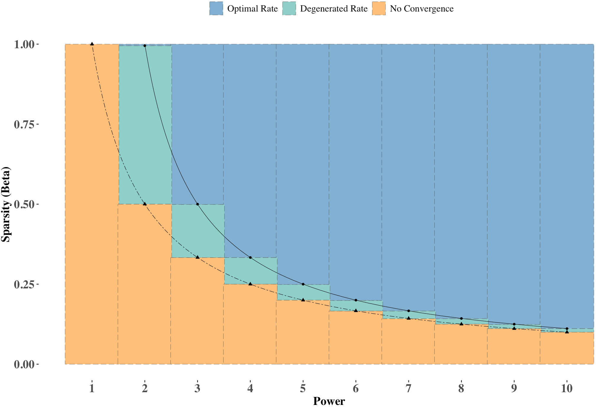
Here denote for some fixed . Eq. (4.2) implies a phase transition for and as changes. Recall that is the matrix whose columns are the (exact) leading singular vectors of and Eq. (4.1) together with the Davis-Kahan theorem implies with high probability. On the other hand, it has recently been shown that with high probability ; see e.g., [75, 21]. Therefore if then both and converges to at the same rates as and , up to some logarithmic factors. Meanwhile, if then and converge to at the slower rates of and , repectively. Convergences of and are not guaranteed when . These different convergence rates can be motivated by the observation that, since is a binary matrix, the main thing that changes when decreases is the number of non-zero entries in . In other words, we are estimating the leading singular vectors of using a noisy realization that, when decreases, contains less information about . It is thus unlikely that any fixed value of will work uniformly well for all values of . Indeed, as we will see in Theorem 4.1 and Section S.1.1, both of the thresholds and in Eq. (4.2) are necessary and sufficient. We now provide three examples illustrating the relationships between and ; see also the visual summary in Figure 1.
-
•
First consider the dense regime with . Then is sufficient for to attain the optimal rate ; and for to attain the optimal rate . No convergence is guaranteed when .
-
•
Next consider a semi-sparse regime with . For , the optimal rate is attained when , the sub-optimal rate is attained when . For , the optimal rate is attained when , the sub-optimal rate is attained when . No convergence is guaranteed when .
-
•
Finally consider a semi-sparse regime with . For , the optimal rate is attained when . For , the optimal rate is attained when . No convergence is guaranteed when .
In summary, the above discussions provide theoretical justification to the well-known advice that choosing a slightly larger and are essential to the success of RSVD in practical applications [86].
4.2 Lower bound and phase transition sharpness
We now study the sharpness of the phase transition thresholds described in Section 4.1. More specifically, we derive lower bounds for and , and thereby show that the conditions and are both necessary and sufficient for and to converge to , at either the slow rate or the optimal rate shown in Eq. (4.2), respectively.
The lower bounds for and depend on the following assumption on the growth rate of , namely that for any finite there exists some fixed constant such that,
| (4.3) |
We now clarify Eq. (4.3). Suppose is a Wigner matrix whose entries are independent mean random variables with equal variances given by . Then satisfy Eq. (4.3) using the well-known “trace method” combinatorial arguments from random matrix theory; see e.g. Lemma 1.5 in [15] for more details. Eq. (4.3) and Eq. (4.1) are therefore satisfied for Erdős–Rényi graphs. By adapting the trace method arguments for Wigner matrices, we can show that Eq. (4.3) continues to hold for any edge-independent random graphs with homogeneous variances, i.e., satisfies for all , or equivalently, that for all . In other words, Eq. (4.3) is satisfied by stochastic blockmodel graphs and their degrees-corrected and/or mixed membership variants, and by (generalized) random dot product graphs.
Theorem 4.1.
Assume the setting of Theorem 3.2 and further suppose: (i) and for some fixed constant ; (ii) there exists a constant not depending on but can depend on such that , (iii) . Choose and . Let be fixed but arbitrary. Then there exists a constant depending only on such that, with probability approaching , we have
Remark 4.1.
For simplicity we had presented Theorem 4.1 in the case where . An almost identical lower bound is available for the case where , provided that we replaced the term in the above expressions with a term.
For ease of exposition we will ignore any logarithmic factor of in the following discussion. We see that the lower bounds in Theorem 4.1 match the upper bounds in Eq. (4.2) for both the no convergence regime where and the sub-optimal regime where ; recall that if then and has the same convergence rate as and , respectively, and are thus rate-optimal. Here we note that in Theorem 4.1, when is equivalent to showing no convergence as . See Section S.1.1 in the Supplemenatry File for simulation results illustrating these upper and lower bounds for both and . Finally we emphasize Theorem 4.1 is stated in a more general setting than that for random graphs, e.g., the lower bound holds whenever is a random symmetric Gaussian matrix provided that with high probability and satisfies Eq.(4.3).
4.3 Exact recovery for stochastic blockmodels
We now apply the bound for and given in Eq. (4.2), to the problem of community detection in stochastic blockmodel graphs [63], one of the most popular generative model for network data with an assumed intrinsic community structure. We first recall the definition of stochastic blockmodel graphs.
Definition 1 (SBM).
Let be a positive integer and let be positive vector satisfying . Let be a symmetric matrix whose entries are in . We say that is a -blocks stochastic blockmodel (SBM) graph with parameters and , and sparsity factor , if the following holds. First where the are iid with for all . Then is a symmetric binary matrix such that, conditioned on , for all the are independent Bernoulli random variables with .
Community detection is well-studied (see e.g., the surveys [53, 1]), with many available techniques including those based on maximizing modularity and likelihood [14, 92, 110], random walks [96, 102], semidefinite programming [57, 2], and spectral clustering [121]. In particular spectral clustering using the adjacency matrix is a simple and popular community detection algorithm wherein, given , we first choose an embedding dimension and compute the matrix of eigenvectors corresponding to the largest (in modulus) eigenvalues of . Next we cluster the rows of into cluster using either the -means or -medians algorithms and let be the resulting cluster membership for the th row of . The motivation behind spectral clustering is that for stochastic blockmodel graphs (1) serves as an estimate for the leading eigenvectors of the underlying edge probabilities matrix and (2) the rows of contain all of the necessary information for recovering , i.e., there exists a collection of distinct vectors such that for all .
Statistical properties of spectral clustering had been widely studied in recent years, see e.g., [113, 99, 76, 67, 82, 112, 75, 3, 74] for an incomplete list of references. In particular it is well-known that spectral clustering will, with high probability, exactly recover the community assignment for SBM graphs as well as its variants including degree-corrected SBM [69] and popularity adjusted SBM [108], i.e., spectral clustering yields a such that with high probability there exists a permutation of for which for all .
In many real-world applications like social or biological networks, the number of nodes can be on the order of , see e.g. [56]. As a result, the computation of in spectral clustering using standard SVD algorithms can be prohibitively demanding in terms of both the computational time and memory requirement. Under our rs-RSVD framework, by taking as the observed matrix we propose an economical spectral clustering procedure (see Algorithm 2) that replaces by its approximation produced by rs-RSVD. We note that the time complexity of Algorithm 2 is on the order of operations and only require enough memory to store the non-zero elements of . These time and memory requirements can be considerably smaller than that of the standard spectral clustering, especially for large and non-dense graphs.
The following result shows that for a fixed depending on the sparsity of , Algorithm 2 will, with high probability, also exactly recovers
Theorem 4.2.
Let be a -blocks SBM with sparse parameter where for all and for some . Let and suppose that is given by Algorithm 2 wherein we choose: (i) , (ii) for some universal constant and (iii) . Then for sufficiently large , we have that exactly recovers with probability at least .
Remark 4.2.
In practice one may consider clustering with the -approximate -medians algorithm when implementing Algorithm 2, instead of the exact -median algorithm which is NP-hard [87]. See e.g. [76] for a more detailed discussion comparing the -approximate -medians and the exact -medians algorithms. Theorem 4.2 still holds for approximate -medians.
Remark 4.3.
Community detection using RSVD was also studied in [130]. In particular, Theorem 1 in [130] shows that if then weak recovery is possible using , provided that one choose and for any fixed but arbitrary . Recall that weak recovery only requires the proportion of mis-clustered vertices to converge to . Comparing the two results, we see the sparsity condition in [130] is less stringent than the condition in Theorem 4.2 while the exact recovery with fixed in Theorem 4.2 is a much stronger guarantee (and also is more computationally efficient) than weak recovery in [130].
The proof of Theorem 4.2 is based on the perturbation bounds given in Eq. (4.2). More specifically, if then, with high probability,
| (4.4) |
If Eq. (4.4) holds then the arguments for exact recovery of using can be easily adapted to show exact recovery using ; see the proof of Theorem 2.6 in [82] or the proof of Theorem 5.2 in [75] for some examples of these types of arguments. Furthermore, while is sufficient to show exact recovery using when is not an integer, in practice we recommend choosing the slightly larger value of . Indeed, as shown in Section 4.2, the convergence rate for when is generally faster than that for , and this can lead to better finite-sample performance.
Theorem 4.2 also indicates that smaller values of will require larger number of power iterations and hence the computational cost of Algorithm 2 increases as the graphs become sparser. In other words, there is an inherent trade-off between the sparsity of the network and the computation cost needed to approximate its eigenvectors. In addition, as we allude to earlier in Remark 4.3, Algorithm 2 does not guarantee exact recovery of in the very sparse asymptotic regime where and this is due entirely to the use of , as an approximation for . More specifically, if then [112, 75, 3] showed that exact recovery of is possible using . In contrast, by Theorem 4.1, we see that neither nor converge to for any finite . Hence, to guarantee exact recovery, we will need to let grows with and this will require a more careful analysis of Algorithm 1 to remove the effect of the condition number when . More specifically, instead of estimating all leading singular vectors simultaneously, we might need to estimate these singular vectors in stages, starting from the first leading singular vector. After each stage we will project onto the orthogonal complement of the singular vectors estimated thus far before proceeding with the estimation of the singular vectors in the next stage. Finally, while it is certainly the case that, asymptotically, for any , in practice for all . Hence, while asymptotic results in the regime are interesting, they need not lead to better understanding of RSVD for practical applications.
4.4 Normal approximation for
We now consider the row-wise fluctuations of . Recall the setting at the beginning of this section where is the adjacency matrix of an edge independent random graph whose edge probabilities matrix has rank matrix with bounded, and . Suppose furthermore that the entries of are homogeneous so that . Then and hence for all . In addition the are also homogeneous; here denote the diagonal elements of . As and has bounded condition number, we conclude that has bounded coherence, i.e., . The above conditions are satisfied for many random graph models including stochastic blockmodels and their degree-corrected and mixed-membership stochastic variants [63, 69] as well as (generalized) random dot product graphs [103, 128].
Recall Assumption 3. As , take . We now verify Eq (3.13). Note, where is the th entry of and is the th row of . For a fixed , the are independent mean random variables and hence, by the Lindeberg-Feller central limit theorem, we have
where is the matrix of the form
Note that is non-degenerate. Indeed, as is homogeneous, we have
for some fixed constant . In summary, Assumption 3 is satisfied and we have the following normal approximations for the row-wise fluctuations of , namely there exists a sequence of orthogonal matrices such that for any fixed index ,
as . This result was derived previously in [103, 52, 21, 42]; see for example Theorem 2.8 in [42]. Theorem 3.4 implies the same limiting distribution for , i.e., for any there exists a sequence of orthogonal matrix such that
as . See Section S.1.1.3 for a numerical illustration of this convergence.
5 Additional applications
In this section we apply our main theorems to two other high-dimensional statistical problems, namely, symmetric matrix completion and PCA with missing data. For both of these problems we show that the error rates achieved by the approximate singular vectors is (almost) identical to that for the exact singular vectors of the noisily observed matrices.
5.1 Matrix completion with noises
Let be a matrix whose entries are only partially and noisily observed. Such matrix occurs in many real-world applications, including the famous Netflix challenge [98]. As another example, if is an Euclidean distance matrix (EDM) between points in then and it is commonly the case that is noisily observed [8, 54, 40, 65]. Finally, if is a signal correlation matrix between multiple remote sensors [107] then is usually only partial observed due to power constraints [31].
For this paper we assume that is symmetric, rank , and we observed
| (5.1) |
Here is an unobserved noise matrix, is a symmetric binary matrix, and denote the Hadamard product. The matrix and induces noise and missingness in the entries of , respectively. We shall assume, for ease of exposition, that the (upper triangle) entries of are iid random variables while the (upper triangular) entries of are iid Bernoulli random variables with success probability . The aim of matrix completion is to recover from . Since , one simple and widely used estimate for is given by where is the truncated rank- SVD of ; see [3, 28, 70, 23, 19] and the references therein.
In many real-world applications, the dimensions of can be rather large and yet can be quite sparse compared to , i.e., the number of non-zero entries of is much smaller than . It is thus computationally attractive to approximate the left singular vectors of using randomized algorithms such as rs-RSVD. More specifically, let be the output of Algorithm 1 with for some properly specified choices of and . We view as an approximation for , and thus as an estimate of . Given we compute a rank- approximation for via . We can then take as an estimate for or, in the event that we desire symmetry, take as an estimate for . The resulting algorithm, termed RSVD-based matrix completion, is presented in Algorithm 3.
Using the and perturbation results in Theorem 3.2 and 3.3 and the entrywise concentration in Corollary 3.2, we derive the error bounds for the estimates and . Furthermore, by extending Theorem 3.4, we establish the general entrywise limiting distribution for the RSVD-based low-rank approximation , in Theorem S.6.1 of the supplementary document. This result allows us to construct confidence interval for any with . For ease of exposition we shall assume that both and are bounded, and that is known. These are typical assumptions in the literature. If is unknown then, as the entries of are assumed to be missing completely at random, it can be consistently estimated by calculating the proportion of missing entries among all the entries in . The resulting converges to at the rate of and has no effect on the theoretical results in Theorem 5.1
Theorem 5.1.
Let be a symmetric matrix with . Let be a noisily observed version of generated according to Eq. (5.1) for some known value of . Suppose there exists constants and such that
| and | (5.2) |
Let and be obtained from Algorithm 3 wherein we chose: (i) ; (ii) and (iii) . Denote .
-
(Error Bounds)
We then have, with probability at least , that
(5.3) where is as defined in the statement of Theorem 3.3.
-
(Entrywise limiting distribution)
Suppose, in addition to the above assumptions, that is homogeneous, i.e., . Let and denote the variance of by
(5.4) Choose and as above and let . Then for any given pair , we have
(5.5) as . Furthermore, for any finite set of indices , the collection of random variables are (asymptotically) mutually independent.
-
(Entrywise confidence interval)
Suppose above assumptions hold. Let . Define the RSVD-based estimate of by
(5.6) where . Then for any indices pair we have
(5.7)
We now compare Theorem 5.1 with existing results in the literature. Recall that the prototypical spectral estimate for is given by where is the truncated rank- SVD of ; for conciseness we refer to as the deterministic SVD-based estimator for . First suppose that Eq. (5.2) holds for some constants and . We then have
| (5.8) | ||||
with high probability. The above bound for is from Theorem 1.1 and Theorem 1.3 of [70] while the remaining bounds in Eq. (5.8) are from Theorem 3.4 of [3].
Now consider the bounds for and given in Theorem 5.1. For ease of presentation we choose and . These choices for and allow us to set and for any arbitrary . Eq. (5.3) then implies
| (5.9) | ||||
with high probability. Comparing Eq. (5.8) and Eq. (5.9) we see that the -RSVD estimate achieves the same Frobenius norm error rate as that for the deterministic SVD estimate . Note that the Frobenius norm error for is rate-optimal whenever [19, 3]. The max-norm error rate for is also almost identical to that of with the only difference being the extra factor for ; here is an arbitrary positive constant. Similarly, converges to at the same rate as up to the factor. These extra factors for can be removed with more careful book keeping; see Remark 3.5 for more details. If is either bounded or diverge at a slower rate than , or when , then Eq. (5.9) still holds but with the factor replaced by a factor for some finite .
We next discuss the limiting distributions and confidence intervals given in Theorem 5.1. We had assumed that is homogeneous; this assumption was also used in Theorem 4.12 in [28] for the estimator . The main role of the homogeneity assumption is to guarantee that the entrywise noise levels are roughly on the same order, and thereby simplify the statement of Theorem 5.1. Similar assumption are also used in the distributional theory for PCA with missing data; see e.g. Assumption 1 in [125]. Our general result, namely Theorem S.6.1, does not require to be homogenous. The condition in Theorem 5.1 is then similar to that in Theorem 3.4 for the row-wise limiting distribution of , i.e., we need to guarantee that the entrywise fluctuation of is asymptotically equivalent to the entrywise fluctuation of . For any given pair , we can thus quantify the uncertainty of the by constructing the confidence interval:
where is the quantile of . The resulting confidence interval has (asymptotic) coverage of . We emphasize that the estimated variance are computed using only the rs-RSVD outputs and ; see Eq. (5.6).
Remark 5.1.
The conditions posited in Theorem 5.1 for the estimator is slightly more restrictive than those for in the current literature. Recall that from Eq. (5.2), we have for some arbitrary . Eq. (5.2) also implies a lower bound for the signal-to-noise ratio of the form
for some arbitrary . In contrast, the conditions for given in Theorem 3.4 of [3] is that and . The conditions and in Theorem 5.1 is analogous to the condition for exact recovery of SBM using . In particular for matrix completion using rs-RSVD to work in the and regime we will need to have diverging with and this requires a more careful analysis of RSVD to remove the effect of the condition number as increases. Furthermore, very large and/or diverging values of also reduces the effectiveness of RSVD procedures for large-scale matrix computations, especially when the matrices are too large to store in fast memory as it requires a possibly excessive number of passes through the data. Finally we note that depends on the parameters , , and . In particular, if is homogeneous (as assumed in [28]) so that , then and Eq. (5.2) simplifies to the condition that and hence .
5.2 PCA with missing data
We now consider principal components estimation with missing data. In particular we consider the following data generating mechanism from [18]:
| (5.10) |
Here is a data matrix with being -dimensional iid random vectors, is a matrix, is a matrix whose entries are iid random variables, and is a matrix whose entries are iid random variables. We emphasize that , and are mutually independent. We can see that the rows of are iid random vectors with mean and covariance matrix . We denote the SVD of by where and ; the columns of are leading principal components.
Due to sampling issues and/or privacy-preserving intention, it is often the case that only a partial subset of the entries in are observed. More specifically let be a binary matrix whose entries are iid Bernoulli random variables with success probability . Then, instead of observing , we only observed where denote the Hadamard product between matrices. Given an observed , [18] propose the following spectral procedure for recovering the principle components . First form the symmetric matrix
| (5.11) |
where sets diagonal entries of the corresponding matrix to zero. Next compute the matrix whose columns are the left singular vectors corresponding to the largest singular values of ; serves as an estimate of . The authors of [18] then derive high-probability error bounds for and .
As the dimension can be reasonably large compared to the number of samples while the number of non-zero entries in can be much smaller than , we consider replacing the singular vectors of by the approximate singular vectors computed using RSVD; see Algorithm 4. The following result shows that by choosing either or , the approximate singular vectors achieve the same estimation rate as that for given in [18]. For ease of presentation, and following [18], we shall assume that has a bounded condition number, i.e., .
Theorem 5.2.
Suppose is a matrix generated according to Eq. (5.10). Let denote the coherence parameter for and let . Suppose there exist constants and such that and satisfies the sample size condition
| (5.12) |
Define and
| (5.13) |
Suppose that for some . Let be generated via Algorithm 4, wherein we choose: (i) for any fixed ; (ii) and (iii) . Then with probability at least , we have
Remark 5.2.
The assumption of bounded is widely considered in the literature, see e.g., the discussion prior to Eq.(4.17) in [18] and see also [109, 64, 25, 29]. For example, is satisfied with high-probability when is generated from a standard Gaussian matrix (see e.g. [119]). Note that the sample size requirement in Eq. (5.12) is exactly the same as that in Eq. (4.14) of [18] for bounded . If grows with then the sample size requirement in Eq. (5.12) depend on polynomial factors of and these factors can be extracted from the proof of Theorem 5.2 with a bit more careful book-keeping.
Remark 5.3.
Comparing the Theorem 5.2 with Corollary 4.3 in [18], we see that there exists a finite such that and converges to at the same rate , up to a factor; furthermore this logarithmic gap can be removed by choosing . The condition in Theorem 5.2 indicates that an appropriate value for will depend on the relationship between and , e.g., larger dimensions (compared to ) will require larger power iterations . In particular, suppose and for some ; here is necessary for Eq. (5.12) to hold. Then from the definition in Eq. (5.13), we have, after some straightforward algebra, that
To attain the rate in Eq. (5.13), we thus need where is any small constant.
We note that Theorem 5.2 only provides perturbation bound for and not more refined results such as perturbation bound for . This omission is due mainly to the noise structure in the matrix . More specifically if we take and view as the noisily observed version of then is of the form
The (upper triangular) entries of are therefore not mutually independent and this leads to non-trivial technical challenges in deriving bounds for . In particular, Assumption 2 need not hold. In contrast, existing bounds for are based on leave-two-out analysis which is a variant of leave-one-out analysis; see Appendix G in [125]. Similar to the discussion in Remark 3.6, this leave-two-out approach is not directly applicable to the analysis of because depends on and the entrywise dependency structure in is more complicated than that in .
Recent work show that we can estimate the principal components by using the leading left singular vectors of directly (as opposed to which uses the leading eigenvectors of ); the resulting estimate has and error bounds that are comparable to those for in the regime where either or is not much larger (in magnitude) compared to ; see Section 3.2 in [125] for more details. Note that is a rectangular matrix whose entries, conditional on , are mutually independent. We can thus apply the results for asymmetric -RSVD in Section S.2 in the Supplementary File, to derive perturbation bounds for the approximate singular vectors of . A sketch of this argument is given below.
Let be the leading singular vectors of and let be the rs-RSVD approximation of obtained from Algorithm 5 for . Then where denote the expectation with respect to only. Define, with a slight abuse of notation,
Denote and . Then satisfies Assumption S.1 with ; see Lemma 1 in [125]. Now suppose for some constant . Then also satisfies Assumption S.2; this claim follows from Remark S.2.2. Theorem S.2.1 then yields upper bounds for and when ; these bounds are the same, up to some logarithmic factors, as those given in Lemmas 1–4 and Theorem 1 of [125] for and .
6 Discussions
In this paper we analyzed the statistical behavior of RSVD algorithms under the assumption that the observed matrix is generated according to a low-rank “signal-plus-noise” model. In particular, we derived and perturbation bounds for , entrywise concentration bounds for , and normal approximations for the row-wise fluctuations of . There are several directions to pursue for the future research. Firstly, our upper and lower bounds for and include factors depending on the rank , condition number and other logarithmic terms. These factors are generally sub-optimal and can be sharpened with a more refined analysis; see for example Remark 3.5 and the discussion after Theorem 4.2. Secondly, as we shown in Section 4.2, our and bounds and the corresponding phase transition are sharp whenever satisfies a certain trace growth condition. This condition is satisfied in the context of random graphs inference and it is of some interest to find other statistical inference problem where this condition also holds. Thirdly, the theoretical results of this paper currently assume that is bounded and that and are either bounded or slowly growing. It is thus natural to extend these results to more general settings, such as when grows with at rate for some , when the noise matrix has more complicated entrywise dependence structure, when the SNR is only of order for some , or when . We note that these extensions are related, e.g., for some will, in general, require for consistent estimation of using . Fourthly, while subspace power iterations (as considered in this paper) is one of the most popular approach for RSVD, there are other approaches such as those based on Krylov subspaces [89] and perturbation bounds in and for RSVD using Krylov subspaces may require quite different techniques than those presented here. Finally, many modern dataset are represented as tensors and are analyzed using higher-order SVD; these procedures generally flatten tensor data into matrices across different dimensions and then compute the truncated SVD of the resulting flattened matrices [39, 131]. Statistical analysis of RSVD in the context of noisy tensor data is thus of some theoretical and practical interest. {supplement} \stitleSupplementary File for “Perturbation Analysis of Randomized SVD and its Applications to High-dimensional Statistics” \sdescriptionThe Supplementary File contains numerical experiments, additional theoretical results, and all technical lemmas and proofs.
References
- Abbe [2017] {barticle}[author] \bauthor\bsnmAbbe, \bfnmEmmanuel\binitsE. (\byear2017). \btitleCommunity detection and stochastic block models: recent developments. \bjournalJournal of Machine Learning Research \bvolume18 \bpages6446–6531. \endbibitem
- Abbe, Bandeira and Hall [2016] {barticle}[author] \bauthor\bsnmAbbe, \bfnmE.\binitsE., \bauthor\bsnmBandeira, \bfnmA. S.\binitsA. S. and \bauthor\bsnmHall, \bfnmG.\binitsG. (\byear2016). \btitleExact recovery in the stochastic blockmodel. \bjournalIEEE Transactions on Information Theory \bvolume62 \bpages471–487. \endbibitem
- Abbe et al. [2020] {barticle}[author] \bauthor\bsnmAbbe, \bfnmEmmanuel\binitsE., \bauthor\bsnmFan, \bfnmJianqing\binitsJ., \bauthor\bsnmWang, \bfnmKaizheng\binitsK. and \bauthor\bsnmZhong, \bfnmYiqiao\binitsY. (\byear2020). \btitleEntrywise eigenvector analysis of random matrices with low expected rank. \bjournalThe Annals of Statistics \bvolume48 \bpages1452–1474. \endbibitem
- Achlioptas and McSherry [2007] {barticle}[author] \bauthor\bsnmAchlioptas, \bfnmDimitris\binitsD. and \bauthor\bsnmMcSherry, \bfnmFrank\binitsF. (\byear2007). \btitleFast computation of low-rank matrix approximations. \bjournalJournal of the ACM \bvolume54. \endbibitem
- Ahlswede and Winter [2002] {barticle}[author] \bauthor\bsnmAhlswede, \bfnmR.\binitsR. and \bauthor\bsnmWinter, \bfnmA.\binitsA. (\byear2002). \btitleStrong converse for identification via quantum channels. \bjournalIEEE Transactions on Information Theory \bvolume48 \bpages569–579. \endbibitem
- Ahn and Horenstein [2013] {barticle}[author] \bauthor\bsnmAhn, \bfnmS. C.\binitsS. C. and \bauthor\bsnmHorenstein, \bfnmA.\binitsA. (\byear2013). \btitleEigenvalue ratio test for the number of factors. \bjournalEconometrica \bvolume81 \bpages1203–1227. \endbibitem
- Airoldi et al. [2008] {barticle}[author] \bauthor\bsnmAiroldi, \bfnmE. M.\binitsE. M., \bauthor\bsnmBlei, \bfnmD. M.\binitsD. M., \bauthor\bsnmFienberg, \bfnmS. E.\binitsS. E. and \bauthor\bsnmXing, \bfnmE. P.\binitsE. P. (\byear2008). \btitleMixed membership stochastic blockmodels. \bjournalJournal of Machine Learning Research \bvolume9 \bpages1981–2014. \endbibitem
- Alfakih, Khandani and Wolkowicz [1999] {barticle}[author] \bauthor\bsnmAlfakih, \bfnmAbdo Y\binitsA. Y., \bauthor\bsnmKhandani, \bfnmAmir\binitsA. and \bauthor\bsnmWolkowicz, \bfnmHenry\binitsH. (\byear1999). \btitleSolving Euclidean distance matrix completion problems via semidefinite programming. \bjournalComputational Optimization and Applications \bvolume12 \bpages13–30. \endbibitem
- Askham and Kutz [2018] {barticle}[author] \bauthor\bsnmAskham, \bfnmTravis\binitsT. and \bauthor\bsnmKutz, \bfnmJ Nathan\binitsJ. N. (\byear2018). \btitleVariable projection methods for an optimized dynamic mode decomposition. \bjournalSIAM Journal on Applied Dynamical Systems \bvolume17 \bpages380–416. \endbibitem
- Athreya et al. [2021] {barticle}[author] \bauthor\bsnmAthreya, \bfnmAvanti\binitsA., \bauthor\bsnmTang, \bfnmMinh\binitsM., \bauthor\bsnmPark, \bfnmYoungser\binitsY. and \bauthor\bsnmPriebe, \bfnmCarey E\binitsC. E. (\byear2021). \btitleOn estimation and inference in latent structure random graphs. \bjournalStatistical Science \bvolume36 \bpages68–88. \endbibitem
- Bandeira and Van Handel [2016] {barticle}[author] \bauthor\bsnmBandeira, \bfnmAfonso S\binitsA. S. and \bauthor\bsnmVan Handel, \bfnmRamon\binitsR. (\byear2016). \btitleSharp nonasymptotic bounds on the norm of random matrices with independent entries. \bjournalAnnals of Probability \bvolume44 \bpages2479–2506. \endbibitem
- Belkin and Niyogi [2003] {barticle}[author] \bauthor\bsnmBelkin, \bfnmM.\binitsM. and \bauthor\bsnmNiyogi, \bfnmP.\binitsP. (\byear2003). \btitleLaplacian eigenmaps for dimensionality reduction and data representation. \bjournalNeural Computation \bvolume15 \bpages1373-1396. \endbibitem
- Berend and Tassa [2010] {barticle}[author] \bauthor\bsnmBerend, \bfnmD.\binitsD. and \bauthor\bsnmTassa, \bfnmT.\binitsT. (\byear2010). \btitleImproved Bounds on Bell Numbers and on Moments of Sums of Random Variables. \bjournalProbability and Mathematical Statistics \bvolume30 \bpages185–205. \endbibitem
- Bickel and Chen [2009] {barticle}[author] \bauthor\bsnmBickel, \bfnmP. J.\binitsP. J. and \bauthor\bsnmChen, \bfnmA.\binitsA. (\byear2009). \btitleA nonparametric view of network models and Newman-Girvan and other modularities. \bjournalProceedings of the National Academy of Sciences of the United States of America \bvolume106 \bpages21068–21073. \endbibitem
- Bordenave [2019] {bmisc}[author] \bauthor\bsnmBordenave, \bfnmCharles\binitsC. (\byear2019). \btitleLectures on random matrix theory. \bnoteavailable online at https://www.math.univ-toulouse.fr/~bordenave/IMPA-RMT.pdf. \endbibitem
- Cai, Ma and Wu [2013] {barticle}[author] \bauthor\bsnmCai, \bfnmT Tony\binitsT. T., \bauthor\bsnmMa, \bfnmZongming\binitsZ. and \bauthor\bsnmWu, \bfnmYihong\binitsY. (\byear2013). \btitleSparse PCA: Optimal rates and adaptive estimation. \bjournalThe Annals of Statistics \bvolume41 \bpages3074–3110. \endbibitem
- Cai and Zhang [2018] {barticle}[author] \bauthor\bsnmCai, \bfnmT Tony\binitsT. T. and \bauthor\bsnmZhang, \bfnmAnru\binitsA. (\byear2018). \btitleRate-optimal perturbation bounds for singular subspaces with applications to high-dimensional statistics. \bjournalThe Annals of Statistics \bvolume46 \bpages60–89. \endbibitem
- Cai et al. [2021] {barticle}[author] \bauthor\bsnmCai, \bfnmChangxiao\binitsC., \bauthor\bsnmLi, \bfnmGen\binitsG., \bauthor\bsnmChi, \bfnmYuejie\binitsY., \bauthor\bsnmPoor, \bfnmH Vincent\binitsH. V. and \bauthor\bsnmChen, \bfnmYuxin\binitsY. (\byear2021). \btitleSubspace estimation from unbalanced and incomplete data matrices: statistical guarantees. \bjournalThe Annals of Statistics \bvolume49 \bpages944–967. \endbibitem
- Candes and Plan [2010] {barticle}[author] \bauthor\bsnmCandes, \bfnmEmmanuel J\binitsE. J. and \bauthor\bsnmPlan, \bfnmYaniv\binitsY. (\byear2010). \btitleMatrix completion with noise. \bjournalProceedings of the IEEE \bvolume98 \bpages925–936. \endbibitem
- Candes and Recht [2009] {barticle}[author] \bauthor\bsnmCandes, \bfnmE. J.\binitsE. J. and \bauthor\bsnmRecht, \bfnmB.\binitsB. (\byear2009). \btitleExact matrix completion via convex optimization. \bjournalFoundations of Computational Mathematics \bvolume9 \bpages717–772. \endbibitem
- Cape, Tang and Priebe [2019a] {barticle}[author] \bauthor\bsnmCape, \bfnmJ.\binitsJ., \bauthor\bsnmTang, \bfnmM.\binitsM. and \bauthor\bsnmPriebe, \bfnmC. E.\binitsC. E. (\byear2019a). \btitleSignal-plus-noise matrix models: eigenvector deviations and fluctuations. \bjournalBiometrika \bvolume106 \bpages243–250. \endbibitem
- Cape, Tang and Priebe [2019b] {barticle}[author] \bauthor\bsnmCape, \bfnmJoshua\binitsJ., \bauthor\bsnmTang, \bfnmMinh\binitsM. and \bauthor\bsnmPriebe, \bfnmCarey E\binitsC. E. (\byear2019b). \btitleThe two-to-infinity norm and singular subspace geometry with applications to high-dimensional statistics. \bjournalThe Annals of Statistics \bvolume47 \bpages2405–2439. \endbibitem
- Chatterjee [2015] {barticle}[author] \bauthor\bsnmChatterjee, \bfnmSourav\binitsS. (\byear2015). \btitleMatrix estimation by universal singular value thresholding. \bjournalThe Annals of Statistics \bvolume43 \bpages177–214. \endbibitem
- Chen, Cheng and Fan [2021] {barticle}[author] \bauthor\bsnmChen, \bfnmYuxin\binitsY., \bauthor\bsnmCheng, \bfnmChen\binitsC. and \bauthor\bsnmFan, \bfnmJianqing\binitsJ. (\byear2021). \btitleAsymmetry helps: Eigenvalue and eigenvector analyses of asymmetrically perturbed low-rank matrices. \bjournalThe Annals of Statistics \bvolume49 \bpages435–458. \endbibitem
- Chen, Guibas and Huang [2014] {binproceedings}[author] \bauthor\bsnmChen, \bfnmYuxin\binitsY., \bauthor\bsnmGuibas, \bfnmLeonidas\binitsL. and \bauthor\bsnmHuang, \bfnmQixing\binitsQ. (\byear2014). \btitleNear-Optimal Joint Object Matching via Convex Relaxation. In \bbooktitleProceedings of the 31st International Conference on Machine Learing \bpages100–108. \endbibitem
- Chen and Suh [2015] {binproceedings}[author] \bauthor\bsnmChen, \bfnmYuxin\binitsY. and \bauthor\bsnmSuh, \bfnmChangho\binitsC. (\byear2015). \btitleSpectral MLE: Top-k rank aggregation from pairwise comparisons. In \bbooktitleProceedings of the 32nd International Conference on Machine Learning \bpages371–380. \endbibitem
- Chen et al. [2019] {barticle}[author] \bauthor\bsnmChen, \bfnmYuxin\binitsY., \bauthor\bsnmFan, \bfnmJianqing\binitsJ., \bauthor\bsnmMa, \bfnmCong\binitsC. and \bauthor\bsnmWang, \bfnmKaizheng\binitsK. (\byear2019). \btitleSpectral method and regularized MLE are both optimal for top- ranking. \bjournalThe Annals of Statistics \bvolume47 \bpages2204–2235. \endbibitem
- Chen et al. [2021a] {barticle}[author] \bauthor\bsnmChen, \bfnmYuxin\binitsY., \bauthor\bsnmChi, \bfnmYuejie\binitsY., \bauthor\bsnmFan, \bfnmJianqing\binitsJ. and \bauthor\bsnmMa, \bfnmCong\binitsC. (\byear2021a). \btitleSpectral Methods for Data Science: A Statistical Perspective. \bjournalFoundations and Trends® in Machine Learning \bvolume14 \bpages566–806. \endbibitem
- Chen et al. [2021b] {barticle}[author] \bauthor\bsnmChen, \bfnmYuxin\binitsY., \bauthor\bsnmFan, \bfnmJianqing\binitsJ., \bauthor\bsnmMa, \bfnmCong\binitsC. and \bauthor\bsnmYan, \bfnmYuling\binitsY. (\byear2021b). \btitleBridging convex and nonconvex optimization in robust PCA: Noise, outliers and missing data. \bjournalThe Annals of Statistics \bvolume49 \bpages2948–2971. \endbibitem
- Cheng, Wei and Chen [2021] {barticle}[author] \bauthor\bsnmCheng, \bfnmChen\binitsC., \bauthor\bsnmWei, \bfnmYuting\binitsY. and \bauthor\bsnmChen, \bfnmYuxin\binitsY. (\byear2021). \btitleTackling small eigen-gaps: Fine-grained eigenvector estimation and inference under heteroscedastic noise. \bjournalIEEE Transactions on Information Theory \bvolume67 \bpages7380–7419. \endbibitem
- Cheng et al. [2012] {barticle}[author] \bauthor\bsnmCheng, \bfnmJie\binitsJ., \bauthor\bsnmYe, \bfnmQiang\binitsQ., \bauthor\bsnmJiang, \bfnmHongbo\binitsH., \bauthor\bsnmWang, \bfnmDan\binitsD. and \bauthor\bsnmWang, \bfnmChonggang\binitsC. (\byear2012). \btitleSTCDG: An efficient data gathering algorithm based on matrix completion for wireless sensor networks. \bjournalIEEE Transactions on Wireless Communications \bvolume12 \bpages850–861. \endbibitem
- Coifman and Lafon [2006] {barticle}[author] \bauthor\bsnmCoifman, \bfnmR.\binitsR. and \bauthor\bsnmLafon, \bfnmS.\binitsS. (\byear2006). \btitleDiffusion maps. \bjournalApplied and Computational Harmonic Analysis \bvolume21 \bpages5–30. \endbibitem
- Cormode et al. [2011] {barticle}[author] \bauthor\bsnmCormode, \bfnmGraham\binitsG., \bauthor\bsnmGarofalakis, \bfnmM.\binitsM., \bauthor\bsnmHaas, \bfnmP. J.\binitsP. J. and \bauthor\bsnmJermaine, \bfnmC.\binitsC. (\byear2011). \btitleSynopses for massive data: samples, histogram, wavelets, sketches. \bjournalFoundations and Trends in Databases \bvolume4 \bpages1–294. \endbibitem
- Damle and Sun [2020] {barticle}[author] \bauthor\bsnmDamle, \bfnmA.\binitsA. and \bauthor\bsnmSun, \bfnmY.\binitsY. (\byear2020). \btitleUniform bounds for invariant subspace perturbations. \bjournalSIAM Journal on Matrix Analysis and Applications \bvolume41 \bpages1208–1236. \endbibitem
- d’Aspremont, Cucuringu and Tyagi [2021] {barticle}[author] \bauthor\bsnmd’Aspremont, \bfnmAlexandre\binitsA., \bauthor\bsnmCucuringu, \bfnmMihai\binitsM. and \bauthor\bsnmTyagi, \bfnmHemant\binitsH. (\byear2021). \btitleRanking and synchronization from pairwise measurements via SVD. \bjournalJournal of Machine Learning Research \bvolume22 \bpages1–63. \endbibitem
- Davenport and Romberg [2016] {barticle}[author] \bauthor\bsnmDavenport, \bfnmMark A\binitsM. A. and \bauthor\bsnmRomberg, \bfnmJustin\binitsJ. (\byear2016). \btitleAn overview of low-rank matrix recovery from incomplete observations. \bjournalIEEE Journal of Selected Topics in Signal Processing \bvolume10 \bpages608–622. \endbibitem
- Davidson and Szarek [2001] {binbook}[author] \bauthor\bsnmDavidson, \bfnmKenneth R\binitsK. R. and \bauthor\bsnmSzarek, \bfnmStanislaw J\binitsS. J. (\byear2001). \btitleHandbook of the geometry of Banach spaces, Vol. I \bchapterLocal operator theory, random matrices and Banach spaces, \bpages317-366. \bpublisherNorth-Holland. \endbibitem
- Davis and Kahan [1970] {barticle}[author] \bauthor\bsnmDavis, \bfnmChandler\binitsC. and \bauthor\bsnmKahan, \bfnmWilliam Morton\binitsW. M. (\byear1970). \btitleThe rotation of eigenvectors by a perturbation. III. \bjournalSIAM Journal on Numerical Analysis \bvolume7 \bpages1–46. \endbibitem
- De Lathauwer, De Moor and Vandewalle [2000] {barticle}[author] \bauthor\bsnmDe Lathauwer, \bfnmLieven\binitsL., \bauthor\bsnmDe Moor, \bfnmBart\binitsB. and \bauthor\bsnmVandewalle, \bfnmJoos\binitsJ. (\byear2000). \btitleOn the best rank- and rank- approximation of higher-order tensors. \bjournalSIAM Journal on Matrix Analysis and Applications \bvolume21 \bpages1324–1342. \endbibitem
- Ding et al. [2010] {barticle}[author] \bauthor\bsnmDing, \bfnmYichuan\binitsY., \bauthor\bsnmKrislock, \bfnmNathan\binitsN., \bauthor\bsnmQian, \bfnmJiawei\binitsJ. and \bauthor\bsnmWolkowicz, \bfnmHenry\binitsH. (\byear2010). \btitleSensor network localization, Euclidean distance matrix completions, and graph realization. \bjournalOptimization and Engineering \bvolume11 \bpages45–66. \endbibitem
- Drineas, Kannan and Mahoney [2006] {barticle}[author] \bauthor\bsnmDrineas, \bfnmPetros\binitsP., \bauthor\bsnmKannan, \bfnmRavi\binitsR. and \bauthor\bsnmMahoney, \bfnmMichael W\binitsM. W. (\byear2006). \btitleFast Monte Carlo algorithms for matrices II: Computing a low-rank approximation to a matrix. \bjournalSIAM Journal on Computing \bvolume36 \bpages158–183. \endbibitem
- Du and Tang [2021] {bunpublished}[author] \bauthor\bsnmDu, \bfnmX.\binitsX. and \bauthor\bsnmTang, \bfnmM.\binitsM. (\byear2021). \btitleHypothesis testing for equality of latent positions in random graphs. \bnotearXiv preprint at https://arxiv.org/abs/2105.10838. \endbibitem
- Edelman [1988] {barticle}[author] \bauthor\bsnmEdelman, \bfnmAlan\binitsA. (\byear1988). \btitleEigenvalues and condition numbers of random matrices. \bjournalSIAM Journal on Matrix Analysis and Applications \bvolume9 \bpages543–560. \endbibitem
- Edelman [1991] {barticle}[author] \bauthor\bsnmEdelman, \bfnmAlan\binitsA. (\byear1991). \btitleThe distribution and moments of the smallest eigenvalue of a random matrix of Wishart type. \bjournalLinear Algebra and its Applications \bvolume159 \bpages55–80. \endbibitem
- Eldar and Kutyniok [2012] {bbook}[author] \bauthor\bsnmEldar, \bfnmYonina C\binitsY. C. and \bauthor\bsnmKutyniok, \bfnmGitta\binitsG. (\byear2012). \btitleCompressed sensing: theory and applications. \bpublisherCambridge University Press. \endbibitem
- Eldridge, Belkin and Wang [2018] {binproceedings}[author] \bauthor\bsnmEldridge, \bfnmJustin\binitsJ., \bauthor\bsnmBelkin, \bfnmMikhail\binitsM. and \bauthor\bsnmWang, \bfnmYusu\binitsY. (\byear2018). \btitleUnperturbed: spectral analysis beyond Davis-Kahan. In \bbooktitleProceedings of Algorithmic Learning Theory \bpages321–358. \endbibitem
- Erdős and Rényi [1960] {barticle}[author] \bauthor\bsnmErdős, \bfnmPaul\binitsP. and \bauthor\bsnmRényi, \bfnmAlfréd\binitsA. (\byear1960). \btitleOn the evolution of random graphs. \bjournalPublications of the Mathematical Institute of the Hungarian Academy of Sciences \bvolume5 \bpages17–60. \endbibitem
- Erdős et al. [2013] {barticle}[author] \bauthor\bsnmErdős, \bfnmL.\binitsL., \bauthor\bsnmKnowles, \bfnmA.\binitsA., \bauthor\bsnmYau, \bfnmH. T.\binitsH. T. and \bauthor\bsnmYin, \bfnmJ.\binitsJ. (\byear2013). \btitleSpectral statistics of Erdős-Rényi graphs I: Local semicircle law. \bjournalAnnals of Probability \bvolume41 \bpages2279–2375. \endbibitem
- Erichson and Donovan [2016] {barticle}[author] \bauthor\bsnmErichson, \bfnmN Benjamin\binitsN. B. and \bauthor\bsnmDonovan, \bfnmCarl\binitsC. (\byear2016). \btitleRandomized low-rank dynamic mode decomposition for motion detection. \bjournalComputer Vision and Image Understanding \bvolume146 \bpages40–50. \endbibitem
- Fan, Liao and Mincheva [2013] {barticle}[author] \bauthor\bsnmFan, \bfnmJianqing\binitsJ., \bauthor\bsnmLiao, \bfnmYuan\binitsY. and \bauthor\bsnmMincheva, \bfnmMartina\binitsM. (\byear2013). \btitleLarge covariance estimation by thresholding principal orthogonal complements. \bjournalJournal of the Royal Statistical Society. Series B \bvolume75 \bpages603–647. \endbibitem
- Fan, Wang and Zhong [2018] {barticle}[author] \bauthor\bsnmFan, \bfnmJianqing\binitsJ., \bauthor\bsnmWang, \bfnmWeichen\binitsW. and \bauthor\bsnmZhong, \bfnmYiqiao\binitsY. (\byear2018). \btitleAn eigenvector perturbation bound and its application to robust covariance estimation. \bjournalJournal of Machine Learning Research \bvolume18 \bpages1–42. \endbibitem
- Fan et al. [2022+] {barticle}[author] \bauthor\bsnmFan, \bfnmJ.\binitsJ., \bauthor\bsnmFan, \bfnmY.\binitsY., \bauthor\bsnmHan, \bfnmX.\binitsX. and \bauthor\bsnmLv, \bfnmJ.\binitsJ. (\byear2022+). \btitleSIMPLE: Statistical Inference on Membership Profiles in Large Networks. \bjournalJournal of the Royal Statistical Society, Series B. \endbibitem
- Fortunato [2010] {barticle}[author] \bauthor\bsnmFortunato, \bfnmS.\binitsS. (\byear2010). \btitleCommunity detection in graphs. \bjournalPhysics Reports \bvolume486 \bpages75–174. \endbibitem
- Glunt, Hayden and Raydan [1993] {barticle}[author] \bauthor\bsnmGlunt, \bfnmW\binitsW., \bauthor\bsnmHayden, \bfnmTom L\binitsT. L. and \bauthor\bsnmRaydan, \bfnmMarcos\binitsM. (\byear1993). \btitleMolecular conformations from distance matrices. \bjournalJournal of Computational Chemistry \bvolume14 \bpages114–120. \endbibitem
- Golub and Van Loan [2013] {bbook}[author] \bauthor\bsnmGolub, \bfnmGene H\binitsG. H. and \bauthor\bsnmVan Loan, \bfnmCharles F\binitsC. F. (\byear2013). \btitleMatrix computations, \bedition3rd ed. \bpublisherJHU press. \endbibitem
- Gopalan and Blei [2013] {barticle}[author] \bauthor\bsnmGopalan, \bfnmPrem K\binitsP. K. and \bauthor\bsnmBlei, \bfnmDavid M\binitsD. M. (\byear2013). \btitleEfficient discovery of overlapping communities in massive networks. \bjournalProceedings of the National Academy of Sciences \bvolume110 \bpages14534–14539. \endbibitem
- Hajek, Wu and Xu [2016] {barticle}[author] \bauthor\bsnmHajek, \bfnmB.\binitsB., \bauthor\bsnmWu, \bfnmY.\binitsY. and \bauthor\bsnmXu, \bfnmJ.\binitsJ. (\byear2016). \btitleAcheiving exact cluster recovery threshold via semidefinite programming. \bjournalIEEE Transactions on Information Theory \bvolume62 \bpages2788–2797. \endbibitem
- Halko, Martinsson and Tropp [2011] {barticle}[author] \bauthor\bsnmHalko, \bfnmNathan\binitsN., \bauthor\bsnmMartinsson, \bfnmPer-Gunnar\binitsP.-G. and \bauthor\bsnmTropp, \bfnmJoel A\binitsJ. A. (\byear2011). \btitleFinding structure with randomness: Probabilistic algorithms for constructing approximate matrix decompositions. \bjournalSIAM Review \bvolume53 \bpages217–288. \endbibitem
- Halko et al. [2011] {barticle}[author] \bauthor\bsnmHalko, \bfnmNathan\binitsN., \bauthor\bsnmMartinsson, \bfnmPer-Gunnar\binitsP.-G., \bauthor\bsnmShkolnisky, \bfnmYoel\binitsY. and \bauthor\bsnmTygert, \bfnmMark\binitsM. (\byear2011). \btitleAn algorithm for the principal component analysis of large data sets. \bjournalSIAM Journal on Scientific Computing \bvolume33 \bpages2580–2594. \endbibitem
- Han, Yang and Fan [2019] {bunpublished}[author] \bauthor\bsnmHan, \bfnmX.\binitsX., \bauthor\bsnmYang, \bfnmQ.\binitsQ. and \bauthor\bsnmFan, \bfnmY.\binitsY. (\byear2019). \btitleUniversal rank inference via residual subsampling with applications to large networks. \bnotearXiv preprint at https://arxiv.org/abs/1912.11583. \endbibitem
- Hanson and Wright [1971] {barticle}[author] \bauthor\bsnmHanson, \bfnmD. L.\binitsD. L. and \bauthor\bsnmWright, \bfnmE. T.\binitsE. T. (\byear1971). \btitleA bound on tail probabilities for quadratic forms in independent random variables. \bjournalAnnals of Mathematical Statistics \bvolume42 \bpages1079–1083. \endbibitem
- Hie, Bryson and Berger [2019] {barticle}[author] \bauthor\bsnmHie, \bfnmBrian\binitsB., \bauthor\bsnmBryson, \bfnmBryan\binitsB. and \bauthor\bsnmBerger, \bfnmBonnie\binitsB. (\byear2019). \btitleEfficient integration of heterogeneous single-cell transcriptomes using Scanorama. \bjournalNature Biotechnology \bvolume37 \bpages685–691. \endbibitem
- Holland, Laskey and Leinhardt [1983] {barticle}[author] \bauthor\bsnmHolland, \bfnmPaul W\binitsP. W., \bauthor\bsnmLaskey, \bfnmKathryn Blackmond\binitsK. B. and \bauthor\bsnmLeinhardt, \bfnmSamuel\binitsS. (\byear1983). \btitleStochastic blockmodels: First steps. \bjournalSocial Networks \bvolume5 \bpages109–137. \endbibitem
- Huang and Guibas [2013] {binproceedings}[author] \bauthor\bsnmHuang, \bfnmQi-Xing\binitsQ.-X. and \bauthor\bsnmGuibas, \bfnmLeonidas\binitsL. (\byear2013). \btitleConsistent shape maps via semidefinite programming. In \bbooktitleProceedings of the Eleventh Eurographics/ACMSIGGRAPH Symposium on Geometry Processing \bpages177–186. \endbibitem
- Javanmard and Montanari [2013] {barticle}[author] \bauthor\bsnmJavanmard, \bfnmA.\binitsA. and \bauthor\bsnmMontanari, \bfnmA.\binitsA. (\byear2013). \btitleLocalization from Incomplete Noisy Distance Measurements. \bjournalFoundations of Computational Mathematics \bvolume13 \bpages297–345. \bdoi10.1007/s10208-012-9129-5 \endbibitem
- Johnstone [2001] {barticle}[author] \bauthor\bsnmJohnstone, \bfnmIain M\binitsI. M. (\byear2001). \btitleOn the distribution of the largest eigenvalue in principal components analysis. \bjournalThe Annals of Statistics \bvolume29 \bpages295–327. \endbibitem
- Joseph and Yu [2016] {barticle}[author] \bauthor\bsnmJoseph, \bfnmAntony\binitsA. and \bauthor\bsnmYu, \bfnmBin\binitsB. (\byear2016). \btitleImpact of regularization on spectral clustering. \bjournalThe Annals of Statistics \bvolume44 \bpages1765–1791. \endbibitem
- Kannan and Vempala [2017] {barticle}[author] \bauthor\bsnmKannan, \bfnmRavindran\binitsR. and \bauthor\bsnmVempala, \bfnmSantosh\binitsS. (\byear2017). \btitleRandomized algorithms in numerical linear algebra. \bjournalActa Numerica \bvolume26 \bpages95–135. \endbibitem
- Karrer and Newman [2011] {barticle}[author] \bauthor\bsnmKarrer, \bfnmBrian\binitsB. and \bauthor\bsnmNewman, \bfnmMark EJ\binitsM. E. (\byear2011). \btitleStochastic blockmodels and community structure in networks. \bjournalPhysical Review E \bvolume83 \bpages016107. \endbibitem
- Keshavan, Montanari and Oh [2010] {barticle}[author] \bauthor\bsnmKeshavan, \bfnmRaghunandan H\binitsR. H., \bauthor\bsnmMontanari, \bfnmAndrea\binitsA. and \bauthor\bsnmOh, \bfnmSewoong\binitsS. (\byear2010). \btitleMatrix completion from noisy entries. \bjournalJournal of Machine Learning Research \bvolume11 \bpages2057–2078. \endbibitem
- Koltchinskii, Löffler and Nickl [2020] {barticle}[author] \bauthor\bsnmKoltchinskii, \bfnmVladimir\binitsV., \bauthor\bsnmLöffler, \bfnmMatthias\binitsM. and \bauthor\bsnmNickl, \bfnmRichard\binitsR. (\byear2020). \btitleEfficient estimation of linear functionals of principal components. \bjournalThe Annals of Statistics \bvolume48 \bpages464–490. \endbibitem
- Koltchinskii and Lounici [2016] {barticle}[author] \bauthor\bsnmKoltchinskii, \bfnmVladimir\binitsV. and \bauthor\bsnmLounici, \bfnmKarim\binitsK. (\byear2016). \btitleAsymptotics and concentration bounds for bilinear forms of spectral projectors of sample covariance. \bjournalAnnales de l’Institut Henri Poincaré, Probabilités et Statistiques \bvolume52 \bpages1976–2013. \endbibitem
- Koltchinskii and Xia [2016] {bincollection}[author] \bauthor\bsnmKoltchinskii, \bfnmVladimir\binitsV. and \bauthor\bsnmXia, \bfnmDong\binitsD. (\byear2016). \btitlePerturbation of linear forms of singular vectors under Gaussian noise. In \bbooktitleHigh Dimensional Probability VII \bpages397–423. \bpublisherSpringer. \endbibitem
- Koo, Trosset and Tang [2021] {bunpublished}[author] \bauthor\bsnmKoo, \bfnmJ.\binitsJ., \bauthor\bsnmTrosset, \bfnmM. W.\binitsM. W. and \bauthor\bsnmTang, \bfnmM.\binitsM. (\byear2021). \btitlePopularity adjusted blockmodels are generalized random dot product graphs. \bnotearXiv preprint at https://arxiv.org/abs/2109.04010. \endbibitem
- Lei [2019] {bunpublished}[author] \bauthor\bsnmLei, \bfnmLihua\binitsL. (\byear2019). \btitleUnified eigenspace perturbation theory for symmetric random matrices. \bnotearXiv preprint at https://arxiv.org/abs/1909.04798. \endbibitem
- Lei and Rinaldo [2015] {barticle}[author] \bauthor\bsnmLei, \bfnmJing\binitsJ. and \bauthor\bsnmRinaldo, \bfnmAlessandro\binitsA. (\byear2015). \btitleConsistency of spectral clustering in stochastic block models. \bjournalThe Annals of Statistics \bvolume43 \bpages215–237. \endbibitem
- Levin et al. [2021] {barticle}[author] \bauthor\bsnmLevin, \bfnmKeith D\binitsK. D., \bauthor\bsnmRoosta, \bfnmFred\binitsF., \bauthor\bsnmTang, \bfnmMinh\binitsM., \bauthor\bsnmMahoney, \bfnmMichael W\binitsM. W. and \bauthor\bsnmPriebe, \bfnmCarey E\binitsC. E. (\byear2021). \btitleLimit theorems for out-of-sample extensions of the adjacency and Laplacian spectral embeddings. \bjournalJournal of Machine Learning Research \bvolume22. \endbibitem
- Li et al. [2020a] {barticle}[author] \bauthor\bsnmLi, \bfnmBo\binitsB., \bauthor\bsnmGould, \bfnmJoshua\binitsJ., \bauthor\bsnmYang, \bfnmYiming\binitsY., \bauthor\bsnmSarkizova, \bfnmSiranush\binitsS., \bauthor\bsnmTabaka, \bfnmMarcin\binitsM., \bauthor\bsnmAshenberg, \bfnmOrr\binitsO., \bauthor\bsnmRosen, \bfnmYanay\binitsY., \bauthor\bsnmSlyper, \bfnmMichal\binitsM., \bauthor\bsnmKowalczyk, \bfnmMonika S\binitsM. S., \bauthor\bsnmVillani, \bfnmAlexandra-Chloé\binitsA.-C. \betalet al. (\byear2020a). \btitleCumulus provides cloud-based data analysis for large-scale single-cell and single-nucleus RNA-seq. \bjournalNature Methods \bvolume17 \bpages793–798. \endbibitem
- Li et al. [2020b] {barticle}[author] \bauthor\bsnmLi, \bfnmG. K.\binitsG. K., \bauthor\bsnmTang, \bfnmM.\binitsM., \bauthor\bsnmCharon, \bfnmN.\binitsN. and \bauthor\bsnmPriebe, \bfnmC. E.\binitsC. E. (\byear2020b). \btitleCentral limit theorems for classical multidimensional scaling. \bjournalElectronic Journal of Statistics \bvolume14 \bpages2362–2394. \endbibitem
- Lidskii [1950] {barticle}[author] \bauthor\bsnmLidskii, \bfnmV. B.\binitsV. B. (\byear1950). \btitleOn the proper values of a sum and product of symmetric matrices. \bjournalDoklady Akademii Nauk SSSR \bvolume75 \bpages769–772. \endbibitem
- Lopes, Erichson and Mahoney [2020] {binproceedings}[author] \bauthor\bsnmLopes, \bfnmMiles\binitsM., \bauthor\bsnmErichson, \bfnmN Benjamin\binitsN. B. and \bauthor\bsnmMahoney, \bfnmMichael\binitsM. (\byear2020). \btitleError estimation for sketched SVD via the bootstrap. In \bbooktitleProceedings of the th International Conference on Machine Learning \bpages6382–6392. \endbibitem
- Lyzinski et al. [2014] {barticle}[author] \bauthor\bsnmLyzinski, \bfnmVince\binitsV., \bauthor\bsnmSussman, \bfnmDaniel L\binitsD. L., \bauthor\bsnmTang, \bfnmMinh\binitsM., \bauthor\bsnmAthreya, \bfnmAvanti\binitsA. and \bauthor\bsnmPriebe, \bfnmCarey E\binitsC. E. (\byear2014). \btitlePerfect clustering for stochastic blockmodel graphs via adjacency spectral embedding. \bjournalElectronic Journal of Statistics \bvolume8 \bpages2905–2922. \endbibitem
- Mahoney [2011] {barticle}[author] \bauthor\bsnmMahoney, \bfnmMichael W\binitsM. W. (\byear2011). \btitleRandomized algorithms for matrices and data. \bjournalFoundations and Trends in Machine Learning \bvolume3 \bpages123–224. \endbibitem
- Mao, Sarkar and Chakrabarti [2021] {barticle}[author] \bauthor\bsnmMao, \bfnmXueyu\binitsX., \bauthor\bsnmSarkar, \bfnmPurnamrita\binitsP. and \bauthor\bsnmChakrabarti, \bfnmDeepayan\binitsD. (\byear2021). \btitleEstimating mixed memberships with sharp eigenvector deviations. \bjournalJournal of the American Statistical Association \bvolume116 \bpages1928–1940. \endbibitem
- Martinsson, Szlam and Tygert [2010] {bmisc}[author] \bauthor\bsnmMartinsson, \bfnmP. G.\binitsP. G., \bauthor\bsnmSzlam, \bfnmA.\binitsA. and \bauthor\bsnmTygert, \bfnmM.\binitsM. (\byear2010). \btitleNormalized power iterations for the computation of SVD. \bnoteavailable online at http://citeseerx.ist.psu.edu/viewdoc/summary?doi=10.1.1.683.7657. \endbibitem
- Martinsson and Tropp [2020] {barticle}[author] \bauthor\bsnmMartinsson, \bfnmP. G.\binitsP. G. and \bauthor\bsnmTropp, \bfnmJ. A.\binitsJ. A. (\byear2020). \btitleRandomized numerical linear algebra: Foundations and algorithms. \bjournalActa Numerica \bvolume29 \bpages403–572. \endbibitem
- Megiddo and Supowit [1984] {barticle}[author] \bauthor\bsnmMegiddo, \bfnmNimrod\binitsN. and \bauthor\bsnmSupowit, \bfnmKenneth J\binitsK. J. (\byear1984). \btitleOn the complexity of some common geometric location problems. \bjournalSIAM Journal on Computing \bvolume13 \bpages182–196. \endbibitem
- Montanari and Venkataramanan [2021] {barticle}[author] \bauthor\bsnmMontanari, \bfnmAndrea\binitsA. and \bauthor\bsnmVenkataramanan, \bfnmRamji\binitsR. (\byear2021). \btitleEstimation of low-rank matrices via approximate message passing. \bjournalThe Annals of Statistics \bvolume49 \bpages321–345. \endbibitem
- Musco and Musco [2015] {binproceedings}[author] \bauthor\bsnmMusco, \bfnmCameron\binitsC. and \bauthor\bsnmMusco, \bfnmChristopher\binitsC. (\byear2015). \btitleRandomized block Krylov methods for stronger and faster approximate singular value decomposition. In \bbooktitleAdvances in Neural Information Processing Systems \bvolume28 \bpages1396–1404. \endbibitem
- Netrapalli et al. [2014] {binproceedings}[author] \bauthor\bsnmNetrapalli, \bfnmPraneeth\binitsP., \bauthor\bsnmNiranjan, \bfnmUN\binitsU., \bauthor\bsnmSanghavi, \bfnmSujay\binitsS., \bauthor\bsnmAnandkumar, \bfnmAnima\binitsA. and \bauthor\bsnmJain, \bfnmPrateek\binitsP. (\byear2014). \btitleNon-convex Robust PCA. In \bbooktitleAdvances in Neural Information Processing Systems \bvolume27 \bpages1107–1115. \endbibitem
- Newman [2006] {barticle}[author] \bauthor\bsnmNewman, \bfnmMark EJ\binitsM. E. (\byear2006). \btitleFinding community structure in networks using the eigenvectors of matrices. \bjournalPhysical Review E \bvolume74 \bpages036104. \endbibitem
- Newman and Girvan [2004] {barticle}[author] \bauthor\bsnmNewman, \bfnmM.\binitsM. and \bauthor\bsnmGirvan, \bfnmM.\binitsM. (\byear2004). \btitleFinding and evaluating community structure in networks. \bjournalPhysical Review E \bvolume69 \bpages1–15. \endbibitem
- Oliveira [2010] {barticle}[author] \bauthor\bsnmOliveira, \bfnmR. I.\binitsR. I. (\byear2010). \btitleSum of random Hermitean matrices and an inequality by Rudelson. \bjournalElectronic Communications in Probability \bvolume15 \bpages203–212. \endbibitem
- Onatski [2010] {barticle}[author] \bauthor\bsnmOnatski, \bfnmA.\binitsA. (\byear2010). \btitleDetermining the number of factors from empirical distribution in large factor models. \bjournalReview of Economics and Statistics \bvolume92 \bpages1004–1016. \endbibitem
- Orús [2019] {barticle}[author] \bauthor\bsnmOrús, \bfnmRomán\binitsR. (\byear2019). \btitleTensor networks for complex quantum systems. \bjournalNature Reviews Physics \bvolume1 \bpages538–550. \endbibitem
- Pons and Latapy [2005] {binproceedings}[author] \bauthor\bsnmPons, \bfnmP.\binitsP. and \bauthor\bsnmLatapy, \bfnmM.\binitsM. (\byear2005). \btitleComputing communities in large networks using random walks. In \bbooktitleProceedings of the 20th International Conference on Computer and Information Sciences \bpages284–293. \endbibitem
- Qiu et al. [2019] {binproceedings}[author] \bauthor\bsnmQiu, \bfnmJiezhong\binitsJ., \bauthor\bsnmDong, \bfnmYuxiao\binitsY., \bauthor\bsnmMa, \bfnmHao\binitsH., \bauthor\bsnmLi, \bfnmJian\binitsJ., \bauthor\bsnmWang, \bfnmChi\binitsC., \bauthor\bsnmWang, \bfnmKuansan\binitsK. and \bauthor\bsnmTang, \bfnmJie\binitsJ. (\byear2019). \btitleNetSMF: Large-scale network embedding as sparse matrix factorization. In \bbooktitleThe World Wide Web Conference \bpages1509–1520. \endbibitem
- Rennie and Srebro [2005] {binproceedings}[author] \bauthor\bsnmRennie, \bfnmJasson DM\binitsJ. D. and \bauthor\bsnmSrebro, \bfnmNathan\binitsN. (\byear2005). \btitleFast maximum margin matrix factorization for collaborative prediction. In \bbooktitleProceedings of the 22nd International Conference on Machine learning \bpages713–719. \endbibitem
- Rohe, Chatterjee and Yu [2011] {barticle}[author] \bauthor\bsnmRohe, \bfnmKarl\binitsK., \bauthor\bsnmChatterjee, \bfnmSourav\binitsS. and \bauthor\bsnmYu, \bfnmBin\binitsB. (\byear2011). \btitleSpectral clustering and the high-dimensional stochastic blockmodel. \bjournalThe Annals of Statistics \bvolume39 \bpages1878–1915. \endbibitem
- Rohe and Zeng [2020] {bunpublished}[author] \bauthor\bsnmRohe, \bfnmKarl\binitsK. and \bauthor\bsnmZeng, \bfnmMuzhe\binitsM. (\byear2020). \btitleVintage factor analysis with Varimax performs statistical inference. \bnotearXiv preprint at https://arxiv.org/abs/2004.05387. \endbibitem
- Rokhlin, Szlam and Tygert [2010] {barticle}[author] \bauthor\bsnmRokhlin, \bfnmVladimir\binitsV., \bauthor\bsnmSzlam, \bfnmArthur\binitsA. and \bauthor\bsnmTygert, \bfnmMark\binitsM. (\byear2010). \btitleA randomized algorithm for principal component analysis. \bjournalSIAM Journal on Matrix Analysis and Applications \bvolume31 \bpages1100–1124. \endbibitem
- Rosvall and Bergstrom [2008] {barticle}[author] \bauthor\bsnmRosvall, \bfnmM.\binitsM. and \bauthor\bsnmBergstrom, \bfnmC. T.\binitsC. T. (\byear2008). \btitleMaps of random walks on complex networks reveal community structure. \bjournalProceedings of the National Academy of Sciences of the United States of America \bvolume105. \endbibitem
- Rubin-Delanchy et al. [2022+] {barticle}[author] \bauthor\bsnmRubin-Delanchy, \bfnmP.\binitsP., \bauthor\bsnmCape, \bfnmJ.\binitsJ., \bauthor\bsnmTang, \bfnmM.\binitsM. and \bauthor\bsnmPriebe, \bfnmC. E.\binitsC. E. (\byear2022+). \btitleA statistical interpretation of spectral embedding: the generalised random dot product graph. \bjournalJournal of the Royal Statistical Society, Series B. \endbibitem
- Rudelson [1999] {barticle}[author] \bauthor\bsnmRudelson, \bfnmM.\binitsM. (\byear1999). \btitleRandom vectors in the isotropic position. \bjournalJournal of Functional Analysis \bvolume164 \bpages60–772. \endbibitem
- Rudelson and Vershynin [2010] {binproceedings}[author] \bauthor\bsnmRudelson, \bfnmMark\binitsM. and \bauthor\bsnmVershynin, \bfnmRoman\binitsR. (\byear2010). \btitleNon-asymptotic theory of random matrices: extreme singular values. In \bbooktitleProceedings of the International Congress of Mathematicians \bvolume1 \bpages1576–1602. \endbibitem
- Saibaba [2019] {barticle}[author] \bauthor\bsnmSaibaba, \bfnmA. K.\binitsA. K. (\byear2019). \btitleRandomized Subspace Iterations: Analysis of Canonical Angles and Unitarily Invariant Norms. \bjournalSIAM Journal on Matrix Analysis and Applications \bvolume40 \bpages23–38. \endbibitem
- Schmidt [1986] {barticle}[author] \bauthor\bsnmSchmidt, \bfnmRalph\binitsR. (\byear1986). \btitleMultiple emitter location and signal parameter estimation. \bjournalIEEE Transactions on Antennas and Propagation \bvolume34 \bpages276–280. \endbibitem
- Sengupta and Chen [2018] {barticle}[author] \bauthor\bsnmSengupta, \bfnmS.\binitsS. and \bauthor\bsnmChen, \bfnmY.\binitsY. (\byear2018). \btitleA block model for node popularity in networks with community structure. \bjournalJournal of the Royal Statistical Society, Series B. \bvolume80 \bpages365–386. \endbibitem
- Singer [2011] {barticle}[author] \bauthor\bsnmSinger, \bfnmAmit\binitsA. (\byear2011). \btitleAngular synchronization by eigenvectors and semidefinite programming. \bjournalApplied and Computational Harmonic Analysis \bvolume30 \bpages20–36. \endbibitem
- Snijders and Nowicki [1997] {barticle}[author] \bauthor\bsnmSnijders, \bfnmT. A. B.\binitsT. A. B. and \bauthor\bsnmNowicki, \bfnmK.\binitsK. (\byear1997). \btitleEstimation and Prediction for Stochastic Blockmodels for Graphs with Latent Block Structure. \bjournalJournal of Classification \bvolume14 \bpages75–100. \endbibitem
- Stewart [1977] {barticle}[author] \bauthor\bsnmStewart, \bfnmGilbert W\binitsG. W. (\byear1977). \btitleOn the perturbation of pseudo-inverses, projections and linear least squares problems. \bjournalSIAM review \bvolume19 \bpages634–662. \endbibitem
- Su, Wang and Zhang [2019] {barticle}[author] \bauthor\bsnmSu, \bfnmLiangjun\binitsL., \bauthor\bsnmWang, \bfnmWuyi\binitsW. and \bauthor\bsnmZhang, \bfnmYichong\binitsY. (\byear2019). \btitleStrong consistency of spectral clustering for stochastic block models. \bjournalIEEE Transactions on Information Theory \bvolume66 \bpages324–338. \endbibitem
- Sussman et al. [2012] {barticle}[author] \bauthor\bsnmSussman, \bfnmDaniel L\binitsD. L., \bauthor\bsnmTang, \bfnmMinh\binitsM., \bauthor\bsnmFishkind, \bfnmDonniell E\binitsD. E. and \bauthor\bsnmPriebe, \bfnmCarey E\binitsC. E. (\byear2012). \btitleA consistent adjacency spectral embedding for stochastic blockmodel graphs. \bjournalJournal of the American Statistical Association \bvolume107 \bpages1119–1128. \endbibitem
- Tenenbaum, Silva and Langford [2000] {barticle}[author] \bauthor\bsnmTenenbaum, \bfnmJ. B.\binitsJ. B., \bauthor\bsnmSilva, \bfnmV. D.\binitsV. D. and \bauthor\bsnmLangford, \bfnmJ. C.\binitsJ. C. (\byear2000). \btitleA Global Geometric Framework for Nonlinear Dimensionality Reduction. \bjournalScience \bvolume290 \bpages2319–2323. \endbibitem
- Tropp [2012] {barticle}[author] \bauthor\bsnmTropp, \bfnmJ. A.\binitsJ. A. (\byear2012). \btitleUser-friendly tail bounds for sums of random matrices. \bjournalFoundations of Computational Mathematics \bvolume12 \bpages389–434. \endbibitem
- Tropp et al. [2017] {barticle}[author] \bauthor\bsnmTropp, \bfnmJoel A\binitsJ. A., \bauthor\bsnmYurtsever, \bfnmAlp\binitsA., \bauthor\bsnmUdell, \bfnmMadeleine\binitsM. and \bauthor\bsnmCevher, \bfnmVolkan\binitsV. (\byear2017). \btitlePractical sketching algorithms for low-rank matrix approximation. \bjournalSIAM Journal on Matrix Analysis and Applications \bvolume38 \bpages1454–1485. \endbibitem
- Tropp et al. [2019] {barticle}[author] \bauthor\bsnmTropp, \bfnmJoel A\binitsJ. A., \bauthor\bsnmYurtsever, \bfnmAlp\binitsA., \bauthor\bsnmUdell, \bfnmMadeleine\binitsM. and \bauthor\bsnmCevher, \bfnmVolkan\binitsV. (\byear2019). \btitleStreaming low-rank matrix approximation with an application to scientific simulation. \bjournalSIAM Journal on Scientific Computing \bvolume41 \bpagesA2430–A2463. \endbibitem
- Tsiligkaridis and Hero [2013] {barticle}[author] \bauthor\bsnmTsiligkaridis, \bfnmTheodoros\binitsT. and \bauthor\bsnmHero, \bfnmAlfred O\binitsA. O. (\byear2013). \btitleCovariance estimation in high dimensions via Kronecker product expansions. \bjournalIEEE Transactions on Signal Processing \bvolume61 \bpages5347–5360. \endbibitem
- Vershynin [2012] {binbook}[author] \bauthor\bsnmVershynin, \bfnmRoman\binitsR. (\byear2012). In \bbooktitleCompressed Sensing: Theory and Applications \bchapterIntroduction to the non-asymptotic analysis of random matrices, \bpages210–268. \bpublisherCambridge University Press. \endbibitem
- Vershynin [2018] {bbook}[author] \bauthor\bsnmVershynin, \bfnmRoman\binitsR. (\byear2018). \btitleHigh-dimensional probability: An introduction with applications in data science. \bpublisherCambridge University Press. \endbibitem
- Von Luxburg [2007] {barticle}[author] \bauthor\bsnmVon Luxburg, \bfnmUlrike\binitsU. (\byear2007). \btitleA tutorial on spectral clustering. \bjournalStatistics and Computing \bvolume17 \bpages395–416. \endbibitem
- Wedin [1972] {barticle}[author] \bauthor\bsnmWedin, \bfnmPer-Åke\binitsP.-Å. (\byear1972). \btitlePerturbation bounds in connection with singular value decomposition. \bjournalBIT Numerical Mathematics \bvolume12 \bpages99–111. \endbibitem
- Weyl [1912] {barticle}[author] \bauthor\bsnmWeyl, \bfnmHermann\binitsH. (\byear1912). \btitleDas asymptotische Verteilungsgesetz der Eigenwerte linearer partieller Differentialgleichungen (mit einer Anwendung auf die Theorie der Hohlraumstrahlung). \bjournalMathematische Annalen \bvolume71 \bpages441–479. \endbibitem
- Woodruff [2014] {barticle}[author] \bauthor\bsnmWoodruff, \bfnmDavid P\binitsD. P. (\byear2014). \btitleSketching as a tool for numerical linear algebra. \bjournalFoundations and Trends in Theoretical Computer Science \bvolume10 \bpages1–157. \endbibitem
- Yan, Chen and Fan [2021] {barticle}[author] \bauthor\bsnmYan, \bfnmYuling\binitsY., \bauthor\bsnmChen, \bfnmYuxin\binitsY. and \bauthor\bsnmFan, \bfnmJianqing\binitsJ. (\byear2021). \btitleInference for heteroskedastic PCA with missing data. \bjournalarXiv preprint at https://arxiv.org/abs/2107.12365. \endbibitem
- Yang et al. [2021a] {barticle}[author] \bauthor\bsnmYang, \bfnmFan\binitsF., \bauthor\bsnmLiu, \bfnmSifan\binitsS., \bauthor\bsnmDobriban, \bfnmEdgar\binitsE. and \bauthor\bsnmWoodruff, \bfnmDavid P\binitsD. P. (\byear2021a). \btitleHow to reduce dimension with PCA and random projections? \bjournalIEEE Transactions on Information Theory \bvolume67 \bpages8154–8189. \endbibitem
- Yang et al. [2021b] {barticle}[author] \bauthor\bsnmYang, \bfnmC.\binitsC., \bauthor\bsnmPriebe, \bfnmC. E.\binitsC. E., \bauthor\bsnmPark, \bfnmY.\binitsY. and \bauthor\bsnmMarchette, \bfnmD. J.\binitsD. J. (\byear2021b). \btitleSimultaneous dimensionality and complexity model selection for spectral graph clustering. \bjournalJournal of Computational and Graphical Statistics \bvolume30 \bpages422-441. \endbibitem
- Young and Scheinerman [2007] {binproceedings}[author] \bauthor\bsnmYoung, \bfnmStephen J\binitsS. J. and \bauthor\bsnmScheinerman, \bfnmEdward R\binitsE. R. (\byear2007). \btitleRandom dot product graph models for social networks. In \bbooktitleProceedings of the th International Conference on Algorithms and Models for the Web-graph \bpages138–149. \endbibitem
- Yu, Wang and Samworth [2015] {barticle}[author] \bauthor\bsnmYu, \bfnmYi\binitsY., \bauthor\bsnmWang, \bfnmTengyao\binitsT. and \bauthor\bsnmSamworth, \bfnmRichard J\binitsR. J. (\byear2015). \btitleA useful variant of the Davis-Kahan theorem for statisticians. \bjournalBiometrika \bvolume102 \bpages315–323. \endbibitem
- Zhang, Guo and Change [2020] {bunpublished}[author] \bauthor\bsnmZhang, \bfnmH.\binitsH., \bauthor\bsnmGuo, \bfnmX.\binitsX. and \bauthor\bsnmChange, \bfnmX.\binitsX. (\byear2020). \btitleRandomized spectral clustering in large-scale stochastic blockmodels. \bnotearXiv preprint at https://arxiv.org/abs/2002.00839. \endbibitem
- Zhang and Xia [2018] {barticle}[author] \bauthor\bsnmZhang, \bfnmAnru\binitsA. and \bauthor\bsnmXia, \bfnmDong\binitsD. (\byear2018). \btitleTensor SVD: Statistical and computational limits. \bjournalIEEE Transactions on Information Theory \bvolume64 \bpages7311–7338. \endbibitem
- Zhu and Ghodsi [2006] {barticle}[author] \bauthor\bsnmZhu, \bfnmMu\binitsM. and \bauthor\bsnmGhodsi, \bfnmAli\binitsA. (\byear2006). \btitleAutomatic dimensionality selection from the scree plot via the use of profile likelihood. \bjournalComputational Statistics & Data Analysis \bvolume51 \bpages918–930. \endbibitem
S.1 Numerical experiments
We perform simulations to illustrate our theoretical results. In particular, Section S.1.1 present results for RSVD-based subspace estimation and community detection in SBM graphs (see Section 4.3), Section S.1.2 presents results for RSVD-based PCA with missing data (see Section 5.2) and Section S.1.3 present results for matrix completion with noisy entries.
S.1.1 RSVD-based spectral clustering for SBM
We consider two-blocks SBM graphs with equal sized blocks and block probabilities matrix
Recall that is the sparsity scaling parameter. We consider three different values for , namely (dense setting), (semi-sparse setting I), (semi-sparse setting II). As the edge probability matrix is of rank , we set . Let and be the matrix whose columns are the leading singular vectors of and , respectively. Let be the approximation of computed using Algorithm 2 for some choices of and that are specified subsequently.
S.1.1.1 Phase transition
We first verify the convergence rate for and as we vary and ; see Section 3.1 and Section 3.2. For simplicity we only consider and , and we ignore any potential logarithmic factors in the convergence rate for and as increases, i.e., we ignore the polylog terms in Eq. (4.2).
We apply rs-RSVD with two settings of , namely, (i) and ; (ii) and . For each combination of , we numerically estimate the polynomial convergence rates of and as follows. For each and specific , we generate one realization of with equal block sized and block probabilities and then compute via Algorithm 2 for each . We then evaluate and and compare it against the theoretical error rate given in Section 4.1 by running a simple linear regression between the (negative logarithm) of the empirical error rate as the response variable against as the predictor variable. The estimated coefficient are then recorded. We repeat the above simulations for Monte Carlo (MC) iterations. The box-plots of the estimated convergence rate over these iterations are presented in Figure S.1. For comparison we had also included the (estimated) convergence rate for and (these are labeled as “true SVD”).
The results in Figure S.1 match the theoretical results presented in Theorem 4.1 and Eq.(4.2) exactly. In particular we see no convergence when and , slow or no convergence when and , and asymptotically optimal convergence when and or and .
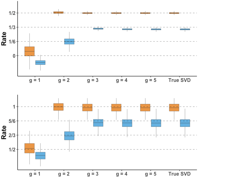
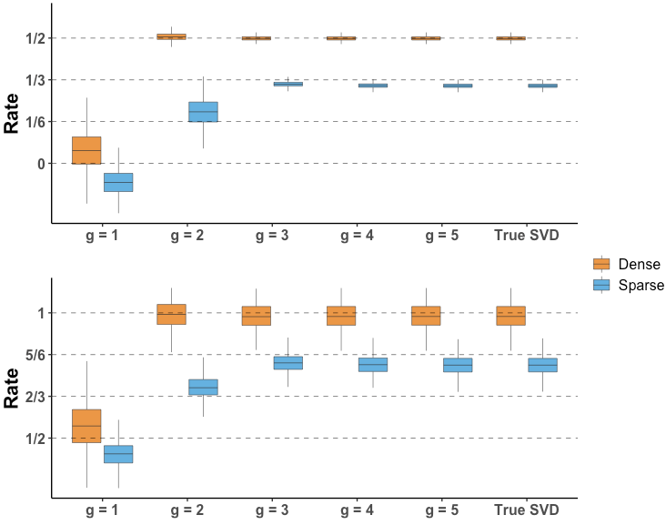
S.1.1.2 Exact recovery
We used the same simulation setting as that described in Section S.1.1.1 with and . For each combination of and for each , we generate an adjacency matrix with equal sized blocks and block probabilities . We then perform RSVD-based spectral clustering as described in Algorithm 2 with , where we use the Gmedian library in to perform fast (approximate) -medians clustering on the rows of . For comparison, we also use Gmedian to perform -medians clustering on the rows of . We repeat the above steps for Monte Carlo replicates. The proportion of times (among these replicates) in which the -medians clustering of either or correctly recover the community memberships for all nodes are reported in Table S.1 and Table S.2.
| Sparsity | OSC | |||||
|---|---|---|---|---|---|---|
| 1000 | 0.098 (0.013) | (0.000) | (0.000) | (0.000) | ||
| 2000 | 0.050 (0.010) | (0.000) | (0.000) | (0.000) | ||
| 3000 | 0.034 (0.008) | (0.000) | (0.000) | (0.000) | ||
| 4000 | 0.018 (0.006) | (0.000) | (0.000) | (0.000) | ||
| 5000 | 0.006 (0.003) | (0.000) | (0.000) | (0.000) | ||
| 1000 | 0.000 (0.000) | (0.012) | (0.000) | (0.000) | ||
| 2000 | 0.000 (0.000) | () | (0.000) | (0.000) | ||
| 3000 | 0.000 (0.000) | () | (0.000) | (0.000) | ||
| 4000 | 0.000 (0.000) | () | (0.000) | (0.000) | ||
| 5000 | 0.000 (0.000) | () | (0.000) | (0.000) | ||
| 1000 | 0.000 (0.000) | 0.000 (0.000) | (0.022) | (0.013) | ||
| 2000 | 0.000 (0.000) | 0.000 (0.000) | (0.021) | (0.005) | ||
| 3000 | 0.000 (0.000) | 0.000 (0.000) | (0.015) | (0.000) | ||
| 4000 | 0.000 (0.000) | 0.000 (0.000) | (0.009) | (0.000) | ||
| 5000 | 0.000 (0.000) | 0.000 (0.000) | (0.007) | (0.000) |
| Sparsity | OSC | |||||
|---|---|---|---|---|---|---|
| 1000 | 0.536 (0.022) | (0.000) | (0.000) | (0.000) | ||
| 2000 | 0.616 (0.022) | (0.000) | (0.000) | (0.000) | ||
| 3000 | 0.674 (0.021) | (0.000) | (0.000) | (0.000) | ||
| 4000 | 0.600 (0.022) | (0.000) | (0.000) | (0.000) | ||
| 5000 | 0.626 (0.022) | (0.000) | (0.000) | (0.000) | ||
| 1000 | 0.000 (0.000) | (0.012) | (0.000) | (0.000) | ||
| 2000 | 0.000 (0.000) | () | (0.000) | (0.000) | ||
| 3000 | 0.000 (0.000) | () | (0.000) | (0.000) | ||
| 4000 | 0.000 (0.000) | () | (0.000) | (0.000) | ||
| 5000 | 0.000 (0.000) | () | (0.000) | (0.000) | ||
| 1000 | 0.000 (0.000) | 0.000 (0.000) | (0.022) | (0.013) | ||
| 2000 | 0.000 (0.000) | 0.000 (0.000) | (0.014) | (0.000) | ||
| 3000 | 0.000 (0.000) | 0.000 (0.000) | (0.007) | (0.000) | ||
| 4000 | 0.000 (0.000) | 0.000 (0.000) | (0.003) | (0.000) | ||
| 5000 | 0.000 (0.000) | 0.000 (0.000) | (0.002) | (0.000) |
From Tables S.1 and S.2 we see that Algorithm 2 exactly recover the underlying community assignment with probabilities converging to as increases, provided that when and when . These empirical results are consistent with the theoretical results presented in Theorem 4.2, i.e., exact recover is guaranteed if and only if . Note that for , when and when . Finally we note that if and then RSVD-based spectral clustering occasionally recovers the community membership for all nodes. This is due to the fact that although with high probability, it does not prevent where is the minimum distance between any two nodes and belonging to different communities; exact recovery is certainly expected if .
S.1.1.3 Limiting distribution
We now illustrate the normal approximations for the row-wise fluctuations of , as implied by Theorem 3.4. For brevity we fixed and . Similar results are available for and . We generate a single realization of on vertices and , with equal sized blocks and block probabilities . Scatter plots of the rows of for as well as the rows of are presented in Figure S.2. From Figure S.2 we see that is sufficient for the rows of to be clustered into two clusters but is necessary for the empirical confidence ellipses of to match the theoretical confidence ellipses given in Theorem 3.4; the scatter plots for are also virtually indistinguishable from that for . In other words, the more stringent threshold in Theorem 3.4 is both necessary and sufficient for the normal approximations of ; note that for the current setting we have and hence .
Additional simulation results with respect to or , are further illustrated in Figures S.3–S.5. Since our theoretical results are valid up to some rotation, we shall orthogonally rotate the plots occasionally for the sake of better illustrations. Similar row-wise fluctuations and the corresponding phase transition phenomenon with respect to , can also been seen in these additional simulations.
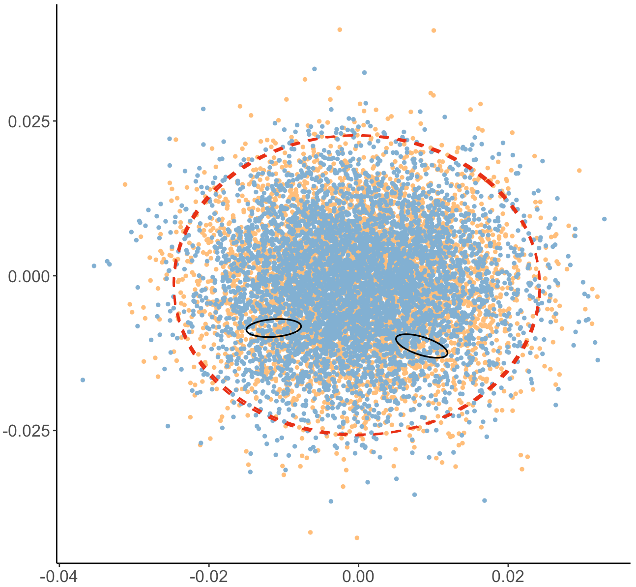
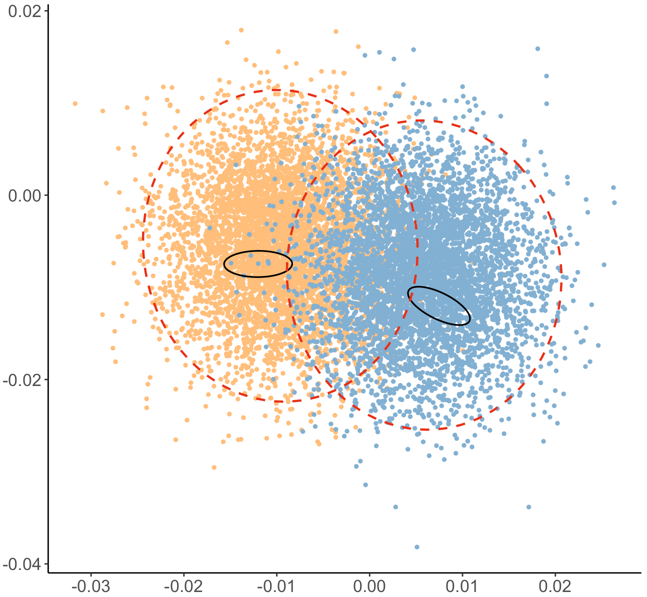
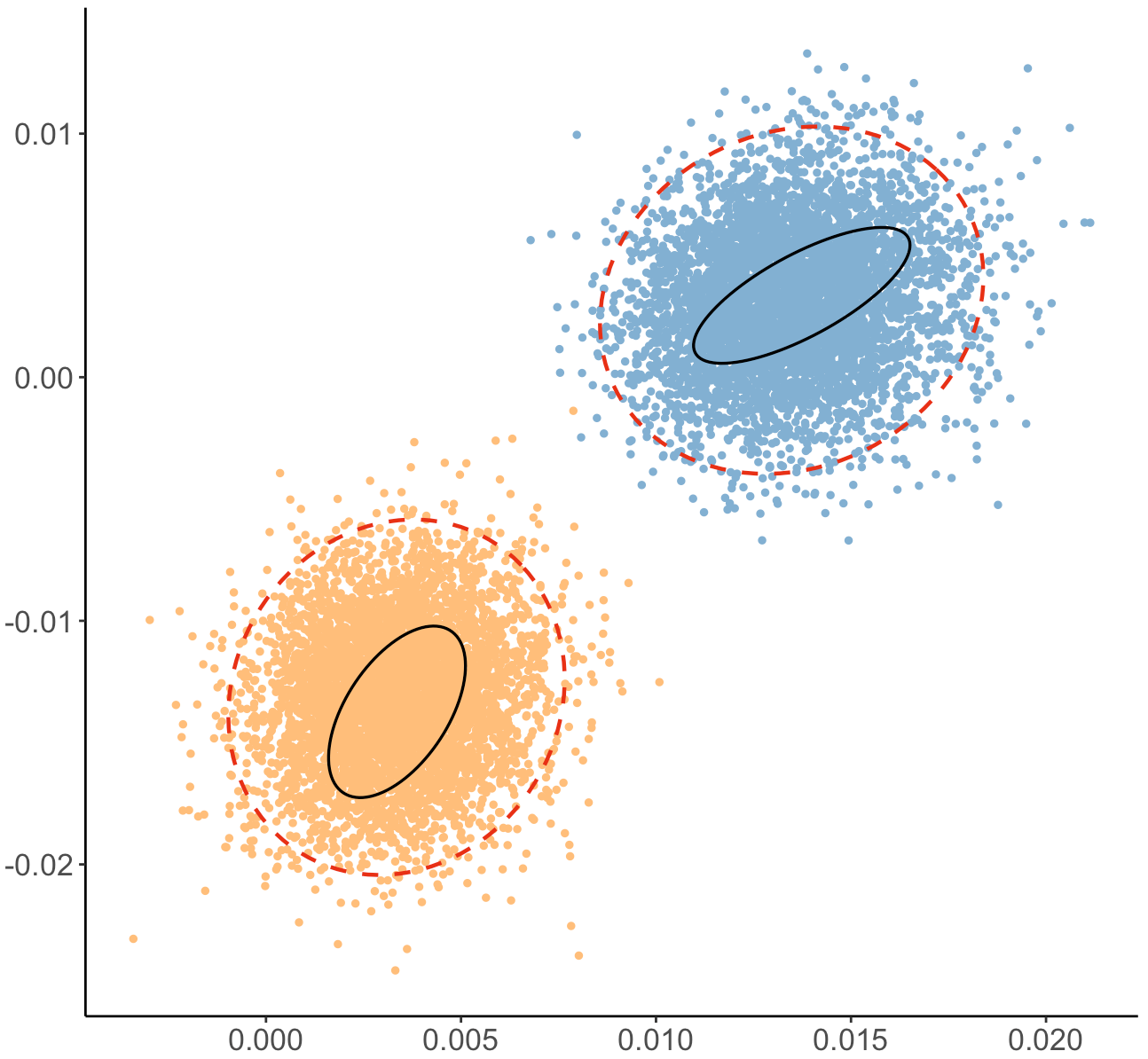

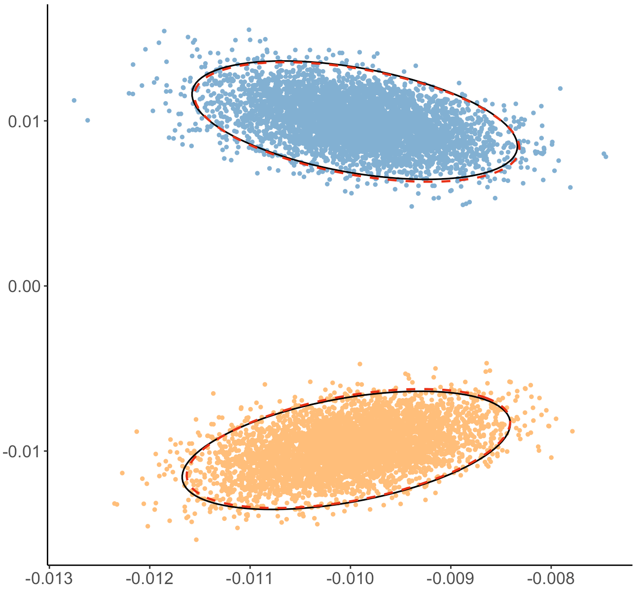
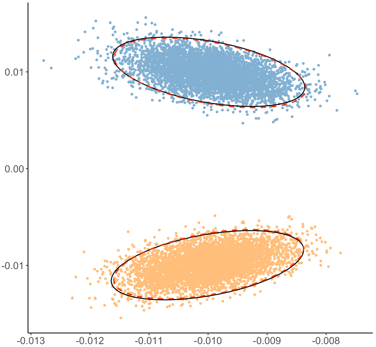
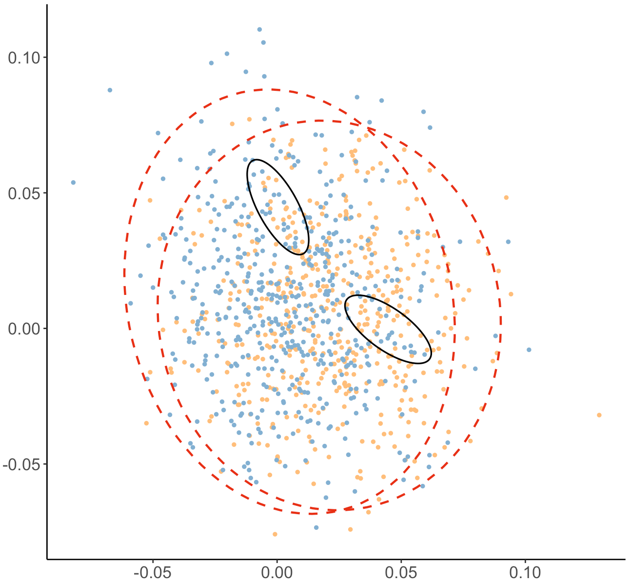
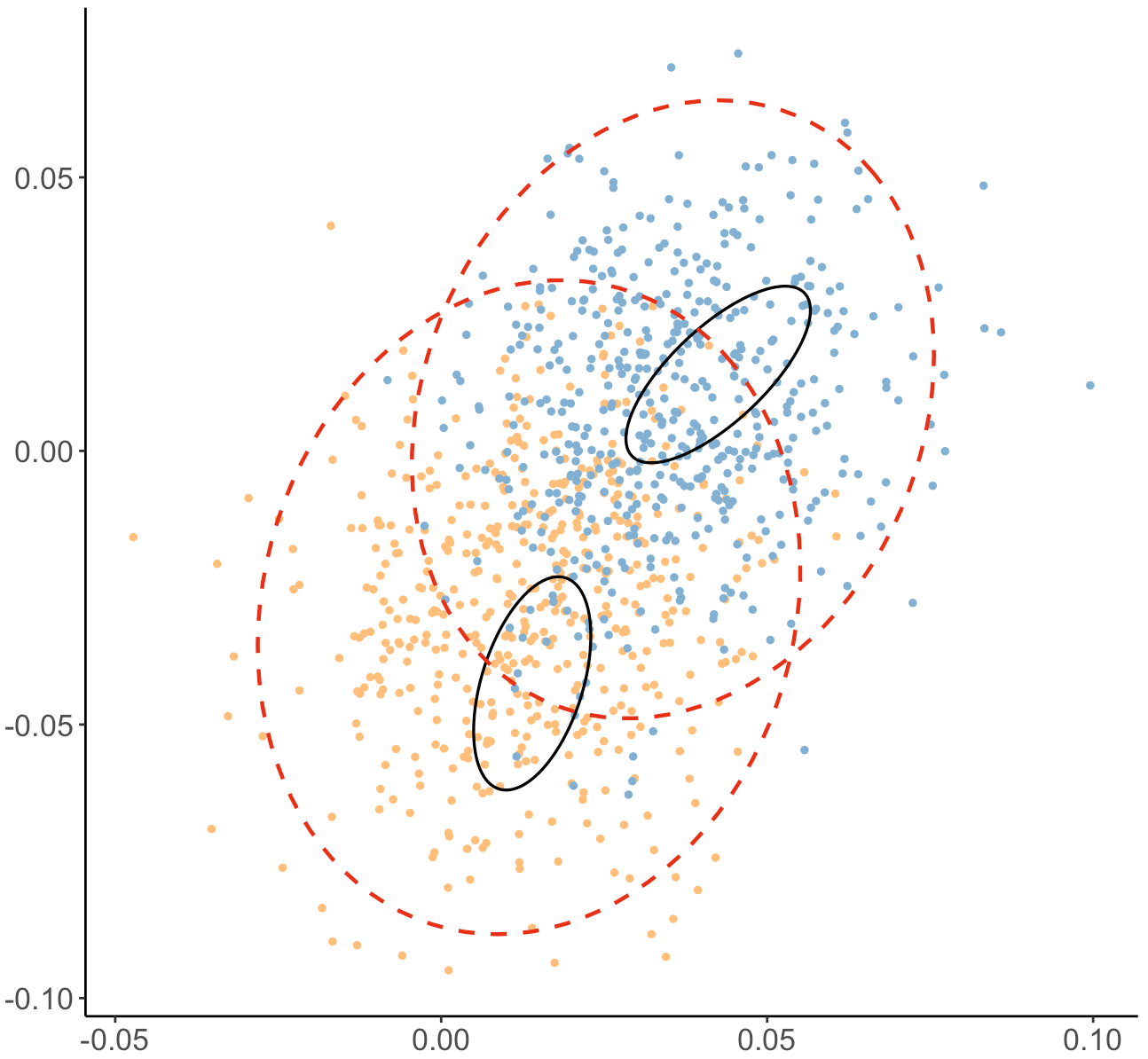
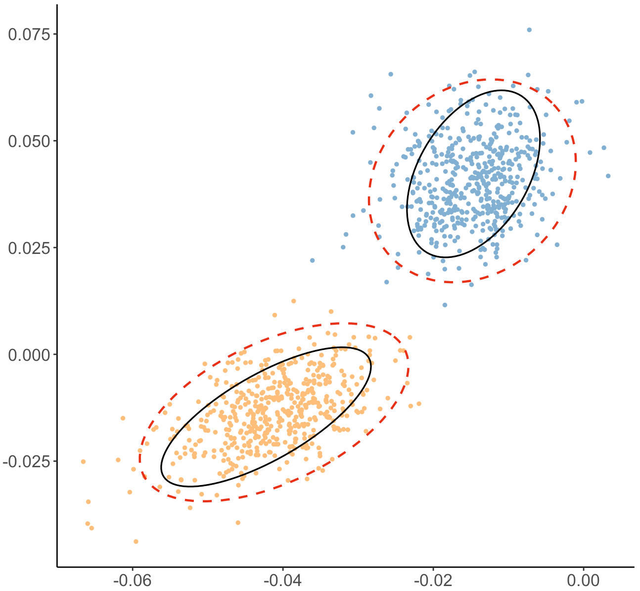
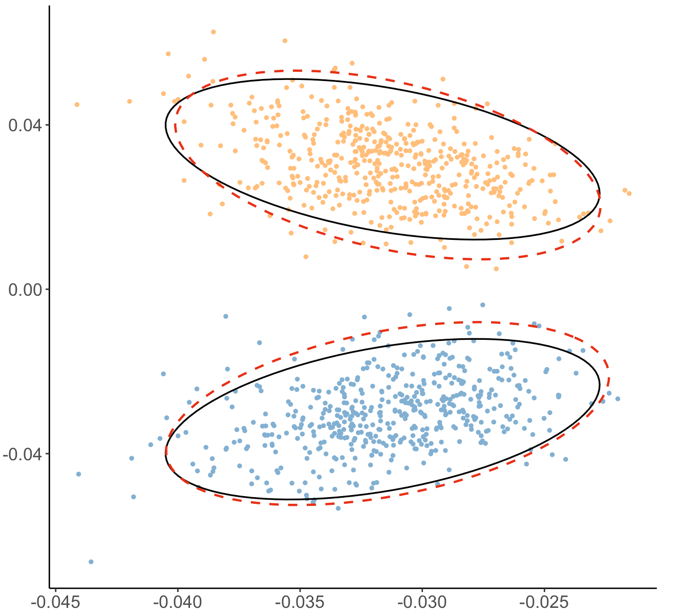
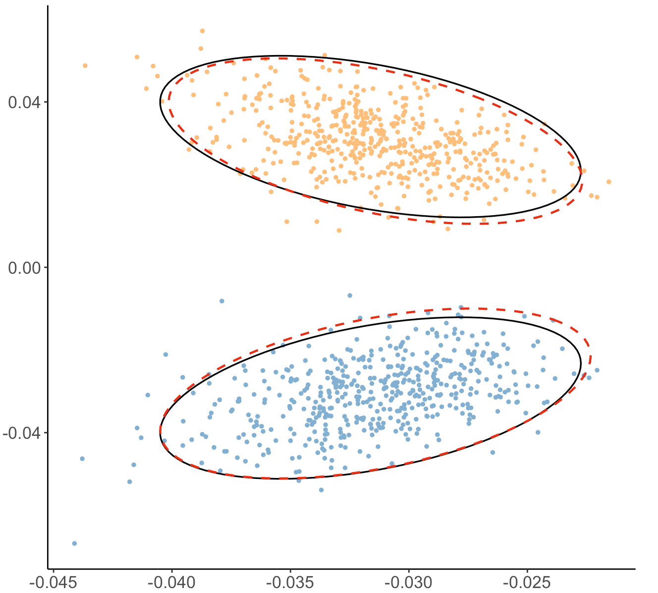
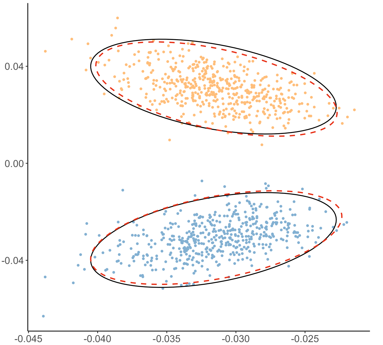
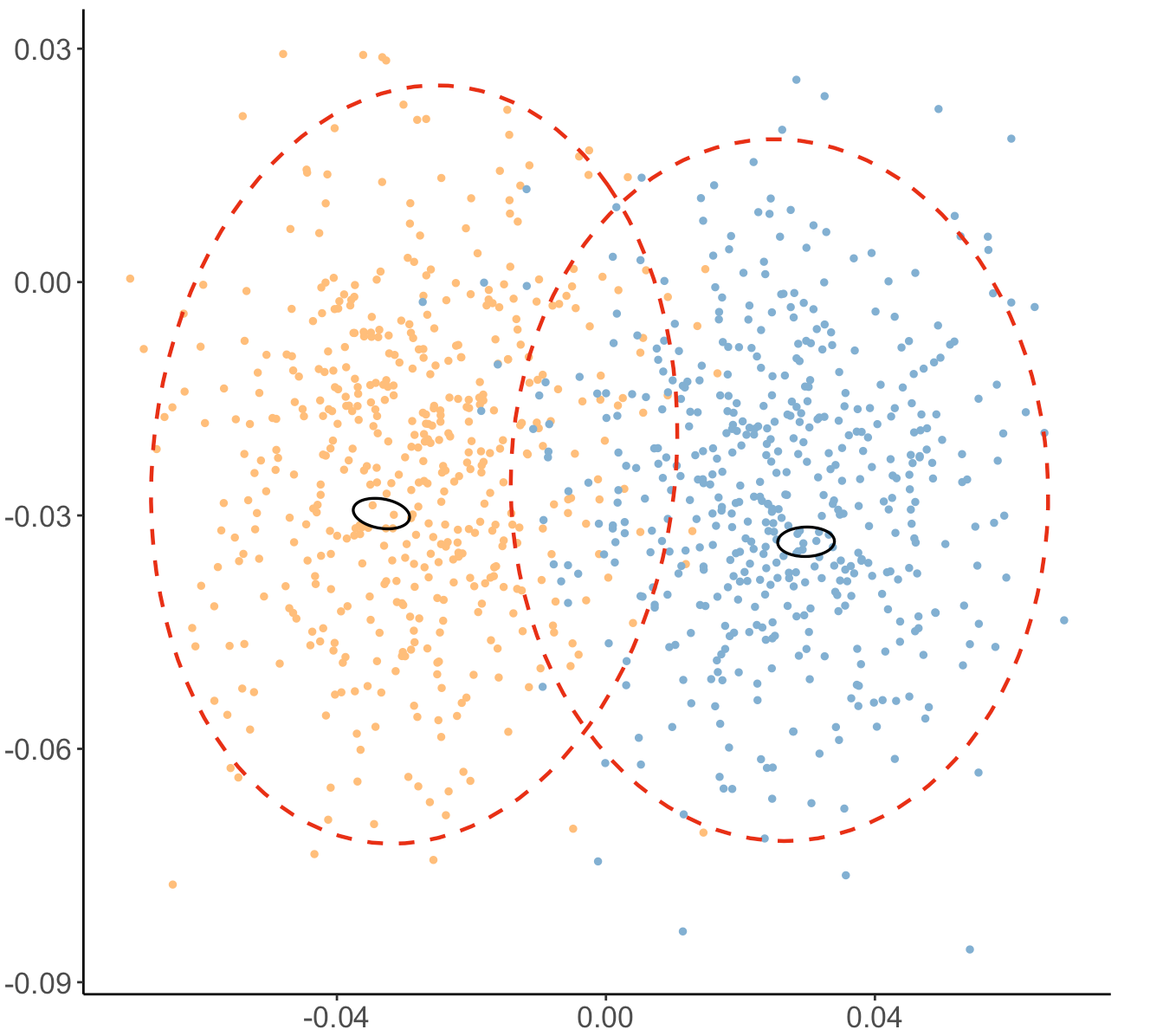
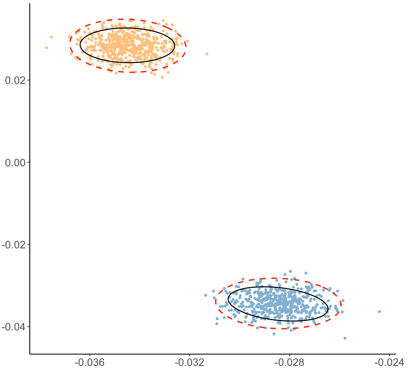
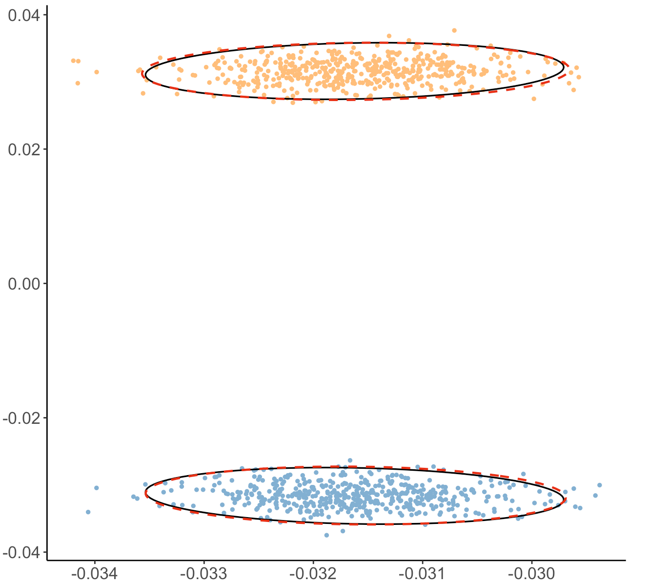
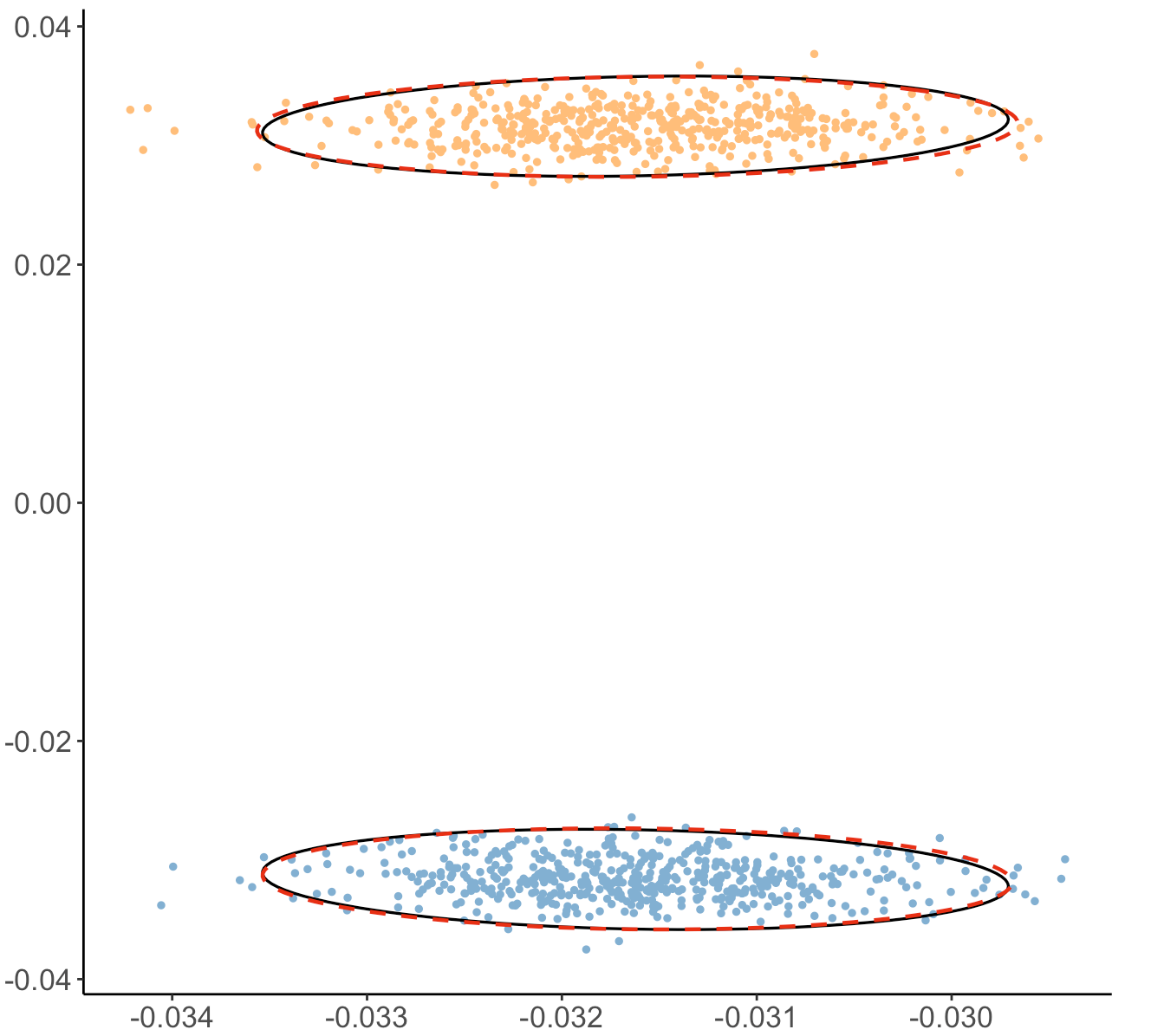

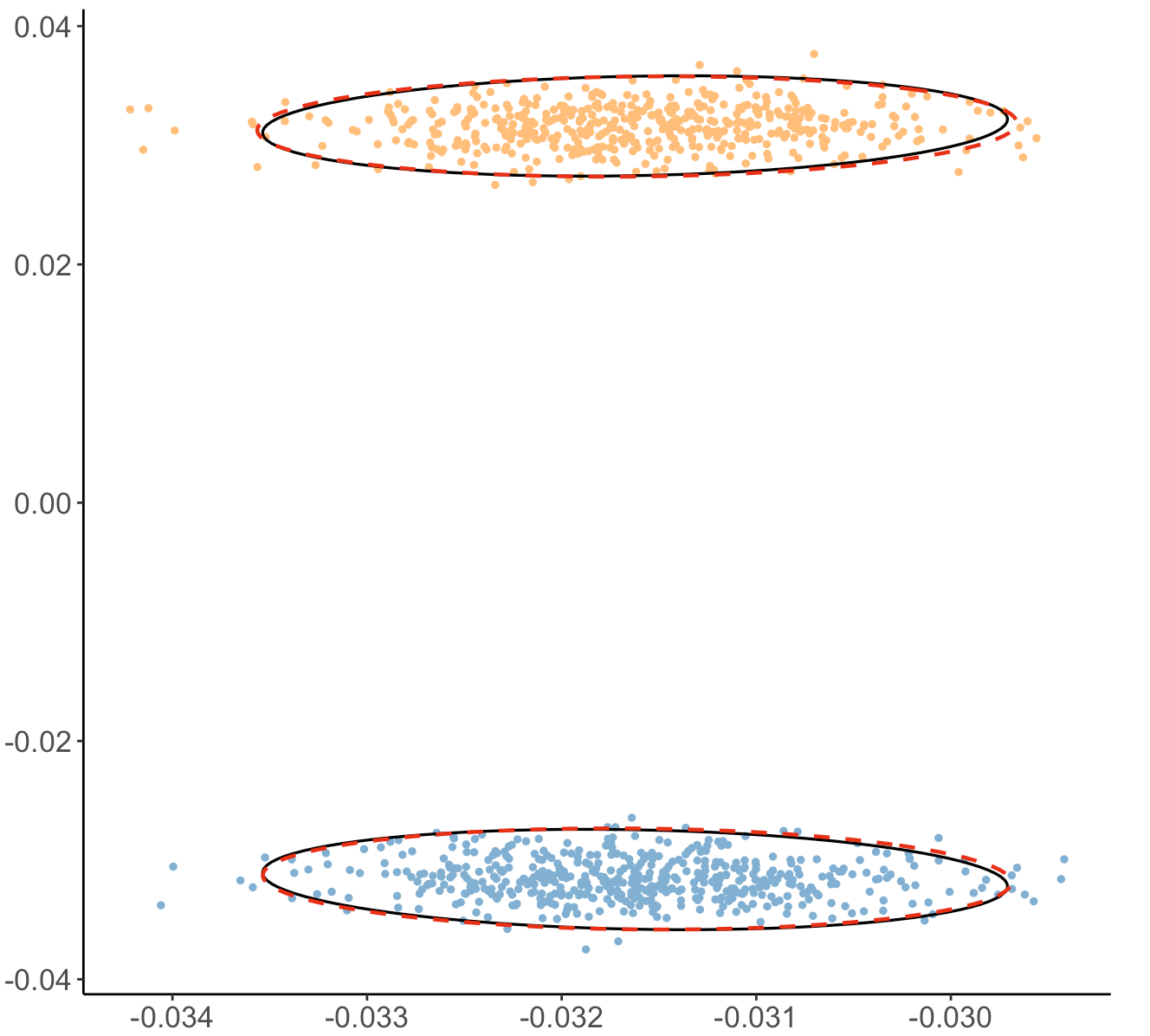
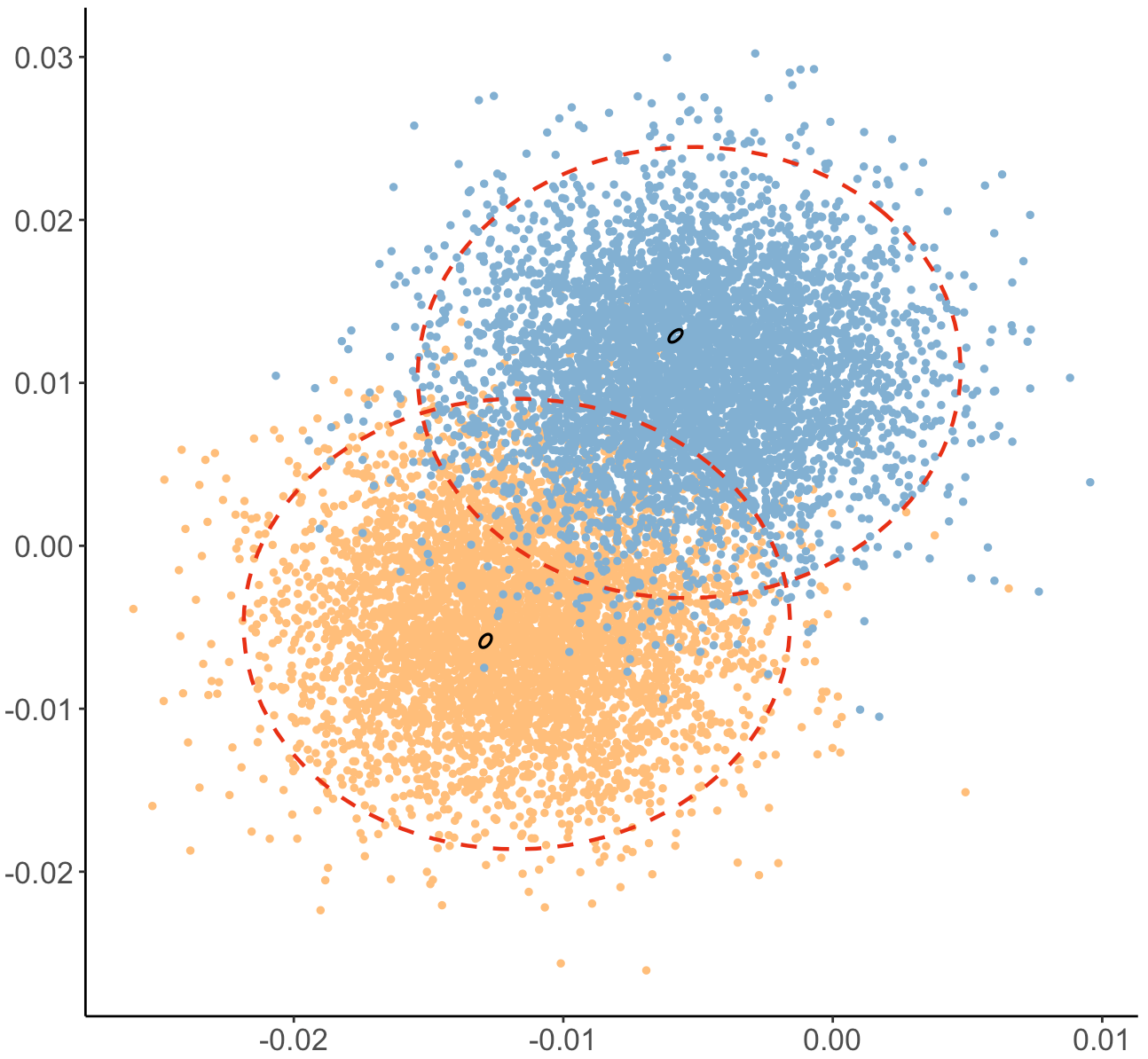
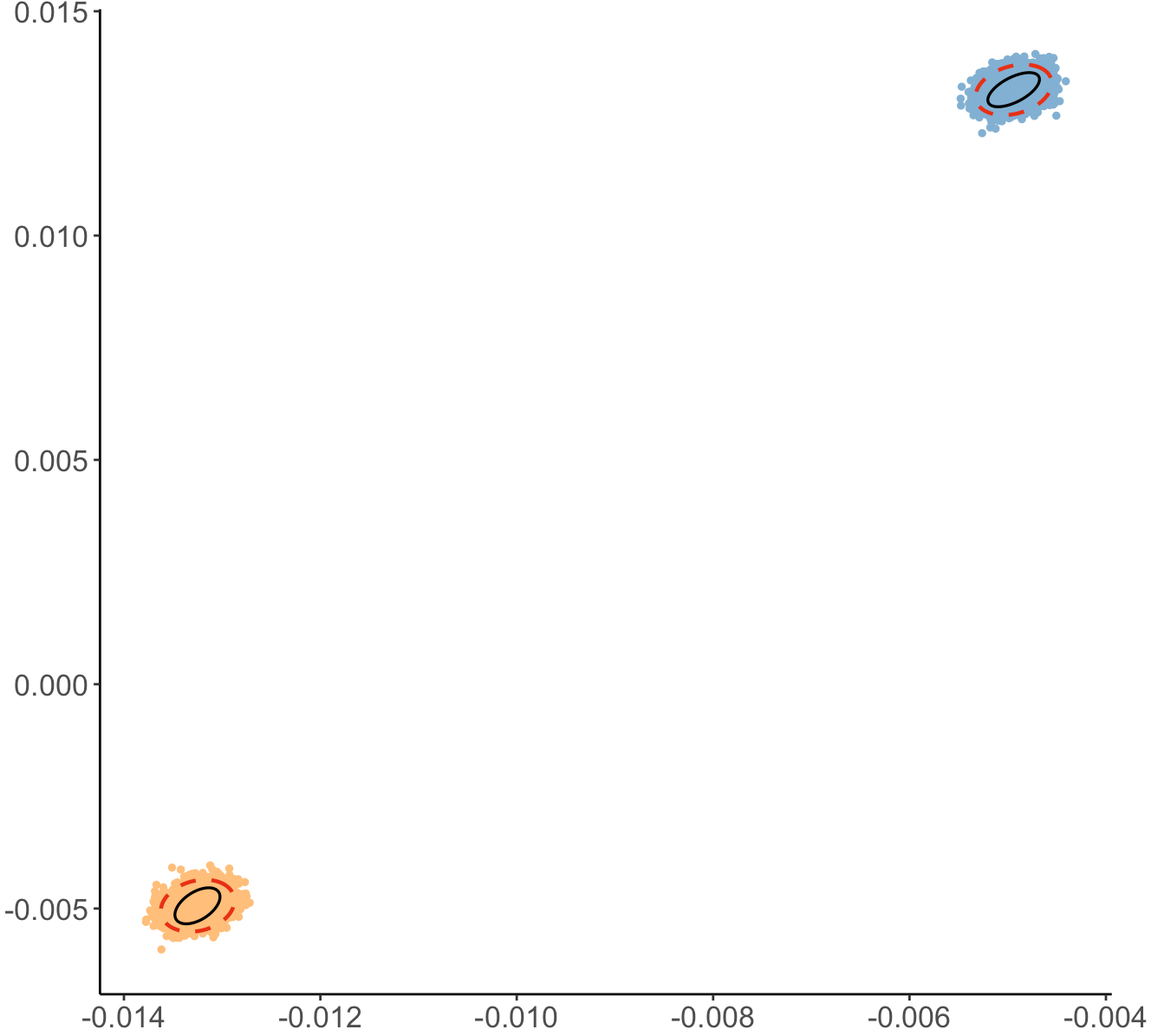
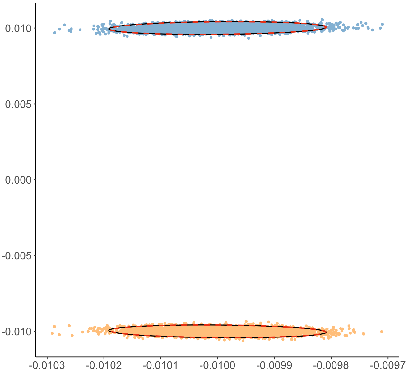


S.1.2 PCA with missing data
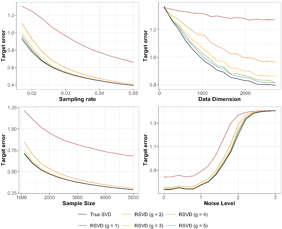
For this simulation study we used the same data generation mechanism as that described in section of [18] but with larger values of . More specifically we first sample a matrix whose columns are iid multivariate normal random vectors with mean and covariance matrix ; here is a matrix whose entries are iid standard normals. We then generate where the entries of are iid , the entries of are iid and denote the Hadamard product. The matrix represent a noisily observed version of (with missing entries).
Given we compute using Algorithm 4 with , , and . We then record ; here denote the matrix whose columns are the leading eigenvectors of . For comparison we also record where is the matrix of leading eigenvectors of and is as defined in Eq. (5.11).
Figure S.6 reports sample means for and as we vary the sampling probability , data dimension , sample size , and noise level ; these sample means are computed based on Monte Carlo replicates where we resampled the matrices and in each replicate. Figure S.6 shows that Algorithm 4 yields nearly-optimal performance (as compared to ) when for most settings of , , and . It is only when is large with respect to that have worse performance compared to and . Finally, is always sub-optimal. These observations are consistent with the theoretical results presented in Section 5.2.
S.1.3 Distance matrix completion
For this section we apply Algorithm 3 to recover the missing entries of a partially observed Euclidean distance matrix. In particular we use the world_cities dataset containing the locations of the most populous cities around the world; this dataset is part of the mdsr library in . We first construct the matrix whose elements are
Here and represent the longitude and latitude of the th city, respectively. We then sample a matrix (resp. by keeping roughly (resp. ) of the entries in , i.e., where is a symmetric matrix whose upper triangular entries are iid .
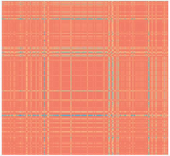
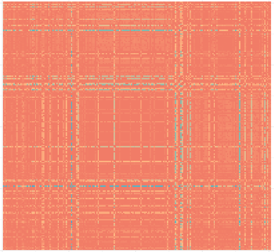
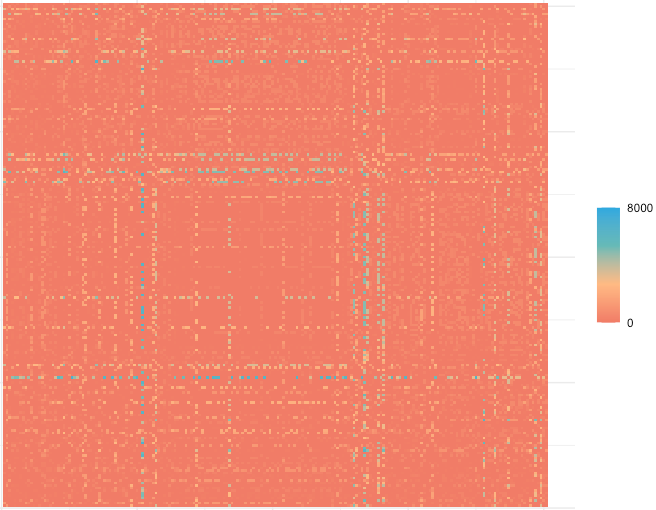
We now recover from (resp. ) using Algorithm 3. As the entries of are Euclidean distances between points in , we have . We therefore choose , and , and let (resp. ) be the resulting estimate of . For comparison we also consider the spectral estimate (resp. ) obtained by truncating the exact SVD of (resp. ); see [70] for more details.
A plot of the true distance matrix and one random realization of the partially observed and are presented in Figure S.7.The corresponding RSVD-based estimates and exact SVD based estimates of are then shown in Figure S.8–S.9. Figure S.8 shows that and both have comparable accuracy to while Figure S.9 shows that has much worse accuracy compared to and .
We also record the entrywise relative errors between the RSVD-based estimates (resp. the exact SVD-based estimate ) against that of . A summary of the quantile levels for these relative errors are presented in Tables S.3. The th–quantile of the entrywise relative errors between an estimate and the true distance is defined as the th quantile of ; for example the median relative error for and are and , respectively. Note that the numbers in Table S.3 are averaged over independent random samples of either or . From Table S.3 we see that the relative error decreases as increases with fixed; indeed, the relative error of is exactly the same as that for . Table S.3 also indicates that as decrease we need to increase to achieve a recovery rate close to that of . These observations are consistent with the theoretical results in Theorem 5.1.
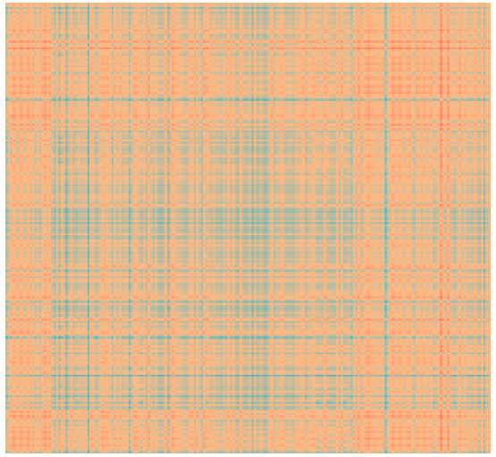
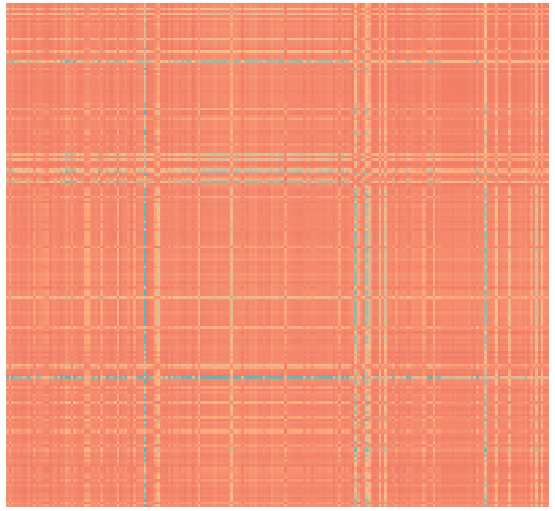
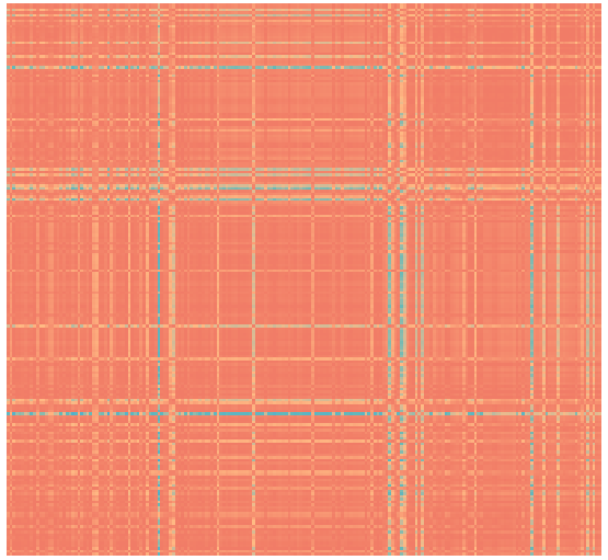
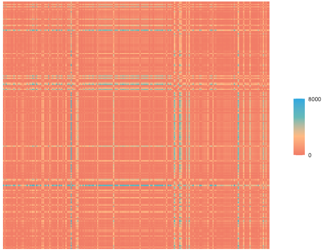
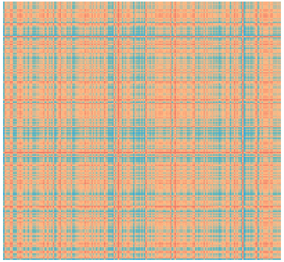
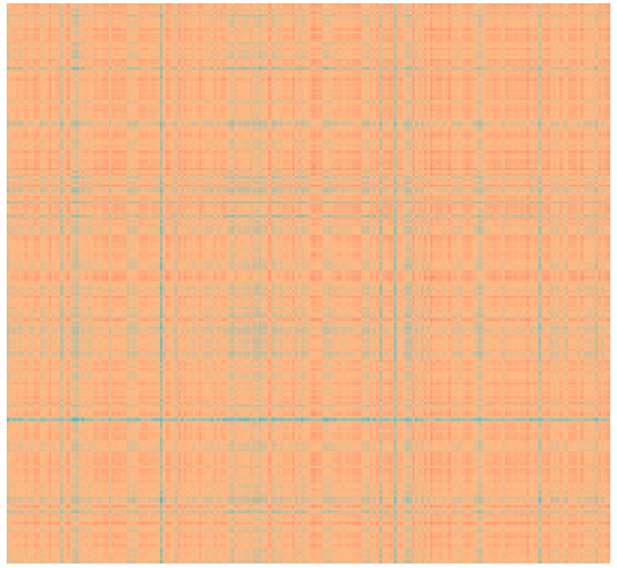
| 0.0169 (1.3) | 0.0515 (3.9) | 0.1315 (9.2) | 0.2203 (1.4) | 0.4232 (2.7) | 2.4408 (1.9) | 15.2389 (1.1) | ||
| 0.0035 (1.4) | 0.0107 (4.2) | 0.0273 (1.2) | 0.0453 (2.3) | 0.0789 (4.6) | 0.2798 (1.9) | 1.5766 (1.3) | ||
| 0.0024 (1.4) | 0.0073 (2.8) | 0.0182 (6.6) | 0.0289 (1.1) | 0.0464 (2.3) | 0.1531 (1.0) | 0.7823 (6.7) | ||
| 0.0024 | 0.0073 | 0.0182 | 0.0289 | 0.0464 | 0.1530 | 0.7816 | ||
| 0.0371 (3.6) | 0.1112 (1.0) | 0.2644 (2.1) | 0.4049 (2.7) | 0.6715 (3.0) | 3.8785 (2.0) | 24.4391 (1.4) | ||
| 0.0106 (3.7) | 0.0323 (1.2) | 0.0849 (3.5) | 0.1472 (7.2) | 0.2717 (1.5) | 1.3069 (1.0) | 8.9068 (7.0) | ||
| 0.0070 (9.6) | 0.0211 (3.0) | 0.0531 (8.2) | 0.0860 (1.5) | 0.1454 (3.4) | 0.5072 (1.2) | 3.0309 (9.8) | ||
| 0.0064 | 0.0194 | 0.0484 | 0.0774 | 0.1269 | 0.4439 | 2.4614 |
S.2 Extension to asymmetric matrices
We now extend Theorems 3.1–3.3 to the setting where and are either asymmetric or rectangular. Let be a matrix with and consider the additive perturbation where is a noise matrix. We once again assume that both and are unobserved, i.e., we only observed . Let and let denote the condition number of . Finally denote the SVD of as where is the diagonal matrix of non-zero singular values.
Given a matrix the rs-RSVD procedure for approximating the leading left singular vectors of is presented in Algorithm 5. The leading right singular vectors of can be approximated by considering and thus, without loss of generality, we will only focus on the left singular vectors of . Note that Algorithm 5 is equivalent to the PowerRangeFinder and SubspacePowerMethod procedures in [124, 58] when .
We now introduce a few assumptions on and ; these assumptions are natural generalizations of Assumptions 1– 2 for the symmetric case.
Assumption S.1 (Signal-to-noise ratio).
Let , , and . There exist fixed but arbitrary constants , and a quantity depend on , such that and
whenever . We view as the noise level of and as a lower bound on the SNR.
Assumption S.2.
S.2 There exists some positive constants such that, for any positive integer , any standard basis , and any given vector not dependent on , we have with probability at least that
when is sufficiently large. Here and when is even, and and otherwise. The is a finite constant not depending on and .
Remark S.2.1 (Divergence Regime).
In contrast to the symmetric matrix case, the quantities and now depend on both and and hence now depends on the growth rate of compared to . For an illustrative example, suppose that is a homogenous matrix whose entries are all of order and let be a standard Gaussian matrix. Assume also that for some constant . We then have and . Next suppose and are growing such that for some constant . We then have , , and .
Remark S.2.2 (Assumption S.2 Verification).
If the entries in are independent then we can verify Assumption S.2 by applying Proposition 3.2 together with a “symmetric dilation” argument. Consider, as an example, the case when is a standard Gaussian matrix as described in Remark S.2.1 with . Now define
Then is a symmetric matrix whose (upper triangular) entries are independent random variables satisfying the conditions in Proposition 3.2; see Example 2. We can therefore apply Proposition 3.2 to and show, for any standard basis , any vector and with even, that
with high probability. Bound for when is odd is derived similarly and hence satisfies Assumption S.2.
The following bounds for and for asymmetric follow mutatis mutandis from the proofs of Theorems 3.1–3.3 and the conditions posited in Assumptions S.1 and S.2; see Section S.6.6 for a sketch of the arguments. We surmise that normal approximations for the row-wise fluctuations of are also available in the asymmetric setting and we leave the precise formulation of this result and its conditions to the interested reader.
Theorem S.2.1.
Suppose Assumption S.1 holds, and that is computed using Algorithm 5 with satisfying one of the three conditions (a)–(c) as specified in Theorem 3.2. Assume also that . Denote . Let and where is a constant not depending on . We then have the following bounds.
-
(Spectral-norm Concentration):
With probability at least ,
(S.2.1) -
( Perturbation):
With probability at least ,
(S.2.2) - ( Perturbation):
Note that the parameter in Algorithm 5 and Theorem S.2.1 actually represents power iterations of . We show in Section 4 that, in the context of random graphs inference, doing or power iterations is often sufficient for to converge to in both and distances. This is consistent with the recommendation of or provided in [58, Section 1.6].
S.3 General theoretical results for any
We first state a set of slightly more general versions of Theorem 3.1, Theorem 3.2, and Theorem 3.3. More specifically the following results provide bounds for and conditional on , i.e., the resulting bounds depend on several quantities associated with such as . Given these results, we derive Theorem 3.1 through Theorem 3.3 by bounding the quantities that depend on separately through a set of technical lemmas. In particular Lemma S.4.4 and Lemma S.4.5 provide these bounds for the case where is chosen via repeated sampling of independent Gaussian matrices as described in Algorithm 1 of this paper. We note that this type of approach allow us to easily extend our results to other class of sketching matrices. Indeed, suppose is a random Rademacher matrix or a random column-subsampling matrix. Then Theorem 3.1 through Theorem 3.3 will continue to hold for this choice of provided that we can establish analogous results to that of Lemma S.4.4 and Lemma S.4.5.
Theorem S.3.1.
Let where and satisfy Assumption 1. Let be a fixed but arbitrary integer and let be any matrix. For let be the matrix whose columns are the right singular vectors of and define
| (S.3.1) |
Then for sufficiently large , we have with probability at least that
| (S.3.2) |
The bound for in Theorem S.3.1 together with the Wedin Theorem [122] implies the following bound for and .
Theorem S.3.2.
Assume the setting in Theorem S.3.1. Then for sufficiently large , we have with probability at least that
| (S.3.3) |
S.4 Technical lemmas
Before commencing with the proofs of the main results, we first state some technical lemmas that we will repeatedly use throughout this paper. We start by listing some basic properties of the norm.
Lemma S.4.1.
For any and , we have
For a proof of Lemma S.4.1, see e.g., [22]. The next two results, namely Lemma S.4.2 and Lemma S.4.3, will be used for bounding in Theorem 3.1.
Lemma S.4.2 (Decomposition of powered matrices difference).
Let and be two square matrices. Denote . Then for any integer we have the expansion
Proof of Lemma S.4.2.
Let . We then have the expansion
| (S.4.1) | ||||
If then we can repeat the above step for and obtain
In summary, by iterating the expansion in Eq. (S.4.1) a total of times, we derive
as desired. ∎
Lemma S.4.3.
Proof of Lemma S.4.3.
By definition, we have
Next, by Assumptions 1, we have , with probability at least as . We now bound . Since is a matrix, let us denote the SVD of by
where is a matrix, is a diagonal matrix, and is a matrix. Once again by Assumption 1 we have
| (S.4.2) |
with probability at least . Note the above upper bounds only relies on the high probability bound of , with probability at least , and thus they hold simultaneously with probability at least . ∎
The following Lemma S.4.4 and Lemma S.4.5 provide a collection of bounds for the quantities depending on in the statement of Theorem S.3.1 through Theorem LABEL:thm2:res, when is chosen via repeated sampling of independent Gaussian matrices as described in Algorithm 1.
Lemma S.4.4.
Proof of Lemma S.4.4.
In the following argument we always condition on and . As the final bounds for and does not depend on the choice of and , we can then uncondition with respect to and to obtain the desired results.
We first bound . We have
where is th entry of . Since is standard Gaussian, there exists a universal constant such that for all ; see e.g Section 2.5.1 of [120]. Let be arbitrary. Then by the union bound, we have
| (S.4.3) | ||||
Note that the last inequality follows from .
We next bound . Recall the non-asymptotic bound for the spectral norm of a Gaussian random matrix (see e.g. Corollary 5.35 in [119]). Then for a standard Gaussian matrix and , we have
| (S.4.4) |
with probability at least . As each is a matrix with iid standard Gaussian entries, we can set , and in Eq. (S.4.4) to obtain with probability at least . A union bound over all yields
| (S.4.5) |
We finally bound . Recall that in Algorithm 1 the are generated independently of the and . Hence, conditional on , the and , for and , are standard Gaussian matrices. Recall also that . By Eq. (S.4.4), we therefore have with probability at least . The same bound also holds for . Now choose . We then have, by a union bound over and , that when is sufficiently large,
where the last inequality follows from the fact that . ∎
Lemma S.4.5.
Suppose Assumption 1 hold, and is generated via Algorithm 1 with where and satisfy either one of the three following conditions
-
(a).
Both and are fixed.
-
(b).
is fixed and is growing with .
-
(c).
is growing with and for some fixed .
Now choose for some sufficiently large but fixed constant ; a detailed discussion for the value of is given in Remark 3.3. Assume also that the condition number satisfies . Let be fixed but arbitrary. Then with probability at least , we have
Proof of Lemma S.4.5.
We recall the notations in Eq. (LABEL:decom:M:hatM). For any we have
| (S.4.6) |
Now is positive semi-definitive and hence, by Weyl’s inequality,
| (S.4.7) |
From the description of Algorithm 1 we have
| (S.4.8) |
We now show that the term on the right-hand side of the above display can be lower-bounded by a term of the form .
As is positive semi-definitive for all , we have
Note that, by Assumption 1 and Weyl’s inequality, we have
with probability at least . Recall that we had assumed in the statement of Lemma S.4.5. Thus is negligible compared to when increases. We therefore have
| (S.4.9) |
with probability at least .
Thus, to obtain a lower bound for in Eq. (S.4.8), we only need to lower bound in Eq.(S.4). Let be a random matrix whose entries are independent standard normal random variables and let be the cumulative distribution function (CDF) for the smallest singular value of , i.e., define
| (S.4.10) |
for all . We first condition on an observed . Then for any , the matrix is identically distributed as and furthermore the collection of matrices are mutually independent. Thus, by the definition of , we have
for any arbitrary . As the probability on the right-hand side above does not depend on the particular choice of , we can now uncondition on to obtain
Combining Eq.(S.4.9) and Eq. (S.4) we have
| (S.4.11) |
with probability at least .
We now consider three scenarios, namely (a) and are both fixed, (b) is fixed and is growing with and (c) and are both growing with .
Case (a). Suppose both and are fixed. Then for any arbitrary there exists a finite such that (see e.g. Section 4.4 in [43]); we emphasize that depends on , and but does not depend on . There thus exists a constant depending only on such that if then . Set . Then by Eq. (S.4.11), we have with probability at least .
Case (b). Suppose is fixed and is growing with . Then by the non-asymptotic bound of a “tall” Gaussian matrix [37] we have
| (S.4.12) |
Now let and for some sufficiently large but finite . As is fixed, Eq. (S.4.11) implies
| (S.4.13) |
with probability at least
Note that the second to last inequality in the above display follows from Eq. (S.4.12), provided that . Let . Then for we have that Eq. (S.4.13) holds with probability at least .
Case (c). Suppose for some . Let for some . Then by Eq. (S.4.12), we have
| (S.4.14) |
Note that as . Let . We then have
| (S.4.15) |
Combining Eq. (S.4.11), Eq. (S.4.12), Eq. (S.4.14), and Eq. (S.4.15), we obtain
| (S.4.16) |
with probability at least , provided that for some finite . We emphasize that depends only on such that decreases when increases.
Summarizing the results for the above three cases considered in Lemma S.4.5, we have that if then
| (S.4.17) |
with probability at least . We therefore have
with probability at least . Finally the above derivations also show that (a) depends only on and if and are both fixed, (b) can be any constant larger than , and (c) depends only on when both and are growing. ∎
The last technical lemma is used when bounding in Theorem 3.3.
Lemma S.4.6.
Let where and satisfy Assumption 2. Let be any arbitrary matrix not depending on . Let be fixed but arbitrary. Then for sufficiently large , we have with probability at least , that simultaneously
where is some constant dependent only on .
Proof of Lemma S.4.6.
Under Assumption 2, a similar argument to the section 3.5 of [22] yields
| (S.4.18) | ||||
with probability at least . Here denote the th standard basis in and is the th column vector of . The same argument also yields
| (S.4.19) | ||||
with probability at least . Here is the th column of .
Finally we bound . We start with the expansions
| (S.4.20) | ||||
We will bound the norm for each individual term in the right hand side of the above display. By Eq. (S.4.18), we have
| (S.4.21) |
with probability at least .
Now let . We then have, with probability at least ,
| (S.4.22) | ||||
where the first inequality in the above display follows from Lemma S.4.1 and the last two inequalities follow from Lemma S.4.3 and .
Next suppose . Then using Eq. (S.4.18) we have, with probability at least ,
| (S.4.23) | ||||
for any . Recall that under Assumption 1, we have for some . We therefore have
for any . In other words, the bound in Eq. (S.4.23) when is dominated by that when . Collecting the bounds in Eq.(S.4.21), Eq. (S.4.22) and Eq. (S.4.23), we obtain
| (S.4.24) | ||||
with probability at least with some large enough yet fixed when is fixed. Note that we had used Assumption 1 to bound as increases. The desired results follow immediately by unifying Eq. (S.4.18), Eq. (S.4.19), and Eq. (S.4.24). ∎
S.5 Proofs for Section 3
S.5.1 Proof of Theorem S.3.1
If then, by Assumption 1, we have
with probability at least . We next consider . Let . Using the expansion for in Lemma S.4.2, we have
| (S.5.1) |
We now bound the spectral norms of each of the terms through .
Bounding By Assumption 1 we have, with probability at least ,
| (S.5.2) |
Bounding By the triangle inequality we have
| (S.5.3) |
First suppose that . Then with probability at least , we have
| (S.5.4) | ||||
where the last inequality follows from Lemma S.4.3 and Assumption 1.
Plugging the bounds from Eq. (S.5.4) and Eq. (S.5.5) into Eq. (S.5.3) yield
| (S.5.6) |
with probability at least . Here we had used the fact that is fixed and that dominates for all as .
S.5.2 Proof of Theorem S.3.2
We note that is an additive perturbation of , i.e.,
Since is rank , we have that is also rank and hence . Let and be the matrix of left and right singular vectors of , respectively. We thus have, by Wedin’s - theorem [122], that
| (S.5.8) | ||||
with probability at least . Note that the last equality follows from the bound for in Theorem S.3.1.
S.5.3 Proof of Theorem S.3.3
We denote by and the solution to the Frobenius-norm Procrustes problems
| (S.5.9) |
We note that the convergence rate of is equivalent to the convergence rate of since, by Proposition 3.1, almost surely. Furthermore, from the definition of , we have .
We will thus focus our effort on bounding . Let . Taking in Theorem 3.1 of [22], we have the decomposition
| (S.5.10) | ||||
Note that if then since as . We now bound the norms of the three terms (or four terms when ) on the right-hand side of Eq. (S.5.10).
Bounding . We have, with probability at least , that,
| (S.5.11) | ||||
Here the last inequality uses the bound for given in Theorem S.3.1 together with the fact that for some almost surely (see Proposition 3.1) and thus .
We now consider . If then by Lemma S.4.6 we have
with probability at least . For we first recall the expansion given in Eq. (S.5.1). We now bound through .
Bound for . By Lemma S.4.6 we have, with probability at least , that
| (S.5.12) |
Bound for . Using the expansion in Eq. (S.5.3) and Eq. (S.5.4), we have
| (S.5.13) | ||||
Recall the bound for given in Lemma S.4.3. Let . We then have, with probability at least ,
| (S.5.14) | ||||
where the penultimate inequality in the above display follows from Lemma S.4.6.
Bound for . From Lemma S.4.3 we have, with probability at least ,
| (S.5.15) | ||||
Combining the above bounds for , and , we obtain
| (S.5.16) | ||||
with probability at least . Recalling Eq. (S.5.11), we conclude that
| (S.5.17) |
with probability at least .
Bounding . We have, with probability at least , that
| (S.5.18) | ||||
Note that the last inequality in the above display follows from Theorem S.3.2 and Eq. (S.5.16) while the bound is given in Lemma 6.8 of [22]. Finally we had used the fact that ; see the discussion after Eq. (S.5.11).
Bounding : Recall Eq. (LABEL:decom:MgG). We immediately have,
| (S.5.19) | ||||
S.5.4 Proof of Theorem 3.1
We prove Theorem 3.1 by combining Theorem S.3.1 and Lemma S.4.4. More specifically, by Theorem S.3.1 we have
| (S.5.21) |
with probability at least , where is chosen among independent standard Gaussian matrices according to Algorithm 1. Substituting the bounds for and from Lemma S.4.4 into Eq. (S.5.21) we obtain
| (S.5.22) |
with probability at least when is sufficiently large. The first part of Theorem 3.1 is thus established.
S.5.5 Proof of Theorem 3.2
We prove Theorem 3.2 by combining Theorem 3.1, Theorem S.3.2 and Lemma S.4.5. More specifically, by Theorem S.3.2 we have
| (S.5.24) |
with probability at least . Recall that we assumed in the statement of Theorem 3.2. Lemma S.4.5 then implies
| (S.5.25) |
with probability at least . Now when , Eq. (3.3) in Theorem 3.1 implies,
| (S.5.26) |
with probability at least when . Substituting Eq. (S.5.25) and Eq. (S.5.26) into Eq. (S.5.24) yields the desired result. Note when , Eq. (3.2) and Eq. (S.5.25) similarly yields a weaker bound in Eq. (3.5). ∎
S.5.6 Proof of Corollary 3.1
S.5.7 Proof of Theorem 3.3
Let . Now define the quantities
| (S.5.27) | |||
| (S.5.28) |
Recall Theorem 3.2, Theorem S.3.3, and the error bounds in Lemma S.4.4 and Lemma S.4.5. In particular, with probability at least , we have simultaneously,
We therefore have, with probability at least ,
Hence, by Theorem S.3.3, we have
| (S.5.29) |
with probability at least ,
Now consider . Recalling Eq. (S.5.23), we have
| (S.5.30) |
For , recall that for some . We then have
We therefore have
| (S.5.31) |
where if either or , and otherwise.
S.5.8 Proof of Corollary 3.2
We only consider the case where as
Recall Proposition 3.1. Let and where and through are the matrices appearing in Eq. (S.5.10). We then have
| (S.5.33) | ||||
We now bound the max norm of the four terms on the right-hand side of Eq. (S.5.33). Recall that from the proofs of Theorem S.3.3 and Theorem 3.3 we have
with probability at least . We now bound and . Our bounds for these quantities depend on bounds for , etc., given in Theorem 3.1, Theorem 3.2 and Lemma S.4.4 through Lemma S.4.6. For conciseness we generally omit specific references to these bounds in the following derivations.
Bounding . Using the expressions for through given in the proof of Theorem S.3.3, we have (recall that )
with probability at least .
Bounding . We first bound where and the are as given in Eq. (S.5.1).
-
•
Similar to Eq. (S.5.12), with probability at least , we have
- •
- •
-
•
Similar to Eq. (S.5.15), with probability at least , we have
Combining the above bounds we have
| (S.5.35) |
with probability at least ; here is a poly-log factor.
Using the above bounds for in spectral and norms, we obtain
with probability at least . In the above derivations, we had used the assumption that which converges to faster than any poly-logarithmic factor in .
Given the above bounds for and , we are now ready to bound the max norm of each term in the right-hand side of Eq. (S.5.33). We will frequently use the inequality .
- 1.
-
2.
Bounding . Note that . We then have, with probability at least ,
and thus .
-
3.
Bounding . Note that . We then have, with probability at least ,
and thus .
-
4.
Bounding . Decompose . Then with probability at least
and thus .
Combining the above results yield as desired. ∎
S.5.9 Proof of Theorem 3.4
We first make a few remarks. For ease of presentation, and as Theorem 3.4 is a limit result, we say that an event happens with high probability (whp) if happens with probability at least . Here is a finite constant that can change from line to line. In addition, the conditions assumed in Theorem 3.4 are at least as restrictive as those assumed in Theorems 3.1 through Theorem 3.3 and Lemmas S.4.4 through Lemma S.4.6. and hence the error bounds provided in Theorems 3.1 through Theorem 3.3 and Lemmas S.4.4 through Lemma S.4.6 still hold whp. For example, when and we have by Eq. (S.5.30) and Eq. (S.5.31) that, whp,
| (S.5.36) | ||||
where the constant is specified in Assumption 2.
Our main proof strategy is as follows. First, we derive an upper bound for the norm of . In particular we show that the row-wise fluctuations of is negligible compared to the row-wise fluctuations for . The row-wise limiting distributions of are thus the same as those for . The proof is then completed by invoking limiting distribution for in Assumption 3.
We now bound . Let . Recalling Eq. (S.5.10), we have
| (S.5.37) |
where and by Proposition 3.1. Then by Eq. (S.5.18) we have, whp,
Similarly by Eq. (S.5.20) we have, whp,
We further decompose the term in Eq. (S.5.37) as follows. By splitting the second term in the expansion for given in Lemma S.4.2’s, we have
| (S.5.38) | ||||
Let . Reordering the terms in Eq. (S.5.38), we obtain
Note that in the above derivations we had used the fact that, by the definition of in Eq. (LABEL:decom:M:hatM), we have for all . We now show that, ignoring logarithm terms, and can be bounded by whp.
Bounding . The following claim provides a high-probability bound for . For ease of exposition we defer its proof to Section S.7.16
Claim S.1.
Assume the setting of Theorem 3.4, we have whp,
Bounding. For , by Lemma S.4.1, we have
| (S.5.39) | ||||
For the first term on the right-hand side of Eq. (S.5.39), we have whp
| (S.5.40) | ||||
by Lemma S.4.6, where we define
| (S.5.41) |
and the second inequality is by , , and . For the second term in Eq. (S.5.39), we have whp
| (S.5.42) | ||||
where the second inequality is by Lemmas S.4.3 and S.4.5, the third inequality is from the bound whp by Lemma S.4.4, and the last inequality is because and . As , combining Eq. (S.5.40) and Eq. (S.5.42) yields, whp,
Summarizing the above results, we have
Now for any , we have . Recall that is the singular value decomposition of and furthermore, for some orthogonal matrix . We therefore have
Substituting the above relationship into Eq.(S.5.9), we obtain
| (S.5.43) |
We now bound and .
Bounding . We first state the following claim whose proof, for ease of exposition, is deferred to Section S.7.4.
Claim S.2.
Assume the setting of Theorem 3.2 where and is fixed. We then have whp,
Let . By Claim S.2 we have
| (S.5.44) | ||||
whp, where the second inequality in the above display is by Lemma S.4.1 while the third inequality is by Assumption 1, Lemma S.4.5, and Claim S.2.
Bounding . By definition, we have, whp,
| (S.5.45) | ||||
Let . As , we have from the above bounds for that
| (S.5.46) | ||||
in probability, where the final convergence in Eq. (S.5.46) follows from Eq. (3.14). Here is given in Eq. (3.15) and is an upper bound for logarithmic factors appearing in through . Recalling Eq. (S.5.43) and the relationship , we obtain
Therefore, by Slutsky’s theorem, we have
as . Indeed, by Eq. (S.5.46), is negligible in the limit while the convergence of to is by Assumption 3. Note since and are exactly equal, by the rotation invariant of Frobenius norm, we actually have , where solves Procrustes problem between and such that
| (S.5.47) |
∎
S.6 Proofs for Section 4, Section 5, and Section S.2
S.6.1 Proof of Theorem 4.1
Recall that and is the left singular matrix of . For this proof we define a sparsity scaling parameter such that and . By Lemma S.4.5, is invertible with probability at least . Now suppose that is invertible. Then and hence
Let and . We then have,
| (S.6.1) | ||||
In the above derivations we used the fact for any matrices and whose products and are well defined, and the relationship . Next note that
which together with Eq. (S.6.1) yields
| (S.6.2) | ||||
Let . We then have the identity
Define the quantities
We now bound through .
Bounding . Write the SVD of as where and . As and are independent, there exists a constant such that, with probability at least ,
| (S.6.3) |
See the proof of Lemma S.4.4 for a derivation of the above bound. We thus have, with probability at least ,
where the last inequality in the above display used the following claim whose proof can be derived using the expansion for given in Lemma S.4.2 together with the high probability bound for from Assumption 1.
Claim S.3.
Assume the setting of Theorem 4.1. Choose a fixed . Then with probability at least we have .
Now , , and . Therefore by Lemma S.4.5 we have, with probability at least ,
We therefore have, with probability at least ,
Bounding and . Recall the proof of Theorem S.3.1, in particular the bounds for and in Eq. (S.5.6) and Eq. (S.5.7). Now and hence
| (S.6.4) |
with probability at least . We therefore have
with probability at least . Next let be the matrix whose columns are the left singular vectors of . We then have, by Claim S.3 and Eq. (S.6.4),
with probability at least . Note that we had bound with probability at least similar to Eq. (S.6.3). Collecting the above bounds for through and recalling Eq.(S.6.2), we obtain
| (S.6.5) |
where with probability at least .
Our last step is to lower bound . As and are both positive semi-definite matrices, we have
where is the th column of .
Now by Theorem 3.1, Lemma S.4.4, and Assumption 1, we have
| (S.6.6) | ||||
with probability at least . Recall that for are iid standard Gaussian matrices. By the spectral norm bound of a standard Gaussian matrix [45], we have
| (S.6.7) |
with probability at least where is some large but finite constant. Together with Eq. (S.6.6), we have with probability approaching ,
| (S.6.8) |
noting here is negligible as for some .
In summary, with probability approaching , we have
| (S.6.9) |
We now bound . Let be an arbitrary constant and let be a finite constant such that . The existence of follows from the assumption and Markov’s inequality. Next define the event
where and are constants not depending on . Assumption 1 implies that occurs with probability approaching . Now suppose that occurs. and let be an -dimensional standard Gaussian random vector that is independent of . We then have
| (S.6.10) |
where the above expectations are with respect to and conditional on .
Now fix an and a . As is a random vector whose elements are iid standard normal independent of , the Hanson-Wright inequality for quadratic forms [61] implies
for any ; here and are constants not depending on . We thus have, by a union bound over all and ,
Recall that is fixed and . We now choose for some sufficiently large . Then, with high probability (assuming occurs)
| (S.6.11) |
where the last inequality follows from Eq. (S.6.10). As occurs with probability approaching , we can now uncondition with respect to and still have the bound in Eq. (S.6.11) holding with probability approaching .
In summary, combining Eq. (S.6.5), Eq. (S.6.9) and Eq. (S.6.11), we have with probability approaching that
Note that for the above derivations if then
and therefore is negligible, while if then dominates which makes the first term ; thus is also negligible. The lower bound for is thereby established. The lower bound for follows immediately from the lower bound for and the relationship . ∎
S.6.2 Proof of Theorem 4.2
Let and . We will verify that these matrices satisfy Assumption 2. Let be the number of nodes in the th community. By the law of large numbers, we have for all that,
| (S.6.12) |
almost surely as . We now define the normalized membership matrix
and let . Without loss of generality, e.g., by reordering the rows and columns of so that the first vertices are assigned to community , the next vertices are assigned to community , and so on, can be represented as
By Eq. (S.6.12) and an elementwise argument, almost surely, where . Weyl’s inequality then implies
where . Now is a fixed matrix not depending on and for all . As is an orthogonal matrix, we have
Therefore with , and , asymptotically almost surely. Next by the definition of we have with . Hence, by Theorem 5.2 in [76], there exist a constant such that, with probability at least ,
| (S.6.13) |
Assumption 1 therefore holds with and . Furthermore by Proposition 3.2 we have that satisfies Assumption 2. See Example 1 for more details.
Given Assumptions 1–2, and with satisfying the conditions in Theorem 3.3, we have that if then
| (S.6.14) |
with probability at least . Here and are as defined in Eq. (S.5.27) and Eq. (S.5.28). It is well-known that the coherence is bounded: a.s. (see e.g. the proof of Theorem 5.2 in [75]). Therefore, since , , and , we have
which, when combined with Eq. (S.6.14), yields
| (S.6.15) |
with probability at least . Eq. (S.6.15) implies that, with high probability, the distance between the th and th rows of when is always smaller then the distance when . Hence, clustering the rows of using either the -means or -medians algorithm will exactly recover with probability at least . See for example Theorem 2.6 in [82] and Theorem 5.2 in [75] for proofs of this claim for -means and -medians, respectively. ∎
S.6.3 Proof of Theorem 5.1
S.6.3.1 Preliminary
Let and . Now define , and accordingly. We have two choices for , namely, and . Since for any norm , we choose and bound in Frobenius norm and max-norm. Finally we also derive the entrywise limiting distribution for .
S.6.3.2 Assumption verification
We first verify that and satisfy Assumption 1. As has bounded condition number, we have . Next write
| (S.6.16) |
Now is a random symmetric matrix whose upper triangular entries are independent mean random variables with
Furthermore we also have
| (S.6.17) | ||||
By Remark 3.13 in [11], there exists a universal constant such that for ,
which immediately implies, with probability at least . On the other hand, with probability at least , see e.g., Lemma 13 in [3]. Eq. (S.6.16) therefore implies
| (S.6.18) |
with probability at least . We can thus choose for some finite constant . In summary we have
| (S.6.19) |
where the last inequality follows from the assumption in Eq. (5.2).
We next verify Assumption 2. Recall Proposition 3.2. Now let and
Note that we require in the statement of Proposition 3.2 and this is satisfied when for some arbitrary constant as assumed in Eq. (5.2). We then have,
| (S.6.20) | ||||
where , and are defined as follows
We now bound the two terms on the right-hand side of Eq. (S.6.20).
-
•
Let . Each entry of takes on two distinct values and are uniformly bounded from above by . There thus exists some constant such that
for all . See Example 1 for more details.
-
•
Now where is symmetric with iid upper triangular entries and the random sampling is independent of . We therefore have
Recall Example 2 and note that . There thus exists a constant such that for any we have
where we had defined and .
In summary if then
for all ; here is a finite constant. As , satisfies all conditions in Proposition 3.2 and hence also satisfies Assumption 2.
S.6.3.3 Bounding and
S.6.3.4 Bounding
Recall that we defined . Now by Eq. (S.6.18), Eq. (S.6.19), and the assumption (as has bounded condition number), we have with probability at least that
| (S.6.22) |
We now bound for some fixed . As we have
| (S.6.23) |
Since , we have and . Eq. (S.6.21) and Eq. (S.6.22) therefore imply
with probability at least . Similarly, by Eq. (S.6.18),
with probability at least . Combining the above results with Eq. (S.6.23) we obtain
with probability at least .
S.6.3.5 Bounding
S.6.3.6 Entrywise limiting distribution and confidence interval
Fix a . We will derive the limiting distribution of for any where ; the same result also holds for . For ease of exposition we say that an event happens with high probability (whp) if happens with probability at least . Here is a an arbitrary constant that can change from line to line.
Compared with the entrywise concentration bound in Eq. (S.6.24), the entrywise limiting distribution requires substantially more detailed analysis. For clarity we first state a general entrywise CLT result which does not depend on the matrix completion setting and then apply this result to derive the normal approximations in Eq. (5.5) and Eq. (5.7).
Theorem S.6.1.
Suppose Assumptions 1–2 hold with fixed and bounded . Let be generated via Algorithm 1 with , where the universal constant is given in Remark 3.3, and . Define the random variable,
where is defined in Theorem 3.4. Fix an and suppose that there exists a quantity depending possibly on such that
Then, provided that in probability, we also have
The proof of Theorem S.6.1 is deferred to Section S.6.5. To apply Theorem S.6.1, we first derive an upper bound for (see Claim S.4). We next compute where is obtained by truncating the entries of . Using this we show that and in probability. Theorem S.6.1 then implies . Finally we show that the quantities and defined in Eq.(5.6) satisfy and in probability. Our derivation of the limiting distribution for follows the same ideas as that presented in [28] but our derivations are for the RSVD estimates while the derivations in [28] are for . Nevertheless, for completeness we will present most of the technical details with references to [28] when appropriate.
Before getting into the proof note that by Eq. (5.2) we have
| (S.6.25) | |||
| (S.6.26) |
where both of the above convergence are in probability.
We first consider a truncated version of . Recall where . Let and let be the matrix whose entries are the . Now define
| (S.6.27) |
Now by the tail bounds for Gaussian distribution, we have
See [28, Section 3.2.3] for more details. We thus have and whp. The following result uses to bound ; see Section S.7.6 for a proof.
Claim S.4.
Assume the setting of Theorem 5.1. We then have whp that
Claim S.4 implies
whp and hence in probability. Recalling the definition of in Theorem S.6.1 we obtain
| (S.6.28) | ||||
with high probability.
Let be the variance of . We first bound from below using a similar argument to the proof of Theorem 4.12 in [28]. Using this bound we then show that is negligible whp. Denote and note that
for all . Following the proof of Lemma 4.19 in [28] we have
| (S.6.29) | ||||
As the distribution of is symmetric around , the distribution of is also symmetric around and . We therefore have
| (S.6.30) | ||||
provided that is sufficiently large. The inequality in the above display is derived as follows. Let . By the Cauchy–Schwarz inequality we have
| (S.6.31) |
and hence
Under the conditions of Theorem 5.1 we have that is bounded away from and , and thus
| (S.6.32) |
We therefore have, by Eq. (S.6.28), that
| (S.6.33) | ||||
We now show that in probability. As and , we have and thus
Also, since is homogeneous, the are homogeneous. As and have bounded condition number, the are also homogeneous, i.e., and hence
| (S.6.34) |
Combining Eq.(S.6.33), Eq. (S.6.34), and Eq. (S.6.25), and recalling the assumption for some constant , (see (5.2)) we conclude that in probability.
Now we show the limiting distribution of . Write
The summands on the right-hand side of the above display are independent mean random variables. Similar to the proof of Lemma 4.19 in [28], we invoke the Berry–Esseen Theorem to show the desired limiting distribution. We first check the third-order moment condition for , i.e.,
in probability. Note that the penultimate inequality in the above derivations follows from Eq. (S.6.32) and the bound
| (S.6.35) |
with high probability, and the last inequality follows from Eq. (S.6.34) and Eq. (S.6.25).
Let be the CDF of and denote . Then by the Berry–Esseen bound (see e.g. Theorem 4.21 in [28]), we have
as . Now whenever and hence
as . In summary we have . Recall that in probability and hence, by Theorem S.6.1, we have
| (S.6.36) |
We next show that in probability and hence can be replaced by in without changing the limit result in Eq.(S.6.36); here is defined in (5.4). Recall that and hence
Then, by Eq. (S.6.30) and Eq. (S.6.31), we have
and thus
| (S.6.37) |
Now recall the definitions of and . Then by Eq. (S.6.32) and Eq. (S.6.37), we have
where the last equality is because ; see Eq. (S.6.30). In summary we have in probability, as desired.
We now derive the confidence interval for given in Eq. (5.7). This is equivalent to showing that in probability where is defined in Eq. (5.6). We first define
Using the same argument as that for deriving Eq. (4.171) in [28], we have
| (S.6.38) | ||||
with high probability. We now bound . Recall that we had defined in the statement of Theorem 5.1. Now let where is defined in Eq. (S.6.27) and let
Then whp and . As whp, we have by Eq. (S.6.24) that
whp. Now recall Eq. (S.6.34) and Eq. (S.6.35). We then have
whp. Furthermore, we have by Eq. (S.6.21) that
whp and hence
whp. In summary we have whp that
We can now use the same arguments as that presented in Eq. (4.176)–Eq. (4.177) of [28], but with terms depending on replaced by terms depending on . More specifically let . We then have, after some straightforward but tedious algebra, that
| (S.6.39) | ||||
whp. In particular the last inequality in the above display is derived as follows.
-
(i)
Let . Then
whp. Note that we had used the fact that in the above derivations.
- (ii)
-
(iii)
Finally let . Then
whp where we had used the fact that .
Note that and are upper bounds for the terms denoted by and in Eq. (4.176) and Eq. (4.177) of [28], respectively. Combining Eq. (S.6.29), Eq. (S.6.38), and Eq. (S.6.39), we have whp that
where the last equality is by Eq. (S.6.34) and Eq. (S.6.26). In summary we have in probability and hence, by Slutsky’s Theorem and Eq. (S.6.36), we have
as desired.
S.6.4 Proof of Theorem 5.2
The proof uses the same ideas as that presented in the proof of Theorem 3.3 and thus, for conciseness, we only sketch some of the main steps here. Define . Then with probability at least , we have
| (S.6.40) |
and conditional on given , with probability at least ,
See Section 8.2 and Section 10.2 in the supplementary material of [18] for derivations of these bounds. Then we can condition on a high-probability event such that given satisfying for all . Recall that we have assumed bounded condition number among . So we then take and in Assumption 1 with bounded and for some fixed constant . By (S.6.40), we further have . Then by Theorem 3.2 and the fact that is independent with and , we can uncondition the high-probability event of , and the desired results follow immediately.∎
S.6.5 Proof of Theorem S.6.1
We first recall the decomposition of in Eq. (S.5.43), i.e.,
| (S.6.41) |
where are defined in the proof of Theorem S.3.3 in Section S.5.3, and , are defined in the proof of Theorem 3.4 in Section S.5.9; in particular solves the orthogonal Procrustes problem between and (see Eq. (S.5.47)). We emphasize that Eq. (S.6.41) holds for general matrices and , and does not require Assumption 3 and Eq.(3.14) to be satisfied. For this proof we only consider and note that the same arguments also apply when . For ease of exposition we say that an event happens with high probability (whp) if happens with probability at least where is a finite constant that can change from line to line.
Let and note that . Then from Eq. (S.6.41) we have
| (S.6.42) | ||||
The following claim provides upper bound for , and ; we deferred its proof to Section S.7.7. As is orthogonal, the same bounds also hold for and .
Claim S.5.
Recall that
We now bound the max norm of each term on the right-hand side of Eq. (S.6.42) by . We will repeatedly use the observations that (1) for some and thus decreases to faster than any factor and (2) .
-
1.
. As and thus
Each of the above terms are less than and hence whp.
-
2.
. We decompose . First we have
Furthermore we have
In summary, we have whp.
-
3.
. We have whp,
-
4.
. We have . First, we have
whp. Second, we have whp,
In summary, we have whp.
-
5.
. We decompose . First we have
whp. Second we have whp
In summary, we have whp.
-
6.
. We decompose . First we have
Second we have
whp. In summary we have whp.
-
7.
. We decompose . First we have
whp. Second we have whp
In summary we have whp.
-
8.
. We decompose . First whp
Second we have whp,
In summary we have whp.
Substituting the above bounds into Eq. (S.6.42) we have, for any , that
where whp. Then, under the condition of Theorem S.6.1, we have
by Slutsky’s theorem. ∎
S.6.6 Proof of Theorem S.2.1
Theorem S.2.1 follows mutatis mutandis from the proofs of Theorem 3.2 and Theorem 3.3, with the conditions in Assumptions 1 and 2 replaced by those in Assumptions S.1 and S.2. For brevity we only present proof sketches for the bounds and given in Eq. (S.2.1) and Eq. (S.2.2). The bound for in Eq.(S.2.3) is also straightforward but requires more tedious book-keeping and is thus omitted.
Let be the left singular vectors of where is matrix whose enties are iid standard normals. As almost surely, is equivalent to , i.e.,
| (S.6.44) |
almost surely. See also the proof of Proposition 3.1 in Section S.7.1.
We now introduce some notations. Let be any positive integer and be arbitrary matrices of dimensions . First define
where if is even and otherwise. Next, for , define
Finally, define
We say that an event happens with probability at least if where is some fixed constant not depending on .
We now derive the bound for given in Eq. (S.2.1). Similar to Lemma S.4.2, we have
Bounding : Similar to Eq. (S.5.2), we have with probability at least ,
Then similar to Eq. (S.4.4) and Eq. (S.4.5), we have
with probability at least . In summary, with probability at least .
Bounding : First we note that
We now bound . Suppose that is odd (the case when is even follows the same identical argument). We then have
Then, similar to Eq. (S.5.3), we have,
with probability at least . Similar to Lemma S.4.3, let be the right singular vectors of . We then have
| (S.6.45) | ||||
with probability at least . Therefore, with probability at least ,
and thus .
Bounding : Once again we focus on the case where is odd. First note that
Next, similar to Eq. (S.5.7) and Eq. (S.6.45), we have
| (S.6.46) | ||||
with probability at least . In summary, similar to Eq. (S.5.7), we have
with probability at least .
Combining the upper bounds above for , and we obtain
with probability at least , where . Now recall Assumption S.1. Then by choosing , we have
| (S.6.47) |
with probability at least . Eq. (S.2.1) is thereby established.
Bounding : Denote the SVD of as
where is the diagonal matrix formed by the largest singular values of and is the diagonal matrix for the remaining singular values. Similar to Eq. (S.4.6)– Eq. (S.4), we have for any that
Therefore, by Weyl’s inequality,
When , similar to Eq. (S.4), we have with probability at least . Next, using the same arguments as that for deriving Eq. (S.4)–Eq. (S.4.17), we obtain
with probability at least , provided that and satisfy one of the conditions (a)–(c) as specified in Theorem 3.2 and for some universal constant . In summary we have, with probability at least ,
| (S.6.48) |
S.7 Additional Proofs
S.7.1 Proof of Proposition 3.1
When , we have by Eq. (LABEL:decom:M:hatM). Then where is a diagonal matrix with full rank. In addition, since is chosen from many standard Gaussian matrix with , and , it is easy to see each is a standard Gaussian matrix. Recall that .
Now if has rank then is matrix with rank and thus, as a result, the column space of coincides with the column space of . As is the left singular matrix of and , there exists an orthogonal such that . By the definition of for , we have
| (S.7.1) |
Finally, since for any (see e.g. [44]) and is chosen from , we immediately have . Therefore, we conclude that Eq. (S.7.1) holds almost surely.∎
S.7.2 Proof of Proposition 3.2
The ideas of this proof are adapted from the proof of Lemmas 6.5 and 7.10 in [48]. We first assume that is entrywise independent and then extend it to the case where is symmetric with independent (upper-triangular) entries. Fix a particular basis vector and a vector not depending on . Our target event can be written as
| (S.7.2) |
where and . We now derive an upper bound for . Denote, for brevity, .
Case a. () When , we have
By the moment conditions of , we know for any ,
| (S.7.3) |
In addition, are independent mean zero random variables. Then, by taking in Lemma 3.8 in [48], we have when is fixed,
with probability at least , provided that . Here is a constant depending only on , and the divergence rate of , while is a constant depending only on . Eq. (S.7.3) can be rewritten as which implies the desired result.
Case b. () We first note the following two deterministic bounds: By the moment condition of , we have when ,
for any . Next, if and is sufficiently large such that and , then
In other words, there exists a constant (henceforth ) depending only on , and the divergence rate of such that for all , for any , and for all we have
| (S.7.4) |
We next introduce some additional notation. Let denote a generic pair with . The th coordinate of (with ) is denoted as . For two pairs and , define .
We now bound the th moment of for integer . By definition, we have
| (S.7.5) | ||||
where denote a collection of integers (not necessarily distinct) from , , and denote a collection of pairs (not necessarily distinct) from . For brevity we use to denote a generic and . Then, for any ,
| (S.7.6) |
where now runs over all possible combinations of . For a particular , we denote for . We denote a generic by .
Suppose is given. We can then construct a partition over (induced by as follows). is a collection of disjoint sets such that for any and , and belong to the same partition if and only if,
| (S.7.7) |
The above property for implies the existence of a such that for all . We denote this by . There is then a bijection between the set of distinct and the set of partition and associated with , i.e., a bijection between and . We denote the mapping from to by , i.e., and the inverse mapping by . More specifically, given a partition of together with its –assignment, i.e.,
| (S.7.8) |
there exists a unique such that
| (S.7.9) |
For a of the form in Eq. (S.7.8), we can construct a multigraph with vertex set and edge set as follows.
-
•
where is an auxiliary node with . Recall that we currently assume a fixed and hence does not depend on .
-
•
For any two indices and , the pair belongs to if and only if is a factor in one of for some in , defined in Eq. (S.7.9).
Remark S.7.1.
The graph can also be defined using only the without explicit reference to the . More specifically, for any , the term is a factor in one of the if and only if:
-
•
for and , there exist some such that and ;
-
•
for and , there exists some such that .
Now let for some fixed . The constant is specified later in Eq. (S.7.14). Without loss of generality we shall assume that is even (otherwise we let or without affecting the subsequent argument). Now there exists a constant (henceforth ) such that for any we have (as )
| (S.7.10) |
We then have, for ,
| (S.7.11) | ||||
where if for all and otherwise. Here are the components of (see Eq. (S.7.8)). The third equality in the above display is because, for a given , if there exists a such that then as the entries of have mean .The first inequality is because for all while the third inequality follows from Eq. (S.7.4); indeed, the non-zero summands in all include terms of the form for some (see Eq. (S.7.10)).
It remains to bound
Recall Eq.(S.7.8), i.e., any include two components, namely the partition of and the associated with . We therefore have
where the first sum is over all possible partitions of while the second sum is over all possible of -assignments of . We now bound
for some arbitrary but fixed . By Remark S.7.1, the corresponds to a multi-graph and furthermore is connected for any . To see this, take as the root node. Then any for which for some will have an edge with . Any for which for some will have an edge to . Continuing this argument we obtain a path between any and . There thus exists a spanning tree rooted at . Now satisfies
| (S.7.12) |
We now study the behavior of for an arbitrary . For a given ancestor in with , there are at most choices of –assignment for any of its descendants, say , that can make . This is because must be , and can be any of . Now we count from the root node in . For each of descendants in , there are at most different -assignment that make the corresponding . Same argument also holds for the descendants of ’s descendants. There are thus at most different for which . Eq. (S.7.12) therefore implies
| (S.7.13) | ||||
Combining Eq. (S.7.4), Eq. (S.7.11) and Eq. (S.7.13), we have
where the last inequality is because when is large. The number of all distinct partitions , of (under permutation equivalence) is the Bell number . In particular we have
| (S.7.14) |
where ; see [13] for more details. We therefore have
Recall that we let for any fixed . Summarizing the results above, we have,
provided that is assumed to be an even number without loss of generality, (henceforth ) where is a constant depending only on and the divergence rate of the . Note that the last inequality in the above display is because
for sufficiently large but finite (as are fixed and ). We therefore have, from Markov’s inequality, that if then
Let and , we derives, when ,
| (S.7.15) | ||||
Now consider when is symmetrically independent. When , the argument is exactly same with the elementwise independent case. When , we can let where th entry in is same with when and otherwise; th entry in is same with when and otherwise. We decompose
where there are terms on the right-hand side above. Now it is easy to see is a random matrix with entrywise independence and the corresponding still satisfies (1)–(3) in Lemma 3.2. So we can bound similar to Eq. (S.7.15) with a modified upper bound . All other terms can be treated similarly. Consider, for example, the term . Then, similar to Eq. (S.7.5), we have
where and are the entries of and , respectively, and as and hence . We can thus bound using the same “partition-and-moment-bounding” arguments as that for the entrywise independent case described above (c.f. Eq. (S.7.15)). We only need a small modification of the criteria used for constructing a partition over in (S.7.7), i.e., for any and , we say and belong to the same partition if and only if,
where and when . Finally, recall each term has an upper bound of . Since , the bound for is the same as that in Eq. (S.7.15) even after taking a union bound over these terms, provided that we modify , , and accordingly. ∎
S.7.3 Proof of Claim S.1
If then . We thus consider only . Let . By the triangle inequality we have
| (S.7.16) | ||||
We now bound . We first observe that whp,
| (S.7.17) | ||||
To see this, note that for all and hence, whp
| (S.7.18) | ||||
where the first inequality follow from Lemma S.4.1, the second inequality follows from Lemmas S.4.3 and S.4.5, and the last inequality follows from Lemma S.4.4. Similarly, we have whp,
We now bound . For a given and , denote
As , we have
| (S.7.19) | ||||
In particular
If then, by replacing with , we obtain
We now bound the norm of for each and . For any , using the same argument as that for deriving Eq. (S.7.18), we have
| (S.7.20) | ||||
whp, where the last inequality is because and results in the largest upper bound for ; indeed, other combinations of lead to smaller order terms as for some under Assumption 1 which decays to faster than the logarithmic factor . Similarly, we also have
| (S.7.21) | ||||
Finally, for any and , we have
| (S.7.22) | ||||
Combining Eq. (S.7.20), Eq(S.7.21), and Eq. (S.7.22), we have
whp. We therefore obtain
| (S.7.23) |
whp. The desired bound for follows directly from Eq. (S.7.17) and Eq. (S.7.23). ∎
S.7.4 Proof of Claim S.2
Let . We then have
where the last inequality follows from Lemma 6.7 of [22]. Now recall Theorem 3.2 and Remark 3.3. Then for and , are bounded, we have whp
| (S.7.24) |
Furthermore, by Lemma S.4.5 we have
| (S.7.25) |
whp. Combining Eq. (S.7.24)–Eq. (S.7.25), we have whp,
| (S.7.26) |
We now bound . As and , we have
where and are the Moore-Penrose pseudoinverse of and , respectively. By Theorem 3.2 in [111], we have,
| (S.7.27) | ||||
Finally, combining Eq. (S.7.26) and Eq. (S.7.27), we have whp,
where is negligible as is polynomially divergent. ∎
S.7.5 Proof of Claim S.3
S.7.6 Proof of Claim S.4
The current proof follows the same argument as that presented for the proof of Eq. (4.137) in [28]. First recall the matrix defined in Eq. (S.6.27). Let . We then have
Next note that (where denote the Lowner ordering for positive semidefinite matrices) and
| (S.7.28) | ||||
We therefore have
and hence
| (S.7.29) | ||||
On the other hand, by the definition of ,
| (S.7.30) | ||||
We now apply the matrix Bernstein inequality [115, Theorem 1.4] and obtain
whp. As whp, the above bound also holds for whp. ∎
S.7.7 Proof of Claim S.5
We will bound , , and for . Combining these bound yield the desired results for . We first summarize a few frequently used bounds that were derived previously in the proof of Theorems 3.1–3.2. For any we have whp
| (S.7.31) | |||
| (S.7.32) | |||
| (S.7.33) | |||
| (S.7.34) | |||
| (S.7.35) | |||
| (S.7.36) | |||
| (S.7.37) | |||
| (S.7.38) |
Eq. (S.7.31) is from Lemma S.4.5 and Lemma S.4.4, while Eq. (S.7.32) is from Theorem 3.1 and Eq (S.5.16). Eq. (S.7.33) is from Theorem 3.2 and Remark 3.3, while Eq. (S.7.34) and Eq. (S.7.35) are from Lemma S.4.4 and Lemma S.4.3, respectively. Eq. (S.7.36) and Eq. (S.7.37) follow from Eq. (3.6) and Proposition 3.1, and finally Eq. (S.7.38) follows from Eq. (S.5.35),
We now proceed with the bounds for and .