HIGH-HARMONIC SPECTROSCOPY OF TWO-DIMENSIONAL MATERIALS

Mrudul M S   

HIGH-HARMONIC SPECTROSCOPY OF TWO-DIMENSIONAL MATERIALS
Submitted in partial fulfillment of the requirements of the degree of Doctor of Philosophy
by
Mrudul M S
Supervisor:
Prof. Gopal Dixit

DEPARTMENT OF PHYSICS
INDIAN INSTITUTE OF TECHNOLOGY BOMBAY
2021
© 2021 Mrudul M S. All rights reserved.

Dedicated to my parents, my brother, and my wife.

Thesis Approval

This thesis entitled High-harmonic Spectroscopy of Two-dimensional Materials by Mrudul M. S. (Roll No. 164120007) is approved for the degree of Doctor of Philosophy in Physics.

Declaration

I declare that this written submission represents my ideas in my own words and where others’ ideas or words have been included, I have adequately cited and referenced the original sources. I also declare that I have adhered to all principles of academic honesty and integrity and have not misrepresented or fabricated or falsified any idea/data/fact/source in my submission. I understand that any violation of the above will be cause for disciplinary action by the Institute and can also evoke penal action from the sources which have thus not been properly cited or from whom proper permission has not been taken when needed.

Mrudul M. S.

(Roll No. 164120007)

Date: 27/10/2021

Acknowledgements

Foremost, I would like to express my sincere gratitude to my supervisor, Prof. Gopal Dixit, Department of Physics, IITB, for the motivation and continuous support throughout my doctoral research. I extend my heartfelt thanks to him for introducing me into the field of ultrafast optics and supporting my research ideas. Especially, I am thankful to him for all the opportunities I have received, and the skills I have developed under his supervision during my PhD.

I want to express my sincere thanks to my RPC members, Prof. B. P. Singh and Prof. Sumiran Pujari of the Department of Physics, IITB, for their valuable comments and insightful questions, which helped to shape my research.

I want to express my honest gratitude to Prof. Angel Rubio and Dr. Nicolas Tancogne-Dejean of Max Planck Institute for the Structure and Dynamics of Matter, Hamburg, for inviting me as a guest researcher with financial support. My visit to Hamburg was a great learning experience. It was a wonderful opportunity to work with a well-informed researcher like Dr Nicolas Tancogne-Dejean, which helped to improve my computational skills. I sincerely thank them for their continuous support and feedbacks while working on the project and drafting the manuscript.

I want to express my sincere gratitude to Prof. Misha Ivanov and Dr. Álvaro Jiménez Galén of Max Born Institute for Nonlinear Optics and Short Pulse Spectroscopy, Berlin, for their support. I have been always fascinated by the scientific intuitions of Prof. Misha; thank you for being an inspiration to all of us. During the collaborative works carried out with them, I could improve my scientific knowledge and writing skills greatly.

I want to express my special gratitude to my teacher, Prof. K. M. Ajith of NITK, Surathkal, for the endless encouragement and support, without which I could have never chosen a research career.

I want to thank my labmates Irfana N. Ansari, Adhip Pattanayak, Sucharita Giri, Navdeep Rana, and Amar Bharti for their constant support and cooperation. Working with such cool labmates in such stressful times has been a relief. Also, I want to thank all of my friends inside and outside IITB. Furthermore, I would like to record my thanks to all the staff members of IITB for making the life inside IITB much easier.

Last but not least, I would like to thank my family; my parents G. Muraleedharan and B. Shylaja, my brother Midhun M. S., and my wife, Aarathy A. R., for their continuous encouragement and support.

Date: 27/10/2021

Abstract

Recent advancements in the generation of mid-infrared and terahertz laser pulses have enabled us to observe strong-field driven non-perturbative high-harmonic generation (HHG) from semiconductors, dielectrics, and semimetals. HHG has added another dimension to time-resolved ultrafast electron dynamics in materials with unprecedented temporal resolution. Present thesis discusses how HHG is an emerging method to probe static and dynamical properties in two-dimensional materials. In this thesis, two-dimensional materials with hexagonal symmetry are studied.

We have demonstrated that the high-harmonic spectrum encodes the fingerprints of electronic band structure and interband coupling between different bands. Furthermore, by analysing gapped and gapless graphene, we show how electron dynamics in a semimetal and a semiconductor are different as the harmonic spectrum depends differently on the polarisation of the driving laser. To explore the role of defects in HHG, spin-polarised vacancy defects in hexagonal boron nitride are considered. It has been found that electron-electron interaction is crucial for electron dynamics in a defected solid. In all cases, we present how different symmetries of the lattice can be extracted from the harmonic spectrum. Finally, a light-driven method is proposed for observing valley-polarisation in pristine graphene, using a tailored laser pulse. Also, a recipe is discussed to write and read valley-selective electron excitations in materials with zero bandgap and zero Berry curvature.

Key words: HHG, 2D materials, SBE, TDDFT, interband polarisation, intraband current, gapped graphene, pristine graphene, valleytronics, hexagonal boron nitride, spin-polarised defects.

List of Symbols and Abbreviations

Symbols

$\mathcal{A}$	Vector potential
$\mathcal{F}$	Electric field
$\chi^{(n)}$	$n^{\textrm{th}}$-order susceptibility tensor
$\hat{\mathcal{H}}$	Hamiltonian
$\hat{\mathcal{H}}_{0}$	Field-free Hamiltonian
$\hat{\mathcal{H}}^{\prime}(t)$	Time-dependent Hamiltonian for light-matter interaction
$\psi$	Wavefunction
$U_{p}$	Pondermotive energy
$\gamma_{k}$	Keldysh parameter
$\omega$	Frequency
$\lambda$	Wavelength
$\rho_{mn}$	Density matrix elements
$\textbf{d}_{mn}$	Dipole matrix elements
$\textbf{p}_{mn}$	Momentum matrix elements
$T_{2}$	Dephasing time
$j(t)$	Total current
$\mathcal{I}(\omega)$	Intensity of HHG
$\eta$	Valley asymmetry parameter

Abbreviations

au	atomic unit
HHG	High-harmonic Generation
2D	two-dimensional
TDSE	Time-dependent Schrödinger equation
SBE	Semiconductor Bloch Equations
TDDFT	Time-dependent density functional theory
h-BN	hexagonal boron nitride
$V_{B}$	h-BN with boron vacancy
$V_{N}$	h-BN with nitrogen vacancy

Chapter 1 Introduction

1.1 Ultrafast Spectroscopy

How light interacts with matter shapes our understanding about its static and dynamical properties. All phenomena in matter, invisible to our bare eyes, can be observed using spectroscopy, where light is used to interrogate the properties. The invention of the first working laser in 1960 revolutionised the field of spectroscopy. This is primarily due to the precise control and tunability of laser parameters such as frequency and intensity. X-ray diffraction, Raman spectroscopy, infrared, ultraviolet, and visible absorption spectroscopies are some of the conventional spectroscopic techniques for exploring the static properties of electrons and phonons in matter.

Interaction of light with matter can be classified as linear and nonlinear depending on the response of bound electrons to the applied electric field of the laser. When the laser field is weak compared to the characteristic field strength of the medium, the amplitude of the electron’s displacement follows the strength of the applied field linearly. Following the Lorentz oscillator model, an atom can be effectively modelled as a simple harmonic oscillator. In other words, when light interacts with matter, the polarisation (dipole moment per unit volume) induced by the externally applied field is proportional to the strength of the applied field and can be expressed as $\mathcal{P}(t)$ = $\epsilon_{0}\chi^{(1)}\mathcal{F}(t)$. Here, $\epsilon_{0}$ is the permittivity of the free-space and $\chi^{(1)}$ is the linear (first-order) susceptibility tensor. This is the linear regime of light-matter interaction. The oscillator model is applicable only when the strength of an applied field is weak. Electrons start showing nonlinear behaviour when the externally applied field has strength comparable to the characteristic field strength.

To get a quantitative idea about “weak” and “strong” fields, we consider the characteristic electric-field strength corresponds to an electron in the Bohr orbital of hydrogen, which is defined as

$$\mathcal{F}_{at}=\left(\frac{e}{4\pi\epsilon_{0}a_{B}^{2}}\right).$$ (1.1.1)

Here, $a_{B}$ is the Bohr radius and $-e$ is the electronic charge. The value of $\mathcal{F}_{at}$ is 5.14$\times$10⁹ V/cm, and the corresponding intensity is I_at = 3.5 $\times$ 10¹⁶ W/cm² (Boyd, 2020). These are also the definitions of an atomic unit of electric field and intensity, respectively.

In contrast to ordinary light, coherent laser light is strong enough to alter the material’s properties significantly. When the intensity of the laser is substantially strong, then the electron’s position no longer follows linearly to the laser field, resulting in nonlinear optical phenomena. Depending on the intensity of the laser, nonlinear optics can be classified as perturbative and non-perturbative. Let us write time-dependent Hamiltonian as $\hat{\mathcal{H}}(t)=\hat{\mathcal{H}}_{0}+\hat{\mathcal{H}^{\prime}}(t)$, where $\hat{\mathcal{H}}_{0}$ is the field-free Hamiltonian, and $\hat{\mathcal{H}^{\prime}}(t)$ is time-dependent Hamiltonian for light-matter interaction. As long as the strength of $\hat{\mathcal{H}^{\prime}}(t)$ is very small in comparison to $\hat{\mathcal{H}}_{0}$, the interaction can be treated perturbatively. Consequently, any nonlinear optical phenomenon within perturbation theory can be understood by describing the polarisation as a power series expansion in terms of the applied electric field amplitude. In this case, the polarisation along $i$-direction is written as

$$\mathcal{P}_{i}=\epsilon_{0}\left[\sum_{j}\chi^{(1)}_{ij}\mathcal{F}_{j}+\sum_{j,k}\chi^{(2)}_{ijk}\mathcal{F}_{j}\mathcal{F}_{k}+\sum_{j,k,l}\chi^{(3)}_{ijkl}\mathcal{F}_{j}\mathcal{F}_{k}\mathcal{F}_{l}+\dots\right].$$ (1.1.2)

Here, $\chi^{(n)}$ is the $n^{\rm th}$-order susceptibility tensor.

The research area of nonlinear optics emerged soon after the invention of the first working laser (Maiman et al., 1960). In 1961, Franken et al. demonstrated doubling of laser frequency using a quartz crystal experiemnetally (Paul et al., 2001). This phenomenon is termed as second-harmonic generation, a second-order nonlinear optical effect. Subsequently, other perturbative nonlinear optical effects are reported, such as sum-frequency generation, difference-frequency generation, optical parametric amplification, third-harmonic generation, to list a few.

There is no assurance that the power series expansion in Eq. (1.1.2) gets converged. One such instance is when the laser-field intensity is comparable to the characteristic intensity of the medium, and there is a possibility of photoionisation. This is a non-perturbative limit of nonlinear optics where $\hat{\mathcal{H}^{\prime}}(t)\gg\hat{\mathcal{H}}_{0}$. Such relative high intensity of the laser with ultrashort pulses are routinely generated these days in various laboratories across the globe.

Scientists were keen on developing pulsed mode ultrafast lasers in pursuit of developing lasers with high peak powers. For a laser with particular pulse energy, the peak intensity is maximum when the pulse width is short. A laser is an ideal tool for generating such reproducible short pulses due to their temporal coherence. Experimentalists realised this method more economical to achieve desired intensities rather than increasing the pulse energy. The word ultrashort often referred to pulses shorter than picoseconds, where ultrafast optics deals with the generation, characterisation, and applications of ultrashort pulses. Over the years, scientists were able to develop laser pulses as short as few femtoseconds (1 fs = 10^-15s), and the wavelength of these laser pulses ranges from the ultraviolet, visible to the infrared part of the electromagnetic spectrum.

In molecules, the rotational dynamics occur in the picosecond timescale, whereas the natural timescale of molecular dynamics, vibrational dynamics, and chemical reactions range from hundreds of femtoseconds to a few femtoseconds. Therefore, ultrashort femtosecond laser is an ideal tool for probing dynamical properties of molecules and chemical reactions in a time-resolved manner, forming the backbone of femtochemistry.

Due to the non-perturbative nature of the interaction, intense ultrafast pulses interact with matter substantially differently. There are many fascinating nonlinear optical phenomena reported over the years by following intense light-matter interaction. Some of these include above-threshold ionisation observed by Agostini and co-workers in 1979 (Agostini et al., 1979) and double ionisation of electrons observed by Walker and co-workers in 1994 (Walker et al., 1994). Both of these phenomena are associated with photoionisation in the strong laser field.

Among other strong-field driven processes, we are particularly interested in high-harmonic generation (HHG), observed by Ferray et al. in 1988 (Ferray et al., 1988). When an ultrashort laser interacts with matter, high-order harmonics of the incident photon energy are generated. Harmonic orders up to 33^rd were observed from different inert gas systems using a laser of intensity 10¹³ W/cm². Subsequently, scientists were able to generate harmonics up to few hundreds of orders when inert gas atoms are excited with ultrashort lasers (Chang et al., 1997; L’Huillier and Balcou, 1993).

Probing electron dynamics in matter on characteristic timescale is an emerging research topic. Within Bohr model of atom, an electron in hydrogen takes 152 attoseconds (1 as = 10^-18 s) to complete a revolution around the orbital. Undoubtedly, time-resolved spectroscopy of electron dynamics requires laser pulses of attosecond durations. For this purpose, ultrafast sources in the extreme ultraviolet and x-ray regimes should be developed. Recent breakthroughs in ultrafast optics have shown that attosecond pulses can be generated either from a free-electron laser sources or from a table-top setup using HHG. Two decades ago, two independent research groups of Pierre Agostini and Ferenc Krausz demonstrated the generation of attosecond pulses, in extreme ultraviolet energy regime, using HHG (Paul et al., 2001; Hentschel et al., 2001). In recent years, HHG becomes a powerful method to probe electron dynamics in systems as diverse as atoms, molecules (Lein, 2007; Baker et al., 2006; Smirnova et al., 2009; Shafir et al., 2012; Bruner et al., 2016; Wörner et al., 2010) and solids  (Kruchinin et al., 2018; Ghimire et al., 2011a; Schubert et al., 2014; Langer et al., 2016; Lakhotia et al., 2020; You et al., 2017a; Mrudul et al., 2019; Luu et al., 2015; Lanin et al., 2017; Vampa et al., 2015b; Silva et al., 2018a; Bauer and Hansen, 2018; Reimann et al., 2018; Garg et al., 2016; Lakhotia et al., 2020). With these motivations, let us understand the theory of HHG in atoms and solids in detail in the following sections.

1.2 High-Harmonic Generation in Gases

A typical high-order harmonic spectrum consists of three distinctive regimes as presented in Fig. 1.1. In the perturbative regime, intensity of harmonics reduces consistently, and this behaviour is compatible with the perturbative nonlinear interaction where subsequent higher-order harmonics are exponentially weaker in comparison to the previous-order harmonics. The non-perturbative nature of nonlinear interaction manifests in the plateau regime, where nearby harmonics have comparable intensity.

The first accepted theoretical model for HHG from atoms was proposed by Corkum in 1993 (Corkum, 1993). This is also known as the semiclassical three-step model, which will be discussed in detail in the following subsection. Certainly, in strong-field regime, a different kind of theory is needed where field-free potential acts like a perturbation. A year after the semiclassical model of Corkum, Lewenstein et al. provided quantum mechanical model of HHG based on strong-field approximation (Lewenstein et al., 1994).

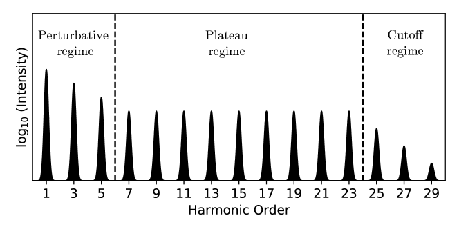
Figure 1.1: A typical high-order harmonic spectrum.

1.2.1 Semiclassical Three-Step Model

An illustration of Corkum’s semiclassical three-step model is presented in Fig. 1.2. The following events can occur in the given order for a bound electron in the presence of a strong oscillating laser field.

1. An intense laser field distorts the Coulombic potential so that the bound electron can tunnel out from the lowered potential barrier.

2. The tunneled electron, initially created with zero kinetic energy, gets accelerated by the influence of the external laser field.

3. When the direction of the laser field reverses, the ionised electron can return and recollide with the parent ion. This recollision can lead to recombination with parent ion, and releases a photon of energy equal to the total energy of the electron.

Here, the second step can be described using the classical equation of motion. Whereas, the first and the third steps require quantum mechanical treatment. In the three-step model, a single-active electron is assumed, and the interaction between electrons is ignored. Let us review strong-field interaction in detail.

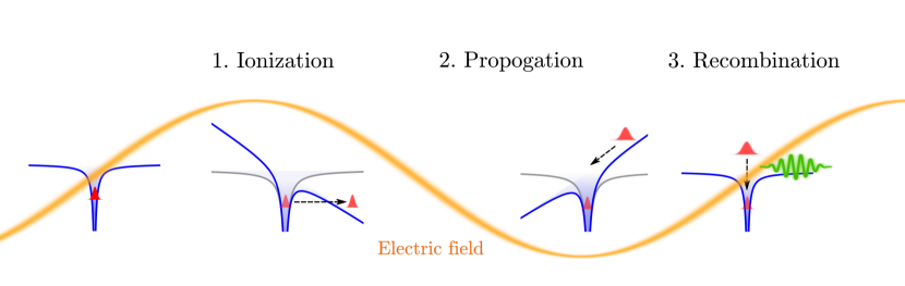
Figure 1.2: Schematic diagram of the three-step model for high-order harmonic generation in atoms.

A typical feature of strong-field interaction mainly originates from the field’s capability of ionisation. There are two ways in which a bound electron can be ionised, either by tunnel ionisation or a transition to continuum via absorption of one or more photons (single or multi-photon ionisation). The mechanism of ionisation is determined by the properties of both the laser and the matter. A general approach to identify the dominant mechanism is based on the dimensionless parameter introduced by Keldysh: Keldysh parameter $\gamma_{{}_{K}}=\sqrt{I_{p}/2U_{p}}$, where $I_{p}$ is the ionisation potential, and $U_{p}$ is the cycle-averaged kinetic energy of a free electron in the presence of a laser field, termed as pondermotive energy. For a laser with central frequency $\omega$, and electric field amplitude $\mathcal{F}_{0}$, the total time-dependent electric field is defined as $\mathcal{F}(t)=\mathcal{F}_{0}\cos(\omega t)$. A free electron in this field experience a force which can be equated to $m\ddot{x}(t)=-e\mathcal{F}_{0}\cos(\omega t)$. The average kinetic energy (pondermotive energy) of a free electron can be calculated from this equation of motion and is equal to

$$U_{p}=\frac{1}{2}m\left\langle\dot{x}(t)^{2}\right\rangle=\frac{e^{2}\mathcal{F}_{0}^{2}}{4m\omega^{2}}.$$ (1.2.1)

$\gamma_{{}_{K}}$ is also defined as the ratio between the tunnelling time of an electron and the laser period. Here, tunnelling time is defined as the time taken by the electron to cross the barrier classically. When the time period of laser is longer, an electron sees a quasi-static potential barrier through which the electron can tunnel ionise. In terms of $\gamma_{K}$, it is when $\gamma_{{}_{K}}\ll 1$, which is valid for intense, long-wavelength laser pulses. On the other hand, multi-photon ionisation is the dominant mechanism when $\gamma_{{}_{K}}\gg 1$. For getting an idea about the value of the Keldysh parameter, let us consider a laser of intensity 10¹⁴ W/cm² and wavelength 800 nm interacting with hydrogen atom, the corresponding value of $\gamma_{{}_{K}}$ is approximately unity (Grossmann, 2018).

Once the electron is freed from the Coulombic potential, it is dominantly influenced by the strong electric-field of the laser. In this interaction regime, understanding the motion of a free electron in the presence of the laser field is important. At intensities higher than 10¹⁸ W/cm², a free electron can acquire velocity comparable with the speed of light. For describing such physics, we need to resort to the relativistic regime of nonlinear optics. Laser sources that can generate pulses as intense as 10²⁰ W/cm² have been developed till now. Typically HHG is observed for laser intensity within the range of 10¹³-10¹⁶ W/cm². Therefore, it is safer to use classical equations of motion for an electron in the laser field. Note that the quantum diffusion of electron wavepacket while propagating in the continuum is neglected here.

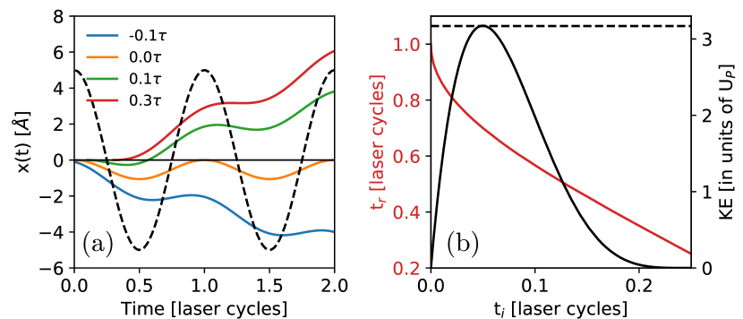
Figure 1.3: (a) Electron trajectories for an electron born at different times during the laser field. Here, $\tau$ is the period of the laser field and $t_{i}$ is the time of ionisation. The dashed line shows the electric field. (b) Kinetic energy of the electron at the time of recombination $t_{r}$ (black line) as a function of time of ionisation $t_{i}$. The dashed vertical line is the maximum energy equal to 3.17$U_{p}$. The time of recombination as a function of time of ionisation (red line).

Consider an electron bound to the nucleus at $x$ = 0. Assuming the electron is tunnel ionised at time $t_{i}$ with zero initial velocity [$\dot{x}(t_{i})$ = 0], the position of electron at any time can be obtained by solving the equation of motion as

$$x(t)=\frac{e\mathcal{F}_{0}}{m\omega^{2}}\left[\cos(\omega t)-\cos(\omega t_{i})+\omega\sin(\omega t_{i})(t-t_{i})\right].$$ (1.2.2)

Electron trajectories obtained from Eq. (1.2.2), for different values of ionisation times $t_{i}$ are shown in Fig. 1.3(a). It is interesting to see that electron born at the peak of laser field returns periodically after each laser cycle. Whereas an electron born before the peak never returns to the ion core. For an electron born after the peak of the laser field, one born earlier, recollide at a later time. This is also evident from the relation of ionisation time and recombination time presented in Fig. 1.3(b) (see red line). The total energy of the electron at the time of recombination, or the high-harmonic photon energy, is given by $\hbar\omega=I_{p}+\textbf{KE}$, where KE is the kinetic energy of an electron at the time of recombination as a function of $t_{i}$, and plotted in Fig. 1.3. Photon of the same energy can be generated from two different trajectories, one short and one long, as apparent from Fig. 1.3. The interference of these trajectories is an important consideration in high-harmonic spectroscopy. The maximum energy of a photon emitted during HHG is given by the relation $\hbar\omega_{c}=I_{p}$ + 3.17$U_{p}$. This implies that the cutoff energy is linearly proportional to the intensity of the laser field. The energy cutoff rule, obtained by the semiclassical model, satisfactorily explains the experimental observations. The underlying mechanism implies that the generation of high-order harmonics is a sub-cycle process, which is the main reason for the generation of attosecond pulses from HHG. Another implication of the semiclassical model of HHG is that the electron ionised using a circularly polarised laser never recombines to the parent ion. Therefore, circularly polarised harmonics can not be generated using a circularly polarised driving pulse efficiently. The harmonic yield decreases drastically when a small value of ellipticity in the driving pulse is introduced.

In general, a physical observable has to be defined to simulate HHG spectrum. In HHG, the Fourier transform of the dipole acceleration serves the purpose. Following Lamor’s theorem of electromagnetism, accelerating charges or time-varying polarisation can act as a source of electromagnetic radiation. Time-dependent dipole can be, respectively, calculated in length, velocity, and acceleration forms as

$$\begin{split}a(t)&=\frac{d^{2}}{dt^{2}}\left\langle\Psi(t)|\hat{x}|\Psi(t)\right\rangle,\\ &=\frac{d}{dt}\left\langle\Psi(t)\right|\hat{p}\left|\Psi(t)\right\rangle,\leavevmode\nobreak\ \leavevmode\nobreak\ \textrm{and}\\ &=\left\langle\Psi(t)\right|-\partial_{x}V\left|\Psi(t)\right\rangle.\end{split}$$ (1.2.3)

Here, $\left|\Psi(t)\right\rangle$ is the time-dependent wavefunction, obtained after solving the time-dependent Schrödinger equation.

Now, let us discuss an important question: why there are only odd harmonics present when high-order harmonics are generated from centerosymmetric systems such as noble-gas atoms. This can be understood from a simple symmetry consideration. When matter interacts with a periodic laser field, the total Hamiltonian can be written as

$$\hat{\mathcal{H}}(t)=\frac{\hat{p}^{2}}{2m}+V(x)+ex\mathcal{F}_{0}\cos(\omega t).$$ (1.2.4)

Here, Hamiltonian is periodic in time as $\hat{\mathcal{H}}(t+\tau)=\hat{\mathcal{H}}(t)$ for $\tau=2\pi/\omega$. Following Floquet theorem of periodically driven quantum systems, a time-periodic Hamiltonian has a wavefunction of the following form as

$$\Psi_{n}(x,t)=e^{-iE_{n}t}\psi_{n}(x,t).$$ (1.2.5)

Here, $\psi_{n}(x,t)$ is the Floquet function which is periodic in time [$\psi_{n}(x,t+\tau)=\psi_{n}(x,t)$]. In the case of a symmetric potential [$V(-x)=V(x)$], Hamiltonian given in Eq. (1.2.4) is invariant under generalised parity transformation $\hat{P}$, $x\rightarrow-x$ and $t\rightarrow t+T/2$. Therefore, Floquet states transform by $\hat{P}$ as $\hat{P}\psi_{n}(x,t)=\pm\psi_{n}(x,t)$.

The contribution to the $n\rm^{th}$-harmonic from the time-dependent dipole moment $d(t)=\left\langle\psi_{n}(t)|\hat{x}|\psi_{n}(t)\right\rangle$, using Fourier transform, is written as (Grossmann, 2018)

$$\begin{split}d_{m}&=\frac{1}{\tau}\int_{0}^{\tau}d(t^{\prime})e^{im\omega t^{\prime}}dt^{\prime}\\ &=\frac{1}{\tau}\left[\int_{0}^{\tau/2}\left\{d(t^{\prime})\pm d(t^{\prime}+\tau/2)\right\}e^{im\omega t^{\prime}}dt^{\prime}\right].\end{split}$$ (1.2.6)

Here, + (-) is for even (odd) value of $m$. It is straightforward to show that

$$\begin{split}d(t+\tau/2)&=\int dx\leavevmode\nobreak\ \psi_{n}^{*}(-x,t)\leavevmode\nobreak\ x\leavevmode\nobreak\ \psi_{n}(-x,t)\\ &=-\int dx\leavevmode\nobreak\ \psi_{n}^{*}(x^{\prime},t)\leavevmode\nobreak\ x^{\prime}\leavevmode\nobreak\ \psi_{n}(x^{\prime},t)\\ &=-d(t).\end{split}$$ (1.2.7)

On substituting the value of Eq. (1.2.7) to Eq. (1.2.6), we can show that there will be only odd harmonics in the spectrum for a material with inversion symmetry.

1.3 High-Harmonic Generation in Solids

Recent advancements in mid-infrared and terahertz laser sources have enabled the generation of strong-field driven HHG from solids, including semiconductors, dielectrics, and nano-structures, below their damage threshold (Ghimire and Reis, 2019; Ghimire et al., 2011a, b; Zaks et al., 2012; Schubert et al., 2014; Vampa et al., 2015b, a; Hohenleutner et al., 2015; Luu et al., 2015; Ndabashimiye et al., 2016; You et al., 2017b; Lanin et al., 2017; Sivis et al., 2017; Langer et al., 2018). With the pioneering work of Ghimire et al. (Ghimire et al., 2011a), HHG in solids offers fascinating avenues to control, understand, and probe light-driven carrier dynamics in solids on attosecond timescale (Silva et al., 2018a, b; Bauer and Hansen, 2018; Chacón et al., 2020; Reimann et al., 2018; Floss et al., 2018; Mrudul et al., 2020).

The difference in the underlying mechanism of HHG from atoms in the gas phase and from solids is presented in Fig. 1.4. Due to the considerable overlap between electron wavefunctions at nearby lattice sites, electron states are best described in the momentum-space using the Bloch theorem. A real-space picture of HHG in solids is shown in Fig. 1.4(a). An electron ionised from a lattice site can propagate over a distance of many lattice periods in real-space. Therefore, it can recombine with any other lattice site other than its parent ion. Yet, due to the lattice periodicity, HHG in solids is a coherent process. As the electron need not recombine with the parent lattice site, the ellipticity dependence of HHG in solids is entirely different. It is possible to generate circularly polarised harmonics using a circularly polarised driving pulse as reported in the pioneering work by Ghimire et al. (Ghimire et al., 2011a). Another contrasting observation in solid HHG is that the energy cutoff depends linearly on the amplitude of the laser’s electric field, whereas a quadratic dependence was reported in HHG from gases. This implies that a reciprocal-space explanation of the underlying mechanism is required.

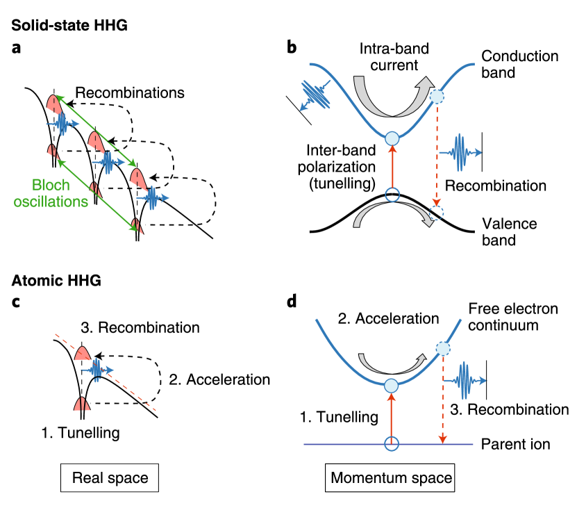
Figure 1.4: A comparative illustration of HHG from atoms and solids. This figure is adapted from Ref. (Ghimire and Reis, 2019).

A reciprocal-space picture of the solid HHG is presented in Fig. 1.4(b). A two-band model for a semiconductor is considered with one valence and one conduction band. The HHG spectrum of solid has two significant contributions: First one is stemming from the time-varying interband polarisation. An electron can be excited to the conduction band by an intense laser-field, and a hole is generated in the valence band. The laser’s electric field can accelerate the electrons and holes in their respective energy bands. This gives the second contribution: an intraband current. In the strong-field regime, interband and intraband contributions are coupled. The role of their contributions in different parts of the spectrum is an interesting area to explore. For example, in the below band-gap region in the spectrum, only intraband current is expected to contribute. Note that, there is no intraband current in atomic HHG as a hole in an atom is expected to be localised [see Fig. 1.4(d)]. When an electron moves adiabatically along a particular conduction band in the absence of scattering, it diffracts from the Brillouin-zone boundaries with a frequency $\omega_{B}=e\mathcal{F}_{0}/\hbar a_{0}$ with $a_{0}$ as the lattice parameter. These diffractions from the zone boundaries give dynamical Bloch oscillations, which result in linear dependence of energy cut off on the laser’s electric-field amplitude in the case of HHG from solids (Ghimire et al., 2011a).

Unlike in gas phase, atoms within a solid possess periodicity and high-electron density. Moreover, high-order harmonics in solids are generated from lasers of intensities in TW/cm² orders, lower compared to the requirements of gas-phase HHG. With all these unique characteristics, HHG from solids offers a compact and superior source for coherent and bright attosecond pulses in extreme ultraviolet and soft x-ray energy regime (Ghimire and Reis, 2019; Luu et al., 2015; Vampa and Brabec, 2017; Kruchinin et al., 2018).

Another exciting aspect of solid HHG is that the harmonic spectrum imprints the anisotropic nature of the lattice. Unlike the two-band model used in Fig. 1.4(b), actual materials include a large number of energy bands, and the high-harmonic spectrum arising from multiple energy bands contains rich information (Hohenleutner et al., 2015; Hawkins et al., 2015). For example, multiple plateau structure in HHG spectrum is observed due to the interband coupling among different pairs of energy bands (Ndabashimiye et al., 2016; Wu et al., 2015). Interestingly, solid HHG is an ideal tool for studying the static and dynamical properties of valence electrons in solids. In recent years, HHG in solids has been employed to explore several exciting processes such as band structure tomography (Vampa et al., 2015b; Lanin et al., 2017; Tancogne-Dejean et al., 2017b), quantum phase transitions (Silva et al., 2018a; Bauer and Hansen, 2018; Silva et al., 2019), the realisation of petahertz current in solids (Luu et al., 2015; Garg et al., 2016), and dynamical Bloch oscillations (Schubert et al., 2014; McDonald et al., 2015).

1.4 Motivation

In this thesis, we thoroughly analyse HHG from hexagonal two-dimensional (2D) materials. Nowadays, 2D materials are at the centre of tremendous research activities as they reveal different electronic and optical properties as compare to their bulk counterparts. The realisation of atomically thin monolayer graphene has led to breakthroughs in fundamental and applied sciences (Novoselov et al., 2004; Geim, 2009). Charge carriers in graphene are described by the massless Dirac equation and exhibit exceptional transport properties (Neto et al., 2009), making graphene very attractive for novel electronics applications. Soon after discovery of graphene, several other 2D materials have been synthesised including hexagonal boron nitride, transition metal dichalcogenides, silicene, germanene, etc. Peculiar electron-photon interaction and electron-localisation makes 2D materials exciting candidates for studying ultrafast electron dynamics.

Monolayer 2D materials such as graphene (Yoshikawa et al., 2017; Al-Naib et al., 2014), transition-metal dichalcogenides (Liu et al., 2017a; Langer et al., 2018), and hexagonal boron nitride (h-BN) (Tancogne-Dejean and Rubio, 2018; Le Breton et al., 2018; Yu et al., 2018) among others have been used to generate strong-field driven high-order harmonics. HHG in h-BN is well studied when the polarisation of the laser pulse is in-plane (Le Breton et al., 2018; Yu et al., 2018) as well as out-of-plane (Tancogne-Dejean and Rubio, 2018) of the material. Using out-of-plane driving laser pulse, Tancogne-Dejean et al. have shown that atomic-like harmonics can be generated from h-BN (Tancogne-Dejean and Rubio, 2018). Also, h-BN is used to explore the competition between atomic-like and bulk-like characteristics of HHG (Tancogne-Dejean and Rubio, 2018; Le Breton et al., 2018). In MoS₂, it has been experimentally demonstrated that the generation of high-order harmonics is more efficient in monolayer in comparison to its bulk counterpart (Liu et al., 2017a). Moreover, HHG from graphene exhibits unusual dependence on the laser ellipticity (Yoshikawa et al., 2017). Langer et al. have demonstrated the control in a light-driven change of the valley pseudospin in WSe₂ (Langer et al., 2018). These works have shed light on the fact that 2D materials are very promising for studying light-driven electron dynamics and for more technological applications in petahertz electronics (Garg et al., 2016) and valleytronics (Schaibley et al., 2016). Furthermore, using atomically thin material helps to avoid macroscopic propagation effects and reabsorption of harmonics by the medium. In this thesis, we aim to investigate few important questions of HHG in 2D materials such as how the attosecond electron dynamics is different in a semimetal and a semiconductor, in a pristine and a defected material, etc.

1.5 Thesis Overview

This thesis consists of six main chapters and a bibliography. At the beginning of each chapter, a brief survey of the literature is presented.

Chapter 1 provides an overview of ultrafast spectroscopy in perturbative and non-perturbative regimes. Furthermore, HHG in gases and solids and their underlying mechanisms are presented. The classic three-step model is discussed in detail. A brief overview of HHG in materials, especially in 2D, materials is presented.

A detailed theoretical framework for understanding HHG in solids is given in Chapter 2. Methods to simulate HHG from model potentials in Cartesian basis and Bloch basis are discussed. This discussion provides reciprocal-space and real-space recollision models for HHG in solids. Moreover, to simulate HHG in real materials, semiconductor Bloch equations and time-dependent density functional theory are introduced.

We discuss HHG from both monolayer and bilayer graphene with the effect of interlayer coupling in bilayer graphene in Chapter 3. Moreover, a comparison of HHG in gapped and gapless graphene and the role of Berry curvature in HHG from gapped graphene are investigated. The effects of polarisation-direction and the ellipticity of the laser pulse on HHG are also presented.

In Chapter 4, we show how tailored laser pulses can generate valley polarisation in a zero band-gap material such as pristine graphene with zero Berry curvature. Also, a recipe to read out the induced valley polarisation is presented.

Chapter 5 discusses the possibility of high-harmonic spectroscopy of spin-polarised defects in hexagonal boron-nitride. The role of boron and nitrogen vacancies in HHG from defected hexagonal boron-nitride is presented. Furthermore, the role of electron-electron interaction is also investigated.

Chapter 6 provides the conclusion and the future scope of the present thesis.

Chapter 2 Theoretical Framework for HHG from Solids

In this chapter, atomic units are used throughout unless stated otherwise. The general recipe for a theoretical understanding of any non-relativistic quantum mechanical phenomena is to solve time-dependent Schrödinger equation (TDSE) as

$${}i\frac{d}{dt}\Psi(\left\{\textbf{r}_{\mu}\sigma_{\mu}\right\},\left\{\textbf{R}_{\nu}\right\},t)=\hat{\mathcal{H}}(t)\Psi(\left\{\textbf{r}_{\mu}\sigma_{\mu}\right\},\left\{\textbf{R}_{\nu}\right\},t).$$ (2.0.1)

Here, $\textbf{r}_{\mu}\sigma_{\mu}$ is the notation for space and spin degrees of freedom of the $\mu^{\textrm{th}}$ electron, and $\textbf{R}_{\nu}$ stands for the positions of the $\nu^{\textrm{th}}$ ion-core. In Eq. (2.0.1), nuclei’s kinetic-energy can be neglected since these are much heavier than electrons. Consequently, the electron and nucleus degree of freedom can be separated. Throughout this work, we considered frozen nuclei and any effects arising from lattice vibrations are neglected. Therefore, our objective is to solve TDSE for electrons in the presence of light as

$${}i\frac{d}{dt}\Psi_{e}(\left\{\textbf{r}_{\mu}\sigma_{\mu}\right\},t)=[\hat{\mathcal{H}_{0}}+\hat{\mathcal{H}}^{\prime}(t)]\Psi_{e}(\left\{\textbf{r}_{\mu}\sigma_{\mu}\right\},t).$$ (2.0.2)

Here, $\hat{\mathcal{H}_{0}}$ is the field-free Hamiltonian and $\mathcal{\hat{H}}^{\prime}(t)$ is the light-matter interaction Hamiltonian. The field free Hamiltonian is given by $\hat{\mathcal{H}_{0}}=\hat{T}_{e}+\hat{V}_{e-i}+\hat{W}_{e-e}$. Here, $\hat{T}_{e}=\sum_{\mu=1}^{N}-\nabla_{\mu}^{2}/2$ is the kinetic energy operator, $\hat{V}_{e-i}=\sum_{\mu=1}^{N}v(\textbf{r}_{\mu})$ is the Coulomb attraction between electron and ion-core, and $\hat{W}_{e-e}=\frac{1}{2}\sum_{\mu\neq\nu}^{N}w(|\textbf{r}_{\mu}-\textbf{r}_{\nu}|)$ is the electron-electron Coulomb interaction. It is essential to point out that the ion-core coordinates enter in the electronic Hamiltonian as parameters in $\hat{V}_{e-i}$. Therefore, $\hat{V}_{e-i}$ is the term that distinguishes different electronic systems. The time-dependent interaction Hamiltonian is given by $\mathcal{\hat{H}}^{\prime}(t)=-\sum_{\mu}\textbf{r}_{\mu}\cdot\mathcal{F}(t)$, where $\mathcal{F}(t)$ is the electric field. Owing to the large wavelength of the field compared to the lattice parameters, dipole approximation is employed in this thesis. Therefore, the spatial dependence of the field is neglected.

The $W_{e-e}$ term essentially makes Eq. (2.0.2) a $6N\times 6N$ coupled differential equation, which is not exactly solvable except for few systems such as hydrogen. Moreover, in the strong-field limit, the magnitude of the interaction Hamiltonian $\hat{\mathcal{H}}^{\prime}(t)$ is comparable to $\hat{\mathcal{H}_{0}}$, which prevents us from using perturbative treatments. The way to solve such a problem is by numerically propagating TDSE with reliable approximations.

This chapter is designed as follows: In Section 2.1, we discuss about solving TDSE for a model periodic potential. In Section 2.2, we will analyse HHG spectrum for a model periodic potential and discuss the basic mechanism. In Section 2.3, we discuss how the theoretical methods can be extended to realistic solids.

2.1 HHG from a Model Potential

In this section, we neglect electron-electron interaction potential [W_e-e in Eq. (2.0.2)]. To model the periodic electron-nuclear (V_e-i) interaction in solids, we use an one-dimensional periodic potential and corresponding TDSE is written as

$$i\frac{d}{dt}\left|\psi(t)\right\rangle=\left[\hat{\mathcal{H}}_{0}+\hat{\mathcal{H}}^{\prime}(t)\right]\left|\psi(t)\right\rangle.$$ (2.1.1)

Here, $\hat{\mathcal{H}}_{0}=-\nabla^{2}/2+V(\hat{x})$ with $V(x)$ as a periodic potential. The laser polarization is considered along the crystal axis.

The Mathieu-type model potential is expressed as

$$V(x)=-V_{0}[1+\cos(2\pi x/a)].$$ (2.1.2)

Here, $a$ is the lattice parameter, and $-2V_{0}$ is the depth of the potential as shown in Fig. 2.1(a). This is a commonly used potential for modelling HHG from solids (Wu et al., 2015; Liu et al., 2017c; Ikemachi et al., 2017).

In the following subsections, we show two different approaches to solve TDSE for model periodic potential. We use a lattice parameter, $a$ = 8 a.u. and $V_{0}$ = 0.37 a.u. for the study, similar to Refs. (Wu et al., 2015; Liu et al., 2017c, b; Ikemachi et al., 2017).

2.1.1 Cartesian Basis

In this approach, the numerical methods developed for atoms are extended for a periodic potential. The method is adapted from Ref. (Liu et al., 2017b). $\hat{\mathcal{H}}_{0}$ is diagonalised in cartesian space to obtain the eigen-spectrum of the periodic lattice as

$$\hat{\mathcal{H}}_{0}\psi_{n}(x)=\mathcal{E}_{n}\psi_{n}(x).$$ (2.1.3)

The coordinate space within the region [-800 a.u., 800 a.u.] is considered, which corresponds to 200 lattice periods. The grid-spacing of 0.25 a.u. is used. For a wide-band-gap semiconductor, all valence-band electronic-states are filled, and all conduction-band electronic-states are empty. Owing to the low excitation probability considered in the present work, we choose the highest occupied (ho) eigenstate as the ground-state wave function [$\phi(x,t=0)=\psi_{ho}(x)$]. The light-matter interaction is modelled in length gauge as $\hat{\mathcal{H}}^{\prime}(t)=\hat{x}\mathcal{F}(t)$. Time-dependent wave function $\phi(x,t)$ is obtained by solving TDSE numerically using split-operator method (Hermann and Fleck Jr, 1988) with a time-step 0.03 a.u. At each time-step, the wave function is multiplied with a mask function of width 100 a.u. to avoid unphysical reflection from the boundaries.

The expectation value of the derivative of current, $j(t)$ at any particular time, using acceleration form is proportional to

$$\frac{d}{dt}j(t)\propto\int\frac{\partial V}{\partial x}\leavevmode\nobreak\ |\psi(x,t)|^{2}\leavevmode\nobreak\ dx.$$ (2.1.4)

The high-harmonic spectrum can be calculated as

$$\mathcal{I}(\omega)=\left|\mathcal{FT}\left[\frac{d}{dt}j(t)\right]\right|^{2}.$$ (2.1.5)

Here, $\mathcal{FT}$ stands for Fourier transform. To obtain high-harmonic spectrum, a linearly polarised laser pulse of wavelength 3.2 $\mu$m and intensity 0.8 TW/cm² is used in the simulation. The pulse contains eight optical cycles with sine-square envelope. The values of wavelength and intensity mimic the values used in the experiment performed by Ghimire et al. (Ghimire et al., 2011a). To avoid material damage, long wavelength and lower intensity in comparison to HHG from gases are used. The corresponding HHG spectrum obtained is presented in Fig. 2.1(b) (violet).

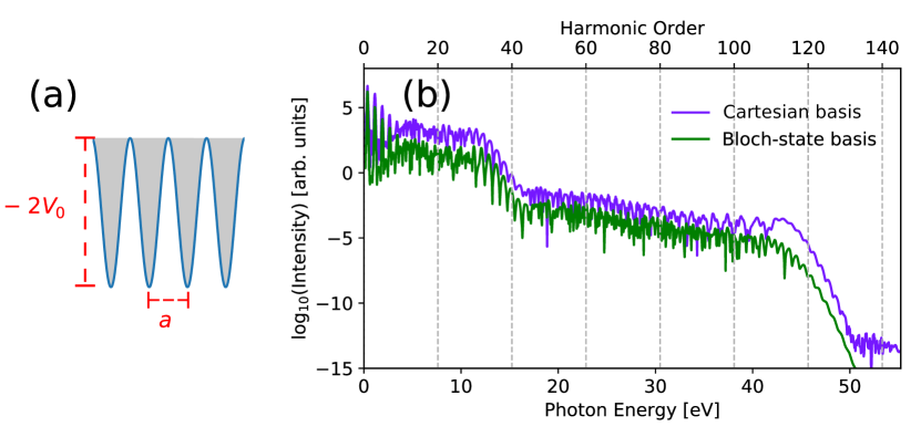
Figure 2.1: (a) Mathieu-type potential. (b) High-harmonic spectrum simulated for the Mathieu-type potential simulated in Cartesian (violet) and Bloch-state basis (green). Here, the laser has an intensity of 0.8 TW/cm² and a wavelength of 3.2 $\mu$m.

2.1.2 Bloch-State Basis

In this subsection, we make use of the periodicity of the lattice by using Bloch functions as basis. To preserve the lattice-periodicity in the total Hamiltonian, we consider $\hat{\mathcal{H}}^{\prime}(t)$ in velocity gauge as $\hat{\mathcal{H}}^{\prime}(t)=\hat{p}\cdot\mathcal{A}(t)$. Here, $\mathcal{A}(t)$ is the vector potential of the driving laser-field and it is related to electric field $\mathcal{F}(t)$ as $\mathcal{F}=-\partial\mathcal{A}/\partial t$. The eigenstates of $\hat{\mathcal{H}}_{0}$ is obtained in Bloch-state basis as

$$\hat{\mathcal{H}}_{0}\left|\phi_{nk}\right\rangle=\mathcal{E}_{nk}\left|\phi_{nk}\right\rangle.$$ (2.1.6)

Here, $n$ is the band index and $k$ is the wavevector. Solution to Eq. (2.1.6) is Bloch functions defined as $\phi_{nk}(x)=e^{ikx}u_{nk}(x)$ and $u_{nk}(x)$ has the periodicity of the lattice.

The Bloch functions at different k-points can be propagated independently within dipole approximation. For a particular k-point, the time-dependent wave function can be expanded in Bloch-state basis as (Wu et al., 2015),

$$\left|\psi_{k}(t)\right\rangle=\sum_{n}\alpha_{nk}(t)\left|\phi_{nk}\right\rangle.$$ (2.1.7)

Substituting Eq. (2.1.7) in TDSE [Eq. (2.1.1)] within velocity-gauge and multiplying with $\left\langle\phi_{mk}\right|$ yields

$$i\frac{\partial}{\partial t}\alpha_{nk}=\alpha_{nk}\mathcal{E}_{nk}+\mathcal{A}(t)\sum_{m}p^{nm}_{k}\alpha_{mk}.$$ (2.1.8)

Here, $p_{nm}^{k}$ is the momentum-matrix elements defined as $p_{nm}^{k}=\left\langle\phi_{nk}\right|\hat{p}\left|\phi_{mk}\right\rangle$. We solve Eq. (2.1.8) using a fourth-order Runge-Kutta method with a time-step of 0.01 a.u (Korbman et al., 2013). The high-harmonic spectrum is calculated as

$$\mathcal{I}(\omega)=\left|\mathcal{FT}\left[\frac{d}{dt}\int j(k,t)\leavevmode\nobreak\ dk\right]\right|^{2}.$$ (2.1.9)

Initially all the valence bands are expected to be filled. However, since we are only considering low excitation probability, we have assumed only 3$\%$ occupation near the highest occupied valence band. Other deeply bound valence bands are neglected in the calculation. The spectra were converged for the number of conduction bands. Similar approximations are used in Ref. (Wu et al., 2015).

Finally, we calculated the HHG spectrum for the potential and laser parameters used in subsection 2.1.1 and presented in Fig. 2.1(b)(green). The HHG spectrum calculated by both the methods agree quite well and have important features. In the next section, we discuss how the mechanism of HHG can be understood from this simple model.

2.2 Mechanism of HHG in Solids

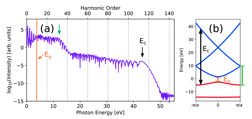
Figure 2.2: (a) The simulated high-harmonic spectrum for the Mathieu-type potential, for the same laser parameters used in  2.1(b). The vertical orange line indicates the minimum band-gap (E_g). (b) The electronic band-structure corresponds to the Mathieu-type potential. Valence and conduction bands are shown in red and blue colours, respectively.

In this section, we do a detailed investigation of the underlying mechanism of HHG in solids. Unlike a simple three-step recollision model in gases, the mechanism of HHG is quite different in solids. In subsection 2.2.1, we show how the HHG spectrum can be understood from the electronic band-structure. In subsection 2.2.2, we show how a real-space recollision model can be developed to understand HHG in solids.

2.2.1 A Reciprocal-Space Understanding

The simulated spectrum of solid HHG reproduces exciting features as presented in Fig. 2.2(a). The major features can be listed as follows a) there are clear harmonic peaks with monotonically decreasing intensity up to particular energy, b) it exhibits both a primary and a secondary plateaus and a sudden transition from primary to secondary plateaus with clear cutoffs, and c) the harmonic signal in the plateau region is noisy.

Let us try to understand the mechanism of HHG from the corresponding band-structure of the Mathieu potential presented in Fig. 2.2(b). The valence bands are shown in red color, whereas conduction bands are shown in blue colour. The electron can have two types of dynamics in solids: the intraband dynamics originating from an electron (hole) accelerating in a conduction (valence) band, and the contribution from the interband transitions as a result of the recombination of an electron from conduction band to a hole in a valence band.

In the energy-band structure, the minimum band-gap (E_g) is at 4.19 eV [marked in orange color in Figs. 2.2(a) and 2.2(b)]. In the below band-gap region, interband transitions are not possible, and those transitions are purely intraband. In the above band-gap region, there can be contributions from interband and intraband transitions, which interfere and gives the noisy signal. Assuming infinite dephasing time is also found out to be a reason for the noisy spectra (Vampa et al., 2014). The primary plateau lies between E_g and 12.86 eV. Here, the primary energy cutoff corresponds to the maximum energy between the first conduction and valence bands. Moreover, the secondary energy cutoff (E_c) is at 44.23 eV, which is less than the maximum band-gap energy between third conduction and valence bands.

These results are in good agreement with the previously published results (Wu et al., 2015; Liu et al., 2017a; Ikemachi et al., 2017). The primary plateau arises due to the interband transition from the first conduction band to the valence band. The electron can also move to the higher conduction band via interband tunnelling [see e.g. (Hawkins et al., 2015; Ndabashimiye et al., 2016; Ikemachi et al., 2017)]. Transitions from the higher-lying conduction band to the valence band lead to the secondary plateau, e.g. (Ndabashimiye et al., 2016). Since the interband transitions between the second conduction and valence band is less probable compared to the transitions between the first conduction and valence band, the secondary plateau is about five orders of magnitude lower than the primary plateau.

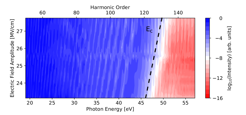
Figure 2.3: High-harmonic spectrum as a function of electric field strength. The energy region of the secondary plateau is shown and the black dashed line indicates the energy cutoff (E_c).

We have established how the band-structure information is embedded in the harmonic spectrum using an interband explanation. Now we analyse how the intraband mechanism plays a role in the electric field dependence of energy cutoff. High-harmonic spectrum as a function of electric field amplitude is presented in Fig. 2.3. The energy cutoff (E_c) in the second plateau varies linearly with the field amplitude of driving laser as is typical for solids (Ghimire et al., 2011a, 2014; Wu et al., 2015; Du and Bian, 2017). This is in-contrast to the case of atomic-HHG, where the cutoff scales quadratically with the electric field amplitude as a consequence of the three-step-model. The reason for the linear dependence is explainable using dynamical Bloch oscillations, where the Bloch frequency is directly proportional to the electric-field amplitude (Ghimire et al., 2011a).

2.2.2 A Real-Space Recollision Model

Here we describe results of our numerical experiment, which allows us to link directly HHG in solids with real-space electron-hole recollision. We take advantage of the angstrom-scale spatial resolution embedded in the harmonic signal, well established in molecules (Smirnova et al., 2009; Haessler et al., 2010; Lein et al., 2002b, a; Lein, 2007; Vozzi et al., 2005; Kanai et al., 2005; Odžak and Milošević, 2009; Torres et al., 2010; Sukiasyan et al., 2010). The spatial information arises from half-scattering during electron-molecule recombination. It manifests in characteristic minima in the HHG spectra (Lein et al., 2002b, a; Lein, 2007). The characteristic minima are laser-intensity independent (Smirnova et al., 2009; Lein et al., 2002b, a; Lein, 2007) and are associated with structure-based minima in the photorecombination cross sections (Lein et al., 2002b, a; Lein, 2007; Vozzi et al., 2005; Kanai et al., 2005; Odžak and Milošević, 2009; Torres et al., 2010; Sukiasyan et al., 2010), mirroring the well-known structure-related minima in photoionization. In diatomic molecules, the minima result from the Cohen-Fano interference of the two photoionization pathways originating at the two nuclei (Cohen and Fano, 1966).

Clearly, if real-space recollision between the conduction-band electron and the valence-band hole underlies HHG in solids, it is supposed to exhibit the same Cohen-Fano type interference minima when the unit cell of the periodic lattice potential has a two-centre structure. In our study, we restrict ourselves to wide band-gap materials, low-frequency drivers, and low excitation probability, where effective single-particle description is adequate.

To explore the idea, we model a semiconductor with two atom basis. In such a case, there will be two characteristic lengths for the unit-cell, the inter-atomic distance as well as the lattice constant. When the laser polarization is along the direction of the interatomic bond, we can effectively model this system using a one-dimensional bichromatic lattice potential as shown in Fig. 2.4(a) and can be expressed as

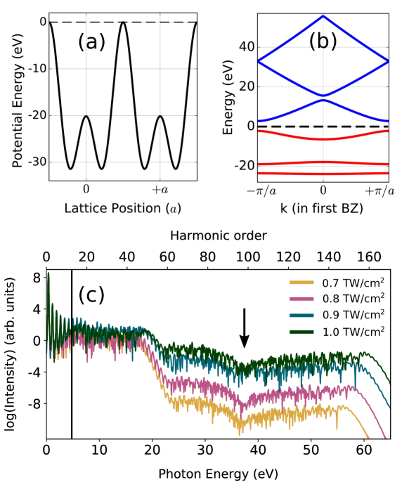
Figure 2.4: A bichromatic potential (a) and the corresponding band-structure with valence (red) and conduction bands (blue) marked. (b) High-harmonic spectrum as a function of driving laser intensity for the bichromatic lattice. The black arrow represents the position of the minimum.

$$V(x)=-V_{0}\left[(\alpha+\beta)-\alpha\cos\left(\frac{4\pi x}{a}\right)-\beta\cos\left(\frac{2\pi x}{a}\right)\right].$$ (2.2.1)

Here, $V_{0}$ is the potential depth, $a$ is the lattice constant. Each unit cell has a double-well shape, with $a$ the distance between the unit cells [see Fig. 2.4(a)], and the ratio of $\alpha$ and $\beta$ control the depth of the double-well potential. In the present study, $V_{0}=0.37$ a.u., $a=8$ a.u. and $\alpha=\beta=1$ are used. Fig. 2.4(b) shows the energy-band structure within the first Brillouin Zone for this bichromatic lattice. The minimum energy band-gap is 4.99 eV at the edge of the Brillouin zone ($k=\pm\pi/a$).

To ensure the robustness of our findings, we have also simulated the HHG spectra by solving TDSE in real-space. The results obtained from two different numerical approaches, in real-space and in the Bloch state basis, show excellent agreement with each other.

For the bichromatic lattice, the HHG spectrum is shown in Fig. 2.4(c), for an eight optical cycles linearly polarised laser pulse with a sine-square envelope and $\lambda=3.2\leavevmode\nobreak\ \mu$m. Spectra corresponding to the four different laser intensities are shown, 0.7 TW/cm² (yellow), 0.8 TW/cm² (pink), 0.9 TW/cm² (blue) and 1.0 TW/cm² (green). The spectra exhibit both a primary and a secondary plateau and a sharp transition from the primary to the secondary plateau, with clear cutoffs.

The multiple-plateau structure and energy cutoff of HHG spectrum [Fig. 2.4(c)] are consistent with the corresponding band-structure [Fig. 2.4(b)] as explained in the subsection 2.2.1. The intensity of the second plateau increases with the laser intensity, see Fig. 2.4, reflecting higher probability of the inter-band excitation to the higher conduction band. The monotonically increasing cutoff with respect to laser intensity is also consistent with the linear cutoff dependence explained in subsection 2.2.1.

The key feature of interest is the pronounced minimum in the second plateau, clearly present in Fig. 2.4(c) (see black arrow). To identify its physical origin, we plot the position of the minimum as a function of the laser intensity in Fig. 2.5(a). It shows that the position of the minimum is not sensitive to the laser intensity, just like the Cohen-Fano type interference minimum in HHG from molecules  (Lein et al., 2002b, a; Lein, 2007; Kanai et al., 2005; Vozzi et al., 2005; Boutu et al., 2008; Zhou et al., 2008; Odžak and Milošević, 2009; Torres et al., 2010).

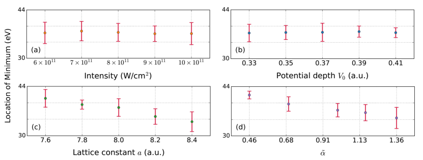
Figure 2.5: The variation in the position of the minimum in high-harmonic spectrum as a function of (a) intensity of the driving laser ($\lambda$ = 3.2 $\mu$m, V₀ = 0.37 a.u., and $a$ = 8 a.u.), (b) potential depth V₀ for the fixed lattice constant ($a$ = 8 a.u.), (c) as a function of the lattice constant ($a$) (for V₀ = 0.37 a.u.), and (d) as a function of the depth of the double-well potential $\tilde{\alpha}=\alpha/\beta^{2}$ (for V₀ = 0.37 a.u., $a$ = 8 a.u.). In (b)-(d), the laser intensity I = 0.8 TW/cm² was used. The error bar represents the width of the interference minimum.

To verify this conclusion, we look at the position of the minimum as a function of the parameters of the bichromatic lattice potential [see Eq. (2.2.1)]. As expected for the Cohen-Fano type interference in radiative recombination during recollision, the position of the minimum is independent of the depth of the bichromatic potential ($V_{0}$) as long as the distance between the wells does not change, see Fig. 2.5(b). However, the position of the minimum changes as soon as we start to vary the lattice constant $a$, see Fig. 2.5(c). As the lattice constant is increased, the minimum shifts towards lower photon energies as it should be. Identical observations have been reported for oriented molecules, where the interference minimum occurs at a lower harmonic order for larger internuclear bond-length, (or when the aligned molecular ensemble is rotated towards the field polarization)  (Lein et al., 2002b, a). As can be seen from Eq. (2.2.1), the ratio of $\alpha$ and $\beta$ controls the depth of the double-well potential. Changing this ratio changes the depth of the potential barrier between the two wells, and thus the distance between the two peaks of the corresponding wave function. For small $\tilde{\alpha}=\alpha/\beta^{2}$, the distance between the two peaks in the double-well wave function is smaller, and so the minimum is shifted to higher energies as evident from Fig. 2.5(d). Note that, the harmonic spectrum from single colour lattice (monochromatic lattice) does not exhibit any minimum in the spectrum. Therefore, analogous to structural minimum in oriented molecules, this minimum in solid HHG is related to the structure of the potential.

In diatomic molecules, the structural minimum associated with photorecombination disappears when the two nuclei are substantially different, so that the ground state is localized on a single nucleus. The same should happen here.

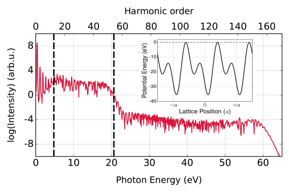
Figure 2.6: High-harmonic spectrum for the asymmetric bichromatic periodic lattice (shown in inset). The harmonic spectrum is obtained for intensity of 0.8 TW/cm² and wavelength of 3.2 $\mu$m. Here, the vertical dashed lines at 4.8 eV and 20.6 eV, respectively, the minimum and maximum band-gaps between the first conduction band and the valence band.

To check this effect, we introduce asymmetry into the double-well potential of the lattice as shown in Fig. 2.6 (inset). The asymmetry is introduced by adding a 90^∘ phase difference between the two spatial frequency components of the lattice. The corresponding harmonic spectrum is shown in Fig. 2.6 for I = 0.8 TW/cm² and $\lambda=3.2\leavevmode\nobreak\ \mu$m. While the overall harmonic spectrum is the same as for the symmetric bichromatic potential [see Figs.  2.4(c) and  2.6], the minimum disappears. Therefore, the minimum in solid HHG does indeed represent the structural minimum in recombination, in direct analogy with HHG in molecules, providing clear evidence of the recollision picture of HHG in solids.

2.3 HHG from Realistic Solids

At this stage, it is important to go beyond the periodic model potential and understand the electron dynamics in realistic systems. This helps one to understand the symmetries, effect of dephasing, appreciate the role of interband and intraband mechanisms as well as the effect of electron-electron interactions in solid HHG. For these purposes, we introduce two approaches in this section as

1. Semiconductor Bloch equations (SBE), where the single electron TDSE can be solved for a few electronic bands of a realistic solid.

2. Time-dependent density functional theory (TDDFT), in which the electron-electron interaction can be also incorporated.

2.3.1 Semiconductor Bloch Equations

The electron dynamics in semiconductors in the presence of strong lasers can be theoretically modelled by SBE (Haug and Koch, 2009). Recently, SBE is extensively used in high-harmonic spectroscopy of solids (Vampa et al., 2014; Hohenleutner et al., 2015; Jiang et al., 2018). SBE allow us to separate interband and intraband contributions in the HHG spectrum (Wu et al., 2015). Moreover, it helps us to understand the effect of dephasing. The adiabatic equation for Bloch electrons in Houston basis is written as

$$\hat{H}(t)\left|\phi^{H}_{n,\textbf{k}_{0}}\right\rangle=\mathcal{E}_{n}(\textbf{k}(t))\left|\phi^{H}_{n,\textbf{k}_{0}}\right\rangle.$$ (2.3.1)

Here, $\left|\phi^{H}_{n,\textbf{k}_{0}}\right\rangle$ is the instantaneous eigenstate for a Bloch electron and $\textbf{k}(t)=\textbf{k}_{0}+\mathcal{A}(t)$. Eq. (2.3.1) is not equivalent to TDSE, but $\left\{\phi^{H}_{n,\textbf{k}_{0}}\right\}$ form a complete basis. The Houston basis functions are related to the Bloch basis function with crystal momentum $\textbf{k}(t)$ as

$$\left|\phi^{H}_{n,\textbf{k}_{0}}(t)\right\rangle=e^{-i\mathcal{A}\cdot\hat{\textbf{r}}}\left|\phi^{B}_{n,\textbf{k}(t)}\right\rangle,$$ (2.3.2)

where $\left\langle\hat{\textbf{r}}\right.\left|\phi^{B}_{n,k(t)}\right\rangle=e^{i\textbf{k}(t)\cdot\textbf{r}}u_{n,\textbf{k}(t)}(\textbf{r})$.

Let $\left|\psi(t)\right\rangle$ be the wave function, which fulfils TDSE as

$$i\frac{d}{dt}\left|\psi(t)\right\rangle=\left[\frac{1}{2}(\hat{\textbf{p}}+\mathcal{A}(t))^{2}+V(\hat{\textbf{r}})\right]\left|\psi(t)\right\rangle.$$ (2.3.3)

Here, $\left|\psi(t)\right\rangle$ can be expanded in Houston basis as

$$\left|\psi(t)\right\rangle=\sum_{n,\textbf{k}_{0}}a_{n,\textbf{k}_{0}}(t)\left|\phi^{H}_{n,\textbf{k}_{0}}(t)\right\rangle.$$ (2.3.4)

Substituting Eq. (2.3.4) in Eq. (2.3.3) and taking an inner product with $\left\langle\phi^{H}_{m,\textbf{k}_{0}}\right|$ gives

$$i\sum_{n,\textbf{k}_{0}}\left[\dot{a}_{n,\textbf{k}_{0}}(t)\delta_{nm}+a_{n,\textbf{k}_{0}}(t)\left\langle\phi^{H}_{m,\textbf{k}_{0}}\right|\partial_{t}\left|\phi^{H}_{n,\textbf{k}_{0}}(t)\right\rangle\right]=\sum_{n,k_{0}}a_{n,\textbf{k}_{0}}\mathcal{E}(\textbf{k}(t))\delta_{nm}.$$ (2.3.5)

The matrix elements, $\left\langle\phi^{H}_{m,\textbf{k}_{0}}(t)\right|\partial_{t}\left|\phi^{H}_{n,\textbf{k}_{0}}(t)\right\rangle$ can be simplified as,

$$\left\langle\phi^{H}_{m,\textbf{k}_{0}}(t)\right|\partial_{t}\left|\phi^{H}_{n,\textbf{k}_{0}}(t)\right\rangle=-\mathcal{F}(t)\cdot\left\langle u_{m,\textbf{k}(t)}\right|\nabla_{\textbf{k}}\left|u_{n,\textbf{k}(t)}\right\rangle.$$ (2.3.6)

On substituting Eq. (2.3.6) in Eq. (2.3.5) and simplifying gives (Wu et al., 2015) us

$$i\partial_{t}a_{m,\textbf{{k}}_{0}}=\epsilon_{m}^{\textbf{k}_{0}+\mathcal{A}(t)}a_{m,\textbf{k}_{0}}-\mathcal{F}(t)\cdot\sum_{n}\textbf{d}_{mn}^{\textbf{k}_{0}+\mathcal{A}(t)}a_{n,\textbf{k}_{0}},$$ (2.3.7)

where $\textbf{d}_{nm}^{\textbf{k}}$ is defined as $i\left\langle u_{n,\textbf{k}}\right|\nabla_{\textbf{k}}\left|u_{m,\textbf{k}}\right\rangle$. A set of equations equivalent to Eq. (2.3.7) in terms of density matrix elements can be derived by defining the density matrix elements, $\rho_{mn}^{\textbf{k}_{0}}=a_{m,\textbf{k}_{0}}a{{}^{*}}_{n,\textbf{k}_{0}}$ and solving Eq. (2.3.7).

$$\frac{\partial}{\partial t}\rho_{mn}^{\textbf{k}_{0}}=-i\mathcal{E}_{mn}^{\textbf{k}_{0}+\mathcal{A}(t)}\rho^{\textbf{k}_{0}}_{mn}+i\mathcal{F}(t)\cdot\left[\sum_{l}\left(\textbf{d}_{ml}^{\textbf{k}_{0}+\mathcal{A}(t)}\rho_{ln}^{\textbf{k}_{0}}-\textbf{d}_{ln}^{\textbf{k}_{0}+\mathcal{A}(t)}\rho_{ml}^{\textbf{k}_{0}}\right)\right],$$ (2.3.8)

where $\mathcal{E}^{\textbf{k}}_{mn}$ is the band-gap energy between $m$ and $n$ bands at k. A phenomenological term accounting for the decoherence can be added, with a constant dephasing time $T_{2}$, the semiconductor Bloch equations are given by

$$\partial_{t}\rho_{mn}^{\textbf{k}_{0}}=\left[-i\mathcal{E}_{mn}^{\textbf{k}_{0}+\mathcal{A}}-\frac{\tilde{\delta}_{mn}}{T_{2}}\right]\rho_{mn}^{\textbf{k}_{0}}+i\mathcal{F}\cdot\left[\sum_{l}\left(\textbf{d}_{ml}^{\leavevmode\nobreak\ \textbf{k}_{0}+\mathcal{A}}\rho_{ln}^{\textbf{k}_{0}}-\textbf{d}_{ln}^{\leavevmode\nobreak\ \textbf{k}_{0}+\mathcal{A}}\rho_{ml}^{\textbf{k}}\right)\right].$$ (2.3.9)

Here, $\tilde{\delta}_{mn}$ is defined as (1-$\delta_{mn}$). The term accounts for the band population relaxation ($T_{1}$) is neglected assuming $T_{1}$ $\gg$ $T_{2}$ (Hwang and Sarma, 2008).

The current at any $\bf{k}$-point in the Brillouin zone can be calculated as

$$\begin{split}\textbf{J}^{\textbf{k}}(t)&=\sum_{m,n}\rho_{mn}^{\textbf{k}}(t)\leavevmode\nobreak\ \textbf{p}_{nm}^{\leavevmode\nobreak\ \textbf{k}+\mathcal{A}}\\ &=\sum_{m\neq n}\rho_{mn}^{\textbf{k}}(t)\leavevmode\nobreak\ \textbf{p}_{nm}^{\leavevmode\nobreak\ \textbf{k}+\mathcal{A}}+\sum_{m=n}\rho_{m,n}^{\textbf{k}}(t)\leavevmode\nobreak\ \textbf{p}_{nm}^{\leavevmode\nobreak\ \textbf{k}+\mathcal{A}}\\ &=\textbf{J}_{inter}^{\textbf{k}}(t)+\textbf{J}_{intra}^{\textbf{k}}(t).\end{split}$$ (2.3.10)

Here, $\textbf{J}_{inter}^{\textbf{k}}(t)$ and $\textbf{J}_{intra}^{\textbf{k}}(t)$ are, respectively, interband and intraband contributions to the total current, and p${}_{nm}^{\textbf{k}}$ is momentum matrix element, which can be obtained as $\textbf{p}_{nm}^{\textbf{k}}=\left\langle n,\textbf{k}\left|\nabla_{\textbf{k}}\hat{\mathcal{H}}_{\textbf{k}}\right|m,\textbf{k}\right\rangle$. The off-diagonal elements of momentum and dipole-matrix elements are related as $\textbf{d}^{\textbf{k}}_{mn}$ = $i\textbf{p}^{\textbf{k}}_{mn}/\mathcal{E}^{\textbf{k}}_{mn}$. Here, with the knowledge of band-structure, dipole and momentum matrix elements, Eq. (2.3.9) can be solved for any realistic material.

We used length gauge due to the following reasons. In a basis involving infinite bands, any physical observable measured from SBE is gauge invariant. In contrast, for a model involving finite number of bands, the nonlinear response of semiconductors depends on the laser-gauge choice. For such a truncated basis, velocity gauge calculations have many disadvantages over length gauge, as the calculation only converges for numerous bands, and there is divergence at small frequencies.

The structure gauge choices don’t affect the velocity gauge calculations, as each k-point is treated independently. On the other hand, for the length gauge calculation, the relative phase of the wave function in the reciprocal-space is critical. The phase of the wave function should be continuous and periodic. This problem can be fixed either by obtaining wavefunctions analytically or by using the twisted parallel transport gauge (Yue and Gaarde, 2020).

The high-harmonic spectrum is determined from the Fourier-transform of the time-derivative of the current as

$$\mathcal{I}(\omega)=\left|\mathcal{FT}\left(\frac{d}{dt}\left[\int_{BZ}\textbf{J}(\textbf{k},t)\leavevmode\nobreak\ \rm d\textbf{k}\right]\right)\right|^{2}.$$ (2.3.11)

Here, integration is performed over the entire Brillouin zone.

2.3.2 Time-Dependent Density Functional Theory

There are situations where electron-electron interaction becomes extremely important as recently demonstrated by TDDFT study of HHG (Tancogne-Dejean and Rubio, 2018; Tancogne-Dejean et al., 2018). In this subsection, we briefly present the theory of TDDFT for HHG in solids.

Density functional theory (DFT) is a popular method to solve electronic structure problem. Our goal is to solve TDSE with electron-electron interaction [Eq. (2.0.2)]. For that, we will start our discussion by reviewing the ground-state DFT, where the time-independent Schrödinger equation corresponding to Eq. (2.0.2) is expressed as

$$\left[\hat{T}_{e}+\hat{V}_{e-i}+\hat{W}_{e-e}\right]\Psi_{0}(\left\{\textbf{r}\sigma\right\})=\mathcal{E}\Psi_{0}(\left\{\textbf{r}\sigma\right\}).$$ (2.3.12)

Here, $\Psi_{0}$ is the ground state wave function. In their seminal work, Hohenberg and Kohn showed that any quantum mechanical property of a many-electron system can be deduced from their ground-state density, $n_{0}(\textbf{r})$, without the requirement of the many-electron wave function $\Psi_{0}$ (Hohenberg and Kohn, 1964). This is the foundation of DFT.

For any non-relativistic quantum mechanical system, the form of $\hat{T}_{e}$ and $\hat{W}_{e-i}$ are universal. On the other hand, $\hat{V}_{e-i}$ characterise the system. Hohenberg and Kohn showed that there is a one-to-one mapping between $v_{ei}(\textbf{r})$ and $n_{0}(\textbf{r})$, whereas $\Psi_{0}$ is a unique functional of $n_{0}(\textbf{r})$. This imply that the ground-state density contains all the information of the electronic system. Consequently, any observable $\hat{O}$ is also a unique functional of $n_{0}(\textbf{r})$ as $O[n_{0}]=\left\langle\Psi_{0}[n_{0}]\right|\hat{O}\left|\Psi_{0}[n_{0}]\right\rangle$. In particular, ground-state energy functional can be defined as

$$E[n_{0}]=\left\langle\Psi_{0}[n_{0}]\right|\mathcal{\hat{H}}_{0}\left|\Psi_{0}[n_{0}]\right\rangle.$$ (2.3.13)

However, the exact energy functional can be found out variationally. Expressing the energy functional in terms of single-particle orbitals $\phi_{\mu}$, we obtain

$$E[n]=T_{s}[\left\{\phi_{\mu}[n]\right\}]+W_{H}[n]+E_{xc}[n]+\int d^{3}r\leavevmode\nobreak\ n(\textbf{r})v_{ei}(\textbf{r}).$$ (2.3.14)

Here, $T_{s}$ is the kinetic energy of the non-interacting system with density $n$, defined as

$$T_{s}[\left\{\phi_{\mu}[n]\right\}]=-\frac{1}{2}\sum_{\sigma}\sum_{i=\mu}^{N}\int d^{3}r\int d^{3}r^{\prime}\leavevmode\nobreak\ \phi^{*}_{\mu}(\textbf{r}\sigma)\nabla^{2}\phi_{\mu}(\textbf{r}\sigma),$$ (2.3.15)

and $W_{H}$ is the classical Hartree term

$$W_{H}[n]=\frac{1}{2}\int d^{3}r\int d^{3}r^{\prime}\leavevmode\nobreak\ \frac{n(\textbf{r})n(\textbf{r}^{\prime})}{|\textbf{r}-\textbf{r}^{\prime}|}.$$ (2.3.16)

Finally, $E_{xc}$ is the exchange-correlation energy functional, which is by construction contains all other information about system. On minimising the energy-functional in Eq. (2.3.14) using variational principle, we get Kohn-Sham (KS) equation as (Kohn and Sham, 1965)

$$\left(-\frac{1}{2}\nabla^{2}+v_{s}[n_{0}](\textbf{r})\right)\phi_{\mu}(\textbf{r}\sigma)=\epsilon_{\mu}\phi_{\mu}(\textbf{r}\sigma).$$ (2.3.17)

KS equation is equivalent to single-electron Schrödinger equation, where the effective single-particle potential is defined as

$$v_{s}[n](\textbf{r})=v_{e-i}[n](\textbf{r})+v_{H}[n](\textbf{r})+v_{xc}[n](\textbf{r}).$$ (2.3.18)

Here, the Hartree potential is defined as $v_{H}[n](\textbf{r})=\partial W_{H}[n]/\partial n(\textbf{r})$, and exchange-correlation potential is defined as $v_{xc}[n](\textbf{r})=\partial E_{xc}[n]/\partial n(\textbf{r})$. The solution of KS equation is obtained self consistently.

Extending the theory of DFT to dynamical systems in not straightforward. The theory of TDDFT was developed based on works done by Runge and Gross (Runge and Gross, 1984). The time-dependent Hamiltonian in Eq. (2.0.2) can be seperated as $\hat{T_{e}}+\hat{W}_{e-e}+\hat{V}_{ext}(t)$. Here, the term corresponding to external potential $\hat{V}_{ext}(t)$ is defined as, $\hat{V}_{ext}(t)=\hat{V}_{e-i}+\mathcal{\hat{H}}^{\prime}(t)$. By definition, $\hat{V}_{ext}(t)=\sum_{i=\mu}^{N}v_{ext}(\textbf{r},t)$. The scalar external potential is assumed to be smooth and finite, which can be Taylor expanded around $t_{0}$. Runge and Gross showed that for a many-electron system evolving from a ground-state $\Psi(t=t_{0})=\Psi_{0}$, there is a one-to-one mapping between external potential $v_{ext}(\textbf{r},t)$ and time-dependent density $n(\textbf{r},t)$. A time-dependent KS equation analogous to single-electron TDSE can be set up as

$${}i\frac{\partial}{\partial t}\phi_{\mu}(\textbf{r}\sigma,t)=\left(-\frac{1}{2}\nabla^{2}+v_{s}(\textbf{r},t)\right)\phi_{\mu}(\textbf{r}\sigma,t).$$ (2.3.19)

Here, the time-dependent density is calculated from the KS orbitals as

$$n(\textbf{r},t)=\sum_{\sigma}\sum_{i=\mu}^{N}|\phi_{\mu}(\textbf{r}\sigma,t)|^{2}.$$ (2.3.20)

To calculate the current, all the occupied KS orbitals for the periodic Hamiltonian $\phi_{n\textbf{k}}$ are propagated according to Eq. (2.3.19). The expression for current is defined as

$$\textbf{j}_{\sigma}(t)=\Re\left[\sum_{n,\textbf{k}}\int\phi^{*}_{n\textbf{k}}(\textbf{r}\sigma,t)\left\{\hat{\textbf{p}}+\mathcal{A}(t)\right\}\phi_{n\textbf{k}}(\textbf{r}\sigma,t)\leavevmode\nobreak\ d^{3}r\right].$$ (2.3.21)

Finally, high-harmonic spectrum can be calculated as

$$\mathcal{I}(\omega)=\left|\mathcal{FT}\left[\sum_{\sigma=\uparrow,\downarrow}\frac{d}{dt}\leavevmode\nobreak\ \textbf{j}_{\sigma}(t)\right]\right|^{2}.$$ (2.3.22)

Finally, it is essential to note how $n(\textbf{r},t)$ and time-derivative of current (hence high-harmonic spectrum) are related. This relationship for a many-body system is

$$\frac{d}{dt}\textbf{j}(t)=-\int n(\textbf{r},t)\nabla v_{ext}(\textbf{r},t)d^{3}r.$$ (2.3.23)

A comprehensive derivation and explanation of the above equation were provided by Tancogne-Dejean et al. (Tancogne-Dejean et al., 2017b). It is trivial to see that the gradient term in the above equation is relevant only for the electron-nuclei potential when the dipole approximation is employed. In such a situation, the equation reduces to acceleration form as described in Eq. (1.2.3). This also convinces the importance of atomic arrangements in attosecond electron dynamics.

Chapter 3 HHG from Gapless and Gapped Graphene

The realisation of an atomically-thin monolayer graphene has catalysed a series of breakthroughs in fundamental and applied sciences (Geim, 2009). Graphene shows unusual electronic and optical properties in comparison to its bulk counterpart (Novoselov et al., 2004). The unique electronic structure of graphene exhibits varieties of nonlinear optical processes (Avetissian and Mkrtchian, 2016; Hendry et al., 2010; Kumar et al., 2013). HHG from monolayer and few-layer graphenes has been extensively studied in the past (Hafez et al., 2018; Avetissian and Mkrtchian, 2018; Chizhova et al., 2017; Al-Naib et al., 2014; Yoshikawa et al., 2017; Zurrón-Cifuentes et al., 2019; Taucer et al., 2017; Liu et al., 2018; Chen and Qin, 2019; Mikhailov, 2007; Gupta et al., 2003; Mrudul et al., 2021; Sato et al., 2021). The underlying mechanism of HHG in graphene (Zurrón et al., 2018) was different from the one explained using a two-band model by Vampa et al. (Vampa et al., 2014). The intraband current from the linear band-dispersion of graphene was expected to be the dominating mechanism (Mikhailov, 2007; Gupta et al., 2003). This is a consequence of the highly nonparabolic nature of the energy bands (Ghimire et al., 2011a). In contrast to this prediction, the interband and intraband mechanisms in graphene are coupled  (Taucer et al., 2017; Liu et al., 2018; Al-Naib et al., 2014; Sato et al., 2021) except for low intensity driving fields (Al-Naib et al., 2014). Vanishing band-gap and diverging dipole matrix elements near Dirac points lead to intense interband mixing of valence and conduction bands in graphene (Zurrón et al., 2018; Kelardeh et al., 2015). The ellipticity dependence of HHG from graphene has been observed experimentally (Yoshikawa et al., 2017; Taucer et al., 2017) as well as discussed theoretically (Yoshikawa et al., 2017; Taucer et al., 2017; Liu et al., 2018; Zurrón-Cifuentes et al., 2019). Taucer et al. (Taucer et al., 2017) have demonstrated that the ellipticity dependence of the harmonics in graphene is atom like. In contrast, a higher harmonic yield for a particular ellipticity was observed by Yoshikawa et al. (Yoshikawa et al., 2017). The anomalous ellipticity dependence was attributed to the strong-field interaction in the semi-metal regime (Tamaya et al., 2016; Yoshikawa et al., 2017).

Along with monolayer graphene, bilayer graphene is also attractive due to its interesting optical response (Yan et al., 2012). Bilayer graphene can be made by stacking another layer of the monolayer graphene on top of the first. Three suitable configurations of the bilayer graphene are possible: (a) AA stacking in which the second layer is placed exactly on top of the first layer; (b) AB stacking in which the B atom of the upper layer is placed on the top of the A atom of the lower layer, whereas the other type of atom occupies the centre of the hexagon; and (c) twisted bilayer in which the upper layer is rotated by an angle with respect to the lower layer. AB stacking, also known as the Bernel stacking, is the one that is a more energetically stable structure and mostly realised in experiments [see Fig. 3.1(b)] (Rozhkov et al., 2016; McCann and Koshino, 2013). Avetissian et al. have discussed the role of the multiphoton resonant excitations in HHG for AB stacked bilayer graphene (Avetissian et al., 2013). Moreover, HHG from twisted bilayer graphene has been explored recently (Ikeda, 2020). However, the comparison of HHG from monolayer and bilayer graphene; and a thorough investigation of the role of interlayer coupling are unexplored.

Another fascinating class of 2D materials is gapped graphene. There are several ways in which an arbitrary band-gap can be introduced in graphene (Zhou et al., 2007; Castro et al., 2007; Li et al., 2008; Pedersen et al., 2008b, a). In this chapter, we are mainly interested in band-gap opening due to inversion symmetry breaking. This can be experimentally achieved by growing graphene on silicon carbide substrate (Zhou et al., 2007). Moreover, the symmetry of gapped graphene is identical to other 2D materials such as transition metal dichalcogenides (TMDC), and hexagonal boron nitride (h-BN). Unlike gapless graphene, gapped graphene has non-zero Berry curvature resulting in nontrivial topological properties. Ultrafast electron dynamics (Kelardeh, 2021; Motlagh et al., 2020, 2019b) and HHG (Dimitrovski et al., 2017) from gapped graphene are studied in the past. Here, we compare the symmetries and polarisation dependence of HHG from gapped graphene with gapless monolayer graphene.

In this chapter, we investigate HHG from monolayer, bilayer, and gapped graphene. Symmetry and polarisation properties on the harmonic spectrum are analysed.

3.1 Numerical Methods

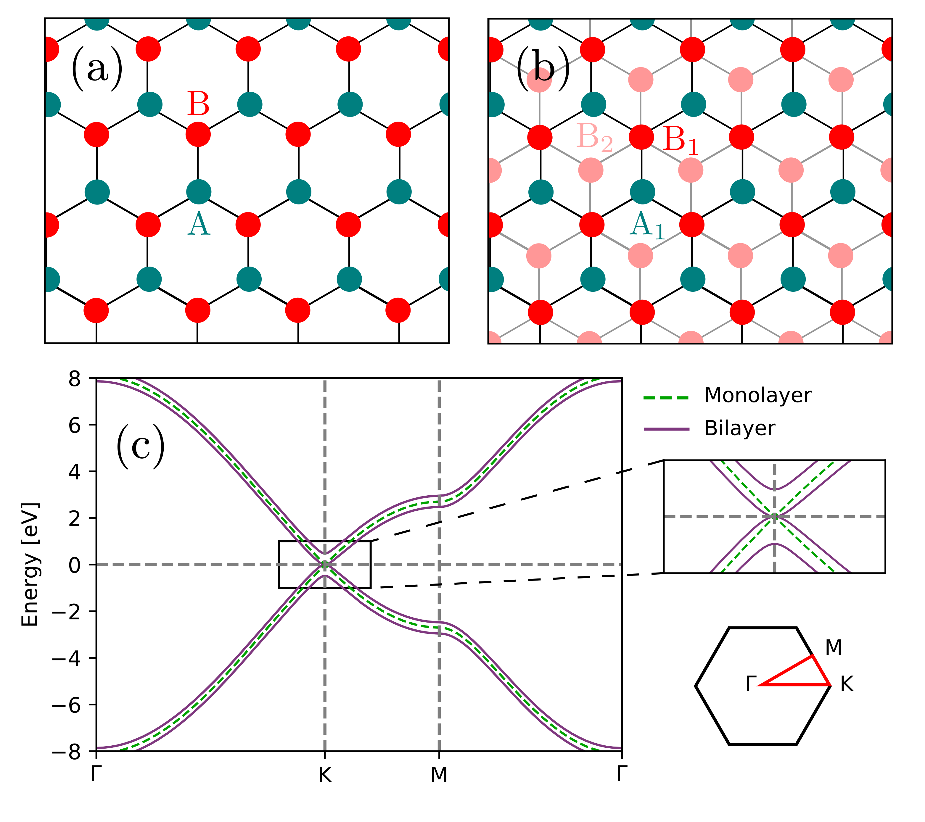
Figure 3.1: Monolayer and bilayer graphene (AB-stacked). The top view of (a) the monolayer and (b) bilayer graphenes, respectively. The carbon atoms are arranged in a honeycomb lattice with two inequivalent carbon atoms (A and B). In bilayer graphene, the B atoms of the top layer are placed on top of A atoms of the bottom layer. (c) The band structure of the monolayer (green) and bilayer graphene (violet).

The real-space lattice of monolayer graphene is shown in Fig. 3.1(a). Carbon atoms are arranged in a honeycomb lattice with a two-atom basis unit-cell. A and B in Fig. 3.1(a) represents two inequivalent carbon atoms in a unit cell. The lattice parameter of graphene is equal to 2.46 Å. Nearest-neighbour tight-binding approximation is implemented by only considering the $p{{}_{z}}$ orbitals of the carbon atoms. The Hamiltonian for monolayer graphene is defined as

$$\hat{\mathcal{H}}_{0}=-t_{0}f(\textbf{k})\hat{a}^{\dagger}_{k}\hat{b}_{k}+\textrm{H.c.}$$ (3.1.1)

Here, $\hat{a}_{k}^{\dagger}$ ($\hat{b}_{k}$) is the creation (annihilation) operator associated with A (B) type of the atom in the unit cell, $f(\textbf{k})$ is defined as $f(\textbf{k})=\sum_{i}e^{i\textbf{k}\cdot\delta_{i}}$, where $\delta_{i}$ is the nearest neighbour vectors. A nearest-neighbour in-plane hopping energy $t_{0}$ of 2.7 eV is used (Reich et al., 2002; Trambly de Laissardière et al., 2010; Moon and Koshino, 2012). The eigenvalues of the Hamiltonian are given by

$$\mathcal{E}(\textbf{k})=\pm t_{0}|f(\textbf{k})|.$$ (3.1.2)

Similarly, the Hamiltonian for AB-stacked bilayer graphene can be defined as

$$\hat{\mathcal{H}}_{AB}=-t_{0}f(\textbf{k})\left[\hat{a}^{\dagger}_{1k}\hat{b}_{1k}+\hat{a}^{\dagger}_{2k}\hat{b}_{2k}\right]+t_{\perp}\hat{a}^{\dagger}_{2k}\hat{b}_{1k}+\textrm{H.c.}$$ (3.1.3)

Here, 1 and 2 denote the carbon atoms in the upper and lower layers, respectively. An inter plane hopping energy $t_{\perp}$ of 0.48 eV is used for an interlayer separation equal to 3.35 Å (Trambly de Laissardière et al., 2010; Moon and Koshino, 2012). The band-structure for the bilayer graphene is given as

$$\mathcal{E}(\textbf{k})=[\pm t_{\perp}\pm\sqrt{4|f(\textbf{k})|^{2}t_{0}^{2}+t_{\perp}^{2}}]/2.$$ (3.1.4)

Figure 3.1(c) presents the energy band-structure of both monolayer and bilayer graphene. The band-structure of monolayer graphene has zero band-gap and linear dispersion near two points, known as $\bf{K}$-points, in the Brillouin zone. On the other hand, bilayer graphene near $\bf{K}$-points shows a quadratic dispersion. Due to the zero band-gap nature, both monolayer and bilayer graphene are semi-metals. Here, electron-hole symmetry is considered by neglecting higher-order hopping and overlap of the orbitals.

SBE in Houston basis is solved (Houston, 1940; Krieger and Iafrate, 1986; Floss et al., 2018) as discussed in section 2.3.1. The momentum matrix elements between $\left|m,\textbf{k}\right\rangle$ and $\left|n,\textbf{k}\right\rangle$ states from the tight-binding Hamiltonian can be obtained as (Pedersen et al., 2001)

$$\textbf{p}_{nm}(\textbf{k})=\left\langle n,\textbf{k}\right|\nabla_{\textbf{k}}\hat{\mathcal{H}}_{\textbf{k}}\left|m,\textbf{k}\right\rangle.$$ (3.1.5)

For HHG from monolayer graphene, a dephasing time within the range of 2 fs to 35 fs has been used in the past (Sato et al., 2021; Liu et al., 2018; Taucer et al., 2017). Moreover, a detailed investigation about dephasing time dependence on HHG from monolayer graphene has been discussed in Ref. (Liu et al., 2018). In this chapter, a dephasing time of 10 fs is considered for monolayer, bilayer, and gapped graphene.

From the harmonic spectrum calculated using Eq. (2.3.11), the integrated yield for $n^{\textrm{th}}$ harmonic in $\mu$-direction can be calculated as

$$\mathcal{I}^{(n)}_{\mu}=\int_{(n-0.5)\omega}^{(n+0.5)\omega}\mathcal{I}_{\mu}(\omega^{\prime})d\omega^{\prime}.$$ (3.1.6)

Ellipticity of the $n^{\textrm{th}}$ harmonic can be calculated from the integrated harmonic yield as

$$|\epsilon_{n}|=\min\left(\leavevmode\nobreak\ \sqrt{\frac{\mathcal{I}^{(n)}_{y}}{\mathcal{I}^{(n)}_{x}}},\sqrt{\frac{\mathcal{I}^{(n)}_{x}}{\mathcal{I}^{(n)}_{y}}}\leavevmode\nobreak\ \right).$$ (3.1.7)

Optical joint density of states (JDOS) estimates the number of available states for an electron to do an interband transition from the valence to conduction band absorbing an energy $E(=E_{c}-E_{v})$. JDOS is calculated as

$${\rm JDOS}(E)=\int\frac{dS}{\left|\nabla_{\textbf{k}}(E_{c}(\textbf{k})-E_{v}(\textbf{k}))\right|}.$$ (3.1.8)

The integral is performed over a constant energy surface with energy $E$ in momentum space.

3.2 Results

In this chapter, a driving laser pulse with an intensity of 1$\times$10¹¹ W/cm² and a wavelength of 3.2 $\mu$m are used. The laser pulse is eight-cycles in duration with a sin-squared envelope. The intensity of the driving pulse is much below the damage threshold and lower than the one used in experimental HHG from graphene (Yoshikawa et al., 2017; Taucer et al., 2017). The same parameters of the driving laser pulse are used throughout this chapter unless stated otherwise.

3.2.1 HHG from Monolayer and Bilayer Graphene

In this section, we discuss HHG from monolayer and bilayer graphene with AA and AB configurations. Moreover, the role of interband and intraband contributions are investigated in both cases. The role of interlayer coupling in HHG from bilayer graphene is investigated. Furthermore, polarisation and ellipticity dependences of the HHG are discussed.

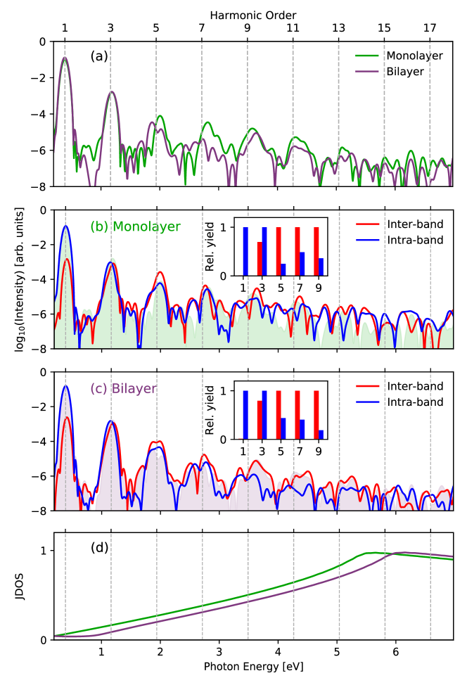
Figure 3.2: (a) High-harmonic spectrum of the monolayer (green) and bilayer (violet) graphene with AB stacking. A linearly polarized pulse along the $\Gamma$-K direction is considered here. The high-harmonic intensity is normalised to the total number of electrons in monolayer and bilayer graphenes. The interband and intraband contributions to the high-harmonic spectrum for (b) monolayer and (c) bilayer graphenes. The total harmonic spectrum is also plotted for the reference. The relative harmonic yield (integrated) for different orders from interband and intraband contributions is plotted in the insets of (b) and (c), respectively. (d) The normalised optical joint density of states (JDOS) of monolayer (green) and bilayer (violet) graphenes.

Figure 3.2 presents the HHG spectrum of monolayer graphene and its comparison with the spectrum of the bilayer graphene for a linearly polarised laser pulse polarised along $x$-axis ($\Gamma$-K in the Brillouin zone). Here, AB stacking of bilayer graphene is considered. The intensity of the HHG spectrum is normalised with respect to the total number of electrons in monolayer and bilayer graphenes. It is apparent that the third harmonic (H3) is matching well in both cases. However, harmonics higher than H3 show significantly different behaviour as the interlayer coupling between the two layers plays a meaningful role.

The interband and intraband contributions to the total harmonic spectra for monolayer and bilayer graphene are shown in Figs. 3.2(b) and (c), respectively. Both contributions play a strong role to the total spectra as reflected from the figure. A strong interplay of interband and intraband contributions was reported for monolayer graphene (Taucer et al., 2017; Liu et al., 2018; Al-Naib et al., 2014). Unlike the wide band-gap semiconductors (Wu et al., 2015), the interband and intraband transitions take place at the same energy scales for both monolayer and bilayer graphenes (Stroucken et al., 2011) due to the vanishing band-gap. The relative (integrated) harmonic yield from interband and intraband contributions is plotted in the insets of Figs. 3.2(b) and (c). Here, intraband contribution dominates upto H3, whereas interband contribution dominates for fifth (H5) and higher-order harmonics for both monolayer and bilayer graphenes. The enhanced contributions from interband transitions at higher orders can be attributed to the increased joint density of states at higher energies as shown in Fig. 3.2(d).

Also, as the low-energy band structures are different for monolayer and bilayer graphenes [Fig. 3.1(c)], the nature of harmonic spectra is not obvious from the band-structure point of view. To have a better understanding of the underlying mechanism of the harmonic generation in both cases, the role of the interlayer coupling in HHG is discussed in the next subsection.

Role of Interlayer Coupling in HHG

To understand how the interlayer coupling between two layers affects the harmonic generation in bilayer graphene, the harmonic spectrum as a function of interlayer coupling strength ($t_{\perp}$) is shown in Fig. 3.3(a). Reducing the interlayer coupling strength is equivalent of moving the two layers of graphene farther apart. The red dashed line in Fig. 3.3(a) corresponds to the interlayer coupling used in simulations presented in Fig. 3.2. It is evident from Fig. 3.3(a) that H5 and higher-order harmonics are sensitive with respect to $t_{\perp}$. Moreover, different harmonic orders affected differently. Therefore, the yield of harmonic orders are non-linear functions of interlayer coupling.

To explore further how different hopping terms affect the HHG in bilayer graphene, an additional hopping term, $t_{3}$, between B atoms of the top layer and A atoms of the bottom layer is introduced. The modified Hamiltonian for AB-stacked bilayer graphene can be written as

$$\begin{split}\hat{\mathcal{H}}_{AB}=&-t_{0}f(\textbf{k})\left[\hat{a}^{\dagger}_{1k}\hat{b}_{1k}+\hat{a}^{\dagger}_{2k}\hat{b}_{2k}\right]\\ &+t_{\perp}\hat{a}^{\dagger}_{2k}\hat{b}_{1k}-t_{3}f^{*}(\textbf{k})\hat{a}^{\dagger}_{1k}\hat{b}_{2k}+\textrm{H.c.}\end{split}$$ (3.2.1)

Here, a hopping energy $t_{3}$ of 0.3 eV is used (Charlier et al., 1991; Min et al., 2007). The corresponding harmonic spectrum is presented in Fig. 3.3(b). It is evident from the figure that the additional interlayer coupling $t_{3}$ affects all the harmonics higher than H3. It is apparent that the interlayer coupling has a strong role in determining the non-linear response of bilayer graphene.

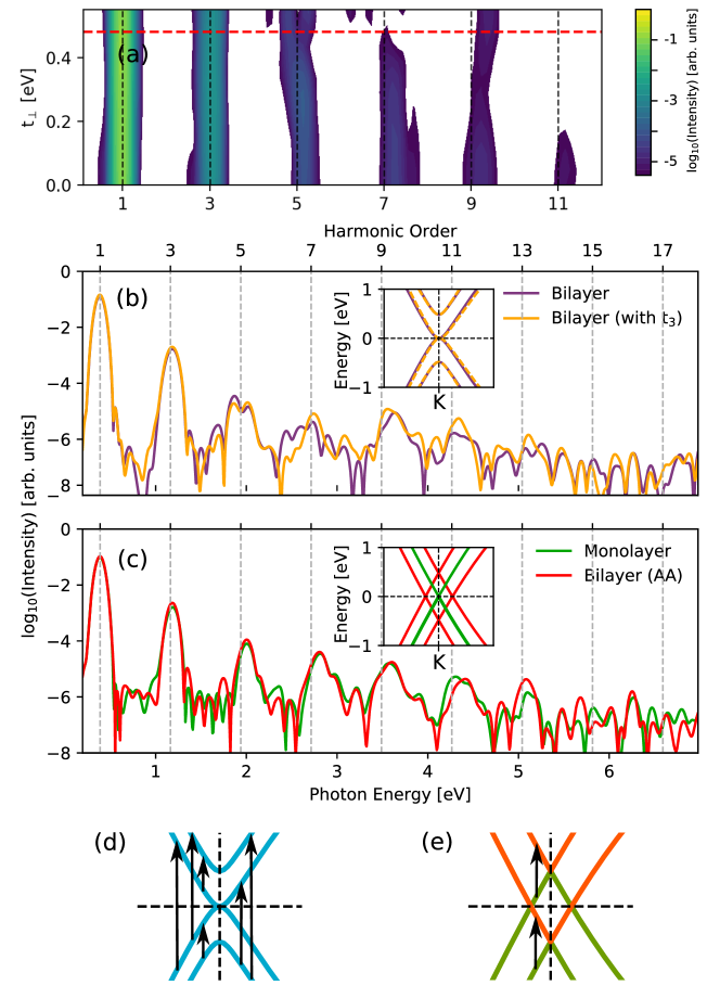
Figure 3.3: (a) High-harmonic spectrum of bilayer graphene with AB stacking as a function of interlayer coupling ($t_{\perp}$), where $t_{\perp}$ = 0 corresponds to the HHG from monolayer graphene. The red dashed line corresponds to the actual value of $t_{\perp}$ used in the calculations. (b) HHG from bilayer graphene (in AB stacking) with $t_{\perp}$ (B₁-A₂) coupling only (violet) and with both $t_{\perp}$ and $t_{3}$ (A₁-B₂) coupling (orange). (c) HHG from bilayer graphene with AA stacking (red) and monolayer graphene (green). In (b) and (c), the band-structures near the $\bf{K}$-point are shown in the inset. (d) and (e) show the non-zero momentum matrix elements in AB and AA stacked bilayer graphene, respectively.

Now let us discuss how HHG depends on different stacking configurations of the bilayer graphene. As discussed in the introduction, bilayer graphene can be realised in AA and AB stacking. AA stacking of bilayer graphene is realised by stacking the monolayer precisely on top of the first layer. The top view of the AA-stacked bilayer looks exactly as a monolayer graphene [Fig. 3.1(a)], where A₁ couples with A₂ and B₁ couples with B₂ with a coupling strength of $t_{\perp}$. The harmonic profile of the bilayer graphene with AA configuration matches well with the spectrum of monolayer graphene as presented in Fig. 3.3(c).

The band structures near the $\bf{K}$-point for AB and AA stacked bilayer graphene are shown in the insets of Figs. 3.3(b) and (c), respectively. For AB-stacked bilayer graphene, a slight change in band-structure results in a significant change in the spectrum [see Fig. 3.3(b)]. On the other hand, for AA-stacked bilayer graphene, the difference in the band-structure is not reflected in the spectrum [see Fig. 3.3(c)].

A better understanding about the HHG mechanism can be deduced by considering the roles of the band structure as well as the interband momentum-matrix elements. The energy bands of the AA-stacked bilayer graphene within nearest neighbour tight-binding approximation are given by

$$\mathcal{E}(\textbf{k})=\pm t_{\perp}\pm t_{0}|f(\textbf{k})|.$$ (3.2.2)

This is equivalent to the shifted energy bands of monolayer graphene by $\pm t_{\perp}$. Also the corresponding momentum matrix elements give non-zero values only for the pairs $t_{\perp}\pm t_{0}|f(\textbf{k})|$ and $-t_{\perp}\pm t_{0}|f(\textbf{k})|$ as shown in Fig. 3.3(e). On the other hand, in AB-stacked bilayer graphene, all pairs of bands have non zero momentum matrix elements near the $\bf{K}$-point as shown in Fig. 3.3(d). The similar band dispersion and JDOS compared to monolayer graphene result in similar harmonic spectrum for AA-stacked bilayer graphene. On the other hand, in bilayer graphene, an electron in the conduction band can recombine to a hole in any of the valence bands near the $\bf{K}$-points as shown in Fig 3.3(d). These different interband channels interfere and therefore generate the resulting harmonic spectrum for the AB-stacked bilayer graphene.

From here onward only bilayer graphene with AB stacking is considered, as the HHG spectra of the monolayer and bilayer graphenes with AA stacking are identical. In the succeeding subsections, we explore polarisation and ellipticity dependences of the HHG from monolayer and bilayer graphenes.

Polarisation-Direction Dependence on the High-Harmonic Spectrum

The vector potential corresponding to a linearly polarised laser pulse can be defined as

$$\textbf{A}(t)=A_{0}f(t)\cos(\omega t)\left[\cos(\theta)\hat{\textbf{e}}_{x}+\sin(\theta)\hat{\textbf{e}}_{y}\right].$$ (3.2.3)

Here, $f(t)$ is the envelope function and $\theta$ is the angle between laser polarisation and the $x$-axis ($\Gamma$-K in the Brillouin zone).

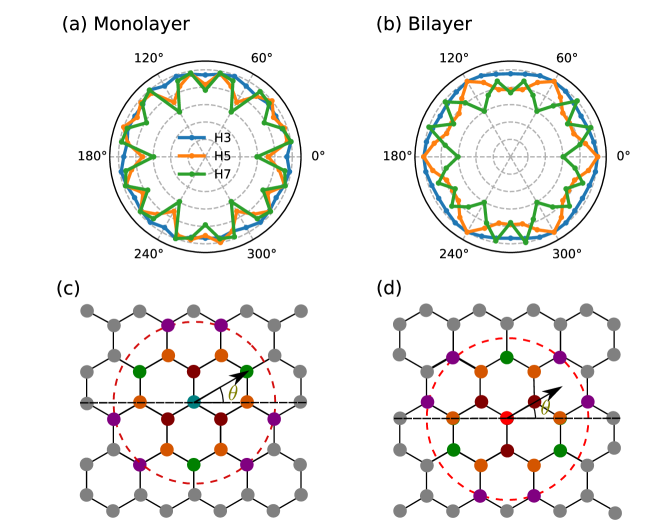
Figure 3.4: Polarisation dependence of the normalised harmonic yield for (a) monolayer and (b) bilayer graphenes. Here, $\theta$ is an angle between laser polarisation and the $x$-axis along $\Gamma$-K in the Brillouin zone. An illustration of the semi-classical real-space model with nearest neighbours of (c) A-type and (d) B-type carbon atoms. The first, second, third, and fourth nearest neighbours are shown using brown, orange, green and violet colours, respectively.

.

Figure 3.5: Polarisation dependence of the normalised harmonic yield for monolayer (top-panel) and bilayer (bottom-panel) graphene. Wavelength values of 2.8 $\mu$m, 3.2 $\mu$m, and 3.6 $\mu$m are used.

.

The polarisation-direction dependence on the harmonic yield for monolayer and bilayer graphenes is presented in Figs. 3.4(a) and (b), respectively. All the harmonics mimic the six-fold symmetry of the graphene lattice. As reflected from the figure, H3 exhibits no significant polarisation sensitivity for both monolayer and bilayer graphenes. The reason for this isotropic nature can be attributed to the isotropic nature of the energy bands near $\bf{K}$-points. However, harmonics higher than H3, show anisotropic behaviour in both cases. Moreover, H5 of monolayer and bilayer graphene shows different polarisation dependence. The harmonic yield is maximum for angles close to 15^∘ and 45^∘ in monolayer graphene.

To understand the polarisation dependence of the harmonic yield in monolayer graphene, we employ a semiclassical explanation as proposed in Refs. (You et al., 2017a; Mrudul et al., 2019) by assuming that the interband transitions can be translated to a semi-classical real-space model (Kruchinin et al., 2018; Parks et al., 2020). One-to-one correspondence between interband transition and inter-atom hopping in graphene was shown by Stroucken et al. (Stroucken et al., 2011). Here, we assume that an electron can hop between two atoms when the laser is polarised along a direction in which it connects the atoms. The contributions to the harmonic yield from different pairs of atoms drop significantly as the distance between the atoms increases. This is in principle governed by the inter-atom momentum matrix elements (Stroucken et al., 2011). By assuming a finite radius for atoms, farther atoms show sharper intensity peaks as a function of angle of polarisation.

Figures 3.4(c) and (d) show the nearest neighbours of A and B types of atoms in the unit cell, respectively. Brown, orange, green and violet coloured atoms are first, second, third and fourth neighbours, respectively. By only considering the nearest-neighbour hopping in graphene, we can see that the maximum yield should be for 30^∘ (along $\Gamma$-M direction). However, the maximum yield is near 15^∘ and 45^∘ as seen from Fig. 3.3(a). This means that the contributions up to the fourth nearest neighbours should be considered to explain the polarisation dependence of H5 and seventh harmonic (H7) of monolayer graphene.

In bilayer graphene, H7 follows the same qualitative behaviour as that of H5 and H7 of monolayer graphene [Fig. 3.3(b)]. In contrast, H5 shows different behaviour and obeys the symmetry of the second nearest neighbour. It is clear from Fig. 3.3(d) that there are multiple paths for interband transitions for bilayer graphene. In bilayer graphene, interband transitions from different pairs of valence and conduction bands can contribute to a particular harmonic, and these different transitions interfere. This makes the mechanism of harmonic generation from monolayer and AB-stacked bilayer graphene different.

It is important to point out that the polarisation dependence is sensitive to the wavelength of driving laser pulse. We present the polarisation-dependence for laser pulses of wavelengths of 2.8 $\mu$m, 3.2 $\mu$m, and 3.6 $\mu$m in Fig. 3.5. For longer wavelengths, electron dynamics occurs in the isotropic parts of the reciprocal space (close to $\mathbf{K}$-points), and as a result the harmonic spectrum can be entirely isotropic. We have confirmed that the different symmetry observed for monolayer and bilayer graphene is compatible with varying wavelength of the driving laser, and our explanation remains consistent.

Ellipticity Dependence on the High-Harmonic Spectrum

The high-harmonic spectra for monolayer and bilayer graphenes corresponding to different polarisation of the driving laser pulse are shown in Fig. 3.6. The vector potential corresponding to the elliptically polarised pulse with an ellipticity $\epsilon$ is defined as

$$\textbf{A}(t)=\frac{A_{0}f(t)}{\sqrt{1+\epsilon^{2}}}\left[\cos(\omega t)\hat{\textbf{e}}_{x}+\epsilon\sin(\omega t)\hat{\textbf{e}}_{y}\right].$$ (3.2.4)

Here, the same laser parameters are used as mentioned in Section 3.2. Both monolayer and bilayer graphenes show significant ellipticity-dependence in the harmonic yield. A negligible harmonic yield is obtained for circularly polarised laser pulse. This indicates that using a single colour mid-infrared circular driver is not an appropriate method to generate circularly polarised harmonics from graphene. This has already been experimentally demonstrated (Taucer et al., 2017; Yoshikawa et al., 2017). Recent theoretical studies revealed that efficient generation of circularly polarised harmonics is possible from graphene either by using a near-infrared circular laser pulse (Chen and Qin, 2019) or by using mid-infrared bi-circular counter-rotating laser pulses (Mrudul et al., 2021). The harmonic spectrum corresponding to bilayer graphene shows the ($6n\pm 1$) harmonic orders for circularly polarised laser, as expected from the symmetry considerations (Gupta et al., 2003). To have a better understanding about the variation of the harmonics as a function of ellipticity of the driving laser, we show the integrated harmonic yield below.

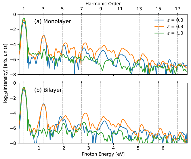
Figure 3.6: High-harmonic spectrum for (a) monolayer and (b) bilayer graphenes for different ellipticities of the driving laser pulse. Here, $\epsilon$ = 0 corresponds to a linearly polarised pulse and $\epsilon$ = 1 corresponds to a circularly polarised pulse.

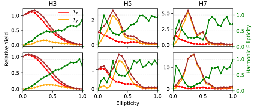
Figure 3.7: Ellipticity dependence of the integrated harmonic yield for 3${}^{\textrm{rd}}$ (H3), 5${}^{\textrm{th}}$ (H5), and 7${}^{\textrm{th}}$ (H7) harmonics of the monolayer (top panel) and bilayer graphenes (bottom panel). The integrated harmonic yield, and its $x$ and $y$-components are shown by brown, red and orange colour lines, respectively. The green line shows the ellipticity dependence on the averaged ellipticity of the emitted harmonics. An elliptically polarised pulse with an intensity of 1$\times$10¹¹ W/cm² is used for HHG.

The harmonic yield as a function of ellipticity for the monolayer (top panel) and bilayer graphenes (bottom panel) are presented in Fig. 3.7. The total harmonic yield is normalised with respect to the harmonic yield for $\epsilon$ = 0. The ellipticity dependence of all the three harmonics agrees qualitatively well for monolayer and bilayer graphenes. The atomic-like ellipticity dependence of H3 can be attributed to its isotropic nature [see first column of Fig. 3.7 ]. However, H5 and H7 show a characteristic ellipticity dependence. The harmonic yield has a maximum for a finite value of the ellipticity and is polarised along the normal direction of the major axis of the ellipse. This interesting feature was observed for the monolayer graphene experimentally and explained as a consequence of the semi-metallic nature of the monolayer graphene (Yoshikawa et al., 2017). Since bilayer graphene is also semi-metallic, it is also expected to exhibit similar ellipticity dependence, which we confirm here.

The different qualitative behaviours of the ellipticity dependence of H3 compared to H5 and H7 are also consistent with the findings that the interband and intraband mechanisms respond differently to the ellipticity of the driving laser (Tancogne-Dejean et al., 2017a) [see also insets of Figs. 3.2(b) and (c)]. The characteristic ellipticity dependence of monolayer graphene was shown to be dominated by interband contributions in Ref. (Liu et al., 2018). The ellipticity of the maximum yield is different for bilayer graphene as a consequence of interlayer coupling.

The averaged ellipticity of the emitted harmonics as a function of the laser ellipticity shows interesting behaviour as shown in Fig. 3.7 (see green colour). The averaged ellipticity of H3 of monolayer and bilayer graphene shows monotonically increasing behaviour. On the other hand, the behaviour is highly nonlinear for harmonics higher than H3. It is also interesting to note that harmonics with higher ellipticity can be obtained by a nearly linearly polarised pulse ($\epsilon<$0.3).

3.2.2 HHG from Gapped Graphene

The Hamiltonian for gapped graphene can be modelled by adding different onsite energy at A and B sublattices of graphene [see Fig. 3.1(a)]. Equation (3.1.1) modifies as

$$\hat{\mathcal{H}_{g}}=-t_{0}f(\textbf{k})a_{k}^{\dagger}b_{k}-\frac{\Delta_{g}}{2}a_{k}^{\dagger}a_{k}+\frac{\Delta_{g}}{2}b_{k}^{\dagger}b_{k}+\textrm{H.c.}$$ (3.2.5)

Here, $\Delta_{g}$ is the minimum band-gap energy at $\mathbf{K}$-points in the Brillouin zone. The energy eigenvalues of the gapped graphene are given by

$$\mathcal{E}(\textbf{k})=\pm\sqrt{(\Delta_{g}/2)^{2}+t_{0}^{2}|f(\textbf{k})|^{2}}.$$ (3.2.6)

Adding a small energy gap essentially breaks the inversion symmetry of the lattice. This means that A and B atoms in Fig. 3.1(a) represent entirely different atoms in this model. An example of such a system is monolayer h-BN.

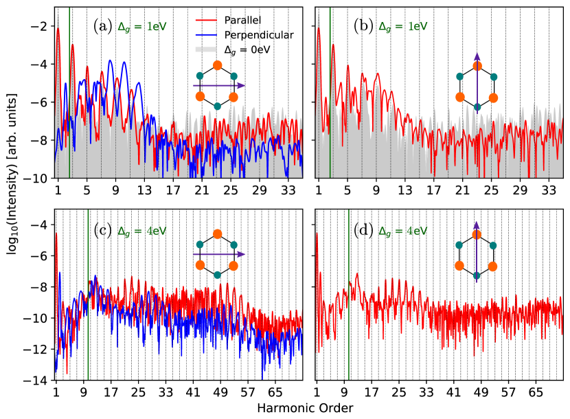
Figure 3.8: High-harmonic spectrum of gapped graphene with $\Delta_{g}$ = 1 eV [(a), (b)], and $\Delta_{g}$ = 4 eV [(c), (d)]. The green vertical line shows the band gap of the gapped graphene. The laser polarisation is along the $x$-axis in (a) and (c), and along the $y$-axis in (b) and (d). Red and blue lines show the harmonic signal parallel and perpendicular to the laser polarisation, respectively. The grey shaded region in (a) and (b) are the harmonic spectra for gapless graphene.

In this section, we use the same laser parameters as mentioned in the previous section. A driving laser pulse with an intensity of 1$\times$10¹¹ W/cm² and a wavelength of 3.2 $\mu$m are used. The laser pulse has eight-cycles in duration with a sin-squared envelope.

The harmonic spectra corresponding to gapped graphene are presented in Fig. 3.8. Here, $\Delta_{g}$ values of 1 eV [Fig. 3.8(a), (b)] and 4 eV [Fig. 3.8(c), (d)] are considered. The left (right) panel of Fig. 3.8 shows the spectra calculated when the laser is polarised along the $x$-axis ($y$-axis). Here, the mirror plane of the crystal is along the $y$-axis (see inset of Fig. 3.8).

There is a stronger polarisation direction dependence in gapped graphene as evident from figure. Both even and odd harmonics are present in the harmonic spectrum. Even harmonics are generated perpendicular to the laser field when the laser is polarised along the $x$-axis. On the other hand, even and odd harmonics are generated parallel to the laser field when the laser is along the $y$-axis. Moreover, for $\Delta_{g}=1$ eV, the odd harmonics spectrum is comparable to the HHG spectrum for gapless graphene [see Fig. 3.2 (a)]. In contrast, for $\Delta_{g}=4$ eV, the intensity of the harmonics are decreased by at least two orders, and the characteristics of the harmonic spectrum are changed drastically.

Figure 3.9: (a) Second-harmonic (H2) generated from gapped graphene ($\Delta_{g}$ = 4 eV). The laser polarisation is along the $x$-axis for blue line (see Fig. 3.8(c)), and along the $y$-axis for orange line [see Fig. 3.8(d)]. (b) Integrated conduction-band population during the laser pulse.

The point group symmetry is reduced from $\mathbf{D}_{6h}$ to $\mathbf{D}_{3h}$ in gapped graphene as inversion symmetry is broken. As a consequence, we see even harmonics in the spectrum. Here, we present the symmetry of the second-order nonlinear susceptibility of gapped graphene to understand the selection rules for even harmonics. For any material, the contributions from the second-order nonlinear susceptibility tensor $\chi^{(2)}_{\mu\nu\lambda}$ to the polarisation is given by

$$P_{\mu}^{(2)}=\sum_{\nu,\lambda}\chi^{(2)}_{\mu\nu\lambda}\mathcal{F}_{\nu}\mathcal{F}_{\lambda}.$$ (3.2.7)

Here, $\mathcal{F}_{\mu}$ is the electric field in the $\mu$-direction. For a material with inversion symmetry, all elements of the $\chi^{(2)}$ tensor is supposed to be zero. In contrast, for a material without inversion symmetry, the non-zero elements of $\chi^{(2)}$ are dictated by the corresponding point group symmetry. For $\mathbf{D}_{3h}$ point group, non-zero elements of $\chi^{(2)}$ hold the following relation: $\chi^{(2)}_{yyy}$ = -$\chi^{(2)}_{yxx}$ = $\chi^{(2)}_{xxy}$ = -$\chi^{(2)}_{xyx}$ (Boyd, 2020). When the laser is polarised along the $x$-axis, contribution to the polarisation vector (dipole moment per unit volume) from $\chi^{(2)}$ is given by $P_{y}^{(2)}=\chi^{(2)}_{yxx}\mathcal{F}_{x}\mathcal{F}_{x}$. Similarly, for a laser polarised along the $y$-axis, $P_{y}^{(2)}=\chi^{(2)}_{yyy}\mathcal{F}_{y}\mathcal{F}_{y}$. These clearly explain the selection rules of even harmonics in gapped graphene for a linearly polarised electric field. To further support our claim, it is expected from $\chi^{(2)}_{yyy}=-\chi^{(2)}_{yxx}$ that the resultant second harmonic is $y$-polarised but differ by a sign for laser polarised along $x$- and $y$-directions. This claim is established by presenting the second harmonic for $x$- and $y$-polarised laser in Fig. 3.9(a).

We present the integrated conduction-band population during the laser to examine the electron dynamics in gapped graphene in Fig. 3.9(b). The conduction band population decreases drastically as the gap increases. Clearly, the interband electron transitions are diminished in gapped graphene. This is also the reason for the less intense harmonic spectrum of gapped graphene [see Fig. 3.8(c)-(d)].

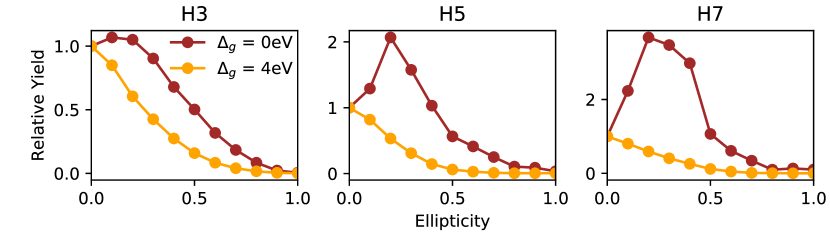
Figure 3.10: Ellipticity dependence on the integrated harmonic yield for 3${}^{\textrm{rd}}$ (H3), 5${}^{\textrm{th}}$ (H5), and 7${}^{\textrm{th}}$ (H7) harmonics of gapless (brown) and gapped (orange) graphene. The laser is polarised along $x$-axis.

We can see clean or noisy harmonics in different parts of the harmonic spectrum. The reason can be understood as follows: both interband and intraband current contribute to the harmonic spectrum and their interference results in noisy harmonics. When one of the channels is suppressed, we get clean harmonics (Tancogne-Dejean et al., 2017b). For example, in the below bandgap regime, only intraband dynamics are possible, resulting in clean harmonics in this regime.

Ellipticity dependence on the integrated harmonic yield of gapped ($\Delta_{g}$ = 4 eV) and gapless graphene are presented in Fig. 3.10. Unlike monolayer or bilayer graphene (see Fig. 3.7), the low-order harmonics lack anomalous ellipticity dependence in gapped graphene. This further supports the claim that this feature in gapless graphene originates from the semi-metallic nature of strong field interaction (Yoshikawa et al., 2017). Moreover, we have discussed the significance of interband current on the anomalous ellipticity dependence of gapless graphene in Section 3.2.1. On the other hand, the ellipticity dependence on the low-order harmonics of gapped-graphene originates entirely from intraband dynamics, resulting in atom-like ellipticity dependence.

Gapped graphene has non-zero Berry curvature as a consequence of inversion symmetry breaking. The velocity of an electron in $n^{\textrm{th}}$ energy band is given by

$$\textbf{v}_{n}(\textbf{k})=\nabla_{\textbf{k}}\mathcal{E}_{n}(\textbf{k})-\mathcal{F}(t)\times\Omega_{n}(\textbf{k}).$$ (3.2.8)

The first term on the right originates from the band-dispersion and the second term stems from the Berry curvature $\Omega_{n}$. This semiclassical electron dynamics in a particular band is directly linked to the intraband current. This means that the perpendicular even harmonics in Fig.3.8(a), (c) arise from the material’s Berry curvature. In our calculation, the diagonal elements of the dipole matrix elements, $\textbf{d}_{mn}$ gives the Berry connection, i.e., $\mathcal{A}_{n}(\textbf{k})=\textbf{d}_{nn}(\textbf{k})=i\left\langle u_{n,\textbf{k}}|\nabla_{\textbf{k}}|u_{n,\textbf{k}}\right\rangle$. Berry curvature and Berry connection are related as $\Omega_{n}(\textbf{k})=\nabla_{\textbf{k}}\times\mathcal{A}_{n}(\textbf{k})$. Harmonic spectrum with and without Berry connection is presented in Fig. 3.11. It is evident that exclusion of Berry connection affects HHG spectrum considerably and the difference is strong near and below the band-gap energy region. This can be attributed to the fact that Berry curvature affects the intraband current.

Figure 3.11: High-harmonic spectrum of gapped graphene with and without including Berry curvature. The laser polarisation is along the $x$-axis.

3.3 Summary

In summary, HHG from monolayer, bilayer, and gapped graphenes is discussed. Bilayer graphene having AA and AB stacking are considered in this chapter. The harmonic spectra of the monolayer and bilayer graphenes are significantly different and exhibit characteristic features of having a vanishing band-gap. The HHG spectrum of the bilayer graphene shows signatures of the interlayer coupling, which affects high-order harmonics non-linearly and different harmonics are affected differently. The role of interlayer coupling was also found to be stacking dependent, resulting in a similar harmonic spectrum for monolayer and bilayer graphenes with AA stacking. A strong interplay of the interband and intraband contributions to the total harmonic spectrum is noticed. Moreover, distinct polarisation and ellipticity dependence are observed in monolayer and bilayer graphenes. The harmonic spectrum of gapped graphene is significantly different from gapless graphene. Breaking inversion symmetry results in even harmonics, and the selection rules can be explained using the point group symmetry of the material. The polarisation and ellipticity dependence is significantly different in gapless and gapped graphene. We also show the significance of Berry curvature in the harmonic spectrum of gapped graphene.

Chapter 4 Light-induced Valleytronics in Pristine graphene

One of the most interesting features of graphene and gapped graphene materials is the electron’s extra degree of freedom, the valley pseudospin, associated with populating the local minima $\mathbf{K}$ and $\mathbf{K}^{\prime}$ in the lowest conduction band of the Brillouin zone. This extra degree of freedom has the potential to encode, process and store quantum information, opening the field of valleytronics (Vitale et al., 2018).

The monolayer graphene, as opposed to gapped graphene materials, presents a fundamental challenge for valleytronics: it has zero band-gap and zero Berry curvature. These aspects are generally considered to be a major impediment for valleytronics. In gapped graphene materials, valley selectivity is achieved by matching the helicity of a circularly polarized pump pulse, resonant to the band gap, to the sign of the Berry curvature (Schaibley et al., 2016; Mak et al., 2012; Jones et al., 2013; Gunlycke and White, 2011; Xiao et al., 2012). Recently demonstrated (Langer et al., 2018) sub-cycle manipulation of electron population in $\mathbf{K}$ and $\mathbf{K}^{\prime}$ valleys of tungsten diselenide, achieved with the combination of a resonant pump pulse locked to the oscillations of the THz control pulse, represents a major milestone. Precise sub-cycle control over the driving light fields opens new opportunities for valleytronics, such as those offered by the new concept of a topological resonance, discovered and analysed in Refs. (Motlagh et al., 2019a, 2018; Kelardeh et al., 2016). Single-cycle pulses with the controlled phase of carrier oscillations under the envelope offer a route to valleytronics in gapped graphene-type materials even when such pulses are linearly, not circularly, polarized (Jiménez-Galán et al., 2021). It is also possible to avoid the reliance on resonances in gapped graphene-type materials, breaking the symmetry between the $\mathbf{K}$ and $\mathbf{K}^{\prime}$ valleys via a light-induced topological phase transition, closing the gap in the desired valley (Jiménez-Galán et al., 2020).

Thus, with its zero band-gap, zero Berry curvature, and identical dispersion near the bottom of the valleys, pristine graphene appears unsuitable for valleytronics – a disappointing conclusion in view of its exceptional transport properties. In this chapter, we discuss how this generally accepted conclusion is not correct, and that the preferential population of a desired valley can be achieved by tailoring the polarization state of the driving light pulse to the symmetry of the lattice. Present proposal offers an all-optical route to valleytronics in pristine graphene, complementing approaches based on creating a gap by using a heterostructure of graphene with hexagonal boron nitride (Gorbachev et al., 2014; Yankowitz et al., 2012; Hunt et al., 2013; Rycerz et al., 2007), or by adding strain and/or defect engineering (Grujić et al., 2014; Settnes et al., 2016; Faria et al., 2020; Xiao et al., 2007).

We also show valley selectivity of harmonic generation in graphene and demonstrate it with the same field as we use for valley-selective electronic excitation. This aid us to understand how the underlying electron dynamics are different. Last but not least, we describe an all-optical method for measuring valley-polarisation in graphene with a weak probe-pulse.

The key idea of our approach is illustrated in Fig. 4.1, which shows graphene in real (a) and reciprocal (b) space, together with the structure of the incident electric field (a) and the corresponding vector potential (b). The field is made by superimposing two counter-rotating circularly polarized colours at the frequencies $\omega$ and $2\omega$. The Lissajous figure for the total electric field is a trefoil, and its orientation is controlled by the relative two-colour phase $\phi$, i.e., the sub-cycle two-colour delay measured in terms of $\omega$. In the absence of the field, the two carbon atoms A and B, in real space, are related by the inversion symmetry. When the field is turned on, this inversion symmetry is broken: the electric field in Fig. 4.1(a) always points from the atom A to the one of the three neighbouring atoms B during the full laser cycle, but not the other way around. If the centre of the Lissajous figure is placed on the atom B, the field points in the middle between its neighbours. One can control this symmetry breaking by rotating the trefoil, interchanging the roles of the atoms A and B. Thus, the bi-circular field offers a simple, all-optical, ultrafast tool to break the inversion symmetry of the graphene lattice in a controlled way. Such controlled symmetry breaking naturally controls the relative excitation probabilities induced by the same laser field in the adjacent $\mathbf{K}$ and $\mathbf{K}^{\prime}$ valleys of the Brillouin zone.

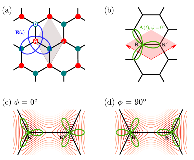
Figure 4.1: (a) Graphene lattice in the coordinate-space, with the Lissajous figure of the bicircular electric field breaking the symmetry between otherwise identical carbon atoms A and B; two-colour phase $\phi=0^{\circ}$. (b) Optically induced symmetry breaking viewed in the momentum space, the vector potential of the bicircular field is shown for $\phi=0^{\circ}$. (c, d) Close-up images of the valleys show their asymmetry, leading to different laser-driven dynamics and different excitation rates once the electron leaves the bottom of the valley. Here, the red contours show the conduction band energy in the reciprocal space.

Figure 4.1(b) provides the complementary reciprocal-space perspective. In the laser field, the electron crystal momentum follows ${\bf k}(t)={\bf k}_{i}+\mathcal{A}(t)$, where ${\bf k}_{i}$ is the initial crystal momentum and $\mathcal{A}(t)$ is the vector potential, shown in Fig. 4.1(b) for the electric field shown in Fig. 4.1(a). The asymmetry between the two valleys with respect to the vector potential is immediately visible.

Figures 4.1(c) and 4.1(d) provide additional support to this qualitative picture. One can observe that the two field-free valleys, $\mathbf{K}$ and $\mathbf{K}^{\prime}$, are only identical near their very bottoms. As soon as one moves away from the bottom, the valleys start to develop the trefoil structure, with $\mathbf{K}$ and $\mathbf{K}^{\prime}$ being the mirror images of each other. How the symmetry of the vector potential fits into the symmetry of the valley away from their bottoms will control the dynamics and the excitation probability.

In sufficiently strong fields, excitation happens not only at the Dirac point where the gap is equal to zero, but also in its vicinity. For the vector potential in Fig. 4.1(c), the average gap seen by the electron when following the vector potential from the Dirac point in the ${\bf K}$ valley, i.e., moving along the trajectory ${\bf K}+\mathcal{A}(t)$, is less than in the $\mathbf{K}^{\prime}$ valley, i.e., when following the trajectory $\mathbf{K}^{\prime}+\mathcal{A}(t)$. In sufficiently strong and low-frequency fields, such that the band gap along the trajectories ${\bf K}+\mathcal{A}(t)$ and $\mathbf{K}^{\prime}+\mathcal{A}(t)$ quickly exceeds the photon energy, the excitation probability should therefore be higher in Fig. 4.1(c). For the same reason, rotating the vector potential as shown in Fig. 4.1(d) should favour population of the $\mathbf{K}^{\prime}$ valley. Here, “quickly" means “within a fraction of one-third of the laser cycle", which is relevant time-scale for the bicircular field. In this context lower laser frequencies leading to higher vector-potential are best suited to meet this requirement

4.1 Numerical Methods

In the simulations, we used the nearest-neighbour tight-binding approximation to obtain the ground state of graphene with a hopping-energy of 2.7 eV (Reich et al., 2002). The lattice parameter of graphene is chosen to be 2.46 Å. The resultant band-structure has zero band-gap with linear dispersion near the two points in the Brillouin zone known as $\mathbf{K}$ and $\mathbf{K}^{\prime}$ points as shown in Fig. 3.1. The density matrix approach was used to follow the electron dynamics in graphene. Time-evolution of density matrix element, $\rho^{\textbf{k}}_{mn}$, was performed using SBE within the Houston basis $|n,\textbf{k}+\mathcal{A}(t)\rangle$ (Golde et al., 2008; Floss et al., 2018), as discussed in Chapter 2 [see Eq. (2.3.9)]. We sampled the Brillouin zone with a 180$\times$180 k-point grid. SBE is solved using fourth-order Runge-Kutta method with a time-step of 0.8 a.u.

4.2 Results and Discussion

The valley-selective electron-dynamics under the tailored field is confirmed by our numerical simulations. In the simulations, graphene is exposed to the bicircular field with the vector potential

$$\mathcal{A}(t)=\frac{A_{0}f(t)}{\sqrt{2}}\left(\left[\cos(\omega t+\phi)+\frac{\mathcal{R}}{2}\cos(2\omega t)\right]\hat{\textbf{e}}_{x}+\left[\sin(\omega t+\phi)-\frac{\mathcal{R}}{2}\sin(2\omega t)\right]\hat{\textbf{e}}_{y}\right).$$ (4.2.1)

Here, $A_{0}=F_{\omega}/\omega$ is the amplitude of the vector potential for the fundamental field, $F_{\omega}$ is its strength, $f(t)$ is the temporal envelope of the driving field, $\phi$ is the sub-cycle phase difference between the two fields, and $\mathcal{R}$ is the ratio of the electric field strengths for the two fields, leading to $\mathcal{R}/2$ ratio for the amplitudes of the vector potentials. The amplitude of the fundamental field was varied up to $F_{\omega}$ = 15 MV/cm, leading to the maximum fundamental intensity 3$\times$10¹¹ W/cm², with the fundamental wavelength $\lambda=6\leavevmode\nobreak\ \mu$m. This laser intensity is weaker than the one used in experiments for monolayer graphene (Yoshikawa et al., 2017; Heide et al., 2018; Higuchi et al., 2017) and is below the damage threshold. We have also varied $\mathcal{R}$, using $\mathcal{R}=1$ and $\mathcal{R}=2$. A pulse duration of 145 femtosecond with sin-square envelope is employed in this work. Our findings are valid for a broad range of wavelengths and field intensities. To obtain the total population of the different valleys, we have integrated the momentum-resolved population over the sections shown in Fig. 4.2(a).

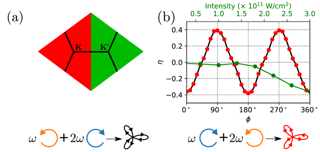
Figure 4.2: (a) Separation of the Brillouin zone into the $\mathbf{K}$ and $\mathbf{K}^{\prime}$ valleys. (b) Asymmetry in the valley-resolved populations in the conduction band as a function of $\phi$ (black line with an intensity 3$\times$10¹¹ W/cm²), and laser intensity (yellow line with $\phi=0^{\circ}$) for a laser with wavelength of 6 $\mu$m, $\mathcal{R}$ = 2, and a dephasing time $T_{2}$ of 10 $fs$. The red dots show the asymmetry as a function of $\phi$ after switching the helicities of both the fields as shown in the bottom panel.

4.2.1 Light-Induced Valley-Polarisation

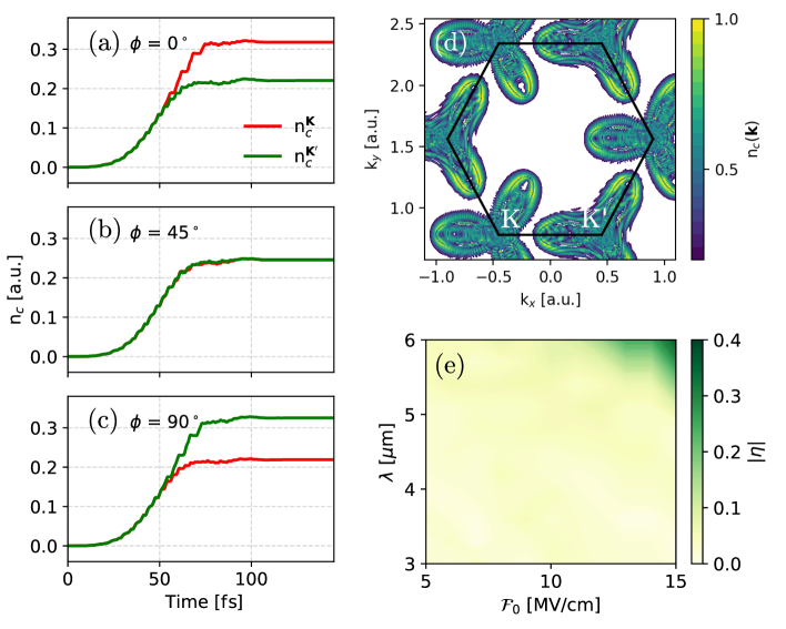
Figure 4.3: (a)-(c) Excitation dynamics during the laser pulse, respectively, for $\phi$ = 0^∘, 45^∘, and 90^∘. (d) Conduction-band population in the Brillouin zone at the peak of the laser pulse. (e) Valley-asymmetry as a function of wavelength ($\lambda$) and electric-field amplitude ($\mathcal{F}_{0}$).

To quantify the amount of the valley polarisation, the valley asymmetry parameter is defined as

$$\eta=\frac{n_{c}^{\mathbf{K}^{\prime}}-n_{c}^{\mathbf{K}}}{(n_{c}^{\mathbf{K}^{\prime}}+n_{c}^{\mathbf{K}})/2},$$ (4.2.2)

where $n_{c}^{\mathbf{K}}$ and $n_{c}^{\mathbf{K}^{\prime}}$ are electron populations at the end of the laser pulse in the conduction band around $\mathbf{K}$ and $\mathbf{K}^{\prime}$ valleys, respectively.

Figure 4.2(b) shows the asymmetry in the populations of the ${\bf K}$ and $\mathbf{K}^{\prime}$ valleys as a function of the two-colour phase $\phi$ (black line), for different values of the fundamental field amplitude and $\mathcal{R}=2$. Substantial contrast between the two valleys is achieved with values as high as $\pm 36\%$ for $\phi=0^{\circ},90^{\circ}$, and no asymmetry for $\phi=45^{\circ}$. Here, each 180^∘ change in $\phi$ results in a 120^∘ rotation of the trefoil, resulting in an equivalent configuration. This is the reason for the two-fold symmetry of the valley-asymmetry in Fig. 4.2(b). The same results are obtained when the helicities of both driving fields are exchanged simultaneously [see red dots in Fig. 4.2(b)].

The higher-populated valley is the one where the vector potential “fits” better into the shape of the valley, minimizing the band gap along the electron trajectory in the momentum space. The asymmetry in the valley population is negligible up to an intensity of $2\times 10^{11}$ W/cm² and gradually increases with intensity [see green line in Fig. 4.2(b)].

To further explore the underlying mechanism, we show the excitation dynamics for three different cases in Figs. 4.3(a)-(c). Analysing Figs. 4.3(a)-(c) along with Fig. 4.2(b) suggests that the valley asymmetry is observed only when the laser pulse is able to drive the electrons to the anisotropic part of the conduction band. We notice that the valley-excitation dynamics is reversed for $\phi$ = 0^∘ and $\phi$ = 90^∘. Since the electron-dynamics in both the valleys are equivalent for $\phi$ = 45^∘, there is no valley-polarisation. The $\bf{k}$-resolved excitation dynamics for $\phi$ = 0^∘ is presented in Fig. 4.3(d). The populations near the valleys show signatures of energy contours [Fig. 4.1(c)] of the respective valley. Figure 4.3(e) shows wavelength and electric-field amplitude dependence on the valley-asymmetry. A reasonable valley asymmetry is achieved for longer wavelengths and stronger electric-field amplitudes. This is directly linked to the fact that the extend an electron travel in the reciprocal space is proportional to the amplitude of the vector-potential, as a consequence of the acceleration theorem.

4.2.2 Valley-Polarised HHG

Figure 4.4(a) shows polarisation-resolved high-harmonic spectrum. The $(3n+1)$ harmonics follow the polarisation of the $\omega$ pulse (left-handed circular polarisation), whereas $(3n+2)$ harmonics follow the polarisation of the $2\omega$ pulse (right-handed circular polarisation), while $3n$ harmonics are missing, just like in atomic media (Fleischer et al., 2014; Neufeld et al., 2019; Dixit et al., 2018; Ansari et al., 2021). In this context, we note that while harmonic generation with single-colour circularly polarized drivers is forbidden in atoms, such selection rules do not generally arise in solids (Ghimire et al., 2011a). However, the ellipticity-dependence studies on graphene show very weak harmonic yield for drivers with higher ellipticity (Yoshikawa et al., 2017; Taucer et al., 2017; Liu et al., 2018), as we have also observed and discussed in the previous chapter. As in atoms, application of bicircular fields allows for efficient generation of circularly polarized harmonics in graphene.

In general, the interband and intraband harmonic emission mechanisms in graphene are coupled (Taucer et al., 2017; Liu et al., 2018; Al-Naib et al., 2014), except at low electric fields (Al-Naib et al., 2014), leading to a complex interplay between the interband and intraband emission mechanisms. We present the interband and intraband resolved HHG spectrum in Fig. 4.4(b). In the present case, the intraband mechanism show dominancy. This further supports our analysis based on the acceleration theorem, which is based on intraband electron dynamics.

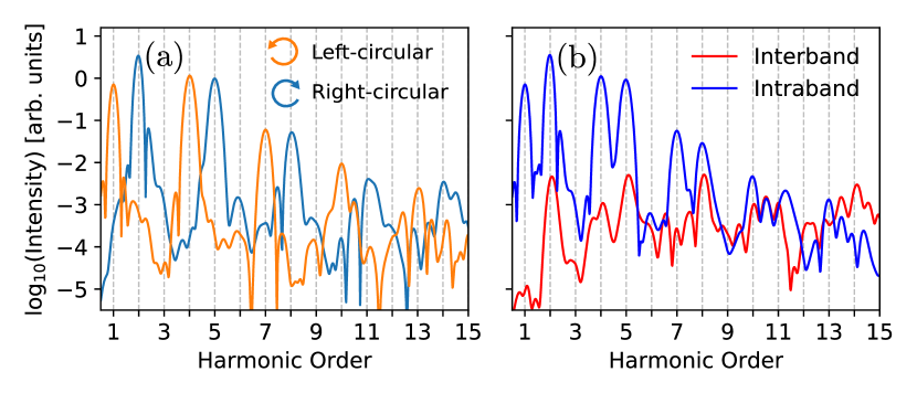
Figure 4.4: (a) Polarisation-resolved high-harmonic emission, for left-handed circularly polarised fundamental (orange) and right-handed circularly polarised second harmonic (blue). Alternating harmonics follow alternating helicities: $3n+1$ follow the fundamental, $3n+2$ follow the second harmonic, the $3n$ harmonics missing due to symmetry. (b) Harmonic spectrum resolved into interband and intraband contributions ($\phi=0^{\circ}$).

The current generated by the electron injection into the conduction band valleys is accompanied by harmonic radiation and makes substantial contribution to the lower-order harmonics, such as H4 and H5 for our two-colour driver. These harmonics are stronger whenever the dispersion $\epsilon({\bf k})$ is more nonlinear. In this respect, for the electrons following the trajectories ${\bf K}+\mathcal{A}(t)$ and $\mathbf{K}^{\prime}+\mathcal{A}(t)$, the current-driven HHG from the $\mathbf{K}^{\prime}$ valley is preferred for the vector potential in Fig. 4.1(c). Conversely, for the vector potential shown in Fig. 4.1(d) low-order, current-driven harmonic generation should be preferred from the ${\bf K}$ valley. Indeed, following the vector potential, the electron is driven against the steeper walls in the $\mathbf{K}^{\prime}$ valley in Fig. 4.1(c) and against the steeper walls in the ${\bf K}$ valley in Fig. 4.1(d).

These qualitative expectations are also confirmed by our numerical simulations, shown in Fig. 4.5. The same laser parameters used in Fig. 4.2 are used in this simulation.

Fig. 4.5 shows the dependence of harmonic generation on the orientation of the vector potential relative to the structure of the Brillouin zone. As expected, the total harmonic yield is modulated as the trefoil is rotated, with the lower-order current-driven harmonics H4 and H5 following the expected pattern, maximizing when the electrons are driven into the steeper walls in either the $\mathbf{K}^{\prime}$ or ${\bf K}$ valley.

Figure 4.5: Harmonic emission as a function of the two-colour phase $\phi$. Valley polarization of H4 and H5 as a function of the two-colour phase is shown in the bottom panel. The total field is identical for $\phi=0^{\circ}$ and $\phi=180^{\circ}$ owing to the threefold symmetry.

The contribution of different valleys to H4 and H5 as a function of the field orientation is presented in the bottom panel of Fig. 4.5. Consistent with the qualitative analysis above, maximum harmonic contribution of the $\mathbf{K}^{\prime}$ valley corresponds to the vector potential orientations such as shown in Fig. 4.1(c), while the maximum contribution of the ${\bf K}$ valley corresponds to the vector potential orientations such as shown in Fig. 4.1(d). Therefore, we are able to control the valley-polarisation of the harmonics by controlling the two-colour phase $\phi$. We have also checked that these results do not depend on the specific directions of rotation of the two driving fields. That is, we find the same results when simultaneously changing the helicities of both driving fields.

4.2.3 Probing Valley-Polarisation

To read out the induced valley polarization, we employ a probe pulse of frequency 3$\omega$ linearly polarized along the $x$-direction. The amplitude of the probe field is 1.5 MV/cm (F_ω/10). Since $\mathbf{K}$ and $\mathbf{K}^{\prime}$ valleys in graphene are related by space inversion, the even-order harmonics generated by individual (asymmetric) valleys are equal in magnitude but opposite in phase [Fig. 4.6(a), red and green lines]. In the absence of valley polarization, their interference leads to the complete cancellation of even harmonics [Fig. 4.6(a)] (full Brillouin zone signal). In the presence of valley polarization, the symmetry is broken, the cancellation of even harmonics is quenched, and even harmonics signal scales proportional to valley polarization [see also Refs. (Jiménez-Galán et al., 2021; Golub and Tarasenko, 2014)]. The phase of the even harmonics follows the dominant valley. Importantly, 3$n\omega$ harmonics are absent in the spectra generated by the bicircular $\omega$ - 2$\omega$ field [Fig. 4.4(a)]. Thus, even harmonics generated by the 3$\omega$ probe provide a background-free measurement of valley polarization. Figure 4.6(b) shows the generation of the second harmonic of the 3$\omega$ probe pulse (labelled H6) for the two-colour phases of the bicircular pump $\phi$ = 0^∘ (red curve) and 90^∘ (green curve), which switches the valley polarization between $\mathbf{K}$ and $\mathbf{K}^{\prime}$ valleys. While the H6 intensity measures valley polarization, its phase clearly identifies the dominant valley. This phase can be measured by interfering the signal with the reference second harmonic of 3$\omega$ generated, e.g., from a beta barium borate (BBO) crystal. Controlling the delay of the reference second harmonic generated in the BBO crystal, we can map the phase of H6 generated by graphene on the amplitude modulation of their interference.

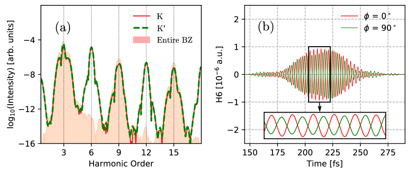
Figure 4.6: (a) High-harmonic spectrum corresponding to a linearly polarised field with amplitude of 1.5 MV/cm and frequency of 3$\omega$. The red and green lines show the valley-resolved HHG-spectrum. (b) Sixth harmonic (H6) generated by the 3$\omega$ pulse after the bicircular field broke the inversion symmetry in graphene.

While the light configuration we use is similar to that used in Ref. (Jiménez-Galán et al., 2020) for finite band-gap materials, the physical mechanism of valley-selective excitation in a zero band-gap centerosymmetric material is quite different. In gapped materials, valley-polarisation is achieved by selectively reducing the effective band gap in one of the valleys (Jiménez-Galán et al., 2020). Here, valley-polarisation is achieved only when the light-driven electrons explore the anisotropic region in the Brillouin zone.

4.3 Summary

In summary, valley polarisation in both electronic excitation and harmonic generation can be achieved in pristine graphene by tailoring the Lissajous figure of the driving pulse to the symmetry of the graphene lattice. This allows one to both break the inversion symmetry between the adjacent carbon atoms and also exploit the anisotropic regions in the valleys, taking advantage of the fact that the energy landscape of the valleys are mirror images of each other. Present work opens an avenue for a new regime of valleytronics in pristine graphene and similar materials with zero band-gap and zero Berry curvature.

Chapter 5 HHG from Spin-polarised Defects

Due to the growth processes, defects are inevitable in real solids (Hayes and Stoneham, 2012). Defects in materials can appear in the form of vacancies, impurities, interstitials (all of these can be neutral as well as charged), dislocations, etc. Defect-induced microscopic modifications in material have important impacts on its macroscopic properties (Wilson, 1931). Electronic, optical, vibrational, structural and diffusion properties of solids with defects have been thoroughly reviewed over the past century (Barker Jr and Sievers, 1975; Pantelides, 1978; Queisser and Haller, 1998; Van de Walle and Neugebauer, 2004; Bockstedte et al., 2010; Alkauskas et al., 2011; Freysoldt et al., 2014). Defect engineering is used to achieve desirable characteristics for materials such as doping, which has revolutionised the field of electronics (Bardeen and Brattain, 1949). Defects can also be highly controlled, and it is possible to create isolated defects such as nitrogen-vacancy defects in diamond (Doherty et al., 2013; Maze et al., 2008) or single photon emitters in two-dimensional materials (Tran et al., 2016a).

The influence of defects in solids is not well explored in strong-field physics. In this chapter, we aim to address interesting questions such as Is it possible to observe defect-specific fingerprints in strong-field driven electron dynamics? Or does the electron-electron interaction play a different role for defects and bulk materials? Moreover, some defects are also spin polarised in nature and therefore leads to a question of the possibility to control the electron dynamics for different spin channels independently in a non-magnetic host material. In this chapter, we will discuss how HHG is a unique probe for defects in solids.

There are theoretical predictions to understand HHG from doped semiconductors, using one-dimensional model Hamiltonians (Yu et al., 2019; Huang et al., 2017; Pattanayak et al., 2020). In Ref. (Yu et al., 2019), by using TDDFT, it is predicted that there are several orders of magnitude enhancement in the efficiency of HHG in a donor-doped semiconductor. In contrast to this in Ref. (Huang et al., 2017), with a single-active electron model, it is found that the efficiency of the second plateau from the doped semiconductor is enhanced. Similar calculation within a tight-binding Anderson model indicates that disorder might lead to well-resolved peaks in HHG (Orlando et al., 2018). The conceptual idea for tomographic imaging of shallow impurities in solids, within a one-dimensional hydrogenic model, has been developed by Corkum and co-workers (Almalki et al., 2018). Even though these pioneer works have shown that defects can influence HHG, many points remain elusive. So far, only model systems in one-dimension have been considered, and no investigation of realistic defects (through geometry optimisation and relaxation of atomic forces) has been done. Beyond the structural aspect, several other essential aspects need to be investigated in order to have a better understanding of HHG in defected-solids such as the importance of electron-electron interaction (that goes beyond single-active electron and independent-particle approximations), the role of the electron’s spin, the effect of the symmetry breaking due to the defects, etc. This chapter aims to shed light on some of these crucial questions. For that, we need to go beyond one-dimensional model Hamiltonian approach.

Monolayer hexagonal boron nitride (h-BN) is an interesting material to study electronic and optical properties. h-BN is a promising candidate for light-emitting devices in far UV region due to the strong exciton emission (Bourrellier et al., 2014, 2016). Due to technological importance, several experimental and theoretical studies have been carried out for h-BN with defects (Tran et al., 2016a, b; Huang and Lee, 2012; Zobelli et al., 2007; Alem et al., 2009; Jiménez et al., 1996; Suenaga et al., 2012; Liu et al., 2014; Thomas et al., 2015; Gilbert et al., 2017; Alem et al., 2009, 2011; Wong et al., 2015; Pierret et al., 2014; Bourrellier et al., 2016; Attaccalite et al., 2011; Azevedo et al., 2009; Orellana and Chacham, 2001; Mosuang and Lowther, 2002). Different kinds of defects in h-BN can be classified as vacancy (mono-vacancies to cluster of vacancies), antisite, and impurities. In particular, defects like monovacancies of boron and nitrogen atoms in h-BN are one of the most commonly realised defects. Recently, Zettili and co-workers have shown the possibility of engineering a cluster of vacancies and characterising them using ultra-high-resolution transmission electron microscopy (Gilbert et al., 2017; Alem et al., 2009; Wong et al., 2015). Signatures of defects in h-BN are identified by analysing cathodoluminescence and photoluminescence spectra  (Pierret et al., 2014; Bourrellier et al., 2014). It is shown that the emission band around 4 eV is originating from the transitions including deep defect levels (Attaccalite et al., 2011). Ultra-bright single-photon emission from a single layer of h-BN with nitrogen vacancy is experimentally realised, which was used for large-scale nano-photonics and quantum information processing (Tran et al., 2016a, b). In Refs. (Huang and Lee, 2012; Attaccalite et al., 2011; Azevedo et al., 2009; Liu and Cheng, 2007; Orellana and Chacham, 2001), different kinds of defects in h-BN are modelled, and their role on the electronic and optical properties have been thoroughly investigated.

In this chapter, using the well-established supercell approach to model the defects in h-BN, we analyse the influence of defects in HHG. Due to the partial ionic nature of its bonds, h-BN is a wide band-gap semiconductor with an experimental band-gap of 6 eV, which also makes it interesting for generating high-order harmonics without damaging the material. Moreover, 2D material like h-BN enables us to visualise the induced electronic density and localised defect states easily. The presence of boron or nitrogen vacancy in h-BN acts as a spin-polarised defect. These factors make h-BN an ideal candidate for exploring spin-resolved HHG in defected, non-magnetic solids. Below we will discuss HHG in h-BN with and without spin-polarised monovacancies.

5.1 Numerical Methods

Here, we employ ab initio TDDFT to simulate the strong-field driven electron dynamics in defected-solid. This allows to come up with theoretical predictions relevant for real experiments on defected-solid without empirical inputs.

5.1.1 Geometry Relaxation

Geometry optimisation was performed using the DFT code Quantum ESPRESSO (Giannozzi et al., 2009, 2017). We allow for both atomic coordinate and lattice constant relaxation. Forces were optimised to be below 10^-3 eV/Å. We used an energy cutoff of 150 Ry., and a k-point grid of 10$\times$10$\times$1 $\mathbf{k}$-points. We used a vacuum region of more than 20 Å  to isolate the monolayer from its periodic copies. We obtained relaxed lattice constants of 12.60 Å , 12.57 Å  for h-BN with a single boron vacancy ($V_{B}$), and 12.48 Å  for h-BN with a single nitrogen vacancy ($V_{N}$) while the lattice constant for pristine h-BN was found to be 12.56 Å. The structure of $V_{B}$ relaxes by lowering the local threefold symmetry (Huang and Lee, 2012). The lowering of the symmetry with the boron vacancy is attributed to the Jahn-Teller distortion, which is found to be independent of the defect concentration (Huang and Lee, 2012; Liu and Cheng, 2007; Attaccalite et al., 2011).

5.1.2 TDDFT Simulations

By propagating the Kohn-Sham equations within TDDFT, the evolution of the time-dependent current is computed using the Octopus package (Andrade et al., 2015; Castro et al., 2004). The harmonic spectrum of pristine h-BN calculated within local density approximation (LDA) and generalised gradient approximation (GGA) are presented in Fig. 5.1(a). The HHG spectrum is consistent with the choice of pseudo-potential. TDDFT within GGA with exchange and correlations of Perdew-Burke-Ernzerhof (PBE) (Perdew et al., 1996) is used for all the simulations presented here. The adiabatic approximation is used for all the time-dependent simulations. We used norm-conserving pseudo-potentials. The real-space cell was sampled with a grid spacing of 0.18 Å, and we used a 6$\times$6 $\mathbf{k}$-points grid to sample the 2D Brillouin zone. The semi-periodic boundary conditions are employed. A simulation box of 74.08 Å  along the nonperiodic dimension, including 21.17 Å of absorbing regions on each side of the monolayer is used. The absorbing boundaries are treated using the complex absorbing potential method, and the cap height h is taken as h = -1 atomic units to avoid the reflection error in the spectral region of interest (De Giovannini et al., 2015). Harmonic spectrum is calculated using equations mentioned in section 2.3.2. Spin-polarised calculations are used to address the spin-polarised vacancies.

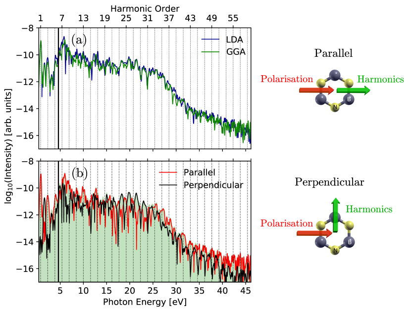
Figure 5.1: (a) High-harmonic spectrum of h-BN calculated within local density approximation (LDA), and generalised gradient approximation (GGA). (b) Harmonic spectrum in the direction parallel and perpendicular to the laser polarisation. Here, GGA is used to simulate the spectra. The two configurations are presented in the right panel. The black vertical line is the band-gap of h-BN.

The total number of excited electron is obtained by projecting the time-evolved wavefunctions ($|\psi_{n}(t)\rangle$) on the basis of the ground-state wavefunctions ($|\psi_{n^{\prime}}^{\mathrm{GS}}\rangle$)

$$N_{\mathrm{ex}}(t)=N_{e}-\frac{1}{N_{\mathbf{k}}}\sum_{n,n^{\prime}}^{\mathrm{occ.}}\sum_{\mathbf{k}}^{\mathrm{BZ}}|\langle\psi_{n,\mathbf{k}}(t)|\psi_{n^{\prime},\mathbf{k}}^{\mathrm{GS}}\rangle|^{2},$$ (5.1.1)

where $N_{e}$ is the total number of electrons in the system, and $N_{\mathbf{k}}$ is the total number of $\mathbf{k}$-points used to sample the Brillouin zone. The sum over the band indices $n$ and $n^{\prime}$ run over all occupied states.

5.1.3 Effective Band-Structure

When the energy band-structure is calculated for a supercell of the primitive unit-cell, energy-bands fold into the Brillouin zone of the supercell. An effective band-structure within the primitive unit-cell can be extracted from the eigenvalues and the eigenvectors of supercell (Ku et al., 2010; Popescu and Zunger, 2012; Medeiros et al., 2014). Let $\left|\textbf{k}n\right\rangle$ and $\left|\textbf{K}m\right\rangle$ be the eigenstates of the primitive unit-cell and supercell, respectively. A spectral weight function can be defined as

$$P_{\textbf{K}m}(\textbf{k})=\sum_{n}\left|\left\langle\textbf{K}m|\textbf{k}n\right\rangle\right|^{2}.$$ (5.1.2)

The spectral function or the effective band-structure corresponding to supercell can be expressed as a function of energy ($\mathcal{E}$) as

$$A(\textbf{k},\mathcal{E})=\sum_{m}P_{\textbf{K}m}(\textbf{k})\delta(\mathcal{E}_{m}-\mathcal{E}).$$ (5.1.3)

We have implemented a utility for unfolding band-structure in the Octopus package (Andrade et al., 2015; Castro et al., 2004; mru, ). In the present work effective single-particle band-structure or spectral function for the vacancy structures are visualised by unfolding the band-structure of 5$\times$5 supercell with 50 atoms.

5.2 Results

h-BN has a two-atoms primitive cell. We model the vacancy in a 5$\times$5 (7$\times$7) supercell with 50 atoms (98 atoms) following the method in Ref (Huang and Lee, 2012). The size of the 5$\times$5 supercell is large enough to separate the nearest defects with a distance larger than 12 Å. This avoids the interaction between the nearby defects (Huang and Lee, 2012; Liu and Cheng, 2007), and the defect wavefunctions are found to be well-localized within the supercell (Azevedo et al., 2009). In the present work, we are not considering more than one point defect. Both of our vacancy configurations (single boron as well as single nitrogen vacancy) has a total magnetic moment of +1$\mu_{B}$, consistent with the results reported in the literature  (Huang and Lee, 2012; Liu and Cheng, 2007; Azevedo et al., 2009). For the low defect concentration considered here (2% and $\sim 1\%$), the strength of the total magnetic moment is independent of the defect concentrations (Liu and Cheng, 2007). We have found that the 7$\times$7 and 5$\times$5 supercells converged to similar ground-states (Huang and Lee, 2012).

In all the present calculations, we consider a laser pulse of 15 femtosecond duration at full-width half-maximum with sine-squared envelope and a peak intensity of $13.25$ TW/cm² in the matter [for an experimental in-plane optical index $n$ of $\sim 2.65$ (Geick et al., 1966)]. The carrier wavelength of the pulse is 1600 nm, which corresponds to a photon energy of 0.77 eV. The polarisation of the laser is linear, and its direction is normal to the mirror plane of h-BN. For pristine h-BN, the band-gap is found out to be 4.73 eV within DFT-PBE level. The energy band-gap falls near the sixth harmonics of the incident photon energy, and laser parameters are well-below the damage threshold of the pristine. The symmetry of the pristine h-BN permits to observe harmonics in the parallel and perpendicular directions to the laser polarisation. The direction resolved analysis of the HHG spectrum is shown in Fig. 5.1(b). There are odd harmonics parallel to and even harmonics perpendicular to the laser polarisation. The perpendicular even harmonics are due to the anomalous current originating from the Berry curvature of the material.

5.2.1 HHG from Hexagonal Boron Nitride with a Boron Vacancy

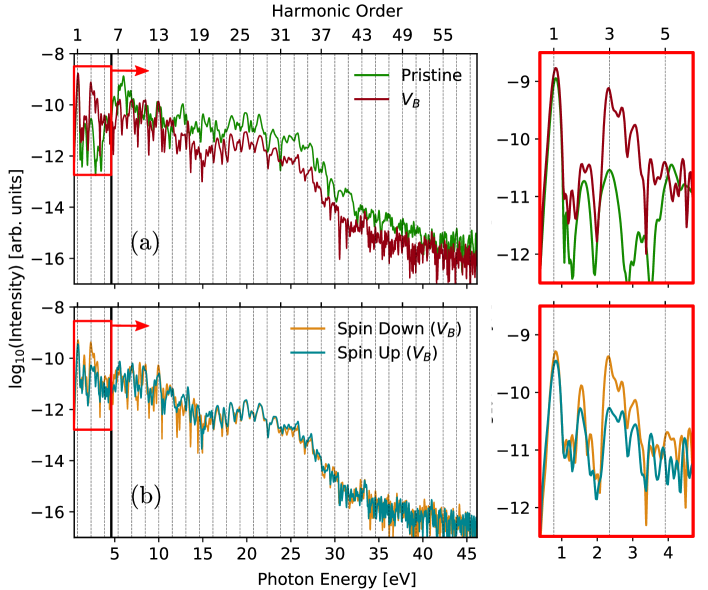
Figure 5.2: (a) High-harmonic spectrum of boron-vacant h-BN ($V_{B}$) and pristine h-BN. (b) Spin-resolved harmonic spectrum of $V_{B}$. The below band-gap portion of (a) and (b) are zoomed in the right panel. The black vertical line presents the energy band-gap of h-BN.

We start our analysis by comparing the HHG from pristine h-BN and h-BN with a boron vacancy ($V_{B}$). Removal of a boron atom makes the system spin-polarised (Huang and Lee, 2012; Liu and Cheng, 2007). The high-harmonic spectrum of $V_{B}$ and its comparison with pristine h-BN is presented in Fig. 5.2(a). The spectrum of $V_{B}$ is different from the pristine h-BN as evident from the figure. There are two distinct differences: First, the below band-gap harmonics correspond to $V_{B}$ are significantly enhanced. Second, harmonics have a much lower yield for $V_{B}$ in comparison to the pristine close to the energy cutoff.

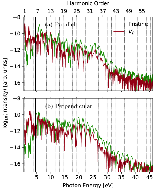
Figure 5.3: High-harmonic spectrum of boron-vacant h-BN ($V_{B}$) and pristine h-BN in the direction parallel (a) and perpendicular (b) to the laser polarisation. The black vertical line is the band-gap of h-BN.

An interesting aspect for the spin-polarised defects in a non-magnetic host is that the effect of the defect states, compared to bulk states, can be identified clearly by examining the spin-resolved spectrum. The harmonics correspond to spin-up, and spin-down channels in $V_{B}$ are shown in Fig. 5.2(b). As reflected in the figure, the below band-gap harmonics are different for both the channels. The strength of the third harmonic corresponding to the spin-down channel is much stronger (by an order of magnitude) in comparison to the associated spin-up channel. This indicates that the increase in the yield observed in Fig. 5.2(a) dominantly originates from the spin-down channel. At variance, the decrease in harmonic yield in higher energies matches well for the two spin-channels. This is a strong indication that the defects states do not play a direct role in this part of the HHG spectrum of $V_{B}$, but that bulk bands predominantly affect this spectral region, as we will discuss below. The features described in the harmonic spectrum are consistent in both parallel and perpendicular configurations as presented in Fig. 5.3.

5.2.2 Gap States and Electron Dynamics

To understand the difference in the harmonics yield associated with spin-up and spin-down channels, let us analyse the ground-state energy band-structure. The unfolded band-structures of $V_{B}$ for spin-up and spin-down channels are shown in Figs. 5.4(a), and  5.4(d), respectively. The band-structure within the band-gap region is zoomed for both the channels and shown in Figs. 5.4(b), and 5.4(c). As visible from the figure, there is one spin-up [labeled as 1 in Fig. 5.4(b)] and two spin-down [labeled as 2 and 3 in Fig. 5.4(c)] defect levels within the band-gap of pristine h-BN. One defect state corresponding to spin-up channel is pushed within the valence bands [see Fig.5.4(a)]. All three defect states within the band-gap are found to be unoccupied. These factors make the $V_{B}$ a triple acceptor. The corresponding wavefunctions for these defect states are presented in Fig. 5.4(e)-(g). The wavefunctions are found to be localized around the vacancy as expected for dispersion-less states. The $p_{x}$ and $p_{y}$ states of the nitrogen atoms in the vicinity of a boron vacancy are contributing to these defect-states, giving a $\sigma$-character to the vacancy wavefunctions (Liu and Cheng, 2007).

Figure 5.4: Spectral function for (a) spin-up and (d) spin-down components of $V_{B}$, The pristine band-structure is plotted with white dotted lines for reference. The in-gap portion of the spectral function for spin-up and spin-down components are zoomed respectively in (b) and (c), where vacancy states are recognised by 1 (for spin-up); and by 2 and 3 (for spin-down). (e)-(g) The absolute wavefunctions of the in-gap vacancy states as recognised in (b) and (c), respectively.

Unlike the pristine h-BN, spin-up and spin-down electrons in $V_{B}$ see a different band-structure near the band-gap, as the spin-resolved in-gap states are different. Therefore they evolve differently in the presence of laser pulse. It means that interband transitions and ionization involving the defects states will contribute differently to the spectrum. Hence, the spectral enhancement of the third harmonic can be understood as follows: There is an additional defect state near the valence band as visible from the spin-down band-structure, which allows spin-down electrons to be ionised or to recombine through multiple channels and contribute more to the third harmonic [see Fig. 5.2 ].

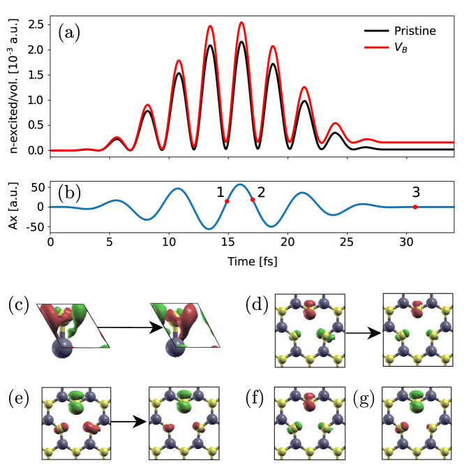
Figure 5.5: (a) Number of excited electrons per unit volume in pristine h-BN (black colour) and $V_{B}$ (red colour), and (b) vector potential of the driving laser pulse. Snap shots of the time-evolving induced electron density ($n_{ind}$) near the peak of the vector potential [marked as 1 and 2 in (b)] for (c) pristine h-BN, (d) spin-up, and (e) spin-down channels in $V_{B}$. $n_{ind}$ for (f) spin-up and (g) spin-down channels in $V_{B}$ after the end of the vector potential [marked as 3 in (b)]. Green and red colours in the induced electron density stand for positive and negative values, respectively.

It is evident from the band structure that additional defect-states effectively reduce the minimal band-gap needed to reach the conduction bands. Due to the relaxation of atoms neighbouring to the vacancy, the pristine bands get also slightly modified. However, this modification is found here to be negligible compared to the photon energy of the laser and is not further discussed. In order to understand how the presence of the defect states influence the interband tunneling, we evaluated the number of excited electrons during the laser pulse [see Fig. 5.5(a)]. In the presence of defect states, there are mostly two possible ways in which ionization can be modified compared to the bulk material. A first possibility is to have direct ionization of the defect states if they are occupied, or filling if they are originally unoccupied. Another possibility is a double sequential ionization, in which the defect states play an intermediate role in easing the ionization to the conduction bands. In $V_{B}$, there is a finite probability of finding the electrons in conduction bands even after the laser pulse is over [see the red curve in Fig. 5.5(a)]. In contrast to this, the pulse is not able to promote a significant portion of the valence electrons to the conduction bands permanently in the case of pristine h-BN as the band-gap is significantly large [see the black curve in Fig. 5.5(a)]. More precisely, for the $5\times 5$ supercell, we found that 1.6 electrons are ionised, compared to 0.25 for the case of pristine for the same cell.

To have a better understanding of possible ionization mechanisms, we also consider the induced electron density ($n_{ind}$) at two different times near the peak of the vector potential [marked as 1 and 2 in Fig. 5.5(b)] and at the end of the laser field [Fig. 5.5(f)-(g)]. As reflected in Figs. 5.5(d), and 5.5(e); the spin-polarised induced densities of $V_{B}$ have a pronounced localised component near the defects and resembles the spatial structure of the initially unoccupied defect wavefunctions [see Fig. 5.4(e)-(g)]. The induced densities at the end of the vector potential show that electrons remain in the defect states even after the laser pulse is over [see Figs. 5.5(f), and 5.5(g)]. Considering that the three defect states are originally unoccupied, we cannot conclude that more electrons are ionised to the conduction bands. It is most likely that in-gap defect states get filled during the laser excitation as  1.6 electrons are excited and $V_{B}$ is a triple acceptor.

Overall, these results show that the electron dynamics in acceptor-doped solids implies a net transfer of population to the originally unoccupied gap states, but that for a wide band-gap host no more electrons are promoted to conduction bands. This explains why only the low-order third harmonics is directly affected by the presence of spin-polarised defect states (as evidenced by the spin dependence of the spectrum). The low density of these defect states helps only fewer photons to get absorbed. We note that the irreversible population change, assisted by the defect states, ultimately implies that more energy is absorbed by the defected solid, which leads to a lower damage threshold in comparison to the pristine. However, the intensity considered here is low enough not to see such effect.

5.2.3 Effect of Electron-Electron Interaction

We found so far that the increase of the low-order harmonic yield is compatible with the presence of the defects states in the band-gap of h-BN. This is an independent-particle vision, in which we used the ground-state band-structure of $V_{B}$ to explain the observed effect on the HHG spectrum. We now turn our attention to the higher-energy harmonics, for which the harmonic yield is decreased. This seems not to be compatible with a simple vision in terms of single-particle band structure, especially with the fact that more electrons are excited by the laser pulse, as shown in Fig. 5.6(a).

To understand this, let us investigate the effect of the electron-electron interaction on the electron dynamics in $V_{B}$ and pristine h-BN. Within dipole approximation, the HHG spectrum can be expressed for the many-body system as  (Tancogne-Dejean et al., 2017b; Stefanucci and Van Leeuwen, 2013) [see Eq. (2.3.23)]

$$\textrm{HHG}(\omega)\propto\left|\mathcal{FT}\left[\int d^{3}\textbf{r}\leavevmode\nobreak\ \left\{n_{ind}(\textbf{r},t)+n_{0}(\textbf{r})\right\}\nabla v_{0}(\textbf{r})\right]+N_{e}\textbf{E}(\omega)\right|^{2}.$$ (5.2.1)

Here, $n_{ind}(\textbf{r},t)$ is the induced electron density, $v_{0}$ is the electron-nuclei interaction potential, $N_{e}$ is the total number of electrons, and E is the applied electric field. $n_{ind}(\textbf{r},t)$ is the difference of the total time-dependent electron density $n(\textbf{r},t)$ and the ground-state electron density $n_{0}(\textbf{r})$, i.e., $n_{ind}(\textbf{r},t)=n(\textbf{r},t)-n_{0}(\textbf{r})$. Also, $n(\textbf{r},t)$ is decomposed in spin-polarised fashion as $n(\textbf{r},t)$ = $n_{\uparrow}(\textbf{r},t)$ + $n_{\downarrow}(\textbf{r},t)$. If one analyses this expression, it is straightforward to understand how the introduction of vacancy can change the harmonic spectrum, through a change in the local potential structure near the defect. This results in the change in gradient of the electron-nuclei interaction potential $v_{0}$, which is independent of having electron interacting among themselves or not. Apart from this explicit source of change, it is clear that the dynamics of the induced density, evolving from a different ground-state also lead to the modifications in the harmonic spectra. The fact that the ground states are different, and hence $n_{0}(\textbf{r})$ is different, does not affect the harmonic spectrum because of the absence of time-dependence in both $n_{0}$ and $v_{0}$. The possible difference between the HHG spectra can therefore be understood in terms of independent particle effects (originating from the structural change of the nuclear potential $v_{0}$) and interaction effects through the induced density $n_{ind}$.

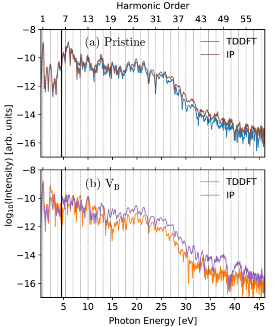
Figure 5.6: (a) High-harmonic spectrum for pristine h-BN calculated using TDDFT (blue) and the independent particle (IP) approximation (brown). (b) The harmonic spectrum for $V_{B}$ calculated using TDDFT (orange) and IP approximation (violet). The black vertical line represents the energy band-gap of pristine h-BN.

In order to disentangle these two sources of differences between pristine and defected h-BN, we simulate the harmonic spectra within an independent particle (IP) approximation by freezing the Hartree and exchange-correlation potentials to the ground-state value. The harmonic spectra for pristine h-BN and $V_{B}$ within TDDFT and IP approximation are compared in Fig. 5.6. In the case of pristine h-BN, the HHG spectra obtained by IP approximation and TDDFT are similar. Hence, there is no significant many-body effect in HHG from pristine h-BN with an in-plane laser polarisation, at least as described by PBE functional used here. A similar finding has been reported for Si (Tancogne-Dejean et al., 2017b) and MgO (Tancogne-Dejean et al., 2017a), within LDA. Only the high-order harmonics display small differences and there the electron-electron interaction reduces here the harmonic yield as found in Ref. (Yu et al., 2019). In contrast, the HHG spectra obtained by TDDFT and IP approximation are significantly different for $V_{B}$ as reflected in Fig. 5.6(b). This indicates that the electron-electron interaction is essential for HHG in defected-solids.

For the case of $V_{B}$, $n_{ind}$ is displayed in Fig. 5.5. This helps us to understand how the spatial structure of the defect states influences the harmonic spectrum. Figure 5.5(c) indicates that the spatial density oscillations are responsible for HHG in pristine h-BN. It is clear that the induced density is different in the two systems. The substantial difference in the harmonic spectra obtained by two approaches, TDDFT and IP approximation, for $V_{B}$ is due to the so-called local field effects, which is explored in detail in the following paragraphs. As we will show, it is this difference which is responsible for the decrease of the harmonic yield for $V_{B}$.

In the presence of an external electric-field, the localised induced-charge acts as an oscillating dipole near the vacancy. The dipole induces a local electric field, which screens the effect of the external electric field. This is usually referred to as local field effects. The same mechanism is responsible for the appearance of a depolarization field at the surface of a material driven by an out-of-plane electric field (Le Breton et al., 2018; Tancogne-Dejean and Rubio, 2018). It is important to stress that this induced dipole is expected to play a significant role here, due to the $\sigma$-character of the vacancy wavefunctions. The induced electric-field is directly related to the electron-electron interaction term as clearly shown in Ref. (Le Breton et al., 2018). As shown in Fig. 5.6(b), the harmonic yield at higher energies is increased if we neglect local field effects, i.e., we treat electrons at the IP approximation. Moreover, the electron-electron interaction also affects the third harmonic, as shown in Fig. 5.6(b), but lead to an increase of the harmonic yield. We, therefore, attribute this effect not to local field effects but to correlation effects. It is important to stress that in Maxwell equations, the source term of the induced electric field is the induced (summed over spin) density. Therefore, the induced electric field acts equally on the HHG from both spin channels, which is why the decrease of the yield occurs equally on both spin channels, see Fig. 5.2(b).

We conclude that the modifications in the HHG spectrum, due to a point defect, are originating from a complex interplay of two important contributions: One due to the electronic transitions including the in-gap defect states, and second arising from the electron-electron interaction. This indicates that HHG in defected-solids can not be fully addressed within IP approximation, as this can, for some cases at least, lead to a wrong qualitative prediction.

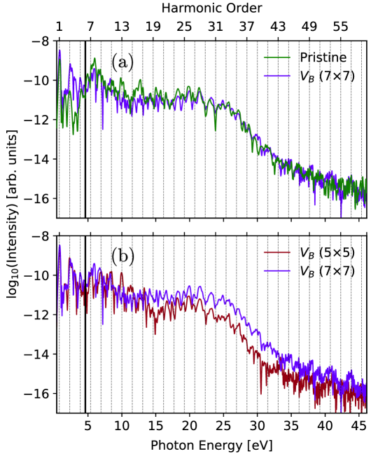
Figure 5.7: High-harmonic spectrum of $V_{B}$ in a 7$\times$7 supercell is compared with the harmonic spectrum of (a) pristine h-BN and (b) $V_{B}$ in a 5$\times$5 supercell. The black vertical line presents the energy band-gap of pristine h-BN.

Finally, we discuss the dependence of the defect concentration on the HHG spectrum by computing the HHG for a 7$\times$7 supercell with a boron vacancy, which corresponds to a $\sim$1% doping concentration. The harmonic spectrum is presented in Fig. 5.7. The third harmonic enhancement persists with comparable intensity even with a lower defect concentration [Fig. 5.7(b)], whereas the higher-energy region of the harmonic spectrum is matching well with the pristine spectrum [Fig. 5.7(a)]. This is consistent with the observation made that the higher-energy spectrum is dominated by the bulk bands. The effects due to electron-electron interaction diminishes for weaker defect concentration, while the contributions from the gap-states are consistent. This indicates that some of the effects we found here depend on the defect concentration and might not be observed below a certain concentration threshold.

5.2.4 HHG from Hexagonal Boron Nitride with a Nitrogen Vacancy

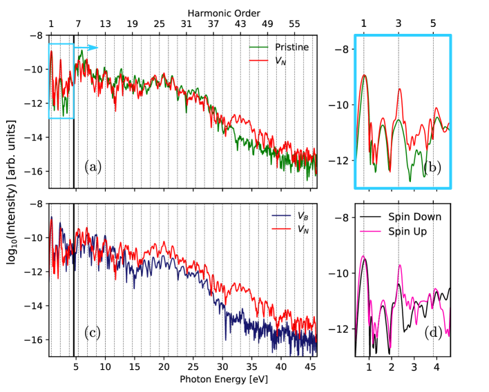
Figure 5.8: High-harmonic spectrum of (a) nitrogen vacant h-BN ($V_{N}$) and pristine h-BN, (b) $V_{N}$ and $V_{B}$, and (c) below band-gap harmonic spectrum of $V_{N}$ and pristine h-BN. (d) Spin-resolved harmonic spectrum for $V_{N}$ in the below band-gap region. The black vertical line represents the energy band-gap of pristine h-BN.

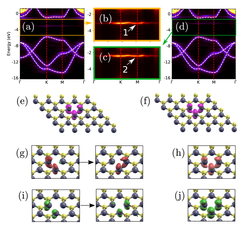
Figure 5.9: Spectral function for (a) spin-up and (d) spin-down components of $V_{N}$, The pristine band-structure is plotted with white dashed lines for reference. The in-gap portion of the spectral function for spin-up and spin-down components are zoomed respectively in (b) and (c) where in-gap vacancy states are recognised by 1 (for spin-up); and by 2 (for spin-down). (e)-(f) The absolute wavefunctions of the in-gap vacancy states 1 and 2 in (a) and (b), respectively. Snap shots of the time-evolving $n_{ind}$ near the peak of the vector potential for (g) spin-up and (i) spin-down channels; and after the end of the vector potential for (h) spin-up and (j) spin-down channels in $V_{N}$. The vector potential is shown in Fig. 5.5(b). Green and red colours in the induced electron density stand for positive and negative values, respectively.

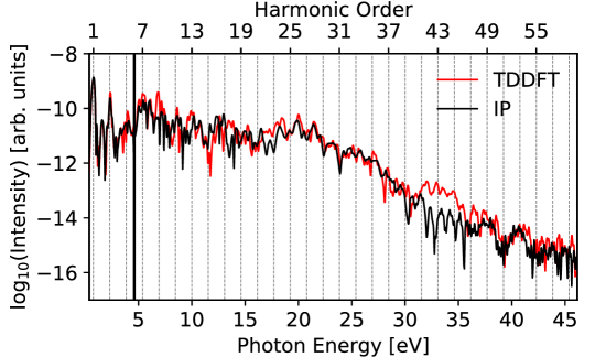
Figure 5.10: High-harmonic spectrum within TDDFT and IP approximation are compared for nitrogen-vacant h-BN ($V_{N}$). The black vertical line presents the energy band-gap of pristine h-BN.

So far, we have discussed HHG in $V_{B}$. We now explore HHG in h-BN with a nitrogen vacancy ($V_{N}$). Similar to the $V_{B}$ case, $V_{N}$ is also spin polarised. Fig. 5.8(a) presents HHG spectrum of $V_{N}$ and its comparison with the spectrum of pristine h-BN. As apparent from the figure, the spectrum of $V_{N}$ resembles more to the pristine spectrum except in the below band-gap regime, and for an increase of the yield between 30 to 35 eV. All the laser parameters are identical to the previous case of $V_{B}$. Naively, the spectra of $V_{N}$ and $V_{B}$ could be expected to look similar as one atom from the pristine h-BN has been removed in both the situations. However, this is not the case, as evident from Fig. 5.8(b) and we note that the high-energy part of the spectrum of $V_{N}$ is much closer to the one of pristine than $V_{B}$, except above 30 eV. The spectra of $V_{N}$ and $V_{B}$ are also fairly different. On close inspection of the below band-gap spectrum, one finds that the third harmonic in $V_{N}$ is significantly enhanced with respect to the pristine case [see Fig. 5.8(c)]. HHG in $V_{B}$ portrayed the identical observation. To know whether the reason behind this enhancement is identical to $V_{B}$ or not, let us analyse the spin-resolved harmonics in $V_{N}$. The below band-gap spin-resolved spectrum reveals that the third harmonic has more contribution from the spin-up electron than the spin-down electron [see Fig. 5.8(d)]. This is completely opposite to the findings in $V_{B}$ where major contribution originated from the spin-down electron. To understand this behaviour, let us explore the ground-state band-structure of $V_{N}$.

The unfolded energy band-structure of $V_{N}$ is presented in Fig. 5.9. Each of the three boron atoms has an unpaired electron after the removal of a nitrogen atom from pristine h-BN. One spin-up and one spin-down vacancy states within the band-gap are emerging and are closer to the conduction band [see Fig. 5.9(a)-(d)]. One more defect state is further pushed towards the conduction band in each case. The spin-up defect state is found to be occupied. This makes $V_{N}$ a single donor (Huang and Lee, 2012). The $p_{z}$ states of the boron atoms, which are in the vicinity of a nitrogen vacancy, contribute to the defect states. This gives a $\pi$-character to the defect wavefunctions [Fig. 5.9(e),(f)] (Huang and Lee, 2012; Azevedo et al., 2009). Similar to $V_{B}$, only gap states are analysed. The spin-up defect level is occupied and close to the conduction band, which explains the major contribution of the spin-up electron to the third harmonic in $V_{N}$. Electrons in this state can easily get ionised to the conduction bands and add more spectral weight to the third harmonic. Note that, unlike $V_{B}$, the local symmetry in $V_{N}$ is preserved, which also explains why the HHG spectrum from $V_{N}$ is close to the HHG from pristine h-BN.

The unfolded band-structures of $V_{N}$ and $V_{B}$ mainly explain the significant enhancement of the third harmonic and its different spin-polarised nature. To explain the overall difference in the harmonic spectrum, the snap shots of $n_{ind}$ in $V_{N}$ at different times along the vector potential are presented in Fig. 5.9(g)-(j). In real-space picture, defect contribution is coming from the localised induced density, which can be seen from the integral in Eq. (5.2.1). The depletion of the spin-up defect state as well as induced electron density in the spin-down defect state can be observed at the end of the pulse [see Fig. 5.9(h),(j)].

In comparison to $V_{B}$, the effect of screening due to the local field effects is weaker in the case of $V_{N}$. The weaker impact of local field effects on $V_{N}$, compared to $V_{B}$ can be attributed to the following two reasons: 1) the induced charge density has a pronounced localised component around the nitrogen vacancy. As evident from Figs. 5.9(e), and 5.9(f), the wavefunctions of spin-up and spin-down electrons have similar spatial structure, whereas the corresponding induced charge densities have opposite sign [see Fig. 5.9(g)-(j)]. This partial cancellation of the spin-resolved induced charge density makes the total induced charge to be much lower and results in a weaker local field effects. 2) For the in-plane laser polarisation, the induced dipole due to the $\pi$-like defect states get much less polarised than for the $\sigma$-like defect states. This results in weaker screening in $V_{N}$ than $V_{B}$.

The weaker local field effects in $V_{N}$ is fully consistent with the HHG spectra of $V_{N}$ within TDDFT and IP approximation as presented in Fig. 5.10. Here, the third harmonic enhancement is well captured within IP approximation, but the increase in the yield between 30 eV to 35 eV is found to originate from the electron-electron interaction. Finally, the defect states plays a role in the HHG spectrum of $V_{N}$ even at higher-orders, though these effects are feeble.

The total spectrum includes the contributions from the energy-bands of pristine h-BN as well as from transitions including gap states in $V_{B}$ and $V_{N}$ case. In both cases, we found the significant and different role of the electron-electron interaction. The harmonic spectrum of the defected solid preserves some piece of information of the pristine structure in the higher energy regime along with the characteristic signatures of the defect in the near band-gap regime, or close to the cutoff energy for $V_{N}$.

5.3 Summary

In summary, we have investigated the role of vacancy-defect in solid-state HHG. For this purpose, h-BN with a boron or a nitrogen atom vacancy is considered. In a simple minded picture, one may think that h-BN with a boron atom vacancy or with a nitrogen atom vacancy would exhibit similar HHG spectra since a single atom from h-BN has been removed. However, this is not the case as boron and nitrogen vacancies lead to qualitatively different electronic structures, and this is visible from their corresponding gap states. It has been found that by removing an atom from h-BN, either boron or nitrogen, the system becomes spin-polarised with non-zero magnetic moment near the vacancy. As a consequence, the defect-induced gap states are found to be different for each spin channel and for each vacancy, which we found to be strongly reflected in the low-order harmonics. These contributions are strongly spin-dependent, depending on the ordering and occupancy of the defect states. Altogether, we can understand the role of the defect states by analysing the spin-polarised spectra, and the findings are in accordance with the spin-polarised band-structure. This establishes one aspect of the role of defect states in strong-field dynamics in solids.

In addition, the vacancy wavefunctions of $V_{B}$ and $V_{N}$ show $\sigma$ and $\pi$-characters, respectively, which lead to different qualitative changes in the harmonic spectra of vacancies, due to the local-field effects and electron correlations. These different behaviours are stemming through the creation or not of an induced dipole, which may counteract the driving electric field, and directly depends on the spatial shape of the defect-state wavefunctions. Moreover, the electron-electron interaction also manifests itself in the decrease of the harmonic yield close to the energy cutoff in the $V_{B}$ case, whereas this effect is completely absent in the $V_{N}$ or pristine cases. This implies that the nature of the vacancies in $V_{B}$ and $V_{N}$ are entirely different, and this is reflected in their HHG spectra, even at a defect concentration as low as 2%. The HHG spectrum of $V_{N}$ is similar to the pristine h-BN, whereas the spectrum of $V_{B}$ differs significantly. These effects essentially imply that some defects are more favourable to modify the HHG spectra of the bulk materials. Thus, opening the door for tuning HHG by defect engineering in solids.

From the present work, we can also speculate what would be the effect of other known defects in h-BN. If one considers the doping impurity instead of vacancy, e.g., carbon impurity, the band-structure of h-BN remains spin-polarised in nature near the band-gap (Attaccalite et al., 2011; Huang and Lee, 2012). If a boron atom is replaced by a carbon atom, one occupied spin-up and one spin-down defect levels appear. Both the defect levels are near the conduction band with the wavefunctions contributed from the $p_{z}$ orbitals of carbon and nearby nitrogen atoms. Therefore, the carbon doping defect is expected to show qualitatively similar behaviour in the HHG spectrum as we have seen in the case of $V_{N}$. On the other hand, two defect states with occupied spin-up and unoccupied spin-down states appear near the conduction bands in the case when nitrogen is replaced with a carbon atom. The wavefunction in this case is contributed mostly from the $p_{z}$ orbitals of the carbon as well as nearby boron atoms. In this case, the enhancement in the below band-gap harmonics is expected due to the defects states near the valence bands similar to $V_{B}$. However, the effect of screening is expected to be lower compared to $V_{B}$ as the nature of wavefunctions here is similar to that of $V_{N}$.

In the case of bi-vacancy in h-BN, there are occupied defect state near the valence band and two unoccupied defect-states near the conduction band as presented in Ref. (Attaccalite et al., 2011). In this situation, if the separation between defect-states and nearby bands is small compared to the photon energy, then no significant changes in the below band-gap harmonics are expected.

Let us finally comment on the possibility of performing imaging of polarised defects in solids using HHG. As spin channels are not equivalent in the studied defects, one might think about using circularly polarised pulses to probe each spin channels independently. However, in the limit of dilute magnetic impurities, as studied here, a crystal will host as many defects with positive magnetic moments and negative ones, and the signal for up or down spin channel will appear after macroscopic average as identical.

Chapter 6 Conclusions and Future Directions

In this thesis, we have presented how HHG can be used as a method of choice to understand static and dynamical electronic properties in 2D materials. Also, we have proposed how ultrafast laser can be used for novel applications in fundamental science and technology. We have considered 2D materials with hexagonal symmetry in this thesis, and laser polarisation is deemed in-plane.

The non-perturbative electron dynamics in the presence of an intense laser field is modelled by solving TDSE with reliable approximations. Semiconductor Bloch Equation is used to solve TDSE within a single-active electron approximation. We have also solved many-electron TDSE incorporating electron-electron interaction within the framework of TDDFT.

In Chapter 5, we have demonstrated electron-electron interaction is less critical for pristine h-BN when the laser polarisation is in-plane. Moreover, a recent work offered the same conclusion for graphene, a semimetal (Li et al., 2021). This adds reliability to the single-active electron approximation, which is also widely employed for HHG from atoms. It is important to note that TDDFT calculations are computationally expensive. To get an idea about computational cost, TDDFT calculation for h-BN requires approximately 7000 core hours, whereas the same for a two-band model of gapped-graphene takes less than a core hour. Nevertheless, it is essential to list out the cases in which electron-electron interaction is critical. One such situation we reported in this thesis is the electron-dynamics in a defective material.

The electron dynamics in semimetals such as monolayer and bilayer graphene shows qualitatively similar behaviour compared to gapped-graphene, as discussed in Chapter 3. A signature of interlayer coupling in HHG from bilayer graphene is established. HHG spectrum of monolayer graphene is comparable to that of AA-stacked bilayer graphene, whereas it is significantly different for AB-stacked bilayer graphene. This signifies that the high-harmonic spectrum depends on the electronic band structure and the interband coupling between different energy-bands. We confirm that one of the signatures of electron-dynamics in a semimetal is the anomalous driver-ellipticity dependence.

The high-harmonic spectrum of gapped graphene can be easily distinguished from gapless graphene, with the presence of even harmonics. This is a consequence of the broken inversion symmetry in gapped graphene. Here, the contribution of the Berry-connection term is essential, especially close to the band-gap region. When the laser is polarised along the $\Gamma$-$\mathbf{K}$ direction, even harmonics are generated perpendicular to the laser polarisation, due to non-zero Berry curvature. On the other hand, when the laser is polarised along the $\Gamma$-$\mathbf{M}$ direction, even harmonics are parallel to the laser polarisation. The selection rules for even harmonics can be understood using simple symmetry considerations. Moreover, as the band-gap increases, the number of excited electrons in the conduction band decrease due to the inverse relation of interband transition and band-gap.

Understanding the electron dynamics enabled us to propose new methods for technological applications in Chapter 4. Hexagonal 2D materials have conduction band minima in two inequivalent points in the reciprocal space, termed $\mathbf{K}$ and $\mathbf{K}^{\prime}$ valleys. In gapped-graphene materials, valley-selective excitations can be achieved by circularly polarised light, resonant with the band-gap. This property is the basis of valleytronics. Due to vanishing band-gap and Berry curvature, resonant excitation by chiral light is not applicable to pristine graphene. We proposed a light-induced approach of valleytronics in pristine graphene, using a tailored field. In ultrafast optics, tailored field is used to obtain the desired control over electron dynamics in solids (Heinrich et al., 2021).

We have used a combination of counter-rotating circularly polarised fields with frequencies $\omega$ and 2$\omega$ to achieve valley-polarisation in pristine graphene. The resultant total field has a trefoil structure, which breaks the inversion symmetry of graphene. The energy bands near adjacent $\mathbf{K}$-points are related by mirror inversion. Therefore, the driving field leads to different electron dynamics in different $\mathbf{K}$-points, resulting in valley-selective excitation and HHG. The valley-polarisation can be controlled by changing the sub-cycle phase delay between the two pulses as the trefoil is rotated. We observed considerable valley-polarisation for strong and long-wavelength laser fields as electron traverse the anisotropic regime of the Brillouin zone. Moreover, a third harmonic probe pulse is used to measure the valley-polarisation. Here, even harmonics of the probe pulse is a measure of broken inversion symmetry, whereas which valley is polarised is embedded in the phase of these even harmonics.

Due to semimetallic nature of graphene, there is a strong interplay of interband and intraband contributions to the total harmonic spectrum. Interestingly, relative contributions of interband and intraband terms in graphene strongly depend on the polarisation of driving laser. As we have seen in Chapter 3, the characteristic driver-ellipticity dependence in HHG originates from the interband contribution. On the other hand, the dominating contribution is intraband for a bicircular driving field, as shown in Chapter 4. Therefore, it is interesting to explore the driver-polarisation dependence on the underlying mechanism for different tailor fields. Furthermore, electron dynamics and dynamical symmetries in 2D materials can be investigated using tailored fields in future.

So far, we have considered different aspects of electron dynamics in pristine materials. In Chapter 5, we analysed the effect of spin-polarised defects on HHG. This study is of fundamental importance in experiments. In particular, we have investigated the impact of vacancy defects in monolayer hBN. The HHG spectrum exhibits signatures of the defect as well as preserves most of the bulk properties of pristine h-BN. As shown in Chapter 2, using a periodic model potential, the harmonic spectrum and band structure are related. For real materials, correlating HHG directly with band structure is challenging. However, any change in the effective band structure should be imprinted in the harmonic spectrum. One such instance is mono-vacancy defect (boron or nitrogen vacancy) in h-BN. As a result of vacancy defect in h-BN, there are spin-polarised defect states within the band-gap. These defect states result in the enhancement of the below band-gap harmonics, which are also spin-polarised in nature.

We have shown that electron-electron interaction in essential to describe electron dynamics in h-BN with vacancy defect. Interband transitions to (or from) defect states result in the induced charge near vacancy. Local-field effects stemming from this induced charge is the reason for the importance of the electron-electron interaction. This effect also depends on the shape of the defect wavefunctions and defect concentration.

Our work opens interesting perspectives for further studies on strong-field electron dynamics in 2D and extended systems, especially involving isolated defects. Further works should address the possibility to monitor the electron-impurity scattering using HHG, more complex defects such as bi-vacancies, and a practical scheme for imaging buried defects in solids.

List of Publications

A. Part of this thesis

1. M. S. Mrudul, and Gopal Dixit, “High-harmonic generation from monolayer and bilayer graphene”, Physical Review B 103, 094308 (2021).

2. M. S. Mrudul, Alvaro Jimenez-Galan, Misha Ivanov, and Gopal Dixit, “Light-induced valleytronics in pristine graphene” Optica 8, 422 (2021).

3. M. S. Mrudul, Nicolas Tancogne-Dejean, Angel Rubio, and Gopal Dixit, “High- harmonic generation from spin-polarised defects in solids”, npj Computational Materials 6, 1 (2020).

4. M. S. Mrudul, Adhip Pattanayak, Misha Ivanov, and Gopal Dixit, “Direct numerical observation of real-space recollision in high-order harmonic generation from solids” Physical Review A 100, 043420 (2019).

5. M. S. Mrudul, and Gopal Dixit, “A detailed understanding of high-order harmonic generation from gapped-graphene materials” (under preparation).

B. Not part of this thesis

1. Adhip Pattanayak, M. S. Mrudul, and Gopal Dixit. “Influence of vacancy defects in solid high- order harmonic generation” Physical Review A 101, 013404 (2020).

2. Irfana N. Ansari, M. S. Mrudul, Marcelo F. Ciappina, Maciej Lewenstein, and Gopal Dixit. “ Simultaneous control of harmonic yield and energy cutoff of high-order harmonic generation using seeded plasmonically enhanced fields” Physical Review A 98, 063406 (2018).

Conferences Attended

A. International

1. PALM International School, Paris, France (28 May - 01 June, 2018).

2. ATTO2019, Szeged, Hungary (01 - 05 July, 2019).

3. QUTIF International Conference, online (22 - 25 February 2021).

4. CLEO/Europe-EQEC 2021, online (21 - 25 June 2021).

B. National

1. UFS 2017, University of Hyderabad (02 - 04 November, 2017).

2. 13${}^{\textrm{th}}$ AISAMP, IITB & TIFR, Mumbai (03 - 08 December 2018).

3. Symphy 2019, IITB (16 - 17 March 2019).

4. 22${}^{\textrm{nd}}$ NCAMP, IIT Kanpur (25 - 28 March 2019).

5. UFS 2019, IITB (07 - 09 November, 2019).

References

- (1) oct-unfold uility. https://gitlab.com/octopus-code/octopus/blob/develop/src/utils/unfold.F90.
- Agostini et al. (1979) P. Agostini, F. Fabre, G. Mainfray, G. Petite, and N. K. Rahman. Free-free transitions following six-photon ionization of xenon atoms. Physical Review Letters, 42(17):1127, 1979.
- Al-Naib et al. (2014) I. Al-Naib, J. E. Sipe, and M. M. Dignam. High harmonic generation in undoped graphene: Interplay of inter-and intraband dynamics. Physical Review B, 90(24):245423, 2014.
- Alem et al. (2009) N. Alem, R. Erni, C. Kisielowski, M. D. Rossell, W. Gannett, and A. Zettl. Atomically thin hexagonal boron nitride probed by ultrahigh-resolution transmission electron microscopy. Physical Review B, 80(15):155425, 2009.
- Alem et al. (2011) N. Alem, O. V. Yazyev, C. Kisielowski, P. Denes, U. Dahmen, P. Hartel, M. Haider, M. Bischoff, B. Jiang, S. G. Louie, et al. Probing the out-of-plane distortion of single point defects in atomically thin hexagonal boron nitride at the picometer scale. Physical Review Letters, 106(12):126102, 2011.
- Alkauskas et al. (2011) A. Alkauskas, P. Deák, J. Neugebauer, A. Pasquarello, and C. G. Van de Walle. Advanced Calculations for Defects in Materials: Electronic Structure Methods. John Wiley & Sons, 2011.
- Almalki et al. (2018) S. Almalki, A. M. Parks, G. Bart, P. B. Corkum, T. Brabec, and C. R. McDonald. High harmonic generation tomography of impurities in solids: Conceptual analysis. Physical Review B, 98(14):144307, 2018.
- Andrade et al. (2015) X. Andrade, D. Strubbe, U. De Giovannini, A. H. Larsen, M. J. T. Oliveira, J. Alberdi-Rodriguez, A. Varas, I. Theophilou, N. Helbig, M. J. Verstraete, et al. Real-space grids and the octopus code as tools for the development of new simulation approaches for electronic systems. Physical Chemistry Chemical Physics, 17(47):31371–31396, 2015.
- Ansari et al. (2021) I. N. Ansari, C. Hofmann, L. Medišauskas, M. Lewenstein, M. F. Ciappina, and G. Dixit. Controlling polarization of attosecond pulses with plasmonic-enhanced bichromatic counter-rotating circularly polarized fields. Physical Review A, 103(1):013104, 2021.
- Attaccalite et al. (2011) C. Attaccalite, M. Bockstedte, A. Marini, A. Rubio, and L. Wirtz. Coupling of excitons and defect states in boron-nitride nanostructures. Physical Review B, 83(14):144115, 2011.
- Avetissian and Mkrtchian (2016) H. Avetissian and G. Mkrtchian. Coherent nonlinear optical response of graphene in the quantum hall regime. Physical Review B, 94(4):045419, 2016.
- Avetissian and Mkrtchian (2018) H. K. Avetissian and G. F. Mkrtchian. Impact of electron-electron coulomb interaction on the high harmonic generation process in graphene. Physical Review B, 97(11):115454, 2018.
- Avetissian et al. (2013) H. K. Avetissian, G. F. Mkrtchian, K. G. Batrakov, S. A. Maksimenko, and A. Hoffmann. Multiphoton resonant excitations and high-harmonic generation in bilayer graphene. Physical Review B, 88(16):165411, 2013.
- Azevedo et al. (2009) S. Azevedo, J. R. Kaschny, C. M. C. De Castilho, and F. de Brito Mota. Electronic structure of defects in a boron nitride monolayer. The European Physical Journal B, 67(4):507–512, 2009.
- Baker et al. (2006) S. Baker, J. S. Robinson, C. Haworth, H. Teng, R. Smith, C. Chirilă, M. Lein, J. Tisch, and J. P. Marangos. Probing proton dynamics in molecules on an attosecond time scale. Science, 312(5772):424–427, 2006.
- Bardeen and Brattain (1949) J. Bardeen and W. H. Brattain. Physical principles involved in transistor action. Physical Review, 75(8):1208, 1949.
- Barker Jr and Sievers (1975) A. S. Barker Jr and A. J. Sievers. Optical studies of the vibrational properties of disordered solids. Reviews of Modern Physics, 47(S2):S1, 1975.
- Bauer and Hansen (2018) D. Bauer and K. K. Hansen. High-harmonic generation in solids with and without topological edge states. Physical Review Letters, 120(17):177401, 2018.
- Bockstedte et al. (2010) M. Bockstedte, A. Marini, O. Pankratov, and A. Rubio. Many-body effects in the excitation spectrum of a defect in sic. Physical Review Letters, 105(2):026401, 2010.
- Bourrellier et al. (2014) R. Bourrellier, M. Amato, L. H. Galvao Tizei, C. Giorgetti, A. Gloter, M. I. Heggie, K. March, O. Stéphan, L. Reining, M. Kociak, et al. Nanometric resolved luminescence in h-bn flakes: excitons and stacking order. ACS Photonics, 1(9):857–862, 2014.
- Bourrellier et al. (2016) R. Bourrellier, S. Meuret, A. Tararan, O. Stéphan, M. Kociak, L. H. G. Tizei, and A. Zobelli. Bright uv single photon emission at point defects in h-bn. Nano Letters, 16(7):4317–4321, 2016.
- Boutu et al. (2008) W. Boutu, S. Haessler, H. Merdji, P. Breger, G. Waters, M. Stankiewicz, L. J. Frasinski, R. Taieb, J. Caillat, A. Maquet, P. Monchicourt, B. Carre, and P. Salieres. Coherent control of attosecond emission from aligned molecules. Nature Physics, 4(7):545, 2008.
- Boyd (2020) R. W. Boyd. Nonlinear Optics. Academic press, 2020.
- Bruner et al. (2016) B. D. Bruner, Z. Mašín, M. Negro, F. Morales, D. Brambila, M. Devetta, D. Faccialà, A. G. Harvey, M. Ivanov, Y. Mairesse, et al. Multidimensional high harmonic spectroscopy of polyatomic molecules: detecting sub-cycle laser-driven hole dynamics upon ionization in strong mid-ir laser fields. Faraday Discussions, 194:369–405, 2016.
- Castro et al. (2004) A. Castro, M. A. L. Marques, and A. Rubio. Propagators for the time-dependent kohn–sham equations. Journal of Chemical Physics, 121(8):3425–3433, 2004.
- Castro et al. (2007) E. V. Castro, K. Novoselov, S. Morozov, N. Peres, J. L. Dos Santos, J. Nilsson, F. Guinea, A. Geim, and A. C. Neto. Biased bilayer graphene: semiconductor with a gap tunable by the electric field effect. Physical Review Letters, 99(21):216802, 2007.
- Chacón et al. (2020) A. Chacón, D. Kim, W. Zhu, S. P. Kelly, A. Dauphin, E. Pisanty, A. S. Maxwell, A. Picón, M. F. Ciappina, D. E. Kim, et al. Circular dichroism in higher-order harmonic generation: Heralding topological phases and transitions in chern insulators. Physical Review B, 102(13):134115, 2020.
- Chang et al. (1997) Z. Chang, A. Rundquist, H. Wang, M. M. Murnane, and H. C. Kapteyn. Generation of coherent soft x rays at 2.7 nm using high harmonics. Physical Review Letters, 79(16):2967, 1997.
- Charlier et al. (1991) J.-C. Charlier, X. Gonze, and J.-P. Michenaud. First-principles study of the electronic properties of graphite. Physical Review B, 43(6):4579, 1991.
- Chen and Qin (2019) Z. Y. Chen and R. Qin. Circularly polarized extreme ultraviolet high harmonic generation in graphene. Optics Express, 27(3):3761–3770, 2019.
- Chizhova et al. (2017) L. A. Chizhova, F. Libisch, and J. Burgdörfer. High-harmonic generation in graphene: Interband response and the harmonic cutoff. Physical Review B, 95(8):085436, 2017.
- Cohen and Fano (1966) H. D. Cohen and U. Fano. Interference in the photo-ionization of molecules. Physical Review, 150(1):30, 1966.
- Corkum (1993) P. B. Corkum. Plasma perspective on strong field multiphoton ionization. Physical Review Letters, 71(13):1994, 1993.
- De Giovannini et al. (2015) U. De Giovannini, A. H. Larsen, and A. Rubio. Modeling electron dynamics coupled to continuum states in finite volumes with absorbing boundaries. The European Physical Journal B, 88(3):56, 2015.
- Dimitrovski et al. (2017) D. Dimitrovski, L. B. Madsen, and T. G. Pedersen. High-order harmonic generation from gapped graphene: Perturbative response and transition to nonperturbative regime. Physical Review B, 95(3):035405, 2017.
- Dixit et al. (2018) G. Dixit, Á. Jiménez-Galán, L. Medišauskas, and M. Ivanov. Control of the helicity of high-order harmonic radiation using bichromatic circularly polarized laser fields. Physical Review A, 98(5):053402, 2018.
- Doherty et al. (2013) M. W. Doherty, N. B. Manson, P. Delaney, F. Jelezko, J. Wrachtrup, and L. C. L. Hollenberg. The nitrogen-vacancy colour centre in diamond. Physics Reports, 528(1):1–45, 2013.
- Du and Bian (2017) T.-Y. Du and X.-B. Bian. Quasi-classical analysis of the dynamics of the high-order harmonic generation from solids. Optics Express, 25(1):151–158, 2017.
- Faria et al. (2020) D. Faria, C. León, L. R. F. Lima, A. Latgé, and N. Sandler. Valley polarization braiding in strained graphene. Physical Review B, 101(8):081410, 2020.
- Ferray et al. (1988) M. Ferray, A. L’Huillier, X. F. Li, L. A. Lompre, G. Mainfray, and C. Manus. Multiple-harmonic conversion of 1064 nm radiation in rare gases. Journal of Physics B, 21(3):L31, 1988.
- Fleischer et al. (2014) A. Fleischer, O. Kfir, T. Diskin, P. Sidorenko, and O. Cohen. Spin angular momentum and tunable polarization in high-harmonic generation. Nature Photonics, 8(7):543–549, 2014.
- Floss et al. (2018) I. Floss, C. Lemell, G. Wachter, V. Smejkal, S. A. Sato, X. M. Tong, K. Yabana, and J. Burgdörfer. Ab initio multiscale simulation of high-order harmonic generation in solids. Physical Review A, 97(1):011401, 2018.
- Freysoldt et al. (2014) C. Freysoldt, B. Grabowski, T. Hickel, J. Neugebauer, G. Kresse, A. Janotti, and C. G. Van de Walle. First-principles calculations for point defects in solids. Reviews of Modern Physics, 86(1):253, 2014.
- Garg et al. (2016) M. Garg, M. Zhan, T. T. Luu, H. Lakhotia, T. Klostermann, A. Guggenmos, and E. Goulielmakis. Multi-petahertz electronic metrology. Nature, 538(7625):359, 2016.
- Geick et al. (1966) R. Geick, C. H. Perry, and G. Rupprecht. Normal modes in hexagonal boron nitride. Physical Review, 146:543–547, Jun 1966.
- Geim (2009) A. K. Geim. Graphene: status and prospects. Science, 324(5934):1530–1534, 2009.
- Ghimire and Reis (2019) S. Ghimire and D. A. Reis. High-harmonic generation from solids. Nature Physics, 15(6):10–16, 2019.
- Ghimire et al. (2011a) S. Ghimire, A. D. DiChiara, E. Sistrunk, P. Agostini, L. F. DiMauro, and D. A. Reis. Observation of high-order harmonic generation in a bulk crystal. Nature Physics, 7(2):138–141, 2011a.
- Ghimire et al. (2011b) S. Ghimire, A. D. DiChiara, E. Sistrunk, U. B. Szafruga, P. Agostini, L. F. DiMauro, and D. A. Reis. Redshift in the optical absorption of zno single crystals in the presence of an intense midinfrared laser field. Physical Review Letters, 107(16):167407, 2011b.
- Ghimire et al. (2014) S. Ghimire, G. Ndabashimiye, A. D. DiChiara, E. Sistrunk, M. I. Stockman, P. Agostini, L. F. DiMauro, and D. A. Reis. Strong-field and attosecond physics in solids. Journal of Physics B, 47(20):204030, 2014.
- Giannozzi et al. (2009) P. Giannozzi, S. Baroni, N. Bonini, M. Calandra, R. Car, C. Cavazzoni, D. Ceresoli, G. L. Chiarotti, M. Cococcioni, I. Dabo, et al. Quantum espresso: a modular and open-source software project for quantum simulations of materials. Journal of Physics: Condensed Matter, 21(39):395502, 2009.
- Giannozzi et al. (2017) P. Giannozzi, O. Andreussi, T. Brumme, O. Bunau, M. B. Nardelli, M. Calandra, R. Car, C. Cavazzoni, D. Ceresoli, M. Cococcioni, et al. Advanced capabilities for materials modelling with quantum espresso. Journal of Physics: Condensed Matter, 29(46):465901, 2017.
- Gilbert et al. (2017) S. M. Gilbert, G. Dunn, A. Azizi, T. Pham, B. Shevitski, E. Dimitrov, S. Liu, S. Aloni, and A. Zettl. Fabrication of subnanometer-precision nanopores in hexagonal boron nitride. Scientific Reports, 7(1):15096, 2017.
- Golde et al. (2008) D. Golde, T. Meier, and S. W. Koch. High harmonics generated in semiconductor nanostructures by the coupled dynamics of optical inter-and intraband excitations. Physical Review B, 77(7):075330, 2008.
- Golub and Tarasenko (2014) L. Golub and S. Tarasenko. Valley polarization induced second harmonic generation in graphene. Physical Review B, 90(20):201402, 2014.
- Gorbachev et al. (2014) R. V. Gorbachev, J. C. W. Song, G. L. Yu, A. V. Kretinin, F. Withers, Y. Cao, A. Mishchenko, I. V. Grigorieva, K. S. Novoselov, L. S. Levitov, et al. Detecting topological currents in graphene superlattices. Science, 346(6208):448–451, 2014.
- Grossmann (2018) F. Grossmann. Theoretical femtosecond physics: atoms and molecules in strong laser fields. Springer, 2018.
- Grujić et al. (2014) M. M. Grujić, M. Ž. Tadić, and F. M. Peeters. Spin-valley filtering in strained graphene structures with artificially induced carrier mass and spin-orbit coupling. Physical Review Letters, 113(4):046601, 2014.
- Gunlycke and White (2011) D. Gunlycke and C. T. White. Graphene valley filter using a line defect. Physical Review Letters, 106(13):136806, 2011.
- Gupta et al. (2003) A. K. Gupta, O. E. Alon, and N. Moiseyev. Generation and control of high-order harmonics by the interaction of an infrared laser with a thin graphite layer. Physical Review B, 68(20):205101, 2003.
- Haessler et al. (2010) S. Haessler, J. Caillat, W. Boutu, C. Giovanetti-Teixeira, T. Ruchon, T. Auguste, Z. Diveki, P. Breger, A. Maquet, B. Carré, et al. Attosecond imaging of molecular electronic wavepackets. Nature Physics, 6(3):200–206, 2010.
- Hafez et al. (2018) H. A. Hafez, S. Kovalev, J. C. Deinert, Z. Mics, B. Green, N. Awari, M. Chen, S. Germanskiy, U. Lehnert, J. Teichert, et al. Extremely efficient terahertz high-harmonic generation in graphene by hot dirac fermions. Nature, 561(7724):507–511, 2018.
- Haug and Koch (2009) H. Haug and S. W. Koch. Quantum theory of the optical and electronic properties of semiconductors. World Scientific Publishing Company, 2009.
- Hawkins et al. (2015) P. G. Hawkins, M. Y. Ivanov, and V. S. Yakovlev. Effect of multiple conduction bands on high-harmonic emission from dielectrics. Physical Review A, 91(1):013405, 2015.
- Hayes and Stoneham (2012) W. Hayes and A. M. Stoneham. Defects and defect processes in nonmetallic solids. Courier Corporation, 2012.
- Heide et al. (2018) C. Heide, T. Higuchi, H. B. Weber, and P. Hommelhoff. Coherent electron trajectory control in graphene. Physical Review Letters, 121(20):207401, 2018.
- Heinrich et al. (2021) T. Heinrich, M. Taucer, O. Kfir, P. B. Corkum, A. Staudte, C. Ropers, and M. Sivis. Chiral high-harmonic generation and spectroscopy on solid surfaces using polarization-tailored strong fields. Nature Communications, 12:3723, 2021.
- Hendry et al. (2010) E. Hendry, P. J. Hale, J. Moger, A. K. Savchenko, and S. A. Mikhailov. Coherent nonlinear optical response of graphene. Physical Review Letters, 105(9):097401, 2010.
- Hentschel et al. (2001) M. Hentschel, R. Kienberger, C. Spielmann, G. A. Reider, N. Milosevic, T. Brabec, P. Corkum, U. Heinzmann, M. Drescher, and F. Krausz. Attosecond metrology. Nature, 414(6863):509–513, 2001.
- Hermann and Fleck Jr (1988) M. R. Hermann and J. Fleck Jr. Split-operator spectral method for solving the time-dependent schrödinger equation in spherical coordinates. Physical Review A, 38(12):6000, 1988.
- Higuchi et al. (2017) T. Higuchi, C. Heide, K. Ullmann, H. B. Weber, and P. Hommelhoff. Light-field-driven currents in graphene. Nature, 550(7675):224, 2017.
- Hohenberg and Kohn (1964) P. Hohenberg and W. Kohn. Inhomogeneous electron gas. Physical Review, 136(3B):B864, 1964.
- Hohenleutner et al. (2015) M. Hohenleutner, F. Langer, O. Schubert, M. Knorr, U. Huttner, S. W. Koch, M. Kira, and R. Huber. Real-time observation of interfering crystal electrons in high-harmonic generation. Nature, 523(7562):572–575, 2015.
- Houston (1940) W. Houston. Acceleration of electrons in a crystal lattice. Physical Review, 57(3):184, 1940.
- Huang and Lee (2012) B. Huang and H. Lee. Defect and impurity properties of hexagonal boron nitride: A first-principles calculation. Physical Review B, 86(24):245406, 2012.
- Huang et al. (2017) T. Huang, X. Zhu, L. Li, X. Liu, P. Lan, and P. Lu. High-order-harmonic generation of a doped semiconductor. Physical Review A, 96(4):043425, 2017.
- Hunt et al. (2013) B. Hunt, J. D. Sanchez-Yamagishi, A. F. Young, M. Yankowitz, B. J. LeRoy, K. Watanabe, T. Taniguchi, P. Moon, M. Koshino, P. Jarillo-Herrero, et al. Massive dirac fermions and hofstadter butterfly in a van der waals heterostructure. Science, 340(6139):1427–1430, 2013.
- Hwang and Sarma (2008) E. H. Hwang and S. D. Sarma. Single-particle relaxation time versus transport scattering time in a two-dimensional graphene layer. Physical Review B, 77(19):195412, 2008.
- Ikeda (2020) T. N. Ikeda. High-order nonlinear optical response of a twisted bilayer graphene. Physical Review Research, 2(3):032015, 2020.
- Ikemachi et al. (2017) T. Ikemachi, Y. Shinohara, T. Sato, J. Yumoto, M. Kuwata-Gonokami, and K. L. Ishikawa. Trajectory analysis of high-order-harmonic generation from periodic crystals. Physical Review A, 95(4):043416, 2017.
- Jiang et al. (2018) S. Jiang, J. Chen, H. Wei, C. Yu, R. Lu, and C. Lin. Role of the transition dipole amplitude and phase on the generation of odd and even high-order harmonics in crystals. Physical Review Letters, 120(25):253201, 2018.
- Jiménez et al. (1996) I. Jiménez, A. Jankowski, L. J. Terminello, J. A. Carlisle, D. G. J. Sutherland, G. L. Doll, J. V. Mantese, W. M. Tong, D. K. Shuh, and F. J. Himpsel. Near-edge x-ray absorption fine structure study of bonding modifications in bn thin films by ion implantation. Applied Physics Letters, 68(20):2816–2818, 1996.
- Jiménez-Galán et al. (2020) Á. Jiménez-Galán, R. Silva, O. Smirnova, and M. Ivanov. Lightwave control of topological properties in 2d materials for sub-cycle and non-resonant valley manipulation. Nature Photonics, 14(12):728–732, 2020.
- Jiménez-Galán et al. (2021) Á. Jiménez-Galán, R. E. Silva, O. Smirnova, and M. Ivanov. Sub-cycle valleytronics: control of valley polarization using few-cycle linearly polarized pulses. Optica, 8(3):277–280, 2021.
- Jones et al. (2013) A. M. Jones, H. Yu, N. J. Ghimire, S. Wu, G. Aivazian, J. S. Ross, B. Zhao, J. Yan, D. G. Mandrus, D. Xiao, et al. Optical generation of excitonic valley coherence in monolayer wse 2. Nature Nanotechnology, 8(9):634–638, 2013.
- Kanai et al. (2005) T. Kanai, S. Minemoto, and H. Sakai. Quantum interference during high-order harmonic generation from aligned molecules. Nature, 435(7041):470–474, 2005.
- Kelardeh (2021) H. K. Kelardeh. Ultrafast and strong-field physics in graphene-like crystals: Bloch band topology and high-harmonic generation. arXiv preprint arXiv:2101.03635, 2021.
- Kelardeh et al. (2015) H. K. Kelardeh, V. Apalkov, and M. I. Stockman. Graphene in ultrafast and superstrong laser fields. Physical Review B, 91(4):045439, 2015.
- Kelardeh et al. (2016) H. K. Kelardeh, V. Apalkov, and M. I. Stockman. Attosecond strong-field interferometry in graphene: Chirality, singularity, and berry phase. Physical Review B, 93(15):155434, 2016.
- Kohn and Sham (1965) W. Kohn and L. J. Sham. Self-consistent equations including exchange and correlation effects. Physical Review, 140(4A):A1133, 1965.
- Korbman et al. (2013) M. Korbman, S. Y. Kruchinin, and V. S. Yakovlev. Quantum beats in the polarization response of a dielectric to intense few-cycle laser pulses. New Journal of Physics, 15(1):013006, 2013.
- Krieger and Iafrate (1986) J. B. Krieger and G. J. Iafrate. Time evolution of bloch electrons in a homogeneous electric field. Physical Review B, 33(8):5494, 1986.
- Kruchinin et al. (2018) S. Y. Kruchinin, F. Krausz, and V. S. Yakovlev. Colloquium: Strong-field phenomena in periodic systems. Reviews of Modern Physics, 90(2):021002, 2018.
- Ku et al. (2010) W. Ku, T. Berlijn, and C. C. Lee. Unfolding first-principles band structures. Physical Review Letters, 104(21):216401, 2010.
- Kumar et al. (2013) N. Kumar, J. Kumar, C. Gerstenkorn, R. Wang, H. Y. Chiu, A. L. Smirl, and H. Zhao. Third harmonic generation in graphene and few-layer graphite films. Physical Review B, 87(12):121406, 2013.
- Lakhotia et al. (2020) H. Lakhotia, H. Y. Kim, M. Zhan, S. Hu, S. Meng, and E. Goulielmakis. Laser picoscopy of valence electrons in solids. Nature, 583(7814):55–59, 2020.
- Langer et al. (2016) F. Langer, M. Hohenleutner, C. P. Schmid, C. Pöllmann, P. Nagler, T. Korn, C. Schüller, M. S. Sherwin, U. Huttner, J. T. Steiner, et al. Lightwave-driven quasiparticle collisions on a subcycle timescale. Nature, 533(7602):225, 2016.
- Langer et al. (2018) F. Langer, C. P. Schmid, S. Schlauderer, M. Gmitra, J. Fabian, P. Nagler, C. Schüller, T. Korn, P. G. Hawkins, J. T. Steiner, et al. Lightwave valleytronics in a monolayer of tungsten diselenide. Nature, 557(7703):76, 2018.
- Lanin et al. (2017) A. A. Lanin, E. A. Stepanov, A. B. Fedotov, and A. M. Zheltikov. Mapping the electron band structure by intraband high-harmonic generation in solids. Optica, 4(5):516–519, 2017.
- Le Breton et al. (2018) G. Le Breton, A. Rubio, and N. Tancogne-Dejean. High-harmonic generation from few-layer hexagonal boron nitride: Evolution from monolayer to bulk response. Physical Review B, 98(16):165308, 2018.
- Lein (2007) M. Lein. Molecular imaging using recolliding electrons. Journal of Physics B: Atomic, Molecular and Optical Physics, 40(16):R135, 2007.
- Lein et al. (2002a) M. Lein, N. Hay, R. Velotta, J. Marangos, and P. Knight. Interference effects in high-order harmonic generation with molecules. Physical Review A, 66(2):023805, 2002a.
- Lein et al. (2002b) M. Lein, N. Hay, R. Velotta, J. P. Marangos, and P. Knight. Role of the intramolecular phase in high-harmonic generation. Physical Review Letters, 88(18):183903, 2002b.
- Lewenstein et al. (1994) M. Lewenstein, P. Balcou, M. Y. Ivanov, A. L’Huillier, and P. B. Corkum. Theory of high-harmonic generation by low-frequency laser fields. Physical Review A, 49(3):2117, 1994.
- L’Huillier and Balcou (1993) A. L’Huillier and P. Balcou. High-order harmonic generation in rare gases with a 1-ps 1053-nm laser. Physical Review Letters, 70(6):774, 1993.
- Li et al. (2021) Q. Li, P. Elliott, J. K. Dewhurst, S. Sharma, and S. Shallcross. Ab initio study of ultrafast charge dynamics in graphene. Physical Review B, 103(8):L081102, 2021.
- Li et al. (2008) X. Li, X. Wang, L. Zhang, S. Lee, and H. Dai. Chemically derived, ultrasmooth graphene nanoribbon semiconductors. Science, 319(5867):1229–1232, 2008.
- Liu et al. (2018) C. Liu, Y. Zheng, Z. Zeng, and R. Li. Driving-laser ellipticity dependence of high-order harmonic generation in graphene. Physical Review A, 97(6):063412, 2018.
- Liu et al. (2017a) H. Liu, Y. Li, Y. S. You, S. Ghimire, T. F. Heinz, and D. A. Reis. High-harmonic generation from an atomically thin semiconductor. Nature Physics, 13(3):262, 2017a.
- Liu et al. (2014) P. Liu, J. Guo, L. Liu, W. Windl, G. Gu, and G. Duscher. Direct observation of defects in hexagonal boron nitride monolayers. Microscopy and Microanalysis, 20(S3):1738–1739, 2014.
- Liu and Cheng (2007) R.-F. Liu and C. Cheng. Ab initio studies of possible magnetism in a bn sheet by nonmagnetic impurities and vacancies. Physical Review B, 76(1):014405, 2007.
- Liu et al. (2017b) X. Liu, X. Zhu, P. Lan, X. Zhang, D. Wang, Q. Zhang, and P. Lu. Time-dependent population imaging for high-order-harmonic generation in solids. Physical Review A, 95(6):063419, 2017b.
- Liu et al. (2017c) X. Liu, X. Zhu, X. Zhang, D. Wang, P. Lan, and P. Lu. Wavelength scaling of the cutoff energy in the solid high harmonic generation. Optics Express, 25(23):29216–29224, 2017c.
- Luu et al. (2015) T. T. Luu, M. Garg, S. Y. Kruchinin, A. Moulet, M. T. Hassan, and E. Goulielmakis. Extreme ultraviolet high-harmonic spectroscopy of solids. Nature, 521(7553):498, 2015.
- Maiman et al. (1960) T. H. Maiman et al. Stimulated optical radiation in ruby. 1960.
- Mak et al. (2012) K. F. Mak, K. He, J. Shan, and T. F. Heinz. Control of valley polarization in monolayer mos2 by optical helicity. Nature Nanotechnology, 7(8):494–498, 2012.
- Maze et al. (2008) J. R. Maze, P. L. Stanwix, J. S. Hodges, S. Hong, J. M. Taylor, P. Cappellaro, L. Jiang, M. V. G. Dutt, E. Togan, A. S. Zibrov, et al. Nanoscale magnetic sensing with an individual electronic spin in diamond. Nature, 455(7213):644, 2008.
- McCann and Koshino (2013) E. McCann and M. Koshino. The electronic properties of bilayer graphene. Reports on Progress in Physics, 76(5):056503, 2013.
- McDonald et al. (2015) C. R. McDonald, G. Vampa, P. B. Corkum, and T. Brabec. Interband bloch oscillation mechanism for high-harmonic generation in semiconductor crystals. Physical Review A, 92(3):033845, 2015.
- Medeiros et al. (2014) P. V. C. Medeiros, S. Stafström, and J. Björk. Effects of extrinsic and intrinsic perturbations on the electronic structure of graphene: Retaining an effective primitive cell band structure by band unfolding. Physical Review B, 89(4):041407, 2014.
- Mikhailov (2007) S. A. Mikhailov. Non-linear electromagnetic response of graphene. Europhysics Letters, 79(2):27002, 2007.
- Min et al. (2007) H. Min, B. Sahu, S. K. Banerjee, and A. MacDonald. Ab initio theory of gate induced gaps in graphene bilayers. Physical Review B, 75(15):155115, 2007.
- Moon and Koshino (2012) P. Moon and M. Koshino. Energy spectrum and quantum hall effect in twisted bilayer graphene. Physical Review B, 85(19):195458, 2012.
- Mosuang and Lowther (2002) T. E. Mosuang and J. E. Lowther. Influence of defects on the h- bn to c- bn transformation. Physical Review B, 66(1):014112, 2002.
- Motlagh et al. (2018) S. A. O. Motlagh, J. S. Wu, V. Apalkov, and M. I. Stockman. Femtosecond valley polarization and topological resonances in transition metal dichalcogenides. Physical Review B, 98(8):081406, 2018.
- Motlagh et al. (2019a) S. A. O. Motlagh, F. Nematollahi, V. Apalkov, and M. I. Stockman. Topological resonance and single-optical-cycle valley polarization in gapped graphene. Physical Review B, 100(11):115431, 2019a.
- Motlagh et al. (2019b) S. A. O. Motlagh, F. Nematollahi, A. Mitra, A. J. Zafar, V. Apalkov, and M. I. Stockman. Ultrafast optical currents in gapped graphene. Journal of Physics: Condensed Matter, 32(6):065305, 2019b.
- Motlagh et al. (2020) S. A. O. Motlagh, A. J. Zafar, A. Mitra, V. Apalkov, and M. I. Stockman. Ultrafast strong-field absorption in gapped graphene. Physical Review B, 101(16):165433, 2020.
- Mrudul et al. (2020) M. Mrudul, N. Tancogne-Dejean, A. Rubio, and G. Dixit. High-harmonic generation from spin-polarised defects in solids. npj Computational Materials, 6(1):1–9, 2020.
- Mrudul et al. (2021) M. Mrudul, Á. Jiménez-Galán, M. Ivanov, and G. Dixit. Light-induced valleytronics in pristine graphene. Optica, 8(3):422–427, 2021.
- Mrudul et al. (2019) M. S. Mrudul, A. Pattanayak, M. Ivanov, and G. Dixit. Direct numerical observation of real-space recollision in high-order harmonic generation from solids. Physical Review A, 100(4):043420, 2019.
- Ndabashimiye et al. (2016) G. Ndabashimiye, S. Ghimire, M. Wu, D. A. Browne, K. J. Schafer, M. B. Gaarde, and D. A. Reis. Solid-state harmonics beyond the atomic limit. Nature, 534(7608):520–523, 2016.
- Neto et al. (2009) A. H. C. Neto, F. Guinea, N. M. R. Peres, K. S. Novoselov, and A. K. Geim. The electronic properties of graphene. Reviews of Modern Physics, 81(1):109, 2009.
- Neufeld et al. (2019) O. Neufeld, D. Podolsky, and O. Cohen. Floquet group theory and its application to selection rules in harmonic generation. Nature Communications, 10(1):1–9, 2019.
- Novoselov et al. (2004) K. S. Novoselov, A. K. Geim, S. V. Morozov, D. Jiang, Y. Zhang, S. V. Dubonos, I. V. Grigorieva, and A. A. Firsov. Electric field effect in atomically thin carbon films. Science, 306(5696):666–669, 2004.
- Odžak and Milošević (2009) S. Odžak and D. Milošević. Interference effects in high-order harmonic generation by homonuclear diatomic molecules. Physical Review A, 79(2):023414, 2009.
- Orellana and Chacham (2001) W. Orellana and H. Chacham. Stability of native defects in hexagonal and cubic boron nitride. Physical Review B, 63(12):125205, 2001.
- Orlando et al. (2018) G. Orlando, C. M. Wang, T. S. Ho, and S. I. Chu. High-order harmonic generation in disordered semiconductors. Journal of the Optical Society of America B, 35(4):680–688, 2018.
- Pantelides (1978) S. T. Pantelides. The electronic structure of impurities and other point defects in semiconductors. Reviews of Modern Physics, 50(4):797, 1978.
- Parks et al. (2020) A. M. Parks, G. Ernotte, A. Thorpe, C. R. McDonald, P. B. Corkum, M. Taucer, and T. Brabec. Wannier quasi-classical approach to high harmonic generation in semiconductors. arXiv preprint arXiv:2006.09651, 2020.
- Pattanayak et al. (2020) A. Pattanayak, M. S. Mrudul, and G. Dixit. Influence of vacancy defects in solid high-order harmonic generation. Physical Review A, 101(1):013404, 2020.
- Paul et al. (2001) P.-M. Paul, E. S. Toma, P. Breger, G. Mullot, F. Augé, P. Balcou, H. G. Muller, and P. Agostini. Observation of a train of attosecond pulses from high harmonic generation. Science, 292(5522):1689–1692, 2001.
- Pedersen et al. (2001) T. G. Pedersen, K. Pedersen, and T. B. Kriestensen. Optical matrix elements in tight-binding calculations. Physical Review B, 63(20):201101, 2001.
- Pedersen et al. (2008a) T. G. Pedersen, C. Flindt, J. Pedersen, A.-P. Jauho, N. A. Mortensen, and K. Pedersen. Optical properties of graphene antidot lattices. Physical Review B, 77(24):245431, 2008a.
- Pedersen et al. (2008b) T. G. Pedersen, C. Flindt, J. Pedersen, N. A. Mortensen, A.-P. Jauho, and K. Pedersen. Graphene antidot lattices: designed defects and spin qubits. Physical Review Letters, 100(13):136804, 2008b.
- Perdew et al. (1996) J. P. Perdew, K. Burke, and M. Ernzerhof. Generalized gradient approximation made simple. Physical Review Letters, 77(18):3865, 1996.
- Pierret et al. (2014) A. Pierret, J. Loayza, B. Berini, A. Betz, B. Plaçais, F. Ducastelle, J. Barjon, and A. Loiseau. Excitonic recombinations in h- bn: from bulk to exfoliated layers. Physical Review B, 89(3):035414, 2014.
- Popescu and Zunger (2012) V. Popescu and A. Zunger. Extracting e versus k effective band structure from supercell calculations on alloys and impurities. Physical Review B, 85(8):085201, 2012.
- Queisser and Haller (1998) H. J. Queisser and E. E. Haller. Defects in semiconductors: some fatal, some vital. Science, 281(5379):945–950, 1998.
- Reich et al. (2002) S. Reich, J. Maultzsch, C. Thomsen, and P. Ordejon. Tight-binding description of graphene. Physical Review B, 66(3):035412, 2002.
- Reimann et al. (2018) J. Reimann, S. Schlauderer, C. P. Schmid, F. Langer, S. Baierl, K. A. Kokh, O. E. Tereshchenko, A. Kimura, C. Lange, J. Güdde, et al. Subcycle observation of lightwave-driven dirac currents in a topological surface band. Nature, 562(7727):396–400, 2018.
- Rozhkov et al. (2016) A. V. Rozhkov, A. Sboychakov, A. Rakhmanov, and F. Nori. Electronic properties of graphene-based bilayer systems. Physics Reports, 648:1–104, 2016.
- Runge and Gross (1984) E. Runge and E. K. Gross. Density-functional theory for time-dependent systems. Physical Review Letters, 52(12):997, 1984.
- Rycerz et al. (2007) A. Rycerz, J. Tworzydło, and C. W. J. Beenakker. Valley filter and valley valve in graphene. Nature Physics, 3(3):172–175, 2007.
- Sato et al. (2021) S. A. Sato, H. Hirori, Y. Sanari, Y. Kanemitsu, and A. Rubio. High-order harmonic generation in graphene: Nonlinear coupling of intraband and interband transitions. Physical Review B, 103(4):L041408, 2021.
- Schaibley et al. (2016) J. R. Schaibley, H. Yu, G. Clark, P. Rivera, J. S. Ross, K. L. Seyler, W. Yao, and X. Xu. Valleytronics in 2d materials. Nature Reviews Materials, 1(11):16055, 2016.
- Schubert et al. (2014) O. Schubert, M. Hohenleutner, F. Langer, B. Urbanek, C. Lange, U. Huttner, D. Golde, T. Meier, M. Kira, S. W. Koch, and R. Huber. Sub-cycle control of terahertz high-harmonic generation by dynamical bloch oscillations. Nature Photonics, 8(2):119, 2014.
- Settnes et al. (2016) M. Settnes, S. R. Power, M. Brandbyge, and A. P. Jauho. Graphene nanobubbles as valley filters and beam splitters. Physical Review Letters, 117(27):276801, 2016.
- Shafir et al. (2012) D. Shafir, H. Soifer, B. D. Bruner, M. Dagan, Y. Mairesse, S. Patchkovskii, M. Y. Ivanov, O. Smirnova, and N. Dudovich. Resolving the time when an electron exits a tunnelling barrier. Nature, 485(7398):343–346, 2012.
- Silva et al. (2018a) R. E. F. Silva, I. V. Blinov, A. N. Rubtsov, O. Smirnova, and M. Ivanov. High-harmonic spectroscopy of ultrafast many-body dynamics in strongly correlated systems. Nature Photonics, 12(5):266, 2018a.
- Silva et al. (2018b) R. E. F. Silva, Á. Jiménez-Galán, B. Amorim, O. Smirnova, and M. Ivanov. All optical ultrafast probe of a topological phase transition. arXiv preprint arXiv:1806.11232, 2018b.
- Silva et al. (2019) R. E. F. Silva, Á. Jiménez-Galán, B. Amorim, O. Smirnova, and M. Ivanov. Topological strong-field physics on sub-laser-cycle timescale. Nature Photonics, 13(12):849–854, 2019.
- Sivis et al. (2017) M. Sivis, M. Taucer, G. Vampa, K. Johnston, A. Staudte, A. Y. Naumov, D. M. Villeneuve, C. Ropers, and P. B. Corkum. Tailored semiconductors for high-harmonic optoelectronics. Science, 357(6348):303–306, 2017.
- Smirnova et al. (2009) O. Smirnova, Y. Mairesse, S. Patchkovskii, N. Dudovich, D. Villeneuve, P. Corkum, and M. Y. Ivanov. High harmonic interferometry of multi-electron dynamics in molecules. Nature, 460(7258):972–977, 2009.
- Stefanucci and Van Leeuwen (2013) G. Stefanucci and R. Van Leeuwen. Nonequilibrium many-body theory of quantum systems: a modern introduction. Cambridge University Press, 2013.
- Stroucken et al. (2011) T. Stroucken, J. Grönqvist, and S. Koch. Optical response and ground state of graphene. Physical Review B, 84(20):205445, 2011.
- Suenaga et al. (2012) K. Suenaga, H. Kobayashi, and M. Koshino. Core-level spectroscopy of point defects in single layer h-bn. Physical Review Letters, 108(7):075501, 2012.
- Sukiasyan et al. (2010) S. Sukiasyan, S. Patchkovskii, O. Smirnova, T. Brabec, and M. Y. Ivanov. Exchange and polarization effect in high-order harmonic imaging of molecular structures. Physical Review A, 82(4):043414, 2010.
- Tamaya et al. (2016) T. Tamaya, A. Ishikawa, T. Ogawa, and K. Tanaka. Diabatic mechanisms of higher-order harmonic generation in solid-state materials under high-intensity electric fields. Physical Review Letters, 116(1):016601, 2016.
- Tancogne-Dejean and Rubio (2018) N. Tancogne-Dejean and A. Rubio. Atomic-like high-harmonic generation from two-dimensional materials. Science Advances, 4(2):eaao5207, 2018.
- Tancogne-Dejean et al. (2017a) N. Tancogne-Dejean, O. D. Mücke, F. X. Kärtner, and A. Rubio. Ellipticity dependence of high-harmonic generation in solids originating from coupled intraband and interband dynamics. Nature Communications, 8(1):745, 2017a.
- Tancogne-Dejean et al. (2017b) N. Tancogne-Dejean, O. D. Mücke, F. X. Kärtner, and A. Rubio. Impact of the electronic band structure in high-harmonic generation spectra of solids. Physical Review Letters, 118(8):087403, 2017b.
- Tancogne-Dejean et al. (2018) N. Tancogne-Dejean, M. A. Sentef, and A. Rubio. Ultrafast modification of hubbard u in a strongly correlated material: Ab initio high-harmonic generation in nio. Physical Review Letters, 121(9):097402, 2018.
- Taucer et al. (2017) M. Taucer, T. J. Hammond, P. B. Corkum, G. Vampa, C. Couture, N. Thiré, B. E. Schmidt, F. Légaré, H. Selvi, N. Unsuree, et al. Nonperturbative harmonic generation in graphene from intense midinfrared pulsed light. Physical Review B, 96(19):195420, 2017.
- Thomas et al. (2015) S. Thomas, K. Ajith, S. Chandra, and M. Valsakumar. Temperature dependent structural properties and bending rigidity of pristine and defective hexagonal boron nitride. Journal of Physics: Condensed Matter, 27(31):315302, 2015.
- Torres et al. (2010) R. Torres, T. Siegel, L. Brugnera, I. Procino, J. G. Underwood, C. Altucci, R. Velotta, E. Springate, C. Froud, I. Turcu, et al. Revealing molecular structure and dynamics through high-order harmonic generation driven by mid-ir fields. Physical Review A, 81(5):051802, 2010.
- Trambly de Laissardière et al. (2010) G. Trambly de Laissardière, D. Mayou, and L. Magaud. Localization of dirac electrons in rotated graphene bilayers. Nano Letters, 10(3):804–808, 2010.
- Tran et al. (2016a) T. T. Tran, K. Bray, M. J. Ford, M. Toth, and I. Aharonovich. Quantum emission from hexagonal boron nitride monolayers. Nature Nanotechnology, 11(1):37, 2016a.
- Tran et al. (2016b) T. T. Tran, C. Elbadawi, D. Totonjian, C. J. Lobo, G. Grosso, H. Moon, D. R. Englund, M. J. Ford, I. Aharonovich, and M. Toth. Robust multicolor single photon emission from point defects in hexagonal boron nitride. ACS Nano, 10(8):7331–7338, 2016b.
- Vampa and Brabec (2017) G. Vampa and T. Brabec. Merge of high harmonic generation from gases and solids and its implications for attosecond science. Journal of Physics B, 50(8):083001, 2017.
- Vampa et al. (2014) G. Vampa, C. McDonald, G. Orlando, D. Klug, P. Corkum, and T. Brabec. Theoretical analysis of high-harmonic generation in solids. Physical Review Letters, 113(7):073901, 2014.
- Vampa et al. (2015a) G. Vampa, T. J. Hammond, N. Thiré, B. E. Schmidt, F. Légaré, C. R. McDonald, T. Brabec, and P. B. Corkum. Linking high harmonics from gases and solids. Nature, 522(7557):462–464, 2015a.
- Vampa et al. (2015b) G. Vampa, T. J. Hammond, N. Thiré, B. E. Schmidt, F. Légaré, C. R. McDonald, T. Brabec, D. D. Klug, and P. B. Corkum. All-optical reconstruction of crystal band structure. Physical Review Letters, 115(19):193603, 2015b.
- Van de Walle and Neugebauer (2004) C. G. Van de Walle and J. Neugebauer. First-principles calculations for defects and impurities: Applications to iii-nitrides. Journal of Applied Physics, 95(8):3851–3879, 2004.
- Vitale et al. (2018) S. A. Vitale, D. Nezich, J. O. Varghese, P. Kim, N. Gedik, P. Jarillo-Herrero, D. Xiao, and M. Rothschild. Valleytronics: opportunities, challenges, and paths forward. Small, 14(38):1801483, 2018.
- Vozzi et al. (2005) C. Vozzi, F. Calegari, E. Benedetti, J.-P. Caumes, G. Sansone, S. Stagira, M. Nisoli, R. Torres, E. Heesel, N. Kajumba, et al. Controlling two-center interference in molecular high harmonic generation. Physical Review Letters, 95(15):153902, 2005.
- Walker et al. (1994) B. Walker, B. Sheehy, L. F. DiMauro, P. Agostini, K. J. Schafer, and K. C. Kulander. Precision measurement of strong field double ionization of helium. Physical Review Letters, 73(9):1227, 1994.
- Wilson (1931) A. H. Wilson. The theory of electronic semi-conductors.-ii. Proceedings of the Royal Society of London. Series A, Containing Papers of a Mathematical and Physical Character, 134(823):277–287, 1931.
- Wong et al. (2015) D. Wong, J. Velasco Jr, L. Ju, J. Lee, S. Kahn, H. Z. Tsai, C. Germany, T. Taniguchi, K. Watanabe, A. Zettl, et al. Characterization and manipulation of individual defects in insulating hexagonal boron nitride using scanning tunnelling microscopy. Nature Nanotechnology, 10(11):949, 2015.
- Wörner et al. (2010) H. J. Wörner, J. B. Bertrand, D. V. Kartashov, P. B. Corkum, and D. M. Villeneuve. Following a chemical reaction using high-harmonic interferometry. Nature, 466(7306):604–607, 2010.
- Wu et al. (2015) M. Wu, S. Ghimire, D. A. Reis, K. J. Schafer, and M. B. Gaarde. High-harmonic generation from bloch electrons in solids. Physical Review A, 91(4):043839, 2015.
- Xiao et al. (2007) D. Xiao, W. Yao, and Q. Niu. Valley-contrasting physics in graphene: magnetic moment and topological transport. Physical Review Letters, 99(23):236809, 2007.
- Xiao et al. (2012) D. Xiao, G. B. Liu, W. Feng, X. Xu, and W. Yao. Coupled spin and valley physics in monolayers of mos 2 and other group-vi dichalcogenides. Physical Review Letters, 108(19):196802, 2012.
- Yan et al. (2012) H. Yan, X. Li, B. Chandra, G. Tulevski, Y. Wu, M. Freitag, W. Zhu, P. Avouris, and F. Xia. Tunable infrared plasmonic devices using graphene/insulator stacks. Nature nanotechnology, 7(5):330–334, 2012.
- Yankowitz et al. (2012) M. Yankowitz, J. Xue, D. Cormode, J. D. Sanchez-Yamagishi, K. Watanabe, T. Taniguchi, P. Jarillo-Herrero, P. Jacquod, and B. J. LeRoy. Emergence of superlattice dirac points in graphene on hexagonal boron nitride. Nature Physics, 8(5):382–386, 2012.
- Yoshikawa et al. (2017) N. Yoshikawa, T. Tamaya, and K. Tanaka. High-harmonic generation in graphene enhanced by elliptically polarized light excitation. Science, 356(6339):736–738, 2017.
- You et al. (2017a) Y. S. You, D. A. Reis, and S. Ghimire. Anisotropic high-harmonic generation in bulk crystals. Nature physics, 13(4):345–349, 2017a.
- You et al. (2017b) Y. S. You, Y. Yin, Y. Wu, A. Chew, X. Ren, F. Zhuang, S. Gholam-Mirzaei, M. Chini, Z. Chang, and S. Ghimire. High-harmonic generation in amorphous solids. Nature Communications, 8(1):724, 2017b.
- Yu et al. (2018) C. Yu, S. Jiang, T. Wu, G. Yuan, Z. Wang, C. Jin, and R. Lu. Two-dimensional imaging of energy bands from crystal orientation dependent higher-order harmonic spectra in h- bn. Physical Review B, 98(8):085439, 2018.
- Yu et al. (2019) C. Yu, K. K. Hansen, and L. B. Madsen. Enhanced high-order harmonic generation in donor-doped band-gap materials. Physical Review A, 99(1):013435, 2019.
- Yue and Gaarde (2020) L. Yue and M. B. Gaarde. Structure gauges and laser gauges for the semiconductor bloch equations in high-order harmonic generation in solids. Physical Review A, 101(5):053411, 2020.
- Zaks et al. (2012) B. Zaks, R. B. Liu, and M. S. Sherwin. Experimental observation of electron–hole recollisions. Nature, 483(7391):580, 2012.
- Zhou et al. (2007) S. Y. Zhou, G.-H. Gweon, A. Fedorov, d. First, PN, W. De Heer, D.-H. Lee, F. Guinea, A. C. Neto, and A. Lanzara. Substrate-induced bandgap opening in epitaxial graphene. Nature Materials, 6(10):770–775, 2007.
- Zhou et al. (2008) X. Zhou, R. Lock, W. Li, N. Wagner, M. M. Murnane, and H. C. Kapteyn. Molecular recollision interferometry in high harmonic generation. Physical Review Letters, 100(7):073902, 2008.
- Zobelli et al. (2007) A. Zobelli, C. P. Ewels, A. Gloter, and G. Seifert. Vacancy migration in hexagonal boron nitride. Physical Review B, 75(9):094104, 2007.
- Zurrón et al. (2018) Ó. Zurrón, A. Picón, and L. Plaja. Theory of high-order harmonic generation for gapless graphene. New Journal of Physics, 20(5):053033, 2018.
- Zurrón-Cifuentes et al. (2019) Ó. Zurrón-Cifuentes, R. Boyero-García, C. Hernández-García, A. Picón, and L. Plaja. Optical anisotropy of non-perturbative high-order harmonic generation in gapless graphene. Optics Express, 27(5):7776–7786, 2019.