Intersection Queries for Flat Semi-Algebraic Objects in Three Dimensions and Related Problems

Abstract

Let $\mathscr{T}$ be a set of $n$ flat (planar) semi-algebraic regions in $\mathbb{R}^{3}$ of constant complexity (e.g., triangles, disks), which we call plates. We wish to preprocess $\mathscr{T}$ into a data structure so that for a query object $\gamma$, which is also a plate, we can quickly answer various intersection queries, such as detecting whether $\gamma$ intersects any plate of $\mathscr{T}$, reporting all the plates intersected by $\gamma$, or counting them. We also consider two simpler cases of this general setting: (i) the input objects are plates and the query objects are constant-degree parametrized algebraic arcs in $\mathbb{R}^{3}$ (arcs, for short), or (ii) the input objects are arcs and the query objects are plates in $\mathbb{R}^{3}$. Besides being interesting in their own right, the data structures for these two special cases form the building blocks for handling the general case.

By combining the polynomial-partitioning technique with additional tools from real algebraic geometry, we present many different data structures for intersection queries, which also provide trade-offs between their size and query time. For example, if $\mathscr{T}$ is a set of plates and the query objects are algebraic arcs, we obtain a data structure that uses $O^{*}(n^{4/3})$ storage (where the $O^{*}(\cdot)$ notation hides subpolynomial factors) and answers an arc-intersection query in $O^{*}(n^{2/3})$ time. This result is significant since the exponents do not depend on the specific shape of the input and query objects. For a parameter $s\in[n^{4/3},n^{t_{q}}]$, where ${t_{q}}\geq 3$ is the number of real parameters needed to specify a query arc, the query time can be decreased to $O^{*}((n/s^{1/{t_{q}}})^{\tfrac{2}{3}(1-1/{t_{q}})})$ by increasing the storage to $O^{*}(s)$. Our approach can be extended to many additional intersection-searching problems in three dimensions, even when the input or query objects are not flat.

1 Introduction

The general intersection-searching problem asks to preprocess a set $\mathscr{T}$ of geometric objects in $\mathbb{R}^{d}$ into a data structure, so that one can quickly report or count all objects of $\mathscr{T}$ intersected by a query object $\gamma$, or just test whether $\gamma$ intersects any object of $\mathscr{T}$ at all. Motivated by applications in various areas such as robotics, computer aided design, computer graphics, and solid modeling, intersection searching problems have been studied since the 1980’s. The early work [27, 10] on intersection searching in computational geometry mostly focused on those instances of intersection searching which could be reduced to simplex range searching in 2D or 3D, and more recently on segment-intersection or ray-shooting queries amid triangles in $\mathbb{R}^{3}$—see the survey by Pellegrini [45]. However, very little is known about more general intersection queries in $\mathbb{R}^{3}$, at least from the theoretical perspective. For instance, how quickly can one answer arc-intersection queries amid triangles in $\mathbb{R}^{3}$, or triangle-intersection queries amid arcs in $\mathbb{R}^{3}$?

In this paper we make significant, and fairly comprehensive, progress on the design of efficient solutions to general intersection-searching problems in $\mathbb{R}^{3}$. We mainly investigate intersection-searching problems in $\mathbb{R}^{3}$ where both input and query objects are flat (planar) semi-algebraic regions of constant complexity (e.g., triangles, disks), which we refer to as plates and / or (not necessarily planar) arcs. In particular, we study the following three broad classes of intersection-searching problems:

• the input objects are plates and the query objects are arcs in $\mathbb{R}^{3}$,

• the input objects are arcs and the query objects are plates in $\mathbb{R}^{3}$, and

• both input and query objects are plates in $\mathbb{R}^{3}$.

Beyond these three classes of queries, we also study some cases when both query and input objects are non-planar.

These instances of intersection searching arise naturally in applications mentioned above, and no data structures are known for them that perform better than what one would obtain using the recent semi-algebraic range-searching techniques as described below. (As far as we know, no one has yet applied these fairly recent techniques to the problems discussed in this work.)

1.1 Related work

Intersection searching is a generalization of range searching (in which the input objects are points) and point enclosure queries (in which the query objects are points), so it is not surprising that range-searching techniques have been extensively used for intersection searching [10, 8]. More precisely, the intersection condition between an input object and a query object can be written as a first-order formula involving polynomial equalities and inequalities. Using quantifier elimination, intersection queries can be reduced to semi-algebraic range queries, by working in object space, where each input object $O$ is mapped to a point $O^{*}$ and a query object $\gamma$ is mapped to a semi-algebraic region $\widetilde{\gamma}$, such that $O^{*}\in\widetilde{\gamma}$ if and only if $\gamma$ intersects the corresponding input object $O$. Alternatively, the problem can be reduced to a point-enclosure query, by working in query space, where now each input object $O$ is mapped to a semi-algebraic region $\widetilde{O}$ and each query object $\gamma$ is mapped to a point $\gamma^{*}$, so that $\gamma^{*}\in\widetilde{O}$ if and only if $\gamma$ intersects $O$. The first approach leads to a linear-size data structure with sublinear query time, and the second approach leads to a large-size data structure with logarithmic or polylogarithmic query time; see, e.g., [8, 11, 13, 26, 22, 40, 52] where this technique has been applied to simpler instances of intersection queries. One can also combine the two approaches to obtain a query-time/storage trade-off. We refer to this approach as the range-searching based approach.

The performance of these data structures depends on the number of parameters needed to specify the input and query objects. We refer to these numbers as the parametric dimension of the input and query objects, respectively. Sometimes (quite often in the present study) the performance can be improved using a multi-level data structure, where the data structure at each level is constructed in a lower-dimensional subspace of the parametric space, using only some of the degrees of freedom that specify an object. We refer to the maximum dimension of a subspace over all levels of the data structure as the reduced parametric dimension, which is equal to the maximum number of parameters of input/query objects used in a polynomial inequality in the Boolean formula describing the intersection condition; see Appendix A for a more formal definition. The performance of such a multi-level data structure depends on the reduced parametric dimension.

Roughly speaking, if the reduced parametric dimensions of the input and query objects are ${t_{o}}$ and ${t_{q}}$, respectively, and $s$, $n\leq s\leq n^{{t_{q}}}$, is a storage parameter, then using the recently developed techniques for semi-algebraic range searching based on the polynomial-partitioning method [13, 8], one can show that a query can be answered in $O^{*}((n/s^{1/{t_{q}}})^{\rho})$, where $\rho=\tfrac{1-1/{t_{o}}}{1-1/{t_{q}}}$, time using $O^{*}(s)$ storage and expected preprocessing time. See Appendix A. (As in the abstract, the $O^{*}(\cdot)$ notation hides subpolynomial factors, e.g., of the form $O(n^{\varepsilon})$, for arbitrarily small $\varepsilon>0$, and their coefficients which depend on $\varepsilon$.) We emphasize that the new approach developed in this paper eventually leads to even better bounds (see below), but we first focus on the aforementioned preliminary bound.

For example, a segment-intersection query amid $n$ triangles in $\mathbb{R}^{3}$ can be answered in $O^{*}(n^{3/4})$ time using $O^{*}(n)$ storage, in $O(\log n)$ time using $O^{*}(n^{4})$ storage, or in $O^{*}(n/s^{1/4})$ time using $O^{*}(s)$ storage, for $n\leq s\leq n^{4}$, by combining the first two solutions [44, 45]. A similar multi-level approach yields data structures in which a segment-intersection-detection query amid $n$ planes or spheres in $\mathbb{R}^{3}$ can be answered in $O^{*}(n/s^{1/3})$ time using $O^{*}(s)$ storage, for $n\leq s\leq n^{3}$, [43, 44, 45, 50]—these data structures can be extended to answering reporting queries within the same performance bound (plus an additive term that depends linearly on the output size), however, the extension to answering counting queries does not apply to the setting of spheres.

A departure from this approach is the pedestrian approach for answering ray-shooting queries. For instance, given a simple polygon $P$ with $n$ edges, a Steiner triangulation of $P$ can be constructed so that a line segment lying inside $P$ intersects only $O(\log n)$ triangles. A query is answered by traversing the query ray through this sequence of triangles [35]. The pedestrian approach has also been applied to polygons with holes in $\mathbb{R}^{2}$ [9, 35], to a convex polyhedron in $\mathbb{R}^{3}$ [28], and to polyhedral subdivisions in $\mathbb{R}^{3}$ [9, 17]. Some of the ray-shooting data structures combine the pedestrian approach with the above range-searching tools [6, 14, 26].

Recently, Ezra and Sharir [30] proposed a new approach for answering ray-shooting queries amid triangles in $\mathbb{R}^{3}$ that combines the pedestrian approach with the polynomial-partitioning scheme of Guth [32]. Roughly speaking, unlike previous approaches, which build a data structure in the $4$-dimensional parametric space of lines, Ezra and Sharir construct a polynomial partitioning in $\mathbb{R}^{3}$ on the input triangles and reduce the problem to segment-intersection queries amid a set of planes in $\mathbb{R}^{3}$. The latter can be formulated as a $3$-dimensional simplex range-searching problem, and thus their approach leads to a data structure with $O^{*}(n^{3/2})$ storage and $O^{*}(n^{1/2})$ query time, which improves upon the earlier solution [44]. Their approach also supports segment-intersection reporting queries in $O^{*}(n^{1/2}+k)$ time, where $k$ is the output size (with the same amount of storage). But it neither supports counting queries nor can it answer intersections queries with non-straight arcs (e.g. circular arcs), or handle non-flat input objects.

1.2 Our results

We present efficient data structures for (Q1)–(Q3) instances of intersection searching that perform significantly better than the best known methods, which one can obtain using the range-searching technique mentioned above. We stress that for most settings such data structures have not been studied yet. To further illustrate the versatility of our approach, we present a data structure for segment-intersection searching amid a set of spherical caps, as an illustration to the case when input objects are not planar.

As for previously studied intersection-searching problems such as segment-segment intersection searching in $\mathbb{R}^{2}$ or segment-triangle intersection searching in $\mathbb{R}^{3}$, we aim to develop faster data structures by expressing the arc-plate intersection condition (for Q1-instances, say) as a semi-algebraic predicate in which each atomic predicate uses only few of the parameters of a plate or of an arc, thereby attaining a small reduced parametric dimension. (The total number of parameters needed to represent a plate is typically quite large because of the parameters needed to specify its boundary.) For instance, if the input (resp. query) objects are plates, then ideally we would like to reduce ${t_{o}}$ (resp. ${t_{q}}$) to $3$, the number of parameters needed to represent the plane containing the plate, and eliminate the dependence on the parameters needed to represent the boundary. Several technical challenges arise in accomplishing this goal because the arc-plate intersection predicate could be quite complex, for example, because an arc may intersect a plate several times.

One of the main technical contributions of this work is to develop a general approach that addresses this challenge by combining the polynomial-partitioning technique with a battery of tools from range searching and real algebraic geometry. The most interesting among these tools is the construction of a carefully tailored cylindrical algebraic decomposition (CAD) (see [19, 23, 48]) in a suitable parametric space. We exploit for this purpose the full power of CAD (see below). Other more efficient decomposition schemes, such as vertical decomposition, do not seem to work. These tools enable us to reduce the original intersection-searching problem to simpler ones and to eliminate the asymptotic dependence on the boundary parameters completely in many cases, thereby improving ${t_{o}}$ and ${t_{q}}$ significantly, e.g., to three for the case of plates.

Another major contribution of this paper is the description of the multi-level data structure (mentioned above) for a fairly general semi-algebraic-predicate searching that allows space/query-time trade-off, using the recent techniques for semi-algebraic range searching based on the polynomial partition method [13, 8] (see Appendix A). Although this approach is similar to the multi-level partition trees described in [10, 38], extending it to polynomial-partitioning based data structures is nontrivial and, as far as we know, it has not been described in any previous paper. We regard the careful and detailed presentation of this general machinery, as presented in Appendix A, as another major contribution of this paper, and hope (or rather convinced) that it will find additional applications to other problems.

Table 1 summarizes the main results of the paper. For simplicity, we mostly focus on answering intersection-detection queries, where we want to determine whether a query object intersects any input object of $\mathscr{T}$. Our data structures extend to answering intersection-reporting queries, where we wish to report all objects of $\mathscr{T}$ that the query object intersects. By combining our intersection-detection data structures with the parametric-search framework of Agarwal and Matoušek [12], we can also answer extremal intersection queries with one degree of freedom. For example, we can answer arc-shooting queries, an extension of well studied ray-shooting queries, amid a set of plates, where for a directed query arc $\gamma$, the goal is to find the first intersection point of $\gamma$ with the plates as we walk along $\gamma$. Most of the data structures extend to answering intersection-counting queries as well, within the same asymptotic time bound. In the table, and elsewhere in the paper, when we say that an intersection query can be answered in $O^{*}(t(n))$ time, we mean that detection, counting, and extremal queries can be answered in $O^{*}(t(n))$ time and reporting queries in $O^{*}(t(n))+O(k)$ time, where $k$ is the output size. We note that we use an enhanced version of the real RAM model of computation [47] for our algorithms, in which we assume that various operations on polynomials of fixed constant degree can be performed in $O(1)$ time.

Input	Query	Storage	Query Time Exp.		Reference
		Exp.	Old	New
Plates	Arc/Curve	$4/3$	$(1-\tfrac{1}{{t_{o}}})(1-\tfrac{1}{3({t_{q}}-1)})$	$2/3$	Theorem 2.1
Plates	Arc/Curve	$3/2$	$(1-\tfrac{1}{{t_{o}}})(1-\tfrac{1}{2({t_{q}}-1)})$	$\tfrac{2}{3}(1-\tfrac{1}{(2({t_{q}}-1)})$	Theorem 5.1
Triangles	Arc/Curve	$1$	$8/9$	$4/5$	Theorem 7.1
Triangles	Arc/Curve	$11/9$	$\tfrac{8}{9}(1-\tfrac{2}{9({t_{q}}-1)})$	$2/3$	Theorem 2.2
Segments	Plate	$3/2$	$\tfrac{3}{4}(1-\tfrac{1}{2({t_{q}}-1)})$	$1/2$	Theorem 8.6
Arcs/Curves	Plate	$3/2$	$(1-\tfrac{1}{{t_{o}}})(1-\tfrac{1}{2({t_{q}}-1)})$	$\tfrac{3}{4}(1-\tfrac{1}{t})$	Theorem 8.9
Triangles	Triangle	$3/2$	$5/8$	$1/2$ (report)	Theorem 9.1
Triangles	Triangle	$3/2$	$5/8$	$5/9$ (count)	Theorem 9.2
Plates	Plate	$3/2$	$(1-\tfrac{3}{2{t_{q}}})$	$\max\left\{\frac{2{t_{q}}-3}{3({t_{q}}-1)},\frac{3({t_{o}}-1)}{4{t_{o}}}\right\}$	Theorem 9.3
Spherical caps	Segment	$5/4$	$11/14$	$3/4$	Theorem 10.1
Spherical caps	Segment	$3/2$	$5/7$	$27/40$	Theorem 10.1

Table 1: Summary of results. For simplicity, we state the bounds for fixed storage parameters. Here ${t_{o}},{t_{q}}$ are the reduced parametric dimensions of the curves supporting the edges of the input and the query plates, respectively. Storage is $O^{*}(n^{\alpha})$ and query time is $O^{*}(n^{\beta})$ using the range searching approach in Appendix A and $O^{*}(n^{\gamma})$ using our new technique, respectively. We specify the values of $\alpha$, $\beta$, and $\gamma$ for each result. For reporting queries, the query procedure spends an additional $O(k)$ time to report the output of size $k$. For counting queries, the data structures count the number of connected components of the intersections between the input objects and the query object (which may be a set of points or a set of arcs), and not the number of input objects intersected by the query object (except when both input and query objects are triangles). We comment that for the case of triangles vs. triangles, the exponent $5/8$ in the query time is obtained by setting the parametric dimension to $4$ after some processing (without further processing the parametric dimension is $9$).

In the rest of this section, we describe the specific results we obtain, compare them with the best-known bounds or rather with best bounds achievable with known (recent) techniques, and briefly sketch the key ideas that lead to the improved bounds. But we first need a definition: We refer to a connected path $\gamma$ as a parametrized (algebraic) arc if it is the restriction of a real algebraic curve $\sigma\colon I\rightarrow\mathbb{R}^{3}$, where $I$ is either the real axis or the unit circle, to a subinterval $[a,b]\subseteq I$. The parametric dimension $t$ of $\gamma$ is the number of real parameters needed to describe $\gamma$. Two of these parameters, namely $a$, $b$, specify the respective endpoints $\sigma(a)$ and $\sigma(b)$. We assume that the degree of the polynomials defining $\sigma$ is also bounded by some constant, the dependence on which will only show up in the constants hiding in the $O^{*}(\cdot)$ notation. See Section 2 for a more detailed discussion on the parametrization of algebraic arcs.

Intersection searching with arcs amid plates.

Let $\mathscr{T}$ be a set of $n$ plates in $\mathbb{R}^{3}$ in general position, i.e., any plane contains only $O(1)$ plates of $\mathscr{T}$, and any line is contained in supporting planes of $O(1)$ plates of $\mathscr{T}$ (see Sections 2, 5, and 7). Let $\Gamma$ be a family of parametrized algebraic arcs in $\mathbb{R}^{3}$. Let ${t_{o}},{t_{q}}$ be the reduced parametric dimensions of $\mathscr{T}$ and $\Gamma$, respectively. We present several data structures for answering arc-intersection queries amid $\mathscr{T}$ with arcs in $\Gamma$. We note that the general-position assumption on the input plates is necessary, as discussed in the beginning of Section 2.

Our first main result is an $O^{*}(n^{4/3})$-size data structure that can be constructed in $O^{*}(n^{4/3})$ expected time and that supports arc-intersection queries in $O^{*}(n^{2/3})$ time (see Section 2). (In fact, the exponent in the query time is slightly less than $2/3$, as stated in Theorem 5.1.) It is surprising that the asymptotic query time bound depends neither on the parametric dimension of the query arc nor on that of the input plates, though the coefficients hiding in the $O^{*}$-notation do depend on them. If we follow the range-searching based approach outlined above (and use Theorem A.4 in Appendix A), an $O^{*}(n^{4/3})$-size data structure will answer a query in time $O^{*}(n^{\rho})$, where $\rho=(1-\tfrac{1}{{t_{o}}})(1-\tfrac{1}{3({t_{q}}-1)})$. For instance, if the input is a set of triangles and query arcs are circular arcs, then ${t_{o}}=9$ and ${t_{q}}=8$ and therefore $\rho\approx 0.847$.

As in [30], we also construct a polynomial partitioning in $\mathbb{R}^{3}$, i.e., we compute a tri-variate partitioning polynomial $F$ of degree $O(D)$, for a sufficiently large constant $D$, using the algorithm in [8]. The zero set $Z(F)$ of $F$ partitions $\mathbb{R}^{3}$ into cells, which are the connected components of $\mathbb{R}^{3}\setminus Z(F)$. For each cell $\tau$ of $\mathbb{R}^{3}\setminus Z(F)$, the plates whose relative boundaries intersect $\tau$ are called narrow at $\tau$, and the other plates intersecting $\tau$ are called wide. For each cell $\tau$, we recursively preprocess the narrow plates of $\tau$, and construct a secondary data structure for the wide plates of $\tau$. A query is answered by traversing all cells of $\mathbb{R}^{3}\setminus Z(F)$ that are intersected by the query arc. At each such cell, intersection with narrow plates is handled recursively, but the intersection with wide plates is processed using the secondary data structure. Handling wide plates is significantly more challenging than in [30] because the query object, as well the edges of the plates, are arcs instead of line segments.

We handle wide input plates using a completely different approach that not only generalizes to algebraic arcs but also simplifies, in certain aspects, the technique of [30] for segment-intersection searching, and extends to answering intersection-counting queries. Roughly speaking, we construct a carefully tailored CAD of a suitable parametric space, where the CAD is induced by the partitioning polynomial. For a plate $\Delta$ and a partitioning polynomial $F$, $\Delta\setminus Z(F)$ consists of several connected components. The CAD is used to further subdivide each component into smaller pieces (pseudo-trapezoids) and label each piece that is fully contained in the relative interior of $\Delta$. The label is an explicit semi-algebraic representation of that piece, of constant complexity, that depends only on the equation of $h_{\Delta}$, the plane supporting $\Delta$ (and not on the boundary of $\Delta$), and on the fixed polynomial $F$ (Sections 3.2 and 3.3). These labels enable us to formulate an arc-intersection query on wide plates as a three-dimensional semi-algebraic range query (Section 3.4), which is how we get the query time to be independent of the parametric dimension of the plates.

Next, we present data structures (in Sections 4 and 5) for answering arc-intersection queries amid plates, that provide a trade-off between size and query time. We first present such data structures for wide plates by using the CAD labels and the general framework of space/query-time trade-off described in Appendix A. In general, if the query arcs have reduced parametric dimension ${t_{q}}$, then, using $O^{*}(s)$ storage, $s\in[n,n^{{t_{q}}}]$, a query can be answered in $O^{*}\left((n/s^{1/{t_{q}}})^{\tfrac{2}{3(1-1/{t_{q}})}}\right)$ time. We next prove that, if the query arcs are planar, then by exploiting the geometry of planar arcs, ${t_{q}}$ can be improved to the reduced parametric dimension of the curves supporting the arcs in $\Gamma$, by effectively eliminating the dependence on the endpoints of the query arcs (see Sections 4.2 and 4.3). For example, if the query objects are circular arcs, their parametric dimension is eight (three for specifying the supporting plane, three for specifying the containing circle in that plane, and two for the endpoints). We show how to improve the query time from $O^{*}(n^{13/21})$ (the query time bound for ${t_{q}}=8$) to $O^{*}(n^{3/5})$ (the bound for ${t_{q}}=6$), with the same asymptotic storage complexity $O^{*}(n^{3/2})$, by constructing a multi-level data structure in which each level is built in at most six dimensions. We note that the query time of a data structure, with storage parameter $s$, based on range-searching approach would be $O^{*}((n/s^{1/{t_{q}}})^{\tfrac{1-1/{t_{o}}}{1-1/{t_{q}})}})$, which is larger because ${t_{o}}$ is typically much larger than $3$.

With the space/query-time trade-off for wide plates at our disposal, we are able to obtain a similar trade-off for general plates in Section 5. By combining our polynomial-partitioning scheme (described in Section 2) with multi-level data structures for semi-algebraic and point-enclosure queries, for a storage parameter $s\in[n,n^{{t_{q}}}]$, we show that an arc-intersection query can be answered in time

$$O^{*}\biggl{(}\frac{n^{2-3/{t_{o}}}}{s^{1-2/{t_{o}}}}+\biggl{(}\frac{n^{{t_{q}}}}{s}\biggr{)}^{\tfrac{2}{3({t_{q}}-1)}}\biggr{)},$$

using $O^{*}(s)$ space and preprocessing. If $\Gamma$ is a family of planar arcs, then ${t_{q}}$ in the above bound is the reduced parametric dimension of the curves supporting the arcs in $\Gamma$.

We next present in Section 6 a data structure for arc-intersection queries for the case when the query arcs lie on a fixed $2$-dimensional algebraic surface of constant degree. Such a data structure is needed as a subroutine for the main data structure described in Section 2. Again, we combine polynomial partitioning technique with CAD. Using the fact that the query arcs lie on a fixed $2$-dimensional surface, we obtain a data structure of $O^{*}(n)$ size with $O^{*}(n^{2/3})$ query time.

We conclude the first part of the paper in Section 7 by showing that if $\mathscr{T}$ is a set of triangles in $\mathbb{R}^{3}$, then the intersection condition of a triangle with a parametrized algebraic arc of constant complexity can be expressed as a semi-algebraic predicate in which each polynomial inequality uses at most five of the nine parameters that specify a triangle, namely, ${t_{o}}=5$ in this case. This is accomplished by constructing a CAD induced by a suitable polynomial in the joint space of query arcs and the space of planes in $\mathbb{R}^{3}$, i.e., in $\mathbb{R}^{t+3}$ if the parametric dimension of the curves supporting the query arcs is $t$, and building a separate data structure for each cell of the CAD. This leads to an $O^{*}(n)$-size data structure for triangles that answers arc-intersection queries in $O^{*}(n^{4/5})$ query time, a significant improvement over the best achievable query time of $O^{*}(n^{8/9})$, using the known machinery. By plugging this data structure into our machinery, for a storage parameter $s\in[n,n^{{t_{q}}}]$, we obtain a data structure of size $O^{*}(s)$ that can answer an arc-intersection query in time $O^{*}\biggl{(}n^{7/5}/s^{3/5}+(n^{{t_{q}}}/s)^{\tfrac{2}{3({t_{q}}-1)}}\biggr{)}$; if the arcs in $\Gamma$ are planar then ${t_{q}}$ is the reduced parametric dimension of the curves supporting the arcs in $\Gamma$ (with respect to triangles).

Intersection searching with plates amid arcs.

Next, we present data structures for the complementary setup where the input objects are arcs and we query with a plate (see Section 8). We first show that we can preprocess a set $L$ of $n$ lines in $\mathbb{R}^{3}$, in expected time $O^{*}(n^{3/2})$, into a data structure of size $O^{*}(n^{3/2})$ by constructing a polynomial partitioning in $\mathbb{R}^{3}$ on input lines, so that a plate-intersection query in $L$ can be answered in $O^{*}(n^{1/2})$ time. It constructs a CAD in $\mathbb{R}^{3}$ induced by the partitioning polynomial and uses a topological result to reduce the problem to plane-intersection searching amid a set of segments. The latter can be formulated as a $3$-dimensional simplex range-searching problem. The best achievable query time for a data structure of size $O^{*}(n^{3/2})$, based on range searching, is $O^{*}(n^{\rho})$, where $\rho=\tfrac{3}{4}(1-\tfrac{1}{2({t_{q}}-1)})$, where ${t_{q}}$ is the parametric dimension of the query plates. By combining our data structure with the semi-algebraic-predicate query machinery, for a parameter $s\in[n,n^{{t_{q}}}]$, we can answer an intersection query in the improved time $O^{*}(n^{5/4}/s^{1/2}+(n^{{t_{q}}}/s)^{\frac{1}{2{t_{q}}-3}})$. This data structure easily extends, with the same asymptotic performance, to the case where the input is a set of line segments rather than full lines.

Finally, we consider the case where the input consists of a set of $n$ algebraic arcs of reduced parametric dimension ${t_{o}}$ in general position, i.e., any plane contains only $O(1)$ input arcs. The query objects remain plates of reduced parametric dimension ${t_{q}}$. Since a query plate may intersect an input arc multiple times, our data structure for line segments does not extend to arcs. Instead, we follow an approach similar to that in Section 2 and combine polynomial partitioning with a CAD in a $5$-dimensional parametric space. For a storage parameter $s\in[n,n^{{t_{q}}}]$, the query time is $O^{*}\biggl{(}(n^{3}/s)^{\frac{{t_{o}}-1}{2{t_{o}}}}+(n^{{t_{q}}}/s)^{\tfrac{3({t_{o}}-1)}{2{t_{o}}(2{t_{q}}-3)}}\biggr{)}$. See Theorem 8.9. In particular, for $s=n^{3/2}$, the query time is $O^{*}(n^{\frac{3}{4}(1-1/{t_{o}})})$, which, interestingly, is asymptotically independent of ${t_{q}}$. As a comparison point, the exponent in the query time with the range-searching approach would be $(1-\tfrac{1}{{t_{o}}})(1-\tfrac{1}{2({t_{q}}-1)})$. In other words, the new approach reduces ${t_{q}}$ to $3$, eliminating the dependence on the boundary of the query plate.

Intersection searching with plates amid plates.

The above results can be used to provide simple solutions for the case where both input and query objects are plates (see Section 9). For simplicity, assume first that both input and query objects are triangles in $\mathbb{R}^{3}$. For $s\in[n,n^{4}]$, using $O^{*}(s)$ storage, a detection/reporting/extremal query can be answered in time $O^{*}(n^{5/4}/s^{1/2}+n^{4/5}/s^{1/5})$. For counting queries, the query time is $O^{*}(n^{5/4}/s^{1/2}+n^{8/9}/s^{2/9})$. (This is the only case in this paper in which arc-intersection-counting queries are more expensive than arc-intersection-detection queries.)

The technique can be extended to the case where both input and query objects are arbitrary plates. In this case, the boundary of a plate consists of $O(1)$ algebraic arcs of constant complexity. Let ${t_{o}}$ and ${t_{q}}$ be the reduced parametric dimensions of the input and the query plates, respectively. We obtain a data structure of $O^{*}(n^{3/2})$ size with query time $O^{*}(n^{\rho})$, where $\rho=\max\left\{\frac{2{t_{q}}-3}{3({t_{q}}-1)},\frac{3({t_{o}}-1)}{4{t_{o}}}\right\}$. If ${t_{o}}={t_{q}}=t\geq 3$, then $\rho=\frac{3(t-1)}{4t}$.

Our data structure for the plate-plate case also works if the input and query objects are constant-complexity, not necessarily convex three-dimensional polyhedra. This is because an intersection between two polyhedra occurs when their boundaries meet, unless one of them is fully contained in the other, and the latter situation can be easily detected. We can therefore just triangulate the boundaries of both input and query polyhedra and apply the triangle-triangle intersection-detection machinery.

The case of spherical caps.

Finally, we present, in Section 10, an application of our technique to an instance where the input objects are not flat. Specifically, we show how to answer segment-intersection queries amid spherical caps (each being the intersection of a sphere with a halfspace). For a storage parameter $s\in[n,n^{6}]$, a query can be answered in $O^{*}(n^{11/7}/s^{5/7}+n^{9/10}/s^{3/20})$ time.

2 Intersection Searching with Query Arcs amid Plates

We begin by describing the parametrization/representation of query arcs and input plates. A family $\Gamma$ of parametrized algebraic arcs in $\mathbb{R}^{3}$ is defined as follows. Recall that a function $y=f(x_{1},\ldots,x_{m})$ in $m$ variables is called an algebraic function if it solves a polynomial equation in $m+1$ variables of the form $P_{f}(y,x_{1},\ldots,x_{m})=0$. We say that $P_{f}$ defines the function $f$, and that the degree of $P_{f}$ is the degree of $f$. For some fixed constant parameter $t>0$, let $\hat{x}(u,\alpha),\hat{y}(u,\alpha),\hat{z}(u,\alpha)\colon\mathbb{R}^{t}\times\mathbb{R}\rightarrow\mathbb{R}$ be $(t+1)$-variate algebraic functions of bounded degree each. For a point $\delta\in\mathbb{R}^{t}$, let $x_{\delta}(\alpha)=\hat{x}(\delta,\alpha)$, $y_{\delta}(\alpha)=\hat{y}(\delta,\alpha)$, and $z_{\delta}(\alpha)=\hat{z}(\delta,\alpha)$ be the corresponding univariate algebraic functions obtained by fixing $\delta$. Then $\sigma_{\delta}(\alpha)\coloneqq(x_{\delta}(\alpha),y_{\delta}(\alpha),z_{\delta}(\alpha))$, $\alpha\in\mathbb{R}$, defines a parametrized algebraic curve. We note that we allow a more general parametrization than the commonly used rational parametrization (where each of $\hat{x},\hat{y},\hat{z}$ is a ratio of two polynomials) that parametrizes only zero-genus algebraic curves [51]. There is also some work on parametrizing algebraic curves (of genus at most $6$) using radicals [49]. Fast algorithms are known for computing rational and radical parametrization of algebraic curves if they exist [1, 2, 49]. We are unaware of (efficient) algorithms for computing a more general (global) uni-parametrizations of algebraic curves, though a local parametrization can be computed using Puiseux series [41] (which is not very useful in our setting) or an approximate parametrization can be computed [46]. Here we assume that a global parametrization of the above form is given for the curves supporting the query arcs. Let $\mathbb{E}_{t}\coloneqq\mathbb{R}^{t}$ denote the space of these curves. For a pair of real values $\alpha^{-},\alpha^{+}$, $\gamma(\delta,\alpha^{-},\alpha^{+})$ defines the algebraic arc $\gamma\coloneqq\{\sigma_{\delta}(\alpha)\mid\alpha^{-}\leq\alpha\leq\alpha^{+}\}$ in $\mathbb{R}^{3}$; $\gamma$ is an empty arc if $\alpha^{+}<\alpha^{-}$. Set

$$\Gamma\coloneqq\{\gamma(\delta,\alpha^{-},\alpha^{+})\mid\delta\in\mathbb{E}_{t}\;\mbox{and}\;\alpha^{-},\alpha^{+}\in\mathbb{R}\}.$$

The parametric dimension of $\Gamma$ is $t+2$. We identify the space of arcs in $\Gamma$ with $\mathbb{R}^{t+2}$, which we refer to as the query space and in which an arc $\gamma(\delta,\alpha^{-},\alpha^{+})$ is mapped to the point $(\delta,\alpha^{-},\alpha^{+})$.

Next, we describe the space of input plates. Recall that a plate is a planar semi-algebraic set of constant complexity in $\mathbb{R}^{3}$. For simplicity, without loss of generality, we assume that the Boolean formula describing the plate consists only of conjunctions, as disjunctions can be handled by decomposing each plate into $O(1)$ plates, each described by a conjunction of polynomial inequalities. Let $k,r_{1},\ldots,r_{k}>0$ be constant integers. For each $1\leq i\leq k$, let $f_{i}(u_{1},\ldots,u_{r_{i}},x,y,z)$ be an $(r_{i}+3)$-variate polynomial of constant degree. For a point $\xi=(a_{0},b_{0},c_{0})\in\mathbb{R}^{3}$, let $h_{\xi}$ be the (non-vertical) plane $z=a_{0}x+b_{0}y+c_{0}$. For given points $\delta_{1}\in\mathbb{R}^{r_{1}},\ldots,\delta_{k}\in\mathbb{R}^{r_{k}},\xi\in\mathbb{R}^{3}$, we define the plate

$$\Delta(\delta_{1},\ldots,\delta_{k},\xi)\coloneqq\left\{p\in\mathbb{R}^{3}\mid\bigwedge_{i=1}^{k}(f_{i}(\delta_{i},p)\geq 0)\wedge p\in h_{\xi}\right\}.$$

We define a family $\mathbb{T}$ of plates as

$$\mathbb{T}\coloneqq\{\Delta(\delta_{1},\ldots,\delta_{k},\xi)\mid\delta_{1}\in\mathbb{R}^{r_{1}},\ldots,\delta_{k}\in\mathbb{R}^{r_{k}},\xi\in\mathbb{R}^{3}\}.$$ (1)

The parametric dimension of $\mathbb{T}$ is $r\coloneqq 3+\sum_{i=1}^{k}r_{i}$, and we identify the space of plates in $\mathbb{T}$ with $\mathbb{R}^{r}$, which we refer to as the object space and in which a plate $\Delta(\delta_{1},\ldots,\delta_{k},\xi)$ is mapped to the point $(\delta_{1},\ldots,\delta_{k},\xi)$.

For a pair $\gamma\in\Gamma$ and $\Delta\in\mathbb{T}$, let $\Pi(\gamma,\Delta)$ be the semialgebraic predicate that is $1$ if and only if $\gamma\cap\Delta\neq\emptyset$. The reduced parametric dimensions of $\mathbb{T}$ and $\Gamma$ (with respect to $\Pi$), denoted by ${t_{o}}$ and ${t_{q}}$, respectively, are the maximum number of the $t+2$ (resp. $r$) parameters of $\Gamma$ (resp. $\mathbb{T}$) being used in a polynomial inequality in the description of $\Pi$. We note that ${t_{o}},{t_{q}}$ can be much smaller than $t+2$ and $r$, respectively.

Let $\mathscr{T}\subset\mathbb{T}$ be a set of $n$ plates in $\mathbb{R}^{3}$ in general position, in the sense that any plane contains only $O(1)$ plates of $\mathscr{T}$, and that any line is contained in the supporting planes of $O(1)$ plates of $\mathscr{T}$. We refer to boundary arcs of a plate as its edges. The first general-position assumption on $\mathscr{T}$ – any plate contains only $O(1)$ plates of $\mathscr{T}$ – is critical for our data structures (the second assumption is made only for the sake of simplicity) because otherwise, for example, one has to handle intersection queries between an arc of $\Gamma$ and boundary arcs of many plates, all lying in the same plane, say. The recent lower bounds on semi-algebraic range searching [3, 4] imply that the time to answer such a query depends on the parametric dimension of the boundary arcs and an $O^{*}(n^{4/3})$-size data structure with $O^{*}(n^{2/3})$ query time is not feasible if the parametric dimension is large. We present algorithms for preprocessing $\mathscr{T}$ into a data structure that can answer arc-intersection queries with arcs $\gamma\in\Gamma$ efficiently. We begin by describing a basic data structure, and then show how its performance can be improved.

2.1 The overall data structure

Our primary data structure consists of a partition tree $\Psi$ on $\mathscr{T}$ in $\mathbb{R}^{3}$, which is constructed using the polynomial-partitioning technique of Guth [32]. More precisely, let $\mathscr{X}\subseteq\mathscr{T}$ be a subset of $m$ plates and let $D>1$ be a parameter. The analysis of Guth implies that there exists a real polynomial $F\in\mathbb{R}[x_{1},x_{2},x_{3}]$ of degree at most $c_{1}D$, where $c_{1}>0$ is a constant, such that each open connected component (called a cell) of $\mathbb{R}^{3}\setminus Z(F)$ is crossed by boundary arcs of at most $m/D^{2}$ plates of $\mathscr{X}$, and is crossed by at most $m/D$ plates of $\mathscr{X}$; the number of cells is at most $c_{2}D^{3}$ for another constant $c_{2}>0$. We refer to $F$ as a partitioning polynomial for $\mathscr{T}$. Agarwal et al. [8] showed that such a partitioning polynomial can be constructed in $O(m)$ expected time if $D$ is a constant, turning Guth’s existential result into an efficient algorithmic result. Using such a polynomial partitioning, $\Psi$ can be constructed recursively in a top-down manner as follows.

Each node $v\in\Psi$ is associated with a cell $\tau_{v}$ of some polynomial partitioning and a subset $\mathscr{T}_{v}\subseteq\mathscr{T}$. If $v$ is the root of $\Psi$ then $\tau_{v}=\mathbb{R}^{3}$ and $\mathscr{T}_{v}=\mathscr{T}$. Set $n_{v}=|\mathscr{T}_{v}|$. We set a threshold parameter $n_{0}\leq n$, which may depend on $n$, and we fix a sufficiently large constant $D$ for the partitioning. For the basic data structure described here, we set $n_{0}=n^{1/3}$; the value of $n_{0}$ will change when we later modify the structure.

Suppose we are at some node $v$. If $n_{v}\leq n_{0}$ then $v$ is a leaf and we store $\mathscr{T}_{v}$ at $v$. Otherwise, we construct, in time $O(|\mathscr{T}_{v}|)$, a partitioning polynomial $F_{v}$ for $\mathscr{T}_{v}$ of degree at most $c_{1}D$, as described above, and store $F_{v}$ at $v$. By our general-position assumption, $O(1)$ plates lie on $Z(F)$; the constant depends on $D$. Let $\mathscr{T}_{v}^{0}\subset\mathscr{T}_{v}$ be the subset of these plates. We store $\mathscr{T}_{v}^{0}$ at $v$. We construct a secondary data structure $\Sigma_{v}$ on $\mathscr{T}_{v}\setminus\mathscr{T}_{v}^{0}$ for answering arc-intersection queries with the arcs of $\gamma\in\Gamma$ that are contained in $Z(F_{v})$. Using Lemma 6.1, presented later in Section 6, $\Sigma_{v}$ requires $O^{*}(n_{v})$ storage and answers a query in $O^{*}(n_{v}^{2/3})$ time. It can be constructed in $O^{*}(n_{v})$ time.

Next, we compute (semi-algebraic representations of) all cells of $\mathbb{R}^{3}\setminus Z(F_{v})$ [19]. For each such cell $\tau$, we create a child $w_{\tau}$ of $v$ associated with $\tau$. We classify each plate $\Delta\in\mathscr{T}_{v}$ that crosses $\tau$ as narrow (resp., wide) at $\tau$ if an edge of $\Delta$ crosses $\tau$ (resp., $\Delta$ crosses $\tau$, but none of its edges does). Let $\mathscr{W}_{\tau}$ (resp., $\mathscr{T}_{\tau}$) denote the subset of the plates in $\mathscr{T}_{v}\setminus\mathscr{T}_{v}^{0}$ that are wide (resp., narrow) at $\tau$. We construct a secondary data structure $\varUpsilon_{\tau}$ on $\mathscr{W}_{\tau}$, as described in Section 3 below, for answering arc-intersection queries with arcs of $\Gamma$ amid the plates of $\mathscr{W}_{\tau}$ (within $\tau$). $\varUpsilon_{\tau}$ is stored at the child $w_{\tau}$ of $v$. The construction of $\varUpsilon_{\tau}$ for handling the wide plates is the main technical step in our algorithm. By Lemma 3.2 in Section 3, $\varUpsilon_{\tau}$ uses $O^{*}(|\mathscr{W}_{\tau}|)$ space, can be constructed in $O^{*}(|\mathscr{W}_{\tau}|)$ expected time, and answers an arc-intersection query in $O^{*}(|\mathscr{W}_{\tau}|^{2/3})$ time. Finally, we set $\mathscr{T}_{w_{\tau}}=\mathscr{T}_{\tau}$, and recursively construct a partition tree for $\mathscr{T}_{w_{\tau}}$ and attach it as the subtree rooted at $w_{\tau}$. Note that two secondary structures are attached at each node $v$, namely, $\varUpsilon_{v}$ and $\Sigma_{v}$, for handling wide plates and for handling query arcs that are contained in $Z(F_{v})$, respectively.

Denote by $S(m)$ the maximum storage used by the data structure for a subproblem involving at most $m$ plates. For $m\leq n_{0}$, $S(m)=O(m)$. For $m>n_{0}$, Lemmas 6.1 and 3.2 imply that the secondary structures for a subproblem of size $m$ require $O^{*}(m)$ space. Therefore $S(m)$ obeys the recurrence:

$$S(m)\leq\begin{cases*}c_{2}D^{3}S(m/D^{2})+c_{3}m^{1+\delta}&for $m\geq n_{0}$,\\[2.84526pt] c_{4}m&for $m\leq n_{0}$,\end{cases*}$$ (2)

where $c_{2}$ is the constant as defined above, $\delta>0$ is an arbitrarily small constant, $c_{3}>0$ is a constant that depends on $\delta$ and $D$, and $c_{4}>0$ is a constant. We claim that solution to the above recurrence is

$$S(m)\leq A\left(\frac{m^{3/2+\varepsilon}}{n^{1/6}}+m\right),$$ (3)

where $n$ is the original input size and $A$ is a sufficiently large constant, provided that $D\coloneqq D(\varepsilon)$ is chosen suitably (see below). Indeed, the bound trivially holds for $m\leq n_{0}$. Using induction hypothesis for $m>n_{0}$ and plugging (3) into (2), we obtain

$$S(m) \leq c_{2}D^{3}\cdot A\left(\biggl{(}\frac{m}{D^{2}}\biggr{)}^{3/2+\varepsilon}\cdot\frac{1}{n^{1/6}}+\frac{m}{D^{2}}\right)+c_{3}m^{1+\delta}$$

$$\leq A\biggl{(}\frac{m^{3/2+\varepsilon}}{n^{1/6}}\biggr{)}\left[\frac{c_{2}}{D^{2\varepsilon}}+\frac{c_{2}Dn^{1/6}}{m^{1/2+\varepsilon}}+\frac{c_{3}n^{1/6}}{Am^{1/2+\varepsilon-\delta}}\right]$$

$$\leq A\biggl{(}\frac{m^{3/2+\varepsilon}}{n^{1/6}}\biggr{)}\left[\frac{c_{2}}{D^{2\varepsilon}}+\frac{c_{2}D}{m^{\varepsilon}}+\frac{c_{3}}{Am^{\varepsilon-\delta}}\right]\quad\mbox{(because $m>n_{0}=n^{1/3}$)}$$

$$\leq A\biggl{(}\frac{m^{3/2+\varepsilon}}{n^{1/6}}+m\biggr{)},$$

provided that we choose $D\geq(2c_{2})^{1/2\varepsilon}$, $n_{0}\geq(4c_{2}D)^{3/\varepsilon}$, $A\geq 4c_{3}$, and $\delta\leq\varepsilon$. Initially, $m=n$, so the overall size of the data structure is $S(n)=O^{*}(n^{4/3})$. A similar analysis shows that the expected preprocessing time is also $O^{*}(n^{4/3})$.

2.2 The query procedure

Let $\gamma\in\Gamma$ be a query arc. We answer an arc-intersection query, say, intersection detection, for $\gamma$ by searching through $\Psi$ in a top-down manner. Suppose we are at a node $v$ of $\Psi$. Our goal is to determine whether $\gamma_{v}\coloneqq\gamma\cap\tau_{v}$ intersects any plate of $\mathscr{T}_{v}$. For simplicity, assume that $\gamma_{v}$ is connected, otherwise we query with each connected component of $\gamma_{v}$.

If $v$ is a leaf, we answer the intersection query naïvely, in $O(n_{0})$ time, by inspecting all plates in $\mathscr{T}_{v}$. So assume that $v$ is an interior node. We first check, in $O(1)$ time, whether any of the plates in $\mathscr{T}_{v}^{0}$ intersects $\gamma$. If the answer is yes, we have detected an intersection and stop. If $\gamma_{v}\subset Z(F_{v})$, we query the secondary data structure $\Sigma_{v}$ with $\gamma_{v}$ and return the answer. (In this case there is no need to further recurse down the tree from $v$.) Otherwise we compute all cells of $\mathbb{R}^{3}\setminus Z(F_{v})$ that $\gamma_{v}$ intersects; there are at most $c_{5}D$ such cells for some constant $c_{5}>0$ [19]. Let $\tau$ be such a cell. We first use the secondary data structure $\varUpsilon_{\tau}$ to detect whether $\gamma_{v}$ intersects any plate of $\mathscr{W}_{\tau}$, the set of wide plates at $\tau$. We then recursively query at the child $w_{\tau}$ to detect an intersection between $\gamma$ and $\mathscr{T}_{\tau}$, the set of narrow plates at $\tau$.

For intersection-detection queries, the query procedure stops as soon as an intersection between $\gamma$ and $\mathscr{T}$ is found. For reporting/counting queries (or more generally, semi-group queries), we follow the above recursive scheme, and at each node $v$ visited by the query procedure, we either report all the plates of $\mathscr{T}_{v}$ intersected by the query arc, or add up the intersection counts returned by various secondary structures and recursive calls. By our general-position assumption, there are $O(1)$ plates whose supporting plane may contain the query arc $\gamma$. These plates are either detected at the leaves of $\mathscr{T}$ or at the secondary structures. We keep track of these plates, compute their intersections with $\gamma$, and report/count these intersections. Since we clip $\gamma$ at each node $v$ within $\tau_{v}$, we note that each intersection point of $\gamma$ with an input plate $\Delta$ is reported/counted exactly once.

Denote by $Q(m)$ the maximum query time for a subproblem involving at most $m$ plates. Then $Q(m)=O(m)$ for $m\leq n_{0}$. For $m>n_{0}$, Lemmas 3.2 and 6.1 imply that the query time of the auxiliary data structures for subproblems of size $m$ is $O^{*}(m^{2/3})$. Therefore $Q(m)$ obeys the recurrence:

$$Q(m)\leq\begin{cases*}c_{5}DQ(m/D^{2})+c_{6}m^{2/3+\delta}&for $m\geq n_{0}$,\\[2.84526pt] c_{7}m&for $m\leq n_{0}$,\end{cases*}$$ (4)

where $c_{5}$ is the constant as defined above, $\delta>0$ as above is an arbitrarily small constant, $c_{6}$ is a constant that depends on $\delta$, and $c_{7}>0$ is an absolute constant. We claim that the solution to the recurrence is

$$Q(m)\leq Bm^{1/2+\varepsilon}n^{1/6}$$ (5)

for any constant $\varepsilon>\delta$, where $B>\max\{2c_{6},c_{7}\}$ is a sufficiently large constant. Since $n_{0}=n^{1/3}$, for $m\leq n_{0}=n^{1/3}$, we have

$$Bm^{1/2+\varepsilon}n^{1/6}\geq Bm^{1/2+\varepsilon}m^{1/2}\geq c_{7}m,$$

implying the claim for $n\leq n_{0}$. For $n>n_{0}$, plugging (5) into (4) and using induction hypothesis, we obtain

$$Q(m) \leq c_{5}DB\left(\frac{m}{D^{2}}\right)^{1/2+\varepsilon}n^{1/6}+c_{6}m^{2/3+\delta}$$

$$\leq Bm^{1/2+\varepsilon}n^{1/6}\left[\frac{c_{5}}{D^{2\varepsilon}}+\frac{c_{6}}{B}\frac{m^{1/6+\delta-\varepsilon}}{n^{1/6}}\right]$$

$$\leq Bm^{1/2+\varepsilon}n^{1/6}\left[\frac{c_{5}}{D^{2\varepsilon}}+\frac{c_{6}}{B}m^{\delta-\varepsilon}\right]\quad\mbox{(because $m\leq n$)}$$

$$\leq Bm^{1/2+\varepsilon}n^{1/6},$$

provided we choose $D\geq(2c_{5})^{1/\varepsilon}$ and $B\geq 2c_{6}$. Hence $Q(n)=O^{*}(n^{2/3})$.

Putting everything together we obtain:

Theorem 2.1.

Let $\mathscr{T}$ be a set of $n$ plates in $\mathbb{R}^{3}$ in general position, and let $\Gamma$ be a family of parametrized algebraic arcs of constant degree. $\mathscr{T}$ can be preprocessed, in expected time $O^{*}(n^{4/3})$, into a data structure of size $O^{*}(n^{4/3})$, so that an arc-intersection query with an arc of $\Gamma$ amid the plates of $\mathscr{T}$ can be answered in $O^{*}(n^{2/3})$ time. The constants of proportionality hiding in these bounds depend on the degree of the arcs of $\Gamma$ and on the complexity of the plates of $\mathscr{T}$.

Remark 1.

If we do not assume $\mathscr{T}$ to be in general position, the set $\mathscr{T}_{v}^{0}$ could be arbitrarily large. The above machinery would then require a data structure to answer a point-enclosure or arc-intersection query on $\mathscr{T}_{v}^{0}$ in $O^{*}(n^{2/3})$ time using linear space. Currently we are unaware of such a data structure. The recent lower bounds of [3, 4] in fact suggest that such a data structure is unlikely infeasible.

2.3 Improving the storage slightly

As mentioned in the Introduction, if the reduced parametric dimension of $\mathscr{T}$ is ${t_{o}}$ then using a multi-level data structured based the partition tree by Matoušek and Patáková [40], $\mathscr{T}$ can be preprocessed, in $O^{*}(n)$ time, into a data structure of size $O^{*}(n)$ so that an arc-intersection query can be answered in $O^{*}(n^{1-1/{t_{o}}})$ time; see Appendix A for the details. (We note that the reduced parametric dimension ${t_{o}}$ of $\mathscr{T}$ may depend on $\Gamma$.) Using this data structure, we can modify our main structure $\Psi$, as follows: Assume that ${t_{o}}\geq 3$, and set $\alpha\coloneqq\tfrac{1}{3({t_{o}}-2)}$ and $n_{0}=n^{1/3+2\alpha}$, i.e., a node $v$ is a leaf if $n_{v}\leq n_{0}$. We construct the Matoušek-Patáková partition tree on $\mathscr{T}_{v}$ at each leaf $v$ of $\Psi$. The recurrence for storage remains the same except that we now have a new value of $n_{0}$. The solution to the recurrence (2), with the new value of $n_{0}$, is easily seen to be

$$S(m)\leq B\left(\frac{m^{3/2+\varepsilon}}{n^{1/6+\alpha}}+m\right).$$

Hence, the overall size of the data structure becomes $O^{*}(n^{4/3-\alpha})$.

The recurrence for the query time is now

$$Q(m)\leq\begin{cases*}c_{5}DQ(m/D^{2})+c_{6}m^{2/3+\delta}&for $m\geq n_{0}$,\\[2.84526pt] c_{7}m^{1-1/{t_{o}}+\delta}&for $m\leq n_{0}$ ,\end{cases*}$$ (6)

for an arbitrarily small $\delta>0$. The solution to this recurrence is still $Q(m)\leq Bm^{1/2+\varepsilon}n^{1/6}$, where $\varepsilon>\delta$ is a constant arbitrarily close to $\delta$ and $B\geq\max\{c_{7},2c_{6}\}$. Indeed for $m\leq n_{0}$,

$$Q(m)\leq c_{7}m^{1-1/{t_{o}}+\delta}\leq Bm^{1/2+\varepsilon}n_{0}^{1/2-1/{t_{o}}}=Bm^{1/2+\varepsilon}n^{\bigl{(}\tfrac{1}{3}+2\alpha\bigr{)}\bigl{(}\tfrac{1}{2}-\tfrac{1}{{t_{o}}}\bigr{)}}.$$

By our choice of $\alpha$, the exponent of $n$ in the above inequality becomes

$$\left(\frac{1}{3}+\frac{2}{3({t_{o}}-2)}\right)\left(\frac{1}{2}-\frac{1}{{t_{o}}}\right)=\frac{1}{6},$$

implying that the claim holds for $m\leq n_{0}$. For $m>n_{0}$, we follow the same analysis as above (as is easily verified, this part of the analysis is independent of the choice of $n_{0}$). Hence, the overall query time remains $Q(n)=O^{*}(n^{2/3})$.

We show in Section 7 that the reduced parametric dimension of triangles is (at most) $5$ when $\Gamma$ is a set of algebraic arcs of constant complexity (and it reduces to $4$ if $\Gamma$ is a set of lines [11, 50, 43]), even though one needs $9$ parameters to specify a triangle in $\mathbb{R}^{3}$. This immediately leads to an $O^{*}(n)$-size data structure with $O^{*}(n^{4/5})$ query time. Plugging this bound in (6), we obtain a data structure of size $O^{*}(n^{11/9})$ with $O^{*}(n^{2/3})$ query time for arc-intersection queries amid triangles.

Theorem 2.2.

Let $\Gamma$ be a family of algebraic arcs of constant parametric dimension, and let $\mathscr{T}$ be a set of $n$ plates in $\mathbb{R}^{3}$ of reduced parametric dimension ${t_{o}}\geq 3$ (with respect to $\Gamma$). $\mathscr{T}$ can be preprocessed, in expected time $O^{*}(n^{4/3-\alpha})$, into a data structure of size $O^{*}(n^{4/3-\alpha})$, where $\alpha=\frac{1}{3({t_{o}}-2)}$, so that an arc-intersection query amid the triangles of $\mathscr{T}$ can be answered in $O^{*}(n^{2/3})$ time. If $\mathscr{T}$ is a set of $n$ triangles in $\mathbb{R}^{3}$, then ${t_{o}}\leq 5$ and thus the size and the expected preprocessing time are $O^{*}(n^{11/9})$.

3 Handling Wide Plates

Let $\mathscr{T}$ be a set of $n$ plates in $\mathbb{R}^{3}$, $\Gamma$ a family of arcs, and $F$ a partitioning polynomial, as described in Section 2. In this section we describe the algorithm for preprocessing the set of wide plates, $\mathscr{W}_{\tau}$, for each cell $\tau$ of $\mathbb{R}^{3}\setminus Z(F)$, for intersection queries with arcs of $\Gamma$. Fix a cell $\tau$. Let $\Delta\in\mathscr{W}_{\tau}$ be a plate that is wide at $\tau$, and let $h$ be the plane supporting $\Delta$. Since $\Delta$ is wide at $\tau$, each connected component of $\Delta\cap\tau$ is also a connected component of $h\cap\tau$ (though some connected components of $h\cap\tau$ may be disjoint from $\Delta$). Roughly speaking, by a careful construction of a cylindrical algebraic decomposition (CAD) ${\Xi}$ in a $5$-dimensional parametric space (presented in detail in Section 3.2), we decompose $\Delta\cap\tau$ into $O(1)$ pseudo-trapezoids, each of which has constant complexity and is contained in a single connected component of $\Delta\cap\tau$. We collect these pseudo-trapezoids of all wide plates at $\tau$ and cluster them, using ${\Xi}$, into $O(1)$ families, so that each cluster $\Phi$ is defined by a cell $C$ of ${\Xi}$ and all pseudo-trapezoids within $\Phi$ can be represented by a fixed constant-complexity $5$-dimensional semi-algebraic predicate $\sigma_{\Phi}(a,b,c,x,y)$. In this representation, a pseudo-trapezoid $\varphi\in\Phi$, lying on the plane $z=a_{0}x+b_{0}y+c_{0}$, has the following form:

$$\varphi=\{(x,y,z)\in\mathbb{R}^{3}\mid z=a_{0}x+b_{0}y+c_{0}\wedge\sigma_{\Phi}(a_{0},b_{0},c_{0},x,y)=1\}.$$

The coefficients of the polynomial inequalities defining $\sigma_{\Phi}$ depend on $F$ and $C$ but not on $\Delta$. See Section 3.3 for full details. This fixed semi-algebraic encoding of pseudo-trapezoids in $\Phi$ enables us to reduce an arc-intersection query on $\Phi$ to a three-dimensional semi-algebraic range query (see Section 3.4).

3.1 An overview of cylindrical algebraic decomposition

We begin by giving a brief overview of cylindrical algebraic decomposition (CAD), also known as Collins’ decomposition, after its originator Collins [23]. A detailed description can be found in [19, Chapter 5]; a possibly more accessible treatment is given in [48, Appendix A].

Let $\mathscr{F}=\{f_{1},\ldots,f_{s}\}$ be a finite set of $d$-variate polynomials. The arrangement of $\mathscr{F}$, denoted by $\mathscr{A}(\mathscr{F})$, is the decomposition of $\mathbb{R}^{d}$ into maximal connected relatively open cells of all dimensions, so that all points within a cell have the same number of real roots of each polynomial $f_{i}\in\mathscr{F}$. For another polynomial $g$, let $\mathscr{A}(\mathscr{F};g)$ be the arrangement $\mathscr{A}(\mathscr{F}\cup\{g\})$ restricted to $Z(g)$, i.e., the cells of $\mathscr{A}(\mathscr{F}\cup\{g\})$ that are contained in $Z(g)$, the zero set of $g$. If $\mathscr{F}=\{F\}$, we simply use the notation $\mathscr{A}(F)$ and $\mathscr{A}(F;g)$.

A cylindrical algebraic decomposition induced by $\mathscr{F}$, denoted by ${\Xi}(\mathscr{F})$, is a (recursive) decomposition of $\mathbb{R}^{d}$ into a finite collection of relatively open simply-shaped semi-algebraic cells of dimensions $0,\ldots,d$, each homeomorphic to an open ball of the respective dimension. ${\Xi}(\mathscr{F})$ is a refinement of the arrangement $\mathscr{A}(\mathscr{F})$.

Set $F=\prod_{i=1}^{s}f_{i}$. For $d=1$, let $\alpha_{1}<\alpha_{2}<\cdots<\alpha_{t}$ be the distinct real roots of $F$. Then ${\Xi}(\mathscr{F})$ is the collection of cells $\{(-\infty,\alpha_{1}),\{\alpha_{1}\},(\alpha_{1},\alpha_{2}),\ldots,\{\alpha_{t}\},(\alpha_{t},+\infty)\}$. For $d>1$, regard $\mathbb{R}^{d}$ as the Cartesian product $\mathbb{R}^{d-1}\times\mathbb{R}$. For simplicity of the description, here we assume that $x_{d}$ is a good direction, meaning that for any fixed $a\in\mathbb{R}^{d-1}$, $F(a,x_{d})$, viewed as a polynomial in $x_{d}$, has finitely many roots. The good-direction assumption is not needed if the recursive construction of CAD is defined more carefully, as in [19, Chapter 5].

${\Xi}(\mathscr{F})$ is defined recursively from a “base” $(d-1)$-dimensional CAD ${\Xi}_{d-1}$, as follows. One constructs a suitable set $\mathscr{E}\coloneqq\mathscr{E}(\mathscr{F})$ of polynomials in $x_{1},\ldots,x_{d-1}$ (denoted by $\textsc{Elim}_{X_{k}}(\mathscr{F})$ in [19] and by $Q_{b}$ in [48]). Roughly speaking, the zero sets of polynomials in $\mathscr{E}$, viewed as subsets of $\mathbb{R}^{d-1}$, contain the projection onto $\mathbb{R}^{d-1}$ of all intersections $Z(f_{i})\cap Z(f_{j})$, $1\leq i<j\leq s$, as well as the projection of the loci in each $Z(f_{i})$ where $Z(f_{i})$ has a tangent hyperplane parallel to the $x_{d}$-axis, or a singularity of some kind. The actual construction of $\mathscr{E}$, based on subresultants of $\mathscr{F}$, is somewhat complicated, and we refer to [19, 48] for more details.

One recursively constructs ${\Xi}_{d-1}={\Xi}(\mathscr{E})$ in $\mathbb{R}^{d-1}$, which is a refinement of $\mathscr{A}(\mathscr{E})$ into topologically trivial open cells of dimensions $0,1,\ldots,d-1$. For each cell $\tau\in{\Xi}_{d-1}$, the sign of each polynomial in $\mathscr{E}$ is constant (zero, positive, or negative) and the (finite) number of distinct real $x_{d}$-roots of $F(\mathbf{x},x_{d})$ is the same for all $\mathbf{x}\in\tau$. ${\Xi}(\mathscr{F})$ is then defined in terms of ${\Xi}_{d-1}$, as follows. Fix a cell $\tau\in{\Xi}_{d-1}$. Let $\tau\times\mathbb{R}$ denote the cylinder over $\tau$. There is an integer $t\geq 0$ such that for all $\mathbf{x}\in\tau$, there are exactly $t$ distinct real roots $\psi_{1}(\mathbf{x})<\cdots<\psi_{t}(\mathbf{x})$ of $F(\mathbf{x},x_{d})$ (regarded as a polynomial in $x_{d}$), and these roots are algebraic functions that vary continuously with $\mathbf{x}\in\tau$. Let $\psi_{0},\psi_{t+1}$ denote the constant functions $-\infty$ and $+\infty$, respectively. Then we create the following cells that decompose the cylinder over $\tau$:

• $\sigma=\{(\mathbf{x},\psi_{i}(\mathbf{x}))\mid\mathbf{x}\in\tau\}$, for $i=1,\ldots,t$; $\sigma$ is a section of the graph of $\psi_{i}$ over $\tau$, and

• $\sigma=\{(\mathbf{x},y)\mid\mathbf{x}\in\tau,\;y\in(\psi_{i}(\mathbf{x}),\psi_{i+1}(\mathbf{x}))\}$, for $0\leq i\leq t$; $\sigma$ is a portion (“layer”) of the cylinder $\tau\times\mathbb{R}$ between the two consecutive graphs $\psi_{i}$, $\psi_{i+1}$.

The main property of ${\Xi}$ is that, for each cell $\tau\in{\Xi}$, the sign of each polynomial in $\mathscr{F}$ is constant for all $\mathbf{x}\in\tau$. Omitting all further details (for which see [19, 23, 48]), we have the following lemma:

Lemma 3.1.

Let $\mathscr{F}=\{f_{1},\ldots,f_{s}\}$ be a set of $s$ $d$-variate polynomials of degree at most $D$ each. Then, assuming that all coordinates are good directions, ${\Xi}(\mathscr{F})$ consists of $O(Ds)^{2^{d}}$ cells, and each cell can be represented semi-algebraically by $O(D)^{2^{d}}$ polynomials of degree at most $O(D)^{2^{d-1}}$. ${\Xi}(\mathscr{F})$ can be constructed in time $(Ds)^{2^{O(d)}}$ in a suitable standard model of algebraic computation.

3.2 Constructing a CAD of the partitioning polynomial

Let $\mathbb{E}_{3}$ denote the space of all (non-vertical) planes in $\mathbb{R}^{3}$. More precisely, $\mathbb{E}_{3}$ is the (dual) three-dimensional space where each plane $h\colon z=ax+by+c$ is mapped to the point $(a,b,c)$. For a point $\xi=(a_{0},b_{0},c_{0})\in\mathbb{E}_{3}$, we use $h_{\xi}$ to denote the plane $z=a_{0}x+b_{0}y+c_{0}$. With a slight abuse of notation, we will also use $h_{\xi}$ to denote the linear function $a_{0}x+b_{0}y+c$ as well as the linear polynomial $z-a_{0}x-b_{0}y-c$. It will be clear from the context what $h_{\xi}$ is referring to. We consider the five-dimensional parametric space $\mathbb{E}\coloneqq\mathbb{E}_{3}\times\mathbb{R}^{2}$ with coordinates $(a,b,c,x,y)$. We construct a CAD of $\mathbb{E}$ induced by a single $5$-variate polynomial $\hat{F}\in\mathbb{R}[a,b,c,x,y]$, where $\hat{F}(a,b,c,x,y)=F(x,y,ax+by+c)$.

The construction of the CAD recursively eliminates the variables in the order $y,x,c,b,a$. That is, unfolding the recursive definition given in Section 3.1, each cell of the CAD is given by a sequence of equalities or inequalities (one from each row) of the form:

$$a =a_{0} a_{0}^{-} <a<a_{0}^{+}$$ or

$$b =f_{1}(a) f_{1}^{-}(a) <b<f_{1}^{+}(a)$$ or

$$c =f_{2}(a,b) f_{2}^{-}(a,b) <c<f_{2}^{+}(a,b)$$ or (7)

$$x =f_{3}(a,b,c) f_{3}^{-}(a,b,c) <x<f_{3}^{+}(a,b,c)$$ or

$$y =f_{4}(a,b,c;x) f_{4}^{-}(a,b,c;x) <y<f_{4}^{+}(a,b,c;x),$$ or

where $a_{0}$, $a_{0}^{-}$, $a_{0}^{+}$ are real parameters, and $f_{1},f_{1}^{-},f_{1}^{+},\ldots,f_{4},f_{4}^{-},f_{4}^{+}$ are constant-degree continuous algebraic functions (any of which can be $\pm\infty$), so that, whenever we have an inequality involving two reals or two functions, we then have $a_{0}^{-}<a_{0}^{+}$, and/or $f_{1}^{-}(a)<f_{1}^{+}(a)$, $f_{2}^{-}(a,b)<f_{2}^{+}(a,b)$, $f_{3}^{-}(a,b,c)<f_{3}^{+}(a,b,c)$, and $f_{4}^{-}(a,b,c;x)<f_{4}^{+}(a,b,c;x)$, over the cell defined by the preceding set of equalities and inequalities in (3.2).

We illustrate the structure of this CAD by considering a special case in which only horizontal planes of the form $z=c$ are considered. Let $\mathbb{E}_{1}$ be the $1$-dimensional space of horizontal planes. Set $\mathbb{E}=\mathbb{E}_{1}\times\mathbb{R}^{2}$. We construct a 3-dimensional CAD ${\Xi}$ of $\mathbb{E}$ induced by the $3$-variate polynomial $\hat{F}\in\mathbb{R}[c,x,y]$ with $\hat{F}(c,x,y)=F(x,y,c)$. ${\Xi}$ induces a partition ${\Xi}_{1}$ of $\mathbb{E}_{1}$ into intervals and delimiting points. For each point $c_{0}\in\mathbb{E}_{1}$, the cross-section of ${\Xi}$ over $c_{0}$, denoted by $\Omega(c_{0})$ and called a fiber of ${\Xi}$ over $c_{0}$, is the CAD of the $xy$-plane induced by $F(x,y,c_{0})$. $\Omega(c_{0})$ is a refinement of (the projection of) $\mathscr{A}(F;h_{c_{0}})$ into pseudo-trapezoids, where $h_{c_{0}}\colon z=c_{0}$. Each pseudo-trapezoid of $\Omega(c_{0})$ is given by a simpler version of the set of the last two equations or inequalities in (3.2). As we vary $c_{0}$, the combinatorial structure of $\Omega(c_{0})$ remains the same as long $c_{0}$ lies in the same interval $\gamma$ of the partition ${\Xi}_{1}$ of $\mathbb{E}_{1}$. In other words, the topology of $\Omega(c_{0})$ does not change as $c_{0}$ varies within $\gamma$. The combinatorial structure of the fiber changes at a delimiting endpoint of ${\Xi}_{1}$, which implies a change in the topology of the fiber. Readers familiar with Morse’s theory [42] should note the close relationship between the breakpoints of ${\Xi}_{1}$ and the critical points of a Morse function defined over $Z(F)$ that gives the $z$-value of of each point of $Z(F)$.

Figure 1: An illustration of the CAD construction. $C_{0}$ is a three-dimensional cell of ${\Xi}_{3}$. For a point $(a_{0},b_{0},c_{0})\in C_{0}$, its two-dimensional fiber $\Omega(a_{0},b_{0},c_{0})$ is shown. Formally, the purple curve is the $xy$-projection of $Z(F)\cap h(a_{0},b_{0},c_{0})$.

Returning to the construction of the CAD for the general case of all non-vertical planes, let ${\Xi}_{5}={\Xi}_{5}(F)$ denote the five-dimensional CAD just defined. Let ${\Xi}_{3}$ denote the projection of ${\Xi}_{5}$ onto $\mathbb{E}_{3}$, which we refer to as the base of ${\Xi}_{5}$ and which itself is a CAD of a suitable set of polynomials in $a,b,c$. Each base cell of ${\Xi}_{3}$ is given by a set of equalities and inequalities from the first three rows of (3.2), one per row. For a cell $C\in{\Xi}_{5}$, let $C^{\downarrow}\in{\Xi}_{3}$ denote the base cell of $C$, the projection of $C$ onto $\mathbb{E}_{3}$.

For a point $\xi=(a_{\xi},b_{\xi},c_{\xi})\in\mathbb{E}_{3}$, let $\Omega(\xi)$ denote the cross-section of ${\Xi}_{5}$ over $\xi$, which is a decomposition of the $xy$-plane into pseudo-trapezoids induced by ${\Xi}_{5}$ over $\xi$. In fact, $\Omega(\xi)$ is a CAD of the $xy$-plane induced by the bivariate polynomial $F_{\xi}(x,y)=F(x,y,h_{\xi}(x,y))$. We refer to $\Omega(\xi)$ as the two-dimensional fiber of ${\Xi}_{5}$ over $\xi$. Each pseudo-trapezoid of $\Omega(\xi)$ is specified by equalities and/or inequalities from the last two rows of (3.2), with $a=a_{\xi}$, $b=b_{\xi}$, $c=c_{\xi}$. For a cell $C\in{\Xi}_{5}$ and for a point $\xi\in C^{\downarrow}$, let $C(\xi)$ denote the cross-section of $C$ over $\xi$, i.e., $C(\xi)$ is the pseudo-trapezoid in $\Omega(\xi)$ corresponding to the cell $C$.

The lifting of $\Omega(\xi)$ to the plane $h_{\xi}$, denoted by $\Omega^{\uparrow}(\xi)$, is defined as lifting of each pseudo-trapezoid $\varphi\in\Omega(\xi)$ to $\varphi^{\uparrow}=\{(x,y,h_{\xi}(x,y))\mid(x,y)\in\varphi\}$. $\Omega^{\uparrow}(\xi)$ is a CAD of $h_{\xi}$ induced by $F$, and thus a refinement of the planar arrangement $\mathscr{A}(F;h_{\xi})$ into pseudo-trapezoids (i.e., each pseudo-trapezoid of $\Omega^{\uparrow}(\xi)$ lies in a cell of $\mathscr{A}(F;h_{\xi})$). See Figure 1 for an illustration.

As in the example mentioned above, the combinatorial structure of $\Omega(\xi)$, as well as of its lifting $\Omega^{\uparrow}(\xi)$, is the same for all points $\xi$ in a base cell $\psi\in{\Xi}_{3}$. It changes only when we cross between cells of ${\Xi}_{3}$. Hence, each cell $C$ of ${\Xi}_{5}$ can be associated with a fixed cell of $\mathscr{A}(F)$, denoted as $\tau_{C}$, such that for all points $\xi$ in the base cell $C^{\downarrow}\in{\Xi}_{3}$, $C^{\uparrow}(\xi)$, the lifting of $C(\xi)$ to $h_{\xi}$, is a pseudo-trapezoid of $\Omega^{\uparrow}(\xi)$ that lies in $\tau_{C}$. Let ${\Xi}_{\tau}\coloneqq\{C\in{\Xi}\mid\tau_{C}=\tau\}$ be the subset of CAD cells associated with $\tau$.

Figure 2: The encoding scheme provided by the CAD (the plate depicted in this figure is a triangle). The cell $C$ labels, by an explicit semi-algebraic expression, the highlighted inner pseudo-trapezoidal subcell $\varphi_{C}$ within the plate $\Delta$. Another inner subcell, with a different label, in a different partition cell $\tau$, is also highlighted.

We conclude this discussion with the following crucial observation, which is the main rationale for the CAD construction: The semi-algebraic representation of the cell $C\in{\Xi}$ provides a fixed constant-size operational encoding for the pseudo-trapezoids $C^{\uparrow}(\xi)$, for all $\xi\in C^{\downarrow}$. Namely, each such pseudo-trapezoid $C^{\uparrow}(\xi)$ is represented by equalities and inequalities of the form

$$\begin{array}[]{rclcc}x&=&f_{3}(\xi)&\quad\mathrm{or}&f_{3}^{-}(\xi)<x<f_{3}^{+}(\xi);\\ y&=&f_{4}(\xi,x)&\quad\mathrm{or}&f_{4}^{-}(\xi,x)<y<f_{4}^{+}(\xi,x);\\ z&=&f_{5}(\xi,x,y).\end{array}$$ (8)

Here $f_{3},f_{3}^{-},f_{3}^{+},f_{4},f_{4}^{-},f_{4}^{+}$ are constant-degree continuous algebraic functions over the corresponding domains, as in (3.2), and $f_{5}(\xi,x,y)=ax+by+c$, where $\xi=(a,b,c)$. We note that these functions are fixed for all pseudo-trapezoids $C(\xi)$, $\xi\in C^{\downarrow}$, and thus the encoding is independent of $\xi$; see Figure 2.

3.3 Decomposing wide plates into pseudo-trapezoids

We are now ready to describe the decomposition of $\Delta\cap\tau$ into pseudo-trapezoids, for each wide plate $\Delta\in\mathscr{W}_{\tau}$ and for each cell $\tau$ of $\mathbb{R}^{3}\setminus Z(F)$, and the clustering of the resulting pseudo-trapezoids induced by the CAD. For a plate $\Delta\in\mathscr{T}$, let $\Delta^{*}$ denote the point in the $abc$-subspace $\mathbb{E}_{3}$ dual to the plane $h_{\Delta}$ supporting $\Delta$.

Let $\Delta\in\mathscr{W}_{\tau}$ be a plate that is wide at $\tau$, and let $\psi\in{\Xi}_{3}$ be the base cell containing $\Delta^{*}$. Recall that $\Omega^{\uparrow}(\Delta^{*})$ is the lifting of the fiber $\Omega(\Delta^{*})$ to $h_{\Delta}$. Let $\varphi=C^{\uparrow}(\Delta^{*})$ be a pseudo-trapezoid in $\Omega^{\uparrow}(\Delta^{*})$ that lies in $\tau$ (i.e., $C^{\downarrow}=\psi$ and $C\in{\Xi}_{\tau}$). Since $\Delta$ is wide at $\tau$, either $\varphi\subseteq\Delta$ or $\varphi\cap\Delta=\emptyset$. Let $\Phi_{\Delta,\tau}\subseteq\Omega^{\uparrow}(\Delta^{*})$ be the subset of pseudo-trapezoids that are contained in $\tau\cap\Delta$. That is,

$$\Phi_{\Delta,\tau}\coloneqq\{C^{\uparrow}(\Delta^{*})\mid\Delta^{*}\in C^{\downarrow},\,C\in{\Xi}_{\tau},\,C^{\uparrow}(\Delta^{*})\subset\tau\cap\Delta\}.$$

$\Phi_{\Delta,\tau}$ is a decomposition of $\Delta\cap\tau$ into pseudo-trapezoids. Set $\Phi_{\tau}=\bigcup_{\Delta\in\mathscr{W}_{\tau}}\Phi_{\Delta,\tau}$. This is the desired decomposition of all the wide plates at $\tau$ into pseudo-trapezoids.

An arc $\gamma\in\Gamma$ intersects a wide plate $\Delta\in\mathscr{W}_{\tau}$ within $\tau$ if and only if intersects a pseudo-trapezoid of $\Phi_{\Delta,\tau}$. Hence an intersection query with $\gamma$ on $\mathscr{W}_{\tau}$ (within $\tau$) reduces to an intersection query in $\Phi_{\tau}$. To facilitate the latter task, we compute a clustering of $\Phi_{\tau}$ into $O(1)$ clusters, and build a separate data structure for each cluster. Roughly speaking, all pseudo-trapezoids of $\Phi_{\tau}$ corresponding to a single cell $C$ of ${\Xi}_{5}$ form one cluster $\Phi_{C}$. More precisely, for each cell $C\in{\Xi}_{\tau}$, we define $\Phi_{C}\subseteq\Phi_{\tau}$ to be

$$\Phi_{C}=\{C^{\uparrow}(\Delta^{*})\mid\Delta\in\mathscr{W}_{\tau}\;\wedge\;C^{\uparrow}(\Delta^{*})\in\Phi_{\Delta,\tau}\}.$$

By definition, $\Phi_{\tau}=\bigcup_{C\in{\Xi}_{\tau}}\Phi_{C}$. Let $\mathscr{T}_{C}\subseteq\mathscr{W}_{\tau}$ be the set of plates corresponding to the pseudo-trapezoids in $\Phi_{C}$.

As mentioned above, a crucial property of $\Phi_{C}$ is that all of its pseudo-trapezoids have a fixed constant-complexity semi-algebraic encoding of the form described in (8) that only depends on $F$ and the planes supporting these pseudo-trapezoids (but not on the boundary of their plates). Furthermore, the functions defining the encoding do not even depend on the supporting planes, in the sense that the coefficients of these planes only appear as some of the variables in these functions. The latter property will be crucial in constructing the data structure for $\Phi_{C}$.

3.4 Reduction to semi-algebraic range searching

Fix a cell $C$ of ${\Xi}_{5}$. For an arc $\gamma\in\Gamma$, contained in (i.e., clipped to within) the cell $\tau_{C}$ of $\mathbb{R}^{3}\setminus Z(F)$, we wish to answer an arc-intersection query on $\Phi_{C}$ with $\gamma$. To this end, we define a predicate $\Pi_{C}\colon\Gamma\times\mathbb{E}_{3}\rightarrow\{0,1\}$ that is $1$ for a pair $\gamma\in\Gamma$ and $\xi\in\mathbb{E}_{3}$ if and only if $\xi\in C^{\downarrow}$ and an intersection point of $\gamma$ and $h_{\xi}$ lies in the pseudo-trapezoid $C^{\uparrow}(\xi)$, i.e.,

$$\Pi_{C}(\gamma;\xi)=\left\{\begin{array}[]{ll}1&\mbox{if }\xi\in C^{\downarrow}\wedge\exists(x_{p},y_{p},z_{p})\in\gamma\cap h_{\xi}\,\mbox{s.t.}\,(x_{p},y_{p})\in C(\xi),\\[2.84526pt] 0&\mbox{otherwise.}\end{array}\right.$$ (9)

By construction, if $(x_{p},y_{p})\in C(\xi)$ then $(\xi,x_{p},y_{p})\in C$ and $(x_{p},y_{p},z_{p})\in C^{\uparrow}(\xi)\subseteq\tau_{C}$. Since $C$ is a semi-algebraic set of constant complexity, $\Pi_{C}(\gamma;\xi)$ is a semi-algebraic predicate of constant complexity (the complexity depends on $D$ and the parametric dimension of arcs in $\Gamma$). We refer to $\Pi_{C}$ as a $C$-intersection predicate, and we preprocess $\mathscr{T}_{C}$ for answering $C$-intersection queries, as follows.

Define the semi-algebraic set

$$\widetilde{\gamma}_{C}\coloneqq\{\xi\in\mathbb{E}_{3}\mid\Pi_{C}(\gamma;\xi)=1\},$$ (10)

which is of constant complexity too. By construction, for a plate $\Delta\in\mathscr{T}_{C}$, $\gamma$ crosses the pseudo-trapezoid $C^{\uparrow}(\Delta^{*})\subseteq\Delta$ if and only if $\Delta^{*}\in\widetilde{\gamma}_{C}$. We note that if $\Delta^{*}\not\in C^{\downarrow}$, then $\Delta^{*}\not\in\widetilde{\gamma}_{C}$ for any arc $\gamma\in\Gamma$.

Remark 2.

The semi-algebraic predicate $\Pi_{C}$ can be replaced by $b$ predicates $\Pi_{C}^{(i)}$, for $i=1,\dots,b$, where $b$ is the maximum number of intersections of a query arc with a plane ($b$ is at most the maximum degree of the arcs of $\Gamma$), so that $\Pi_{C}^{(i)}(\gamma;\xi)$ asserts that (is equal to $1$ when) $\gamma$ intersects $h_{\xi}$ at least $i$ times and the $i$-th intersection point along $\gamma$ (here we assume that $\gamma$ is directed) belongs to the pseudo-trapezoid $C(\xi)$. These predicates, which are formed using quantifiers that can then be eliminated, are also of constant complexity, albeit of larger complexity than $\Pi_{C}$. This enhancement will be used for answering intersection-counting queries as well as for answering intersection queries with planar arcs (cf. Sections 4.2 and 4.3).

For each cell $C\in{\Xi}_{5}$, set $\mathscr{T}^{*}_{C}\coloneqq\{\Delta^{*}\mid\Delta\in\mathscr{T}_{C}\}$. We preprocess $\mathscr{T}_{C}^{*}\subset\mathbb{E}_{3}$, in $O(|\mathscr{T}_{C}|\log n)$ expected time, into a data structure $\Sigma_{C}$ of size $O(|\mathscr{T}_{C}|)$, using the range-searching mechanism of Matoušek and Patáková [40] (see also [13]). For a query range $\widetilde{\gamma}_{C}$, the range query on $\mathscr{T}_{C}^{*}$ can be answered in $O^{*}(|\mathscr{T}_{C}|^{2/3})$ time. Finally, for a cell $\tau$ of $\mathbb{R}^{3}\setminus Z(F)$, we store at $\tau$ the structures $\Sigma_{C}$, for all $C\in{\Xi}_{\tau}$, as the secondary structure $\varUpsilon_{\tau}$.

To test whether an arc $\gamma\in\Gamma$, which lies inside $\tau$, intersects a plate of $\mathscr{W}_{\tau}$, we query each of the structures $\Sigma_{C}$ stored at $\tau$ with $\widetilde{\gamma}_{C}$ and return yes if any of them returns yes. Putting everything together, we obtain the following result.

Lemma 3.2.

A set $\mathscr{W}$ of $n$ wide plates at some cell $\tau$ of $\mathbb{R}^{3}\setminus Z(F)$ can be preprocessed into a data structure of size $O^{*}(n)$, in $O^{*}(n)$ expected time, so that an arc-intersection query on $\mathscr{W}$, for intersections within $\tau$, can be answered in $O^{*}(n^{2/3})$ time.

4 Space/Query-Time Trade-Offs for Wide Plates

In this section we show that the query-time of arc-intersection searching amid wide plates can be improved by increasing the size of the data structure. As in the previous section, let $\mathscr{T}$ be a set of $n$ plates in $\mathbb{R}^{3}$, $\Gamma$ a family of algebraic arcs of reduced parametric dimension $t\geq 3$, $F$ a partitioning polynomial, and $W_{\tau}\subseteq\mathscr{T}$ the set of wide plates at a cell $\tau$ of $\mathbb{R}^{3}\setminus Z(F)$. We first describe, in Section 4.1, a general data structure for this setting, and then improve it for the case where the query arcs are planar. We show that the effect of the endpoints of the query arcs can be eliminated in this case. That is, $t$ is the reduced parametric dimension of the curves supporting the query arcs, thereby (potentially) improving the performance bounds further. For simplicity, we first describe this improvement, in Section 4.2, when $\Gamma$ is the family of circular arcs, and then extend it to general planar arcs, in Section 4.3.

4.1 The case of general query arcs

We begin with a trade-off for general arcs. Let ${\Xi}$ be the CAD that we constructed in Section 3.2. We represent an arc $\gamma\in\Gamma$ as a point $\gamma^{*}$ in the query space, modeled as $\mathbb{R}^{t^{\prime}}$ for some $t^{\prime}\geq t>0$, whose coordinates specify the $t^{\prime}$ real parameters that define $\gamma$, as described in Section 2. Roughly speaking, each wide plate $\Delta\in\mathscr{W}_{\tau}$ is mapped to a constant-complexity semi-algebraic region $\widetilde{\Delta}$ so that a query arc $\gamma$ intersects $\Delta$ inside $\tau$ if $\gamma^{*}\in\widetilde{\Delta}$, thereby reducing the intersection-query to a point-enclosure query. The latter kind of queries can be answered in $O(\log n)$ time using an $O^{*}(n^{t})$-size data structure, following the technique of Agarwal et al. [8]. By combining the approach of [8] with the linear-size data structure described in Section 3.4, we obtain the following space/query-time trade-off. We now sketch the data structure in more detail.

We follow the notation of Section 3. Let $C$ be a $5$-dimensional cell of the full CAD ${\Xi}$ such that $\tau_{C}=\tau$. For an arc $\gamma\in\Gamma$ and for a point $\xi\in\mathbb{E}_{3}$, let $\Pi_{C}(\gamma;\xi)$ be the semi-algebraic predicate defined in (9), and let $\mathscr{T}_{C}\subseteq\mathscr{W}_{\tau}$ be the subset of plates associated with $C$. We map a plate $\Delta\in\mathscr{T}_{C}$ to the region

$$\widetilde{\Delta}_{C}=\{\gamma^{*}\in\mathbb{R}^{t^{\prime}}\mid\Pi_{C}(\gamma;\Delta^{*})=1\},$$

which is a semi-algebraic set in $\mathbb{R}^{t^{\prime}}$ of constant complexity. Let $t$ be the reduced parametric dimension of the query arcs, as described above. Set $\widetilde{\mathscr{T}}_{C}\coloneqq\{\widetilde{\Delta}_{C}\mid\Delta\in\mathscr{T}_{C}\}$. Recall that, for a plate $\Delta\in\mathscr{T}_{C}$, $\Phi_{\Delta,C}$ is the set of pseudo-trapezoids into which $\Delta\cap\tau_{C}$ is decomposed by ${\Xi}$. An arc $\gamma\in\Gamma$ intersects some pseudo-trapezoid $\varphi\in\Phi_{\Delta,C}$ if and only if $\gamma^{*}\in\widetilde{\Delta}_{C}$. Hence, the intersection query on $\Phi_{C}$ with an arc $\gamma\in\Gamma$ reduces to answering a point-enclosure query on $\widetilde{\mathscr{T}}_{C}$ with $\gamma^{*}$. Following the technique of Agarwal et al. [8], we preprocess $\widetilde{\mathscr{T}}_{C}$, in $O^{*}(n^{t})$ expected time, into a data structure of size $O^{*}(n^{t})$, so that a point-enclosure query can be answered in $O(\log n)$ time. See Appendix A for details.

We obtain a space/query-time trade-off by combining this data structure with the one described in Section 3.4; see also Appendix A and [7, 10]. Here we sketch the idea as it will be used repeatedly throughout this paper. For simplicity, here we assume that $t=t^{\prime}$, i.e., the multi-level data structure is built in the query space $\mathbb{R}^{t^{\prime}}$. Let $n\leq s\leq n^{t}$ be a given storage parameter. The technique of [8] constructs a partitioning polynomial $P$ of degree at most $c_{1}E$, for some prespecified constant $E>1$, so that each cell of $\mathbb{R}^{t}\setminus Z(P)$ is crossed by the boundaries of at most $n/E$ regions in $\widetilde{\mathscr{T}}_{C}$. The number of cells is $O(E^{t})$. The technique recursively builds, in $O^{*}(s)$ expected time, a secondary data structure of $O^{*}(s)$ size for answering point-enclosure queries with points lying on $Z(P)$, using a multi-level polynomial partitioning scheme.

For each cell $\tau$ of $\mathbb{R}^{t}\setminus Z(P)$, the algorithm creates a child $v_{\tau}$ and stores the subset $\mathscr{T}_{\tau}^{*}\subseteq\mathscr{T}_{C}$ of plates $\Delta$ whose region $\widetilde{\Delta}$ contains $\tau$. It recursively builds the data structure on the subset $\widetilde{T}_{C,\tau}$ of regions whose boundaries cross $\tau$, with the storage parameter $s/E^{t}$, and stores it at $v_{\tau}$. The recursive partitioning is applied until the size of the subproblem $\widetilde{\mathscr{T}}_{C,\tau}$ falls below a threshold value, set to $n_{0}\coloneqq(n^{t}/s)^{\tfrac{1}{t-1}}$. We then switch to the object space and build a linear-size data structure on $\mathscr{T}_{C,\tau}$. More precisely, let $\mathscr{T}_{C,\tau}^{*}=\{\Delta^{*}\in\mathbb{E}_{3}\mid\Delta\in\mathscr{T}_{C,\tau}\}$. We build a linear-size partition tree on $\mathscr{T}_{C,\tau}^{*}$, using the technique of Matoušek and Patáková [40].

A formal argument for bounding the size of the data structure is involved, requiring a multi-level induction, because of the nature of the partition used in [8] and of handling the secondary structures. Here we only give a brief high-level argument for bounding the size, and the full details can be worked out using the analysis in Appendix A. By our choice of the storage parameter for each subproblem, the total space needed to store the secondary data structures, over all nodes at each level of the recursive partition is $O^{*}(s)$. Since the depth of recursion is $O(\log n)$, the total space needed to store the secondary structures remains $O^{*}(s)$. The fan-out of each node is roughly $E^{t}$, the size of the subproblem reduced by a factor of $E$ at each level, and the subproblem size at each internal node is at least $n_{0}$, there are $O^{*}((n/n_{0})^{t})$ “leaf” subproblems, each of size at most $n_{0}$, where the recursion terminates. Since we build a $O^{*}(n_{0})$-size data structure for each leaf subproblem, the total space used by the leaves is $O^{*}(n^{t}/n_{0}^{t-1})=O^{*}(s)$.

For a query arc $\gamma\in\Gamma$, we answer an intersection-detection query as follows: we query the recursion tree with the point $\gamma^{*}$. If $\gamma^{*}\in Z(P)$, we recursively search in the secondary structure. Otherwise, let $\tau$ be the cell of $\mathbb{R}^{t}\setminus Z(P)$ that contains $\gamma^{*}$. If $\mathscr{T}^{*}_{\tau}\neq\emptyset$, $\gamma$ intersects a plate of $\mathscr{T}_{C}$, so we return yes and stop. Otherwise we recursively query in the child corresponding to the cell of $\mathbb{R}^{t}\setminus Z(P)$ that contains $\gamma^{*}$. The query procedure thus follows a path in the recursion tree until it reaches a leaf, which is associated with a subset $\mathscr{T}_{C,\tau}\subseteq\mathscr{T}_{C}$. Then it answers the range query on $\mathscr{T}_{C,\tau}^{*}$ with the query region $\widetilde{\gamma}_{C}$. By Lemma 3.2, the query time at each leaf is $O^{*}(n_{0}^{2/3})=O^{*}\left((n^{t}/s)^{\tfrac{2}{3(t-1)}}\right)$. Using an inductive argument, it can be shown that the overall query time, including the time spent in visiting secondary structures, remains $O^{*}\left((n^{t}/s)^{\tfrac{2}{3(t-1)}}\right)$.

Finally, we build this data structure for all CAD cells $C\in{\Xi}$ with $\tau_{C}=\tau$, store them at $\tau$, and repeat this for all cells $\tau\in\mathbb{R}^{3}\setminus Z(F)$. To answer an intersection query on $\mathscr{W}_{\tau}$ with an arc $\gamma$, we query all data structures stored at $\tau$. Recall that the $|{\Xi}|=O(1)$ (since $D=O(1)$). All this leads to the following result.

Lemma 4.1.

Let $\mathscr{W}$ be a set of $n$ wide plates at some cell $\tau$ of $\mathbb{R}^{3}\setminus Z(F)$, let $\Gamma$ be a family of algebraic arcs of constant reduced parametric dimension ${t_{q}}\geq 3$, and let $n\leq s\leq n^{{t_{q}}}$ be a prespecified storage parameter. Then $\mathscr{W}$ can be preprocessed, in $O^{*}(s)$ expected time, into a data structure of size $O^{*}(s)$, so that an intersection query on $\mathscr{W}$ (within $\tau$) with an arc in $\Gamma$ can be answered in $O^{*}\biggl{(}(n^{{t_{q}}}/s)^{\tfrac{2}{3({{t_{q}}}-1)}}\biggr{)}$ time.

4.2 The case of circular query arcs

In this subsection we present the improvement in the query time, mentioned above, for the case when query arcs are circular arcs, by improving the reduced parametric dimension $t$ for circular arcs from eight to six. That is, we describe the intersection condition between a query arc and a pseudo-trapezoid of $\Phi_{C}$, for a cell $C\in{\Xi}$, as a semi-algebraic predicate in which each polynomial inequality uses at most six of the eight parameters specifying a query arc $\gamma$. Concretely, each level uses the circle $c_{\gamma}$ containing $\gamma$, an endpoint of $\gamma$, or some other feature of $\gamma$ with no more than six real parameters.

Let $\Gamma$ be the family of all circular arcs in $\mathbb{R}^{3}$. For technical reasons that will become clear shortly, we assume that each circular arc $\gamma\in\Gamma$ is directed. Let $c_{\gamma}$ (resp., $\pi_{\gamma}$) denote the circle (resp., plane) containing $\gamma$. For a circle $c_{\gamma}$, let $\lambda_{\gamma}$ be the minimal point on $c_{\gamma}$ in the lexicographic order, i.e., if $\pi_{\gamma}$ is not parallel to the $yz$-plane then $\lambda_{\gamma}$ is the point with the minimum $x$-coordinate on $c_{\gamma}$, and otherwise it is the point on $c_{\gamma}$ with the minimum $y$-coordinate. We partition $c_{\gamma}$ into two “canonical” semi-circles, by splitting $c_{\gamma}$ at $\lambda_{\gamma}$ and at its antipodal point. By splitting the query arc $\gamma$ into at most three arcs and querying with each of them separately, we can assume that $\gamma$ is fully contained in one of the canonical semi-circles of $c_{\gamma}$, which we denote by $\hat{\gamma}$. Let $p_{\gamma},q_{\gamma}$ (resp. $p_{\hat{\gamma}},q_{\hat{\gamma}}$) be the initial and terminal endpoints of $\gamma$ (resp., $\hat{\gamma}$). Without loss of generality, we assume that $p_{\hat{\gamma}}=\lambda_{\gamma}$ and that $\gamma,\hat{\gamma}$ are oriented in clockwise direction. We note that once $c_{\gamma}$ is fixed, so are $p_{\hat{\gamma}},q_{\hat{\gamma}}$. As such we do not need two additional parameters to specify them, and thus need only six parameters to specify $\hat{\gamma}$. Note that $p_{\hat{\gamma}},p_{\gamma},q_{\gamma},q_{\hat{\gamma}}$ appear in this order along $\hat{\gamma}$.

Let $\varphi\coloneqq C^{\uparrow}(\xi)\in\Phi_{C}$ be a pseudo-trapezoid corresponding to $C$ in the decomposition of $h_{\xi}$ induced by ${\Xi}$, where $\xi\in C^{\downarrow}$ is the point that represents the plane $h_{\xi}$ supporting $\varphi$. Without loss of generality, assume that $\varphi$ does not lie in the plane $\pi_{\gamma}$. We consider two different cases to specify the intersection condition of $\gamma$ with $\varphi$.

Case (i): $p_{\gamma},q_{\gamma}$ lie on the same side of $h_{\xi}$.

Let $h_{\xi}^{+}$ be the halfspace of $h_{\xi}$ containing $p_{\gamma},q_{\gamma}$, and let $h_{\xi}^{-}$ be the other halfspace. Let $\tau_{\gamma}(p_{\gamma})$, $\tau_{\gamma}(q_{\gamma})$ be the tangents to $\gamma$ at $p_{\gamma}$ and $q_{\gamma}$, respectively, oriented towards $\gamma$ and lying in the plane $\pi_{\gamma}$. Let $\ell$ be the intersection line of $h_{\xi}$ and $\pi_{\gamma}$, and let $u_{\gamma,\xi}$ be the normal vector of $\ell$ within the plane $\pi_{\gamma}$, pointing away from $p_{\gamma},q_{\gamma}$ (i.e., pointing toward $h_{\xi}^{-}$). We say that $\tau_{\gamma}(p_{\gamma})$ (resp., $\tau_{\gamma}(q_{\gamma})$) points toward $h_{\xi}$ if the angle between $\tau_{\gamma}(p_{\gamma})$ (resp., $\tau_{\gamma}(q_{\gamma})$) and $u_{\gamma,\xi}$ is acute; otherwise we say that it points away from $h_{\xi}$. See Figure 3. The following lemma is the main ingredient of the intersection condition in this case:

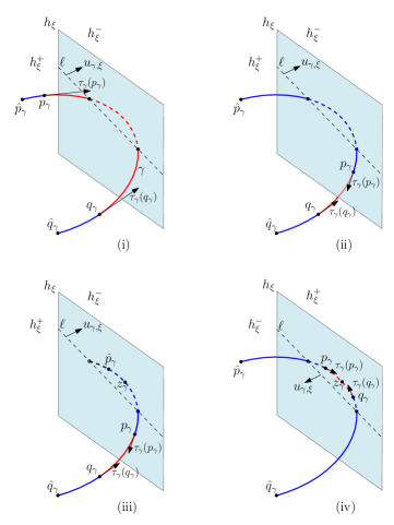
Figure 3: Illustration of the proof of Lemma 4.2; (i) $\gamma$ intersects $h_{\xi}$, (ii) one arc of $\hat{\gamma}\setminus\gamma$ contains both intersection points of $\hat{\gamma}\cap h_{\xi}$, (iii) each of the arcs of $\hat{\gamma}\setminus\gamma$ contains at most one intersection point of $\hat{\gamma}\cap h_{\xi}$ and $z_{\gamma}\in h_{\xi}^{-}$, and (iv) $z_{\gamma}\in h_{\xi}^{+}$.

Lemma 4.2.

The arc $\gamma$ intersects $h_{\xi}$ if and only if (a) both $\tau_{\gamma}(p_{\gamma})$ and $\tau_{\gamma}(q_{\gamma})$ point toward $h_{\xi}$, and (b) $\hat{\gamma}$ intersects $h_{\xi}$. See Figure 3.

Proof.

Assume first that $\gamma$ intersect $h_{\xi}$. Property (b) holds trivially, so it suffices to prove that (a) also holds. Since $p_{\gamma}$ and $q_{\gamma}$ lie on the same side of the line $\ell$, $\gamma\cap h_{\xi}^{-}$ contains a point $z_{\gamma}$ at which the tangent to $\gamma$ is parallel to $\ell$ (and thus normal to the vector $u_{\gamma,\xi}$). For a point $z\in\gamma$, let $\overrightarrow{\tau}(z)$ be the tangent of $c_{\gamma}$ at $z$ oriented in clockwise direction (i.e., toward $q_{\gamma}$). For $z=p_{\gamma}$, $\overrightarrow{\tau}(p_{\gamma})=\tau_{\gamma}(p_{\gamma})$. Since $z_{\gamma}\in h_{\xi}^{-}$, if we trace $z$ back from $z_{\gamma}$ toward the initial point $p_{\gamma}$, the angle between $\overrightarrow{\tau}(z)$ and $u_{\gamma,\xi}$, measured counterclockwise from $\overrightarrow{\tau}(z)$ to $u_{\gamma,\xi}$, decreases from $+\pi/2$, so $z$ has to turn by more than $\pi$ till $\overrightarrow{\tau}(z)$ forms an obtuse angle with $u_{\gamma,\xi}$. But $\gamma$ turns by at most $\pi$, as it is contained in one of the canonical semi-circles of $c_{\gamma}$. Hence, $p_{\gamma}$ points toward $h_{\xi}$. A similar argument shows that $q_{\gamma}$ also points toward $h_{\xi}$, thereby establishing (a).

Conversely, assume that (a) and (b) hold but $\gamma$ does not cross $h_{\xi}$, i.e., $\gamma\subset h_{\xi}^{+}$. Then $\hat{\gamma}\setminus\gamma$ intersects $h_{\xi}$ in one or two points. Assume that $\hat{\gamma}\setminus\gamma$ consists of two arcs $\gamma^{-}$ and $\gamma^{+}$, which are the respective portions of $\hat{\gamma}$ between $p_{\hat{\gamma}}$ and $p_{\gamma}$ and between $q_{\gamma}$ and $q_{\hat{\gamma}}$. (If one of the arcs is empty, then the argument is simpler.) Assume first that one of these two arcs, say, $\gamma^{-}$, intersects $h_{\xi}$ at two points. Then the above argument implies that $\tau_{\gamma^{-}}(p_{\gamma})$ points toward $h_{\xi}$, which implies that $\tau_{\gamma}(p_{\gamma})=-\tau_{\gamma^{-}}(p_{\gamma})$ points away from $h_{\xi}$, thereby contradicting (a). A similar contradiction occurs if $\gamma^{+}$ intersects $h_{\xi}$ twice.

Assume then that each of $\gamma^{-},\gamma^{+}$ intersects $h_{\xi}$ at most once, and one of them intersects $h_{\xi}$ exactly once. Let $z_{\gamma}$ be the point on $\hat{\gamma}$ at which the tangent to $c_{\gamma}$ is parallel to $\ell$. Since $c_{\gamma}$ intersects $h_{\xi}$, the outer normal of $c_{\gamma}$ at $z_{\gamma}$ is $u_{\xi,\gamma}$ if $z_{\gamma}\in h_{\xi}^{-}$ and $-u_{\xi,\gamma}$ otherwise. Assume first that $z_{\gamma}\in h_{\xi}^{-}$, in which case the outer normal at $z_{\gamma}$ is $u_{\xi,\gamma}$ and $z_{\gamma}\in\hat{\gamma}\setminus\gamma$. Suppose $z_{\gamma}\in\gamma^{-}$. As above, for a point $z\in\gamma^{-}$, let $\overrightarrow{\tau}(z)$ be the tangent of $c_{\gamma}$ at $z$ oriented in clockwise direction (toward $p_{\gamma}$). Note that $\overrightarrow{\tau}(p_{\gamma})=\tau_{\gamma}(p_{\gamma})$ and the angle between $u_{\xi,\gamma}$ and $\overrightarrow{\tau}(z_{\gamma})$ is $\pi/2$. As we trace $z$ forward from $z_{\gamma}$ toward $p_{\gamma}$, the angle between $u_{\xi,\gamma}$ and $\overrightarrow{\tau}(z)$ increases. Since $\gamma^{-}$ turns by at most $\pi$, $\overrightarrow{\tau}(p_{\gamma})$ makes an obtuse angle with $u_{\xi,\gamma}$, i.e., $\tau_{\gamma}(p_{\gamma})$ points away from $h_{\xi}$, contradicting condition (a). A similar contradiction can be attained if $z_{\gamma}\in\gamma^{+}$.

Next, assume that $z_{\gamma}\in h_{\xi}^{+}$, in which case the outer normal of $c_{\gamma}$ at $z_{\gamma}$ is $-u_{\xi,\gamma}$. We note that either $p_{\gamma}$ lies between $p_{\hat{\gamma}}$ and $z_{\gamma}$ (if $z_{\gamma}\in\gamma\cup\gamma^{+}$), or $q_{\gamma}$ lies between $z_{\gamma}$ and $q_{\hat{\gamma}}$ (if $z_{\gamma}\in\gamma^{-}\cup\gamma$); both conditions hold if $z_{\gamma}\in\gamma$. Without loss of generality, assume that $p_{\gamma}$ appears between $p_{\hat{\gamma}}$ and $z_{\gamma}$. Let $\overrightarrow{\tau}(z)$ be the same as above; again, $\overrightarrow{\tau}(p_{\gamma})=\tau_{\gamma}(p_{\gamma})$. As we trace $z$ backward (in counterclockwise direction) from $z_{\gamma}$ toward $p_{\gamma}$, the angle between $\overrightarrow{\tau}(z)$ and $u_{\gamma,\xi}$, which at $z_{\gamma}$ is $\pi/2$, increases. Since $\gamma$ turns by at most $\pi$, we can conclude that the angle between $u_{\xi,\gamma}$ and $\overrightarrow{\tau}(p_{\gamma})$ is obtuse, i.e., $p_{\gamma}$ points away from $h_{\xi}$. A similar argument shows that if $z_{\gamma}$ lies before $p_{\gamma}$ (in which case $q_{\gamma}$ lies between $z_{\gamma}$ and $q_{\hat{\gamma}}$), then $q_{\gamma}$ points away from $h_{\xi}$.

Since condition (a) is violated in all cases, we conclude that $\gamma$ intersects $h_{\xi}$. ∎

In view of Lemma 4.2 and the discussion in Section 3.4, the condition that $\gamma$ intersects the pseudo-trapezoid $\varphi\in\Phi_{C}$, under the setup in Case (i), can be described as:

• The endpoints $p_{\gamma}$ and $q_{\gamma}$ lie on the same side of $h_{\xi}$;

• both $\tau_{\gamma}(p_{\gamma})$ and $\tau_{\gamma}(q_{\gamma})$ point toward $h_{\xi}$; and

• $\Pi_{C}(\hat{\gamma},\xi)=1$, where $\Pi_{C}$ is the predicate defined in (9).

Each of these conditions can be expressed as a constant-size semi-algebraic predicate in which each polynomial inequality uses at most six parameters of $\gamma$: Condition (i) needs three parameters, condition (ii) needs four parameters—two to describe the tangent vector $\tau_{\gamma}(p_{\gamma})$ (or $\tau_{\gamma}(q_{\gamma})$) and two to denote the normal of $\pi_{\gamma}$ (which is needed to specify $u_{\gamma,\xi}$), and condition (iii) needs six parameters to describe $\hat{\gamma}$.

Case (ii): $p_{\gamma},q_{\gamma}$ lie on opposite sides of $h_{\xi}$.

In this case $\gamma$ intersects $h_{\xi}$ at exactly one point, say, $w_{\gamma}$. But the semi-circle $\hat{\gamma}$ may intersect $h_{\xi}$ also at another point. There are three subcases depending on the halfplanes of $h_{\xi}$ that contain the endpoints $p_{\hat{\gamma}}$ and $q_{\hat{\gamma}}$ of $\hat{\gamma}$ (which also determines how many times $\hat{\gamma}$ intersects $h_{\xi}$).

Case (ii.a): $p_{\hat{\gamma}}$ and $q_{\hat{\gamma}}$ lie on opposite sides of $h_{\xi}$. Since $\gamma\subseteq\hat{\gamma}$, $p_{\gamma}$ and $p_{\hat{\gamma}}$ lie on the same side of $h_{\xi}$, and $q_{\gamma}$ and $q_{\hat{\gamma}}$ lie on the other side. Furthermore $w_{\gamma}$ is the only intersection point of $\hat{\gamma}$ and $h_{\xi}$. Therefore $\gamma$ intersects the pseudo-trapezoid $\varphi$ if and only if $\hat{\gamma}$ intersects $\varphi$, and the intersection condition for this case can be specified as:

1. $p_{\gamma},q_{\gamma}$ lie on opposite sides of $h_{\xi}$;

2. $p_{\gamma}$ and $p_{\hat{\gamma}}$ lie in the same halfplane of $h_{\xi}$, and the same holds for $q_{\gamma}$ and $q_{\hat{\gamma}}$; and

3. $\Pi_{C}(\hat{\gamma},\xi)=1$.

Case (ii.b): $p_{\hat{\gamma}}$ and $q_{\hat{\gamma}}$ lie on same side of $h_{\xi}$ as $p_{\gamma}$. In this case $\hat{\gamma}$ intersects $h_{\xi}$ at two points, one of which is $w_{\gamma}$. Let $\bar{w}_{\gamma}$ be the other intersection point. Since $p_{\gamma}$ and $p_{\hat{\gamma}}$ lie in the same halfplane of $h_{\xi}$, $\bar{w}_{\gamma}$ lies on $\hat{\gamma}$ between $q_{\gamma}$ and $q_{\hat{\gamma}}$. That is, assuming that $\hat{\gamma}$ is oriented from $p_{\hat{\gamma}}$ to $q_{\hat{\gamma}}$, $w_{\gamma}$ is the first intersection point of $\hat{\gamma}$ with $h_{\xi}$ and $\bar{w}_{\gamma}$ is the second one. In order to detect whether $\gamma$ intersects the pseudo-trapezoid $\varphi$, unlike the previous case, we cannot simply use the predicate $\Pi_{C}(\hat{\gamma},\xi)$, because $\bar{w}_{\gamma}$ might lie in $\varphi$ while $w_{\gamma}$ does not. Hence, we use the extension $\Pi_{C}^{(1)}(\hat{\gamma},\xi)$ of $\Pi_{C}(\hat{\gamma},\xi)$, defined in Remark 2 (cf. Section 3.4), which asserts that the first intersection point of $\hat{\gamma}$, which is $w_{\gamma}$, lies in $\varphi$. The intersection condition can now be expressed as:

1. $p_{\gamma},q_{\gamma}$ lie on opposite sides of $h_{\xi}$;

2. both $p_{\hat{\gamma}}$ and $q_{\hat{\gamma}}$ lie in the same halfplane of $h_{\xi}$ as $p_{\gamma}$; and

3. $\Pi_{C}^{(1)}(\hat{\gamma},\xi)=1$.

Figure 4: An instance where only the second crossing point of $\hat{\gamma}$ with $h_{\Delta}$ lies in $C$ but this point does not belong to $\gamma$.

Case (ii.c): $p_{\hat{\gamma}}$ and $q_{\hat{\gamma}}$ lie on same side of $h_{\xi}$ as $q_{\gamma}$. This case is symmetric to the previous case, except that $\bar{w}_{\gamma}$ now lies between $p_{\hat{\gamma}}$ and $p_{\gamma}$ on $\hat{\gamma}$. To handle this case we simply reverse the direction of $\hat{\gamma}$, and use the same analysis as in the previous case.

In summary, the intersection condition between $\gamma$ and $\varphi$ in each of the three subcases of case (ii) is specified as a constant-complexity semi-algebraic predicate in which each polynomial inequality uses at most six parameters of $\gamma$. Combining with case (i), we thus conclude that the intersection condition between a circular arc and a pseudo-trapezoid of $\Phi_{C}$ can be written as a disjunction of four constant-complexity conjunctions, so that each polynomial inequality in each of them uses at most six of the eight (real) parameters specifying $\gamma$. Hence, by building a multi-level point-enclosure-query data structure for each case separately, we can construct a data structure of size $O^{*}(n^{6})$ that can answer an intersection query on $\Phi_{C}$ in $O^{*}(1)$ time. Using the standard technique for space/query-time trade-off, sketched in Section 4.1 (see also Appendix A.2), for a given storage parameter $s\in[n,n^{6}]$, an intersection query can be answered in $O\left((n^{6}/s)^{2/15}\right)=O^{*}\left(n^{4/5}/s^{2/15}\right)$ time. Putting everything together, we obtain the following result.

Lemma 4.3.

Let $\mathscr{W}$ be a set of $n$ wide plates at some cell $\tau$ of $\mathbb{R}^{3}\setminus Z(F)$, and let $n\leq s\leq n^{6}$ be a prespecified storage parameter. $\mathscr{W}$ can be preprocessed, in $O^{*}(s)$ expected time, into a data structure of size $O^{*}(s)$, so that an intersection query on $\mathscr{W}$ within $\tau$ with a circular arc in $\mathbb{R}^{3}$ can be answered in $O^{*}(n^{4/5}/s^{2/15})$ time.

4.3 The case of planar query arcs

We now let $\Gamma$ be a family of arbitrary constant-degree planar algebraic arcs. The machinery presented in Section 4.2 for circular arcs also works, with minor modifications, for intersection queries with arbitrary constant-degree planar algebraic arcs. To obtain this extension, we first break the curve $\sigma_{\gamma}$ containing the query arc $\gamma$, and $\gamma$ too if needed, at its $O(1)$ inflection points, and also at a constant number of additional points, so that the turning angle of each resulting portion of the curve is at most $\pi$. The overall number of these breakpoints is linear in the degree of $\gamma$.

By construction, each of these portions is a convex arc. We then apply the intersection-searching algorithm to each portion separately. Since each portion is convex, it can intersect a plane in at most two points. The algorithm presented above for circular arcs, and its analysis, easily extends to such general arcs, with suitable and straightforward modifications; the routine details are omitted.

Let $t$ be the reduced parametric dimension of the curves supporting the query arcs. Following the same analysis as above, for a storage parameter $s\in[n,n^{t}]$, an intersection query on $\mathscr{W}$ (within $\tau$) can be answered in $O^{*}\left((n^{t}/s)^{{\tfrac{2}{3(t-1)}}}\right)$ time, using an $O^{*}(s)$-size data structure:

Lemma 4.4.

Let $\mathscr{W}$ be a set of $n$ wide plates at some cell $\tau$ of $\mathbb{R}^{3}\setminus Z(F)$, let $\Gamma$ be a family of constant-degree planar algebraic arcs such that their supporting curves have constant reduced parametric dimension $t\geq 3$ (with respect to $\mathscr{W}$). Let $n\leq s\leq n^{t}$ be a prespecified storage parameter. $\mathscr{W}$ can be preprocessed, in $O^{*}(s)$ expected time, into a data structure of size $O^{*}(s)$, so that an intersection query on $\mathscr{W}$ within $\tau$ with an arc in $\Gamma$ can be answered in $O^{*}\left((n^{t}/s)^{\tfrac{2}{3(t-1)}}\right)$ time.

5 Space/Query-Time Trade-Offs for the Overall Data Structure

We are now ready to describe how we adapt the data structure described in Section 2 to obtain space/query-time trade-offs for arc-intersection queries. As above, let $\mathscr{T}$ be the set of input plates, and let $\Gamma$ be the family of query arcs. Let ${t_{o}}$ be the reduced parametric dimensions of $\mathscr{T}$ (relative to $\Gamma$), and let ${t_{q}}$ be the reduced parametric dimension of $\Gamma$, respectively. Given a storage parameter $s\in[n,n^{{t_{q}}}]$, we construct, in $O^{*}(s)$ expected time, a data structure of size $O^{*}(s)$, that can answer an arc-intersection query in time

$$O^{*}\left(\frac{n^{2-3/{t_{o}}}}{s^{1-2/{t_{o}}}}+\left(\frac{n^{{t_{q}}}}{s}\right)^{\tfrac{2}{3({t_{q}}-1)}}\right).$$

We present two data structures: the first one is used for $s\in[n,n^{3/2}]$, and we refer to it as a moderate-size data structure. The second one, called a large-size data structure, is used for $s\in[n^{3/2},n^{{t_{q}}}]$, and uses the moderate-size data structure as a substructure.

5.1 Moderate-size data structure

For $n\leq s\leq n^{3/2}$, we build the same partition tree $\Psi$ as described in Section 2.1 but with a few twists. Let $D>0$ be a sufficiently large constant parameter as before. First, the recursive subproblem at a node $v$ of $\Psi$ involves two parameters: a subset $\mathscr{T}_{v}\subseteq\mathscr{T}$ of plates of size $n_{v}$ (as before), and a storage parameter $s_{v}\geq n_{v}$ that specifies, in the asymptotic $O^{*}(\cdot)$ sense, the size of the subtree $\Psi_{v}$ constructed at $v$. Initially, at the root, $\mathscr{T}_{v}=\mathscr{T}$ and $s_{v}=s$. Second, we set the threshold value $n_{0}$ for termination of the recursion to be

$$n_{0}=n^{3}/s^{2};$$

note that $n_{0}\geq 1$ for $s\leq n^{3/2}$.

If $n_{v}\leq n_{0}$, we construct a data structure (multi-level partition tree) of $O^{*}(n_{v})$ size, as described in Section 2.3. If $n_{v}>n_{0}$, we construct a partitioning polynomial $F_{v}$ of degree at most $c_{1}D$, for a suitable absolute constant $c_{1}$, and the secondary data structures $\Sigma_{v}$ and $\varUpsilon_{v}$ to handle the query arcs that are contained in $Z(F_{v})$ and to answer intersection queries for wide plates, respectively, as before. However the size of each of $\Sigma_{v},\varUpsilon_{v}$ is now $O^{*}(s_{v})$, which allows a query to be answered faster. We already have described in Section 4 how to construct $\varUpsilon_{v}$ for a given storage parameter $s_{v}$, and we describe a similar construction of $\Sigma_{v}$ in Section 6 (see Lemma 6.2).

Finally, for each cell $\tau$ of $\mathbb{R}^{3}\setminus Z(F_{v})$, we recursively construct the data structure on the subset $\mathscr{T}_{\tau}\subset\mathscr{T}_{v}$ with storage parameter set to $s_{v}/D^{3}$.

An intersection query with an arc $\gamma\in\Gamma$ is answered as described in Section 2.2, except that we use the procedures described in Sections 4 and 6 to query the respective secondary data structure $\varUpsilon_{v}$ and $\Sigma_{v}$ at each node $v$.

Let $S(n_{v},s_{v})$ denote the maximum size of the subtree $\Psi_{v}$, and let $Q(n_{v},s_{v})$ denote the maximum query time on $\Psi_{v}$. We obtain the following recurrence for $S(n_{v},s_{v})$:

$$S(n_{v},s_{v})\leq\begin{cases*}\displaystyle c_{2}D^{3}S\left(\frac{n_{v}}{D^{2}},\frac{s_{v}}{D^{3}}\right)+c_{3}s_{v}n_{v}^{\delta}&for $n_{v}>n_{0}$,\\[2.84526pt] c_{4}n_{v}^{1+\delta}&for $n_{v}\leq n_{0}$,\end{cases*}$$ (11)

where $c_{2},c_{3},c_{4}$, and $\delta$ are constants as defined in Section 2.1. Using induction on $n_{v}$, as in Section 2.1, we can show that the solution to the recurrence is

$$S(n_{v},s_{v})\leq A\left(s_{v}+s\left(\frac{n_{v}}{n}\right)^{3/2}\right)n_{v}^{\varepsilon}$$ (12)

for any $\varepsilon>\delta$, provided the constants $A$ and $D$ are chosen sufficiently large. Roughly speaking, by the choice of the storage parameters for each subproblem, the secondary data structures use $O^{*}(s_{v})$ storage at each level of $\Psi$. Furthermore, there are $O^{*}((n_{v}/n_{0})^{3/2})$ leaves of $\Psi$, each of which uses $O^{*}(n_{0})$ space. Since $n_{0}=n^{3}/s^{2}$, the total space used at the leaves of $\Psi$ is $O^{*}((n_{v}/n)^{3/2}s)$. Hence, the overall size of $\Psi$ is $S(n,s)=O^{*}(s)$.

Concerning the query cost, by adapting (4) and plugging the query-time bounds for the secondary data structures from Lemmas 4.4 and 6.2, we obtain the following recurrence:

$$Q(n_{v},s_{v})\leq\begin{cases*}\displaystyle c_{5}DQ\left(\frac{n_{v}}{D^{2}},\frac{s_{v}}{D^{3}}\right)+c_{6}\left(\frac{n_{v}^{{t_{q}}}}{s_{v}}\right)^{\frac{2}{3({t_{q}}-1)}}n_{v}^{\delta}&for $n_{v}>n_{0}$,\\[2.84526pt] c_{7}n_{v}^{1-\tfrac{1}{{t_{o}}}+\delta}&for $n_{v}\leq n_{0}$,\end{cases*}$$ (13)

where $c_{5},c_{6},c_{7}$ and $\delta$ are constants as defined in Section 2.2. For our choice of storage parameter, (13) implies that the time spent in querying the secondary structures at the children of a node $v$, namely the sum of the nonrecursive overhead terms at the children, is $c_{5}D^{\tfrac{3-{t_{q}}}{3({t_{q}}-1)}}$ times the cost at $v$. Therefore, for ${t_{q}}\geq 3$, the total time spent in querying the secondary data structures at all levels is $O^{*}\biggl{(}(n_{v}^{{t_{q}}}/s_{v})^{\tfrac{2}{3({t_{q}}-1)}}\biggr{)}$. Furthermore, the procedure visits $O^{*}(s/n)$ leaves and spends $O^{*}(n_{0}^{1-1/{t_{o}}})$ time at each of them. Recalling our choice of $n_{0}$, summing these bounds, and setting $n_{v}=n$ and $s_{v}=s$, we obtain that the overall query time is

$$Q(n,s)=O^{*}\left(\frac{n^{2-3/{t_{o}}}}{s^{1-2/{t_{o}}}}+\left(\frac{n^{{t_{q}}}}{s}\right)^{\tfrac{2}{3({t_{q}}-1)}}\right).$$ (14)

In particular, for $s=n^{3/2}$, the query time is $O^{*}\biggl{(}n^{\tfrac{2{t_{q}}-3}{3({t_{q}}-1)}}\biggr{)}$. This is because this term dominates the first term in (14), which is $O^{*}(n^{1/2})$ when $s=n^{3/2}$, as long as ${t_{q}}\geq 3$. If $\Gamma$ is a family of planar arcs, then ${t_{q}}$ is the reduced parametric dimension of the curves supporting the arcs in $\Gamma$.

5.2 The large-size data structure

We now assume that $s\in[n^{3/2},n^{{t_{q}}}]$. As in Section 4.1, for simplicity, we assume that ${t_{q}}$ is also the parametric dimension of $\Gamma$. See Appendix A for the general case when ${t_{q}}$ is smaller than the dimension of the query space. Each plate $\Delta$ in $\mathscr{T}$ can be mapped to a constant-complexity semi-algebraic region $\widetilde{\Delta}$ in the query space $\mathbb{R}^{{t_{q}}}$, so that an arc $\gamma\in\Gamma$ intersects $\Delta$ if and only if $\gamma^{*}\in\widetilde{\Delta}$. Let $\widetilde{\mathscr{T}}\coloneqq\{\widetilde{\Delta}\mid\Delta\in\mathscr{T}\}$. We now set a threshold value $n_{0}\coloneqq\left(n^{{t_{q}}}/s\right)^{\tfrac{1}{{t_{q}}-3/2}}$. The data structure is almost the same as the one described in Section 4.1, except that (a) if the value of the storage parameter at a node $v$ is $s_{v}$, the parameter allocated to each of its children is $s_{v}/D^{{t_{q}}}$, and (b) at each “leaf” node we build the moderate-size data structure just described (in Section 5.1) on the plates associated with that leaf, with storage parameter $n_{0}^{3/2}$. The query procedure is also the same, except that we use the procedure for the moderate-size data structure to answer a query at a leaf.

Concretely, by the analysis in Section 4.1, the storage used by the structure is $O^{*}((n/n_{0})^{{t_{q}}}s(n_{0}))$, where $s(n_{0})=n_{0}^{3/2}$ is the storage parameter at a leaf. That is, by our choice of $n_{0}$, the storage is

$$O^{*}\left(\biggl{(}\frac{n}{n_{0}}\biggr{)}^{{t_{q}}}n_{0}^{3/2}\right)=O^{*}\left(\frac{n^{{t_{q}}}}{n_{0}^{{t_{q}}-3/2}}\right)=O^{*}(s).$$

Following the same analysis as in Section 4.1, see also Appendix A, the query time is (within $n^{\varepsilon}$ factor) the same as the time spent at a leaf, which is

$$O^{*}\biggl{(}n_{0}^{\tfrac{2{t_{q}}-3}{3({t_{q}}-1)}}\biggr{)}=O^{*}\left(\left(\frac{n^{{t_{q}}}}{s}\right)^{\frac{2}{3({t_{q}}-1)}}\right).$$

Hence, we conclude that the overall query time is is $O^{*}\biggl{(}(n^{{t_{q}}}/s)^{\tfrac{2}{3({t_{q}}-1)}}\biggr{)}$. If the arcs in $\Gamma$ are planar, then as in Section 4.3, ${t_{q}}$ is the reduced parametric dimension of the curves supporting the arcs of $\Gamma$. Combining this with the bound (14) for the moderate-size case, we obtain the following result.

Theorem 5.1.

Let $\Gamma$ be a family of parametrized algebraic arcs of constant complexity, let $\mathscr{T}$ be a set of $n$ plates in $\mathbb{R}^{3}$, let ${t_{o}}$ be the reduced parametric dimension of $\mathscr{T}$, let ${t_{q}}$ be the reduced parametric dimension of $\Gamma$ or of the curves supporting the arcs in $\Gamma$ if they are planar, and let $s\in[n,n^{{t_{q}}}]$ be a storage parameter. $\mathscr{T}$ can be preprocessed, in expected time $O^{*}(s)$, into a data structure of size $O^{*}(s)$, so that an arc-intersection query amid the plates of $\mathscr{T}$ with an arc in $\Gamma$ can be answered in time

$$O^{*}\left(\frac{n^{2-3/{t_{o}}}}{s^{1-2/{t_{o}}}}+\left(\frac{n^{{t_{q}}}}{s}\right)^{\tfrac{2}{3({t_{q}}-1)}}\right).$$

Remark 3.

Theorem 5.1 is obtained by combining three data structures: (D1) the polynomial partitioning method described in Section 2 that is constructed in $\mathbb{R}^{3}$, (D2) the linear-size semi-algebraic partition tree of [40] that is constructed in the object space, and (D3) the semi-algebraic point-enclosure data structure of [8] that is constructed in the query space. However, for any specific value of $s$, only two of these data structures are actually combined: For $s\leq n^{3/2}$, the moderate-size data structures combines (D1) with (D2). For $s>n^{3/2}$, the large-size data structure first builds (D3), and then constructs an instance of (D1) at each leaf of (D3) with storage parameter $n_{0}^{3/2}$, where $n_{0}$ is the size of the subproblem at the leaf. With this choice of the storage parameter, (D1) is recursively constructed until the size of the subproblem falls below a constant, and thus (D2) is never constructed at a leaf of (D1).

If $\mathscr{T}$ is a set of $n$ triangles in $\mathbb{R}^{3}$, then ${t_{o}}=5$ for general algebraic arcs (namely, this is the best bound we have so far) and ${t_{o}}=4$ for lines; ${t_{q}}=4$ in the latter case. We thus obtain the following corollary.

Corollary 5.2.

Let $\mathscr{T}$ be a set of $n$ triangles in $\mathbb{R}^{3}$, let $\Gamma$ be a family of parametrized algebraic arcs. Let ${t_{q}}$ be the reduced parametric dimension of $\Gamma$ or of the curves supporting the arcs of $\Gamma$ if they are planar, and let $s\in[n,n^{{t_{q}}}]$ be a storage parameter. $\mathscr{T}$ can be preprocessed, in $O^{*}(s)$ expected time, into a data structure of size $O^{*}(s)$, so that an intersection query with an arc in $\Gamma$ can be answered in $O^{*}\biggl{(}n^{7/5}/s^{3/5}+(n^{{t_{q}}}/s)^{\tfrac{2}{3({t_{q}}-1)}}\biggr{)}$ time. If $\Gamma$ is a set of line segments, then an intersection query can be answered in $O^{*}\left(n^{5/4}/s^{1/2}+(n^{4}/s)^{2/9}\right)$ time, for $s\in[n,n^{4}]$.

6 Handling the Zero Set

Let $\Gamma$ and $\mathscr{T}$ be as above, and let $F$ be a partitioning polynomial of degree at most $D$, for some constant $D>0$, as described in Section 2. We assume that no plate in $\mathscr{T}$ lies in $Z(F)$, i.e., the intersection of a plate with $Z(F)$ is a collection of algebraic arcs, all contained in a single algebraic curve (of constant degree). This assumption is justified because, by assumption, $Z(F)$ (or rather its planar components) contains only $O(1)$ input plates, which are handled separately; see Section 2.1. In this section, we present a data structure for answering intersection queries amid $\mathscr{T}$ with an arc $\gamma\in\Gamma$ that is contained in $Z(F)$.

Our data structure is based on a hierarchical polynomial-partitioning technique proposed in [8] (cf. Lemma A.2 in the appendix). For a subset $\mathscr{X}\subseteq\mathscr{T}$ and a parameter $E\gg D$, this technique constructs a partitioning polynomial $G\in\mathbb{R}[x,y,z]$ of degree at most $c^{\prime}_{1}E$, for a constant $c^{\prime}_{1}>0$ that depends (polynomially) on $D$, such that any cell of $\mathscr{A}(G;F)$, which is the decomposition of $Z(F)$ induced by $Z(G)$, that does not lie in $Z(G)$ (i.e., a cell of $Z(F)\setminus Z(G)$) is crossed by at most $m/E$ plates of $\mathscr{X}$, and contains at most $m/E^{2}$ endpoints of the intersection arcs of $\mathscr{X}$ and $Z(F)$. The number of cells in $\mathscr{A}(G;F)$ is at most $c^{\prime}_{2}E^{2}$, for a constant $c^{\prime}_{2}>0$ (that depends on $D$). With this polynomial partitioning at our disposal, we build a data structure similar to the one presented in Section 2.1. Namely, we construct a partition tree $\Sigma$ on $\mathscr{T}$. Each node of $\Sigma$ stores a secondary data structure, analogous to the one in Section 3, to handle wide plates at the corresponding cell. We describe the overall data structure briefly, highlighting the differences from the earlier structure.

6.1 Overall data structure

Each node $z\in\Sigma$ is associated with a constant-size semi-algebraic cell $\sigma_{z}\subseteq Z(F)$ and a subset $\mathscr{T}_{z}\subseteq\mathscr{T}$ of $n_{z}$ plates. If $z$ is the root of $\Sigma$, then $\sigma_{z}=Z(F)$ and $\mathscr{T}_{z}=\mathscr{T}$. Set $n_{z}=|\mathscr{T}_{z}|$. We fix two sufficiently large constants $n_{1}\geq 0$ (a threshold parameter) and $E=D^{O(1)}$.

If $n_{z}\leq n_{1}$ then $z$ is a leaf and we simply store $\mathscr{T}_{z}$ at $z$. Otherwise, we construct a partitioning polynomial $G_{z}$ for $\mathscr{T}_{z}$ (relative to $F$) of degree at most $c^{\prime}_{1}E$, as described above, and store $G_{z}$ at $z$. By our general-position assumption on the input plates stated in Section 2—only $O(1)$ plates lie in any plane and any line is contained in supporting planes of $O(1)$ input plates—there are only $O(1)$ input plates for which $\dim(\Delta\cap Z(F)\cap Z(G))=1$. Let $\mathscr{T}_{z}^{0}\subseteq\mathscr{T}_{z}$ be the subset of these plates. We store $\mathscr{T}_{z}^{0}$ at $z$. Let $\sigma$ be a one- or two-dimensional cell of $\mathscr{A}(G;F)$. If $\sigma$ is a one-dimensional cell, which is a connected arc of the intersection curve $Z(G)\cap Z(F)$, we compute the set $\mathscr{T}_{\sigma}\subseteq\mathscr{T}_{z}\setminus\mathscr{T}_{z}^{0}$ of plates that intersect $\sigma$. Note that $\dim(\Delta\cap Z(F)\cap Z(G))=0$ for all $\Delta\in\mathscr{T}_{\sigma}$. Using a one-dimensional range-searching data structure, we preprocess $\mathscr{T}_{\sigma}$ into a linear-size data structure $\Sigma^{0}_{\sigma}$ that supports intersection queries for $\gamma\cap\sigma$, $\gamma\in\Gamma$, in $O(\log n)$ time; see also Appendix A.1. We store $\Sigma^{0}_{\sigma}$ at $z$. (By building an appropriate one-dimensional data structure on $\mathscr{T}_{z}$ (including $\mathscr{T}_{z}^{0}$) for each irreducible component of the curve $Z(F)\cap Z(G)$, we can remove the assumption that a line is contained in the supporting planes of $O(1)$ input plates, but for simplicity, we stick to the data structure just described.)

Assume next that $\sigma$ is a two-dimensional cell. We classify the input plates crossing $\sigma$ into narrow and wide plates, as in Section 2.1. We create a child $u_{\sigma}$ of $z$ associated with $\sigma$. Let $\mathscr{W}_{\sigma}$ (resp., $\mathscr{T}_{\sigma}$) denote the set of the wide (resp., narrow) plates at $\sigma$. We construct a secondary data structure $\Upsilon^{0}_{\sigma}$ on $\mathscr{W}_{\sigma}$, as described in Section 6.2 below, for answering arc-intersection queries amid the plates of $\mathscr{W}_{\sigma}$ (for intersections that occur within $\sigma$) with the arcs of $\Gamma$ that lie in $Z(F)$. $\varUpsilon_{\tau}$ is stored at the child $u_{\sigma}$ of $z$. Finally, we set $\mathscr{T}_{u_{\sigma}}=\mathscr{T}_{\sigma}$, recursively construct a partition tree for $\mathscr{T}_{u_{\sigma}}$, and attach it as the subtree rooted at $u_{\sigma}$.

Let $S(n_{z})$ be the maximum size of the subtree $\Sigma_{z}$ constructed on a set of at most $n_{z}$ plates. For $n_{z}\leq n_{1}$, $S(n_{z})=n_{z}$. For $n_{z}>n_{1}$, Lemma 6.3 below implies that the secondary structure for handling wide plates require $O^{*}(n_{z})$ space. Therefore $S(n_{z})$ obeys the recurrence:

$$S(n_{z})\leq\begin{cases*}\displaystyle c^{\prime}_{2}E^{2}S\left(\frac{n_{z}}{E^{2}}\right)+c^{\prime}_{3}n_{z}^{1+\delta}&for $n_{z}\geq n_{1}$,\\[2.84526pt] n_{z}&for $n_{z}\leq n_{1}$,\end{cases*}$$ (15)

where $c^{\prime}_{2},c^{\prime}_{3},\delta$ are constants analogous to those in (2). The solution to the above recurrence is $S(n_{z})=O(n_{z}^{1+\delta})$ provided that $E$ is chosen sufficiently large. Hence, the overall size of $\Sigma$ is $O^{*}(n)$.

The query procedure is similar to Section 2.2. Using Lemma 6.3 again for the query cost amid the wide plates, we obtain the following recurrence for the query cost $Q(n_{z})$:

$$Q(n_{z})\leq\begin{cases*}\displaystyle c^{\prime}_{5}EQ\left(\frac{n_{z}}{E^{2}}\right)+c^{\prime}_{6}n_{z}^{2/3+\delta}&for $n_{z}\geq n_{1}$,\\[2.84526pt] n_{z}&for $n_{z}\leq n_{1}$,\end{cases*}$$ (16)

where $c^{\prime}_{5},c^{\prime}_{6},\delta$ are constants analogous to those in (4). The solution to the above recurrence is $Q(n_{z})=O^{*}(n_{z}^{2/3})$. Hence, we obtain the following result.

Lemma 6.1.

Let $\Gamma$ be a family of constant-degree parametrized algebraic arcs, let $\mathscr{T}$ be a set of $n$ plates of constant complexity in $\mathbb{R}^{3}$, and let $F$ be a partitioning polynomial of some constant degree $D$. $\mathscr{T}$ can be processed, in $O^{*}(n)$ expected time, into a data structure of $O^{*}(n)$ size, so that an arc-intersection query amid the plates of $\mathscr{T}$ with an arc in $\Gamma$ that lies in $Z(F)$ can be answered in $O^{*}(n^{2/3})$ time. The hidden constants and factors in the bound also depend on $D$.

To obtain a space/query-time trade-off, we proceed as in Section 5.2, ignoring the fact that the query arcs lie on $Z(F)$. We set the threshold value $n_{0}\coloneqq(n^{{t_{q}}}/s)^{\tfrac{1}{{t_{q}}-1}}$ where ${t_{q}}$ is the reduced parametric dimension of $\Gamma$ or of the curves supporting the arcs in $\Gamma$ if they are planar. When the size of the subproblem falls below the threshold $n_{0}$, we use the data structure just described (i.e., use Lemma 6.1). Following the same analysis as in Section 5.2, we obtain the following result.

Lemma 6.2.

Let $\Gamma$ be a family of constant-degree parametrized algebraic arcs, let $\mathscr{T}$ be a set of $n$ plates in $\mathbb{R}^{3}$, let ${t_{q}}$ be the reduced parametric dimension of arcs in $\Gamma$ or of the curves supporting the arcs in $\Gamma$ if they are planar, let $F$ be a partitioning polynomial of constant degree, and let $s\in[n,n^{{t_{q}}}]$ be a prespecified storage parameter. $\mathscr{T}$ can be preprocessed, in expected time $O^{*}(s)$, into a data structure of size $O^{*}(s)$, so that an arc-intersection query amid the plates of $\mathscr{T}$ with an arc in $\Gamma$ that lies in $Z(F)$ can be answered in $O^{*}\biggl{(}(n^{{t_{q}}}/s)^{\tfrac{2}{3({t_{q}}-1)}}\biggr{)}$ time.

6.2 Handling wide plates

Let $\mathscr{T}$, $\Gamma$, and $F$ be as above, and let $G\in\mathbb{R}[x,y,z]$ be a second partitioning polynomial (relative to $F$) as described above. In this subsection we present an algorithm for preprocessing the set $\mathscr{W}_{\sigma}$ of wide plates at a cell $\sigma$ of $Z(F)\setminus Z(G)$, for intersection queries (within $\sigma$) with the arcs of $\Gamma$ that lie in $Z(F)$. The high-level approach closely follows the approach of Section 3. It decomposes $\sigma\cap\Delta$, for $\Delta\in\mathscr{W}_{\sigma}$, into subarcs, and groups the resulting subarcs into $O(1)$ clusters, so that each cluster has an $O(1)$-size semi-algebraic encoding that depends only on the plane supporting $\Delta$ but not on its boundary. In this way, intersection searching for each cluster can be reduced to an instance of semi-algebraic range searching.

We now describe the algorithm in more detail, highlighting the differences from Section 3. Let $\mathbb{E}_{3}$ and $\mathbb{E}$ be the same as in Section 3. Define $\hat{F},\hat{G}\in\mathbb{R}[a,b,c,x,y]$ as $\hat{F}(a,b,c,x,y)=F(x,y,ax+by+c)$ and $\hat{G}(a,b,c,x,y)=G(x,y,ax+by+c)$. We construct a $5$-dimensional CAD $\hat{\Xi}$ of $\mathbb{E}$ induced by $\{\hat{F},\hat{G}\}$. Note that $\hat{\Xi}$ is a refinement of ${\Xi}$, the CAD constructed in Section 3 for $\hat{F}$. Here too, each cell of $\hat{\Xi}$ is given by a sequence of equalities or inequalities (one from each row) of the form in (3.2). Let $\hat{\Xi}_{3}$ denote the projection of $\hat{\Xi}$ onto $\mathbb{E}_{3}$, which we again refer to as the base of ${\Xi}$. We will be interested only in those cells of $\hat{\Xi}$ that lie in $Z(\hat{F})$, and we denote by $\hat{\Xi}_{F}$ the subset of these cells.

For a point $\xi=(a_{\xi},b_{\xi},c_{\xi})\in\mathbb{E}_{3}$, let $\hat{\Omega}(\xi)$ denote the $2$-dimensional fiber of $\hat{\Xi}$ over $\xi$ and $\hat{\Omega}^{\uparrow}(\xi)$ its lifting to the plane $h_{\xi}$. Again, we are interested only in the $1$-dimensional cells of $\hat{\Omega}^{\uparrow}(\xi)$ that lie in $Z(F)$. The combinatorial structure of $\hat{\Omega}(\xi)$, as well as of its lifting $\hat{\Omega}^{\uparrow}(\xi)$, remains the same for all points $\xi$ in the same base cell $\psi\in\hat{\Xi}_{3}$. As earlier, we associate each cell $\chi$ of $\hat{\Xi}_{F}$ with a fixed cell of $\mathscr{A}(G;F)$, denoted as $\sigma_{\chi}$, such that for all points $\xi$ in the base cell $\chi^{\downarrow}\in\hat{\Xi}_{3}$, $\chi^{\uparrow}(\xi)$ is an edge of $\hat{\Omega}^{\uparrow}(\xi)$ that lies in $\sigma_{\chi}$. For a cell $\chi\in\hat{\Xi}_{F}$ and a point $\xi\in\chi^{\downarrow}$, we use $\chi^{\uparrow}(\xi)$ to denote the arc of $\hat{\Omega}^{\uparrow}(\xi)$ corresponding to the cell $\chi$.

Let $\sigma$ be a $2$-cell of $\mathscr{A}(G;F)$. Let $\Delta\in\mathscr{W}_{\sigma}$ be a plate that is wide at $\sigma$, and let $\psi\in\hat{\Xi}_{3}$ be the base cell containing $\Delta^{*}$. We define $\Lambda_{\Delta,\sigma}$ to be the decomposition of $\Delta\cap\sigma$ into subarcs induced by $\hat{\Omega}^{\uparrow}(\Delta^{*})$, i.e.,

$$\Lambda_{\Delta,\sigma}\coloneqq\{\chi^{\uparrow}(\Delta^{*})\mid\chi\in\hat{\Xi}_{F},\,\Delta^{*}\in\chi^{\downarrow},\,\sigma_{\chi}=\sigma,\,\chi^{\uparrow}(\Delta^{*})\subseteq\Delta\cap Z(F)\}.$$

Set $\Lambda_{\sigma}=\bigcup_{\Delta\in\mathscr{W}_{\sigma}}\Lambda_{\Delta,\sigma}$, which is a decomposition of the set $\{\Delta\cap\sigma\mid\Delta\in\mathscr{W}_{\sigma}\}$ into subarcs induced by $\hat{\Xi}$. For a cell $\chi\in\hat{\Xi}_{F}$ with $\sigma_{\chi}=\sigma$, we define $\Lambda_{\chi}\subseteq\Lambda_{\sigma}$ to be the set of arcs defined by the cell $\chi\in\hat{\Xi}_{F}$, i.e.,

$$\Lambda_{\chi}=\{\chi^{\uparrow}(\Delta^{*})\mid\Delta\in\mathscr{W}_{\sigma}\;\wedge\;\chi^{\uparrow}(\Delta^{*})\in\Lambda_{\Delta,\sigma}\}.$$

By definition, $\Lambda_{\sigma}=\bigcup_{\chi\in\hat{\Xi}_{F}:\sigma_{\chi}=\sigma}\Lambda_{\chi}$. Let $\mathscr{T}_{\chi}\subseteq\mathscr{W}_{\sigma}$ be the set of plates corresponding to the arcs in $\Lambda_{\chi}$. All arcs in $\Lambda_{\chi}$ have a fixed constant-size semi-algebraic encoding of the form described in (8) that only depends on $F,G$ and the planes supporting them (but not on the boundary of the plates). Furthermore, the functions defining the encoding do not even depend on the supporting planes (whose coefficients only appear as variables in these functions). We can therefore define a $\chi$-intersection predicate $\breve{\Pi}_{\chi}\colon\Gamma\times\mathbb{E}_{3}\rightarrow\{0,1\}$, analogous to (9), such that $\breve{\Pi}_{\chi}(\gamma;\xi)=1$ if an intersection point of $\gamma$ and $h_{\xi}$ lies on the arc $\chi(\xi)$. That is,

$$\breve{\Pi}_{\chi}(\gamma;\xi)=\left\{\begin{array}[]{ll}1&\mbox{if }\xi\in\chi^{\downarrow}\wedge\exists(x_{p},y_{p},z_{p})\in\gamma\cap h_{\xi}\;\mbox{s.t.}\;(x_{p},y_{p})\in\chi(\xi),\\[2.84526pt] 0&\mbox{otherwise.}\end{array}\right.$$ (17)

This allows us to reduce the intersection searching on $\Lambda_{\chi}$ with an arc $\gamma\in\Gamma$ that is contained in $F$ to semi-algebraic range searching, for which we use the same data structures as in Section 3.4. Omitting all further details, we obtain the following result.

Lemma 6.3.

Let $\mathscr{W}$ be a set of $n$ wide plates for some $2$-cell $\sigma$ of $Z(F)\setminus Z(G)$, and let $\Gamma$ be a family of constant-degree parametrized algebraic arcs. $\mathscr{W}$ can be preprocessed, in $O^{*}(n)$ expected time, into a data structure of $O^{*}(n)$ size, so that an intersection query on $\mathscr{W}$ within $\sigma$ with an arc in $\Gamma$ that lies in $Z(F)$ can be answered in $O^{*}(n^{2/3})$ time.

7 Arc-Intersection Queries amid Triangles with Near-Linear Storage

In this section we describe a near-linear-size data structure for answering arc-intersection queries amid a set $\mathscr{T}$ of $n$ triangles in $\mathbb{R}^{3}$. Our main contribution is to show that, despite the default parametric dimension of a triangle in $\mathbb{R}^{3}$ being $9$ (which results, e.g., by specifying the coordinates of each of its three vertices), the reduced parametric dimension with respect to constant-degree parametrized algebraic arcs is only $5$, which immediately leads to an intersection-searching data structure with $O^{*}(n^{4/5})$ query time, using $O^{*}(n)$ space.

We represent a non-vertical triangle $\Delta$ in $\mathbb{R}^{3}$, with edges $e_{1},e_{2},e_{3}$, by the $9$-tuple $\Delta^{*}=(\xi,\mu,\nu)\in\mathbb{R}^{3}\times\mathbb{R}^{3}\times\mathbb{R}^{3}$, where $\xi$ is the point dual to the plane $h_{\Delta}$ supporting $\Delta$, and $\mu=(\mu_{1},\mu_{2},\mu_{3})\in\mathbb{R}^{3}$, $\nu=(\nu_{1},\nu_{2},\nu_{3})\in\mathbb{R}^{3}$ are defined so that, for $i=1,2,3$, $(\mu_{i},\nu_{i})$ specifies the line supporting the edge $e_{i}$ (within the plane $h_{\Delta}$). As in Section 3, we use $\mathbb{E}_{3}$ to denote the set of all non-vertical planes, each represented by its dual point. Recall that the family $\Gamma$ of query arcs is defined in Section 2 as follows:

$$\Gamma\coloneqq\{\gamma(\delta,\alpha^{-},\alpha^{+})\mid\delta\in\mathbb{E}_{t}\;\mbox{and}\;\alpha^{-},\alpha^{+}\in\mathbb{R}\},$$

where $t$ is the parametric dimension of curves supporting the arcs in $\Gamma$, and $\mathbb{E}_{t}$ is the $t$-dimensional parametric space of these curves.

Let $\Delta\in\mathscr{T}$ be a triangle, let $\gamma\coloneqq\gamma(\delta,\alpha^{-},\alpha^{+})\in\Gamma$ be an arc, and let $\sigma_{\delta}$ be the curve supporting the arc $\gamma$, where $\sigma_{\delta}(\alpha)=(x_{\delta}(\alpha),y_{\delta}(\alpha),z_{\delta}(\alpha))$ for $\alpha\in\mathbb{R}$. Then $\gamma$ intersects $\Delta$ if and only if (i) $\gamma$ intersects $h_{\Delta}$, and (ii) one of the intersection points of $\gamma\cap h_{\Delta}$ lies, within $h_{\Delta}$, on the positive side of each of the lines $\ell_{1}$, $\ell_{2}$, $\ell_{3}$ supporting the respective edges $e_{1}$, $e_{2}$, $e_{3}$ of $\Delta$, where the positive side of a line in $h_{\Delta}$ is the halfplane of $h_{\Delta}$ bounded by the line and containing $\Delta$. For technical reasons, we rewrite these conditions as follows:

There exists $\alpha\in\mathbb{R}$ such that

• $\sigma_{\delta}(\alpha)\in h_{\Delta}$.

• $\alpha^{-}\leq\alpha\leq\alpha^{+}$ (this sub-condition is vacuous when $\gamma$ is a full algebraic curve).

• $\sigma_{\delta}(\alpha)$ lies on the positive side of $\ell_{1}$.

• $\sigma_{\delta}(\alpha)$ lies on the positive side of $\ell_{2}$.

• $\sigma_{\delta}(\alpha)$ lies on the positive side of $\ell_{3}$.

A major technical issue that arises in expressing these conditions as semi-algebraic predicates is that $\sigma_{\delta}$ may intersect $h_{\Delta}$ in several points, and we need to test ($I_{2}$)–($I_{5}$) together for each intersection point separately. That is, for each of these tests, we need to specify which point (i.e., which value of $\alpha$) is to be used, and all four subpredicates ($I_{2}$)–($I_{5}$) must use the same value. More specifically, ($I_{1}$) gives $\alpha$ as a root of the algebraic equation $z_{\delta}(\alpha)=ax_{\delta}(\alpha)+by_{\delta}(\alpha)+c$, where $(a,b,c)$ are the coefficients of $h_{\Delta}$, and we need to specify which root to use in testing for conditions ($I_{2}$)–($I_{5}$).

To address this problem, we partition the product space $\mathbb{E}_{3}\times\mathbb{E}_{t}$ (in which a point $(\xi,\delta)$ corresponds to a pair of plane $h_{\xi}$ and curve $\sigma_{\delta}$) into $O(1)$ semi-algebraic regions such that for all pairs $(\xi,\delta)\in\mathbb{E}_{3}\times\mathbb{E}_{t}$ lying in the same region, the intersection points of the plane $h_{\xi}$ and the curve $\sigma_{\delta}$ have the same topological structure, and each of the intersection points has a fixed-size semi-algebraic encoding that is independent of $\xi$ and $\delta$. This encoding enables us to express each of the above conditions as a semi-algebraic predicate. We now describe the details.

Let $G\colon\mathbb{E}_{3}\times\mathbb{E}_{t}\times\mathbb{R}\rightarrow\mathbb{R}$ be the algebraic function

$$G(a,b,c;\delta;\alpha)\coloneqq z_{\delta}(\alpha)-ax_{\delta}(\alpha)-by_{\delta}(\alpha)-c,$$

where $x_{\delta},y_{\delta},z_{\delta}$ are the functions that define the curve $\sigma_{\delta}$ represented by the point $\delta\in\mathbb{R}^{t}$.

We construct a CAD ${\Xi}_{t+4}$ of $\mathbb{E}_{3}\times\mathbb{E}_{t}\times\mathbb{R}$ induced by $G$, where the order of coordinate elimination is first $\alpha$, then $\delta$, and then $c,b,a$. Each cell of ${\Xi}_{t+4}$ has a constant-size semi-algebraic representation analogous to (3.2).

Many of the technical details of the structure of ${\Xi}_{t+4}$ are similar to those used for the CAD introduced in Section 3, but we briefly sketch them because the setup is different here. Let ${\Xi}_{3}$ denote the projection of ${\Xi}_{t+4}$ onto the object space $\mathbb{E}_{3}$, and let ${\Xi}_{t+3}$ denote its projection onto the $(t+3)$-dimensional space $\mathbb{E}_{3}\times\mathbb{E}_{t}$. The latter gives the desired decomposition of the product space $\mathbb{E}_{3}\times\mathbb{E}_{t}$. For a cell $C\in{\Xi}_{t+4}$, let $C^{\Downarrow}$ (resp., $C^{\downarrow}$) denote its projection onto $\mathbb{E}_{3}$ (resp., onto $\mathbb{E}_{3}\times\mathbb{E}_{t}$). For each point $\xi\in\mathbb{E}_{3}$, denote by $\Omega^{t+1}(\xi)$ the $(t+1)$-dimensional fiber of ${\Xi}_{t+4}$ over $\xi$, and for each point $(\xi,\delta)\in\mathbb{E}_{3}\times\mathbb{E}_{t}$ denote by $\Omega^{1}(\xi,\delta)$ the one-dimensional fiber of ${\Xi}_{t+4}$ over $(\xi,\delta)$. Each $0$-dimensional cell (a point) in $\Omega^{1}(\xi,\delta)$ that lies in $Z(G)$ corresponds to (the value of $\alpha$ of) an intersection point of the curve $\sigma_{\delta}$ with the plane $h_{\xi}$. For all pairs $(\xi,\delta)$ in a cell $\psi\in{\Xi}_{t+3}$, $\Omega^{1}(\xi,\delta)$ has a fixed combinatorial structure. In particular, all of these pairs have the same number of $0$-dimensional cells in their fibers, and thus the same number of intersection points. Among the cells of ${\Xi}_{t+4}$ that lie in $Z(G)$ and in the cylinder over $\psi$, i.e., they project to $\psi$, the $i$-th cell, say, $C$, corresponds to the $i$-th intersection point of $\sigma_{\delta}\cap h_{\xi}$ for $(\xi,\delta)\in\psi$. Therefore the $i$-th intersection point of $\sigma_{\delta}$ abd $h_{\xi}$ (or rather the value of $\alpha$ corresponding to that point) has a fixed semi-algebraic encoding $\varphi_{C}(\xi;\delta)$ of constant complexity, which will be used for expressing the intersection condition.

Let ${\Xi}^{0}$ be the collection of the cells of ${\Xi}_{t+4}$ that lie in $Z(G)$, and, for a base cell $\psi\in{\Xi}_{3}$, let ${\Xi}_{\psi}^{0}\subset{\Xi}^{0}$ be the subset of cells $C$ with $C^{\Downarrow}=\psi$. For each cell $C\in{\Xi}^{0}$, let $\mathscr{T}_{C}\coloneqq\{\Delta\in\mathscr{T}\mid\Delta^{*}\in C^{\Downarrow}\}$. Note that for a triangle $\Delta$, if $\Delta^{*}\in\psi$ then $\Delta$ is associated with all cells of ${\Xi}_{\psi}^{0}$. Fix a cell $C\in{\Xi}^{0}$ and an arc $\gamma=(\delta,\alpha^{-},\alpha^{+})\in\Gamma$. We describe semi-algebraic predicates $\Pi_{C,\gamma}^{(i)}$, for $1\leq i\leq 5$. For a triangle $\Delta=(\xi,\mu,\nu)$ with $\xi\in C^{\Downarrow}$, $\Pi_{C,\gamma}^{(i)}=1$ if and only if the condition ($I_{i}$) holds for the intersection point of $h_{\Delta}$ and the curve $\sigma_{\delta}$ corresponding to $C$. Set $\varphi_{C,\gamma}(\xi)=\varphi_{C}(\xi,\delta)$.

The predicate $\Pi_{C,\gamma}^{(1)}$.

Since $\xi\in C^{\Downarrow}$, there exists an $\alpha\in\mathbb{R}$ such that $\sigma_{\delta}(\alpha)$ is an intersection point with $h_{\xi}$ corresponding to $C$ if and only if $(\xi,\delta)$ lies in $C^{\downarrow}\in{\Xi}_{t+3}$, i.e., $\delta=(\delta_{1},\ldots,\delta_{t})$ satisfies equalities or inequalities of the form

$$\delta_{1} =f_{1}(\xi) f_{1}^{-}(\xi) <\delta_{1}<f_{1}^{+}(\xi)$$ or

$$\delta_{2} =f_{2}(\xi;\delta_{1}) f_{2}^{-}(\xi;\delta_{1}) <\delta_{2}<f_{2}^{+}(\xi;\delta_{1})$$ or (18)

$$\mathmakebox[width("{}\text{or}{}")][c]{\vdots}$$

$$\delta_{t} =f_{t}(\xi;\delta_{1},\ldots,\delta_{t-1}) f_{t}^{-}(\xi;\delta_{1},\ldots,\delta_{t-1}) <\delta_{t}<f_{t}^{+}(\xi;\delta_{1},\ldots,\delta_{t-1}),$$ or

for suitable constant-degree continuous algebraic functions $f_{1},f_{1}^{-},f_{1}^{+},\ldots,f_{t},f_{t}^{-},f_{t}^{+}$. Since $\gamma$ and thus $\delta$ is fixed, each $f_{i}$ can be regarded as being defined over $\mathbb{E}_{3}$. Therefore this set of equalities and inequalities defines the desired semi-algebraic predicate $\Pi_{C,\gamma}^{1}$ in $\mathbb{E}_{3}$.

The predicate $\Pi_{C,\gamma}^{(2)}$

To test the condition ($I_{2}$) for the intersection point corresponding to $C$, we simply need to check whether $\varphi_{C,\gamma}(\xi)$ lies between $\alpha^{-}$ and $\alpha^{+}$. So we define the predicate $\Pi_{C,\gamma}^{(2)}$ as

$$\Pi_{C,\gamma}^{(2)}(\xi)\coloneqq\alpha^{-}\leq\varphi_{C,\gamma}(\xi)\leq\alpha^{+}.$$

Since $\varphi_{C,\gamma}$ is an algebraic function of bounded degree, $\Pi_{C,\gamma}^{(2)}$ is a constant-complexity semi-algebraic predicate over $\mathbb{E}_{3}$.

The predicates $\Pi_{C,\gamma}^{(3)}$, $\Pi_{C,\gamma}^{(4)}$, $\Pi_{C,\gamma}^{(5)}$.

In the preceding two predicates, we only used $\xi$, the three parameters that define the plane supporting $\Delta$. We now use, sparingly, the parameters that define its boundary edges. For a point $\xi\in\mathbb{E}_{3}$, let $\chi_{C,\gamma}(\xi)=\sigma_{\delta}(\varphi_{C,\gamma}(\xi))$ be the intersection point of $\sigma_{\delta}$ and $h_{\xi}$ corresponding to $C$ (this point is well defined only if ($I_{1}$) holds). For $i=1,2,3$, let $(\mu_{i},\nu_{i})$ denote the two parameters that specify (the line supporting) the edge $e_{i}$ (within the plane $h_{\Delta}$). Hence, we need to test whether $\chi_{C,\gamma}(\xi))$ lies on the positive side of $\ell_{i}$, for each $i=1,2,3$. We thus define the predicate $\Pi_{C,\gamma}^{(i+2)}(\xi,\mu_{i},\nu_{i})$ that is $1$ if $\chi_{C,\gamma}(\xi))$ lies on the positive side of $\ell_{i}$ and $0$ otherwise. Since $\chi_{C,\gamma}$ is an algebraic function of bounded degree, $\Pi_{C,\gamma}^{(i+2)}$ is a semi-algebraic predicate of constant complexity in a five-dimensional parametric space, each point of which represents a plane $h_{\xi}$ and a line $\ell_{i}$ within that plane.

Set $\Pi_{C,\gamma}(\Delta^{*})=\bigwedge_{i=1}^{5}\Pi_{C}^{(i)}(\Delta^{*})$. Although $\Pi_{C,\gamma}$ requires all nine parameters of $\Delta^{*}$, each $\Pi_{C,\gamma}^{(i)}$ uses at most five of them. Finally, we define a semi-algebraic set

$$\widetilde{\gamma}_{C}\coloneqq\{\Delta^{*}\mid\Pi_{C,\gamma}(\Delta^{*})=1\}.$$

A triangle $\Delta=(\xi,\mu,\nu)$ with $\xi\in C^{\Downarrow}$ intersects $\gamma$ if and only if $\Delta^{*}\in\widetilde{\gamma}_{C}$. Set $\widetilde{\Gamma}_{C}\coloneqq\{\widetilde{\gamma}_{C}\mid\gamma\in\Gamma\}$.

We now construct an arc-intersection searching data structure for $\mathscr{T}$ as follows. For each base cell $\psi\in{\Xi}_{3}$, let $\mathscr{T}_{\psi}\subseteq\mathscr{T}$ be the subset of input triangles $\Delta$ for which the point dual to $h_{\Delta}$ lies in $\psi$. For every $C\in{\Xi}_{\psi}^{0}$, we construct a multi-level data structure $\Psi_{C}$ of size $O^{*}(|\mathscr{T}_{\psi}|)$, based on the partition tree technique in [40], for answering semi-algebraic range queries on $\mathscr{T}_{\psi}^{*}=\{\Delta^{*}\mid\Delta\in\mathscr{T}_{\psi}\}$ with ranges in $\widetilde{\Gamma}_{C}$. We repeat this step for all base cells of ${\Xi}_{3}$.

To answer an intersection query with an arc $\gamma\in\Gamma$, for each cell $C\in{\Xi}^{0}$, we query the data structure $\Psi_{C}$ with $\widetilde{\gamma}_{C}$. We note that for each intersection point of $\gamma$ and a triangle $\Delta$, there is unique CAD cell at which this intersection point will be reported, so our data structure can also answer intersection-counting queries. Since each of the five predicates in $\Pi_{C,\gamma}$ uses at most five parameters, the range searching at each level is in a space of dimension at most $5$, resulting in the query time of $O^{*}(n^{4/5})$. In summary, we obtain the following result.

Theorem 7.1.

A set $\mathscr{T}$ of $n$ triangles in $\mathbb{R}^{3}$ can be processed, in expected $O^{*}(n)$ time, into a data structure of size $O^{*}(n)$, so that an arc-intersection query amid the triangles of $\mathscr{T}$, with arcs from some family of constant-degree algebraic arcs, can be answered in $O^{*}(n^{4/5})$ time.

8 Plate-Intersection Queries amid Arcs

We now move to the second type of intersection queries, in which the nature of the input and query objects is interchanged: the input now consists of a collection of constant-degree algebraic arcs, and we query with plates of constant complexity. Let $\Gamma$ be a set of $n$ constant-degree parametrized algebraic arcs, let $\mathbb{T}$ be a family of plates in $\mathbb{R}^{3}$, as defined in (1) in Section 2, and let ${t_{o}},{t_{q}}$ be the reduced parametric dimensions of $\Gamma$ and $\mathbb{T}$ respectively. The goal is the same: answer intersection queries on the input arcs of $\Gamma$ with plates in $\mathbb{T}$. We begin by considering a simple case in which the input consists of a set of lines in $\mathbb{R}^{3}$, then adapt this data structure for the case when the input consists of a set of line segments in $\mathbb{R}^{3}$, and finally extend this data structure to handle the case when the input consists of a set of constant-degree algebraic arcs in $\mathbb{R}^{3}$. As in the previous sections, for concreteness, we focus on intersection-detection queries, but the data structure can also answer reporting and counting queries as well, with similar performance bounds.

8.1 The case of lines

Let $L$ be a set of $n$ lines in $\mathbb{R}^{3}$. Again we construct a partition tree $\Psi$ based on polynomial partitioning as in Section 2. Each node $v\in\Psi$ is associated with a cell $\tau_{v}$ of some partitioning polynomial and a subset $L_{v}\subseteq L$ of lines that cross $\tau_{v}$. If $v$ is the root of $\Psi$, then $\tau_{v}=\mathbb{R}^{3}$ and $L_{v}=L$. Set $n_{v}=|L_{v}|$. We fix a sufficiently large constant $D$ and a threshold parameter $n_{0}\leq n$; for now $n_{0}$ is assumed to be a constant but later we will set it to depend on $n$.

Suppose we are at a node $v$. If $n_{v}\leq n_{0}$ then $v$ is a leaf and we store $L_{v}$ at $v$. Otherwise we construct, in linear time, a partitioning polynomial $F_{v}$ of degree $O(D)$, so that each cell of $\mathbb{R}^{3}\setminus Z(F_{v})$ is crossed by at most $n/D^{2}$ lines of $L$; see [8, 32], as well as [16]. Let $L_{v}^{0}\subseteq L_{v}$ be the set of lines that are contained in $Z(F)$. We construct a secondary data structure $\Sigma_{v}$, described later in this section, to answer intersection queries:‘ (i) on the lines of $L_{v}^{0}$ with any plate in $\mathbb{T}$, and (ii) on $L_{v}$ with plates that lie in $Z(F)$. By Lemma 8.3 below, these structures require $O^{*}(n_{v})$ space and can answer a query in $O^{*}(n_{v}^{1/2})$ time.

Let $\tau$ be a cell of $\mathbb{R}^{3}\setminus Z(F_{v})$. We create a child $w_{\tau}$ of $v$ associated with $\tau$. Let $L_{\tau}\subseteq L_{v}\setminus L_{v}^{0}$ be the set of lines of $L_{v}$ that intersect $\tau$. As in Section 2, we call a plate $\Delta$ narrow at $\tau$ if an edge of $\Delta$ crosses $\tau$ and wide if $\Delta$ crosses $\tau$ but none of its edges does. We construct a secondary data structure $\varUpsilon_{\tau}$ on the lines of $L_{\tau}$ for answering intersection queries (within $\tau$) with a plate that is wide at $\tau$. This structure too uses $O^{*}(n_{v})$ space and answers a query in $O^{*}(n_{v}^{1/2})$ time (cf. Lemma 8.2 below). Finally, we recursively construct the subtree $\Psi_{w_{\tau}}$ on $L_{\tau}$ (to answer intersection queries with a plate that is narrow at $\tau$) and attach it to $w_{\tau}$.

Let $\Delta$ be a query plate. An intersection query with $\Delta$ is answered by visiting $\Psi$ in a top-down manner. Suppose we are at a node $v$. If $v$ is a leaf, then we test all lines of $L_{v}$ for intersection with $\Delta$. If $v$ is an interior node, we first query $\Sigma_{v}$ to test whether $\Delta$ intersects any line of $L_{v}^{0}$. If $\Delta\subset Z(F)$, we again use $\Sigma_{v}$ to test whether $\Delta$ intersects any line of $L_{v}\setminus L_{v}^{0}$. Then, we go over each cell $\tau$ of $\mathbb{R}^{3}\setminus Z(F)$ that $\Delta$ crosses. If $\Delta$ is wide at $\tau$ we query $\varUpsilon_{\tau}$ with $\Delta$. Otherwise $\Delta$ is narrow at $\tau$, and we recursively search with $\Delta$ in the subtree of $\Psi_{v}$ corresponding to $\tau$. We stop as soon as one of the subprocedures detects an intersection.

This completes the description of the overall data structure and the query procedure. It remains to describe the two secondary data structures, and to analyze the performance of $\Psi$.

Querying with wide plates.

Let $L$ be a set of $n$ lines in $\mathbb{R}^{3}$, $F$ a partitioning polynomial, and $\mathbb{T}$ the family of query plates. For each cell $\tau$ of $\mathbb{R}^{3}\setminus Z(F)$, we construct a data structure $\varUpsilon_{\tau}$ for preprocessing the subset $L_{\tau}$ of lines crossing $\tau$ that supports intersection queries (within $\tau$) with plates in $\mathbb{T}$ that are wide at $\tau$.

We construct a CAD ${\Xi}$ of $\mathbb{R}^{3}$ induced by $F$ (see again [19, 23, 48] and Section 3.1 for details). Each cell $\pi$ of ${\Xi}$ is fully contained in some cell of $\mathscr{A}(F)$, so ${\Xi}$ is a refinement of $\mathscr{A}(F)$. As in Section 3, each three-dimensional cell $\pi$ is a prism-like cell (we refer to it simply as a prism) of the form

$$\alpha_{1} <x<\alpha_{2}$$

$$f_{1}(x) <y<f_{2}(x)$$

$$g_{1}(x,y) <z<g_{2}(x,y),$$

where $\alpha_{1}$, $\alpha_{2}$ are reals, and $f_{1}$, $f_{2}$, $g_{1}$, $g_{2}$ are continuous algebraic functions of constant degree (which depends on $D$); some of $\alpha_{1}$, $\alpha_{2}$ and these functions might be $\pm\infty$. (As before, some of these inequalities are equalities for lower-dimensional cells of ${\Xi}$.) In general, $\pi$ has six two-dimensional faces, contained respectively in the algebraic surfaces $x=\alpha_{1}$, $x=\alpha_{2}$, $y=f_{1}(x)$, $y=f_{2}(x)$, $z=g_{1}(x,y)$ and $z=g_{2}(x,y)$. Each face is simply connected, monotone (with respect to a suitable coordinate plane), and of constant complexity (again, which depends on $D$); $\pi$ has fewer faces when some of $\alpha_{1}$, $\alpha_{2}$, $f_{1}$, $f_{2}$, $g_{1}$, $g_{2}$ are $\pm\infty$.

We build a data structure $\varUpsilon_{\pi}$ for each cell $\pi$ of ${\Xi}$, and denote by $\varUpsilon_{\tau}$ the collection of the structures $\varUpsilon_{\pi}$ over all cells $\pi\in{\Xi}$ that are contained in $\tau$. We focus on three-dimensional cells—the data structure is trivial for one-dimensional cells, and it is similar and simpler for two-dimensional cells. Let $\pi$ be a CAD prism that is contained in $\tau$. Let $L_{\pi}$ be the set of line segments obtained by clipping the lines of $L$ within $\pi$. Note that a line may contribute up to $O(1)$ segments to $L_{\pi}$.

Let $\Delta$ be a plate that is wide at $\tau$. Then clearly $\Delta$ is also wide at $\pi$. Let $\pi(\Delta)$ be the decomposition of $\pi$ induced by $\Delta$. (It is important that we decompose $\pi$ by $\Delta$ and not by the plane supporting $\Delta$—see below.) The complexity of $\pi(\Delta)$ is a constant that depends on $D$. The following lemma, in which we assume general position of the segments, is the crucial observation:

Lemma 8.1.

A segment $e$ of $L_{\pi}$ intersects $\Delta$ if and only if its endpoints lie on the boundary of different three-dimensional cells of $\pi(\Delta)$.

Proof.

Since $\Delta$ is wide at $\pi$, its intersection $\Delta\cap\pi$ consists of one or several connected regions, all fully contained in the relative interior of $\Delta$. Consequently, each of these pieces fully slices $\pi$. Informally, the purpose of the lemma is to argue that a point on one side of such a slice cannot reach a point on the other side, within $\pi$, without crossing the slice.

The segment $e$ lies inside $\pi$, so if the endpoints of $e$ lie in different cells of $\pi(\Delta)$, then $e$ has to intersect $\Delta$ to go from one cell to another; it has to be through $\Delta$ because the relative interior of $e$ does not meet the boundary of $\pi$. On the other hand, assume that the two endpoints lie in the same three-dimensional cell $\psi$ but $e$ intersects $\Delta$. At each such intersection, $e$ has to move from one three-dimensional cell of $\pi(\Delta)$ to another cell. See Aronov et al. [18] for a (nontrivial) proof of this seemingly obvious property. Informally, it holds because each cell of $\pi(\Delta)$ is topologically a ball. We note that (i) this property also holds, as shown in [18], for arbitrary connected arcs $e$, and (ii) this property may fail for more general, non-CAD cells $\pi$ (such as, e.g., a torus). See Figure 5 for an illustration for the case of a CAD cell. It follows that $e$ leaves $\psi$ when it crosses $\Delta$, and has to return to $\psi$, necessarily at a second such crossing. Thus $e$ intersects $\Delta$ (at least) twice, which is impossible. (Note that this last part of the argument fails when $e$ is not straight, as illustrated in Figure 6.) ∎

Figure 5: A two-dimensional rendering of the scenario analyzed in Lemma 8.1. The red segment $e$ has endpoints in the same three-dimensional cell of $\pi(\Delta)$ and does not cross $\Delta$, whereas each of the green segments $e^{\prime}$, $e^{\prime\prime}$ has endpoints in different cells of $\pi(\Delta)$ and crosses $\Delta$.

Data structure. Exploiting Lemma 8.1, we construct the data structure $\varUpsilon_{\pi}$ as follows. $\varUpsilon_{\pi}$ consists of a family of $O(1)$ partition trees. For a pair of (not necessarily distinct) faces $\varphi,\varphi^{\prime}$ of $\pi$, let $L_{\varphi,\varphi^{\prime}}\subseteq L_{\pi}$ be the subset of segments of $L_{\pi}$ having one endpoint that lies on $\varphi$ and the other on $\varphi^{\prime}$. Let $E_{\varphi}^{\varphi^{\prime}}$ (resp. $E_{\varphi^{\prime}}^{\varphi}$) be the set of endpoints of the segments of $L_{\varphi,\varphi^{\prime}}$ that lie on $\varphi$ (resp., $\varphi^{\prime}$). Set $n_{\varphi,\varphi^{\prime}}=|L_{\varphi,\varphi^{\prime}}|$. We preprocess $L_{\varphi,\varphi^{\prime}}$ into a data structure of $O^{*}(n_{\varphi,\varphi^{\prime}})$ size that, for a pair of constant-complexity semi-algebraic sets $\psi\subseteq\varphi,\psi^{\prime}\subseteq\varphi^{\prime}$, can quickly detect whether $L_{\varphi,\varphi^{\prime}}$ contains a segment $e=pq$ such that $p\in\psi$ and $q\in\psi^{\prime}$. Since this is a conjunction of two semi-algebraic predicates (of constant complexity), we can build a $2$-level data structure based on partition trees, where the first level is constructed on $E_{\varphi}^{\varphi^{\prime}}$ and the second level is constructed on (various “canonical” subsets of) $E_{\varphi^{\prime}}^{\varphi}$. The data structure uses $O^{*}(n_{\varphi,\varphi^{\prime}})$ storage and can be constructed in $O^{*}(n_{\varphi,\varphi^{\prime}})$ expected time. Since each of these two sets lies on a $2$-dimensional variety (of constant degree), a query can be answered in $O^{*}(n_{\varphi,\varphi^{\prime}}^{1/2})$ time (cf. Lemma A.3). We construct such a data structure for each pair of faces of $\pi$. We then repeat this procedure for all cells of ${\Xi}$ that lie in $\tau$ and for all cells $\tau$ of $\mathbb{R}^{3}\setminus Z(F)$. The total size and expected preprocessing time of the data structure are $O^{*}(n)$.

Query procedure.

Let $\Delta\in\mathbb{T}$ be a plate that is wide at a cell $\tau\in\mathbb{R}^{3}\setminus Z(F)$. For each CAD cell $\pi\subset\tau$, we do the following. First, we construct the decomposition $\pi(\Delta)$ of $\pi$ induced by $\Delta$. Let $\psi,\psi^{\prime}$ be a pair of faces of $\pi(\Delta)$ that lie on the boundaries of two different three-dimensional cells of $\pi(\Delta)$. Clearly, $\psi,\psi^{\prime}$ are semi-algebraic sets of constant complexity. Let $\varphi,\varphi^{\prime}$ be the faces of $\partial\pi$ containing $\psi$ and $\psi^{\prime}$, respectively. We query the partition tree $\varUpsilon_{\varphi,\varphi^{\prime}}$ with the pair $(\psi,\psi^{\prime})$ of semi-algebraic ranges to detect whether any segment of $L_{\varphi,\varphi^{\prime}}$ has one endpoint in $\psi$ and the other in $\psi^{\prime}$. We repeat this step for all such pairs of faces of $\pi(\Delta)$. By Lemma 8.1, one of these queries returns yes if and only if $\Delta$ intersects a segment of $L_{\pi}$. Furthermore if we return all segments that satisfy the predicate, each segment in the output of any of these sub-queries crosses $\Delta$ (within $\pi$), and every segment that crosses $\Delta$ within $\pi$ appears in such an output exactly once over all sub-queries. As already noted, the cost of a query is $O^{*}(n^{1/2})$. That is, we obtain:

Lemma 8.2.

Given a set $L$ of $n$ lines in $\mathbb{R}^{3}$ and a partitioning polynomial $F$, a data structure of size $O^{*}(n)$ can be constructed, in $O^{*}(n)$ expected time, so that for a cell $\tau$ of $\mathbb{R}^{3}\setminus Z(F)$ and a plate $\Delta$ that is wide at $\tau$, an intersection query on $L$ (within $\tau$) with $\Delta$ can be answered in $O^{*}(n^{1/2})$ time.

Handling input lines and queries on the zero set.

Let $L$ be a set of $n$ lines in $\mathbb{R}^{3}$ and $F$ a partitioning polynomial, as above. We compute the $O(1)$ irreducible components of $Z(F)$ using any of the known algorithms [19, 24, 31, 36], and work with each irreducible component separately. Henceforth, without loss of generality, we assume that $Z(F)$ is irreducible.

First consider the case when the lines in $L$ do not lie on $Z(F)$ but the query plate $\Delta$ does. Since $\Delta$ is planar, it follows that $Z(F)$ is a plane. Let $E$ be the set of intersection points of the lines of $L$ with $Z(F)$. The intersection query on $L$ with a plate $\Delta\subset Z(F)$ is equivalent to a range query on $E$ with $\Delta$. Hence, we can construct, in $O^{*}(n)$ time, a data structure of $O^{*}(n)$ size so that a query can be answered in $O^{*}(n^{1/2})$ time [40].

Next, we describe the data structure for handling the lines of $L$ that are contained in $Z(F)$. If $Z(F)$ is not a ruled surface then it can contain at most $O(D^{2})$ lines (this is the Cayley-Salmon theorem; see, e.g., [34], and see [33] for a review of ruled surfaces), so only $O(1)$ lines of $L$ can lie in $Z(F)$. For each line $\ell\in L$, we check, during preprocessing, whether $\ell$ is contained in $Z(F)$ (say, using Bézout’s theorem). If the number of such lines does not exceed the Cayley-Salmon threshold, then we simply store this set of $O(1)$ lines with $F$. Otherwise, we conclude that $Z(F)$ must be a ruled surface and proceed as described below. Without loss of generality, assume, for simplicity, that all lines in $L$ lie on $Z(F)$.

If $Z(F)$ is a plane, then intersection searching on $L$ with a plate (which may or may not lie in $Z(F)$) reduces to an instance of two-dimensional semi-algebraic range searching because the lines lying in $Z(F)$ can be specified by two parameters. Hence, as above, we can answer this query in $O^{*}(n^{1/2})$ time using $O^{*}(n)$ space and preprocessing. Consider then the case where the component $Z(F)$ is singly or doubly ruled by lines. Suppose for specificity that $Z(F)$ is singly ruled; doubly ruled components can be handled by a simpler variant of this argument. As observed in [34], for example, with the exception of at most two lines, all lines that are contained in $Z(F)$ belong to the single ruling family, and these lines are parametrized by a single real parameter $\theta$. We form the set of the values of $\theta$ that correspond to the input lines, and preprocess them into a trivial one-dimensional range searching structure, over the parameter $\theta$, which uses $O^{*}(n)$ storage and $O(\log n)$ query time. We map a query plate $\Delta$ into a range that is a union of a constant number of intervals along the $\theta$-axis, representing the values of $\theta$ for which the corresponding line in the ruling crosses $\Delta$. We then query our structure with each of these intervals.

Putting everything together, we obtain a data structure that uses $O^{*}(n)$ storage, and answers an intersection query in $O^{*}(n^{1/2})$ time. That is, we have:

Lemma 8.3.

Given a set $L$ of $n$ lines in $\mathbb{R}^{3}$ and a partitioning polynomial $F$, a data structure of size $O^{*}(n)$ can be constructed, in $O^{*}(n)$ expected time, so that for plates of constant complexity, a plate-intersection query amid the lines of $L$ that lie in $Z(F)$, or with a query plate that lies in $Z(F)$, can be answered in $O^{*}(n^{1/2})$ time.

Analysis.

For a node $v$, let $S(n_{v})$ be the maximum size of the subtree $\Psi_{v}$ rooted at $v$ and constructed on $n_{v}$ lines. Since the secondary data structures stored at $v$ use $O^{*}(n_{v})$ space, and each cell of $\mathbb{R}^{3}\setminus Z(F_{v})$ intersects at most $n_{v}/D^{2}$ lines, where $F_{v}$ is the partitioning polynomial used at $v$, we obtain the following recurrence for $S(n_{v})$:

$$S(n_{v})\leq\begin{cases*}\displaystyle c_{2}D^{3}S\left(\frac{n_{v}}{D^{2}}\right)+c_{3}n_{v}^{1+\delta}&for $n>n_{0}$,\\[2.84526pt] n_{v}&for $n_{v}\leq n_{0}$,\end{cases*}$$

where $c_{2},c_{3},\delta$ are constants analogous to those in (2). Following the same analysis as in Section 2.1, the solution of the above recurrence is $S(n_{v})=O^{*}(n^{3/2})$, using the fact that the threshold $n_{0}$ is a constant. The overall size of the data structure is thus $O^{*}(n^{3/2})$. A similar argument shows that the expected preprocessing time is $O^{*}(n^{3/2})$.

The maximum cost $Q(n_{v})$ of a query at $\Psi_{v}$ obeys the following recurrence:

$$Q(n_{v})\leq\begin{cases*}\displaystyle c_{5}DQ\left(\frac{n_{v}}{D^{2}}\right)+c_{6}n_{v}^{1/2+\delta}&for $n_{v}>n_{0}$,\\[2.84526pt] n_{v}&for $n_{v}\leq n_{0}$,\end{cases*}$$

where $c_{5},c_{6},\delta$ are constants analogous to those in (4). Following an analysis similar to that in Section 2.2, the overall query time is $O^{*}(n^{1/2})$. In summary, we have shown:

Lemma 8.4.

A set $L$ of $n$ lines in $\mathbb{R}^{3}$ can be preprocessed into a data structure of size $O^{*}(n^{3/2})$, in expected time $O^{*}(n^{3/2})$, so that, for any query plate $\Delta$ of constant complexity, we can perform an intersection query with $\Delta$ in $L$ in $O^{*}(n^{1/2})$ time.

Space/query-time trade-off.

As in Section 5, we can obtain a space/query-time trade-off. Let $s\in[n,n^{{t_{q}}}]$ be a storage parameter, where ${t_{q}}$ is the reduced parametric dimension of the plates in $\mathbb{T}$. Since a line in $\mathbb{R}^{3}$ has parametric dimension $4$, we can construct a data structure of size $O^{*}(n)$ for answer plate-intersection queries with $O^{*}(n^{3/4})$ query time [40]. Alternatively, we can answer a plate-intersection query in $O^{*}(1)$ time using $O^{*}(n^{{t_{q}}})$ space [8].

First consider the case when $s\in[n,n^{3/2}]$ (the case of moderate storage). We adapt the above data structure following the approach in Section 5.1: we set the threshold $n_{0}$ to be $n^{3}/s^{2}$. When the size $n_{v}$ of a subproblem falls below $n_{0}$, we construct the data structure of $O^{*}(n_{v})$ size that answers a plate-intersection query in $O^{*}(n_{v}^{3/4})$ time. Following the analysis in Section 5.1, the total size of the data structure is $O^{*}(s)$ and its query time is $O^{*}(n^{5/4}/s^{1/2})$.

Next assume that $s\in[n^{3/2},n^{{t_{q}}}]$ (the case of large storage). We now follow the approach described in Section 5.2, and construct the data structure of Lemma 8.4 at each leaf, where the size of each subproblem is at most $n_{1}=(n^{{t_{q}}}/s)^{\tfrac{1}{{t_{q}}-3/2}}$. Plugging the bounds from Lemma 8.4 in the analysis in Section 5.2, we obtain that the query time is $O^{*}(n_{1}^{1/2})=O^{*}\biggl{(}(n^{{t_{q}}}/s)^{\tfrac{1}{(2{t_{q}}-3)}}\biggr{)}$. Hence, we obtain the following result.

Theorem 8.5.

Let $\mathbb{T}$ be a family of plates in $\mathbb{R}^{3}$ of reduced parametric dimension ${t_{q}}$ (with respect to lines). For a storage parameter $s\in[n,n^{{t_{q}}}]$, a set $L$ of $n$ lines in $\mathbb{R}^{3}$ can be preprocessed into a data structure of size $O^{*}(s)$, in expected time $O^{*}(s)$, so that, for any query plate $\Delta\in\mathbb{T}$, an intersection query with $\Delta$ on $L$ can be answered in time

$$O^{*}\biggl{(}\frac{n^{5/4}}{s^{1/2}}+\biggl{(}\frac{n^{{t_{q}}}}{s}\biggr{)}^{\frac{1}{2{t_{q}}-3}}\biggr{)}.$$

8.2 The case of segments

Next, we show how we adapt the above data structure to answer plate-intersection queries on a set $\mathscr{E}$ of $n$ segments in $\mathbb{R}^{3}$. A segment $e=pq$ intersects a plate $\Delta$ if and only if (i) the endpoints $p$ and $q$ lie on opposite sides of the plane $h_{\Delta}$ supporting $\Delta$, and (ii) the line $\ell_{e}$ supporting $e$ intersects $\Delta$. Let $h_{\Delta}^{+},h_{\Delta}^{-}$ be the two halfspaces bounded by $h_{\Delta}$. For a line $\ell$ and a plate $\Delta$, let $\Pi(\ell,\Delta)$ be the predicate that is $1$ if and only if $\ell$ intersects $\Delta$. The intersection condition between $e$ and $\Delta$ can thus be expressed as:

• $p\in h_{\Delta}^{+}$, $q\in h_{\Delta}^{-}$, and $\Pi(\ell_{e},\Delta)=1$, or

• $p\in h_{\Delta}^{-}$, $q\in h_{\Delta}^{+}$, and $\Pi(\ell_{e},\Delta)=1$.

We construct a $3$-level data structure on $\mathscr{E}$: the first level is constructed on the left endpoints of the segments in $\mathscr{E}$ for halfspace range queries, the second level is constructed on the right endpoints of the segments in (various canonical subsets of) $\mathscr{E}$ for halfspace range searching, and the third level is built on the lines supporting the segments of $\mathscr{E}$, using Theorem 8.5. The first two levels of the data structure are constructed in $\mathbb{R}^{3}$, and the third level is constructed in $\mathbb{R}^{{t_{q}}}$, as in the analysis in the preceding subsection. Since ${t_{q}}\geq 3$, the standard analysis for multi-level partition trees, combined with Theorem 8.5, yields the following result.

Theorem 8.6.

Let $\mathbb{T}$ be a family of plates in $\mathbb{R}^{3}$ of reduced parametric dimension ${t_{q}}\geq 3$ (with respect to lines). For a storage parameter $s\in[n,n^{{t_{q}}}]$, a set $\mathscr{E}$ of $n$ line segments in $\mathbb{R}^{3}$ can be preprocessed into a data structure of size $O^{*}(s)$, in expected time $O^{*}(s)$, so that an intersection query with a plate $\Delta\in\mathbb{T}$ on $\mathscr{E}$ can be answered in time

$$O^{*}\biggl{(}\frac{n^{5/4}}{s^{1/2}}+\biggl{(}\frac{n^{{t_{q}}}}{s}\biggr{)}^{\frac{1}{2{t_{q}}-3}}\biggr{)}.$$

8.3 The case of arcs

Finally, let $\mathscr{G}$ be a set of $n$ constant-degree algebraic arcs in $\mathbb{R}^{3}$ of reduced parametric dimension ${t_{o}}$ (with respect to $\mathbb{T}$), such that any plane contains at most $O(1)$ arcs of $\mathscr{G}$. Our overall data structure for answering plate-intersection queries on $\mathscr{G}$ is the same as the one in Section 8.1, but we need to adapt various substructures so that they can handle arcs (instead of lines). Since the reduced parametric dimension of $\mathscr{G}$ is ${t_{o}}$, we can construct a data structure of $O^{*}(n)$ size that can answer a plate-intersection query on $\mathscr{G}$ in $O^{*}(n^{1-1/{t_{o}}})$ time. Note that if $\mathscr{G}$ is a set of planar arcs, then we can use the ideas of Section 4.3 to reduce the value of ${t_{o}}$ to the reduced parametric dimension of the curves supporting the arcs of $\mathscr{G}$. When the threshold value $n_{0}$ is not a constant, we build this structure at each leaf of the partition tree $\Psi$. The more challenging part, however, is to adapt the secondary data structures $\varUpsilon$ and $\Sigma$, which we describe next.

Answering queries with wide plates.

Let $\mathscr{G}$ be a set of $n$ arcs as above and $F$ a partitioning polynomial of degree at most $c_{1}D$, for an absolute constant $c_{1}$ and a sufficiently large constant parameter $D$. For each cell $\tau$ of $\mathbb{R}^{3}\setminus Z(F)$, we build a data structure $\varUpsilon_{\tau}$ that can answer intersection queries on $\mathscr{G}$ with plates that are wide at $\tau$. We face the following major new issue, which did not arise in the approach described in Section 8.1. When the input objects were line segments with their endpoints lying on $\partial\tau$, Lemma 8.1 provided us with a necessary and sufficient condition for a query plate $\Delta$ to intersect such a segment $e$, namely, that the endpoints of $e$ lie in different cells of the arrangement $\pi(\Delta)$. However, when the input objects are curved arcs, this criterion remains sufficient but in general not necessary; see Figure 6 for an illustration.

Figure 6: Lemma 8.1 may fail when the input consists of curved arcs. The arc $\gamma$ has both endpoints in the same cell of $\pi(\Delta)$ but it still intersects $\Delta$.

We therefore use the following different approach, borrowing ideas and tools from Section 3. Let $\mathbb{E}_{3}$, $\mathbb{E}$, and $\hat{F}\in\mathbb{R}[a,b,c,x,y]$ be the same as defined in Section 3. As before, we construct a CAD ${\Xi}_{5}$ of $\mathbb{E}$ induced by $\hat{F}$. Let ${\Xi}_{3}$ be the projection of ${\Xi}_{5}$ onto $\mathbb{E}_{3}$, and for a point $\xi\in\mathbb{E}_{3}$, let $\Omega(\xi)$ be the $2$-dimensional fiber of ${\Xi}_{5}$ over $\xi$, and $\Omega^{\uparrow}(\xi)$ the lifting of $\Omega(\xi)$ to the plane $h_{\xi}$. Recall that $\Omega^{\uparrow}(\xi)$ is a refinement of $\mathscr{A}(F;h_{\xi})$ into pseudo-trapezoids. Therefore, for a plate $\Delta$ that is wide at $\tau$, $\Omega^{\uparrow}(\Delta^{*})$ includes a partition of $\Delta\cap\tau$ into pseudo-trapezoids. Each pseudo-trapezoid of $\Omega^{\uparrow}(\xi)$ corresponds to a cell $C$ of ${\Xi}_{5}$, denoted by $C^{\uparrow}(\xi)$, and has a constant-size discrete label, which is its semi-algebraic representation as defined in (8). Recall that each cell $C\in{\Xi}_{5}$ is associated with a cell $\tau\in\mathscr{A}(F)$, denoted by $\tau_{C}$.

For each cell $C\in{\Xi}_{5}$, let $\Pi_{C}(\gamma;\xi)$ be the semi-algebraic $C$-induced intersection predicate defined in (9), which, for an arc $\gamma$ and a point $\xi\in\mathbb{E}_{3}$, is $1$ if and only if $\xi\in C^{\downarrow}$ and an intersection point of $\gamma\cap h_{\xi}$ lies in the pseudo-trapezoid $C^{\uparrow}(\xi)$. Using $\Pi_{C}$, we can reduce a $C$-induced intersection query on $\mathscr{G}$ with a plate $\Delta$ that is wide at $\tau_{C}$ to a semi-algebraic range query or to a point-enclosure query. Namely, we can map each arc $\gamma$ to a point $\gamma^{*}$ in the object space, and a query plate $\Delta$ to the semi-algebraic set $\widetilde{\Delta}_{C}=\{\gamma^{*}\mid\Pi_{C}(\gamma,\Delta^{*})=1\}$, and query $\mathscr{G}^{*}=\{\gamma^{*}\mid\gamma\in\mathscr{G}\}$ with the range $\widetilde{\Delta}_{C}$. Alternatively, we can map each arc $\gamma$ to a three-dimensional semi-algebraic set $\widetilde{\gamma}_{C}=\{\xi\in\mathbb{E}\mid\Pi_{C}(\gamma,\xi)=1\}$ and query the set $\widetilde{\mathscr{G}}_{C}=\{\widetilde{\gamma}_{C}\mid\gamma\in\mathscr{G}\}$ with the point $\Delta^{*}$. Using multi-level partition trees, as in Theorem A.4 of the appendix, for a storage parameter $s\in[n,n^{3}]$, a $C$-induced intersection query can be answered in time $O^{*}\left((n^{3}/s)^{\tfrac{{t_{o}}-1}{2{t_{o}}}}\right)$, where ${t_{o}}$ is the reduced parametric dimension of the input arcs. We again remark that if the arcs in $\mathscr{G}$ are planar, then ${t_{o}}$ can be taken to be the reduced parametric dimension of the curves supporting the arcs in $\mathscr{G}$.

For a cell $\tau$ of $\mathbb{R}^{3}\setminus Z(F)$, we construct the $C$-induced intersection searching data structure for all CAD cells $C$ with $\tau_{C}=\tau$, and store it at $\tau$, and we repeat this procedure for all cells $\tau$. Since $|{\Xi}_{5}|=O(1)$, the total size of the data structure remains $O^{*}(s)$.

For a query plate $\Delta$ that is wide at $\tau$, we answer a plate-intersection query with $\Delta$ within $\tau$ by answering $C$-induced intersection queries on $\mathscr{G}$ for all $C$ with $\tau_{C}=\tau$, $\Delta^{*}\in C^{\downarrow}$, and $C^{\uparrow}(\Delta^{*})\subseteq\Delta$. The total time in answering a query is $O^{*}\biggl{(}(n^{3}/s)^{\tfrac{{t_{o}}-1}{2{t_{o}}}}\biggr{)}$. That is, we have:

Lemma 8.7.

Let $\mathbb{T}$ be a family of plates of constant complexity, let $\mathscr{G}$ be a set of $n$ constant-degree algebraic arcs in $\mathbb{R}^{3}$, and let ${t_{o}}$ be the reduced parametric dimension of the arcs in $\mathscr{G}$ or of the curves supporting them if they are planar (with respect to $\mathbb{T}$), and let $\tau$ be a cell of $\mathbb{R}^{3}\setminus Z(F)$. For a storage parameter $s\in[n,n^{3}]$, $\mathscr{G}$ can be preprocessed into a data structure of size $O^{*}(s)$, in expected time $O^{*}(s)$, so that, for any query plate $\Delta\in\mathbb{T}$ that is wide at $\tau$, a plate-intersection query on $\mathscr{G}$ with $\Delta$ within $\tau$ can be answered in $O^{*}\biggl{(}(n^{3}/s)^{\tfrac{{t_{o}}-1}{2{t_{o}}}}\biggr{)}$ time.

Handling the zero set.

Consider next the task of handling input arcs or query plates that lie in $Z(F)$. As in Section 8.1, without loss of generality, we can assume $Z(F)$ to be irreducible. First, assume that $Z(F)$ is a plane. By our general-position assumption, if $Z(F)$ is a plane then it contains only $O(1)$ input arcs, and we simply store them and answer a plate-intersection query on them naïvely. For arcs of $\mathscr{G}$ not lying in $Z(F)$, an intersection query with a plate of $\mathbb{T}$ lying in $Z(F)$ reduces to a two-dimensional semi-algebraic range query with the query plate, and thus can be answered in $O^{*}(n^{1/2})$ time using $O^{*}(n)$ space.

Next, we consider the case when $Z(F)$ is not a plane. Then a query plate does not lie in $Z(F)$, and we need a data structure for answering intersection queries for arcs that lie in $Z(F)$. So we assume that the arcs of $\mathscr{G}$ lie in $Z(F)$. We follow the same recursive approach as in Section 6.

Specifically, we fix a sufficiently large constant $E=D^{O(1)}$. Using the algorithm in [8], we construct a partitioning polynomial $G$, of degree $O(E)$, for $E\gg D$, so that each cell of $Z(F)\setminus Z(G)$ is crossed by at most $n/E$ arcs of $\mathscr{G}$. The number of cells in $\mathscr{A}(G;F)$ is at most $c_{2}E^{2}$, for a suitable constant $c_{2}$ that depends on $D$. A plate $\Delta$ not lying in $Z(F)$ crosses at most $c_{3}E$ cells of $\mathscr{A}(G;F)$, for another constant $c_{3}$, and it is wide (i.e., the cell does not contain any endpoint of a connected component of $\Delta\cap Z(F)$) at all of them except for $O(D)=O(1)$ cells where it is narrow.

For each one-dimensional cell $\sigma\in\mathscr{A}(G;F)$, we preprocess the input arcs that overlap with $\sigma$ (i.e., they lie in $Z(F)\cap Z(G)$) for plate-intersection queries, by preprocessing them into a segment tree. Omitting the straightforward details, the size of this data structure is $O(n\log n)$ and an intersection query can be answered in $O(\log n)$ time.

For each two-dimensional cell $\sigma$ of $Z(F)\setminus Z(G)$, let $\mathscr{G}_{\sigma}$ denote the set of arcs of $\mathscr{G}$ that intersect $\sigma$. We build a secondary data structure for answering plate-intersection queries (within $\sigma$) with plates that are wide at $\sigma$. This requires constructing a CAD $\hat{\Xi}$ of $\mathbb{E}$ induced by $\{\hat{F},\hat{G}\}$, as in Section 6.2, and building an arc-intersection-searching data structure for each cell $\chi$ of $\hat{\Xi}$. This enables us to work with the plane supporting a query plate at all cells where the plate is wide, and thus the parametric dimension of the query plates can be taken to be $3$ for these cells. Hence, for a storage parameter $s\in[n,n^{3}]$, the query time is $O^{*}\biggl{(}(n^{3}/s)^{\tfrac{{t_{o}}-1}{2{t_{o}}}}\biggr{)}$. Finally, we recursively construct the data structure on $\mathscr{G}_{\tau}$.

To answer a query with a plate $\Delta$, we first query the one-dimensional cells $\sigma$ of $\mathscr{A}(G;F)$ to answer an intersection query on the arcs that lie in $\sigma$. Next, let $\sigma$ be a two-dimensional cell of $\mathscr{A}(G;F)$ that $\Delta$ crosses. If $\Delta$ is wide at $\sigma$, we use the secondary structure stored at $\sigma$ to answer the intersection query within $\sigma$. If $\Delta$ is narrow at $\sigma$, we recursively search at $\sigma$. There are at most $c_{2}D$ cells of $\mathscr{A}(G;F)$ at which $\Delta$ is narrow. Since $E\gg D$, the total query time in answering intersection queries on the arcs lying in $Z(F)$ is $O^{*}\biggl{(}((n^{3}/s)^{\tfrac{{t_{o}}-1}{2{t_{o}}}}\biggr{)}$, using $O^{*}(s)$ space and preprocessing. We thus have:

Lemma 8.8.

Let $\mathbb{T}$ be a family of constant-complexity plates in $\mathbb{R}^{3}$, let $F$ be a partitioning polynomial of constant degree, let $\mathscr{G}$ be a set of $n$ constant-degree algebraic arcs in $\mathbb{R}^{3}$ that lie in $Z(F)$, and let ${t_{o}}$ be the reduced parametric dimension of the arcs in $\mathscr{G}$ or of the curves supporting them if they are planar (with respect to $\mathbb{T}$). For a storage parameter $s\in[n,n^{3}]$, $\mathscr{G}$ can be preprocessed into a data structure of size $O^{*}(s)$, in expected time $O^{*}(s)$, so that a plate-intersection query with a plate of $\mathbb{T}$ that does not lie in $Z(F)$ can be answered in $O^{*}\biggl{(}(n^{3}/s)^{\tfrac{{t_{o}}-1}{2{t_{o}}}}\biggr{)}$ time.

Putting everything together.

For $s\in[n,n^{3/2}]$, we follow the same approach as in Section 5.1. By plugging the bounds for the secondary data structures from Lemmas 8.7 and 8.8, we can conclude that the overall query time is $O^{*}\biggl{(}n^{2-3/{t_{o}}}/s^{1-2/{t_{o}}}+(n^{3}/s)^{\tfrac{{t_{o}}-1}{2{t_{o}}}}\biggr{)}$. For $s\in[n,n^{3/2}]$, the second term dominates, so the overall query time is $O^{*}\biggl{(}(n^{3}/s)^{\tfrac{{t_{o}}-1}{2{t_{o}}}}\biggr{)}$. In particular, for $s=n^{3/2}$, the query time is $O^{*}\biggl{(}n^{\tfrac{3({t_{o}}-1)}{4{t_{o}}}}\biggr{)}$.

Finally, we use the approach in Section 5.2 for $s\in[n^{3/2},n^{{t_{q}}}]$. Since the size of the subproblem at each leaf is at most $n_{0}=(n^{{t_{q}}}/s)^{\tfrac{1}{{t_{q}}-3/2}}$ and the query time at each leaf is $O^{*}\biggl{(}n_{0}^{\tfrac{3({t_{o}}-1)}{4}}\biggr{)}$, the overall query time is $O^{*}\biggl{(}(n^{{t_{q}}}/s)^{\tfrac{3({t_{o}}-1)}{2{t_{o}}(2{t_{q}}-3)}}\biggr{)}$.

Putting everything together, we obtain the following summary result.

Theorem 8.9.

Let $\mathbb{T}$ be a family of constant-complexity plates in $\mathbb{R}^{3}$, and let $\mathscr{G}$ be a set of constant-degree algebraic arcs in $\mathbb{R}^{3}$ so that only $O(1)$ of them lie on any plane. Let ${t_{q}}$ be the reduced parametric dimensions of $\mathbb{T}$, and let ${t_{o}}$ be the reduced parametric dimension of the arcs in $\mathscr{G}$ or of the curves supporting them if they are planar. For a storage parameter $s\in[n,n^{{t_{q}}}]$, $\mathscr{G}$ can be preprocessed, in $O^{*}(s)$ expected time, into a data structure of size $O^{*}(s)$, so that for any query plate $\Delta\in\mathbb{T}$, an intersection query on $\mathscr{G}$ with $\Delta$ can be answered in time

$$O^{*}\biggl{(}(n^{3}/s)^{\frac{{t_{o}}-1}{2{t_{o}}}}+(n^{{t_{q}}}/s)^{\tfrac{3({t_{o}}-1)}{2{t_{o}}(2{t_{q}}-3)}}\biggr{)}.$$

Remark.

We note that if we formulate the plate-intersection query as semi-algebraic range searching in a straightforward manner, we will obtain a data structure of size $O^{*}(s)$ with query time $O\left((n^{{t_{q}}}/s)^{\tfrac{{t_{o}}-1}{{t_{o}}({t_{q}}-1)}}\right)$. For the boundary cases of the storage parameter, our query time is the same, but it is better for all intermediate values of $s$. In particular, for $s=n^{3/2}$, the simple approach yields the query time $O(n^{\rho})$, with $\rho=(1-\tfrac{1}{{t_{o}}})(1-\tfrac{1}{2({t_{q}}-1)})$, while $\rho$ improves to $\tfrac{3}{4}(1-\tfrac{1}{{t_{o}}})$ for our approach, which is indeed smaller for ${t_{q}}>3$.

9 Plate-Intersection Queries amid Plates

Finally, we move to the third type of queries, in which both input and query objects are plates. We first focus on the case where both input and query objects are triangles, and later comment on the relatively easy extension to the general case.

9.1 The case of triangles

We wish to preprocess a set $\mathscr{T}$ of $n$ triangles in $\mathbb{R}^{3}$ for answering triangle-intersection queries. Again, we first consider the intersection-detection query.

The solution is quite simple, and is based on a combination of the analysis in [30] and Section 8 of this paper. Note that if two triangles $\Delta$, $\Delta^{\prime}$ intersect (in general position) then their intersection is a line segment $e=pq$, where each of the endpoints $p$, $q$ is an intersection point of an edge of one triangle with the other triangle.

It follows that if a query triangle $\nabla$ intersects an input triangle $\Delta$ then either

• an edge of $\nabla$ crosses $\Delta$, or

• $\nabla$ crosses an edge of $\Delta$.

(Any combination of (i) and (ii) can occur at the two respective endpoints $p,q$.) The converse statement also holds trivially.

To detect intersections of type (i), we apply the algorithm of [30], which uses $O^{*}(n^{3/2})$ storage and answers a query in $O^{*}(n^{1/2})$ time. To detect intersections of type (ii), we use the algorithm of Section 8.2, which also uses $O^{*}(n^{3/2})$ storage and answers a query in $O^{*}(n^{1/2})$ time. More generally, for any storage parameter $s\in[n,n^{4}]$, these data structures can answer a query in time $O^{*}(n^{5/4}/s^{1/2}+(n^{4}/s)^{1/5}).$

The reporting version is an easy extension of the detection procedure just described. We note that, in general position, each intersection of a query triangle with an input triangle is detected exactly twice, once for each endpoint of the intersection segment, and each of these detections can be either of type (i) or of type (ii). Omitting the further straightforward details, we therefore conclude:

Theorem 9.1.

For a storage parameter $s\in[n,n^{4}]$, a set $\mathscr{T}$ of $n$ triangles in $\mathbb{R}^{3}$ can be preprocessed into a data structure of size $O^{*}(s)$, in expected time $O^{*}(s)$, so that a triangle-intersection detection (resp., reporting) query can be answered in time $O^{*}(n^{5/4}/s^{1/2}+n^{4/5}/s^{1/5})$ (resp., $O^{*}(n^{5/4}/s^{1/2}+n^{4/5}/s^{1/5}+k)$, where $k$ is the output size).

The counting version is also easy, observing, as just noted, that each pair of intersecting triangles is encountered by the above procedure exactly twice. However, the algorithm of [30] is unable to count intersections, so we use the alternative technique in Corollary 5.2: which, still with $O^{*}(n^{3/2})$ storage, answers a query in $O^{*}(n^{5/9})$ time. Extending this to general values of the storage parameter $s$, we obtain (by the above observation, we need to divide the resulting count by $2$):

Theorem 9.2.

For a storage parameter $s\in[n,n^{4}]$, a set $\mathscr{T}$ of $n$ triangles in $\mathbb{R}^{3}$ can be preprocessed into a data structure of size $O^{*}(s)$, in expected time $O^{*}(s)$, so that a triangle-intersection counting query can be answered in time $O^{*}(n^{5/4}/s^{1/2}+n^{8/9}/s^{2/9})$.

9.2 The case of plates

Consider next the general setup, where both the input and query objects are plates. A in Section 2, we assume that the input plates are in general position, i.e., any plane contains $O(1)$ input plates, and any line is contained in the supporting planes of $O(1)$ input plates. Furthermore, we assume that the edges of the input and query plates admit a parametric representation as described in the beginning of Section 2. Many aspects of the algorithm of Theorem 9.1 are fairly easy to generalize. Let $\nabla$ be a query plate. By our general position assumption, $h_{\nabla}$, the plane supporting $\Delta$ contains $O(1)$ input plates, which can be handled separately. So let $\Delta$ be an input plate that does not lie in $h_{\nabla}$. Then $\Delta\cap\nabla$ is the union of $O(1)$ pairwise-disjoint segments, all lying on the intersection line of the two supporting planes, and each endpoint of each of these segments is an intersection of either (i) $\Delta$ with a boundary arc of $\nabla$, or (ii) a boundary arc of $\Delta$ with $\nabla$. (There is only one intersection segment when both plates are convex.) For simplicity, we state the bounds only for the case $s=n^{3/2}$.

Intersections of type (i).

We use the techniques of the first part of the paper. We therefore obtain a data structure of size $O^{*}(n^{3/2})$, which is constructed in expected time $O^{*}(n^{3/2})$, so that an intersection query with an arc bounding $\nabla$ can be answered in $O^{*}\biggl{(}n^{\frac{2{t_{q}}-3}{3({t_{q}}-1)}}\biggr{)}$ time, where ${t_{q}}$ is the reduced parametric dimension of the curves supporting the edges of query plates.

Intersections of type (ii).

For this case we use the technique presented in Section 8.2. That is, we apply Theorem 8.9 to the boundary arcs (edges) of the input plates, and obtain a data structure of size $O^{*}(n^{3/2})$ (constructed in expected time $O^{*}(n^{3/2})$), which supports plate-intersection queries in $O^{*}\left(n^{\frac{3({t_{o}}-1)}{4{t_{o}}}}\right)$ time, where ${t_{o}}\geq 3$ is the reduced parametric dimension of the curves supporting the edges of input plates.

Combining the bound in Theorem 8.9 with the one in Theorem 5.1, we obtain:

Theorem 9.3.

A set $\mathscr{T}$ of $n$ constant-complexity plates in $\mathbb{R}^{3}$ can be preprocessed into a data structure of size $O^{*}(n^{3/2})$, in expected time $O^{*}(n^{3/2})$, so that an intersection query with a constant-complexity plate can be answered in time $O^{*}(n^{\rho})$, where $\rho=\max\left\{\frac{2{t_{q}}-3}{3({t_{q}}-1)},\;\frac{3({t_{o}}-1)}{4{t_{o}}}\right\}$, and ${t_{q}}$, ${t_{o}}$ are the respective reduced parametric dimensions of the curves supporting the edges of query and input plates, respectively. For ${t_{o}}={t_{q}}=t\geq 3$, $\rho=\frac{3(t-1)}{4t}$. For counting, the query counts the number of intersection segments between the query plate and the input plates.

10 Segment-Intersection Queries for Spherical Caps

In the final result of this study, we consider segment-intersection queries for a set $\mathscr{S}$ of $n$ spherical caps in $\mathbb{R}^{3}$; a spherical cap is a portion of a sphere cut off by a halfspace. This case is different from the previous cases in that the input objects are not flat. We use this case to illustrate that our techniques can also be applied to non-flat objects. As earlier, we construct a partition tree based on polynomial partitioning, and the main challenge is to answer segment intersection queries on spherical caps that are wide at a cell of a polynomial partition. We go over the steps of the algorithms presented in Sections 2–5 and discuss the modifications needed for the new problem.

Constructing the CAD.

In the spirit of the technique in Sections 2–5, we replace the caps by their containing spheres by constructing a CAD, as follows. Let $\mathbb{E}_{4}=\mathbb{R}^{4}$ denote the $(a,b,c,r)$- space of all spheres in $\mathbb{R}^{3}$ (centered at $(a,b,c)$ and of radius $r$; strictly speaking, $\mathbb{E}_{4}=\mathbb{R}^{3}\times\mathbb{R}_{\geq 0}$ but for simplicity and without loss of generality, we allow spheres of negative radius). For a point $\xi=(a,b,c,r)\in\mathbb{E}_{4}$, let $S_{\xi}\colon(x-a)^{2}+(y-b)^{2}+(z-c)^{2}=r^{2}$ denote the sphere defined by $\xi$. For a spherical cap $\Delta$, let $\Delta^{*}\in\mathbb{E}_{4}$ be the point corresponding to the sphere that contains $\Delta$. Set $\mathbb{E}=\mathbb{E}_{4}\times\mathbb{R}^{3}$. Define the polynomial $\hat{G}\in\mathbb{R}[a,b,c,r,x,y,z]$ by

$$\hat{G}(a,b,c,r,x,y,z)=(x-a)^{2}+(y-b)^{2}+(z-c)^{2}-r^{2}.$$

Let $F\in\mathbb{R}[x,y,z]$ be a partitioning polynomial of degree $c_{1}D$ for some absolute constant $c_{1}$ and some sufficiently large constant $D>0$. We construct a CAD ${\Xi}_{7}$ of $\mathbb{E}$ induced by $\{F,\hat{G}\}$, with coordinates $a,b,c,r,x,y,z$ in the reverse-elimination order (starting with $z$).

The base CAD ${\Xi}_{4}$ is the projection of ${\Xi}_{7}$ onto $\mathbb{E}_{4}$. For a cell $C\in{\Xi}_{7}$, let $C^{\downarrow}$ be its projection onto $\mathbb{E}_{4}$. For each point $\xi\in\mathbb{E}_{4}$, the three-dimensional fiber of ${\Xi}_{7}$ over $\xi\in\mathbb{E}_{4}$, denoted by $\Omega(\xi)$, is a refinement of $\mathscr{A}(\{S_{\xi},F\})$ into pseudo-trapezoids. As before, each pseudo-trapezoid of $\Omega(\xi)$ is the cross-section of a cell $C$ of ${\Xi}_{7}$ over $\xi$, denoted by $C(\xi)$, and thus has a constant-size semi-algebraic encoding, which only depends on $C$. Again, this encoding will be used in the subsequent range searching step. Each cell $C\in{\Xi}_{7}$ is associated with a cell $\tau=\tau_{C}$ of $\mathscr{A}(F)$, such that for all $\xi\in C^{\downarrow}$, the pseudo-trapezoid $C(\xi)$ is contained in $\tau$. We will be mostly interested in two-dimensional pseudo-trapezoids of $\Omega(\xi)$ that are contained in $S_{\xi}$, which are cross-sections of the cells of ${\Xi}_{7}$ that lie in $Z(\hat{G})$ and $\xi\in C^{\downarrow}$.

We define wide caps and narrow caps in full analogy to the definitions for plates. If a cap $\Delta$ is wide at a cell $\tau$ of $\mathbb{R}^{3}\setminus Z(F)$ then $\Omega(\Delta^{*})$ contains a partition of $\Delta\cap\tau$ into pseudo-trapezoids, all disjoint from the relative boundary of $\Delta$.

For each cell $C\in{\Xi}_{7}$ that lies in $Z(\hat{G})$, let $\mathscr{S}_{C}$ be the set of spherical caps $\Delta$ such that $\Delta^{*}\in C^{\downarrow}$, $\Delta$ is wide at $\tau_{C}$, and the pseudo-trapezoid $C(\xi)\subseteq\Delta$.

The range searching mechanism.

For each cell $C$ of the CAD, we define a semi-algebraic $C$-induced intersection predicate $\Pi(e,\xi)$, similar to (9), which is $1$ if and only if the segment $e$ intersects the sphere $S_{\xi}$ and one of the intersection points lies in the pseudo-trapezoid $C(\xi)$. We preprocess the set $\mathscr{S}_{C}$ for $C$-induced intersection queries. The parametric dimensions of the spheres corresponding to the caps in $\mathscr{S}_{C}$ and of segments in $\mathbb{R}^{3}$ are $4$ and $6$, respectively. Hence, for a storage parameter $s\in[n,n^{6}]$, $\mathscr{S}_{C}$ can be preprocessed into a data structure of $O^{*}(s)$ size, in $O^{*}(s)$ expected time, so that a $C$-induced intersection query on $\mathscr{S}_{C}$ can be answered in $O^{*}((n^{6}/s)^{3/20})$ time (cf. Theorem A.4). We build such a data structure for each cell $C\in{\Xi}_{7}$ that lies in $Z(\hat{G})$.

For a query segment $e$ and a cell $\tau\in\mathbb{R}^{3}\setminus Z(F)$, we answer a segment-intersection query on the spherical caps of $\mathscr{S}$ that are wide at $\tau$ by performing $C$-induced intersection queries for all cells $C$ such that $\tau_{C}=C$ and $e\cap\tau_{C}\neq\emptyset$.

The overall performance.

We now plug the bounds on the query time for wide spherical caps into the machinery developed in Section 5. First observe that the parametric dimension of a spherical cap is ${t_{o}}=7$ (four for its sphere and three for the halfspace that cuts the cap off its sphere), so we can construct a data structure of size $O^{*}(n)$ that can answer a segment-intersection query on caps in $O^{*}(n^{6/7})$ time. Hence, for $s\in[n,n^{3/2}]$, the moderate-size case, following the approach in Section 5.1, we obtain a data structure of size and expected preprocessing cost $O^{*}(s)$, with query time $O^{*}(n^{11/7}/s^{5/7}+(n^{6}/s)^{3/20})$. In particular, the query time is $O^{*}(n^{27/40})$ for $s=n^{3/2}$.

For $s\in[n^{3/2},n^{6}]$, the large-size case, we follow the approach in Section 5.2. Since the parametric dimension of a segment is ${t_{q}}=6$, we obtain a data structure of size and expected preprocessing cost $O^{*}(s)$, with query time $O^{*}((n^{6}/s)^{3/20})=O^{*}(n^{9/10}/s^{3/20})$. Putting everything together, we obtain the following summary result.

Theorem 10.1.

Let $\mathscr{S}$ be a set of $n$ spherical caps in $\mathbb{R}^{3}$. For a parameter $s\in[n,n^{6}]$, $\mathscr{S}$ can be preprocessed, in $O^{*}(s)$ expected time, into a data structure of size $O^{*}(s)$, so that a segment intersection query on $\mathscr{S}$ can be answered in $O^{*}(n^{11/7}/s^{5/7}+n^{9/10}/s^{3/20})$ time.

Remark 4.

(i) Our main goal in considering segment-intersection queries amid spherical caps was to demonstrate the versatility of our technique. We did not make an effort to optimize the bounds. For example, it might be possible to improve the reduced parametric dimension of segments to $4$, by removing the effect of its endpoints (as in Section 4.3), or to improve the parametric dimension of spherical caps (ideally to $4$).

(ii) We only considered segment-intersection queries amid spherical caps, but the technique easily extends to arc-intersection queries amid spherical caps or more broadly amid other types of surface patches. The bounds one would obtain are similar to those in Section 5, and depend on the (reduced) parametric dimensions of the surface patches and query arcs.

11 Discussion

In this paper we presented a general technique for answering intersection-queries amid planar objects, which also extends to non-flat objects in some cases. Our main observation is that the CAD construction facilitates the passage from an input consisting of surface patches (such as triangles, disks or spherical caps) to the full surfaces containing them (such as planes or spheres). This leads to an improvement (often significant) in the reduced parametric dimension of the input objects, which in turn leads to improved performance bounds for the resulting algorithms.

This paper raises many open issues that would be interesting to pursue. We mention a few here:

• Can our approach be extended to answer intersection queries where both input and query objects are non-flat surface patches such as spherical caps? Our idea in Section 9 of working with the boundary arcs of input/query objects does not work in this setting, as the intersection curve of two surface patches may be a closed curve that lies in the interior of both patches.

• A reduction in the number of degrees of freedom is also desirable for the query objects, but in general it is far from obvious and has to be worked out, especially when both the input and query objects are arcs or surface patches. For arcs, as in the cases studied in the paper, it typically amounts to eliminating the effect on the bounds of the endpoints of the query arc, effectively replacing it by its full containing curve. We managed to achieve an improvement for the case of planar arcs, but our approach does not extend to cases where the query arcs are non-planar or the input objects are non-flat.

• Can the recent lower bounds on semi-algebraic range queries [3, 4] and on intersection searching [5] be extended to prove that data structures presented in this paper are near optimal?

Acknowledgments.

We thank Peyman Afshani for sharing with us problems that have motivated our study of segment-intersection searching amid spherical caps. We also thank Ovidiu Daescu for suggesting the problems studied in the latter part of the paper. We also thank Saugata Basu, Eric Kaltofen, and J. Rafael Sendra for useful discussions. Finally, thanks are due to the reviewers of the conference version of this work for their helpful comments.

Appendix A Answering Semi-Algebraic Relation Queries

In this appendix we present a multi-level data structure for answering semi-algebraic-relational queries, defined by a semi-algebraic predicate, by recursively composing partition trees based on polynomial-partitioning methods. The concept of a multi-level data structure (at least) goes back to Bentley [20] who used multi-level range trees for orthogonal range searching. Dobkin and Edelsbrunner [27] used multi-level data structures in the context of partition trees. Over the last three decades, multi-level data structures, based on geometric cuttings and simplicial partitions, have been extensively used to answer queries formulated as a conjunction of linear inequalities, see, e.g., the survey papers [38, 10, 7]. Using the semi-algebraic range searching data structure by Agarwal and Matoušek [11], multi-level partition trees have been developed for answering queries that are formulated as conjunctions of polynomial inequalities [10, 37, 38], but they lead to a weaker bound (e.g. $O^{*}(n^{1-\tfrac{1}{2d-4}})$ query time, instead of $O^{*}(n^{1-\tfrac{1}{d}})$, using $O^{*}(n)$ space for $d\geq 4$). In principle, partition trees based on the recently developed algorithmic polynomial-partitioning technique, as developed in [8, 40], can also be composed to construct multi-level data structures, and thereby yield considerably more efficient data structures than those available from [11]. However, both the construction and the analysis are more subtle, due to the complicated nature of the partitions constructed in [8, 40]. Since we are unaware of such constructions having been described in the literature, we present them and analyze their performance in this appendix, for the sake of completeness, and in the hope that the general machinery presented here will find many additional applications beyond those in the present work.

Let $\mathscr{O}$ be a family of geometric objects (e.g., points, segments, balls, simplices), such that each object $O\in\mathscr{O}$ can be specified by a vector of $t$ real values, for some constant $t$, and thus can be represented as a point $O^{*}$ in a $t$-dimensional real vector space $\mathbb{R}^{t}$, which we refer to as the object space (sometimes also called the data space) and denote by $\mathbb{O}$. Similarly, let $\mathscr{Q}$ be a family of query objects, where each query object $Q$ can be represented as a point $Q^{*}$ in $\mathbb{R}^{t^{\prime}}$, where $t^{\prime}$ is the (another constant) number of parameters needed to specify a query. Let $\mathbb{Q}$ denote the parametric space $\mathbb{R}^{t^{\prime}}$ of query objects. We refer to the dimensions $t$ and $t^{\prime}$ of $\mathbb{O}$ and $\mathbb{Q}$ as the respective parametric dimensions of $\mathscr{O}$ and $\mathscr{Q}$. Let $\Pi\colon\mathbb{O}\times\mathbb{Q}\rightarrow\{0,1\}$ be a semi-algebraic predicate defined as the conjunction and disjunction of a set of polynomial inequalities. Without loss of generality, we can assume that $\Pi$ is of the form

$$\Pi(\mathbf{x},\mathbf{y})=\bigvee_{i=1}^{r}\bigwedge_{j=1}^{k_{i}}(g_{ij}(\mathbf{x},\mathbf{y})\geq 0),\quad\text{for }\mathbf{x}\in\mathbb{O},\;\mathbf{y}\in\mathbb{Q},$$ (19)

where each $g_{ij}\in\mathbb{R}[\mathbf{x},\mathbf{y}]$ is a polynomial over the joint space $\mathbb{O}\times\mathbb{Q}$. With a slight abuse of notation, for a pair $O\in\mathscr{O}$ and $Q\in\mathscr{Q}$, we will use $\Pi(O,Q)$ to denote $\Pi(O^{*},Q^{*})$. We say that $\Pi$ has constant complexity if $\sum_{i}k_{i}$ is a constant and the degrees of all the polynomials $g_{ij}$ are also bounded by some constant.

Our goal is to preprocess $\mathscr{O}$ into a data structure so that for a query object $Q\in\mathscr{Q}$, a desired aggregate statistics on the set $\Phi_{\Pi}(Q)\coloneqq\{O\in\mathscr{O}\mid\Pi(O,Q)=1\}$ can be computed quickly. We refer to this task as a $\Pi$-query. We use the standard semi-group model: let $(\Sigma,+)$ be a semigroup. Each object $O\in\mathscr{O}$ has a weight $w(O)\in\Sigma$. For a query $Q\in\mathscr{Q}$, the goal is to compute the sum

$$\varphi(Q)\coloneqq\varphi_{\Pi}(Q,\Sigma)=\sum_{O\in\mathscr{O}\;:\;\Pi(O,Q)=1}w(O).$$

For example, counting queries can be answered by choosing the semigroup to be $(\mathbb{N},+)$, where $+$ denotes the standard integer addition, and setting $w(p)=1$ for every $p\in S$; detection queries by choosing the semigroup to be $(\{0,1\},\vee)$ and setting $w(p)=1$ for every $p$; and reporting queries by choosing the semigroup to be $(2^{S},\cup)$ and setting $w(p)=\{p\}$.

For a query object $Q$, define the semi-algebraic set

$$\widetilde{Q}_{\Pi}\coloneqq\{\mathbf{x}\in\mathbb{O}\mid\Pi(\mathbf{x},Q^{*})=1\}.$$ (20)

Then a $\Pi$-query on $\mathscr{O}$ with $Q$ can be formulated as a semi-algebraic range query with $\widetilde{Q}_{\Pi}$ on the set $\mathscr{O}^{*}=\{O^{*}\mid O\in\mathscr{O}\}$ (in the object space). For example, the arc-intersection query for wide plates in Section 3.4 is formulated as an instance of $3$-dimensional semi-algebraic range searching using this approach; see (9) and (10).

Alternatively, we can map an object $O\in\mathscr{O}$ to the semi-algebraic region $\widetilde{O}_{\Pi}$ in the query space, given by

$$\widetilde{O}_{\Pi}\coloneqq\{\mathbf{y}\in\mathbb{Q}\mid\Pi(O^{*},\mathbf{y})=1\}.$$ (21)

A $\Pi$-query can now be formulated as a point-enclosure query (in the query space) with $Q^{*}$ on the collection of regions $\widetilde{\mathscr{O}}_{\Pi}\coloneqq\{\widetilde{O}_{\Pi}\mid O\in\mathscr{O}\}$. That is, we query with a point, and seek the aggregate weight of the regions that contain it. For example, the plate-intersection query amid arcs in Section 8.3 is formulated as an instance of a $3$-dimensional point-enclosure query.

The following two lemmas, taken respectively from [40] and [8], lead to partition trees for answering semi-algebraic range and point-enclosure queries:

Lemma A.1 (Matoušek and Patáková [40]).

Let $V$ be an algebraic variety of dimension $k\geq 1$ in $\mathbb{R}^{d}$ such that all of its irreducible components have dimension $k$ as well, and the degree of every polynomial defining $V$ is at most $E$. Let $S\subset V\cap\mathbb{R}^{d}$ be a set of $n$ points, and let $D>1$ be a parameter. There exists a polynomial $g\in\mathbb{R}[x_{1},\ldots,x_{d}]$ of degree at most $E^{d^{O(1)}}D^{1/k}$ that does not vanish identically on any of the irreducible components of $V$ (i.e., $V\cap Z(g)$ has dimension at most $k-1$), and each cell of $V\setminus Z(g)$ contains at most $n/D$ points of $S$. Assuming $D,E,d$ are constants, the polynomial $g$, a semi-algebraic representation of the cells in $V\setminus Z(g)$, and the points of $S$ lying in each cell can be computed in $O(n)$ time.

The second lemma, proved in [8], generalizes the above result to semi-algebraic sets, albeit with a somewhat weaker claim.

Lemma A.2 (Agarwal et al. [8]).

Let $V$ be an algebraic variety of dimension $k\geq 1$ in $\mathbb{R}^{d}$, defined by polynomials of degree at most $E$. Let $S$ be a multiset of $n$ semi-algebraic sets in $\mathbb{R}^{d}$, each of complexity at most $b$, and let $D>1$ be a parameter. There exists a polynomial $g\in\mathbb{R}[x_{1},\ldots,x_{d}]$ of degree $E^{d^{O(1)}}D$ so that $V\cap Z(g)$ has dimension at most $k-1$; $V\backslash Z(g)$ is partitioned into a set $\Omega$ of $O(E^{d^{O(1)}}D^{k})$ connected semi-algebraic cells, each of complexity $(ED)^{O(d^{4})}$, so that each cell of $\Omega$ is crossed by (that is, intersected by, but not contained in) at most $n/D$ sets of $S$. Assuming $D$, $E$, $d$, and $b$ are constants, the polynomial $g$, a semi-algebraic representation of the cells in $\Omega$, and the elements of $S$ crossing each cell of $\Omega$ can be computed in $O(n)$ randomized expected time.

The first (resp., second) lemma is our main tool for constructing a partition tree for answering semi-algebraic range queries (resp., point-enclosure queries). We can combine them to obtain a trade-off between the size of the data structure and its query time.

The overall performance of the data structure can be improved by using the following observation. Often, the parametric dimensions $\dim(\mathbb{O})$ of $\mathscr{O}$ and $\dim(\mathbb{Q})$ of $\mathscr{Q}$ might be large, but each polynomial in the predicate $\Pi$ uses only few of the parameters that define $\mathbb{O}$ and $\mathbb{Q}$. For example, a triangle in $\mathbb{R}^{2}$ requires six parameters, but many queries on triangles (e.g., triangle-intersection queries) can be expressed by disjunctions and conjunctions of polynomial inequalities where each inequality uses only two parameters (the coordinates of one vertex of the triangle or the two coefficients defining the line supporting one of its edges). In this case one can construct a multi-level data structure, each of whose levels consists of a two-dimensional partition tree, rather than a six-dimensional tree; see, e.g., [27, 10, 38].

We say that the reduced parametric dimension of $\mathbb{O}$ (with respect to $\Pi$) is ${t_{o}}$ if each polynomial $g_{i}$ in $\Pi$ uses at most ${t_{o}}$ of the $\dim(\mathbb{O})$ parameters of an object. Similarly, we define the reduced parametric dimension of $\mathbb{Q}$ with respect to $\Pi$ and denote it by ${t_{q}}$. Let $\mathbf{x}_{i}$ (resp. $\mathbf{y}_{i}$) denote the subset of the variables of $\mathbf{x}$ (resp., $\mathbf{y}$) used in $g_{i}$, and let $\mathbb{O}_{i}$ (resp., $\mathbb{Q}_{i}$) be the subspace of $\mathbb{O}$ (resp., $\mathbb{Q}$) spanned by $\mathbf{x}_{i}$ (resp., $\mathbf{y}_{i}$). For a data object $O$, let $O_{i}^{*}$ denote the projection of $O$ onto $\mathbb{O}_{i}$, and similarly define $Q_{i}^{*}$ for a query object $Q$. Each $g_{i}$ is defined over the corresponding subspace $\mathbb{O}_{i}\times\mathbb{Q}_{i}$ of $\mathbb{O}\times\mathbb{Q}$, of dimension at most ${t_{o}}+{t_{q}}$. Let

$$\widetilde{Q}_{i} =\{\mathbf{x}_{i}\in\mathbb{O}_{i}\mid g_{i}(\mathbf{x}_{i},Q_{i}^{*})\geq 0\}\quad\text{and}\quad\widetilde{O}_{i}=\{\mathbf{y}_{i}\in\mathbb{Q}_{i}\mid g_{i}(O_{i}^{*},\mathbf{y}_{i})\geq 0\}.$$

For simplicity, we describe the multi-level data structure for the case when $\Pi$ consists of only conjunctions, i.e., $\Pi$ is of the form

$$\Pi(\mathbf{x},\mathbf{y})=\bigwedge_{i=1}^{k}(g_{i}(\mathbf{x},\mathbf{y})\geq 0),\quad\text{for }\mathbf{x}\in\mathbb{O},\;\mathbf{y}\in\mathbb{Q}.$$ (22)

The disjunctions in a general predicate $\Pi$ can be handled by constructing a separate data structure for each disjunct. That is, if $\Pi(\mathbf{x},\mathbf{y})=\Pi^{(1)}(\mathbf{x},\mathbf{y})\vee\Pi^{(2)}(\mathbf{x},\mathbf{y})$, say, then we construct separate data structures for $\Pi^{(1)}$ and $\Pi^{(2)}$, query each of them with the query object, and aggregate their answers. This naíve approach works for detection, reporting, and even some semi-group aggregation (e.g. max or min) queries but it does not work for counting queries, as some objects may be counted more than once. To handle general aggregation queries, we set $\Pi_{2}^{\prime}(\mathbf{x},\mathbf{y})=(\neg\Pi_{1}(\mathbf{x},\mathbf{y}))\wedge\Pi_{2}(\mathbf{x},\mathbf{y})$. We build a data structure for $\Pi_{1}$ and one for $\Pi^{\prime}_{2}$, which ensures that each input object satisfying the query predicate is included in the sum exactly once. As we will discuss later, the data structures for answering $\Pi_{1}$- and $\Pi_{2}$-queries can be composed to answer $\Pi^{\prime}_{2}$-queries.

Overview of the data structure.

For $i\in[1,k]$, let $\Pi_{i}$ be the semi-algebraic predicate

$$\Pi_{i}(\mathbf{x},\mathbf{y})=\bigwedge_{j=1}^{i}\left(g_{j}(\mathbf{x}_{j},\mathbf{y}_{j})\geq 0\right).$$

A standard multi-level data structure for answering $\Pi$-queries recursively builds $k$ levels of a partition tree. For convenience, we index the levels in reverse order, so we refer to the topmost level as the level-$k$ tree, and to the bottommost level as the level-$1$ tree. The level-$i$ partition tree is constructed to extract, from a current so-called canonical subset, the objects that satisfy the polynomial inequality $g_{i}$ with respect to a query object. Thus the top $k-i+1$ levels of the data structure together extract the objects that satisfy $\bigwedge_{j\geq i}(g_{j}\geq 0)$, and each node $v$ of any level-$i$ partition tree (except for $i=0$) recursively builds another partition tree of $i-1$ levels for answering $\Pi_{i-1}$-queries and it is attached to $v$ as one of its “secondary” data structures.

Since we construct our partition trees using polynomial partitioning, there is an additional complication, because Lemmas A.1 and A.2 do not provide any guarantees on the partitioning of the points that lie on the zero set of the corresponding partitioning polynomial. As such, we have to handle the zero set separately. The lemmas provide us with the means of doing this, as they are formulated to apply to point sets and regions that lie on a variety, of any dimension. This leads to two nested recursions—the outer one recurses on the index of the query subpredicate, as above. For each outer recursive level, the inner recursion is on the dimension of the variety to which the input or query objects are mapped as points.

We now describe the overall data structure in detail. We first present a data structure of size $O^{*}(n)$ and then describe how to improve the query time by increasing the size of the structure. Since the predicate $\Pi$ is fixed, we omit it from the subscripts in our notation. For a set $\mathscr{F}\subset\mathbb{R}[x_{1},\ldots,x_{d}]$ of polynomials, let $Z(\mathscr{F})=\bigcap_{F\in\mathscr{F}}Z(F)$ denote the real variety defined by $\mathscr{F}$. For $\mathscr{F}=\emptyset$, $Z(\mathscr{F})=\mathbb{R}^{d}$.

A.1 Near-linear-size data structure

Data structure.

We construct a multi-level partition tree $\Psi$ on $\mathscr{O}$ for answering semi-algebraic range queries with the sets $\widetilde{Q}$, for $Q\in\mathscr{Q}$. At each recursive step, we are at a node $v$ of $\Psi$, associated with some canonical subset $\mathscr{O}_{v}\subseteq\mathscr{O}$, and with two indices $0\leq i\leq k$, the index of the corresponding sub-predicate $\Pi_{i}$, and $1\leq t\leq t_{i}=\dim(\mathbb{O}_{i})$, the dimension of the variety (of constant degree) containing (the points representing the objects of) $\mathscr{O}_{v}$. The task at $v$ is to construct a recursive partition tree $\Psi_{v}^{(i,t)}$ for answering $\Pi_{i}$-queries on $\mathscr{O}_{v}$. We refer to $\Psi_{v}^{(i,t)}$ as an $(i,t)$-level partition tree.

More precisely, we have a triple $(\mathscr{O}_{v},\mathscr{F},i)$, where $\mathscr{F}$ is a set of $O(1)$ polynomials of constant degree in $\mathbb{R}[\mathbf{x}_{i}]$ and $\mathscr{O}_{v}\subseteq\mathscr{O}$ is the canonical subset associated with $v$, so that the set $\mathscr{O}_{v,i}^{*}\coloneqq\{O_{i}^{*}\mid O\in\mathscr{O}_{v}\}$ of the points representing the objects of $\mathscr{O}_{v}$ is contained in $Z(\mathscr{F})$. Our goal at $v$ is to answer $\Pi_{i}$-queries on $\mathscr{O}_{v}$ (that is, on $\mathscr{O}_{v,i}^{*}$). Set $n_{v}\coloneqq|\mathscr{O}_{v}|$. The node $v$ is associated with a semi-algebraic cell $\tau_{v}$ of a suitable polynomial partition (that is, a connected component of the complement of the zero set of the partitioning polynomial). Initially, $\mathscr{O}_{v}=\mathscr{O}$, $\mathscr{F}=\emptyset$, $i=k$, and $\tau_{v}=\mathbb{O}_{i}$.

For $i=0$, $\Psi_{v}^{(i,t)}$ is a singleton node that stores $w(\mathscr{O}_{v})$. So assume $i\geq 1$. We fix a threshold parameter $n_{0}\coloneqq n_{0}(i,t)$, where $n_{0}=1$ for $t=1$. Consider first the case $t=1$. In this case, $\mathscr{O}_{v,i}^{*}$ lies on a one-dimensional curve $Z(\mathscr{F})$. For simplicity, assume that $Z(\mathscr{F})$ is a connected curve (the general case is handled by partitioning $Z(\mathscr{F})$ into irreducible components and handling each of them separately). We sort $\mathscr{O}_{v,i}^{*}$ along $Z(\mathscr{F})$ and construct a one-dimensional range tree [25] on that set. Each node $z$ of the range tree is associated with a subarc $\tau_{z}$ of $Z(\mathscr{F})$ and a subset $\mathscr{O}_{z}\subseteq\mathscr{O}_{v}$, such that $\mathscr{O}_{z,i}^{*}\subset\tau_{z}$. If $z$ is a leaf, we simply store $\mathscr{O}_{z}$ at $z$. Otherwise, we construct an $(i-1,t_{i-1})$-level structure $\Psi_{z}^{(i-1,t_{i-1})}$ for the subproblem $(\mathscr{O}_{z},\emptyset,i-1)$ and attach it to $z$ as a secondary structure.

Next, assume $i\geq 1$ and $t>1$. If $n_{v}\leq n_{0}$ then $v$ is a leaf and we simply store $\mathscr{O}_{v}$ at $v$. So assume that $|\mathscr{O}_{v}|>n_{0}$. We choose a sufficiently large constant $D\coloneqq D(i,t)$, and apply Lemma A.1, which yields a partitioning polynomial $F_{v}$ for the point set $\mathscr{O}_{v,i}^{*}$ with respect to $Z(\mathscr{F})$ that satisfies the properties in the lemma, i.e., the degree of $F_{v}$ is $O(D^{1/t})$ and each cell of its partitioning is crossed by at most $n_{v}/D$ objects of $\mathscr{O}_{v}$. We attach two secondary structures to $v$ – one $(i,t-1)$-level data structure, and another $(i-1,t_{i-1})$-level data structure – as described below.

Let $\mathscr{O}_{v}^{0}\coloneqq\{O\in\mathscr{O}_{v}\mid O_{i}^{*}\in Z(F_{v})\}$. We recursively construct an $(i,t-1)$-level data structure $\Psi^{(i,t-1)}_{v}$ for the subproblem $(\mathscr{O}_{v}^{0},\mathscr{F}\cup\{F_{v}\},i)$ and attach it to $v$ as one of its secondary structures. We also construct an $(i-1,t_{i-1})$-level data structure $\Psi^{(i-1,t_{i-1})}_{v}$ for the subproblem $(\mathscr{O}_{v},\emptyset,i-1)$ and attach it to $v$ as another secondary structure. Let $\tau$ be a cell of $Z(\mathscr{F})\setminus Z(F_{v})$. We create a child $z_{\tau}$ of $v$. We then compute a semi-algebraic representation of $\tau$ and store it at $z_{\tau}$. Set $\mathscr{O}_{\tau}\coloneqq\{O\in\mathscr{O}_{v}\mid O_{i}^{*}\in\tau\}$. We recursively construct an $(i,t)$-level subtree $\Psi_{\tau}^{k,i}$ for the subproblem $(\mathscr{O}_{\tau},\mathscr{F},i)$ and store it as a subtree of $\Psi_{v}^{(i,t)}$ rooted at $z_{\tau}$. This completes the description of the overall data structure.

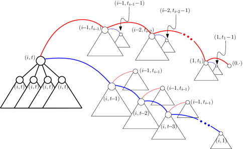
Figure 7: Schematic diagram of the $O^{*}(n)$-size data structure $\Psi_{v}^{(i,t)}$, constructed on a $(i,t)$-level node $v$. Red and blue threads illustrate recursion on $i$ and $t$, respectively.

Query procedure.

Let $Q\in\mathscr{Q}$ be a query object. Roughly speaking, for each $i\in[0,k]$, using $\Psi$, we compute the subset

$$\Phi_{\Pi}^{(i)}(Q)\coloneqq\{O\in\mathscr{O}\mid\bigwedge_{j=i+1}^{k}\left(g_{j}(O^{*},Q^{*})\geq 0\right)\},$$

the output of $\Pi_{i}$-query on $Q$, as the union of a small number of canonical subsets $\O_{1},\ldots,\O_{u}$, associated with respective $(i,\cdot)$-level nodes $v_{1},\ldots,v_{u}$ of $\Psi$. For $i=0$, $\Phi_{\Pi}^{(0)}(Q)=\Phi_{\Pi}(Q)$, so these canonical subsets form the output of the $\Pi$-query for $Q$, and we simply add their prestored weights (in the corresponding semigroup). For $i\geq 1$, for each $j\leq u$, we recursively search in the secondary structure $\Psi^{(i-1,t_{i-1})}_{v_{j}}$ for answering the extended $\Pi_{i-1}$-query on $\mathscr{C}_{j}$ with $Q$.

In more detail, we traverse $\Psi$ in a top-down manner, and maintain a partial sum $\mu$. Initially, $\mu=0$ and we start at the root of $\Psi$. Suppose we are at a node $v$ of an $(i,t)$-level tree. If $i=0$, we simply add $w_{v}=w(\mathscr{O}_{v})$ to $\mu$. So assume $i\geq 1$. If $v$ is a leaf of the tree, we scan the set $\mathscr{O}_{v}$ and add to $\mu$ the weights of those objects $O\in\mathscr{O}_{v}$ for which $\Pi_{i}(O,Q)=1$. If $v$ is an internal node, three cases can arise. Let $\widetilde{Q}_{i}=\{\mathbf{x}_{i}\in\mathbb{O}_{i}\mid g_{i}(\mathbf{x}_{i},Q_{i}^{*})\geq 0\}$ be the semi-algebraic region defined above. If $\tau_{v}\cap\widetilde{Q}_{i}=\emptyset$, we do not continue the processing at $v$. If $\tau_{v}\subseteq\widetilde{Q}_{i}$, we recursively search in the secondary structure $\Psi_{v}^{(i-1,t_{i-1})}$ with $Q$. Finally, if $\partial\widetilde{Q}^{(i)}\cap\tau_{v}\neq\emptyset$, which is equivalent to $Z(g_{i})\cap\tau_{i}\neq\emptyset$, we first recursively visit the secondary structure $\Psi_{v}^{(i,t-1)}$ (to search in the set $\mathscr{O}_{v}^{0}$), and then recursively search at every child of $v$.

$\Phi_{\Pi}(Q)$ can be represented as the union of the canonical subsets associated with the level-$0$ nodes that are visited by the query procedure, i.e., the nodes whose weights are added to produce $\mu$. The same query procedure can also represent $\neg{\Phi}_{\Pi}(Q)=\{O\in\mathscr{O}\mid\Pi(O,Q)=0\}$ as the union of few canonical subsets.

Analysis.

We now analyze the size and the query time of $\Psi$. For a node $v$ at some $(i,t)$-level, let $S(n_{v},i,t)$ be the maximum size of the partition tree constructed on at most $n_{v}$ objects with these parameters. We note that $S(n_{v},0,t)=O(1)$ and that for $n_{v}\leq n_{0}$ and $i\geq 1$ we have $S(n_{v},i,t)=O(n_{v})=O(1)$ too. For $t=1$, the corresponding tree is a balanced binary tree, so $S(n_{v},i,1)$ satisfies the following recurrence (for $n_{v}>n_{0}(i,1)$):

$$S(n_{v},i,1)\leq 2S(n_{v}/2,i,1)+S(n_{v},i-1,t_{i-1}).$$ (23)

Since $S(n_{v},i,t)=\Omega(n_{v})$ (since $S(n_{v},i,t)$ grows faster than a linear function), the solution of the above recurrence is

$$S(n_{v},i,1)=O(\log n_{v})\cdot S(n_{v},i-1,t_{i-1}).$$

Finally, for $t>1$ and $n_{v}>n_{0}$, we store at $v$ two secondary structures of levels $(i,t-1)$ and $(i-1,t_{i-1})$, and we recursively construct an $(i,t)$-level subtree on a set of at most $n_{v}/D$ objects for each of the $O(D)$ children of $v$. Hence, in this case, the recurrence is

$$S(n_{v},i,t)\leq c_{1}DS(n_{v}/D,i,t)+S(n_{v},i-1,t_{i-1})+S(n_{v},i,t-1),$$ (24)

where $t_{i-1}=\dim\left(\mathbb{O}_{i-1}\right)$ and $c_{1}\coloneqq c_{1}(i,t)$ is a constant. Using induction, it easily follows that, for any arbitrarily small constant $\varepsilon>0$, there exists a constant $A\coloneqq A(i,t,\varepsilon)$ such that the solution of the above recurrence is

$$S(n_{v},i,t)\leq An_{v}^{1+\varepsilon}.$$

That is, $S(n_{v},i,t)=O^{*}(n_{v})$ for each $i$ and $t$, where the constant of proportionality also depends on $i$ and $t$. Next, let $Q(n_{v},i,t)$ be the maximum time spent by a query at a node $v$ of some $(i,t)$-level that stores $n_{v}$ objects. We have $Q(n_{v},0,t)=O(1)$, and $Q(n_{v},i,t)=O(n_{v})$ for $n_{v}\leq n_{0}(i,t)$. For $t=1$, the analysis for a one-dimensional range tree implies that the query procedure visits nodes along $O(1)$ paths of the tree and the subproblem size at a node is at most half of that of its parent. Since $Q(n_{v},i,t_{i})=\Omega(n^{\varepsilon})$, for some constant $\varepsilon>0$, we obtain

$$Q(n_{v},i,1)=O(1)\cdot Q(n_{v},i-1,t_{i-1}).$$

Finally, consider $i\geq 1$, $t>1$ and $n_{v}>n_{0}(i,t)$. Since the degree of the partitioning polynomial is $O(D^{1/t})$ and the degree of $g_{i}$ is constant, $Z(g_{i})$ intersects $O(D^{1-1/t})$ cells of $Z(\mathscr{F})\setminus Z(F_{v})$ [19], which leads to the following recurrence:

$$Q(n_{v},i,t)\leq c_{2}D^{1-1/t}Q(n_{v}/D,i,t)+Q(n_{v},i-1,t_{i-1})+Q(n_{v},i,t-1),$$ (25)

where $c_{2}\coloneqq c_{2}(i,t)$ is a constant. The first term in the above recurrence follows from [40], and the second and third terms correspond to the query procedure visiting the secondary structures stored at $v$. Again, it can easily be shown that, for any arbitrarily small constant $\varepsilon>0$, there exists a constant $B\coloneqq B(i,t,\varepsilon)$ such that the solution of the above recurrence is

$$Q(n_{v},i,t)\leq Bn_{v}^{1-1/{t_{o}}+\varepsilon},\qquad\text{where}\quad{t_{o}}=\max_{1\leq i\leq k}t_{i}.$$

That is, $Q(n_{v},i,t)=O^{*}(n_{v}^{1-1/{t_{o}}})$ for each $i$ and $t$, where the constant of proportionality depends on $i$ and $t$. The same analysis implies that the subset of input objects that satisfy the query predicate can be represented as the union of $O^{*}(n_{v}^{1-1/{t_{o}}})$ canonical subsets.

Finally, as mentioned above, the data structure can be adapted to handle disjunctions for general aggregation queries such as counting queries. More precisely, suppose, for concreteness, that $\Pi(\mathbf{x},\mathbf{y})=\Pi_{1}(\mathbf{x},\mathbf{y})\vee\Pi_{2}(\mathbf{x},\mathbf{y})$, where each $\Pi_{i}$ is composed of only conjunctions. Set $\Pi^{\prime}_{2}(\mathbf{x},\mathbf{y})=(\neg\Pi_{1}(\mathbf{x},\mathbf{y}))\wedge\Pi_{2}(\mathbf{x},\mathbf{y})$. We first build a multi-level data structure $\Psi_{1}$ for $\Pi_{1}$. At each level-$0$ node $v$ of $\Psi_{1}$, we construct a data structure $\Psi_{2}$ for $\Pi^{\prime}_{2}$ on the corresponding subset of input objects. To answer a $\Pi$-query, we first compute $\mu_{1}$, the sum of weights of objects in $\Phi_{\Pi_{1}}(Q)$. Recall that $\Phi_{\neg\Pi_{1}}(Q)$ can also be represented as the union of canonical subsets associated with a few nodes of $\Psi_{1}$, namely, the $(i,\cdot)$-level internal nodes $v$ visited by the query procedure for which $\tau_{v}\cap\widetilde{Q}_{i}=\emptyset$. For every such node $v$, we query $\Psi_{2}^{v}$ with $Q$ and compute the weight of $\Phi_{\Pi_{2}}(Q)$. (We handle the leaf nodes visited by the query procedure separately.) The sum of the weights over all canonical subsets, denoted by $\mu_{2}$, returns the weight of $\Phi_{\Pi^{\prime}_{2}}(Q)$. We return $\mu_{1}+\mu_{2}$. It is easily seen that no object is included multiple times in the sum.

We thus have the following result.

Lemma A.3.

Let $\mathscr{O}$ be a set of $n$ geometric objects of constant complexity with reduced parametric dimension ${t_{o}}$, and let $\mathscr{Q}$ be a family of query objects of constant complexity. Let $\Pi\colon\mathscr{O}\times\mathscr{Q}\rightarrow\{0,1\}$ be a semi-algebraic predicate of constant complexity. $\mathscr{O}$ can be preprocessed, in $O^{*}(n)$ randomized expected time, into a data structure of size $O^{*}(n)$, so that a $\Pi$-query on $\mathscr{O}$ (with respect to any semigroup $\Sigma$) with an object in $\mathscr{Q}$ can be answered in $O^{*}(n^{1-1/{t_{o}}})$ time. The subset of input objects that satisfy the query predicate can be represented as the union of $O^{*}(n^{1-1/{t_{o}}})$ canonical subsets.

A.2 Space/query-time trade-off

Next, we show how the query time can be improved by increasing the size of the data structure. We now define $t_{i}=\dim(\mathbb{Q}_{i})$ and set ${t_{q}}\coloneqq\max_{1\leq i\leq k}t_{i}$. That is, ${t_{q}}$ is the reduced parametric dimension of $\mathscr{Q}$ with respect to $\Pi$. Let $s\in[n,n^{{t_{q}}}]$ be a given so-called storage parameter; the data structure we build will have size (and expected preprocessng cost) $O^{*}(s)$.

Data structure.

We now work in the query space $\mathbb{Q}$ and construct a multi-level partition tree $\varUpsilon$ on $\widetilde{\mathscr{O}}\coloneqq\{\widetilde{O}\mid O\in\mathscr{O}\}$ for answering point-enclosure queries with a query point $Q^{*}\in\mathbb{Q}$, using Lemma A.2. When the size of a subproblem falls below some threshold (now in general not a constant), we switch to the object space and build a data structure on the current canonical set of objects using Lemma A.3. If we set the threshold to a constant and simply store the $O(1)$ objects at each leaf, we obtain a data structure of size $O^{*}(n^{{t_{q}}})$ with $O^{*}(1)$ query time, see below. Our structure interpolates between these two extreme performance bounds, the one just mentioned and the one in Lemma A.3.

At each recursive step, we are at a node $v$ of $\varUpsilon$, and we construct an $(i,t)$-level partition tree $\varUpsilon^{(i,t)}$, for $0\leq i\leq k$ and $1\leq t\leq t_{i}$, for answering $\Pi_{i}$-queries on some canonical subset $\mathscr{O}_{v}\subseteq\mathscr{O}$ with a query object $Q$, such that $Q_{i}^{*}$ lies on some given $t$-dimensional variety of constant complexity. More precisely, we now have a $4$-tuple $(\mathscr{O}_{v},s_{v},\mathscr{F},i)$ where $\mathscr{F}$ is a set of $O(1)$ constant-degree polynomials in $\mathbb{R}[\mathbf{y}_{i}]$, $\mathscr{O}_{v}\subseteq\mathscr{O}$ is a canonical set associated with $v$, and $s_{v}$ is a storage parameter. We wish to construct a data structure of size $O^{*}(s_{v})$ on $\mathscr{O}_{v}$, in expected $O^{*}(s_{v})$ preprocessing time, for answering efficiently $\Pi_{i}$-queries on $\mathscr{O}_{v}$ with a query object $Q$ such that $Q_{i}^{*}\in Z(\mathscr{F})$; see below for the analysis of the efficiency of the query. As before, $v$ is associated with a semi-algebraic cell $\tau_{v}\subset Z(\mathscr{F})$, obtained from a suitable polynomial partitioning. Initially, $\mathscr{O}_{v}=\mathscr{O}$, $s_{v}=s$, $\mathscr{F}=\emptyset$, $i=k$, and $\tau_{v}=\mathbb{Q}^{(i)}$.

For $i=0$, $\varUpsilon^{(0,t)}$ is a singleton node that stores $w(\mathscr{O}_{v})$. So assume $i\geq 1$.

If $t=1$, $Z(\mathscr{F})$ is a one-dimensional curve, and we consider query objects $Q$ for which $Q_{i}^{*}$ lies on $Z(\mathscr{F})$. As before, it suffices to consider situations in which $Z(\mathscr{F})$ is connected. For an object $O\in\mathscr{O}$, let $\widetilde{O}\sqcap Z(\mathscr{F})$ denote the set of connected components (arcs) of $\widetilde{O}\cap Z(\mathscr{F})$. We compute $\mathscr{I}_{v}\coloneqq\bigcup\{\widetilde{O}_{i}\sqcap Z(\mathscr{F})\mid O\in\mathscr{O}_{v}\}$, which is a set of $O(|\mathscr{O}_{v}|)$ arcs on $Z(\mathscr{F})$, and build a segment tree $\varUpsilon_{v}^{(i,1)}$ on $\mathscr{I}_{v}$ [25]. Each node $z$ of $\varUpsilon_{v}^{(i,1)}$ is associated with an arc $\tau_{z}\subseteq Z(\mathscr{F})$, a subset $\mathscr{O}_{z}\subseteq\mathscr{O}_{v}$ of objects $O$ for which an endpoint of $\widetilde{O}_{i}\cap Z(\mathscr{F})$ lies in $\tau_{z}$, and another subset $\mathscr{C}_{z}\subseteq\mathscr{O}_{v}$, such that, for each $\widetilde{O}\in\mathscr{C}_{z}$ we have $\tau_{z}\subseteq\widetilde{O}_{i}$ but $\tau_{p(z)}\not\subset\widetilde{O}_{i}\cap Z(\mathscr{F})$ (where $p(z)$ is the parent of $z$). If $z$ is a node of depth $\delta$ in the segment tree $\varUpsilon_{v}^{(i,1)}$, we construct an $(i-1,t_{i-1})$-level structure $\varUpsilon_{z}^{(i-1,t_{i-1})}$ on $\mathscr{C}_{z}$ with space parameter $s_{v}/2^{\delta}$, i.e., for the subproblem $(\mathscr{C}_{z},s_{v}/2^{\delta},\emptyset,i-1)$, and attach $\varUpsilon_{z}^{(i-1,t_{i-1})}$ to $z$ as its secondary structure.

Finally, assume that $i\geq 1$ and $t>1$. We fix a threshold parameter $n_{0}\coloneqq(n^{t}/s)^{\tfrac{1}{t-1}}$. If $n_{v}\leq n_{0}$, $v$ is a leaf of $\varUpsilon$, and we construct a data structure $\Psi_{v}$ of size $O^{*}(n_{v})$, as described in Section A.1, for the subproblem $(\mathscr{O}_{v},\emptyset,i)$, using Lemma A.3 (the storage parameter is irrelevant in this case). So assume that $n_{v}>n_{0}$. Set $\widetilde{\mathscr{O}}_{v,i}\coloneqq\{\widetilde{O}_{i}\subseteq\mathbb{Q}_{i}\mid O\in\mathscr{O}_{v}\}$ to be a family of semi-algebraic sets in $\mathbb{Q}_{i}$. We choose a sufficiently large constant $D\coloneqq D(i,t)$, and compute a partitioning polynomial $F_{v}$ for $\widetilde{\mathscr{O}}_{v,i}$ with respect to $Z(\mathscr{F})$, using Lemma A.2 and the notations therein. Taking $D$ to be sufficiently large, we write the degree of $F_{v}$ as $O(D)$, and the number of cells into which it partitions $Z(\mathscr{F})$ as $O(D^{t})$, where each cell is crossed by at most $n_{v}/D$ regions. We recursively construct an $(i,t-1)$-level data structure $\varUpsilon^{(i,t-1)}_{v}$ for the subproblem $(\mathscr{O}_{v},s_{v},\mathscr{F}\cup\{F_{v}\},i)$ and attach it to $v$ as one of its secondary structures. For each cell $\tau$ of $Z(\mathscr{F})\setminus Z(F_{v})$, we create a child $z_{\tau}$ of $v$. We construct a semi-algebraic representation of $\tau$ and store it at $z_{\tau}$. Set $\mathscr{O}_{\tau}=\{O\in\mathscr{O}_{v}\mid\partial\widetilde{O}_{i}\cap\tau\neq\emptyset\}$, and $\mathscr{C}_{\tau}=\{O\in\mathscr{O}_{v}\mid\tau\subseteq\widetilde{O}_{i}\}$. We construct an $(i-1,t_{i-1})$-level data structure $\varUpsilon_{\tau}^{(i-1,t_{i-1})}$ on $\mathscr{C}_{\tau}$ and store it as a secondary structure at the child $z_{\tau}$. Finally, we recursively construct from $z_{\tau}$ an $(i,t)$-level subtree $\varUpsilon_{\tau}^{i,t}$ for the subproblem $(\mathscr{O}_{\tau},s_{v}/D^{t},\mathscr{F},i)$. As for the linear-size data structure, stores two secondary structures are attached to each node $v$—an $(i,t-1)$-level data structure on $\mathscr{O}_{v}^{0}$ and an $(i-1,t_{i-1})$-level data structure on the subset of objects $O\in\mathscr{O}_{p(v)}$ for which $\tau_{v}\subseteq\widetilde{O}_{i}$. This completes the description of the data structure.

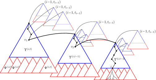
Figure 8: Shcematic diagram of $\varUpsilon^{(i,t)}$. The query procedure visits a path in level $(i,\cdot)$ trees (shown in black), recursively visits nodes in $(i-1,\cdot)$-level secondary structures attached to each node on the path, and eventually visits a subtree of the small-size data structure $\Psi$ attached to a leaf (node $z$ in the figure).

Query procedure.

Let $Q\in\mathscr{Q}$ be a query object. The basic idea is the same as above: we compute the query output as the aggregate weight of the union of a set of canonical subsets at the nodes that the query reaches. Since we allow more storage, the number of canonical subsets needed to compose the query output becomes smaller.

In more detail, we traverse $\varUpsilon$ in a top-down manner, and maintain a partial sum $\mu$. Initially, $\mu=0$ and we start at the root of $\varUpsilon$. Suppose we are at a node $v$ of an $(i,t)$-level tree $\varUpsilon_{v}^{(i,t)}$, such that $Q_{i}^{*}\in\tau_{v}$. If $i=0$, we add the weight $w_{v}=w(\mathscr{O}_{v})$ to $\mu$ and return. So assume $i\geq 1$.

We recursively query the $(i-1,t_{i-1})$-level secondary structure $\varUpsilon^{(i-1,t_{i-1})}$ with $Q$ and add the resulting weight to $\mu$. Next, if $v$ is a leaf, we query the structure $\Psi_{v}$ stored at $v$, using Lemma A.3, and add the resulting aggregate weight to $\mu$. Finally, assume that $v$ is an internal node. If $t=1$, we check which of the two intervals associated with the children of $v$ contains $Q_{i}^{*}$, and recursively search there. If $t>1$, we check whether the point $Q_{i}^{*}$ lies on $Z(F_{v})$. If the answer is yes, we recursively search with $Q$ in the $(i,t-1)$-level structure $\varUpsilon^{(i,t-1)}$ stored at $v$. Otherwise we find the child $z$ of $v$ such that $Q_{i}^{*}\in\tau_{z}$, and recursively search at $z$. Adding to $\mu$ the weights resulting from each recursive call, we obtain the aggregate output of the query.

Analysis.

We now analyze the size and the query time of $\varUpsilon$. For a node $v$ at some $(i,t)$-level, let $S(n_{v},s_{v},i,t)$ be the maximum size of the partition tree constructed at $v$ (i.e., on a set of at most $n_{v}$ objects and with storage parameter $s_{v}$). We note that $S(n_{v},s_{v},0,t)=O(1)$. For $t=1$, the structure is a segment tree, which is basically a balanced binary tree and each object is stored at $O(\log n_{v})$ nodes, so it is easily seen that

$$S(n_{v},s_{v},i,1)=O(\log n_{v})\cdot S(n_{v},s_{v},i-1,t_{i-1}).$$

Finally, for $i\geq 1,t>1,n_{v}>n_{0}$, we store two secondary structures of levels $(i,t-1)$ and $(i-1,t_{i-1})$, and we construct an $(i,t)$-level subtree on a set of at most $n_{v}/D$ objects for each child of $v$, leading to the following recurrence:

$$S(n_{v},s_{v},i,t)\leq c_{3}D^{t}\cdot S(n_{v}/D,s_{v}/D^{t},i,t)+S(n_{v},s_{v},i-1,t_{i-1})+S(n_{v},s_{v},i,t-1),$$ (26)

where $c_{3}\coloneqq c_{3}(i,t)$ is a constant. By induction on $n_{v},i,t$, we can show that for any arbitrarily small constant $\varepsilon>0$, the overall size of the data structure is $O_{\varepsilon}(sn^{\varepsilon})=O^{*}(s)$.

The analysis of the expected preprocessing cost is nearly identical, and yields the same bound $O^{*}(s)$.

Next, let $Q(n_{v},s_{v},i,t)$ denote the maximum query time (for at most $n_{v}$ objects and storage parameter $s_{v}$). As before, $Q(n_{v},s_{v},0,t)=O(1)$.

For $i\geq 1$ and $t=1$, the query procedure follows a single path in the segment tree until it reaches a leaf, so

$$Q(n_{v},s_{v},i,1)\leq\sum_{j=0}^{\log(n_{v}/n_{0})}Q(n_{v}/2^{j},s_{v}/2^{j},i-1,t_{i-1})+O^{*}(n_{0}^{1-1/{t_{o}}}).$$

Next, consider the case $i\geq 1$ and $t>1$. For $n_{v}\leq n_{0}$, by Lemma A.3, the query time is $O(n_{v}^{1-1/{t_{o}}+\varepsilon})$, so assume that $n_{v}>n_{0}$. Recall that the query procedure visits the $(i-1,t_{i-1})$-level secondary structure attached to $v$, and it either visits a child of $v$ or the $(i,t-1)$-level secondary structure attached to $v$, depending on whether the point $Q_{i}^{*}$ does not or does lie on $Z(F_{v})$. We thus obtain the following recurrence:

$$Q(n_{v},s_{v},i,t)\leq Q(n_{v},s_{v},i-1,t_{i-1})+\max\Bigl{\{}Q(n_{v}/D,s_{v}/D^{t},i,t),\,Q(n_{v},s_{v},i,t-1)\Bigr{\}}.$$ (27)

We claim that the overall query time is

$$Q(n_{v},s_{v},i,t)\leq c_{i}n_{0}^{1-1/{t_{o}}+\varepsilon}\log^{i-1}(n_{v}/n_{0})(\log(n_{v}/n_{0})+t),$$ (28)

for any $\varepsilon>0$ and a suitable sequence of constant coefficients $c_{i}$. For $n_{v}>n_{0}$, by induction on $n_{v},i$, and $t$, using (27), and using the fact that the query time is $O(n_{v}^{1-1/{t_{o}}+\varepsilon})$ for $n_{v}\leq n_{0}$, we obtain for $t>1$ (the case of $t=1$ is simpler)

$$Q(n_{v},s_{v},i,t) \leq c_{i-1}n_{0}^{1-1/{t_{o}}+\varepsilon}\log^{i-2}(n_{v}/n_{0})(\log(n_{v}/n_{0})+t_{i-1})$$

$$\quad+c_{i}n_{0}^{1-1/{t_{o}}+\varepsilon}\log^{i-1}(n_{v}/n_{0})\max\biggl{\{}\log\frac{n_{v}/D}{n_{0}}+t,\,\log\frac{n_{v}}{n_{0}}+t-1\biggr{\}}$$

$$\leq c_{i}n_{0}^{1-1/{t_{o}}+\varepsilon}\log^{i-1}(n_{v}/n_{0})\left(1+\max\biggl{\{}\log\frac{n_{v}/D}{n_{0}}+t,\,\log\frac{n_{v}}{n_{0}}+t-1\biggr{\}}\right)$$

(assming $$c_{i}\geq tc_{i-1}$$)

$$\leq c_{i}n_{0}^{1-1/{t_{o}}+\varepsilon}\log^{i-1}(n_{v}/n_{0})(\log(n_{v}/n_{0})+t).$$

Hence, the overall query time is

$$O^{*}(n_{0}^{1-1/{t_{o}}})=O^{*}\biggl{(}(n^{{t_{q}}}/s)^{\frac{1-1/{t_{o}}}{{t_{q}}-1}}\biggr{)}=O^{*}\biggl{(}(n/s^{1/{t_{q}}})^{\frac{1-1/{t_{o}}}{1-1/{t_{q}}}}\biggr{)}.$$

We thus have the main result of this appendix:

Theorem A.4.

Let $\mathscr{O}$ be a set of $n$ geometric objects of constant complexity, and let $\mathscr{Q}$ be a family of query objects of constant complexity. Let $\Pi\colon\mathscr{O}\times\mathscr{Q}\rightarrow\{0,1\}$ be a semi-algebraic predicate of constant complexity, and let ${t_{o}},{t_{q}}$ be the respective reduced parametric dimensions of $\mathscr{O}$ and $\mathscr{Q}$ with respect to $\Pi$. For a storage parameter $s\in[n,n^{{t_{q}}}]$, $\mathscr{O}$ can be preprocessed, in $O^{*}(s)$ expected time, into a data structure of size $O^{*}(s)$, so that a $\Pi$-query on $\mathscr{O}$ with an object $Q\in\mathscr{Q}$ can be answered in $O^{*}\biggl{(}(n/s^{1/{t_{q}}})^{\tfrac{1-1/{t_{o}}}{1-1/{t_{q}}}}\biggr{)}$ time.

If we perform $m$ $\Pi$-queries on $\mathscr{O}$ with the objects of $\mathscr{Q}$, for some $m>0$, then the total expected time spent, including the time to construct the data structure, is

$$O^{*}\biggl{(}s+m(n/s^{1/{t_{q}}})^{\tfrac{1-1/{t_{o}}}{1-1/{t_{q}}}}\biggr{)}.$$

By choosing the storage parameter

$$s=\min\left\{n^{t_{q}},\max\left\{n,m^{\tfrac{1-1/{t_{q}}}{1-1/{t_{o}}{t_{q}}}}n^{\tfrac{1-1/{t_{o}}}{1-1/{t_{o}}{t_{q}}}}\right\}\right\},$$

we obtain the following:

Corollary A.5.

Let $\mathscr{O}$ be a set of $n$ geometric objects of constant complexity, and let $\mathscr{Q}$ be a family of query objects of constant complexity. Let $\Pi\colon\mathscr{O}\times\mathscr{Q}\rightarrow\{0,1\}$ be a semi-algebraic predicate of constant complexity, and let ${t_{o}},{t_{q}}$ be the respective reduced parametric dimensions of $\mathscr{O}$ and $\mathscr{Q}$ with respect to $\Pi$. For any given $m>0$, $m$ $\Pi$-queries on $\mathscr{O}$ with the objects of $\mathscr{Q}$ can be performed in a total of

$$\biggl{(}m^{\tfrac{1-1/{t_{q}}}{1-1/{t_{o}}{t_{q}}}}n^{\tfrac{1-1/{t_{o}}}{1-1/{t_{o}}{t_{q}}}}+m+n\biggr{)}$$

expected time. For ${t_{o}}={t_{q}}=t$, the total expected time is

$$O^{*}\biggl{(}(mn)^{\tfrac{1}{1+1/t}}+m+n\biggr{)}.$$

Corollary A.5 can be used to compute a compact representation of the collection of pairs of objects that satisfy a semi-algebraic predicate: Let $\mathscr{A}$ and $\mathscr{B}$ be two sets of geometric objects, let $\Pi\colon\mathscr{A}\times\mathscr{B}\rightarrow\{0,1\}$ be a semi-algebraic predicate of constant complexity, and let $\mathscr{A}\Pi\mathscr{B}=\{(A,B)\mid\Pi(A,B)=1\}$ be the collection of pairs that satisfy the predicate. A biclique cover of $\mathscr{A}\Pi\mathscr{B}$ is a family $\mathscr{F}=\{(\mathscr{A}_{1},\mathscr{B}_{1}),\ldots,(\mathscr{A}_{r},\mathscr{B}_{r})\}$ such that (i) for any $1\leq i\leq r$ and for any $(A,B)\in\mathscr{A}_{i}\times\mathscr{B}_{i}$, $\Pi(A,B)=1$, and (ii) for any $(A,B)\in\mathscr{A}\times\mathscr{B}$ with $\Pi(A,B)=1$, there is a index (not necessarily unique) $j\leq r$ such that $(A,B)\in\mathscr{A}_{j}\times\mathscr{B}_{j}$. The size of the biclique cover $\mathscr{F}$ is $\sum_{i=1}^{r}\left(|\mathscr{A}_{i}|+|\mathscr{B}_{i}|\right)$. If every pair of $\mathscr{A}\Pi\mathscr{B}$ appears only once in $\mathscr{F}$, then we refer to $\mathscr{F}$ as a biclique partition of $\mathscr{A}\Pi\mathscr{B}$. A biclique cover of $\mathscr{A}\Pi\mathscr{B}$ can be computed as follows: We preprocess $\mathscr{A}$ into a data structure using Lemma A.3, and we query it with each object in $\mathscr{B}$. Let $\mathscr{A}_{1},\ldots,\mathscr{A}_{r}$ be the family of canonical subsets constructed by the data structure. By construction, the size of the data structure is proportional to $\sum_{i=1}|\mathscr{A}_{i}|$. For an object $B\in\mathscr{B}$, let $\mathscr{C}(B)$ be the subfamily of the canonical subsets that represent the set $\Phi_{\Pi}(B)$. For $1\leq i\leq r$, we set $\mathscr{B}_{i}\subseteq\mathscr{B}$ to be the subset of objects for which $\mathscr{A}_{i}$ is in $\mathscr{C}(B)$. Then $\{(\mathscr{A}_{i},\mathscr{B}_{i})\mid 1\leq i\leq r\}$ is the desired biclique cover, and $\sum_{i}|\mathscr{B}_{i}|=\sum_{B\in\mathscr{B}}|\mathscr{C}(B)|$. By Corollary A.5, we obtain the following:

Corollary A.6.

Let $\mathscr{A}$ and $\mathscr{B}$ be two sets of geometric objects of sizes $n$ and $m$, respectively, $\Pi\colon\mathscr{A}\times\mathscr{B}\rightarrow\{0,1\}$ a semi-algebraic predicate of constant complexity, and ${t_{a}},{t_{b}}$ the reduced parametric dimension of $\mathscr{A}$ and $\mathscr{B}$, respectively. Then a biclique cover of $\mathscr{A}\Pi\mathscr{B}$ of size $O^{*}\biggl{(}m^{\tfrac{1-1/{t_{b}}}{1-1/{t_{a}}{t_{b}}}}n^{\tfrac{1-1/{t_{a}}}{1-1/{t_{a}}{t_{b}}}}+m+n\biggr{)}$ can be computed in expected time $O^{*}\biggl{(}m^{\tfrac{1-1/{t_{b}}}{1-1/{t_{a}}{t_{b}}}}n^{\tfrac{1-1/{t_{a}}}{1-1/{t_{a}}{t_{b}}}}+m+n\biggr{)}$. For ${t_{a}}={t_{b}}=t$ and $m=n$, the bounds become $O^{*}(n^{\tfrac{2}{1+1/t}})$. If for any pair $(A,B)\in\mathscr{A}\Pi\mathscr{B}$ exactly one disjunct of $\Pi$ is $1$, then $\mathscr{F}$ is a biclique partition.

Special cases of Corollary A.6 have been used for a wide range of geometric optimization problems as well as for representing geometric graphs compactly [15, 39, 10]. For example, it implies that the edges in the intersection graph of a set of $n$ segments or unit disks (resp. disks of arbitrary radii) in the plane can be represented as a biclique cover of size $O^{*}(n^{4/3})$ (resp. $O^{*}(n^{3/2})$) as $t=2$ (resp. $t=3$) in these setups. The cover can be computed within the same time bound.

Remark 5.

(i) We note that the query time in the first data structure (cf. Lemma A.3) only depends on ${t_{o}}$ (and not on ${t_{q}}$). Therefore if multiple polynomial inequalities use the same subset of parameters of the input objects, we can combine these inequalities into a single predicate $\Pi_{i}^{O}(\mathbf{x}_{i},\mathbf{y})$. More generally, the first data structure can handle a predicate of the form

$$\Pi(\mathbf{x},\mathbf{y})=\bigwedge_{i=1}^{k}\Pi_{i}^{O}(\mathbf{x}_{i},\mathbf{y}),$$

where each $\Pi_{i}^{O}$ is an arbitrary semi-algebraic predicate of constant complexity (possibly containing disjunctions). Similarly, the top portion of the second data structure, which is constructed in the query space, can handle an equally general predicate of the form

$$\Pi(\mathbf{x},\mathbf{y})=\bigwedge_{i=1}^{k}\Pi_{i}^{Q}(\mathbf{x},\mathbf{y}_{i}),$$

by lumping together several subpredicates that use the same subset of the query parameters. We note that the compressed predicate could reduce the number of levels in the data structure, and that each sub-predicate could have disjunctions. Although this observation improves the performance of the data structure by only at most a polylogarithmic factor, it often simplifies the data structure considerably.

For example, suppose we wish to construct a linear-size data structure to perform planar double-wedge range queries, where the query objects are double wedges $W$, bounded by two lines $\ell_{1}$ and $\ell_{2}$, that do not contain the vertical line (the segment-intersection query for a set of lines in $\mathbb{R}^{2}$ can be formulated as double-wedge range query using the standard duality transform). Regarding $\ell_{1},\ell_{2}$ as linear functions, the intersection predicate in this case is

$$\Pi(\mathbf{x})=((\ell_{1}(\mathbf{x})\geq 0)\wedge(\ell_{2}(\mathbf{x})\leq 0))\vee((\ell_{1}(\mathbf{x})\leq 0)\wedge(\ell_{2}(\mathbf{x})\geq 0)).$$

Instead of constructing two separate two-level partition trees, we can construct a single one-level partition tree on the input points. The query procedure recursively visits the children of a node $v$ if the boundary $\partial W$ (i.e., one of the lines bounding $W$) intersects the cell $\tau_{v}$.

(ii) In either of the two data structures, when the size of a subproblem falls below the threshold $n_{0}$ (i.e., at a leaf), one could build a completely different data structure for answering queries on the subproblem (such as our construction of a data structure based on polynomial partitioning in $3$-space in Section 5). Similarly, one could replace the level-$1$ data structure with a different one that is more efficient. Such an approach sometimes leads to better query time for detection (emptiness) and reporting queries, as in the case of halfspace-emptiness queries. See, e.g., [43, 50].

References

- [1] S. S. Abhyankar and C. L. Bajaj. Automatic parameterization of rational curves and surfaces III: algebraic plane curves. Comput. Aided Geom. Des., 5(4):309–321, 1988.
- [2] S. S. Abhyankar and C. L. Bajaj. Automatic parameterization of rational curves and surfaces IV: algebraic space curves. ACM Trans. Graph., 8:325–334, 1989.
- [3] P. Afshani and P. Cheng. Lower bounds for semialgebraic range searching and stabbing problems. In Proc. 37th Intl. Sympos. Comput. Geom., pages 8:1–8:15, 2021.
- [4] P. Afshani and P. Cheng. On semialgebraic range reporting. In Proc. 38th Intl. Sympos. Comput. Geom., pages 3:1–3:14, 2022.
- [5] P. Afshani and P. Cheng. Lower bounds for intersection reporting among flat objects. In Proc. 39th Intl. Sympos. Comput. Geom., pages 3:1–3:16, 2023.
- [6] P. K. Agarwal. Ray shooting and other applications of spanning trees with low stabbing number. SIAM J. Comput., 21(3):540–570, 1992.
- [7] P. K. Agarwal. Simplex range searching and its variants: A review. In Journey through Discrete Mathematics: A Tribute to Jiří Matoušek, pages 1–30. Springer, Berlin, 2017.
- [8] P. K. Agarwal, B. Aronov, E. Ezra, and J. Zahl. An efficient algorithm for generalized polynomial partitioning and its applications. SIAM J. Comput., 50:760–787, 2021.
- [9] P. K. Agarwal, B. Aronov, and S. Suri. Stabbing triangulations by lines in 3D. In Proc. 11th Annu. Sympos. on Computational Geometry, pages 267–276, 1995.
- [10] P. K. Agarwal and J. Erickson. Geometric range searching and its relatives. In Advances in Discrete and Computational Geometry, volume 223 of Contemp. Math., pages 1–56. AMS Press, Providence, RI, 1999.
- [11] P. K. Agarwal and J. Matousek. On range searching with semialgebraic sets. Discrete Comput. Geom., 11:393–418, 1994.
- [12] P. K. Agarwal and J. Matoušek. Ray shooting and parameric search. SIAM J. Comput., 22:794–806, 1993.
- [13] P. K. Agarwal, J. Matoušek, and M. Sharir. On range searching with semialgebraic sets II. SIAM J. Comput., 42:2039–2062, 2013.
- [14] P. K. Agarwal and M. Sharir. Ray shooting amidst convex polyhedra and polyhedral terrains in three dimensions. SIAM J. Comput., 25(1):100–116, 1996.
- [15] P. K. Agarwal and K. R. Varadarajan. Efficient algorithms for approximating polygonal chains. Discrete Comput. Geom., 23(2):273–291, 2000.
- [16] B. Aronov, E. Ezra, and J. Zahl. Constructive polynomial partitioning for algebraic curves in with applications. SIAM J. Comput., 49:1109–1127, 2020.
- [17] B. Aronov and S. Fortune. Approximating minimum-weight triangulations in three dimensions. Discrete Comput. Geom., 21(4):527–549, 1999.
- [18] B. Aronov, E. Y. Miller, and M. Sharir. Eliminating depth cycles among triangles in three dimensions. Discrete Comput. Geom., 64(3):627–653, 2020.
- [19] S. Basu, R. Pollack, and M.-F. Roy. Algorithms in Real Algebraic Geometry. Springer, Berlin, 2003.
- [20] J. L. Bentley. Multidimensional divide-and-conquer. Commun. ACM, 23(4):214–229, 1980.
- [21] T. G. Berry. Parametrization of algebraic space curves. J. Pure Applied Algebra., 117:81–95, 1997.
- [22] B. Chazelle. Fast searching in a real algebraic manifold with applications to geometric complexity. In Proc. Intl. Joint Conf. Theory and Practice of Software Development, pages 145–156, 1985.
- [23] G. E. Collins. Quantifier elimination for the elementary theory of real closed fields by cylindrical algebraic decomposition. In Proc. 2nd GI Conf. Automata Theory and Formal Languages, pages 134–183, 1975.
- [24] D. Cox, J. Little, and D. O’Shea. Ideals, Varieties and Algorithms: An Introduction to Computational Algebraic Geometry and Commutative Algebra. Springer, Berlin, 2015.
- [25] M. de Berg, O. Cheong, M. J. van Kreveld, and M. H. Overmars. Computational Geometry: Algorithms and Applications, 3rd Edition. Springer, Berlin, 2008.
- [26] M. de Berg, D. Halperin, M. H. Overmars, J. Snoeyink, and M. J. van Kreveld. Efficient ray shooting and hidden surface removal. Algorithmica, 12(1):30–53, 1994.
- [27] D. P. Dobkin and H. Edelsbrunner. Space searching for intersecting objects. J. Algorithms, 8(3):348–361, 1987.
- [28] D. P. Dobkin and D. G. Kirkpatrick. Fast detection of polyhedral intersection. Theor. Comput. Sci., 27:241–253, 1983.
- [29] E. Ezra and M. Sharir. Intersection searching amid tetrahedra in 4-space and efficient continuous collision detection. In Proc. 30th Annual European Symposium on Algorithms, pages 51:1–51:17, 2022.
- [30] E. Ezra and M. Sharir. On ray shooting for triangles in 3-space and related problems. SIAM J. Comput., accepted.
- [31] A. Galligo and N. N. V. Jr. Complexity of finding irreducible components of a semialgebraic set. J. Complex., 11(1):174–193, 1995.
- [32] L. Guth. Polynomial partitioning for a set of varieties. Math. Proc. Camb. Phil. Soc., 159:459–469, 2015.
- [33] L. Guth. Ruled Surface Theory and Incidence Geometry, pages 449–466. Springer, Berlin, 2017.
- [34] L. Guth and N. H. Katz. On the Erdős distinct distances problem in the plane. Annals Math., 181:155–190, 2015.
- [35] J. Hershberger and S. Suri. A pedestrian approach to ray shooting: Shoot a ray, take a walk. J. Algorithms, 18(3):403–431, 1995.
- [36] E. Kaltofen. Polynomial factorization 1987–1991. In Proc. 1st Latin American Sympos. Theoretical Informatics, pages 294–313, 1992.
- [37] J. Matousek. Range searching with efficient hiearchical cutting. Discrete Comput. Geom., 10:157–182, 1993.
- [38] J. Matousek. Geometric range searching. ACM Comput. Surv., 26(4):421–461, 1994.
- [39] J. Matoušek. Randomized optimal algorithm for slope selection. Inf. Process. Lett., 39(4):183–187, 1991.
- [40] J. Matoušek and Z. Patáková. Multilevel polynomial partitions and simplified range searching. Discrete Comput. Geom., 54:22–41, 2015.
- [41] J. Maurer. Puiseux expansion for space curves. Manuscripta Mathematica, 32:91–100, 1980.
- [42] J. Milnor. Morse Theory. Princeton University Press, Princeton, 1963.
- [43] S. Mohaban and M. Sharir. Ray shooting amidst spheres in 3 dimensions and related problems. SIAM J. Comput., 26:654–674, 1997.
- [44] M. Pellegrini. Ray shooting on triangles in 3-space. Algorithmica, 9:471–494, 1993.
- [45] M. Pellegrini. Ray shooting and lines in space. In J. E. Goodman, J. O’Rourke, and C. D. Tóth, editors, Handbook on Discrete and Computational Geometry, pages 1093–1112. CRC Press, Boca Raton, Florida, 3rd edition, 2017.
- [46] S. Pérez-Díaz, J. R. Sendra, S. L. Rueda, and J. Sendra. Approximate parametrization of plane algebraic curves by linear systems of curves. Comput. Aided Geom. Des., 27(2):212–231, 2010.
- [47] F. P. Preparata and M. I. Shamos. Computational Geometry: An Introduction. Springer, Berlin, 1985.
- [48] J. T. Schwartz and M. Sharir. On the piano movers’ problem: II. General techniques for computing topological properties of real algebraic manifolds. Advances in Appl. Math., 4:298–351, 1983.
- [49] J. R. Sendra and D. Sevilla. Radical parametrizations of algebraic curves by adjoint curves. J. Symb. Comput., 46(9):1030–1038, 2011.
- [50] M. Sharir and H. Shaul. Ray shooting and stone throwing with near-linear storage. Comput. Geom. Theory Appls., 30:239–252, 2005.
- [51] R. J. Walker. Algebraic Curves. Dover Books, New York, 1962.
- [52] A. C. Yao and F. F. Yao. A general approach to d-dimensional geometric queries. In Proc. 17th Annu. ACM Symp. Theory of Computing, pages 163–168, 1985.