SDOAnet: An Efficient Deep Learning-Based DOA Estimation Network for Imperfect Array

Abstract

Direction of arrival (DOA) estimation is a fundamental problem in conventional radar and wireless communication applications and emerging integrated sensing and communication (ISAC) systems. Due to many imperfect factors in the low-cost systems, including the antenna position perturbations, the inconsistent gains/phases, the mutual coupling effect, the nonlinear amplifier effect, etc., the performance of the DOA estimation often degrades significantly. To characterize the realistic array more accurately, a novel deep learning (DL)-based DOA estimation method named super-resolution DOA network (SDOAnet) is proposed in this paper. Unlike the existing DL-based DOA methods, our proposed SDOAnet employs the sampled received signals, instead of the covariance matrices of the received signals, as the input of the convolution layers for extracting data features. Moreover, the output of SDOAnet is a vector independent of the DOA of targets but can be used to estimate their spatial spectrum. As a result, the same training network can be applied to any number of targets, significantly reducing the implementation complexity. At last, the convergence speed of our SDOAnet with a low-dimension network structure is much faster than existing DL-based methods. Simulation results show that the proposed SDOAnet outperforms the existing DOA estimation methods due to the imperfect array. The code about the SDOAnet is available online https://github.com/chenpengseu/SDOAnet.git.

I Introduction

Direction of arrival (DOA) estimation is a fundamental problem in the wireless communications, radar-based applications, and the future integrated sensing and communication (ISAC) systems [1, 2], and has been studied for decades. Typically, the DOA estimation is based on an ideal antenna array model, without considering any imperfect effect, including the mutual coupling effect, inconsistent gains/phases, nonlinear effect, etc. In this ideal scenario, the DOAs can be estimated by traditional methods such as the monopulse angle estimation method [3] and the fast Fourier transformation (FFT)-based methods.

Moreover, super-resolution estimation methods have also been proposed. On the one hand, subspace-based methods such as the algorithms of multiple-signal classification (MUSIC) [4, 5, 6] and estimation of signal parameters via rotational invariance techniques (ESPRIT) [7, 8, 9, 10] were proposed. On the other hand, sparse reconstruction-based methods have also been proposed by exploiting the signals’ sparsity in the spatial domain. For example, the compressed sensing (CS)-based methods for the DOA estimation have been proposed, such as sparse Bayesian learning-based methods [11, 12, 13, 14, 15, 16], the mixed $\ell_{2,0}$ norm-based methods [17], etc.

However, the above works did not consider the effect of imperfect antenna arrays. As a result, the performance of these algorithms is significantly affected in practical DOA estimation systems. In the literature, some works have started to investigate the DOA estimation schemes under imperfect antenna arrays. For example, for an array with mutual coupling, gain or phase errors, and sensor location errors, a method estimating DOA and model errors is proposed in [18]. A fourth-order parallel factor decomposition model using imperfect waveforms is given in [19] to estimate the DOA. Then, ref. [20] proposes a two-dimensional (2D) DOA estimation method for an imperfect L-shaped array using active calibration. However, each of the above works only considered a subset of the imperfect array effects, because optimization over the complicated array model with all imperfect effects considered is challenging. This motivates us to use the deep learning (DL) technique for DOA estimation with all imperfect array effects taken into account because of its efficiency for training over difficult networks.

In the literature, several works have been done for DL-based DOA estimation [21, 22, 23, 24], and have the advantages of low computational complexity and high accuracy. There are some types of DL-based methods:

1. The input data is the raw sampled data from the array;

2. The input data is the covariance matrix of the received signal;

3. The outputs are the directly estimated DOAs;

4. The output is the spatial spectrum and the DOAs are estimated from the spectrum.

For example, in [25, 26], a DL-based method is proposed for the DOA estimation, where the input is the covariance matrix and the output is the spectrum. A sparse loss function is used to train the network. Ref. [27] gives a CNN-based method for the DOA estimation using the estimated covariance matrix and estimates the DOA by discretizing the spatial domain into grids. In [28], a synthetic dataset for angle classification is shown under the presence of additive noise, propagation attenuation, and delay. Then, a CNN-based method is proposed for the DOA estimation. An angle separation learning method is proposed in [26] for the DOA estimation of the coherent signals, where the covariance matrix is formulated as the input features of the deep neural network (DNN). In [29], a deep convolution network (DCN) is given for the DOA estimation with the covariance matrix as the under-sampled linear measurements of the spatial spectrum, where the signal sparsity in the spatial domain is also exploited to improve the estimation performance. A MUSIC-based DOA estimation method is proposed in [30] by using small antenna arrays, where DL is formulated to reconstruct the signals of a virtual large antenna array. Ref. [22] gives an offline and online DNN method for the DOA estimation in the massive multiple-input multiple-output (MIMO) system, where DOA is the network output and can be estimated directly from the received signal. For the DOA estimation with a low signal-to-noise ratio (SNR), a convolutional neural network (CNN) is proposed in [31], where the covariance matrix is the network’s input and shows enhanced robustness in the presence of noise. Moreover, a multiple deep CNN is designed in [32], where each CNN learns the MUSIC spectrum of the received signal, so a nonlinear relationship between the received sensor data and the angular spectrum is formulated in the network. For the imperfect array, ref. [33] introduces a framework of the DNN to estimate the DOA using a multitask autoencoder and series of parallel multilayer classifiers.

We can find that the DL-based DOA estimation methods mainly use the CNN as a typical network structure [34], and the input is the statistic results such as the covariance matrix. Since the information in the statistical data limits the estimation performance, the performance cannot be better than that using the raw sampled data. Furthermore, the network output is the estimated DOAs, and the spatial spectrum cannot be obtained. Therefore, the network structure should be adjusted with different target numbers, and it is not suitable for practical applications. There are some limitations to the existing DL-based methods:

• Since the classic DOA estimation algorithms such as MUSIC is just based on the covariance matrices of the received signals, most existing ML-based schemes use these covariance matrices as the input data to train the network. However, the covariance matrices are not sufficient for the optimal estimator design in general. As a result, the input data used in these works does not preserve all the useful information.

• In addition, the output of the existing ML-based DOA estimation schemes is usually the spatial spectrum of the targets. In this case, the training network depends on the number of targets, i.e., different networks should be trained given a different number of targets. This is of high complexity in practice.

• Furthermore, when the spatial spectrum is used, we must discretize the DOAs into grids, and the possible DOA must be on the discretized grids exactly. More girds as the output must be used for high accuracy, and the network will become more complex and hard to train.

In this paper, we propose a new type of DNN network based on CNN, i.e., super-resolution DOA network (SDOAnet), to overcome the above-mentioned difficulties in the DOA estimation. The proposed SDOAnet is used for the performance evaluation of imperfect arrays under realistic conditions. Compared with the existing methods, the proposed SDOAnet can achieve better estimation performance with lower complexity. The contributions of this paper are given as follows:

1. A system model with imperfect array effects for the DOA estimation is formulated. The imperfect effect includes the position perturbation, the inconsistent gains, the inconsistent phases, the mutual coupling effect, and the nonlinear effect, etc. As a result, our results are directly applicable to a practical system.

2. A new DL architecture is proposed based on the imperfect array. Different from existing methods, the input of the SDOAnet is the raw sampled signals, and the output is a vector, which can be used to estimate the spatial spectrum easily. Convolution layers are then used to get the signals’ features and avoid the complexity of high-dimension signals. The output of the SDOAnet is a vector for the spectrum estimation and can avoid the problem of discretizing the spatial domain. Compared with the existing CNN-based method, the proposed SDOAnet can be trained easily and perform the better estimation.

3. A loss function to train the SDOAnet is proposed, where Gaussian functions are used to approximate the spatial spectrum. Inspired by the atomic norm minimization (ANM)-based DOA estimation method, the output of SDOAnet is used to formulate the spatial spectrum. Then, a loss function is used to measure the error between the refereed spectrum and the estimated one and to train the network.

The remainder of this paper is organized as follows. The system mode of practical DOA estimation is formulated in Section II. The review of the super-resolution DOA estimation method is given in Section III. Then, the proposed SDOAnet for the DOA estimation is shown in Section IV. Simulation results are carried out in Section V, and finally, Section VI concludes the paper.

Notations: Upper-case and lower-case boldface letters denote matrices and column vectors, respectively. The matrix transpose and the Hermitian transpose are denoted as $(\cdot)^{\text{T}}$ and $(\cdot)^{\text{H}}$, respectively. $\mathcal{R}\{\cdot\}$ and $\mathcal{I}\{\cdot\}$ denote the real and imaginary parts of a complex value, respectively. $\text{Tr}\{\cdot\}$ is the trace of a matrix. $\|\cdot\|_{2}$ is the $\ell_{2}$ norm.

II The System Model for Practical DOA Estimation

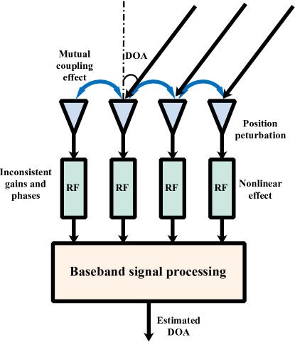
Figure 1: The system model for the DOA estimation in a practical array.

In this paper, we consider the DOA estimation problem in a practical system and propose a DL-based estimation framework. As shown in Fig. 1, we consider $K$ far-field signals, and the $k$-th ($k=0,1,\dots,K-1$) signal is expressed as $s_{k}(t)\in\mathbb{C}$ with the DOA being $\theta_{k}\in\left(-\frac{\pi}{2},\frac{\pi}{2}\right]$. A linear array system with $N$ antennas is used to receive the signals and estimate the DOAs, where the wavelength is denoted as $\lambda$. Considering an additive noise $w_{n}(t)\in\mathbb{C}$, the received signal at the $n$-th ($n=0,1,\dots,N-1$) antenna can be expressed as

$$r_{n}(t)=g\left(x_{n}(t)+\sum_{n^{\prime}\neq n}B_{n,n^{\prime}}x_{n^{\prime}}(t)\right)+w_{n}(t).$$ (1)

Then, we have

$$x_{n}(t)=\sum^{K-1}_{k=0}s_{k}(t)A_{n}e^{j\phi_{n}}e^{j2\pi\frac{d_{n}}{\lambda}\sin\theta_{k}},$$ (2)

where taking the $0$-th antenna as the reference one, i.e., $d_{0}=0$, the position of the $n$-th antenna is $d_{n}$, and for a uniform linear array (ULA), the position of the antenna is $d_{n}=n\lambda/2$. In the received signal (1), the following imperfect problems are considered:

1. The mutual coupling effect: The antennas cannot be ideally isolated and introduce the mutual coupling effect among the received signals. The mutual coupling coefficient between the $n$-th and $n^{\prime}$-th ($n\neq n^{\prime}$) antenna is $B_{n,n^{\prime}}\in\mathbb{C}$ with $|B_{n,n^{\prime}}|<1$ in (1);

2. The position perturbations: The antenna positions cannot be exactly at the desired positions, and will cause the phase errors of the received signals among antennas in the steering vector;

3. The inconsistent gains: The radio frequency (RF) channels usually cannot have exactly the same amplifiers, and will cause amplitude differences among the received signals. The channel gain of the $n$-th antenna is denoted as $A_{n}>0$;

4. The inconsistent phases: The difference among the RF channels will also cause the delay and phases errors of the received signals, and The channel phase of the $n$-th antenna is denoted as $\phi_{n}$;

5. The nonlinear effect: The nonlinear effect among RF channels and analog-to-digital converter (ADC) will introduce the nonlinear effect and degrade the DOA estimation performance. We use a nonlinear function $g(\cdot)$ to represent the nonlinear operation in the receiving channels.

Hence, collect the received signals into a vector

$$\boldsymbol{r}\triangleq\begin{bmatrix}r_{0}(t),r_{1}(t),\dots,r_{N-1}(t)\end{bmatrix}^{\text{T}}.$$ (3)

The DOA estimation problem can be formulated as a parameter estimation problem with the received signal $\boldsymbol{r}$. Most existing works consider the methods in the scenario with the perfect array, where we have the linear function $g(\cdot)$, the mutual coupling coefficient $B_{n,n^{\prime}}$ is $0$, the channel gains are the same ($A_{n}=1$ and $\phi_{0}=0$), and the position $d_{n}$ of the antenna is known.

However, when an imperfect array is considered, the imperfect elements include the mutual coupling effect, the nonlinear effect, the inconsistent phases, the inconsistent gains, and the position perturbations, etc. In the practical systems, most existing super-resolution methods cannot outperform the traditional methods, where the super-resolution methods must have perfect systems and high SNR. In this paper, we will focus on a robust super-resolution method for DOA estimation with imperfect system effects.

III The Review of Super-Resolution DOA Estimation Methods

III-A The Atomic Norm-Based Estimation Methods

In recent years, atomic norm-based methods have been proposed for line-spectra estimation and achieved better performance by exploiting the sparsity of the spectrum in the frequency domain. Additionally, the DOA estimation problem can be easily described as a line-spectral estimation problem, so atomic norm-based methods have been proposed for the DOA estimation.

Usually, in the atomic norm-based methods. the ideal ULA is assumed, and the received signal based on (1) in the $n$-th array can be expressed as

$$r_{n}=\sum^{K-1}_{k=0}s_{k}e^{j2\pi\frac{nd}{\lambda}\sin\theta_{k}}+w_{n}(t),$$ (4)

where the distance between adjacent antennas is $d=\frac{\lambda}{2}$. Then, with the definition of a steering vector

$$\boldsymbol{a}(\theta)\triangleq\begin{bmatrix}1,e^{j\frac{2\pi d}{\lambda}\sin\theta},\dots,1,e^{j\frac{2\pi(N-1)d}{\lambda}\sin\theta}\end{bmatrix}^{\text{T}},$$ (5)

collect all the received signals into a vector, and we have

$$\boldsymbol{r} \triangleq\begin{bmatrix}r_{0},r_{1},\dots,r_{N-1}\end{bmatrix}^{\text{T}}$$

$$=\boldsymbol{As}+\boldsymbol{w},$$ (6)

where we define the steering matrix as

$$\boldsymbol{A} \triangleq\begin{bmatrix}\boldsymbol{a}(\theta_{0}),\boldsymbol{a}(\theta_{1}),\dots,\boldsymbol{a}(\theta_{K-1})\end{bmatrix},$$ (7)

the signal vector is defined as

$$\boldsymbol{s} \triangleq\begin{bmatrix}s_{0},s_{1},\dots,s_{K-1}\end{bmatrix}^{\text{T}},$$ (8)

and the noise vector is

$$\boldsymbol{w} \triangleq\begin{bmatrix}w_{0},w_{1},\dots,w_{N-1}\end{bmatrix}^{\text{T}}.$$ (9)

In the ANM-based DOA estimation method, an atomic norm is defined as

$$\|\boldsymbol{x}\|_{\mathcal{A}}\triangleq\inf\Big{\{} \sum_{n}\alpha_{n^{\prime}}:\boldsymbol{x}=\sum\alpha_{n^{\prime}}e^{j\phi_{n^{\prime}}}\boldsymbol{a}(\theta_{n^{\prime}}),$$

$$\phi_{n^{\prime}}\in[0,2\pi),\alpha_{n^{\prime}}\geq 0\Big{\}},$$ (10)

which describes a sparse representation of $\boldsymbol{x}$ with the sparse coefficients being $\alpha_{n^{\prime}}$ ($n^{\prime}=0,1,\dots,N^{\prime}-1$). Then, with the received signal $\boldsymbol{r}$, we denoise the signal with a sparse reconstruction signal $\boldsymbol{x}$, which can be expressed as an ANM expression

$$\min_{\boldsymbol{x}}\frac{1}{2}\|\boldsymbol{r}-\boldsymbol{x}\|^{2}_{2}+\beta\|\boldsymbol{x}\|_{\mathcal{A}},$$ (11)

where the parameter $\beta$ is used to control the trade-off between the sparsity and the reconstruction accuracy. This ANM problem can be solved by introducing a semi-definite programming (SDP) method, which is

$$\min_{\boldsymbol{B},\boldsymbol{h}}\quad \|\boldsymbol{r}-\boldsymbol{h}\|^{2}_{2}$$

s.t $$\begin{bmatrix}\boldsymbol{B}&\boldsymbol{h}\\ \boldsymbol{h}^{\text{H}}&1\end{bmatrix}\succeq 0$$ (12)

$$\boldsymbol{B}\text{ is Hermitian matrix}$$

$$\text{Tr}\{\boldsymbol{B}\}=\beta^{2}$$

$$\sum_{n}\boldsymbol{B}_{n,n+n^{\prime}}=0,\text{ for }n^{\prime}\neq 0$$

$$\qquad\qquad\qquad\quad\text{ and }n^{\prime}=1-N,\dots,N-1.$$

By solving the SDP problem (III-A), the sparse reconstruction signal $\boldsymbol{h}$ can be obtained, and the DOA of the received signal can be estimated by finding the peak values of the following polynomial

$$f(\theta)=|\boldsymbol{a}^{\text{H}}(\theta)\boldsymbol{h}|^{2}.$$ (13)

The ANM-based DOA estimation method is for the ideal array with perfect assumptions, but for the practical array, the ANM-based method must be extended. In [35, 36, 37, 38], the atomic norm-based methods are extended for the practical array. We can find that the much complex optimization problems are formulated, and a vector like $\boldsymbol{h}$ denoted as $\boldsymbol{h}^{\prime}$ can be obtained. Then, the DOAs are estimated by the peak values of the following polynomial

$$f^{\prime}(\theta)=|\boldsymbol{a}^{\text{H}}(\theta)\boldsymbol{h}^{\prime}|^{2}.$$ (14)

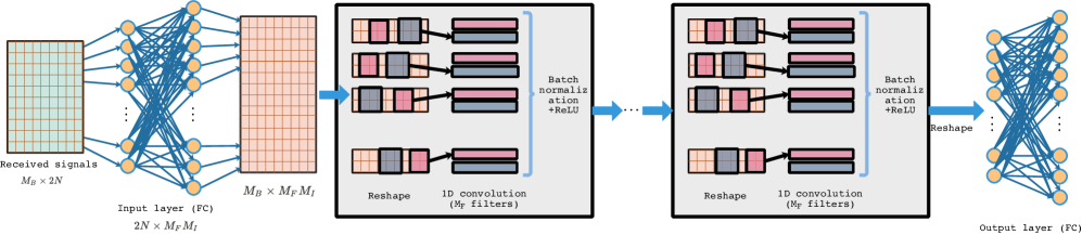
Figure 2: The network architecture of the proposed SDOAnet.

III-B The MUSIC-Based Estimated Methods

In the super-resolution estimation method, the MUSIC-based methods can perform better by using the noise and signal subspaces. For the single-snapshot spectral estimation, ref [39] proposes a MUSIC-based method. A Hankel matrix is obtained from the received signal $\boldsymbol{r}$ as

$$\boldsymbol{R}=\text{Hankel}(\boldsymbol{r})\begin{bmatrix}r_{0}&r_{1}&\dots&r_{N-L}\\ r_{1}&r_{2}&\dots&r_{N-L+1}\\ \vdots&\vdots&\ddots&\vdots\\ r_{L-1}&r_{L}&\dots&r_{N-1}\end{bmatrix},$$ (15)

where the received signal $\boldsymbol{r}$ is reshaped as a matrix $\boldsymbol{R}\in\mathbb{C}^{L\times N-L+1}$. Then, a singular value decomposition (SVD) is used as

$$[\boldsymbol{U}_{1},\boldsymbol{U}_{2}]\boldsymbol{\Lambda}[\boldsymbol{V}_{1},\boldsymbol{V}_{2}]=\text{SVD}\{\boldsymbol{R}\},$$ (16)

where $\boldsymbol{U}_{2}$ is corresponding to the small singular values and $\boldsymbol{\Lambda}$ is a diagonal matrix with the entries from the singular values. Finally, the spatial spectrum can be estimated as

$$g(\theta)=\frac{1}{\|\boldsymbol{a}^{\text{H}}(\theta)\boldsymbol{U}_{2}\|^{2}_{2}}.$$ (17)

IV The Proposed DOA Estimation Method

From the above sections about the existing DOA estimation methods, we can find that the DOAs are estimated by searching the peak values of the spatial spectrum. In this section, we will propose a new DL-based super-resolution method for DOA estimation, and it is named a super-resolution DOA network (SDOAnet), which contains more information and can be trained faster than the existing covariance matrix-based methods.

IV-A The SDOAnet Architecture

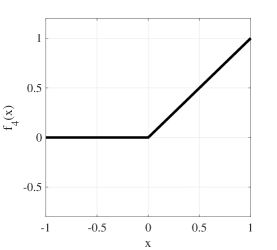
Figure 3: The ReLU function.

The SDOAnet architecture is shown in Fig. 2. First, the received signal in (1) is rewritten as a vector with real and imaginary parts

$$\boldsymbol{y}(t)\triangleq[\mathcal{R}^{\text{T}}\{\boldsymbol{r}(t)\},\mathcal{I}^{\text{T}}\{\boldsymbol{r}(t)\}]^{\text{T}}\in\mathbb{R}^{2N\times 1},$$ (18)

where we have the received signal vector

$$\boldsymbol{r}(t)=[r_{0}(t),r_{1}(t),\dots,r_{N-1}(t)]^{\text{T}}\in\mathbb{C}^{N\times 1}.$$ (19)

With the batch size being $M_{B}$, the input signal is

$$\boldsymbol{Y}\triangleq[\boldsymbol{y}(0),\boldsymbol{y}(1),\dots,\boldsymbol{y}(M_{B}-1)]^{\text{T}},$$ (20)

and the size is $M_{B}\times 2N$.

Then, since the SDOAnet is based on the convolution network, we use a full connection (FC) as the input layer with the output dimension being $M_{F}M_{I}$, where $M_{F}$ denotes the number of filters in the convolution layers and $M_{I}$ denotes the inner dimension extension. After the input layer, the dimension of the signal is $M_{B}\times M_{F}M_{I}$, and we reshape the signal as a tensor $f_{1}(\boldsymbol{Y})$ with the dimension being $M_{B}\times M_{F}\times M_{I}$, where $f_{1}(\cdot)$ is an input layer function.

The tensor is passed into the convolution layers and the number of convolution layers is $M_{C}$. In each convolution layer, a one-dimensional (1D) convolution operation is realized with the kernel size being $M_{F}\times M_{K}$ and the padding operation is used to keep that the size of the convolution output the same as that of input. The output of the convolution operation is $M_{B}\times M_{F}\times M_{I}$. Then, the batch normalization is applied to the convolution output, and the normalization output is denoted as $f_{3}(f_{2}(f_{1}(\boldsymbol{Y})))$. The function $f_{2}(\cdot)$ denotes the convolution operation and $f_{3}(\cdot)$ is the batch normalization operation

$$f_{3}(x)=\frac{x-\mathcal{E}\{x\}}{\sqrt{\text{Var}\{x\}+\epsilon}},$$ (21)

where $\mathcal{E}\{x\}$ and $\text{Var}\{x\}$ are the mean and variance of $x$, respectively. $\epsilon$ is a value added to the denominator for numerical stability and can be set as $\epsilon=10^{-5}$. In each convolution layer, a ReLU function $f_{4}(\cdot)$ as shown in Fig. 3 is applied on the output of the batch normalization and is defined as

$$f_{4}(x)\triangleq\max(0,x).$$ (22)

After the convolution layers, an FC layer is used as an output layer with the input and output sizes being $M_{B}\times M_{I}M_{F}$ and $M_{B}\times 2N$, respectively. The operation in the output layer is denoted as $f_{5}(\cdot)$.

Figure 4: The flowchart of the functional operations.

Finally, as shown in Fig. 4, we can obtain the output of the SDOAnet as

$$\boldsymbol{G}=f_{5}(f_{4}(f_{3}(f_{2}(f_{4}(\dots f_{4}(\dots f_{2}(f_{1}(\boldsymbol{Y}))\dots)\dots))))),$$ (23)

where we have

$$\boldsymbol{G}\triangleq\begin{bmatrix}\boldsymbol{g}(0),\boldsymbol{g}(1),\dots,\boldsymbol{g}(M_{B}-1)\end{bmatrix}\in\mathbb{R}^{M_{B}\times 2N}.$$ (24)

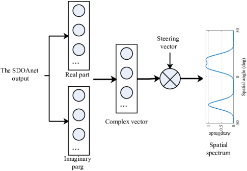
Figure 5: The flowchart to obtain the spatial spectrum from the network output.

As shown in Fig. 5, the corresponding complex vector can be obtained from the network output $\boldsymbol{g}(m)$ ($m=0,1,\dots,M_{B}-1$) as

$$\boldsymbol{z}(m)\triangleq\boldsymbol{g}_{0:N-1}(m)+j\boldsymbol{g}_{N:2N-1}(m),$$ (25)

where $\boldsymbol{g}_{0:N-1}(m)$ denotes a sub-vector of $\boldsymbol{g}(m)$ with the index from $0$ to $N-1$, and $\boldsymbol{g}_{N:2N-1}(m)$ denotes that from $N$ to $2N-1$. With the output $\boldsymbol{z}$ of SDOAnet, the spatial spectrum can be estimated by

$$f_{\text{sp}}(\zeta)=|\boldsymbol{a}^{\text{H}}(\zeta)\boldsymbol{z}|^{2},$$ (26)

where $\zeta$ is chosen based on the detection area, such as from $-\pi/2$ to $\pi/2$.

In the proposed SDOAnet, the network is different from existing methods. The novelty is that we use the raw sampled data as the network input, and the convolution layers are used to obtain the features of the raw data. The raw data contains all the information of the received signals. The network’s output is a vector, which is neither the DOA results nor the spatial spectrum used by the existing methods. The output size is the same as the number of antennas in the array. Therefore, the dimension of the SDOAnet is lower than that using the spectrum as the output. Hence, the training time can be reduced significantly. Additionally, the DOAs can be obtained by finding the peak values of $f_{\text{sp}}(\zeta)$ in (26), which can avoid the problem of adopting the determined number of the received signals in the networks that using the DOA values as the output.

IV-B The Training Approach

To train the SDOAnet, the spatial spectrum $f_{\text{sp}}(\zeta)$ is obtained from (26) and the refereed spectrum is given as follows

$$f_{\text{ref}}(\zeta)=\sum_{k=0}^{K-1}A_{k}e^{-\frac{(\zeta-\theta_{k})^{2}}{\sigma_{\text{G}}^{2}}},$$ (27)

where we use Gaussian functions to approximate the spatial spectrum. $A_{k}$ denotes the spectrum value, and $\sigma_{\text{G}}$ is the standard deviation of the Gaussian function. In this paper, we set the value of $\sigma_{\text{G}}$ as

$$\sigma_{\text{G}}=\bar{\sigma}_{\text{G}}/N.$$ (28)

An example of the refereed spatial spectrum approximated by the Gaussian functions is shown in Fig. 6, where we use $16$ antennas, $\bar{\sigma}_{\text{G}}=100$, and the ground-truth DOAs are $-30\mathrm{°}$, $10\mathrm{°}$, and $20\mathrm{°}$. The $3$ dB-spectrum width is about $10.4\mathrm{°}$.

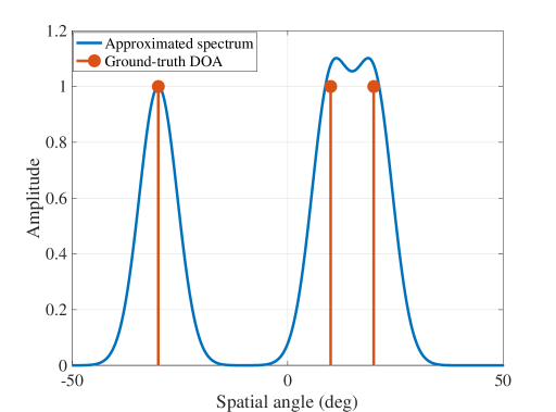
Figure 6: The refereed spatial spectrum approximated by the Gaussian functions.

With the refereed spectrum, the loss function is defined as

$$f_{\text{loss}}(\boldsymbol{\zeta})=\frac{1}{\Omega}\left\|f_{\text{ref}}(\boldsymbol{\zeta})-f_{\text{sp}}(\boldsymbol{\zeta})\right\|^{2}_{2},$$ (29)

where $f_{\text{ref}}(\boldsymbol{\zeta})\in\mathbb{R}^{\Omega\times 1}$ and $f_{\text{sp}}(\boldsymbol{\zeta})\in\mathbb{R}^{\Omega\times 1}$ are vectors with the $\omega$-th ($\omega=0,1,\dots,\Omega-1$) entry being $f_{\text{ref}}(\zeta_{\omega})$ and $f_{\text{sp}}(\zeta_{\omega})$, respectively. We define

$$\boldsymbol{\zeta}\triangleq\begin{bmatrix}\zeta_{0},\dots,\zeta_{\Omega-1}\end{bmatrix}^{\text{T}},$$ (30)

where $\Omega$ is the number of the discretized spatial angles. The SDOAnet is trained to minimize the loss function $f_{\text{loss}}(\boldsymbol{\zeta})$ in (29) by updating the network coefficients.

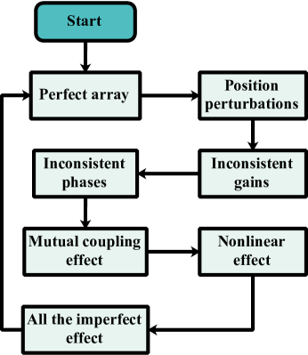
Figure 7: The training procedure for the SDOAnet.

For the practical system, the mutual coupling effect, the nonlinear effect, the inconsistent phases, the inconsistent gains, and the position perturbations are considered in this paper. The training procedure is shown in Fig. 7, and the following steps can be used to train the SDOAnet:

1. Perfect array step: The received signals using perfect array without the imperfect effect are used during the training procedure;

2. Position perturbation step: The received signals with position perturbation are used. The position perturbation is generated by a Gaussian distribution with the mean being $0$ and the standard deviation $\sigma_{\text{per}}$ selected by a uniform distribution $\sigma_{\text{per}}\in[0,\sigma_{\text{max\_per}}]$. The parameter $\sigma_{\text{max\_per}}$ can be specified in the simulation;

3. Inconsistent gains step: The inconsistent gains are considered in this step. Similarly, the inconsistent gains are generated by a zero-mean Gaussian distribution with the standard deviation $\sigma_{\text{gain}}$ being $\sigma_{\text{gain}}\in[0,\sigma_{\text{max\_gain}}]$, where $\sigma_{\text{max\_gain}}$ is specified in the simulation;

4. Inconsistent phases step: The inconsistent phases are also generated by a zero-mean Gaussian distribution with the standard deviation $\sigma_{\text{phase}}$ being $\sigma_{\text{phase}}\in[0,\sigma_{\text{max\_phase}}]$, where $\sigma_{\text{max\_phase}}$ is specified in the simulation;

5. Mutual coupling effect step: The mutual coupling effect is described by a matrix $\boldsymbol{B}$ with complex entries, and the diagonal entries are all ones. The entry at the $n$-th row and the $n^{\prime}$-th column is denoted as

   $$B_{n,n^{\prime}}=|B_{n,n^{\prime}}|e^{j\psi_{n,n^{\prime}}},$$ (31)

   and $|B_{n,n^{\prime}}|$ is determined by a uniform distribution $|B_{n,n^{\prime}}|\in[0,\sigma^{|n-n^{\prime}|}_{\text{mc}}]$ with $n\neq n^{\prime}$. The phase $\psi_{n,n^{\prime}}$ follows a uniform distribution $\psi_{n,n^{\prime}}\in[0,2\pi)$. The parameter $\sigma_{\text{mc}}$ is specified in the simulation;

6. Nonlinear effect step: The nonlinear effect is described by a nonlinear function

   $$f_{\text{nonlinear}}(x)=\tanh(x\sigma_{\text{nonlinear}}),$$ (32)

   where $\sigma_{\text{nonlinear}}$ is specified in the simulation to control the nonlinear effect;

7. All the imperfect effect step: We consider all the imperfect effects to train the network.

After training the SDOAnet in sequence according to the above steps, we start over from the first step to train the network again until the maximum number of the training procedures.

V Simulation Results

In this section, simulation results show the DOA estimation performance of the proposed SDOAnet using a practical array. The simulation results are carried out in a personal computer with MATLAB R2020b, Intel Core i5 @ 2.9 GHz processor, and 8 GB LPDDR3 @ 2133 MHz. The code about the SDOAnet is available online https://github.com/chenpengseu/SDOAnet.git, where the training codes and a pre-trained network are also provided. The network is based on PyTorch 1.4 and Python 3.7. Simulation parameters are given in Table I. We use $N=16$ antennas to receive the signals and the SDOAnet to estimate the DOA, where the number of signals is $K=3$. Moreover, the hyper-parameters for the imperfect array are also given in Table I.

TABLE I: Simulation parameters

Parameter	Value
The standard deviation in the Gaussian function	$\bar{\sigma}_{\text{G}}=100$
The batch size	$64$
The number of convolution layers	$6$
The number of filters in the convolution layer	$2$
The kernel size in the convolution layer	$3$
The learning rate	$5\times 10^{-4}$
The number of antennas	$N=16$
The number of targets	$K=3$
The distance between adjacent antennas	$0.5$ wavelength
The maximum standard deviation of position perturbation	${\sigma}_{\text{max\_per}}=0.15$
The maximum standard deviation of inconsistent gain	${\sigma}_{\text{max\_gain}}=0.5$
The maximum standard deviation of inconsistent phase	${\sigma}_{\text{max\_phase}}=0.2$
The maximum mutual coupling effect	${\sigma}_{\text{mc}}=0.06$
The nonlinear effect	${\sigma}_{\text{nonlinear}}=1.0$

First, the proposed SDOAnet contains convolution layers, and each convolution layer has convolution, batch normalization, and ReLU active function operations. In the SDOAnet, some important hyperparameters must be considered for a better DOA estimation. The first hyperparameter is the number of 1D convolution layers. In Fig. 8, we show the DOA estimation performance with different numbers of convolution layers. As shown in this figure, when the number of convolutions is $6$, a better estimation performance is achieved, so we use $6$ convolution layers in the following simulations.

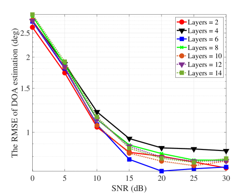
Figure 8: The DOA estimation performance with different numbers of layers.

Then, we compare the DOA estimation performance among the networks using different numbers $M_{F}$ of filters that are used in the convolution layers. For the consideration of both the estimation performance and the network complexity, better performance is achieved with $M_{F}=2$, so we will use $2$ filters in the following simulations.

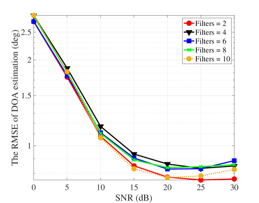
Figure 9: The DOA estimation performance with different numbers of filters.

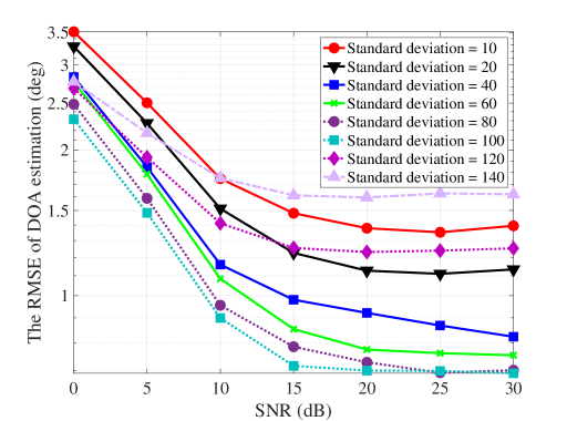
Figure 10: The DOA estimation performance with different standard deviations $\bar{\sigma}_{\text{G}}$.

In the procedure of training the SDOAnet, the referred spatial spectrum is used to measure the loss function, where we use the Gaussian functions to approximate the spatial spectrum. Hence, the standard deviation $\bar{\sigma}_{\text{G}}$ in the Gaussian function is important in approximating the spatial spectrum. We show the DOA estimation performance with different standard deviations $\bar{\sigma}_{\text{G}}$ in Fig. 10. When the standard deviation $\bar{\sigma}_{\text{G}}$ is $100$, a better DOA estimation performance is achieved, so we will use $\bar{\sigma}_{\text{G}}=100$ in the following simulation.

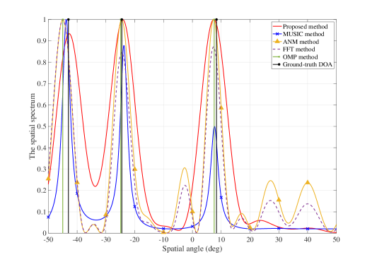
Figure 11: The spatial spectrum compared with the existing methods.

Next, based on the above SDOAnet parameters, the estimated spatial spectrum is shown in Fig. 11 for the DOA estimation and is also compared with the following existing methods:

• MUSIC method [39]: In the traditional MUSIC method, multiple snapshots are used to estimate the covariance matrix, which is used to obtain the DOA based on the eigenvalue decomposition. For a fair comparison, we use the MUSIC algorithm with only the snapshot proposed in [39], which uses both a Hankel data matrix and the Vandermonde decomposition in the MUSIC method;

• ANM method [40, 41, 42]: The ANM-based methods have been proposed for the DOA estimation and can exploit the target’s sparsity in the spatial domain. Unlike the current CS-based methods discretizing the spatial domain into grids and using a dictionary matrix for the sparse reconstruction [43, 44, 45], the ANM method estimates the DOA in the continuous domain. It can solve the off-grid problem caused by the discrete methods.

• FFT method: The FFT method is widely used in practical systems with low computational complexity. However, the resolution of the FFT method is unsatisfactory but robust to the imperfect array;

• OMP method [46, 47, 48]: The orthogonal matching pursuit (OMP) method is a CS-based method using the discretized spatial angles and has relatively low computational complexity. Hence, it has been widely used in sparse reconstruction problems.

As shown in Fig. 11, the spatial spectrum estimated by the proposed SDOAnet performs better than the MUSIC, ANM, FFT, and OMP methods. Additionally, the proposed method is based on the convolution network and has low computational complexity than the ANM and MUSIC methods. Therefore, the proposed SDOAnet is efficient in the DOA estimation problem.

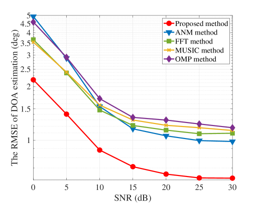
Figure 12: The DOA estimation performance with different SNRs.

Next, the DOA estimation performance under different SNRs is shown in Fig. 12, where the SNR is from $0$ dB to $30$ dB. This figure shows that a better estimation performance is achieved by the proposed method in the scenario with the imperfect array than that using ANM, FFT, MUSIC, and OMP methods. The estimation performance is measured by the root mean square error

$$\text{RMSE}=\sqrt{\frac{1}{N_{\text{sim}}K}\left\|\hat{\boldsymbol{\theta}}-\boldsymbol{\theta}\right\|^{2}_{2}},$$ (33)

where $N_{\text{sim}}$ is the number of simulations, $\hat{\boldsymbol{\theta}}$ is the estimated DOA vector, and $\boldsymbol{\theta}$ is the ground-truth DOA vector. For the SNR being $10$ dB, the RMSE of the proposed SDOAnet is about $0.70\mathrm{°}$ and that of ANM method is about $1.15\mathrm{°}$, so the RMSE improvement is about $39.13\%$. Additionally, when the SNR is $7.5$ dB, the RMSE of the proposed SDOAnet method is the same as that of the ANM method with the SNR being $15$ dB, so the SNR improvement is about $7.5$ dB.

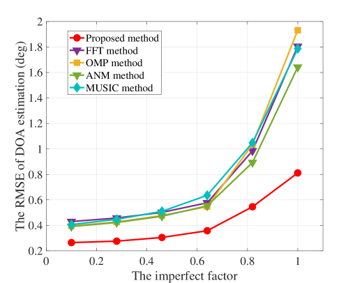
Figure 13: The DOA estimation performance with different imperfect factors.

We use an imperfect factor to measure the imperfect effect, defined as $\xi$. With the imperfect factor $\xi$, the imperfect parameters for position perturbation, inconsistent gain, inconsistent phase, mutual coupling effect, and nonlinear effect will be $\xi\sigma_{\text{max\_per}}$, $\xi\sigma_{\text{max\_gain}}$, $\xi\sigma_{\text{max\_phase}}$, $\xi\sigma_{\text{mc}}$, and $\xi\sigma_{\text{nonlinear}}$, respectively. In Fig. 13, the DOA estimation performance with different imperfect factors is shown, where a better estimation performance is achieved by the proposed SDOAnet method than the compared methods. Additionally, the proposed method works better in the scenario with a higher imperfect factor, which means that the proposed method is robust to the imperfect effect.

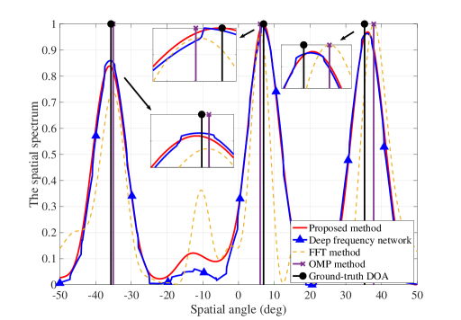
Figure 14: The spatial spectrum compared with the existing deep learning-based method.

Furthermore, a DL-based method is also proposed in [49] for the DOA estimation, named by deep frequency network, where the network’s output is the spectrum. In Fig. 14, the spatial spectrum of the proposed SDOAnet and that of the deep frequency network is given. Since the output of the deep frequency network is the spatial spectrum, the estimated spectrum is not smooth compared with the proposed SDOAnet. Hence, a better DOA estimation performance can be achieved by the SDOAnet than the deep frequency network.

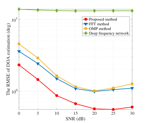
Figure 15: The DOA estimation performance compared with the existing deep learning-based method.

Finally, the DOA estimation performance under different SNRs is given in Fig. 15, where the SNR is from $0$ dB to $30$ dB. The same training data set is used for the SDOAnet and the deep frequency network. Compared with the existing methods, including the FFT method, OMP method, and deep frequency network, the proposed SDOAnet can achieve better DOA estimation performance. Therefore, the proposed method is efficient in the DOA estimation problem using the imperfect array.

VI Conclusions

The DOA estimation problem in the imperfect array has been considered in this paper. A general system model to describe the antenna position perturbations, the inconsistent gains/phases, the mutual coupling effect, the nonlinear effect, etc., have also been formulated. Then, the novel SDOAnet was proposed. Different from existing methods, the input of the SDOAnet is the raw sampled signals, and the output is a vector, which can be used to estimate the spatial spectrum. With the convolution layers, the convergence of training SDOAnet is much faster than existing DL-based methods. Simulation results show the advantages of the proposed SDOAnet in the DOA estimation problem with a practical array. Future work will focus on the theoretical analysis of the proposed SDOAnet in the DOA estimation performance.

References

- [1] J. A. Zhang, F. Liu, C. Masouros, R. W. Heath, Z. Feng, L. Zheng, and A. Petropulu, “An overview of signal processing techniques for joint communication and radar sensing,” IEEE Journal of Selected Topics in Signal Processing, vol. 15, no. 6, pp. 1295–1315, Nov. 2021.
- [2] C. Xu, B. Clerckx, S. Chen, Y. Mao, and J. Zhang, “Rate-splitting multiple access for multi-antenna joint radar and communications,” IEEE Journal of Selected Topics in Signal Processing, vol. 15, no. 6, pp. 1332–1347, Nov. 2021.
- [3] L. Zhu, S. Qiu, and Y. Han, “Combined constrained adaptive sum and difference beamforming in monopulse angle estimation,” IEEE Antennas Wireless Propag. Lett., vol. 17, no. 12, pp. 2314–2318, Dec. 2018.
- [4] J. Lin, W. Fang, Y. Wang, and J. Chen, “FSF MUSIC for joint DOA and frequency estimation and its performance analysis,” IEEE Trans. Signal Process., vol. 54, no. 12, pp. 4529–4542, Dec. 2006.
- [5] F. Yan, M. Jin, and X. Qiao, “Low-complexity DOA estimation based on compressed MUSIC and its performance analysis,” IEEE Trans. Signal Process., vol. 61, no. 8, pp. 1915–1930, Apr. 2013.
- [6] X. Zhang, L. Xu, L. Xu, and D. Xu, “Direction of departure (DOD) and direction of arrival (DOA) estimation in MIMO radar with reduced-dimension MUSIC,” IEEE Commun. Lett., vol. 14, no. 12, pp. 1161–1163, Dec. 2010.
- [7] S. Kim, D. Oh, and J. Lee, “Joint DFT-ESPRIT estimation for TOA and DOA in vehicle FMCW radars,” IEEE Antennas Wireless Propag. Lett., vol. 14, pp. 1710–1713, 2015.
- [8] J. Lin, X. Ma, S. Yan, and C. Hao, “Time-frequency multi-invariance ESPRIT for DOA estimation,” IEEE Antennas Wireless Propag. Lett., vol. 15, pp. 770–773, 2016.
- [9] X. Zhang, X. Gao, and D. Xu, “Multi-invariance ESPRIT-based blind DOA estimation for MC-CDMA with an antenna array,” IEEE Trans. Veh. Technol., vol. 58, no. 8, pp. 4686–4690, Oct. 2009.
- [10] F.-M. Han and X.-D. Zhang, “An ESPRIT-like algorithm for coherent DOA estimation,” IEEE Antennas Wireless Propag. Lett., vol. 4, pp. 443–446, 2005.
- [11] L. Wan, Y. Sun, L. Sun, Z. Ning, and J. J. P. C. Rodrigues, “Deep learning based autonomous vehicle super resolution DOA estimation for safety driving,” IEEE Trans. Intell. Transp. Syst., vol. 22, no. 7, pp. 4301–4315, Jul. 2021.
- [12] P. Chen, Z. Cao, Z. Chen, and X. Wang, “Off-grid DOA estimation using sparse Bayesian learning in MIMO radar with unknown mutual coupling,” IEEE Trans. Signal Process., vol. 67, no. 1, pp. 208–220, Jan. 2019.
- [13] J. Dai and H. C. So, “Real-valued sparse Bayesian learning for DOA estimation with arbitrary linear arrays,” IEEE Trans. Signal Process., vol. 69, pp. 4977–4990, Aug. 2021.
- [14] Y. Mao, Q. Guo, J. Ding, F. Liu, and Y. Yu, “Marginal likelihood maximization based fast array manifold matrix learning for direction of arrival estimation,” IEEE Trans. Signal Process., vol. 69, pp. 5512–5522, 2021.
- [15] J. Wan, C. Wang, P. Shen, H. Fu, and J. Zhu, “Robust and fast super-resolution SAR tomography of forests based on covariance vector sparse Bayesian learning,” IEEE Geosci. Remote Sens. Lett., vol. 19, pp. 1–5, 2022.
- [16] L. Wang, L. Zhao, S. Rahardja, and G. Bi, “Alternative to extended block sparse Bayesian learning and its relation to pattern-coupled sparse Bayesian learning,” IEEE Trans. Signal Process., vol. 66, no. 10, pp. 2759–2771, May 2018.
- [17] M. M. Hyder and K. Mahata, “Direction-of-arrival estimation using a mixed norm approximation,” IEEE Trans. Signal Process., vol. 58, no. 9, pp. 4646–4655, 2010.
- [18] R. Lu, M. Zhang, X. Liu, X. Chen, and A. Zhang, “Direction-of-arrival estimation via coarray with model errors,” IEEE Access, vol. 6, pp. 56 514–56 525, 2018.
- [19] N. Ruan, F. Wen, L. Ai, and K. Xie, “A PARAFAC decomposition algorithm for DOA estimation in colocated MIMO radar with imperfect waveforms,” IEEE Access, vol. 7, pp. 14 680–14 688, 2019.
- [20] S. Liu, Z. Zhang, and Y. Guo, “2-D DOA estimation with imperfect L-shaped array using active calibration,” IEEE Commun. Lett., vol. 25, no. 4, pp. 1178–1182, Apr. 2021.
- [21] L. Wan, Y. Sun, L. Sun, Z. Ning, and J. J. P. C. Rodrigues, “Deep learning based autonomous vehicle super resolution DOA estimation for safety driving,” IEEE Trans. Intell. Transp. Syst., vol. 22, no. 7, pp. 4301–4315, 2021.
- [22] H. Huang, J. Yang, H. Huang, Y. Song, and G. Gui, “Deep learning for super-resolution channel estimation and DOA estimation based massive MIMO system,” IEEE Trans. Veh. Technol., vol. 67, no. 9, pp. 8549–8560, 2018.
- [23] H. Lee, J. Cho, M. Kim, and H. Park, “DNN-based feature enhancement using DOA-constrained ICA for robust speech recognition,” IEEE Signal Process. Lett., vol. 23, no. 8, pp. 1091–1095, 2016.
- [24] T. N. T. Nguyen, W.-S. Gan, R. Ranjan, and D. L. Jones, “Robust source counting and DOA estimation using spatial pseudo-spectrum and convolutional neural network,” IEEE/ACM Transactions on Audio, Speech, and Language Processing, vol. 28, pp. 2626–2637, 2020.
- [25] Y. Yuan, S. Wu, M. Wu, and N. Yuan, “Unsupervised learning strategy for direction-of-arrival estimation network,” IEEE Signal Process. Lett., vol. 28, pp. 1450–1454, 2021.
- [26] L. Wu, Z. Liu, and Z. Huang, “Deep convolution network for direction of arrival estimation with sparse prior,” IEEE Signal Process. Lett., vol. 26, no. 11, pp. 1688–1692, Nov. 2019.
- [27] G. Papageorgiou, M. Sellathurai, and Y. Eldar, “Deep networks for direction-of-arrival estimation in low SNR,” IEEE Trans. Signal Process., vol. 69, pp. 3714–3729, 2021.
- [28] R. Akter, V. Doan, T. Huynh-The, and D. Kim, “RFDOA-Net: An efficient ConvNet for RF-based DOA estimation in UAV surveillance systems,” IEEE Trans. Veh. Technol., vol. 70, no. 11, pp. 12 209–12 214, Nov. 2021.
- [29] L. Wu, Z.-M. Liu, and Z.-T. Huang, “Deep convolution network for direction of arrival estimation with sparse prior,” IEEE Signal Process. Lett., vol. 26, no. 11, pp. 1688–1692, 2019.
- [30] A. M. Ahmed, U. S. K. P. M. Thanthrige, A. E. Gamal, and A. Sezgin, “Deep learning for DOA estimation in MIMO radar systems via emulation of large antenna arrays,” IEEE Commun. Lett., vol. 25, no. 5, pp. 1559–1563, 2021.
- [31] G. K. Papageorgiou, M. Sellathurai, and Y. C. Eldar, “Deep networks for direction-of-arrival estimation in low SNR,” IEEE Trans. Signal Process., vol. 69, pp. 3714–3729, 2021.
- [32] A. M. Elbir, “DeepMUSIC: Multiple signal classification via deep learning,” IEEE Sensors Lett., vol. 4, no. 4, pp. 1–4, 2020.
- [33] Z. Liu, C. Zhang, and P. Yu, “Direction-of-arrival estimation based on deep neural networks with robustness to array imperfections,” IEEE Trans. Antennas Propag., vol. 66, no. 12, pp. 7315–7327, 2018.
- [34] S. Chakrabarty and E. A. P. Habets, “Multi-speaker DOA estimation using deep convolutional networks trained with noise signals,” IEEE Journal of Selected Topics in Signal Processing, vol. 13, no. 1, pp. 8–21, Mar. 2019.
- [35] P. Chen, Z. Chen, Z. Cao, and X. Wang, “A new atomic norm for DOA estimation with gain-phase errors,” IEEE Trans. Signal Process., vol. 68, pp. 4293–4306, 2020.
- [36] Q. Wang, X. Wang, T. Dou, H. Chen, and X. Wu, “Gridless super-resolution doa estimation with unknown mutual coupling,” in ICASSP 2019 - 2019 IEEE International Conference on Acoustics, Speech and Signal Processing (ICASSP). Brighton, United Kingdom: IEEE, May 2019, pp. 4210–4214.
- [37] A. Govinda Raj and J. H. McClellan, “Single snapshot super-resolution DOA estimation for arbitrary array geometries,” IEEE Signal Process. Lett., vol. 26, no. 1, pp. 119–123, Jan. 2019.
- [38] Q. Gong, S. Ren, S. Zhong, and W. Wang, “DOA estimation using sparse array with gain-phase error based on a novel atomic norm,” Digital Signal Processing, vol. 120, p. 103266, Jan. 2022.
- [39] W. Liao and A. Fannjiang, “MUSIC for single-snapshot spectral estimation: Stability and super-resolution,” Applied and Computational Harmonic Analysis, vol. 40, no. 1, pp. 33–67, Jan. 2016.
- [40] A. Govinda Raj and J. H. McClellan, “Single snapshot super-resolution DOA estimation for arbitrary array geometries,” IEEE Signal Process. Lett., vol. 26, no. 1, pp. 119–123, Jan. 2019.
- [41] Z. Wei, W. Wang, F. Dong, and Q. Liu, “Gridless one-bit direction-of-arrival estimation via atomic norm denoising,” IEEE Commun. Lett., vol. 24, no. 10, pp. 2177–2181, Oct. 2020.
- [42] Z. Yang and L. Xie, “Enhancing sparsity and resolution via reweighted atomic norm minimization,” IEEE Trans. Signal Process., vol. 64, no. 4, pp. 995–1006, Feb. 2016.
- [43] Z. Yang, C. Zhang, J. Deng, and W. Lu, “Orthonormal expansion -minimization algorithms for compressed sensing,” IEEE Trans. Signal Process., vol. 59, no. 12, pp. 6285–6290, Dec. 2011.
- [44] Z. Tan, P. Yang, and A. Nehorai, “Joint Sparse Recovery Method for Compressed Sensing With Structured Dictionary Mismatches,” IEEE Trans. Signal Process., vol. 62, no. 19, pp. 4997–5008, Oct. 2014.
- [45] G. Yu and G. Sapiro, “Statistical compressed sensing of Gaussian mixture models,” IEEE Trans. Signal Process., vol. 59, no. 12, pp. 5842–5858, Dec. 2011.
- [46] K. Aghababaiyan, V. Shah-Mansouri, and B. Maham, “High-precision OMP-based direction of arrival estimation scheme for hybrid non-uniform array,” IEEE Commun. Lett., vol. 24, no. 2, pp. 354–357, Feb. 2020.
- [47] M. Lin, M. Xu, X. Wan, H. Liu, Z. Wu, J. Liu, B. Deng, D. Guan, and S. Zha, “Single sensor to estimate DOA with programmable metasurface,” IEEE Internet of Things Journal, vol. 8, no. 12, pp. 10 187–10 197, Jun. 2021.
- [48] Y. Chen, W. Wang, Z. Wang, and B. Xia, “A source counting method using acoustic vector sensor based on sparse modeling of DOA histogram,” IEEE Signal Process. Lett., vol. 26, no. 1, pp. 69–73, Jan. 2019.
- [49] G. Izacard, S. Mohan, and C. Fernandez-Granda, “Data-driven estimation of sinusoid frequencies,” in NeurIPS, 2019.