Conjugate Gradient Adaptive Learning with Tukey’s Biweight M-Estimate

Abstract

We propose a novel M-estimate conjugate gradient (CG) algorithm, termed Tukey’s biweight M-estimate CG (TbMCG), for system identification in impulsive noise environments. In particular, the TbMCG algorithm can achieve a faster convergence while retaining a reduced computational complexity as compared to the recursive least-squares (RLS) algorithm. Specifically, the Tukey’s biweight M-estimate incorporates a constraint into the CG filter to tackle impulsive noise environments. Moreover, the convergence behavior of the TbMCG algorithm is analyzed. Simulation results confirm the excellent performance of the proposed TbMCG algorithm for system identification and active noise control applications.

I Introduction

The $\alpha$-stable noise is an effective approach for modeling phenomena such as impulsive noise. In these scenarios, the least mean square (LMS) type algorithms, which are based on the mean square error (MSE) criterion, may fail to work [1]. To address this problem, a number of algorithms were developed [2, 3, 4, 5, 6, 7, 8, 9, 10], [11, 12, 13, 14, 15, 16, 17, 18, 19, 20, 21, 22, 23, 24, 25, 26, 27, 28, 29, 30, 31, 32, 33, 34, 35, 36, 37, 38, 39, 40, 41, 42, 43, 44, 45, 46, 47, 48, 49, 50, 51, 52, 53, 54, 55, 56, 57, 58, 59, 60, 61, 62, 63, 64, 65, 66, 67, 68, 69, 70, 71, 72, 73, 74, 75, 76, 77, 78, 79, 80, 81, 82, 83, 84, 85, 86, 87, 88, 89, 90, 91, 92, 93, 94, 95, 96, 97, 98, 99, 100]. In [101], the normalized least mean $p$th power (NLMP) algorithm was proposed, which is derived from the fractional lower order moments (FLOM) of the error signal. The M-estimate based algorithms (Huber’s and Hample’s) are effective methods to suppress the effect of impulsive noise on the filter weights [102, 103, 104, 105]. Such algorithms are essentially hybrid techniques based on $L_{1}$ and $L_{2}$-norms and several variants have been presented [106, 107, 108]. However, these algorithms can only deal with impulsive noise and cannot achieve improved performance in Gaussian scenarios. For performance improvement, the maximum correntropy criterion (MCC)-based algorithms were developed [109, 110, 111]. Such MCC method is also an M-estimator in essence [112]. It has revealed its effectiveness for non-Gaussian signal processing and has been successfully applied in many applications [113, 114, 115]. Note that the above-mentioned algorithms rely on higher-order moments and stochastic gradient (SG) methods to obtain good performance in impulsive noise.

On the other hand, the recursive least-squares (RLS) algorithm offers considerable enhancement in convergence speed and tracking capability [116, 117, 118]. Regrettably, its heavy computational load prohibits its practical use. The conjugate gradient (CG) method, which can be viewed as an alternative to RLS, is an efficient implementation for adaptive filters [119, 120]. By making use of the orthogonal search direction, such method can achieve faster convergence than the SG method [121]. Recently, the CG method and its variants have received increased attention in kernel adaptive filters [122, 123] and beamforming [124, 125]. However, there is scarce literature focused on using the CG-type algorithm for combating impulsive noise.

Motivated by the above considerations, in this paper, we propose a novel CG algorithm for combating impulsive noise. The proposed algorithm embeds the CG method inside of the Tukey’s biweight M-estimator [126, 127], resulting in the TbMCG algorithm. Compared to the above-mentioned algorithms, the proposed TbMCG algorithm is able to mitigate various noises, such as $\alpha$-stable noise, Gaussian noise, and mixed-noise. Moreover, the TbMCG algorithm can be easily extended to active noise control (ANC) system, generating a filtered-x TbMCG (FxTbMCG) algorithm. The FxTbMCG algorithm can also achieve improved performance as compared to the existing ANC algorithms.

II Problem formulation

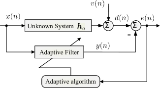
Figure 1: Diagram of the system identification problem.

Fig. 1 shows the system identification problem, where $x(n)$ denotes the input signal, $e(n)$ denotes the error signal, $\bm{h}_{o}$ denotes the weight vector of the unknown system, $v(n)$ denotes the impulsive noise, and $n$ denotes the time instant. The desired signal $d(n)$ is given by

$$d(n)={\bm{h}}^{\mathrm{T}}_{o}{\bm{x}}(n)+v(n)$$ (1)

where superscript $(\cdot)^{\mathrm{T}}$ stands for the transpose, $\bm{x}(n)=[x(n),x(n-1),\dots,x(n-L+1)]^{\mathrm{T}}$ represents the input vector, and $L$ is the filter length. The error signal $e(n)$ is defined as

$$e(n)=d(n)-y(n)=d(n)-{\bm{h}}^{\mathrm{T}}(n){\bm{x}}(n)$$ (2)

where ${\bm{h}}(n)$ is the weight vector of the adaptive filter and $y(n)={\bm{h}}^{\mathrm{T}}(n){\bm{x}}(n)$. In this paper, the impulsive noise is generated by standard symmetric $\alpha$-stable ($S\alpha S$) distribution, whose characteristic function is expressed as $\vartheta(t)=\mathrm{exp}\left\{-|t|^{\alpha}\right\}$ [7, 1], where $0<\alpha\leq 2$ is the characteristic exponent. A small value of $\alpha$ implies a strong impulsive process. Particularly, the $\alpha$-stable noise degenerates into Gaussian noise for $\alpha=2$.

III Proposed TbMCG algorithm

In this section, we derive the proposed TbMCG algorithm and detail its computational cost.

III-A Derivation of TbMCG algorithm

Considering the data set $\{\bm{x}(n),d(n)\}$, the objective function of Tukey’s biweight M-estimate with variable $e$ is expressed as [126, 127]

$${\mathcal{J}}(e)=\left\{\begin{array}[]{l}\frac{e^{2}}{c^{2}}-\frac{e^{4}}{c^{4}}+\frac{e^{6}}{3c^{6}}\;\;\;\;\;\;\;\;{\rm{if}}\;|e|\leq c\\ \frac{1}{3}\;\;\;\;\;\;\;\;\;\;\;\;\;\;\;\;\;\;\;\;\;\;\;\;\;\;\;{\rm{if}}\;|e|>c\\ \end{array}\right.$$ (3)

where $c$ is the positive constant. Recalling other M-estimate methods, Huber and Hample estimators, the non-negative threshold provides the control capability of constraining large outliers [128]. The Huber estimator is based on a convex loss function, so it has no local minima. However, it does not emphasize large errors as compared to the MSE criterion $e^{2}$. The Hample’s method, whose cost function is non-convex and can tackle extreme outliers better than the Huber one. The Tukey’s biweight (or bisquare) M-estimator shares a similar property of Hample’s M-estimator, whose objective function is also non-convex and can effectively suppress outliers. On other hand, it retains the merits of Huber’s method. It has the simplicity of an expression depending on just one tuning parameter $c$, similar to the Huber’s loss function [127].

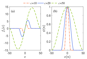
Figure 2: Evolution curves of the score function and the weighting factor.

The score function $f_{s}(e)=\partial{\mathcal{J}(e)}/\partial e$ is defined as

$$f_{s}(e)=\left\{\begin{array}[]{l}e\left[1-(\frac{e}{c})^{2}\right]^{2}\;\;\;\;\;\;\;\;\;\;{\rm{if}}\;|e|\leq c\\ 0\;\;\;\;\;\;\;\;\;\;\;\;\;\;\;\;\;\;\;\;\;\;\;\;\;\;\;\;{\rm{if}}\;|e|>c.\\ \end{array}\right.$$ (4)

To show the property of the score function, Fig. 2 (a) plots the evolution curve of $f_{s}(e)$. One can observe from this figure that the score function owns a ‘redescend’ feature, that is, when $|e|$ is large enough, $f_{s}(e)$ tends to zero. Such a phenomenon implies Tukey’s biweight M-estimate is insensitive to the outliers. Note that (4) can save computational load $f_{s}(e)=0$ when the large outliers occurs. Moreover, the score function is linear at $e=0$ in accordance with Winsor’s principle that all distributions are normal in the middle [129].

Taking the gradient of the score function w.r.t. $\bm{h}(n)$, yields

$$\frac{1}{K}\sum\limits_{n=1}^{K}\psi(n)\bm{x}(n)\bm{x}^{\mathrm{T}}(n)\bm{h}(n)=\frac{1}{K}\sum\limits_{n=1}^{K}\psi(n)d(n)\bm{x}^{\mathrm{T}}(n)$$ (5)

where $K$ denotes the sampling points and $\psi(n)$ is the weighting factor, which is expressed as

$$\psi(n)=\left\{\begin{array}[]{l}\left[1-\left(\frac{e(n)}{c}\right)^{2}\right]^{2}\;\;\;\;\;\;\;\;{\rm{if}}\;|e(n)|\leq c\\ 0\;\;\;\;\;\;\;\;\;\;\;\;\;\;\;\;\;\;\;\;\;\;\;\;\;\;\;\;\;\;{\rm{otherwise}}.\\ \end{array}\right.$$ (6)

Fig. 2 (b) depicts the curve of $\psi(n)$. As can be seen, the amplitude of $\psi(n)$ is restricted from the range of $[0,1]$, contributing to a good performance for attenuating outliers. For simplicity, define $\bm{R}=\frac{1}{K}\sum\nolimits_{n=1}^{K}\psi(n)\bm{x}(n)\bm{x}^{\mathrm{T}}(n)$ as the correlation matrix of the input signal and $\bm{\theta}=\frac{1}{K}\sum\nolimits_{n=1}^{K}\psi(n)d(n)\bm{x}^{\mathrm{T}}(n)$ as the cross-correlation vector between the desired signal and the input signal. Akin to the RLS and Newton method, the CG method can iteratively solve for the optimal solution $\bm{R}^{-1}(n)\bm{\theta}(n)$. The expression of $\bm{R}(n)$ and $\bm{\theta}(n)$ for the TbMCG algorithm is given by

$$\bm{R}(n)=\lambda\bm{R}(n-1)+\psi(n)\bm{x}(n)\bm{x}^{\mathrm{T}}(n)$$ (7)

and

$$\bm{\theta}(n)=\lambda\bm{\theta}(n-1)+\psi(n)d(n)\bm{x}^{\mathrm{T}}(n)$$ (8)

where $0\ll\lambda<1$ is the the forgetting factor. When we set $\psi(n)=1$, the TbMCG algorithm reduces to the standard CG algorithm [130].

The TbMCG algorithm computes $\bm{h}(n)$ via $\bm{h}(n-1)$ with the step size $\delta(n)$ at previous iteration $n-1$. By exploiting the orthogonality of the residuals and these previous search directions, the search linearity is independent of the previous directions. For the next solution, a new search direction, a residual, and a step size will be calculated. The residual vector can be expressed as

$$\bm{g}(n)=\bm{\theta}(n)-\bm{R}(n)\bm{h}(n)= \lambda\bm{g}(n-1)-\delta(n)\bm{R}(n)\bm{p}(n-1)$$ (9)

$$+\psi(n)\bm{x}(n)e(n).$$

Left multiplying $\bm{p}^{\mathrm{T}}(n-1)$ on both sides of (9) and taking the expectation operation on the both sides, we have

$${\mathrm{E}}\left\{\bm{p}^{\mathrm{T}}(n-1)\bm{g}(n)\right\}\approx \;\lambda{\mathrm{E}}\left\{\bm{p}^{\mathrm{T}}(n-1)\bm{g}(n)\right\}-{\mathrm{E}}\left\{\delta(n)\right\}$$ (10)

$$\times{\mathrm{E}}\left\{\bm{p}^{\mathrm{T}}(n-1)\bm{R}(n)\bm{p}(n-1)\right\}$$

$$+{\mathrm{E}}\left\{\psi(n)\right\}{\mathrm{E}}\left\{\bm{p}^{\mathrm{T}}(n-1)\right\}$$

$$\times{\mathrm{E}}\left\{\bm{x}(n)\left[d(n)-\bm{h}^{\mathrm{T}}(n)\bm{x}(n)\right]\right\}$$

where ${\mathrm{E}}\{\cdot\}$ denotes the expectation. Using the approximation results in [121], the step size $\delta(n)$ is defined by

$$\delta(n)\triangleq\eta\frac{\bm{p}^{\mathrm{T}}(n-1)\bm{g}(n-1)}{\bm{p}^{\mathrm{T}}(n-1)\bm{R}(n)\bm{p}(n-1)}$$ (11)

where $\eta>0$ is the constant parameter. Thus, the search direction vector $\bm{p}(n)$ of the TbMCG algorithm is given by

$$\bm{p}(n)=\bm{g}(n)+\beta(n)\bm{p}(n-1)$$ (12)

where $\beta(n)$ is the coefficient parameter. For the TbMCG algorithm, the Polak & Ribière (PR) approach is used [131]

$$\beta(n)=\frac{\left[\bm{g}(n)-\bm{g}(n-1)\right]^{\mathrm{T}}\bm{g}(n)}{\bm{g}^{\mathrm{T}}(n-1)\bm{g}(n-1)}.$$ (13)

At last, the update equation of the weight vector for the TbMCG algorithm is

$$\bm{h}(n)=\bm{h}(n-1)+\delta(n)\bm{p}(n).$$ (14)

TABLE I: Summary of the computational complexity.

Algorithms	$+/-$	$\times/\div$	Special instructions
LMM	$2L+4$	$2L+N_{w}+7$	0
RLS	$3L^{2}$	$4L^{2}+3L+1$	0
NMCC	$2L-1$	$2L+2$	1 exponential operation
CG	$2L^{2}+9L-4$	$3L^{2}+10L+2$	0
TbMCG	$2L^{2}+9L-3$	$3L^{2}+12L+4$	1 comparison

The computational complexity in terms of the number of operations in each iteration is analyzed in this subsection. Table I compares the computational costs of the least mean M-estimate (LMM) [103], RLS [132], normalized MCC (NMCC) [114], CG [130] and the proposed algorithms, where $N_{w}$ denotes the window length of the estimation window. Considering the conventional RLS algorithm, it is obvious that the CG algorithm has a reduced computational cost. It can be seen that the dominant terms of the complexity of the CG and TbMCG algorithms are the same or similar. To compute the weighting factor $\psi(n)$, the TbMCG algorithm requires extra 1 addition, $2L+2$ multiplications, and 1 comparison. It should be emphasized that the computational complexity of the TbMCG algorithm may be lower than the CG algorithm, since $\psi(n)=0$ when the large outliers happen and the second term of (7) and the third term of (10) can be omitted.

IV Convergence analysis

In the TbMCG algorithm, the subspace spanned by the direction vectors is equal to the subspace spanned by the residuals. Furthermore, the residual $\bm{g}(n)$ can be regarded as a linear combination of the previous residuals and $\bm{R}\bm{p}(n)$. Revisiting $\bm{p}(n+1)\in\mathcal{H}(n)$, which indicates that each new $\mathcal{H}(n+1)$ is formed from the previous $\mathcal{H}(n)$ and $\bm{R}\mathcal{H}(n)$, where $\mathcal{H}(n)$ is the Krylov subspace spanning by $\{\bm{p}(n-1)\}$

$$\mathcal{H}(n)\triangleq \;{\mathrm{span}}\left\{\bm{p}(1),\bm{R}\bm{p}(n),\ldots,\bm{R}^{n-1}\bm{p}(1)\right\}$$ (15)

$$= \;{\mathrm{span}}\left\{\bm{g}(0),\bm{R}\bm{g}(0),\ldots,\bm{R}^{n-1}\bm{g}(0)\right\}.$$

From (9), $\bm{g}(n)$ can be rewritten as $\bm{g}(n)=\bm{R}\bm{h}_{o}-\bm{R}\bm{h}(n)=\bm{R}\widetilde{\bm{h}}(n)$, where $\bm{h}_{o}$ denotes the optimal solution of the weight vector and $\widetilde{\bm{h}}(n)\triangleq\bm{h}_{o}-\bm{h}(n)$ denotes the weight error vector. Then, (15) can be rewritten by $\mathcal{H}(n)={\mathrm{span}}\left\{\bm{R}\widetilde{\bm{h}}(0),\bm{R}^{2}\widetilde{\bm{h}}(0),\ldots,\bm{R}^{n}\widetilde{\bm{h}}(0)\right\}$. Substituting $\delta(n)$ and $\bm{p}(n+1)$ into $\bm{h}(n+1)$, we have

$$\bm{h}(n+1)= \;\bm{h}(0)+[\mathcal{F}_{\bm{g}_{n}}\bm{g}(n)+\mathcal{F}_{\bm{g}_{n-1}}\bm{g}(n-1)+\ldots$$ (16)

$$+\mathcal{F}_{\bm{g}_{1}}\bm{g}(1)+\mathcal{F}_{\bm{p}_{1}}\bm{p}(1)]$$

where $\mathcal{F}_{\bm{g}_{n}}=\delta(n+1)$, $\mathcal{F}_{\bm{g}_{n-1}}=\delta(n)+\delta(n+1)\beta(n)$, $\mathcal{F}_{\bm{g}_{1}}=\delta(2)+\delta(3)\beta(2)+\delta(4)\beta(3)\beta(2)+\ldots+\delta(n+1)\beta(n)\beta(n-1)\ldots\beta(2)$, $\mathcal{F}_{\bm{p}_{1}}=\delta(1)+\delta(2)\beta(1)+\delta(3)\beta(2)\beta(1)+\delta(n+1)\beta(n)\beta(n-1)\ldots\beta(1)$. Subtracting equation (16) from $\bm{h}_{o}$, we have $\widetilde{\bm{h}}(n+1)=\widetilde{\bm{h}}(n)+\sum\limits_{j=1}^{n}\Psi(j)\bm{R}^{j}\widetilde{\bm{h}}(0)$, where $\Psi(j)$ is the linear combination of $\delta(l)$ and $\beta(k)$. It is shown that the Krylov subspace has the following property [124]:

$$\widetilde{\bm{h}}(n)=\left({\bf I}+\sum\limits_{j=1}^{n-1}\Psi(j)\bm{R}^{j}\right)\widetilde{\bm{h}}(0)$$ (17)

where $\bf I$ stands for an identity matrix. Thus, (17) is expressed in the form of a polynomial ${\mathcal{L}}_{n}(\bm{R})$, as below

$$\widetilde{\bm{h}}(n+1)={\mathcal{L}}_{n}(\bm{R})\widetilde{\bm{h}}(0)$$ (18)

where we let ${\mathcal{L}}_{0}(\bm{R})=\bf I$ due to the fact that the TbMCG algorithm cannot reach steady-state at the initial convergence. The vector $\widetilde{\bm{h}}(0)=\sum\limits_{j}\varrho_{j}\bm{\varphi}_{j}$, where $\varrho_{j}$ are the scalars not all zero and $j$ is the index number which relates to the number of the eigenvectors $\bm{\varphi}_{j}$. Considering ${\mathcal{L}}_{n}(\bm{R})\bm{\varphi}_{j}={\mathcal{L}}_{n}(\tau_{j})\bm{\varphi}_{j}$, in which $\tau_{j}$ denotes the eigenvalue to the eigenvectors $\bm{\varphi}_{j}$, (18) can be rewritten as $\widetilde{\bm{h}}(n+1)=\sum\limits_{j}\varrho_{j}{\mathcal{L}}_{n}(\tau_{j})\bm{\varphi}_{j}$ and $||\widetilde{\bm{h}}(n+1)||_{\bm{R}}^{2}=\sum\limits_{j}\varrho^{2}_{j}{\mathcal{L}}^{2}_{n}(\tau_{j})\tau_{j}$. The essence of the TbMCG algorithm is to find the minimum value of $\mathcal{L}(\tau_{j})$ during adaptation. In this regard, we have

$$\left\|\widetilde{\bm{h}}(n+1)\right\|_{\bm{R}}^{2}\leq \;\mathop{\min}\limits_{\mathcal{L}_{n}}\mathop{\max}\limits_{\tau\in\Xi(\bm{R})}{\mathcal{L}}^{2}_{n}(\tau)\sum\limits_{j}\varrho^{2}_{j}\tau_{j}$$ (19)

$$= \;\mathop{\min}\limits_{\mathcal{L}_{n}}\mathop{\max}\limits_{\tau\in\Xi(\bm{R})}{\mathcal{L}}^{2}_{n}(\tau)\left\|\widetilde{\bm{h}}(0)\right\|_{\bm{R}}^{2}$$

where $\Xi(\bm{R})$ represents the set of eigenvalues of $\bm{R}$. By using the Chebyshev polynomials [133], we arrive at

$$\left\|\widetilde{\bm{h}}(n)\right\|_{\bm{R}}^{2}\leq \;2\left(\frac{\sqrt{\zeta}-1}{\sqrt{\zeta}+1}\right)^{n}\left\|\widetilde{\bm{h}}(0)\right\|_{\bm{R}}^{2}$$ (20)

where $\zeta$ is the condition number. Owing to the fact that $\zeta$ is close to 1 for the optimal solution, and therefore $\left(\frac{\sqrt{\zeta}-1}{\sqrt{\zeta}+1}\right)^{n}$ is close to zero after iteration $n$. Hence, $\left\|\widetilde{\bm{h}}(n)\right\|_{\bm{R}}^{2}$ can converge to zero at iteration $n$.

V Simulation results

In this section, we assess the proposed TbMCG algorithm in system identification and active noise control applications.

V-A System identification

In this example, we compare the performance of the TbMCG algorithm with the LMM [103], NMCC [114], RLS [132], and CG [130] algorithms in the context of system identification. The unknown system was a ten-tap filter generated randomly. The input is an AR(1) signal with a pole at 0.5. The normalized mean-square deviation (NMSD) ${\rm{NMSD}}=20\log\left\{{\left\|\bm{h}(n)-\bm{h}_{o}\right\|}/{\bm{h}_{o}}\right\}$ is used to evaluate the performance. Simulation results are obtained by averaging the curves over 100 independent runs.

The effect of $c$ on the performance of the algorithm is shown in Fig. 3 (a) and a comparison study is conducted in Fig. 3 (b). As can be seen, $c$ behaves similar to the step-size of the LMS algorithm. A small value of $c$ can obtain small steady-state error whereas a large value of $c$ can achieve fast convergence. By considering the convergence rate and steady-state error, we select $c=20$ in this example. Moreover, it can be observed that the TbMCG algorithm has smaller NMSD for $\alpha=1.8$. We further assess the performance of those algorithms in Gaussian and mixed-noise environments, as illustrated in Fig. 4, where the LMM algorithm has high steady-state misadjustment in the Gaussian scenario and the TbMCG algorithm achieves improved performance in both cases.

Figure 3: NMSDs of the algorithms under the colored input in $\alpha=1.8$. (a) TbMCG algorithm versus different $c$ ($\lambda=0.999$, $\eta=0.001$); (b) Comparison study.

Figure 4: NMSDs of the algorithms under the colored input. (a) Gaussian noise environment ($\alpha=2$); (b) Mixed-noise (white Gaussian noise with signal-to-noise ratio (SNR)$=5$dB and impulsive noise with $\alpha=1.7$.

V-B Active noise control application

The TbMCG algorithm can be applied to the ANC problem, leading to the FxTbMCG algorithm. The RFxLMS [134], FxRLS [132] , FxlogLMS [135], and FxCG algorithms [120] are employed as benchmarks. Both primary and secondary paths are modeled by the finite impulse response (FIR) filter, obtained from [136]. To measure the reduction performance, the averaged noise reduction (ANR) is adopted [135]. We set $L=128$ for all algorithms. Since the system model of ANC is totally different from system identification, the parameter setting in this example is different from Figs. 3 and 4.

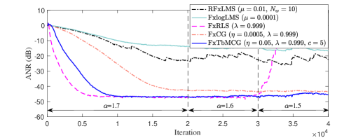
Figure 5: ANRs of five algorithms when the noise source is a time-varying $\alpha$-stable noise.

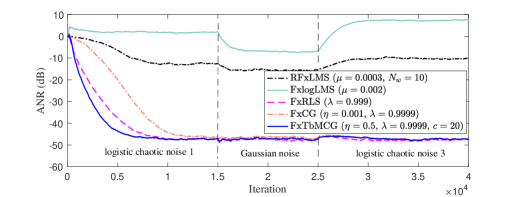
Figure 6: ANRs of five algorithms when the noise source is a time-varying noise.

First, the effect of time-varying noise sources in the attenuated performance is investigated in Figs. 5 and 6. For the highly impulsive noise, $c$ is selected to be a small value. For the noise close to a Gaussian distribution, $c$ is selected to be a large value. Fig. 5 depicts the ANRs of five algorithms when the noise source is a time-varying $\alpha$-stable noise. It can be observed that the FxRLS algorithm diverges when $\alpha=1.5$. The FxTbMCG algorithm has a fast convergence after the abrupt changes at $n=0$, $n=20,000$ and $n=30,000$, achieving a small noise residual. Then, we focus on the case that the noise source is changed at iterations 15,000 and 25,000 and the algorithms run for 40,000 iterations. The used logistic chaotic noise 1 and 3 are generated by [137]. As indicated in Fig. 6, the RFxLMS algorithm cannot track the logistic chaotic noise 3 at iteration 25,000, and the FxTbMCG algorithm achieves good tracking performance and noise residual, followed by the FxRLS algorithm.

VI Conclusions

We have proposed the TbMCG algorithm by integrating the CG method with Tukey’s biweight M-estimator for performance improvement in impulsive noise environments. Benefiting from the merits of the CG method and Tukey’s biweight M-estimator, the proposed TbMCG algorithm can effectively restrict the outliers and has moderate computational complexity. The convergence of the TbMCG algorithm has been also studied. Simulation results in the context of system identification and active noise control have demonstrated that TbMCG yields smaller steady-state error and noise residual in comparison to state-of-the-art algorithms.

We also note that for Tukey’s biweight M-estimator, $c$ is selected manually. The adaptation of $c$ is warranted for practical applications. The optimum parameter of $c$ can be obtained by the application of the methods in [138, 139, 140]. A dedicated study will be conducted in future work.

References

- [1] M. Shao and C. L. Nikias, “Signal processing with fractional lower order moments: stable processes and their applications,” Proc. IEEE, vol. 81, no. 7, pp. 986–1010, Jul. 1993.
- [2] J. Chambers and A. Avlonitis, “A robust mixed-norm adaptive filter algorithm,” IEEE Signal Process. Lett., vol. 4, no. 2, pp. 46–48, Feb. 1997.
- [3] E. V. Papoulis and T. Stathaki, “A normalized robust mixed-norm adaptive algorithm for system identification,” IEEE Signal Process. Lett., vol. 11, no. 1, pp. 56–59, Jan. 2004.
- [4] S. Al-Sayed, A. M. Zoubir, and A. H. Sayed, “Robust adaptation in impulsive noise,” IEEE Trans, Signal Process,, vol. 64, no. 11, pp. 2851–2865, Jun. 2016.
- [5] G. Aydin, O. Arikan, and A. E. Çetin, “Robust adaptive filtering algorithms for -stable random processes,” IEEE Trans. Circuits Syst. II, vol. 46, no. 2, pp. 198–202, 1999.
- [6] H. Zayyani, “Continuous mixed -norm adaptive algorithm for system identification,” IEEE Signal Process. Lett., vol. 21, no. 9, pp. 1108–1110, Sept. 2014.
- [7] L. Lu, H. Zhao, and B. Champagne, “Distributed nonlinear system identification in -stable noise,” IEEE Signal Process. Lett., vol. 25, no. 7, pp. 979–983, Jul. 2018.
- [8] H. Zayyani, “Robust minimum disturbance diffusion lms for distributed estimation,” IEEE Trans. Circuits Syst. II, vol. 68, no. 1, pp. 521–525, Jan. 2021.
- [9] H. Zayyani and A. Javaheri, “A robust generalized proportionate diffusion lms algorithm for distributed estimation,” IEEE Trans. Circuits Syst. II, vol. 68, no. 4, pp. 1552–1556, Apr. 2021.
- [10] T. Yu, W. Li, Y. Yu, and R. C. de Lamare, “Robust adaptive filtering based on exponential functional link network: Analysis and application,” IEEE Trans. Circuits Syst. II, vol. 68, no. 7, pp. 2720–2724, Jul. 2021.
- [11] R. C. de Lamare and R. Sampaio-Neto, “Adaptive reduced-rank processing based on joint and iterative interpolation, decimation, and filtering,” IEEE Transactions on Signal Processing, vol. 57, no. 7, pp. 2503–2514, 2009.
- [12] R. C. de Lamare and R. Sampaio-Neto, “Minimum mean-squared error iterative successive parallel arbitrated decision feedback detectors for ds-cdma systems,” IEEE Transactions on Communications, vol. 56, no. 5, pp. 778–789, 2008.
- [13] R. de Lamare and R. Sampaio-Neto, “Adaptive reduced-rank mmse filtering with interpolated fir filters and adaptive interpolators,” IEEE Signal Processing Letters, vol. 12, no. 3, pp. 177–180, 2005.
- [14] R. C. de Lamare, “Adaptive and iterative multi-branch mmse decision feedback detection algorithms for multi-antenna systems,” IEEE Transactions on Wireless Communications, vol. 12, no. 10, pp. 5294–5308, 2013.
- [15] R. C. de Lamare and R. Sampaio-Neto, “Reduced-rank adaptive filtering based on joint iterative optimization of adaptive filters,” IEEE Signal Processing Letters, vol. 14, no. 12, pp. 980–983, 2007.
- [16] R. C. de Lamare and R. Sampaio-Neto, “Reduced-rank space-time adaptive interference suppression with joint iterative least squares algorithms for spread-spectrum systems,” IEEE Transactions on Vehicular Technology, vol. 59, no. 3, pp. 1217–1228, 2010.
- [17] R. C. de Lamare and R. Sampaio-Neto, “Adaptive reduced-rank equalization algorithms based on alternating optimization design techniques for mimo systems,” IEEE Transactions on Vehicular Technology, vol. 60, no. 6, pp. 2482–2494, 2011.
- [18] R. Fa, R. C. de Lamare, and L. Wang, “Reduced-rank stap schemes for airborne radar based on switched joint interpolation, decimation and filtering algorithm,” IEEE Transactions on Signal Processing, vol. 58, no. 8, pp. 4182–4194, 2010.
- [19] R. C. de Lamare, M. Haardt, and R. Sampaio-Neto, “Blind adaptive constrained reduced-rank parameter estimation based on constant modulus design for cdma interference suppression,” IEEE Transactions on Signal Processing, vol. 56, no. 6, pp. 2470–2482, 2008.
- [20] P. Clarke and R. C. de Lamare, “Transmit diversity and relay selection algorithms for multirelay cooperative mimo systems,” IEEE Transactions on Vehicular Technology, vol. 61, no. 3, pp. 1084–1098, 2012.
- [21] P. Li and R. C. De Lamare, “Adaptive decision-feedback detection with constellation constraints for mimo systems,” IEEE Transactions on Vehicular Technology, vol. 61, no. 2, pp. 853–859, 2012.
- [22] Z. Yang, R. C. de Lamare, and X. Li, “¡formula formulatype=”inline”¿¡tex notation=”tex”¿¡/tex¿ ¡/formula¿-regularized stap algorithms with a generalized sidelobe canceler architecture for airborne radar,” IEEE Transactions on Signal Processing, vol. 60, no. 2, pp. 674–686, 2012.
- [23] R. de Lamare and R. Sampaio-Neto, “Adaptive mber decision feedback multiuser receivers in frequency selective fading channels,” IEEE Communications Letters, vol. 7, no. 2, pp. 73–75, 2003.
- [24] R. de Lamare, L. Wang, and R. Fa, “Adaptive reduced-rank lcmv beamforming algorithms based on joint iterative optimization of filters: Design and analysis,” Signal Processing, vol. 90, no. 2, pp. 640–652, 2010. [Online]. Available: https://www.sciencedirect.com/science/article/pii/S0165168409003466
- [25] H. Ruan and R. C. de Lamare, “Robust adaptive beamforming using a low-complexity shrinkage-based mismatch estimation algorithm,” IEEE Signal Processing Letters, vol. 21, no. 1, pp. 60–64, 2014.
- [26] R. C. de Lamare and P. S. R. Diniz, “Set-membership adaptive algorithms based on time-varying error bounds for cdma interference suppression,” IEEE Transactions on Vehicular Technology, vol. 58, no. 2, pp. 644–654, 2009.
- [27] R. de Lamare and R. Sampaio-Neto, “Blind adaptive code-constrained constant modulus algorithms for cdma interference suppression in multipath channels,” IEEE Communications Letters, vol. 9, no. 4, pp. 334–336, 2005.
- [28] S. Xu, R. C. de Lamare, and H. V. Poor, “Distributed compressed estimation based on compressive sensing,” IEEE Signal Processing Letters, vol. 22, no. 9, pp. 1311–1315, 2015.
- [29] R. C. De Lamare, R. Sampaio-Neto, and A. Hjorungnes, “Joint iterative interference cancellation and parameter estimation for cdma systems,” IEEE Communications Letters, vol. 11, no. 12, pp. 916–918, 2007.
- [30] R. Fa and R. C. De Lamare, “Reduced-rank stap algorithms using joint iterative optimization of filters,” IEEE Transactions on Aerospace and Electronic Systems, vol. 47, no. 3, pp. 1668–1684, 2011.
- [31] R. C. de Lamare and R. Sampaio-Neto, “Adaptive interference suppression for ds-cdma systems based on interpolated fir filters with adaptive interpolators in multipath channels,” IEEE Transactions on Vehicular Technology, vol. 56, no. 5, pp. 2457–2474, 2007.
- [32] R. C. De Lamare and R. Sampaio-Neto, “Blind adaptive mimo receivers for space-time block-coded ds-cdma systems in multipath channels using the constant modulus criterion,” IEEE Transactions on Communications, vol. 58, no. 1, pp. 21–27, 2010.
- [33] R. de Lamare and R. Sampaio-Neto, “Low-complexity variable step-size mechanisms for stochastic gradient algorithms in minimum variance cdma receivers,” IEEE Transactions on Signal Processing, vol. 54, no. 6, pp. 2302–2317, 2006.
- [34] A. G. D. Uchoa, C. T. Healy, and R. C. de Lamare, “Iterative detection and decoding algorithms for mimo systems in block-fading channels using ldpc codes,” IEEE Transactions on Vehicular Technology, vol. 65, no. 4, pp. 2735–2741, 2016.
- [35] R. Fa, “Multi-branch successive interference cancellation for mimo spatial multiplexing systems: design, analysis and adaptive implementation,” IET Communications, vol. 5, pp. 484–494(10), March 2011. [Online]. Available: https://digital-library.theiet.org/content/journals/10.1049/iet-com.2009.0843
- [36] N. Song, R. C. de Lamare, M. Haardt, and M. Wolf, “Adaptive widely linear reduced-rank interference suppression based on the multistage wiener filter,” IEEE Transactions on Signal Processing, vol. 60, no. 8, pp. 4003–4016, 2012.
- [37] L. T. N. Landau and R. C. de Lamare, “Branch-and-bound precoding for multiuser mimo systems with 1-bit quantization,” IEEE Wireless Communications Letters, vol. 6, no. 6, pp. 770–773, 2017.
- [38] H. Ruan and R. C. de Lamare, “Robust adaptive beamforming based on low-rank and cross-correlation techniques,” IEEE Transactions on Signal Processing, vol. 64, no. 15, pp. 3919–3932, 2016.
- [39] S. D. Somasundaram, N. H. Parsons, P. Li, and R. C. de Lamare, “Reduced-dimension robust capon beamforming using krylov-subspace techniques,” IEEE Transactions on Aerospace and Electronic Systems, vol. 51, no. 1, pp. 270–289, 2015.
- [40] T. Wang, R. C. de Lamare, and P. D. Mitchell, “Low-complexity set-membership channel estimation for cooperative wireless sensor networks,” IEEE Transactions on Vehicular Technology, vol. 60, no. 6, pp. 2594–2607, 2011.
- [41] T. Peng, R. C. de Lamare, and A. Schmeink, “Adaptive distributed space-time coding based on adjustable code matrices for cooperative mimo relaying systems,” IEEE Transactions on Communications, vol. 61, no. 7, pp. 2692–2703, 2013.
- [42] N. Song, W. U. Alokozai, R. C. de Lamare, and M. Haardt, “Adaptive widely linear reduced-rank beamforming based on joint iterative optimization,” IEEE Signal Processing Letters, vol. 21, no. 3, pp. 265–269, 2014.
- [43] R. Meng, R. C. de Lamare, and V. H. Nascimento, “Sparsity-aware affine projection adaptive algorithms for system identification,” in Sensor Signal Processing for Defence (SSPD 2011), 2011, pp. 1–5.
- [44] J. Liu and R. C. de Lamare, “Low-latency reweighted belief propagation decoding for ldpc codes,” IEEE Communications Letters, vol. 16, no. 10, pp. 1660–1663, 2012.
- [45] R. C. de Lamare and R. Sampaio-Neto, “Sparsity-aware adaptive algorithms based on alternating optimization and shrinkage,” IEEE Signal Processing Letters, vol. 21, no. 2, pp. 225–229, 2014.
- [46] L. Wang, “Constrained adaptive filtering algorithms based on conjugate gradient techniques for beamforming,” IET Signal Processing, vol. 4, pp. 686–697(11), December 2010. [Online]. Available: https://digital-library.theiet.org/content/journals/10.1049/iet-spr.2009.0243
- [47] Y. Cai, R. C. d. Lamare, and R. Fa, “Switched interleaving techniques with limited feedback for interference mitigation in ds-cdma systems,” IEEE Transactions on Communications, vol. 59, no. 7, pp. 1946–1956, 2011.
- [48] Y. Cai and R. C. de Lamare, “Space-time adaptive mmse multiuser decision feedback detectors with multiple-feedback interference cancellation for cdma systems,” IEEE Transactions on Vehicular Technology, vol. 58, no. 8, pp. 4129–4140, 2009.
- [49] Z. Shao, R. C. de Lamare, and L. T. N. Landau, “Iterative detection and decoding for large-scale multiple-antenna systems with 1-bit adcs,” IEEE Wireless Communications Letters, vol. 7, no. 3, pp. 476–479, 2018.
- [50] R. de Lamare, “Joint iterative power allocation and linear interference suppression algorithms for cooperative ds-cdma networks,” IET Communications, vol. 6, pp. 1930–1942(12), September 2012. [Online]. Available: https://digital-library.theiet.org/content/journals/10.1049/iet-com.2011.0508
- [51] P. Li and R. C. de Lamare, “Distributed iterative detection with reduced message passing for networked mimo cellular systems,” IEEE Transactions on Vehicular Technology, vol. 63, no. 6, pp. 2947–2954, 2014.
- [52] Y. Cai, R. C. de Lamare, B. Champagne, B. Qin, and M. Zhao, “Adaptive reduced-rank receive processing based on minimum symbol-error-rate criterion for large-scale multiple-antenna systems,” IEEE Transactions on Communications, vol. 63, no. 11, pp. 4185–4201, 2015.
- [53] C. T. Healy and R. C. de Lamare, “Design of ldpc codes based on multipath emd strategies for progressive edge growth,” IEEE Transactions on Communications, vol. 64, no. 8, pp. 3208–3219, 2016.
- [54] L. Wang, R. C. de Lamare, and M. Haardt, “Direction finding algorithms based on joint iterative subspace optimization,” IEEE Transactions on Aerospace and Electronic Systems, vol. 50, no. 4, pp. 2541–2553, 2014.
- [55] J. Gu, R. C. de Lamare, and M. Huemer, “Buffer-aided physical-layer network coding with optimal linear code designs for cooperative networks,” IEEE Transactions on Communications, vol. 66, no. 6, pp. 2560–2575, 2018.
- [56] S. Xu, R. C. de Lamare, and H. V. Poor, “Adaptive link selection algorithms for distributed estimation,” EURASIP J. Adv. Signal Process., vol. 86, 2015.
- [57] L. Wang, R. C. de Lamare, and Y. Long Cai, “Low-complexity adaptive step size constrained constant modulus sg algorithms for adaptive beamforming,” Signal Processing, vol. 89, no. 12, pp. 2503–2513, 2009. [Online]. Available: https://www.sciencedirect.com/science/article/pii/S0165168409001716
- [58] L. Qiu, Y. Cai, R. C. de Lamare, and M. Zhao, “Reduced-rank doa estimation algorithms based on alternating low-rank decomposition,” IEEE Signal Processing Letters, vol. 23, no. 5, pp. 565–569, 2016.
- [59] M. Yukawa, R. C. de Lamare, and R. Sampaio-Neto, “Efficient acoustic echo cancellation with reduced-rank adaptive filtering based on selective decimation and adaptive interpolation,” IEEE Transactions on Audio, Speech, and Language Processing, vol. 16, no. 4, pp. 696–710, 2008.
- [60] S. Xu, “Distributed estimation over sensor networks based on distributed conjugate gradient strategies,” IET Signal Processing, vol. 10, pp. 291–301(10), May 2016. [Online]. Available: https://digital-library.theiet.org/content/journals/10.1049/iet-spr.2015.0384
- [61] L. Landau, “Robust adaptive beamforming algorithms using the constrained constant modulus criterion,” IET Signal Processing, vol. 8, pp. 447–457(10), July 2014. [Online]. Available: https://digital-library.theiet.org/content/journals/10.1049/iet-spr.2013.0166
- [62] L. Wang and R. C. de Lamare, “Adaptive constrained constant modulus algorithm based on auxiliary vector filtering for beamforming,” IEEE Transactions on Signal Processing, vol. 58, no. 10, pp. 5408–5413, 2010.
- [63] Y. Cai and R. C. de Lamare, “Adaptive linear minimum ber reduced-rank interference suppression algorithms based on joint and iterative optimization of filters,” IEEE Communications Letters, vol. 17, no. 4, pp. 633–636, 2013.
- [64] T. G. Miller, S. Xu, R. C. de Lamare, and H. V. Poor, “Distributed spectrum estimation based on alternating mixed discrete-continuous adaptation,” IEEE Signal Processing Letters, vol. 23, no. 4, pp. 551–555, 2016.
- [65] P. Clarke and R. C. de Lamare, “Low-complexity reduced-rank linear interference suppression based on set-membership joint iterative optimization for ds-cdma systems,” IEEE Transactions on Vehicular Technology, vol. 60, no. 9, pp. 4324–4337, 2011.
- [66] S. Li, R. C. de Lamare, and R. Fa, “Reduced-rank linear interference suppression for ds-uwb systems based on switched approximations of adaptive basis functions,” IEEE Transactions on Vehicular Technology, vol. 60, no. 2, pp. 485–497, 2011.
- [67] F. G. Almeida Neto, R. C. De Lamare, V. H. Nascimento, and Y. V. Zakharov, “Adaptive reweighting homotopy algorithms applied to beamforming,” IEEE Transactions on Aerospace and Electronic Systems, vol. 51, no. 3, pp. 1902–1915, 2015.
- [68] W. S. Leite and R. C. De Lamare, “List-based omp and an enhanced model for doa estimation with non-uniform arrays,” IEEE Transactions on Aerospace and Electronic Systems, pp. 1–1, 2021.
- [69] T. Wang, R. C. de Lamare, and A. Schmeink, “Joint linear receiver design and power allocation using alternating optimization algorithms for wireless sensor networks,” IEEE Transactions on Vehicular Technology, vol. 61, no. 9, pp. 4129–4141, 2012.
- [70] R. C. de Lamare and P. S. R. Diniz, “Blind adaptive interference suppression based on set-membership constrained constant-modulus algorithms with dynamic bounds,” IEEE Transactions on Signal Processing, vol. 61, no. 5, pp. 1288–1301, 2013.
- [71] Y. Cai and R. C. de Lamare, “Low-complexity variable step-size mechanism for code-constrained constant modulus stochastic gradient algorithms applied to cdma interference suppression,” IEEE Transactions on Signal Processing, vol. 57, no. 1, pp. 313–323, 2009.
- [72] Y. Cai, R. C. de Lamare, M. Zhao, and J. Zhong, “Low-complexity variable forgetting factor mechanism for blind adaptive constrained constant modulus algorithms,” IEEE Transactions on Signal Processing, vol. 60, no. 8, pp. 3988–4002, 2012.
- [73] M. F. Kaloorazi and R. C. de Lamare, “Subspace-orbit randomized decomposition for low-rank matrix approximations,” IEEE Transactions on Signal Processing, vol. 66, no. 16, pp. 4409–4424, 2018.
- [74] R. B. Di Renna and R. C. de Lamare, “Adaptive activity-aware iterative detection for massive machine-type communications,” IEEE Wireless Communications Letters, vol. 8, no. 6, pp. 1631–1634, 2019.
- [75] H. Ruan and R. C. de Lamare, “Distributed robust beamforming based on low-rank and cross-correlation techniques: Design and analysis,” IEEE Transactions on Signal Processing, vol. 67, no. 24, pp. 6411–6423, 2019.
- [76] S. F. B. Pinto and R. C. de Lamare, “Multistep knowledge-aided iterative esprit: Design and analysis,” IEEE Transactions on Aerospace and Electronic Systems, vol. 54, no. 5, pp. 2189–2201, 2018.
- [77] Y. V. Zakharov, V. H. Nascimento, R. C. De Lamare, and F. G. De Almeida Neto, “Low-complexity dcd-based sparse recovery algorithms,” IEEE Access, vol. 5, pp. 12 737–12 750, 2017.
- [78]
- [79] S. Li and R. C. de Lamare, “Blind reduced-rank adaptive receivers for ds-uwb systems based on joint iterative optimization and the constrained constant modulus criterion,” IEEE Transactions on Vehicular Technology, vol. 60, no. 6, pp. 2505–2518, 2011.
- [80] X. Wu, Y. Cai, M. Zhao, R. C. de Lamare, and B. Champagne, “Adaptive widely linear constrained constant modulus reduced-rank beamforming,” IEEE Transactions on Aerospace and Electronic Systems, vol. 53, no. 1, pp. 477–492, 2017.
- [81] Y. Yu, H. He, T. Yang, X. Wang, and R. C. de Lamare, “Diffusion normalized least mean m-estimate algorithms: Design and performance analysis,” IEEE Transactions on Signal Processing, vol. 68, pp. 2199–2214, 2020.
- [82] R. B. Di Renna and R. C. de Lamare, “Iterative list detection and decoding for massive machine-type communications,” IEEE Transactions on Communications, vol. 68, no. 10, pp. 6276–6288, 2020.
- [83] L. Wang, “Set-membership constrained conjugate gradient adaptive algorithm for beamforming,” IET Signal Processing, vol. 6, pp. 789–797(8), October 2012. [Online]. Available: https://digital-library.theiet.org/content/journals/10.1049/iet-spr.2011.0324
- [84] P. Li, R. C. de Lamare, and R. Fa, “Multiple feedback successive interference cancellation detection for multiuser mimo systems,” IEEE Transactions on Wireless Communications, vol. 10, no. 8, pp. 2434–2439, 2011.
- [85] S. F. B. Pinto and R. C. de Lamare, “Block diagonalization precoding and power allocation for multiple-antenna systems with coarsely quantized signals,” IEEE Transactions on Communications, vol. 69, no. 10, pp. 6793–6807, 2021.
- [86] V. M. T. Palhares, A. R. Flores, and R. C. de Lamare, “Robust mmse precoding and power allocation for cell-free massive mimo systems,” IEEE Transactions on Vehicular Technology, vol. 70, no. 5, pp. 5115–5120, 2021.
- [87] A. R. Flores, R. C. De Lamare, and B. Clerckx, “Tomlinson-harashima precoded rate-splitting with stream combiners for mu-mimo systems,” IEEE Transactions on Communications, vol. 69, no. 6, pp. 3833–3845, 2021.
- [88] R. B. D. Renna and R. C. de Lamare, “Dynamic message scheduling based on activity-aware residual belief propagation for asynchronous mmtc,” IEEE Wireless Communications Letters, vol. 10, no. 6, pp. 1290–1294, 2021.
- [89] Z. Shao, L. T. N. Landau, and R. C. de Lamare, “Dynamic oversampling for 1-bit adcs in large-scale multiple-antenna systems,” IEEE Transactions on Communications, vol. 69, no. 5, pp. 3423–3435, 2021.
- [90] A. Danaee, R. C. de Lamare, and V. H. Nascimento, “Energy-efficient distributed learning with coarsely quantized signals,” IEEE Signal Processing Letters, vol. 28, pp. 329–333, 2021.
- [91] R. B. Di Renna, C. Bockelmann, R. C. de Lamare, and A. Dekorsy, “Detection techniques for massive machine-type communications: Challenges and solutions,” IEEE Access, vol. 8, pp. 180 928–180 954, 2020.
- [92] Z. Shao, L. T. N. Landau, and R. C. De Lamare, “Channel estimation for large-scale multiple-antenna systems using 1-bit adcs and oversampling,” IEEE Access, vol. 8, pp. 85 243–85 256, 2020.
- [93] F. L. Duarte and R. C. de Lamare, “Cloud-driven multi-way multiple-antenna relay systems: Joint detection, best-user-link selection and analysis,” IEEE Transactions on Communications, vol. 68, no. 6, pp. 3342–3354, 2020.
- [94] Y. Yu, H. He, T. Yang, X. Wang, and R. C. de Lamare, “Diffusion normalized least mean m-estimate algorithms: Design and performance analysis,” IEEE Transactions on Signal Processing, vol. 68, pp. 2199–2214, 2020.
- [95] A. R. Flores, R. C. de Lamare, and B. Clerckx, “Linear precoding and stream combining for rate splitting in multiuser mimo systems,” IEEE Communications Letters, vol. 24, no. 4, pp. 890–894, 2020.
- [96] X. Wang, Z. Yang, J. Huang, and R. C. de Lamare, “Robust two-stage reduced-dimension sparsity-aware stap for airborne radar with coprime arrays,” IEEE Transactions on Signal Processing, vol. 68, pp. 81–96, 2020.
- [97] Y. Yu, H. Zhao, R. C. de Lamare, Y. Zakharov, and L. Lu, “Robust distributed diffusion recursive least squares algorithms with side information for adaptive networks,” IEEE Transactions on Signal Processing, vol. 67, no. 6, pp. 1566–1581, 2019.
- [98] P. M. Vieting, R. C. de Lamare, L. Martin, G. Dartmann, and A. Schmeink, “Likelihood-based adaptive learning in stochastic state-based models,” IEEE Signal Processing Letters, vol. 26, no. 7, pp. 1031–1035, 2019.
- [99] W. Zhang, R. C. de Lamare, C. Pan, M. Chen, J. Dai, B. Wu, and X. Bao, “Widely linear precoding for large-scale mimo with iqi: Algorithms and performance analysis,” IEEE Transactions on Wireless Communications, vol. 16, no. 5, pp. 3298–3312, 2017.
- [100] Y. Cai, R. C. de Lamare, B. Champagne, B. Qin, and M. Zhao, “Adaptive reduced-rank receive processing based on minimum symbol-error-rate criterion for large-scale multiple-antenna systems,” IEEE Transactions on Communications, vol. 63, no. 11, pp. 4185–4201, 2015.
- [101] O. Arikan, M. Belge, A. E. Çetin, and E. Erzin, “Adaptive filtering approaches for non-Gaussian stable processes,” in Int. Conf. Acoust., Speech, Signal Process., vol. 2, 1995, pp. 1400–1403.
- [102] P. Petrus, “Robust huber adaptive filter,” IEEE Trans. Signal Process., vol. 47, no. 4, pp. 1129–1133, Apr. 1999.
- [103] Y. Zou, S.-C. Chan, and T.-S. Ng, “Least mean M-estimate algorithms for robust adaptive filtering in impulse noise,” IEEE Trans. Circuits Syst. II, vol. 47, no. 12, pp. 1564–1569, Dec. 2000.
- [104] Y. Zhou, S. C. Chan, and K.-L. Ho, “New sequential partial-update least mean M-estimate algorithms for robust adaptive system identification in impulsive noise,” IEEE Trans. Ind. Electron., vol. 58, no. 9, pp. 4455–4470, Sept. 2010.
- [105] S.-C. Chan, Z. G. Zhang, and Y. J. Chu, “A new transform-domain regularized recursive least M-estimate algorithm for a robust linear estimation,” IEEE Trans. Circuits Syst. II, vol. 58, no. 2, pp. 120–124, Feb. 2011.
- [106] G. Sun, M. Li, and T. C. Lim, “A family of threshold based robust adaptive algorithms for active impulsive noise control,” Appl. Acoust., vol. 97, pp. 30–36, Oct. 2015.
- [107] L. Wu and X. Qiu, “An M-estimator based algorithm for active impulse-like noise control,” Appl. Acoust., vol. 74, no. 3, pp. 407–412, Mar. 2013.
- [108] H. Zhao, Y. Chen, and S. Lv, “Robust diffusion total least mean m-estimate adaptive filtering algorithm and its performance analysis,” IEEE Trans. Circuits Syst. II, vol. 69, no. 2, pp. 654–658, Feb. 2022.
- [109] B. Chen, L. Xing, J. Liang, N. Zheng, and J. C. Príncipe, “Steady-state mean-square error analysis for adaptive filtering under the maximum correntropy criterion,” IEEE Signal Process. Lett., vol. 21, no. 7, pp. 880–884, Jul. 2014.
- [110] B. Chen and J. C. Príncipe, “Maximum correntropy estimation is a smoothed MAP estimation,” IEEE Signal Process. Lett., vol. 19, no. 8, pp. 491–494, Oct. 2012.
- [111] G. Qian, S. Wang, L. Wang, and S. Duan, “Convergence analysis of a fixed point algorithm under maximum complex correntropy criterion,” IEEE Signal Process. Lett., vol. 25, no. 12, pp. 1830–1834, Dec. 2018.
- [112] W. Liu, P. P. Pokharel, and J. C. Príncipe, “Error entropy, correntropy and M-estimation,” in Proc. Workshop Machine Learning for Signal Processing, 2006, pp. 179–184.
- [113] W. Shi, Y. Li, and B. Chen, “A separable maximum correntropy adaptive algorithm,” IEEE Trans. Circuits Syst. II, vol. 67, no. 11, pp. 2797–2801, Nov. 2020.
- [114] N. C. Kurian, K. Patel, and N. V. George, “Robust active noise control: An information theoretic learning approach,” Appl.Acoust., vol. 117, pp. 180–184, Feb. 2017.
- [115] H. Zhao, D. Liu, and S. Lv, “Robust maximum correntropy criterion subband adaptive filter algorithm for impulsive noise and noisy input,” IEEE Trans. Circuits Syst. II, vol. 62, no. 9, pp. 604–608, Feb. 2022.
- [116] Z. C. He, H. H. Ye, and E. Li, “An efficient algorithm for nonlinear active noise control of impulsive noise,” Appl. Acoust., vol. 148, pp. 366–374, May 2019.
- [117] M. Z. A. Bhotto and A. Antoniou, “New improved recursive least-squares adaptive-filtering algorithms,” IEEE Trans. Circuits Syst. I, vol. 60, no. 6, pp. 1548–1558, Jun. 2012.
- [118] M. S. Aslam, P. Shi, and C.-C. Lim, “Robust active noise control design by optimal weighted least squares approach,” IEEE Trans. Circuits Syst. I, vol. 66, no. 10, pp. 3955–3967, Oct. 2019.
- [119] C.-H. Lee, B. D. Rao, and H. Garudadri, “A sparse conjugate gradient adaptive filter,” IEEE Signal Process. Lett., vol. 27, pp. 1000–1004, Jun. 2020.
- [120] C. Teoh, K. Soh, R. Zhou, D. Tien, and V. Chan, “Active noise control of transformer noise,” in Int. Conf. Energy Manage., Power Delivery, 1998, pp. 747–753.
- [121] S. Xu, R. C. De Lamare, and H. V. Poor, “Distributed estimation over sensor networks based on distributed conjugate gradient strategies,” IET Signal Process., vol. 10, no. 3, pp. 291–301, May 2016.
- [122] M. Zhang, X. Wang, X. Chen, and A. Zhang, “The kernel conjugate gradient algorithms,” IEEE Trans. Signal Process., vol. 66, no. 16, pp. 4377–4387, Aug. 2018.
- [123] K. Xiong, H. H. Iu, and S. Wang, “Kernel correntropy conjugate gradient algorithms based on half-quadratic optimization,” IEEE Trans. Cybern., vol. 51, no. 11, pp. 5497–5510, Nov. 2021.
- [124] L. Wang and R. C. de Lamare, “Constrained adaptive filtering algorithms based on conjugate gradient techniques for beamforming,” IET Signal Process., vol. 4, no. 6, pp. 686–697, Dec. 2010.
- [125] L. Wang and R. C. de Lamare, “Set-membership constrained conjugate gradient adaptive algorithm for beamforming,” IET Signal Process., vol. 6, no. 8, pp. 789–797, Oct. 2012.
- [126] A. E. Beaton and J. W. Tukey, “The fitting of power series, meaning polynomials, illustrated on band-spectroscopic data,” Technometrics, vol. 16, no. 2, pp. 147–185, May 1974.
- [127] D. E. Tyler, Robust Statistics: Theory and Methods. Taylor & Francis, 2008.
- [128] Y. Yu, H. He, B. Chen, J. Li, Y. Zhang, and L. Lu, “M-estimate based normalized subband adaptive filter algorithm: Performance analysis and improvements,” IEEE/ACM Trans. Audio, Speech, Lang. Process., vol. 28, pp. 225–239, Oct. 2019.
- [129] J. Hardin, “Multivariate outlier detection and robust clustering with minimum covariance determinant estimation and S-estimation,” Uinversity of Califonia, pp. 1–55, 2000.
- [130] P. S. Chang and A. N. Willson, “Analysis of conjugate gradient algorithms for adaptive filtering,” IEEE Trans. Signal Process., vol. 48, no. 2, pp. 409–418, Feb. 2000.
- [131] S. Peng, Z. Wu, W. Ma, and B. Chen, “Kernel least mean square based on conjugate gradient,” in in IEEE Int. Conf. Acoust., Speech Signal Process., 2017, pp. 2796–2800.
- [132] A. H. Sayed, Adaptive Filters. John Wiley & Sons, 2011.
- [133] D. S. Watkins, Fundamentals of matrix computations. John Wiley & Sons, 2004, vol. 64.
- [134] N. V. George and G. Panda, “A robust filtered-s LMS algorithm for nonlinear active noise control,” Appl. Acoust., vol. 73, no. 8, pp. 836–841, Aug. 2012.
- [135] L. Wu, H. He, and X. Qiu, “An active impulsive noise control algorithm with logarithmic transformation,” IEEE Trans. Audio Speech Lang. Process., vol. 19, no. 4, pp. 1041–1044, May 2011.
- [136] S. M. Kuo and D. R. Morgan, Active noise control systems. Wiley, New York, 1996, vol. 4.
- [137] S. B. Behera, D. P. Das, and N. K. Rout, “Nonlinear feedback active noise control for broadband chaotic noise,” Appl. Soft Comput., vol. 15, pp. 80–87, Feb. 2014.
- [138] I. Song and P. G. Park, “A normalized least-mean-square algorithm based on variable-step-size recursion with innovative input data,” IEEE Signal Process. Lett., vol. 19, no. 12, pp. 817–820, Dec. 2012.
- [139] B. Chen, J. Liang, N. Zheng, and J. C. Príncipe, “Kernel least mean square with adaptive kernel size,” Neurocomputing, vol. 191, pp. 95–106, May 2016.
- [140] F. Huang, J. Zhang, and S. Zhang, “Adaptive filtering under a variable kernel width maximum correntropy criterion,” IEEE Trans. Circuits Syst. II, vol. 64, no. 10, pp. 1247–1251, Oct. 2017.