Learning Morphological Feature Perturbations for Calibrated Semi-Supervised Segmentation

Abstract

We propose MisMatch, a novel consistency-driven semi-supervised segmentation framework which produces predictions that are invariant to learnt feature perturbations. MisMatch consists of an encoder and a two-head decoder. One decoder pays positive attention to the foreground regions of interest (RoI) on unlabelled images thereby learning dilated features. The other decoder pays negative attention to the foreground on the same unlabelled images thereby learning eroded features. We then apply a consistency regularisation on the paired predictions. MisMatch outperforms state-of-the-art semi-supervised methods on a CT-based pulmonary vessel segmentation task and a MRI-based brain tumour segmentation task. In addition, we show that the effectiveness of MisMatch comes from better model calibration than its fully supervised learning counterpart. Code can be found here: https://github.com/moucheng2017/Learning_Morphological_Perturbation_SSL

1 Introduction

Medical image segmentation using deep learning requires expertly-labelled big data. Labels are scarce because manual labelling of medical images by experts is prohibitively expensive in both time and money. Semi-supervised learning (SSL) aims to tackle label scarcity by leveraging information in the unlabelled data. To date, SSL has relied on two key assumptions: the cluster assumption and the smoothness assumption. The cluster assumption states that data points belonging to the same cluster are more likely to be in the same class [Cahpelle et al.(2006)Cahpelle, Scholkopf, and Zien]. The smoothness assumption presumes that data points are more dense in the centre of a cluster. According to the cluster and smoothness assumptions, the optimal decision boundary should lie in a low-density region between clusters of data points. Consistency regularisation [Tarvainen and Valpola(2017)] with image-level perturbations can locate the decision boundary for image classification tasks, but does not generalise to image segmentation (Fig. 1).

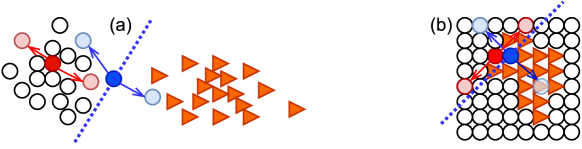
Figure 1: Illustration of consistency regularisation based SSL with data augmentation for: (a) classification; (b) segmentation. In (a), image-level perturbations with consistency learns a decision boundary in a low-density region, which can separate data points (images). This does not generalise to pixel-level data points: the decision boundary in (b) does not lie in a low-density region, and cannot separate data points (pixels).

Image-level Consistency Regularisation in Classification. Consistency regularisation has achieved state-of-the-art performance across different SSL image classification tasks, by forcing the model to produce perturbation-invariant predictions [Tarvainen and Valpola(2017), Sohn et al.(2020)Sohn, Berthelot, Li, Zhang, Carlini, Cubuk, Kurakin, Zhang, and Raffel, Berthelot et al.(2020)Berthelot, Carlini, Cubuk, Kurakin, Zhang, Raffel, and Sohn, Athiwaratkun et al.(2019)Athiwaratkun, Finzi, Izmailov, and Wilson]. This is illustrated in the cartoon of Fig. 1(a) where each data point is an image. Let’s define a perturbation on a data point as randomly changing its position in the space. A consistency loss (e.g. mean-squared error) is defined as the difference between the predictions on two different perturbations of one data point. Fig. 1(a) shows two different perturbations (red arrows) applied on the red data point lying in the high-density region, resulting in zero consistency loss as neither of the red perturbed data points crosses the decision boundary. On the other hand, when two different perturbations (blue arrows) are applied on the blue data point lying in the low-density region, the two corresponding predictions on the two perturbed blue data points will be different, leading to a valid consistency loss value which drives the decision boundary to stay in the low-density region.

Pixel-level Consistency Regularisation in Segmentation. Image segmentation operates at the pixel level, where the concept of a low-density region does not exist because pixels are uniformly and densely distributed. Hence, the assumptions behind consistency-based SSL are invalid for segmentation at the pixel level [French et al.(2020)French, Laine, Aila, Mackiewicz, and aFinalyson]. This is illustrated in the cartoon of Fig. 1(b), where the decision boundary does not correspond to the edge of the region of interest, making segmentation difficult/inaccurate. Fortunately, [Ouali et al.(2020)Ouali, Hudelot, and Tami] reported that low-density regions can be observed at the feature level and, more importantly, that low-density regions align well with the optimal decision boundaries, i.e., edges of regions of interest.

Feature-level Consistency Regularisation for Segmentation. Following the intuition above (see Fig. 1), appropriate feature-level perturbations should cross low-density regions in feature space, corresponding to the periphery of the foreground regions of interests. Naturally, we are inspired by the classic morphological operations dilation and erosion, which respectively add or remove boundary pixels to a given region of interest while preserving its shape. However, classic morphological operations are not differentiable thereby not suitable for being integrated into deep learning models. In Sec. 3.1, we show a baseline which straightforwardly applies morphological operations on the features are not ideal for consistency regularisation. A previous approach proposed hand-crafted feature perturbations [Ouali et al.(2020)Ouali, Hudelot, and Tami], which do not generalise well and not differentiable.

In this paper we introduce MisMatch, a deep, end-to-end framework for semi-supervised segmentation with consistency regularisation. The key novelty of MisMatch is to avoid the non-differentiable hand-crafted perturbations by using attention mechanisms to learn differentiable morphological perturbations at the feature level directly from the data.

2 Methods

The overarching concept behind MisMatch is to leverage different attention mechanisms to respectively dilate and erode the foreground features, which are combined in a consistency-driven framework for semi-supervised segmentation. As shown in Fig.2, MisMatch is a framework which can be integrated into any encoder-decoder based segmentation architecture.

Shape-Constrained Morphological Operations At Feature Level. Whereas classical morphological operations change the boundary of the foreground at the image level and not differentiable, our network topology is designed to learn to morph the features. We combine two concepts. First, results in [Wei et al.(2018)Wei, Xiao, Shi, Jie, Feng, and Huang, Chen et al.(2017)Chen, Papandreou, Kokkinos, Murphy, and Yuille, Luo et al.(2016)Luo, Li, Urtasun, and Zemel, Xu et al.(2020b)Xu, Oxtoby, Alexander, and Jacob] showing that Atrous convolution can enlarge foreground features by increasing false positives on the foreground boundary. Second, results in [Luo et al.(2016)Luo, Li, Urtasun, and Zemel, Xu et al.(2020b)Xu, Oxtoby, Alexander, and Jacob] showing that skip-connections can shrink foreground features. In combination, we can achieve learning-based feature perturbations with both Atrous convolution and skip-connections for consistency-driven semi-supervised segmentation.

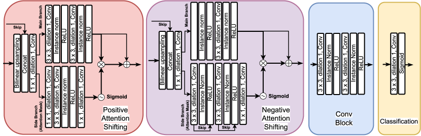
Figure 6: $f_{e}$ has 3 convolutional blocks. $f_{d1}$ has 3 PASBs followed by a classification layer. $f_{d2}$ has 3 NASBs followed by a classification layer.

Architecture of MisMatch. We use U-net [Ronneberger et al.(2015)Ronneberger, Fischer, and Brox] as backbone due to its popularity in medical imaging. Our MisMatch (Fig 2) has two components: an encoder ($f_{e}$) and a two-head decoder ($f_{d1}$ and $f_{d2}$). The first decoder ($f_{d1}$) comprises a series of Positive Attention Shifting Blocks, which dilates the foreground. The second decoder ($f_{d2}$) contains a series of Negative Attention Shifting Blocks, which erodes the foreground. The details of the architecture is in Fig.6.

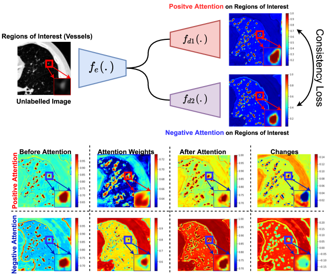
Figure 2: MisMatch learns confidence-invariant predictions on the foreground: decoder $f_{d1}$ dilates foreground features and decoder $f_{d2}$ erodes foreground features. The final prediction is the average between outputs of $f_{d1}$ and $f_{d2}$. Any encoder-decoder segmentation network could be used. We visualise the features in the last convolutional blocks in each decoder.

2.1 Positive Attention Shifting Block in $f_{d1}$

The Positive Attention Shifting Block (PASB) (candypinkPink block in Fig.6) dilates foreground features with positive attention to the foreground. Each PASB has two parallel branches, namely the main branch and the side branch. The main branch is used for processing visual information and it has the same architecture with a decoder block in a standard U-net, which comprises two consecutive convolutional layers with kernel size 3 followed by ReLU and normalisation layers. The side branch is used to generate a dilating attention mask to guide the main branch to enlarge its foreground features. To do so, the side branch uses two consecutive Atrous convolutional layers with kernel size 3 and dilation rate at 5, each followed by ReLU and a normalisation layer. In order to learn the magnitude of feature change at each pixel, we apply a Sigmoid function at the end of the side branch. We use element-wise multiplication of the output of the side branch with the output of the main branch to perturb the features of the main branch. We then apply a skip-connection on the perturbed main branch output to yield the final output of the PASB.

2.2 Negative Attention Shifting Block in $f_{d2}$

The Negative Attention Shifting Block (blue-violetPurple block in Fig.6) erodes foreground features using negative attention to the foreground. Following PASB, we design the NASB again as two parallel branches. The main branch is the same with the one in the PASB. The side branch is similar with the main branch but with a skip-connection on each convolutional layer. We also apply a Sigmoid function on the output of the side branch to learn the perturbation magnitude at each pixel. Then we multiply the learnt eroding attention mask from the side branch with the output of the main branch. We also apply a skip-connection on the perturbed main branch output to yield the final output of the NASB.

2.3 Loss Functions

We use a streaming training setting to avoid over-fitting on limited labelled data so the model doesn’t repeatedly see the labelled data during each epoch. For labelled data we apply a standard Dice loss [Milletari et al.(2016)Milletari, Navab, and Ahmadi] with the output of each decoder. For unlabelled data we apply a mean squared error loss between the outputs of the two decoders. This consistency regularisation is weighted by hyper-parameter $\alpha$ between 0.0005 to 0.004, which is also annealed during the training. Similar to SimSiam[Chen and He(2021)], we cut the gradients via detaching operation in Pytorch when applying the consistency regularisation on the two decoders.

3 Experiments

CARVE 2014 The Classification of pulmonary arteries and veins (CARVE) dataset [Charbonnier et al.(2015)Charbonnier, Brink, Ciompi, Scholten, Schaefer-Prokop, and van Rikxoort] has 10 fully annotated non-contrast low-dose thoracic CT scans. Each case has between 399 and 498 images, acquired at various resolutions between (282 x 426) to (302 x 474). 10-fold cross-validation on the 10 labelled cases is performed. In each fold, we split cases as: 1 for labelled training data, 3 for unlabelled training data, 1 for validation and 5 for testing. We have more than 2000 slices for testing. We only used slices containing more than 100 foreground pixels. We prepared datasets with differing amounts of labelled slices: 5, 10, 30, 50, 100. It is worthy to mention the most 100 slices is equal to about 10% of the whole available labelled data. We cropped 176 $\times$ 176 patches from four corners of each slice. Full label training uses 4 training cases. Normalisation was performed at case wise.

BRATS 2018 BRATS 2018 [Menze et al.(2015)Menze, Jakab, Bauer, Kalpathy-Cramer, Farahani, Kirby, Burren, Porz, Slotboom, and et al] has 210 high-grade glioma and 76 low-grade glioma MRI volumes, each case containing 155 slices. We focus on binary segmentation of whole tumours in high grade cases. We randomly selected 1 case for labelled training, 2 cases for validation and 40 cases for testing. We have 6200 slices for testing. We centre cropped slices at 176 $\times$ 176. For labelled training data, we discarded empty slices and extracted the first 20 slices containing tumours with areas of more than 5 pixels. To see the impact of the amount of unlabelled training data, we used different numbers of slices at 3100 (20 cases), 4650 (30 cases) and 6200 (40 cases) respectively. Case-wise normalisation was performed and all modalities were concatenated.

Experimental Settings We performed five sets of experiments/analysis: 1) comparisons with baselines including supervised learning and state-of-the-art semi-supervised learning approaches [Sohn et al.(2020)Sohn, Berthelot, Li, Zhang, Carlini, Cubuk, Kurakin, Zhang, and Raffel, Tarvainen and Valpola(2017), Chen et al.(2019)Chen, Bortsova, Juárez, van Tulder, and de Bruijne, Ouali et al.(2020)Ouali, Hudelot, and Tami] using either data or feature augmentation; 2) investigation of the impact of the amount of labelled data and unlabelled data on MisMatch performance; 3) ablation study of the decoder architectures; 4) ablation study on the hyper-parameter, on the CARVE dataset using 5 labelled slices; 5) calibration analysis of MisMatch, cross-validation on the CARVE with 50 labelled slices.

3.1 Baselines

The backbone is a 2D U-net [Ronneberger et al.(2015)Ronneberger, Fischer, and Brox] with 24 channels in the first encoder. To ensure a fair comparison we use the same U-net as the backbone across all baselines. The first baseline utilises supervised training on the backbone, is trained with labelled data, augmented with flipping and Gaussian noise and is denoted as “Sup1”. To investigate how unlabelled data improves performance, our second baseline “Sup2” utilises supervised training on MisMatch, with the same augmentation. Because MisMatch uses consistency regularisation, we focus on comparisons with five consistency regularisation SSL methods: 1) “mean-teacher” (MT) [Tarvainen and Valpola(2017)], with Gaussian noise, which has inspired most of the current state-of-the-art SSL methods; 2) the current state-of-the-art model called “FixMatch” (FM) [Sohn et al.(2020)Sohn, Berthelot, Li, Zhang, Carlini, Cubuk, Kurakin, Zhang, and Raffel]. To adapt FixMatch for a segmentation task, we use Gaussian noise as weak augmentation and “RandomAug” [Cubuk et al.(2020)Cubuk, Zoph, Shlens, and Le] without shearing for strong augmentation. We do not use shearing for augmentation because it impairs spatial correspondences of pixels of paired dense outputs; 3) a state-of-the-art model with multi-head decoder [Ouali et al.(2020)Ouali, Hudelot, and Tami] for segmentation (CCT), with random feature augmentation including Dropout[Srivastava et al.(2014)Srivastava, Hinton, Krizhevsky, Sutskever, and Salakhutdinov], VAT[Miyato et al.(2017)Miyato, ichi Maeda, Koyama, and Ishii] and CutOut[DeVries and Taylor(2017)], et al. This baseline is also similar to models recently developed [French et al.(2020)French, Laine, Aila, Mackiewicz, and aFinalyson, Ke et al.(2020)Ke, Qiu, Yan, and Lau]; 4) a further recent model in medical imaging [Chen et al.(2019)Chen, Bortsova, Juárez, van Tulder, and de Bruijne] using image reconstruction as an extra regularisation (MTA), augmented with Gaussian noise; 5) a U-net with two standard decoders, where we respectively apply traditional erosion and dilation on the features directly in each decoder, augmented with Gaussian noise (Morph)”. Our MisMatch model has been trained without any augmentation. See Appendix.A for details of training and implementation.

4 Results and Discussion

Labelled	Supervised		Semi-Supervised
Slices	Sup1	Sup2	MTA	MT	FM	CCT	Morph	MM
5	48.32$\pm$4.97	50.75$\pm$2.0	54.91$\pm$1.82	blue56.56$\pm$2.38	49.30$\pm$1.81	52.54$\pm$1.74	52.93$\pm$2.19	red60.25$\pm$3.77
10	53.38$\pm$2.83	55.55$\pm$4.42	57.78$\pm$3.66	blue57.99$\pm$2.57	51.53$\pm$3.72	55.25$\pm$2.52	57.08$\pm$2.96	red60.04$\pm$3.64
30	52.09$\pm$1.41	53.98$\pm$4.42	blue60.78$\pm$4.63	60.46$\pm$3.74	55.16$\pm$5.93	60.81$\pm$4.09	60.19$\pm$4.97	red63.59$\pm$4.46
50	60.69$\pm$2.51	64.79$\pm$3.46	blue68.11$\pm$3.39	67.21$\pm$3.05	62.91$\pm$6.99	65.06$\pm$3.42	64.88$\pm$3.25	red69.39$\pm$3.74
100	68.74$\pm$1.84	blue73.1$\pm$1.51	72.48$\pm$1.61	71.48$\pm$1.57	72.58$\pm$1.84	72.07$\pm$1.75	72.11$\pm$1.88	red74.83$\pm$1.52
Param. (M)	1.8	2.7	2.1	1.88	1.88	1.88	2.54	2.7
Infer.Time(s)	4.1e-3	1.8e-1	7.2e-3	4.3e-3	4.5e-3	1.5e-1	8e-3	1.8e-1
P values	9.13e-5	1.55e-2	4.5e-3	4.3e-4	1.05e-2	1.8e-3	2.2e-3	–

Table 1: MisMatch (MM) vs Baselines on CARVE. Metric is Intersection over Union (IoU): mean (std) under 10-fold cross validation. P values from Mann-Whitney U-Test against MisMatch. redRed: best model. blueBlue:2nd best model.

Unlabelled	Supervised		Semi-Supervised
Slices	Sup1	Sup2	MTA	MT	FM	CCT	Morph	MM
3100	53.74$\pm$10.19	55.76$\pm$11.03	50.53$\pm$8.76	55.29$\pm$10.21	blue57.92$\pm$12.35	56.61$\pm$11.7	53.88$\pm$9.99	red58.94$\pm$11.41
4650	53.74$\pm$10.19	55.76$\pm$11.03	47.36$\pm$6.65	blue58.32$\pm$12.07	54.29$\pm$9.69	56.94$\pm$10.93	55.82$\pm$11.03	red60.74$\pm$12.96
6200	53.74$\pm$10.19	55.76$\pm$11.03	50.11$\pm$8.00	56.92$\pm$12.20	56.78$\pm$11.39	blue57.37$\pm$11.74	54.5$\pm$9.75	red58.81$\pm$12.18

Table 2: MisMatch (MM) vs Baselines on BRATS. Metric is Intersection over Union (IoU). Each model was trained 3 times. redRed: best model. blueBlue:2nd best model.

Segmentation Performance: 1) MisMatch consistently and substantially outperforms supervised baselines, e.g. 24% improvement over Sup1 on 5 labelled slices, CARVE; 2) MisMatch consistently outperforms previous SSL methods [Sohn et al.(2020)Sohn, Berthelot, Li, Zhang, Carlini, Cubuk, Kurakin, Zhang, and Raffel, Tarvainen and Valpola(2017), Chen et al.(2019)Chen, Bortsova, Juárez, van Tulder, and de Bruijne, Ouali et al.(2020)Ouali, Hudelot, and Tami] in Table 1, across different data sets, e.g. statistical difference when 6.25% labels (100 slices comparing to 1600 slices of full label) are used on CARVE (Table 1); 3) more labelled training data consistently produces a higher mean IoU and lower standard deviation (Table 2). Visual results can be found in Fig.8 in Appendix.E.

Ablation Studies We performed ablation studies on the architecture of the decoders of MisMatch (Fig3(a)) with cross-validation on 5 labelled slices of CARVE: 1) “MM-a”, a two-headed U-net with standard convolutional blocks in decoders, this model can be seen as no feature perturbation, however, they are essentially slightly different because of random initialisation, we denote the decoder of U-net as $f_{d0}$; 2) “MM-b”, a standard decoder of U-net and a negative attention shifting decoder $f_{d2}$, this one can be seen as between no perturbation and learnt erosion perturbation; 3) “MM-c”, a standard decoder of U-net and a positive attention shifting decoder $f_{d1}$, this one can be seen as between no perturbation and learnt dilation perturbation; 4) “MM”, $f_{d1}$ and $f_{d2}$ (Ours). As shown in Fig3(b), our MisMatch (”MM”) outperforms other combinations in 8 out of 10 experiments and it performs on par with the others in the rest 2 experiments. We also tested $\alpha$ at 0, 0.0005, 0.001, 0.002, 0.004 with the same experimental setting. The optimal $\alpha$ appears at 0.002 in Fig.3(c).

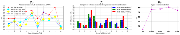
Figure 3: (a) Ablation studies on decoder architectures. (b) Performance differences between other possible decoder combinations against our used design. (c) Ablation study on the hyper-parameter alpha which weights the consistency loss. All experiments were performed on 5 labelled slices with CARVE with cross-validation

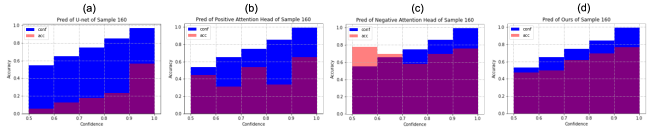
Figure 4: Reliability diagrams of one testing image. Blue: Confidence. Red: Accuracy. (a): Sup1 (Supervised learning with U-net). (b): Outputs of positive attention decoders. (c): Outputs of negative attention decoders. (d): Average outputs of the two decoders. The smaller the gap between the accuracy and the confidence, the better the network is calibrated.

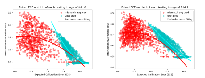
Figure 5: Expected calibration error (ECE) against segmentation performances (IoU) from cross-validation on CARVE with 50 labelled slices. $ECE=\sum_{m=1}^{M}\frac{|B_{m}|}{n}|acc(B_{m})-conf(B_{m})|$. The lower the ECE value, the better the model is calibrated.

MisMatch Is Better Calibrated We conjugate that MisMatch utilises unlabelled images to improve model calibration [Guo et al.(2017)Guo, Pleiss, Sun, and Weinberger], leading to better segmentation performance. Model calibration reflects the trustworthiness of the network predictions, which are crucial in clinical applications. Following [Guo et al.(2017)Guo, Pleiss, Sun, and Weinberger], we set $B_{m}$ as the subset of all pixels whose prediction confidence is in interval $I_{m}$. We define accuracy as how many pixels are correctly classified in each confidence interval. The accuracy of $B_{m}$ is: $acc(B_{m})=\frac{1}{|B_{m}|}\sum_{i\in B_{m}}1(\hat{y}_{i}=y_{i})$. Where $\hat{y}_{i}$ is the predicted label and $y_{i}$ is the ground truth label at pixel $i$ in $B_{m}$. The average confidence within $B_{m}$ is defined with the use of $\hat{p}_{i}$ which is the raw probability output of the network at each pixel: $conf(B_{m})=\frac{1}{|B_{m}|}\sum_{i\in B_{m}}\hat{p}_{i}$. The plot for comparing the accuracy and confidence for each interval is called Reliability map (Fig.4), the gap between the accuracy and the confidence is called expected calibration error, the smaller the gap, the better the network is calibrated. As shown in the testing result in Fig.4 and Fig.5 from experiments trained on 50 labelled slices of CARVE, MisMatch produces better calibrated predictions.

5 Conclusion

We propose MisMatch, a consistency-driven SSL framework with attention-based feature augmentation for semi-supervised segmentation of medical images. MisMatch promises strong clinical utility by reducing the number of training labels required by more than 90%: when trained on just 10% of labels, MisMatch achieves a similar performance (IoU: 75%) to models that are trained with all available labels (IoU: 77%). Future work can further explore the calibration of models to understand why consistency regularisation works.

We thank the anonymous reviewers for helping us to improve the paper quality with their constructive reviews. MCX is supported by GlaxoSmithKline (BIDS3000034123), EPSRC CDT in i4Health and UCL Engineering Dean’s Prize. NPO is supported by a UKRI Future Leaders Fellowship (MR/S03546X/1). DCA is supported by UK EPSRC grants M020533, R006032, R014019, V034537, Wellcome Trust UNS113739. JJ is supported by Wellcome Trust Clinical Research Career Development Fellowship 209,553/Z/17/Z. NPO, DCA, and JJ are supported by the NIHR UCLH Biomedical Research Centre, UK.

Appendix A Implementation

We use Adam optimiser [Kingma and Ba(2015)]. Hyper-parameters are: $\alpha=0.002$, batch size 1 (GPU memory: 2G), learning rate 2e-5, 50 epochs. Each complete training on CARVE takes about 3.8 hours. The final output is the average of the outputs of the two decoders. In testing, we take an average of models saved over the last 10 epochs across experiments. Our code is implemented using Pytorch 1.0 [Paszke et al.(2019)Paszke, Gross, Massa, Lerer, Bradbury, Chanan, Killeen, Lin, Gimelshein, Antiga, Desmaison, Kopf, Yang, DeVito, Raison, Tejani, Chilamkurthy, Steiner, Fang, Bai, and Chintala].

Appendix B Related Work

SSL in classification A recent review [Oliver et al.(2018)Oliver, Odena, Raffel, Cubuk, and Goodfellow] summarised different common SSL [Iscen et al.(2019)Iscen, Tolias, Avrithis, and Chum] [Miyato et al.(2017)Miyato, ichi Maeda, Koyama, and Ishii] [Tarvainen and Valpola(2017)] methods including entropy minimisation, label propagation methods, generative methods and consistency based methods. Entropy minimisation encourages models to produce less confident predictions on unlabelled data [Grandvalet and Bengio(2004)] [Lee(2013)]. However, entropy minimisation might overfit to the clusters of classes and fail to detect the decision boundaries of low-density regions (see Appendix E in [Oliver et al.(2018)Oliver, Odena, Raffel, Cubuk, and Goodfellow]). Label propagation methods [Iscen et al.(2019)Iscen, Tolias, Avrithis, and Chum] [Lee(2013)] aim to build a similarity graph between labelled data points and unlabelled data points in order to propagate labels through dense unlabelled data regions. Nevertheless, label propagation methods need to build and analyse their Laplacian matrices which will limit their scalability. Generative models have also been used to generate more data points in a joint optimisation of both classification of labelled data points and generative modelling [Kingma et al.(2014)Kingma, Rezende, Mohamed, and Welling]. However, the training of such a joint model can be complicated and unstable. On the other hand, consistency regularisation methods have achieved state-of-the-art performances across different benchmarks, additionally, consistency regularisation methods are simple and can easily be scaled up to large data sets. Of the consistency regularisation methods, Mean-Teacher [Tarvainen and Valpola(2017)] is the most representative example, containing two identical models which are fed with inputs augmented with different Gaussian noises. The first model learns to match the target output of the second model, while the second model uses an exponentially moving average of parameters of the first model. The state-of-the-art SSL methods [Berthelot et al.(2020)Berthelot, Carlini, Cubuk, Kurakin, Zhang, Raffel, and Sohn] [Sohn et al.(2020)Sohn, Berthelot, Li, Zhang, Carlini, Cubuk, Kurakin, Zhang, and Raffel] combines two categories: entropy minimisation and consistency regularisation.

SSL in segmentation In semi-supervised image segmentation, consistency regularisation is commonly used [Xu et al.(2020a)Xu, Lala, Gagoski, Turk, Grant, Golland, and Adalsteinsson] [Li et al.(2020)Li, Wang, Yu, and Heng] [Cui et al.(2019)Cui, Liu, Li, Guo, Li, Li, Wang, Zeng, and Ye] [Hang et al.(2020)Hang, Feng, Liang, Yu, Wang, Choi, and Qin] [Fang and Li(2020)] [French et al.(2020)French, Laine, Aila, Mackiewicz, and aFinalyson] where different data augmentation techniques are applied at the input level. Another related work [Li et al.(2018)Li, Yu, Chen, Fu, and Heng] forces the model to learn rotation invariant predictions. Apart from augmentation at the input level, recently, feature level augmentation has gained popularity for consistency based SSL segmentation [Ouali et al.(2020)Ouali, Hudelot, and Tami, Ke et al.(2020)Ke, Qiu, Yan, and Lau]. Apart from consistency regularisation methods in medical imaging, there also have been other attempts, including the use of generative models for creating pseudo data points for training [Chaitanya et al.(2019)Chaitanya, Karani, Baumgartner, Becker, Donati, and Konukoglu] [Chen et al.(2020)Chen, Qin, Qiu, Ouyang, Wang, Chen, Tarroni, Bai, and Rueckert] and different auxiliary tasks as regularisation [Kervadec et al.(2019)Kervadec, Dolz, Éric Granger, and Ayed] [Chen et al.(2019)Chen, Bortsova, Juárez, van Tulder, and de Bruijne]. Since our method is a new consistency regularisation method, we focus on comparing with state-of-the-art consistency regularisation methods.

Appendix C Detailed Architectures of Blocks of MisMatch

Appendix D More Reliability Maps

See Fig.7.

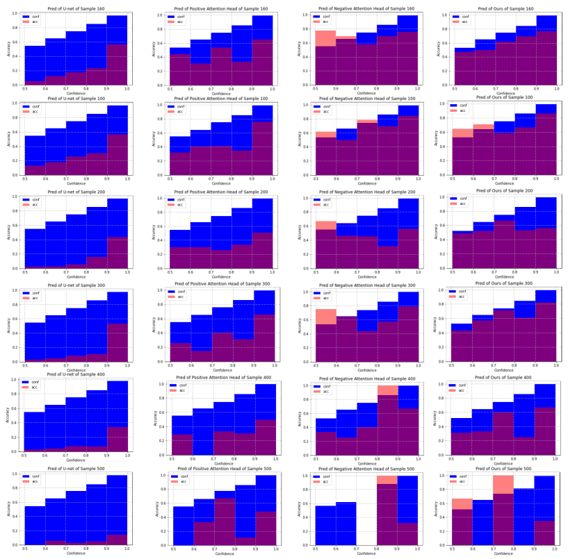
Figure 7: More reliability maps. Blue: Confidence. Red: Accuracy. Each row is on one testing image. X-axis: bins of prediction confidences. Y-axis: accuracy. Column 1: Sup1 (supervised learning with U-net). Column 2: outputs of positive attention decoders. Column 3: outputs of negative attention decoders. Column 4: average outputs of the two decoders. The smaller the gap between the accuracy and the confidence, the better the network is calibrated.

Appendix E Visual Results

See Fig.8.

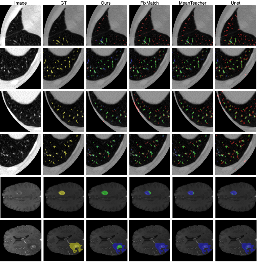
Figure 8: Visual results. Row 1-4: CARVE. Row 5-6: BRATS. Yellow: ground truth. Red: False Positive. Green: True Positives. Blue: False Negatives.

References

- [Athiwaratkun et al.(2019)Athiwaratkun, Finzi, Izmailov, and Wilson] Ben Athiwaratkun, Marc Finzi, Pavel Izmailov, and Andrew Gordon Wilson. There are many consistent explanations of unlabeled data: Why you should average. International Conference on Learning Representations (ICLR), 2019.
- [Berthelot et al.(2020)Berthelot, Carlini, Cubuk, Kurakin, Zhang, Raffel, and Sohn] David Berthelot, Nicholas Carlini, Ekin D. Cubuk, Alex Kurakin, Han Zhang, Colin Raffel, and Kihyuk Sohn. Remixmatch: Semi-supervised learning with distribution alignment and augmentation anchoring. International Conference On Learning Representation (ICLR), 2020.
- [Cahpelle et al.(2006)Cahpelle, Scholkopf, and Zien] Olivier Cahpelle, Bernhard Scholkopf, and Alexaner Zien. Semi-supervised learning. MIT Press, 2006.
- [Chaitanya et al.(2019)Chaitanya, Karani, Baumgartner, Becker, Donati, and Konukoglu] Krishna Chaitanya, Neerav Karani, Christian F. Baumgartner, Anton Becker, Olivio Donati, and Ender Konukoglu. Semi-supervised and task-driven data augmentation. Information Processing In Medical Imaging (IPMI), 2019.
- [Charbonnier et al.(2015)Charbonnier, Brink, Ciompi, Scholten, Schaefer-Prokop, and van Rikxoort] Jean-Paul Charbonnier, Monique Brink, Francesco Ciompi, Ernst T. Scholten, Cornelia M. Schaefer-Prokop, and Eva M. van Rikxoort. Automatic pulmonary artery-vein separation and classification in computed tomography using tree partitioning and peripheral vessel matching. IEEE Transaction on Medical Imaging, 2015.
- [Chen et al.(2020)Chen, Qin, Qiu, Ouyang, Wang, Chen, Tarroni, Bai, and Rueckert] Chen Chen, Chen Qin, Huaqi Qiu, Cheng Ouyang, Shuo Wang, Liang Chen, Giacomo Tarroni, Wenjia Bai, and Daniel Rueckert. Realistic adversarial data augmentation for mr image segmentation. International Conference on Medical Image Computing and Computer-Assisted Intervention (MICCAI), 2020.
- [Chen et al.(2017)Chen, Papandreou, Kokkinos, Murphy, and Yuille] Liang-Chieh Chen, George Papandreou, Iasonas Kokkinos, Kevin Murphy, and Alan L. Yuille. Deeplab: Semantic image segmentation with deep convolutional nets, atrous convolution, and fully connected crfs. Transactions on Pattern Analysis and Machine Intelligence (PAMI), 2017.
- [Chen et al.(2019)Chen, Bortsova, Juárez, van Tulder, and de Bruijne] Shuai Chen, Gerda Bortsova, Antonio García-Uceda Juárez, Gijs van Tulder, and Marleen de Bruijne. Multi-task attention-based semi-supervised learning for medical image segmentation. International Conference on Medical Image Computing and Computer-Assisted Intervention (MICCAI), 2019.
- [Chen and He(2021)] Xinlei Chen and Kaiming He. Exploring simple siamese representation learning. Computer Vision and Pattern Recognition (CVPR), 2021.
- [Cubuk et al.(2020)Cubuk, Zoph, Shlens, and Le] Ekin D. Cubuk, Barret Zoph, Jonathon Shlens, and Quoc V. Le. Randaugment: Practical automated data augmentation with a reduced search space. Neural Information Processing Systems (NeurIPS), 2020.
- [Cui et al.(2019)Cui, Liu, Li, Guo, Li, Li, Wang, Zeng, and Ye] Wenhui Cui, Yanlin Liu, Yuxing Li, Menghao Guo, Yiming Li, Xiuli Li, Tianle Wang, Xiangzhu Zeng, and Chuyang Ye. Semi-supervised brain lesion segmentation with an adapted mean teacher model. Information Processing in Medical Imaging (IPMI), 2019.
- [DeVries and Taylor(2017)] Terrance DeVries and Graham W. Taylor. Improved regularization of convolutional neural networks with cutout. arXiv:1708.04552, 2017.
- [Fang and Li(2020)] Kang Fang and Wu-Jun Li. Dmnet: Difference minimization network for semi-supervised segmentation in medical images. International Conference on Medical Image Computing and Computer-Assisted Intervention (MICCAI), 2020.
- [French et al.(2020)French, Laine, Aila, Mackiewicz, and aFinalyson] Geoff French, Samuli Laine, Timo Aila, Michal Mackiewicz, and Graham aFinalyson. Semi-supervised semantic segmentation needs strong, varied perturbations. British Machine Vision Conference (BMVC), 2020.
- [Grandvalet and Bengio(2004)] Yves Grandvalet and Yoshua Bengio. Semi-supervised learning by entropy minimization. Neural Information Processing Systems (NeurIPS), 2004.
- [Guo et al.(2017)Guo, Pleiss, Sun, and Weinberger] Chuan Guo, Geoff Pleiss, Yu Sun, and Kilian Q. Weinberger. On calibration of modern neural networks. International Conference on Machine Learning (ICML), 2017.
- [Hang et al.(2020)Hang, Feng, Liang, Yu, Wang, Choi, and Qin] Wenlong Hang, Wei Feng, Shuang Liang, Lequan Yu, Qiong Wang, Kup-Sze Choi, and Jing Qin. Local and global structure-aware entropy regularized mean teacher model for 3d left atrium segmentation. International conference on medical image computing and computer assisted intervention (MICCAI), 2020.
- [Iscen et al.(2019)Iscen, Tolias, Avrithis, and Chum] Ahmet Iscen, Giorgos Tolias, Yannis Avrithis, and Ondˇrej Chum. Label propagation for deep semi-supervised learning. Computer Vision and Pattern Recognition (CVPR), 2019.
- [Ke et al.(2020)Ke, Qiu, Yan, and Lau] Zhanghan Ke, Di Qiu, Qiong Yan, and Rynson W.H. Lau. Guided collaborative training for pixel-wise semi-supervised learning. European Conference on Computer Vision (ECCV), 2020.
- [Kervadec et al.(2019)Kervadec, Dolz, Éric Granger, and Ayed] Hoel Kervadec, Jose Dolz, Éric Granger, and Ismail Ben Ayed. Curriculum semi-supervised segmentation. International Conference on Medical Image Computing and Computer-Assisted Intervention (MICCAI), 2019.
- [Kingma and Ba(2015)] Diederik P. Kingma and Jimmy Ba. Adam: A method for stochastic optimization. International Conference on Learning Representation (ICLR), 2015.
- [Kingma et al.(2014)Kingma, Rezende, Mohamed, and Welling] Diederik P. Kingma, Danilo J. Rezende, Shakir Mohamed, and Max Welling. Semi-supervised learning with deep generative models. Advanced in Neural Information Processing System (NeurIPS), 2014.
- [Lee(2013)] Dong-Hyun Lee. Pseudo-label : The simple and efficient semi-supervised learning method for deep neural networks. ICML workshop on Challenges in Representation Learning, 2013.
- [Li et al.(2020)Li, Wang, Yu, and Heng] Kang Li, Shujun Wang, Lequan Yu, and Pheng-Ann Heng. Dual-teacher: Integrating intra-domain and inter-domain teachers for annotation-efficient cardiac segmentation. International Conference on Medical Image Computing and Computer-Assisted Intervention (MICCAI), 2020.
- [Li et al.(2018)Li, Yu, Chen, Fu, and Heng] Xiaomeng Li, Lequan Yu, Hao Chen, Chi Wing Fu, and Pheng Ann Heng. Semi-supervised skin lesion segmentation via transformation consistent self-ensembling model. British Machine Vision Conference (BMVC), 2018.
- [Luo et al.(2016)Luo, Li, Urtasun, and Zemel] Wenjie Luo, Yujia Li, Raquel Urtasun, and Richard Zemel. Understanding the effective receptive field in deep convolutional neural networks. Neural Information Processing Systems (NeurIPS), 2016.
- [Menze et al.(2015)Menze, Jakab, Bauer, Kalpathy-Cramer, Farahani, Kirby, Burren, Porz, Slotboom, and et al] Bjoern H. Menze, Andras Jakab, Stefan Bauer, Jayashree Kalpathy-Cramer, Keyvan Farahani, Justin Kirby, Yuliya Burren, Nicole Porz, Johannes Slotboom, and et al. The multimodal brain tumor image segmentation benchmark (brats). IEEE Transaction on Medical Imaging, 2015.
- [Milletari et al.(2016)Milletari, Navab, and Ahmadi] Fausto Milletari, Nassir Navab, and Seyed-Ahmad Ahmadi. V-net: Fully convolutional neural networks for volumetric medical image segmentation. International Conference on 3D Vision (3DV), 2016.
- [Miyato et al.(2017)Miyato, ichi Maeda, Koyama, and Ishii] Takeru Miyato, Shin ichi Maeda, Masanori Koyama, and Shin Ishii. Virtual adversarial training: A regularization method for supervised and semi-supervised learning. IEEE Transactions on Pattern Analysis and Machine Intelligence, 2017.
- [Oliver et al.(2018)Oliver, Odena, Raffel, Cubuk, and Goodfellow] Avital Oliver, Augustus Odena, Colin Raffel, Ekin D. Cubuk, and Ian J. Goodfellow. Realistic evaluation of deep semi-supervised learning algorithms. Neural Information Processing Systems (NeurIPS), 2018.
- [Ouali et al.(2020)Ouali, Hudelot, and Tami] Yassine Ouali, Céline Hudelot, and Myriam Tami. Semi-supervised semantic segmentation with cross-consistency training. Computer Vision and Pattern Recognition (CVPR), 2020.
- [Paszke et al.(2019)Paszke, Gross, Massa, Lerer, Bradbury, Chanan, Killeen, Lin, Gimelshein, Antiga, Desmaison, Kopf, Yang, DeVito, Raison, Tejani, Chilamkurthy, Steiner, Fang, Bai, and Chintala] Adam Paszke, Sam Gross, Francisco Massa, Adam Lerer, James Bradbury, Gregory Chanan, Trevor Killeen, Zeming Lin, Natalia Gimelshein, Luca Antiga, Alban Desmaison, Andreas Kopf, Edward Yang, Zachary DeVito, Martin Raison, Alyhkan Tejani, Sasank Chilamkurthy, Benoit Steiner, Lu Fang, Junjie Bai, and Soumith Chintala. Pytorch: An imperative style, high-performance deep learning library. Neural Information Processing System (NeurIPS), 2019.
- [Ronneberger et al.(2015)Ronneberger, Fischer, and Brox] Olaf Ronneberger, Philipp Fischer, and Thomas Brox. U-net: Convolutional networks for biomedical image segmentations. International conference on medical image computing and computer assisted intervention (MICCAI), 2015.
- [Sohn et al.(2020)Sohn, Berthelot, Li, Zhang, Carlini, Cubuk, Kurakin, Zhang, and Raffel] Kihyuk Sohn, David Berthelot, Chun-Liang Li, Zizhao Zhang, Nicholas Carlini, Ekin D. Cubuk, Alex Kurakin, Han Zhang, and Colin Raffel. Fixmatch: Simplifying semi-supervised learning with consistency and confidence. Neural Information Processing Systems (NeurIPS), 2020.
- [Srivastava et al.(2014)Srivastava, Hinton, Krizhevsky, Sutskever, and Salakhutdinov] Nitish Srivastava, Geoffrey Hinton, Alex Krizhevsky, Ilya Sutskever, and Ruslan Salakhutdinov. Dropout: A simple way to prevent neural networks from overfitting. Journal of Machine Learning Research, 2014.
- [Tarvainen and Valpola(2017)] Antti Tarvainen and Harri Valpola. Mean teachers are better role models: Weight-averaged consistency targets improve semi-supervised deep learning results. Neural Information Processing Systems (NeurIPS), 2017.
- [Wei et al.(2018)Wei, Xiao, Shi, Jie, Feng, and Huang] Yunchao Wei, Huaxin Xiao, Honghui Shi, Zequn Jie, Jiashi Feng, and Thomas S Huang. Revisiting dilated convolution: A simple approach for weakly- and semisupervised semantic segmentation. Computer Vision and Pattern Recognition (CVPR), 2018.
- [Xu et al.(2020a)Xu, Lala, Gagoski, Turk, Grant, Golland, and Adalsteinsson] Junshen Xu, Sayeri Lala, Borjan Gagoski, Esra Abaci Turk, P. Ellen Grant, Polina Golland, and Elfar Adalsteinsson. Semi-supervised learning for fetal brain mri quality assessment with roi consistency. International Conference on Medical Image Computing and Computer-Assisted Intervention (MICCAI), 2020a.
- [Xu et al.(2020b)Xu, Oxtoby, Alexander, and Jacob] Mou-Cheng Xu, Neil P Oxtoby, Daniel C Alexander, and Joseph Jacob. Learning to pay attention to mistakes. British Machine Vision Conference (BMVC), 2020b.