A Class of Two-Timescale Stochastic EM Algorithms for Nonconvex Latent Variable Models

Abstract

The Expectation-Maximization (EM) algorithm is a popular choice for learning latent variable models. Variants of the EM have been initially introduced by Neal and Hinton (1998), using incremental updates to scale to large datasets, and by Wei and Tanner (1990); Delyon et al. (1999), using Monte Carlo (MC) approximations to bypass the intractable conditional expectation of the latent data for most nonconvex models. In this paper, we propose a general class of methods called Two-Timescale EM Methods based on a two-stage approach of stochastic updates to tackle an essential nonconvex optimization task for latent variable models. We motivate the choice of a double dynamic by invoking the variance reduction virtue of each stage of the method on both sources of noise: the index sampling for the incremental update and the MC approximation. We establish finite-time and global convergence bounds for nonconvex objective functions. Numerical applications on various models such as deformable template for image analysis or nonlinear models for pharmacokinetics are also presented to illustrate our findings.

1 Introduction

Learning latent variable models is critical for many important modern machine learning problems, see for instance McLachlan and Krishnan (2007) for references. We formulate the training of this type of model as the following empirical risk minimization problem:

$$\begin{split}\min_{{\bm{\theta}}\in\Theta}~{}\overline{{\textsf{L}}}({\bm{\theta}})\mathrel{\mathop{:}}={\textsf{L}}({\bm{\theta}})+\operatorname{r}({\bm{\theta}})\quad\text{with}~{}~{}{\textsf{L}}({\bm{\theta}})=\frac{1}{n}\sum_{i=1}^{n}{\textsf{L}}_{i}({\bm{\theta}})\mathrel{\mathop{:}}=\frac{1}{n}\sum_{i=1}^{n}\big{\{}-\log g(y_{i};{\bm{\theta}})\big{\}}\;,\end{split}$$ (1)

where $\{y_{i}\}_{i=1}^{n}$ are observations, $\Theta\subset\mathbb{R}^{d}$ is the parameters set and $\operatorname{r}:\Theta\rightarrow\mathbb{R}$ is a smooth regularizer. The objective $\overline{{\textsf{L}}}({\bm{\theta}})$ is possibly nonconvex and is assumed to be lower bounded. In the latent data model, the likelihood $g(y_{i};{\bm{\theta}})$, is the marginal distribution of the complete data likelihood, noted $f(z_{i},y_{i};{\bm{\theta}})$, such that for a compact set $\mathsf{Z}\subset\mathbb{R}^{p}$

$$g(y_{i};{\bm{\theta}})=\int_{\mathsf{Z}}f(z_{i},y_{i};{\bm{\theta}})\mu(\mathrm{d}z_{i})\,,$$ (2)

where $\{z_{i}\}_{i=1}^{n}$ are the vectors of latent variables associated to the observations $\{y_{i}\}_{i=1}^{n}$. In this paper, we assume that the complete data likelihood belongs to the curved exponential family (Efron, 1975), i.e.,

$$f(z_{i},y_{i};{\bm{\theta}})=h(z_{i},y_{i})\exp(\big{\langle}S(z_{i},y_{i})\,,\,\phi({\bm{\theta}})\big{\rangle}-\psi({\bm{\theta}}))\;,$$ (3)

where $\psi({\bm{\theta}})$, $h(z_{i},y_{i})$ are scalar functions, $\phi({\bm{\theta}})\in\mathbb{R}^{k}$ is a vector function, and $\{S(z_{i},y_{i})\in\mathbb{R}^{k}\}_{i=1}^{n}$ is the vector of sufficient statistics. Batch EM (Dempster et al., 1977; Wu, 1983), the method of reference for (1), is comprised of two steps. At iteration $k$, the E-step computes the conditional expectation of the sufficient statistics of (3), noted $\overline{{\mathbf{s}}}({\bm{\theta}})=\frac{1}{n}\sum_{i=1}^{n}\overline{{\mathbf{s}}}_{i}({\bm{\theta}})$, where for all ${\bm{\theta}}\in\Theta$ and $i\in[n]$, where $[n]\mathrel{\mathop{:}}=\{1,\cdots,n\}$:

$$\overline{{\mathbf{s}}}_{i}(\hat{{\bm{\theta}}}^{(k)})\mathrel{\mathop{:}}=\int_{\mathsf{Z}}S(z_{i},y_{i})p(z_{i}|y_{i};\hat{{\bm{\theta}}}^{(k)})\mu(\mathrm{d}z_{i})\;,$$ (4)

and the M-step is given by

$$\hat{{\bm{\theta}}}^{(k+1)}=\overline{{\bm{\theta}}}(\overline{{\mathbf{s}}}(\hat{{\bm{\theta}}}^{(k)}))\mathrel{\mathop{:}}=\mathop{\mathrm{arg\,min}}_{\vartheta\in\Theta}~{}\big{\{}\operatorname{r}(\vartheta)+\psi(\vartheta)-\big{\langle}\overline{{\mathbf{s}}}(\hat{{\bm{\theta}}}^{(k)})\,,\,\phi(\vartheta)\big{\rangle}\big{\}}\;.$$ (5)

There are two main caveats of such a method: (a) with the explosion of data, the first step of the EM is computationally inefficient as it requires, at each iteration, a full pass over the dataset; and (b) the complexity of modern models makes the expectation in (4) intractable. Both of these constraints occur in the E-step of the EM algorithm, see the integral and finite sum structure of (4) and we tackle them jointly in this contribution.

1.1 Prior Work

Inspired by stochastic optimization procedures, Neal and Hinton (1998); Cappé and Moulines (2009) developed respectively an incremental and an online variant of the E-step in models where the expectation is computable, and were then extensively used and studied in Nguyen et al. (2020); Liang and Klein (2009); Cappé (2011). Some improvements of those methods have been provided and analyzed, globally and in finite-time, in Karimi et al. (2019) where variance reduction techniques taken from the optimization literature have been efficiently applied to scale the EM algorithm to large datasets. Follow-up studies on variance reduced stochastic EM include Fort et al. (2020, 2021). Regarding the computation of the expectation under the posterior distribution, the Monte Carlo EM (MCEM) has been introduced in Wei and Tanner (1990) where a Monte Carlo (MC) approximation for this expectation is computed. Its convergence is established in Fort and Moulines (2003). A variant of that algorithm is the Stochastic Approximation of the EM (SAEM) in Delyon et al. (1999) leveraging the power of Robbins-Monro update (Robbins and Monro, 1951) to ensure pointwise convergence of the vector of estimated parameters using a decreasing stepsize rather than increasing the number of MC samples. The MCEM and the SAEM have been successfully applied in mixed effects models (McCulloch, 1997; Hughes, 1999; Baey et al., 2016) or to do inference for joint modeling of time-to-event data coming from clinical trials in Chakraborty and Das (2010), unsupervised clustering in Ng and McLachlan (2003), variational inference of graphical models in Blei et al. (2017) among other applications. An incremental variant of the SAEM was proposed in Kuhn et al. (2020) but its analysis is limited to asymptotic consideration. Gradient-based methods have been developed and analyzed in Zhu et al. (2017) but remain out of the scope of this paper as they tackle the high-dimensionality issue.

1.2 Contributions

This paper introduces and analyzes a new class of methods which purpose is to update two proxies for the target expected quantities in a two-timescale manner. Those approximated quantities are then used to optimize the objective function (1) for challenging examples (nonlinear) and settings (large-scale) using the M-step of the EM algorithm. Our main contributions can be summarized as follows:

• We propose a two-timescale method based on (i) stochastic approximation (SA), to alleviate the burden of computing MC approximations, and on (ii) incremental updates, scaling to large datasets. We describe the edges of each level of our method based on variance reduction arguments. Such class of algorithms has two advantages. First, it naturally leverages variance reduction and Robbins-Monro type of updates to tackle large-scale and highly nonconvex learning tasks. Then, it gives a simple formulation as a scaled-gradient method which makes the analysis and implementation accessible.

• We also establish global (independent of the initialization) and finite-time (true at each iteration) upper bounds on a classical sub-optimality condition (Jain and Kar, 2017; Ghadimi and Lan, 2013), i.e., the second order moment of the gradient of the objective function. We discuss the double dynamic of those bounds due to the two-timescale property of our algorithm update and we theoretically show the advantages of introducing variance reduction in a stochastic approximation (Robbins and Monro, 1951) scheme.

• Our theoretical findings include MC sampling noise contrary to existing studies related to the EM where the expectations are computed exactly. Adding a layer of MC approximation and the SA step to reduce its variance introduce new challenges that need careful considerations and account for the originality of our research paper, both on the algorithmic and theoretical plans.

• Numerical experiments are presented in this contribution on a variety of models and datasets. In particular, we provide empirical insights on the edges of our method for learning latent variable models in image analysis and pharmacokinetics.

In Section 2 we formalize both incremental and Monte Carlo variants of the EM. We introduce our two-timescale class of EM (TTSEM) algorithms for which we derive several statistical guarantees in Section 3 for possibly nonconvex functions. Section 4 corresponds to the sketches of the proofs for our main results. Section 5 is devoted to the numerical experiments showing the benefits of our methods on several tasks and datasets. Proofs and additional experimental details are deferred to the Appendix.

2 Two-Timescale Stochastic EM Algorithms

We recall and formalize in this section the different methods found in the literature that aim at solving the intractable expectation problem and the large-scale problem. We then introduce our class of stochastic methods that efficiently tackles the optimization problem in (1).

2.1 Monte Carlo Integration and Stochastic Approximation

As mentioned in the introduction, for complex and possibly nonconvex models, the expectation under the posterior distribution defined in (4) is not tractable. In that case, the first solution involves computing a Monte Carlo integration of that expectation. For all $i\in[n]$, draw $M$ samples, noted $\{z_{i,m}\sim p(z_{i}|y_{i};{\bm{\theta}})\}_{m=1}^{M}$, and compute the MC integration, noted $\tilde{S}$, of $\overline{{\mathbf{s}}}({\bm{\theta}})\mathrel{\mathop{:}}=\frac{1}{n}\sum_{i=1}^{n}\overline{{\mathbf{s}}}_{i}({\bm{\theta}})$ where each of its component is defined by (4):

$$\textrm{MC-step}:~{}\tilde{S}\mathrel{\mathop{:}}=\frac{1}{n}\sum_{i=1}^{n}\frac{1}{M}\sum_{m=1}^{M}S(z_{i,m},y_{i})\;.$$ (6)

Then, update the parameter via the maximization function $\overline{{\bm{\theta}}}(\tilde{S})$. This algorithm, called the MCEM (Wei and Tanner, 1990), bypasses the intractable expectation issue but is rather computationally expensive. Indeed, in order to reach pointwise convergence, the number of samples $M$ needs to be increasingly large. An alternative to the MCEM is to use a Robbins-Monro (RM) type of update, see Robbins and Monro (1951). We denote, for $k>0$, the number of samples $M_{k}$ and the approximation by $\tilde{S}^{(k+1)}$:

$$\begin{split}\tilde{S}^{(k+1)}\mathrel{\mathop{:}}=\frac{1}{n}\sum_{i=1}^{n}\tilde{S}^{(k+1)}_{i}=\frac{1}{n}\sum_{i=1}^{n}\frac{1}{M_{k}}\sum_{m=1}^{M_{k}}S(z_{i,m}^{(k)},y_{i})\;,\end{split}$$ (7)

where for $m\in[M_{k}]$, $z_{i,m}^{(k)}\sim p(z_{i}|y_{i};{\bm{\theta}}^{(k)})$. Then, the RM update of the statistics $\hat{{\mathbf{s}}}^{(k+1)}$ reads:

$$\textrm{SA-step}:~{}\hat{{\mathbf{s}}}^{(k+1)}=\hat{{\mathbf{s}}}^{(k)}+\gamma_{k+1}(\tilde{S}^{(k+1)}-\hat{{\mathbf{s}}}^{(k)})\;,$$ (8)

where $\{\gamma_{k}\}_{k>1}\in(0,1)$ is a sequence of decreasing stepsizes to ensure asymptotic convergence. The combination of (7) and (8) is called the Stochastic Approximation of the EM (SAEM) and has been shown to converge to a maximum likelihood of the observations under very general conditions, see Delyon et al. (1999) for a proof of convergence. In simple scenarios, the samples $\{z_{i,m}\}_{m=1}^{M}$ are conditionally independent and identically distributed with distribution $p(z_{i},{\bm{\theta}})$. Nevertheless, in most cases, since the loss function between the observed data $y_{i}$ and the latent variable $z_{i}$ can be nonconvex, sampling exactly from this distribution is not an option and the MC batch is sampled by Markov Chain Monte Carlo (MCMC) algorithm (Brooks et al., 2011; Meyn and Tweedie, 2012). It is proved in Kuhn and Lavielle (2004) that (8) converges almost surely when coupled with an MCMC procedure.

Role of the stepsize $\gamma_{k}$: The sequence of decreasing positive integers $\{\gamma_{k}\}_{k>1}$ controls the convergence of the algorithm. It is inefficient to start with small values for the stepsize $\gamma_{k}$ and large values for the number of simulations $M_{k}$. Rather, it is recommended that one decreases $\gamma_{k}$, as in $\gamma_{k}=1/k^{\alpha}$, with $\alpha\in(0,1)$, and keeps a constant and small number of samples $M_{k}$, hence bypassing the computationally involved sampling step in (6). In practice, $\gamma_{k}$ is set equal to $1$ during the first few iterations to let the iterates explore the parameter space without memory and converge quickly to a neighborhood of the target estimate. The Stochastic Approximation is performed during the remaining iterations ensuring the almost sure convergence of the vector of estimates. This Robbins-Monro type of update constitutes the first level of our algorithm, needed to temper the variance and noise introduced by the Monte Carlo integration. In the next section, we derive variants of this algorithm to adapt to the sheer size of data of modern applications and formalize the second level of our class of two-timescale EM methods.

2.2 Incremental and Two-Timescale Stochastic EM Methods

Efficient strategies to scale to large datasets include incremental (Neal and Hinton, 1998) and variance reduced (Johnson and Zhang, 2013; Chen et al., 2018) methods. We explicit a general update that covers those latter variants and that represents the second level of our algorithm, i.e., the incremental update of the noisy statistics $\tilde{S}^{(k+1)}$ in (7). Instead of computing its full batch $\tilde{S}^{(k+1)}$ as in (7), the MC approximation is incrementally evaluated through $S_{\textrm{tts}}^{(k+1)}$ as:

$$\textrm{Inc-step}:~{}S_{\textrm{tts}}^{(k+1)}=S_{\textrm{tts}}^{(k)}+\rho_{k+1}({\bm{\mathcal{S}}}^{(k+1)}-S_{\textrm{tts}}^{(k)})\;.$$ (9)

Note that $\{\rho_{k}\}_{k>1}\in(0,1)$ is a sequence of stepsizes, ${\bm{\mathcal{S}}}^{(k)}$ is a proxy for $\tilde{S}^{(k)}$ defined in (7). When $\rho_{k}=1$ and ${\bm{\mathcal{S}}}^{(k)}=\tilde{S}^{(k)}$, i.e., computed in a full batch manner as in (7), then we recover the SAEM algorithm, if $\rho_{k}=1$, $\gamma_{k}=1$ and ${\bm{\mathcal{S}}}^{(k)}=\tilde{S}^{(k)}$, then we recover the MCEM algorithm.

Two-Timescale Stochastic EM methods: We introduce the general method derived using the two variance reduction techniques described above. Beforehand, we list in Table 1, variants of the Inc-step, stated in (9), of Algorithm 1 for the quantity ${\bm{\mathcal{S}}}^{(k+1)}$, at iteration $k>0$. Our paper introduces two new variants of the iSAEM (incremental SAEM), introduced by Kuhn et al. (2020), namely vrTTEM (variance reduced SAEM) and fiTTEM (fast incremental SAEM) in order to accelerate the convergence of the parameters. For each method, we define a random index noted $i_{k}\in[n]$ and drawn at iteration $k$, and $\tau_{i}^{k}=\max\{k^{\prime}:i_{k^{\prime}}=i,~{}k^{\prime}<k\}$ as the iteration index where $i\in[n]$ is last drawn prior to iteration $k$.

Table 1 Proxies for the Incremental-step (9)

1:  iSAEM $\hskip 19.91684pt{\bm{\mathcal{S}}}^{(k+1)}={\bm{\mathcal{S}}}^{(k)}+n^{-1}(\tilde{S}_{i_{k}}^{(k)}-\tilde{S}_{i_{k}}^{(\tau_{i_{k}}^{k})})$

2:  vrTTEM $\hskip 14.22636pt{\bm{\mathcal{S}}}^{(k+1)}=S_{\textrm{tts}}^{(\ell(k))}+(\tilde{S}_{i_{k}}^{(k)}-\tilde{S}_{i_{k}}^{(\ell(k))})$

3:  fiTTEM $\hskip 17.07182pt{\bm{\mathcal{S}}}^{(k+1)}=\overline{{\bm{\mathcal{S}}}}^{(k)}+(\tilde{S}_{i_{k}}^{(k)}-\tilde{S}_{i_{k}}^{(t_{i_{k}}^{k})})\quad$ and $\quad\overline{{\bm{\mathcal{S}}}}^{(k+1)}=\overline{{\bm{\mathcal{S}}}}^{(k)}+n^{-1}(\tilde{S}_{j_{k}}^{(k)}-\tilde{S}_{j_{k}}^{(t_{j_{k}}^{k})})$

Note that the proposed fiTTEM update, Line 3 in Table 1, draws two independent and uniform indices $(i_{k},j_{k})\in[n]$. Thus, we define $t_{j}^{k}=\{k^{\prime}:j_{k^{\prime}}=j,k^{\prime}<k\}$ to be the iteration index where the sample $j\in[n]$ is last drawn as $j_{k}$ prior to iteration $k$ in addition to $\tau_{i}^{k}$ which was defined w.r.t. $i_{k}$. We recall that $\tilde{S}_{i_{k}}^{(k)}\mathrel{\mathop{:}}=\frac{1}{M_{k}}\sum_{m=1}^{M_{k}}S(z_{i_{k},m}^{(k)},y_{i_{k}})$ where $z_{i_{k},m}^{(k)}$ are samples drawn from $p(z_{i_{k}}|y_{i_{k}};{\bm{\theta}}^{(k)})$. The stepsize in (9) is set to $\rho_{k+1}=1$ for the iSAEM method initializing with ${\bm{\mathcal{S}}}^{(0)}=\tilde{S}^{(0)}$; $\rho_{k+1}=\rho$ is constant for the vrTTEM and fiTTEM. Note that we initialize with $\overline{{\bm{\mathcal{S}}}}^{(0)}=\tilde{S}^{(0)}$ for the fiTTEM which can be seen as a slightly modified version of SAGA inspired by Reddi et al. (2016). For vrTTEM  we set an epoch size of $m$ and we define $\ell(k)\mathrel{\mathop{:}}=m\lfloor k/m\rfloor$ as the first iteration number in the epoch that iteration $k$ is in. Then, our general class of methods, see Algorithm 1, leverages both levels (8) and (9) in order to output a vector of fitted parameters $\hat{{\bm{\theta}}}^{({K}_{f})}$ where ${K}_{f}$ is the total number of iterations.

Algorithm 1 Two-Timescale Stochastic EM methods.

1:  Input: $\hat{{\bm{\theta}}}^{(0)}\leftarrow{\bm{\theta}}_{0}$, $\hat{{\mathbf{s}}}^{(0)}\leftarrow\tilde{S}^{(0)}$, $\{\gamma_{k}\}_{k>0}$, $\{\rho_{k}\}_{k>0}$ and ${K}_{f}\in\mathbb{N}^{*}$.

2:  Set the terminating iteration number, $K\in\{0,\dots,{K}_{f}-1\}$, as a discrete r.v. with:

$$P(K=k)=\frac{\gamma_{k}}{\sum_{\ell=0}^{{K}_{f}-1}\gamma_{\ell}}=\frac{\gamma_{k}}{{P}_{m}}\;.$$ (10)

3:  for $k=0,1,2,\dots,{K}_{f}-1$ do

4:     Draw index $i_{k}\in[n]$ uniformly (and $j_{k}\in[n]$ for fiTTEM).

5:     Compute $\tilde{S}_{i_{k}}^{(k)}$ using the MC-step (6), for the drawn indices.

6:     Compute the surrogate sufficient statistics ${\bm{\mathcal{S}}}^{(k+1)}$ using Lines 1, 2, and 3 in Table 1.

7:     Compute $\hat{{\mathbf{s}}}^{(k+1)}$ and $S_{\textrm{tts}}^{(k+1)}$ using resp. (8) and (9):

$$\begin{split}&S_{\textrm{tts}}^{(k+1)}=S_{\textrm{tts}}^{(k)}+\rho_{k+1}({\bm{\mathcal{S}}}^{(k+1)}-S_{\textrm{tts}}^{(k)})\;,\\ &\hat{{\mathbf{s}}}^{(k+1)}=\hat{{\mathbf{s}}}^{(k)}+\gamma_{k+1}(S_{\textrm{tts}}^{(k+1)}-\hat{{\mathbf{s}}}^{(k)})\;.\end{split}$$ (11)

8:     Update $\hat{{\bm{\theta}}}^{(k+1)}=\overline{{\bm{\theta}}}(\hat{{\mathbf{s}}}^{(k+1)})$ via the M-step (5).

9:  end for

The update in (11) is said to have a two-timescale property as the stepsizes satisfy $\lim_{k\to\infty}\gamma_{k}/\rho_{k}<1$ such that $\tilde{S}^{(k+1)}$ is updated at a faster time-scale, determined by $\rho_{k+1}$, than $\hat{{\mathbf{s}}}^{(k+1)}$, determined by $\gamma_{k+1}$. The next section introduces the main results of this paper and establishes global and finite-time bounds for the different updates of our scheme.

3 Finite Time Analysis of Two-Timescale EMs

Notations reminder: $\tilde{S}$ represents the MC approximation of its expected counterpart $\overline{{\mathbf{s}}}$ at index $i\in[n]$. $S_{\textrm{tts}}$ denotes the variance-reduced quantity in (9), related to the stepsize $\rho$ (assumed constant here), and leveraging the incrementally updated quantity ${\bm{\mathcal{S}}}$ via Table 1. The quantity noted $\hat{{\mathbf{s}}}$ stands for the sufficient statistics resulting from the RM procedure in (8) and is updated using the SA stepsize $\gamma$.

Following Cappé and Moulines (2009), it can be shown that stationary points of the objective function (1) corresponds to the stationary points of the following nonconvex Lyapunov function:

$$\min_{{{\mathbf{s}}}\in\mathsf{S}}~{}V({{\mathbf{s}}})\mathrel{\mathop{:}}=\overline{\textsf{L}}(\overline{{\bm{\theta}}}({\mathbf{s}}))=\frac{1}{n}\sum_{i=1}^{n}{\textsf{L}}_{i}(\overline{{\bm{\theta}}}({\mathbf{s}}))+\operatorname{r}(\overline{{\bm{\theta}}}({\mathbf{s}}))\;,$$ (12)

that we propose to study in this paper and where ${\textsf{L}}_{i}$ is defined in (1).

3.1 Assumptions and Intermediate Lemmas

In order to derive the desired convergence guarantees, several important assumptions are given below:

A​​ 1.

The sets $\mathsf{Z},\mathsf{S}$ are compact set of $\mathbb{R}^{p}$. Besides, there exist constants $C_{\mathsf{S}},C_{\mathsf{Z}}$ such that

$$\textstyle\begin{split}C_{\mathsf{S}}\mathrel{\mathop{:}}=\max_{{\mathbf{s}},{\mathbf{s}}^{\prime}\in\mathsf{S}}\|{\mathbf{s}}-{\mathbf{s}}^{\prime}\|<\infty\quad\textrm{and}\quad C_{\mathsf{Z}}\mathrel{\mathop{:}}=\max_{i\in[n]}\int_{\mathsf{Z}}|S(z,y_{i})|\mu(\mathrm{d}z)<\infty.\end{split}$$

A​​ 2.

For any $i\in[n]$, $z\in\mathsf{Z}$, ${\bm{\theta}},{\bm{\theta}}^{\prime}\in{\rm int}(\Theta)^{2}$, where ${\rm int}(\Theta)$ denotes the interior of $\Theta$, we have $\big{|}p(z|y_{i};{\bm{\theta}})-p(z|y_{i};{\bm{\theta}}^{\prime})\big{|}\leq\operatorname{L}_{p}\|{\bm{\theta}}-{\bm{\theta}}^{\prime}\|$.

We recall that we consider the curved exponential family such that the objective function satisfies:

A​​ 3.

For any $\bm{s}\in\mathsf{S}$, the function ${\bm{\theta}}\mapsto L(s,{\bm{\theta}})\mathrel{\mathop{:}}=\operatorname{r}({\bm{\theta}})+\psi({\bm{\theta}})-\big{\langle}{\mathbf{s}}\,,\,\phi({\bm{\theta}})\big{\rangle}$ admits a unique global minimum $\overline{{\bm{\theta}}}({{\mathbf{s}}})\in{\rm int}(\Theta)$. In addition, $\operatorname{J}_{\phi}^{{\bm{\theta}}}(\overline{{\bm{\theta}}}({\mathbf{s}}))$, the Jacobian of the function $\phi$ at ${\bm{\theta}}$, is full rank, $\operatorname{L}_{p}$-Lipschitz and $\overline{{\bm{\theta}}}({\mathbf{s}})$ is $\operatorname{L}_{t}$-Lipschitz.

We denote by $\operatorname{H}_{L}^{{\bm{\theta}}}({\mathbf{s}},{\bm{\theta}})$ the Hessian (w.r.t to ${\bm{\theta}}$ for a given value of ${\mathbf{s}}\in\mathsf{S}$) of the function ${\bm{\theta}}\mapsto L({\mathbf{s}},{\bm{\theta}})=\operatorname{r}({\bm{\theta}})+\psi({\bm{\theta}})-\big{\langle}{\mathbf{s}}\,,\,\phi({\bm{\theta}})\big{\rangle}$, and define

$$\operatorname{B}({\mathbf{s}})\mathrel{\mathop{:}}=\operatorname{J}_{\phi}^{{\bm{\theta}}}(\overline{{\bm{\theta}}}({{\mathbf{s}}}))(\operatorname{H}_{L}^{{\bm{\theta}}}({{\mathbf{s}}},\overline{{\bm{\theta}}}({{\mathbf{s}}})))^{-1}\operatorname{J}_{\phi}^{{\bm{\theta}}}(\overline{{\bm{\theta}}}({{\mathbf{s}}}))^{\top}\,.$$

A​​ 4.

It holds that $\upsilon_{\max}\mathrel{\mathop{:}}=\sup_{{\mathbf{s}}\in\mathsf{S}}\|\operatorname{B}({\mathbf{s}})\|<\infty$ and $0<\upsilon_{\min}\mathrel{\mathop{:}}=\inf_{{\mathbf{s}}\in\mathsf{S}}\lambda_{\rm min}(\operatorname{B}({\mathbf{s}}))$. There exists a constant $\operatorname{L}_{b}$ such that for all ${\mathbf{s}},{\mathbf{s}}^{\prime}\in\mathsf{S}^{2}$, we have $\|\operatorname{B}({\mathbf{s}})-\operatorname{B}({\mathbf{s}}^{\prime})\|\leq\operatorname{L}_{b}\|{{\mathbf{s}}}-{{\mathbf{s}}}^{\prime}\|$.

The class of TTSEM methods, summarized in Algorithm 1, is composed of two levels where the second stage corresponds to the variance reduction trick used in Karimi et al. (2019) in order to accelerate incremental methods and reduce the variance introduced by the index sampling step. The first stage is the Robbins-Monro update that aims at reducing the Monte Carlo noise of $\tilde{S}^{(k+1)}$ at iteration $k$, defined as follows:

$$\eta_{i}^{(k)}\mathrel{\mathop{:}}=\tilde{S}_{i}^{(k)}-\overline{{\mathbf{s}}}_{i}(\vartheta^{(k)})\quad\textrm{for all}\quad i\in[n]\quad\textrm{and}\quad k>0\;.$$ (13)

We consider that the MC approximation is unbiased if for all $i\in[n]$ and $m\in[M]$, the samples $z_{i,m}\sim p(z_{i}|y_{i};{\bm{\theta}})$ are i.i.d. under the posterior distribution, i.e., $\mathbb{E}[\eta_{i}^{(k)}|{\cal F}_{k}]=0$ where ${\cal F}_{k}$ is the filtration up to iteration $k$. The following results are derived under the assumption that the fluctuations implied by the approximation are bounded:

A​​ 5.

For all $k>0$, $i\in[n]$, it holds that $\mathbb{E}[\|\eta_{i}^{(k)}\|^{2}]<\infty$ and $\mathbb{E}[\|\mathbb{E}[\eta_{i}^{(k)}|{\cal F}_{k}]\|^{2}]<\infty\;.$

Note that typically, the controls exhibited above are vanishing when the number of MC samples $M_{k}$ increases with $k$.

We now state two important results on the Lyapunov function; its smoothness:

Lemma 1.

(Karimi et al., 2019) Assume A1-A4. For all ${\mathbf{s}},{\mathbf{s}}^{\prime}\in\mathsf{S}$ and $i\in[n]$, we have

$$\|\overline{{\mathbf{s}}}_{i}(\overline{{\bm{\theta}}}({{\mathbf{s}}}))-\overline{{\mathbf{s}}}_{i}(\overline{{\bm{\theta}}}({{\mathbf{s}}}^{\prime}))\|\leq\operatorname{L}_{{{\mathbf{s}}}}\|{{\mathbf{s}}}-{{\mathbf{s}}}^{\prime}\|,~{}~{}\|{\nabla}V({{\mathbf{s}}})-{\nabla}V({{\mathbf{s}}}^{\prime})\|\leq\operatorname{L}_{V}\|{{\mathbf{s}}}-{{\mathbf{s}}}^{\prime}\|\;,$$ (14)

where $\operatorname{L}_{{\mathbf{s}}}\mathrel{\mathop{:}}=C_{\mathsf{Z}}\operatorname{L}_{p}\operatorname{L}_{t}$ and $\operatorname{L}_{V}\mathrel{\mathop{:}}=\upsilon_{\max}(1+\operatorname{L}_{{{\mathbf{s}}}})+\operatorname{L}_{b}C_{\mathsf{S}}$.

We also establish a growth condition on the gradient of $V$ related to the mean field of the algorithm:

Lemma 2.

Assume A3 and A4. For all ${\mathbf{s}}\in\mathsf{S}$,

$$\begin{split}\upsilon_{\min}^{-1}\big{\langle}{\nabla}V({{\mathbf{s}}})\,,\,{{\mathbf{s}}}-\overline{\bm{s}}(\overline{{\bm{\theta}}}({{\mathbf{s}}}))\big{\rangle}\geq\|{{\mathbf{s}}}-\overline{\bm{s}}(\overline{{\bm{\theta}}}({{\mathbf{s}}}))\|^{2}\geq\upsilon_{\max}^{-2}\|{\nabla}V({{\mathbf{s}}})\|^{2}\;.\end{split}$$ (15)

We present in the following a finite-time analysis of our general method described in Algorithm 1.

3.2 Global Convergence of Incremental and Two-Timescale Stochastic EM

Then, the following non-asymptotic convergence rate can be derived for the iSAEM algorithm:

Theorem 1.

Assume A1-A5. Consider the iSAEM sequence $\{\hat{{\mathbf{s}}}^{(k)}\}_{k>0}\in\mathcal{S}$ obtained with $\rho_{k+1}=1$ for any $k\leq{K}_{f}$ where ${K}_{f}>0$. Let $\{\gamma_{k}=1/(k^{a}\alpha c_{1}\overline{L})\}_{k>0}$, where $a\in(0,1)$, be a sequence of stepsizes, $c_{1}=\upsilon_{\min}^{-1}$, $\alpha=\max\{8,1+6\upsilon_{\min}\}$, $\overline{L}=\max\{\operatorname{L}_{{\mathbf{s}}},\operatorname{L}_{V}\}$, $\beta=c_{1}\overline{L}/n$, then:

$$\begin{split}\upsilon_{\max}^{-2}\sum_{k=0}^{{K}_{f}}\tilde{\alpha}_{k}\mathbb{E}[\|{\nabla}V(\hat{\bm{s}}^{(k)})\|^{2}]\leq\mathbb{E}[V(\hat{\bm{s}}^{(0)})-V(\hat{\bm{s}}^{({K}_{f})})]+\sum_{k=0}^{{K}_{f}-1}\tilde{\Gamma}_{k}\mathbb{E}[\|\eta_{i_{k}}^{(k)}\|^{2}]\;.\end{split}$$

Observe that, in Theorem 1, the convergence bound is composed of an initialization term $V(\hat{\bm{s}}^{(0)})-V(\hat{\bm{s}}^{({K}_{f})})$ and suffers from the Monte Carlo noise introduced by the posterior sampling step, see the second term on the RHS of the inequality. We observe, in the next section, that when variance reduction is applied ($\rho_{k}<1$), a second phase of convergence manifests. We now deal with the analysis of Algorithm 1 when variance reduction is applied i.e.,  $\rho<1$. Let $K$ be an independent discrete r.v. drawn from $\{1,\dots,{K}_{f}\}$ with distribution $\{\gamma_{k+1}/{P}_{m}\}_{k=0}^{{K}_{f}-1}$, then, for any ${K}_{f}>0$, the convergence criterion used in our study reads

$$\mathbb{E}[\|{\nabla}V(\hat{\bm{s}}^{(K)})\|^{2}]=\frac{1}{{P}_{m}}\sum_{k=0}^{{K}_{f}-1}\gamma_{k+1}\mathbb{E}[\|{\nabla}V(\hat{\bm{s}}^{(k)})\|^{2}]\;,$$

where ${P}_{m}\mathrel{\mathop{:}}=\sum_{\ell=0}^{{K}_{f}-1}\gamma_{\ell}$ and the expectation is taken over the total randomness of the algorithm. Denote $\Delta V\mathrel{\mathop{:}}=V(\hat{\bm{s}}^{(0)})-V(\hat{\bm{s}}^{({K}_{f})})$ and $\|\Delta S\|^{2}\mathrel{\mathop{:}}=\|\hat{\bm{s}}^{(k)}-S_{\textrm{tts}}^{(k)}\|^{2}$. The vrTTEM method satisfies:

Theorem 2.

Assume A1-A5. Consider the vrTTEM sequence $\{\hat{{\mathbf{s}}}^{(k)}\}_{k>0}\in\mathcal{S}$ for any $k\leq{K}_{f}$ where ${K}_{f}$ is a positive integer. Let $\{\gamma_{k+1}=1/(k^{a}\overline{L})\}_{k>0}$, where $a\in(0,1)$, be a sequence of stepsizes, $\overline{L}=\max\{\operatorname{L}_{{\mathbf{s}}},\operatorname{L}_{V}\}$, $\rho=\mu/(c_{1}\overline{L}n^{2/3})$, $m=nc_{1}^{2}/(2\mu^{2}+\mu c_{1}^{2})$ and a constant $\mu\in(0,1)$. Then:

$$\begin{split}\mathbb{E}[\|{\nabla}V(\hat{\bm{s}}^{(K)})\|^{2}]\leq\frac{2n^{2/3}\overline{L}}{\mu{P}_{m}\upsilon_{\min}^{2}\upsilon_{\max}^{2}}(\mathbb{E}[\Delta V]+\sum_{k=0}^{{K}_{f}-1}\tilde{\eta}^{(k+1)}+\chi^{(k+1)}\mathbb{E}[\|\Delta S\|^{2}]).\end{split}$$

Furthermore, the fiTTEM method displays the following convergence rate:

Theorem 3.

Assume A1-A5. Consider the fiTTEM sequence $\{\hat{{\mathbf{s}}}^{(k)}\}_{k>0}\in\mathcal{S}$ for any $k\leq{K}_{f}$ where ${K}_{f}$ be a positive integer. Let $\{\gamma_{k+1}=1/(k^{a}\alpha c_{1}\overline{L})\}_{k>0}$, where $a\in(0,1)$, be a sequence of positive stepsizes, $\alpha=\max\{2,1+2\upsilon_{\min}\}$, $\overline{L}=\max\{\operatorname{L}_{{\mathbf{s}}},\operatorname{L}_{V}\}$, $\beta=1/(\alpha n)$, $\rho=1/(\alpha c_{1}\overline{L}n^{2/3})$ and $c_{1}(k\alpha-1)\geq c_{1}(\alpha-1)\geq 2$. Then:

$$\begin{split}\mathbb{E}[\|{\nabla}V(\hat{\bm{s}}^{(K)})\|^{2}]\leq\frac{4\alpha\overline{L}n^{2/3}}{{P}_{m}\upsilon_{\min}^{2}\upsilon_{\max}^{2}}(\mathbb{E}[\Delta V]+\sum_{k=0}^{{K}_{f}-1}\Xi^{(k+1)}+\Gamma^{(k+1)}\mathbb{E}[\|\Delta S\|^{2}])\;.\end{split}$$

Note that in those two bounds, $\tilde{\eta}^{(k+1)}$ and $\Xi^{(k+1)}$ depend only on the Monte Carlo noises $\mathbb{E}[\|\eta_{i_{k}}^{(k)}\|^{2}]$, $\mathbb{E}[\|\mathbb{E}[\eta_{i}^{(r)}|{\cal F}_{r}]\|^{2}]$, bounded under assumption A5, and some constants.

Remarks: Theorem 2 and Theorem 3 exhibit in their convergence bounds two different phases. The upper bounds display a bias term due to the initial conditions, i.e., the term $\Delta V$, and a double dynamic burden exemplified by the term $\mathbb{E}[\|\Delta S\|^{2}$. Indeed, we remark the following: (i) This term is the price we pay for the two-timescale dynamic and corresponds to the gap between the two asynchronous updates (one on $\hat{\bm{s}}^{(k)}$ and the other on $\tilde{S}^{(k)}$). (ii) It is readily understood that if $\rho=1$, i.e.,  there is no variance reduction, then for any $k>0$,

$$\mathbb{E}[\|\Delta S\|^{2}]=\mathbb{E}[\|{\bm{\mathcal{S}}}^{(k+1)}-S_{\textrm{tts}}^{(k+1)}\|^{2}]=0\;,$$

with $\hat{\bm{s}}^{(0)}=\tilde{S}^{(0)}=0$, which strengthens the fact that this quantity characterizes the impact of the variance reduction technique introduced in our scheme. The following Lemma describes this gap:

Lemma 3.

Considering a decreasing stepsize $\gamma_{k}\in(0,1)$ and a constant $\rho\in(0,1)$, we have

$$\begin{split}\mathbb{E}[\|\Delta S\|^{2}]\leq\frac{\rho}{1-\rho}\sum_{\ell=0}^{k}(1-\gamma_{\ell})^{2}({\bm{\mathcal{S}}}^{(\ell)}-S_{\textrm{tts}}^{(\ell)})\;,\end{split}$$

where ${\bm{\mathcal{S}}}^{(\ell)}$ is defined by Line 2 (vrTTEM) or Line 3 (fiTTEM).

4 Proof Sketches

We provide in the sequel sketches of the proofs of our main Theorems along important auxiliary Lemmas used throughout the proofs.

4.1 Proof of Theorem 1

The main convergence result for the iSAEM algorithm, i.e., Theorem 1, is derived under the control of the Monte Carlo fluctuations as described by assumption A5 and is built upon the following intermediary Lemma, characterizing the quantity of interest $S_{\textrm{tts}}^{(k+1)}-\hat{{\mathbf{s}}}^{(k)}$ at each iteration index $k>0$:

Lemma 4.

Assume A1. The iSAEM update, Line 1 of Table 1, is equivalent to the following update on the statistics

$$\hat{{\mathbf{s}}}^{(k+1)}=\hat{{\mathbf{s}}}^{(k)}+\gamma_{k+1}(\sum_{i=1}^{n}\tilde{S}_{i}^{(\tau_{i}^{k})}-\hat{{\mathbf{s}}}^{(k)})\;.$$

Also:

$$\begin{split}\mathbb{E}[S_{\textrm{tts}}^{(k+1)}-\hat{{\mathbf{s}}}^{(k)}]=\mathbb{E}[\overline{{\mathbf{s}}}^{(k)}-\hat{{\mathbf{s}}}^{(k)}]+(1-1/n)\mathbb{E}[\frac{1}{n}\sum_{i=1}^{n}\tilde{S}_{i}^{(\tau_{i}^{k})}-\overline{{\mathbf{s}}}^{(k)}]+\frac{1}{n}\mathbb{E}[\eta_{i_{k}}^{(k+1)}]\;,\end{split}$$

where $\overline{{\mathbf{s}}}^{(k)}$ is defined by (4) and $\tau_{i}^{k}=\max\{k^{\prime}:i_{k^{\prime}}=i,~{}k^{\prime}<k\}$.

Proof.

From update (1), we have:

$$\begin{split}S_{\textrm{tts}}^{(k+1)}-\hat{{\mathbf{s}}}^{(k)}=\overline{{\mathbf{s}}}^{(k)}-\hat{{\mathbf{s}}}^{(k)}+S_{\textrm{tts}}^{(k)}-\overline{{\mathbf{s}}}^{(k)}-\frac{1}{n}(\tilde{S}_{i_{k}}^{(\tau_{i}^{k})}-\tilde{S}_{i_{k}}^{(k+1)})\;.\end{split}$$

Since $\tilde{S}_{i_{k}}^{(k+1)}=\overline{{\mathbf{s}}}_{i_{k}}({\bm{\theta}}^{(k+1)})+\eta_{i_{k}}^{(k+1)}$ we have

$$\begin{split}S_{\textrm{tts}}^{(k+1)}-\hat{{\mathbf{s}}}^{(k)}=\overline{{\mathbf{s}}}^{(k)}-\hat{{\mathbf{s}}}^{(k)}+S_{\textrm{tts}}^{(k)}-\overline{{\mathbf{s}}}^{(k)}-\frac{1}{n}(\tilde{S}_{i_{k}}^{(\tau_{i}^{k})}-\overline{{\mathbf{s}}}_{i_{k}}({\bm{\theta}}^{(k+1)}))+\frac{1}{n}\eta_{i_{k}}^{(k+1)}\;.\end{split}$$

Taking the full expectation of both side of the equation leads to:

$$\begin{split}\mathbb{E}[S_{\textrm{tts}}^{(k+1)}-\hat{{\mathbf{s}}}^{(k)}]=\mathbb{E}[\overline{{\mathbf{s}}}^{(k)}-\hat{{\mathbf{s}}}^{(k)}]+\mathbb{E}[\frac{1}{n}\sum_{i=1}^{n}\tilde{S}_{i}^{(\tau_{i}^{k})}-\overline{{\mathbf{s}}}^{(k)}]-\frac{1}{n}\mathbb{E}[\mathbb{E}[\tilde{S}_{i}^{(\tau_{i}^{k})}-\overline{{\mathbf{s}}}_{i_{k}}({\bm{\theta}}^{(k+1)})|\mathcal{F}_{k}]]+\frac{1}{n}\mathbb{E}[\eta_{i_{k}}^{(k+1)}]\;.\end{split}$$

Since we have $\mathbb{E}[\tilde{S}_{i}^{(\tau_{i}^{k})}|\mathcal{F}_{k}]=\frac{1}{n}\sum_{i=1}^{n}\tilde{S}_{i}^{(\tau_{i}^{k})}$ and $\mathbb{E}[\overline{{\mathbf{s}}}_{i_{k}}({\bm{\theta}}^{(k)})|\mathcal{F}_{k}]=\overline{{\mathbf{s}}}^{(k)}$, we conclude the proof. ∎

We derive the following Lemma which establishes an upper bound of the quantity $\mathbb{E}[\|S_{\textrm{tts}}^{(k+1)}-\hat{\bm{s}}^{(k)}\|^{2}]$, another important quantity in order to characterize the convergence of our incremental scheme.

Lemma 5.

For any $k\geq 0$ and consider the iSAEM update in (1), it holds that

$$\begin{split}\mathbb{E}[\|S_{\textrm{tts}}^{(k+1)}-\hat{\bm{s}}^{(k)}\|^{2}]\leq&4\mathbb{E}[\|\overline{\bm{s}}^{(k)}-\hat{\bm{s}}^{(k)}\|^{2}]+\frac{2\operatorname{L}_{{\mathbf{s}}}^{2}}{n^{3}}\sum_{i=1}^{n}\mathbb{E}[\|\hat{\bm{s}}^{(k)}-\hat{\bm{s}}^{(t_{i}^{k})}\|^{2}]+2\frac{c_{\eta}}{M_{k}}\\ &+4\mathbb{E}[\|\frac{1}{n}\sum_{i=1}^{n}\tilde{S}_{i}^{(\tau_{i}^{k})}-\overline{{\mathbf{s}}}^{(k)}\|^{2}]\;.\end{split}$$

Proof.

Applying the iSAEM update yields:

$$\begin{split}\mathbb{E}[\|S_{\textrm{tts}}^{(k+1)}-\hat{\bm{s}}^{(k)}\|^{2}]=&\mathbb{E}[\|S_{\textrm{tts}}^{(k)}-\hat{\bm{s}}^{(k)}-\frac{1}{n}(\tilde{S}^{(\tau_{i}^{k})}_{i_{k}}-\tilde{S}^{(k)}_{i_{k}})\|^{2}]\\ \leq&4\mathbb{E}[\|\frac{1}{n}\sum_{i=1}^{n}\tilde{S}_{i}^{(\tau_{i}^{k})}-\overline{{\mathbf{s}}}^{(k)}\|^{2}+4\|\overline{{\mathbf{s}}}^{(k)}-\hat{\bm{s}}^{(k)}\|^{2}+\frac{2}{n^{2}}\|\overline{\bm{s}}_{i_{k}}^{(k)}-\overline{\bm{s}}_{i_{k}}^{(t_{i_{k}}^{k})}\|^{2}]+2\frac{c_{\eta}}{M_{k}}\;.\end{split}$$

The last expectation can be further bounded by

$$\begin{split}&\frac{2}{n^{2}}\mathbb{E}[\|\overline{\bm{s}}_{i_{k}}^{(k)}-\overline{\bm{s}}_{i_{k}}^{(t_{i_{k}}^{k})}\|^{2}]=\frac{2}{n^{3}}\sum_{i=1}^{n}\mathbb{E}[\|\overline{\bm{s}}_{i}^{(k)}-\overline{\bm{s}}_{i}^{(t_{i}^{k})}\|^{2}]\leq\frac{2\operatorname{L}_{{\mathbf{s}}}^{2}}{n^{3}}\sum_{i=1}^{n}\mathbb{E}[\|\hat{\bm{s}}^{(k)}-\hat{\bm{s}}^{(t_{i}^{k})}\|^{2}]\;,\end{split}$$

where the inequality is due to Lemma 1 and which concludes the proof of the Lemma. ∎

Proof of Theorem 1: Having established those two auxiliary results, we now give a proof sketch for Theorem 1. We consider the iSAEM sequence $\{\hat{{\mathbf{s}}}^{(k)}\}_{k>0}\in\mathcal{S}$ obtained with $\rho_{k+1}=1$ via Algorithm 1 and Line 1 of Table 1. Under the classical smoothness assumption of the Lyapunov function $V$ (cf. Lemma 1), Lemma 4 yields:

$$\begin{split}\mathbb{E}[\big{\langle}S_{\textrm{tts}}^{(k+1)}-\hat{\bm{s}}^{(k)}\,,\,{\nabla}V(\hat{\bm{s}}^{(k)})\big{\rangle}]\leq&(\upsilon^{2}_{\max}\frac{\beta(n-1)+1}{2n}-\upsilon_{\min})\mathbb{E}[\|\overline{{\mathbf{s}}}^{(k)}-\hat{\bm{s}}^{(k)}\|^{2}]+\frac{1}{2n}\mathbb{E}[\|\eta_{i_{k}}^{(k)}\|^{2}]\\ &+(1-\frac{1}{n})/(2\beta)\mathbb{E}[\|\frac{1}{n}\sum_{i=1}^{n}\tilde{S}_{i}^{(\tau_{i}^{k})}-\overline{{\mathbf{s}}}^{(k)}\|^{2}]\;,\end{split}$$

where the inequality is due to the growth condition (2) and Young’s inequality (with $\beta\to 1$). Besides,

$$\frac{1}{n}\sum_{i=1}^{n}\mathbb{E}[\|\hat{\bm{s}}^{(k+1)}-\hat{\bm{s}}^{(t_{i}^{k+1})}\|^{2}]=\frac{1}{n}\sum_{i=1}^{n}(\frac{1}{n}\mathbb{E}[\|\hat{\bm{s}}^{(k+1)}-\hat{\bm{s}}^{(k)}\|^{2}]+\frac{n-1}{n}\mathbb{E}[\|\hat{\bm{s}}^{(k+1)}-\hat{\bm{s}}^{(\tau_{i}^{k})}\|^{2}])\;,$$

where the equality holds as $i_{k}$ and $j_{k}$ are drawn independently. For any $\beta>0$, it holds

$$\begin{split}\mathbb{E}[\|\hat{\bm{s}}^{(k+1)}-\hat{\bm{s}}^{(t_{i}^{k})}\|^{2}]\leq&\mathbb{E}[\|\hat{\bm{s}}^{(k+1)}-\hat{\bm{s}}^{(k)}\|^{2}+\|\hat{\bm{s}}^{(k)}-\hat{\bm{s}}^{(\tau_{i}^{k})}\|^{2}+\frac{\gamma_{k+1}}{\beta}\|\hat{\bm{s}}^{(k)}-S_{\textrm{tts}}^{(k+1)}\|^{2}\\ &+\gamma_{k+1}\beta\|\hat{\bm{s}}^{(k)}-\hat{\bm{s}}^{(\tau_{i}^{k})}\|^{2}]\;,\end{split}$$

where the last inequality is due to Young’s inequality. Subsequently, we have

$$\begin{split}\frac{1}{n}\sum_{i=1}^{n}\mathbb{E}[\|\hat{\bm{s}}^{(k+1)}-\hat{\bm{s}}^{(\tau_{i}^{k+1})}\|^{2}]\leq&\mathbb{E}[\|\hat{\bm{s}}^{(k+1)}-\hat{\bm{s}}^{(k)}\|^{2}]+\frac{\gamma_{k+1}}{\beta}\|\hat{\bm{s}}^{(k)}-S_{\textrm{tts}}^{(k+1)}\|^{2}]\\ &+\frac{n-1}{n^{2}}\sum_{i=1}^{n}\mathbb{E}[(1+\gamma_{k+1}\beta)\|\hat{\bm{s}}^{(k)}-\hat{\bm{s}}^{(\tau_{i}^{k})}\|^{2}\;.\end{split}$$

Applying Lemma 5 gives

$$\begin{split}\frac{1}{n}\sum_{i=1}^{n}\mathbb{E}[\|\hat{\bm{s}}^{(k+1)}-\hat{\bm{s}}^{(\tau_{i}^{k+1})}\|^{2}]\leq&4(\gamma_{k+1}^{2}+\frac{\gamma_{k+1}}{\beta})\mathbb{E}[\|\overline{\bm{s}}^{(k)}-\hat{\bm{s}}^{(k)}\|^{2}]+2(\gamma_{k+1}^{2}+\frac{\gamma_{k+1}}{\beta})\mathbb{E}[\|\eta_{i_{k}}^{(k)}\|^{2}]\\ +&4(\gamma_{k+1}^{2}+\frac{\gamma_{k+1}}{\beta})\mathbb{E}[\|\frac{1}{n}\sum_{i=1}^{n}\tilde{S}_{i}^{(\tau_{i}^{k})}-\overline{{\mathbf{s}}}^{(k)}\|^{2}]\\ +&\sum_{i=1}^{n}\mathbb{E}[\frac{1-\frac{1}{n}+\gamma_{k+1}\beta+\frac{2\gamma_{k+1}\operatorname{L}_{{\mathbf{s}}}^{2}}{n^{2}}(\gamma_{k+1}+\frac{1}{\beta})}{n}\|\hat{\bm{s}}^{(k)}-\hat{\bm{s}}^{(t_{i}^{k})}\|^{2}]\;,\end{split}$$

and define the following quantity

$$\Delta^{(k)}\mathrel{\mathop{:}}=\frac{1}{n}\sum_{i=1}^{n}\mathbb{E}[\|\hat{\bm{s}}^{(k)}-\hat{\bm{s}}^{(\tau_{i}^{k})}\|^{2}]\;.$$

Setting $c_{1}=\upsilon_{\min}^{-1}$, $\alpha=\max\{8,1+6\upsilon_{\min}\}$, $\overline{L}=\max\{\operatorname{L}_{{\mathbf{s}}},\operatorname{L}_{V}\}$, $\gamma_{k+1}=\frac{1}{k\alpha c_{1}\overline{L}}$, $\beta=\frac{c_{1}\overline{L}}{n}$, we have that $c_{1}(k\alpha-1)\geq c_{1}(\alpha-1)\geq 6$ and observe that

$$1-\frac{1}{n}+\gamma_{k+1}\beta+\frac{2\gamma_{k+1}\operatorname{L}_{{\mathbf{s}}}^{2}}{n^{2}}(\gamma_{k+1}+\frac{1}{\beta})\leq 1-\frac{c_{1}(k\alpha-1)-4}{k\alpha nc_{1}}\leq 1-\frac{2}{k\alpha nc_{1}}\;,$$

which shows that $1-\frac{1}{n}+\gamma_{k+1}\beta+\frac{2\gamma_{k+1}\operatorname{L}_{{\mathbf{s}}}^{2}}{n^{2}}(\gamma_{k+1}+\frac{1}{\beta})\in(0,1)$ for any $k>0$. Denote $\Lambda_{(k+1)}=\frac{1}{n}-\gamma_{k+1}\beta-\frac{2\gamma_{k+1}\operatorname{L}_{{\mathbf{s}}}^{2}}{n^{2}}(\gamma_{k+1}+\frac{1}{\beta})$ and note that $\Delta^{(0)}=0$, thus the telescoping sum yields:

$$\begin{split}\Delta^{(k+1)}\leq&4\sum_{\ell=0}^{k}\prod_{j=\ell+1}^{k}(1-\Lambda_{(j)})(\gamma_{\ell+1}^{2}+\frac{\gamma_{\ell+1}}{\beta})\mathbb{E}[\|\overline{\bm{s}}^{(\ell)}-\hat{\bm{s}}^{(\ell)}\|^{2}]\\ &+2\sum_{\ell=0}^{k}\prod_{j=\ell+1}^{k}(1-\Lambda_{(j)})(\gamma_{\ell+1}^{2}+\frac{\gamma_{\ell+1}}{\beta})\mathbb{E}[\|\eta_{i_{\ell}}^{(\ell)}\|^{2}]\\ &+4\sum_{\ell=0}^{k}\prod_{j=\ell+1}^{k}(1-\Lambda_{(j)})(\gamma_{\ell+1}^{2}+\frac{\gamma_{\ell+1}}{\beta})\mathbb{E}[\|\frac{1}{n}\sum_{i=1}^{n}\tilde{S}_{i}^{(\tau_{i}^{\ell})}-\overline{{\mathbf{s}}}^{(\ell)}\|^{2}]\;.\end{split}$$

Note $\omega_{k,\ell}=\prod_{j=\ell+1}^{k}(1-\Lambda_{(j)})$ Summing on both sides over $k=0$ to $k={K}_{m}-1$ and upper bounding the quantity $\sum_{k=0}^{{K}_{m}-1}\Delta^{(k+1)}$ leads to the combination of the above equations and yields:

$$\begin{split}\sum_{k=0}^{{K}_{m}-1}\tilde{\alpha}_{k}\mathbb{E}[\|\overline{{\mathbf{s}}}^{(k)}-\hat{\bm{s}}^{(k)}\|^{2}]+\sum_{k=0}^{{K}_{m}-1}\tilde{\beta}_{k}\mathbb{E}[\|\frac{1}{n}\sum_{i=1}^{n}\tilde{S}_{i}^{(\tau_{i}^{k})}-\overline{{\mathbf{s}}}^{(k)}\|^{2}]\leq\mathbb{E}[V(\hat{\bm{s}}^{(0)})-V(\hat{\bm{s}}^{(K)})]+\sum_{k=0}^{{K}_{m}-1}\tilde{\Gamma}_{k}\mathbb{E}[\|\eta_{i_{k}}^{(k)}\|^{2}]\;,\end{split}$$

where the various quantities are provided in the Appendix for the sake of clarity. For any $k>0$, $\tilde{\alpha}_{k}\geq 0$, we have by Lemma 2 that:

$$\sum_{k=0}^{{K}_{m}}\tilde{\alpha}_{k}\mathbb{E}[\|{\nabla}V(\hat{\bm{s}}^{(k)})\|^{2}]\leq\upsilon_{\max}^{2}\sum_{k=0}^{{K}_{m}}\tilde{\alpha}_{k}\mathbb{E}[\|\overline{{\mathbf{s}}}^{(k)}-\hat{\bm{s}}^{(k)}\|^{2}]\;,$$

which yields an upper bound of the gradient of the Lyapunov function $V$ and concludes the proof.

4.2 Proof of Theorem 2

We first derive an identity for the drift term of the vrTTEM :

Lemma 6.

Consider the vrTTEM update (2) with $\rho_{k}=\rho$, it holds for all $k>0$

$$\begin{split}\mathbb{E}[\|\hat{\bm{s}}^{(k)}-S_{\textrm{tts}}^{(k+1)}\|^{2}]\leq&2\rho^{2}\mathbb{E}[\|\hat{\bm{s}}^{(k)}-\overline{\bm{s}}^{(k)}\|^{2}]+2\rho^{2}\operatorname{L}_{{\mathbf{s}}}^{2}\mathbb{E}[\|\hat{\bm{s}}^{(k)}-\hat{\bm{s}}^{(\ell(k))}\|^{2}]\\ &+2(1-\rho)^{2}\mathbb{E}[\|\hat{\bm{s}}^{((k))}-S_{\textrm{tts}}^{(k)}\|^{2}]+2\rho^{2}\mathbb{E}[\|\eta_{i_{k}}^{(k+1)}\|^{2}]\;,\end{split}$$

where we recall that $\ell(k)$ is the first iteration number in the epoch that iteration $k$ is in.

Proof.

Beforehand, we provide a rewriting of the quantity $\hat{\bm{s}}^{(k+1)}-\hat{\bm{s}}^{(k)}$ that will be useful throughout this proof:

$$\begin{split}\hat{\bm{s}}^{(k+1)}-\hat{\bm{s}}^{(k)}&=-\gamma_{k+1}(\hat{\bm{s}}^{(k)}-(1-\rho)S_{\textrm{tts}}^{(k)}-\rho{\bm{\mathcal{S}}}^{(k+1)})\\ &=-\gamma_{k+1}((1-\rho)[\hat{\bm{s}}^{(k)}-S_{\textrm{tts}}^{(k)}]+\rho[\hat{\bm{s}}^{(k)}-{\bm{\mathcal{S}}}^{(k+1)}])\;.\end{split}$$ (16)

We observe, using the identity (16), that

$$\begin{split}\mathbb{E}[\|\hat{\bm{s}}^{(k)}-S_{\textrm{tts}}^{(k+1)}\|^{2}]\leq 2\rho^{2}\mathbb{E}[\|\hat{\bm{s}}^{(k)}-\overline{\bm{s}}^{(k)}\|^{2}]+2\rho^{2}\mathbb{E}[\|\overline{\bm{s}}^{(k)}-{\bm{\mathcal{S}}}^{(k+1)}\|^{2}]+2(1-\rho)^{2}\mathbb{E}[\|\hat{\bm{s}}^{((k))}-S_{\textrm{tts}}^{(k)}\|^{2}].\end{split}$$ (17)

For the latter term, we obtain its upper bound as

$$\begin{split}&\mathbb{E}[\|\overline{\bm{s}}^{(k)}-{\bm{\mathcal{S}}}^{(k+1)}\|^{2}]=\mathbb{E}[\|\frac{1}{n}\sum_{i=1}^{n}(\overline{\bm{s}}_{i}^{(k)}-\tilde{S}_{i}^{\ell(k)})-(\overline{\bm{s}}_{i_{k}}^{(k)}-\tilde{S}_{i_{k}}^{(\ell(k))})\|^{2}]\\ \overset{(a)}{\leq}&\mathbb{E}[\|\overline{\bm{s}}_{i_{k}}^{(k)}-\overline{\bm{s}}_{i_{k}}^{(\ell(k))}\|^{2}]+\mathbb{E}[\|\eta_{i_{k}}^{(k+1)}\|^{2}]\overset{(b)}{\leq}\operatorname{L}_{{\mathbf{s}}}^{2}\mathbb{E}[\|\hat{\bm{s}}^{(k)}-\hat{\bm{s}}^{(\ell(k))}\|^{2}]+\mathbb{E}[\|\eta_{i_{k}}^{(k+1)}\|^{2}]\;,\end{split}$$

where $(a)$ uses the variance inequality and $(b)$ uses Lemma 1. Substituting into (17) proves the lemma. ∎

Proof of Theorem 2: Similar arguments using the smoothness of the Lyapunov function as above are used at the beginning of the following proof. The main different argument when dealing with two-timescale methods, rather than incremental ones, is in the construction of the following sequence:

$$R_{k}\mathrel{\mathop{:}}=\mathbb{E}[V(\hat{\bm{s}}^{(k)})+b_{{k}}\|\hat{\bm{s}}^{(k)}-\hat{\bm{s}}^{(\ell(k))}\|^{2}]\;,$$ (18)

where for $k>0$, $b_{k}\mathrel{\mathop{:}}=\overline{b}_{k~{}{\rm mod}~{}m}$ is a periodic sequence where:

$$\overline{b}_{i}=\overline{b}_{i+1}(1+\gamma_{k+1}\beta+2\gamma_{k+1}^{2}\rho^{2}\operatorname{L}_{{\mathbf{s}}}^{2})+\gamma_{k+1}^{2}\rho^{2}\operatorname{L}_{V}\operatorname{L}_{{\mathbf{s}}}^{2},~{}~{}i=0,1,\dots,m-1~{}~{}\text{with}~{}~{}\overline{b}_{m}=0\;.$$

Note that $\overline{b}_{i}$ is decreasing with $i$ and this implies

$$\overline{b}_{i}\leq\overline{b}_{0}=\gamma_{k+1}^{2}\rho^{2}\operatorname{L}_{V}\operatorname{L}_{{\mathbf{s}}}^{2}\frac{(1+\gamma_{k+1}\beta+2\gamma_{k+1}^{2}\rho^{2}\operatorname{L}_{{\mathbf{s}}}^{2})^{m}-1}{\gamma_{k+1}\beta+2\gamma_{k+1}^{2}\rho^{2}\operatorname{L}_{{\mathbf{s}}}^{2}},~{}i=1,2,\dots,m\;.$$

For $k+1\leq\ell(k)+m$, we have the following inequality

$$\begin{split}R_{k+1}\leq&\mathbb{E}[V(\hat{\bm{s}}^{(k)})]-\gamma_{k+1}(\rho\upsilon_{\min}+\upsilon_{\max}^{2}-\gamma_{k+1}\rho^{2}\operatorname{L}_{V}-b_{k+1}(\frac{\rho}{\beta}+2\gamma_{k+1}\rho^{2}))\mathbb{E}[\|{\mathsf{h}}_{k}\|^{2}]\\ &+(\underbrace{b_{k+1}(1+\gamma\beta+2\gamma^{2}\rho^{2}\operatorname{L}_{{\mathbf{s}}}^{2})+\gamma^{2}\rho^{2}\operatorname{L}_{V}\operatorname{L}_{{\mathbf{s}}}^{2}}_{=b_{k}~{}~{}\text{since $k+1\leq\ell(k)+m$}})\mathbb{E}[\|\hat{\bm{s}}^{(k)}-\hat{\bm{s}}^{(\ell(k))}\|^{2}]+\tilde{\eta}^{(k+1)}+\tilde{\chi}^{(k+1)}\;,\end{split}$$

where we have used Lemma 6. Then, using Lemma 2, that for any $\gamma_{k+1}$, $\rho$ and $\beta$ such that $\rho\upsilon_{\min}+\upsilon_{\max}^{2}-\gamma_{k+1}\rho^{2}\operatorname{L}_{V}-b_{k+1}(\frac{\rho}{\beta}+2\gamma_{k+1}\rho^{2})>0$,

$$\begin{split}\upsilon_{\max}^{2}\mathbb{E}[\|{\nabla}V(\hat{\bm{s}}^{(k)})\|^{2}]\leq\mathbb{E}[\|\hat{\bm{s}}^{(k)}-\overline{\bm{s}}^{(k)}\|^{2}]\leq&\frac{R_{k}-R_{k+1}}{\gamma_{k+1}(\rho\upsilon_{\min}+\upsilon_{\max}^{2}-\gamma_{k+1}\rho^{2}\operatorname{L}_{V}-b_{k+1}(\frac{\rho}{\beta}+2\gamma_{k+1}\rho^{2}))}\\ &+\frac{\tilde{\eta}^{(k+1)}+\tilde{\chi}^{(k+1)}}{\gamma_{k+1}(\rho\upsilon_{\min}+\upsilon_{\max}^{2}-\gamma_{k+1}\rho^{2}\operatorname{L}_{V}-b_{k+1}(\frac{\rho}{\beta}+2\gamma_{k+1}\rho^{2}))}\;.\end{split}$$

We first remark that

$$\begin{split}\gamma_{k+1}(\rho\upsilon_{\min}+\upsilon_{\max}^{2}-\gamma_{k+1}\rho^{2}\operatorname{L}_{V}-b_{k+1}(\frac{\rho}{\beta}+2\gamma_{k+1}\rho^{2}))\geq\frac{\gamma_{k+1}\rho}{c_{1}}(1-\gamma_{k+1}c_{1}\rho\operatorname{L}_{V}-b_{k+1}(\frac{c_{1}}{\beta}+2\gamma_{k+1}\rho c_{1}))\;,\end{split}$$

where $c_{1}=\upsilon_{\min}^{-1}$. By setting $\overline{L}=\max\{\operatorname{L}_{{\mathbf{s}}},\operatorname{L}_{V}\}$, $\beta=\frac{c_{1}\overline{L}}{n^{1/3}}$, $\rho=\frac{\mu}{c_{1}\overline{L}n^{2/3}}$, $m=\frac{nc_{1}^{2}}{2\mu^{2}+\mu c_{1}^{2}}$ and $\{\gamma_{k+1}\}$ any sequence of decreasing stepsizes in $(0,1)$, it can be shown that there exists $\mu\in(0,1)$, such that the following lower bound holds

$$\begin{split}1-\gamma_{k+1}c_{1}\rho\operatorname{L}_{V}-b_{k+1}(\frac{c_{1}}{\beta}+2\gamma_{k+1}\rho c_{1})\overset{(a)}{\geq}1-\frac{\mu}{n^{\frac{2}{3}}}-\frac{\mu}{c_{1}^{2}}(\mathrm{e}-1)(1+\frac{2\mu}{n})\geq 1-\mu-\mu(1+2\mu)\frac{\mathrm{e}-1}{c_{1}^{2}}\overset{(b)}{\geq}\frac{1}{2}\;,\end{split}$$

where the simplification in (a) is due to

$$\frac{\mu}{n}\leq\gamma\beta+2\gamma^{2}\operatorname{L}_{{\mathbf{s}}}^{2}\leq\frac{\mu}{n}+\frac{2\mu^{2}}{c_{1}^{2}n^{\frac{4}{3}}}\leq\frac{\mu c_{1}^{2}+2\mu^{2}}{c_{1}^{2}}\frac{1}{n}~{}~{}\text{and}~{}~{}(1+\gamma\beta+2\gamma^{2}\operatorname{L}_{{\mathbf{s}}}^{2})^{m}\leq\mathrm{e}-1\;,$$

where the required $\mu$ in (b) can be found by solving the quadratic equation. Noting that $R_{0}=\mathbb{E}[V(\hat{\bm{s}}^{(0)})]$ and if ${K}_{m}$ is a multiple of $m$, then $R_{max}=\mathbb{E}[V(\hat{\bm{s}}^{({K}_{m})})]$, hence concluding our proof.

4.3 Proof of Theorem 3

We begin with the statement and proofs of two required Lemmas. First, an equivalent update of Line 3 is given below for the purpose of the proof.

Lemma 7.

At iteration $k+1$, the drift term of update (3), with $\rho_{k+1}=\rho$, is equivalent to:

$$\begin{split}\hat{\bm{s}}^{(k)}-S_{\textrm{tts}}^{(k+1)}=\rho(\hat{\bm{s}}^{(k)}-\overline{{\mathbf{s}}}^{(k)})+\rho\eta_{i_{k}}^{(k+1)}+\rho[(\overline{{\mathbf{s}}}_{i_{k}}^{(k)}-\tilde{S}_{i_{k}}^{(t_{i_{k}}^{k})})-\mathbb{E}[\overline{{\mathbf{s}}}_{i_{k}}^{(k)}-\tilde{S}_{i_{k}}^{(t_{i_{k}}^{k})}]]+(1-\rho)\left(\hat{\bm{s}}^{(k)}-\tilde{S}^{(k)}\right),\end{split}$$

where we recall that $\eta_{i_{k}}^{(k+1)}$, defined in (13), which is the gap between the MC approximation and the expected statistics.

Proof.

Using the fiTTEM update $S_{\textrm{tts}}^{(k+1)}=(1-\rho)S_{\textrm{tts}}^{(k)}+\rho{\bm{\mathcal{S}}}^{(k+1)}$ where ${\bm{\mathcal{S}}}^{(k+1)}=\overline{{\bm{\mathcal{S}}}}^{(k)}+(\tilde{S}_{i_{k}}^{(k)}-\tilde{S}_{i_{k}}^{(t_{i_{k}}^{k})})$ leads to the following decomposition:

$$\begin{split}S_{\textrm{tts}}^{(k+1)}-\hat{\bm{s}}^{(k)}=\rho(\overline{{\mathbf{s}}}^{(k)}-\hat{\bm{s}}^{(k)})+\rho\eta_{i_{k}}^{(k+1)}-\rho[(\overline{{\mathbf{s}}}_{i_{k}}^{(k)}-\tilde{S}_{i_{k}}^{(t_{i_{k}}^{k})})-\mathbb{E}[\overline{{\mathbf{s}}}_{i_{k}}^{(k)}-\tilde{S}_{i_{k}}^{(t_{i_{k}}^{k})}]]+(1-\rho)\left(S_{\textrm{tts}}^{(k)}-\hat{\bm{s}}^{(k)}\right)\;,\end{split}$$

where we observe that $\mathbb{E}[\overline{{\mathbf{s}}}_{i_{k}}^{(k)}-\tilde{S}_{i_{k}}^{(t_{i_{k}}^{k})}]=\overline{{\mathbf{s}}}^{(k)}-\overline{{\bm{\mathcal{S}}}}^{(k)}$ and which concludes the proof.

Important Note: Note that $\overline{{\mathbf{s}}}_{i_{k}}^{(k)}-\tilde{S}_{i_{k}}^{(t_{i_{k}}^{k})}$ is not equal to $\eta_{i_{k}}^{(k+1)}$, defined in (13), which is the gap between the MC approximation and the expected statistics, $\tilde{S}_{i_{k}}^{(t_{i_{k}}^{k})}$ is not computed under the same model as $\overline{{\mathbf{s}}}_{i_{k}}^{(k)}$. ∎

Then, we derive an identity for the quantity $\mathbb{E}[\|\hat{\bm{s}}^{(k)}-S_{\textrm{tts}}^{(k+1)}\|^{2}]$:

Lemma 8.

Consider the fiTTEM update (3) with $\rho_{k}=\rho$. It holds for all $k>0$ that

$$\begin{split}\mathbb{E}[\|\hat{\bm{s}}^{(k)}-S_{\textrm{tts}}^{(k+1)}\|^{2}]\leq&2\rho^{2}\mathbb{E}[\|\hat{\bm{s}}^{(k)}-\overline{\bm{s}}^{(k)}\|^{2}]+2\rho^{2}\frac{\operatorname{L}_{{\mathbf{s}}}^{2}}{n}\sum_{i=1}^{n}\mathbb{E}[\|\hat{\bm{s}}^{(k)}-\hat{\bm{s}}^{(t_{i}^{k})}\|^{2}]\\ &+2(1-\rho)^{2}\mathbb{E}[\|\hat{\bm{s}}^{((k))}-S_{\textrm{tts}}^{(k)}\|^{2}]+2\rho^{2}\mathbb{E}[\|\eta_{i_{k}}^{(k+1)}\|^{2}]\;,\end{split}$$

where $\operatorname{L}_{{\mathbf{s}}}$ is the smoothness constant defined in Lemma 1.

Proof.

Beforehand, we provide a rewriting of the quantity $\hat{\bm{s}}^{(k+1)}-\hat{\bm{s}}^{(k)}$ as follows:

$$\begin{split}\hat{\bm{s}}^{(k+1)}-\hat{\bm{s}}^{(k)}=-\gamma_{k+1}((1-\rho)[\hat{\bm{s}}^{(k)}-S_{\textrm{tts}}^{(k)}]+\rho[\hat{\bm{s}}^{(k)}-\overline{{\bm{\mathcal{S}}}}^{(k)}-(\tilde{S}_{i_{k}}^{(k)}-\tilde{S}_{i_{k}}^{(t_{i_{k}}^{k})})])\;.\end{split}$$ (19)

We observe, using the identity (19), that

$$\begin{split}\mathbb{E}[\|\hat{\bm{s}}^{(k)}-S_{\textrm{tts}}^{(k+1)}\|^{2}]\leq 2\rho^{2}\mathbb{E}[\|\hat{\bm{s}}^{(k)}-\overline{\bm{s}}^{(k)}\|^{2}]+2\rho^{2}\mathbb{E}[\|\overline{\bm{s}}^{(k)}-{\bm{\mathcal{S}}}^{(k+1)}\|^{2}]+2(1-\rho)^{2}\mathbb{E}[\|\hat{\bm{s}}^{((k))}-S_{\textrm{tts}}^{(k)}\|^{2}]\;.\end{split}$$ (20)

For the latter term, we obtain its upper bound as

$$\begin{split}\mathbb{E}[\|\overline{\bm{s}}^{(k)}-{\bm{\mathcal{S}}}^{(k+1)}\|^{2}]=\mathbb{E}[\|\frac{1}{n}\sum_{i=1}^{n}(\overline{\bm{s}}_{i}^{(k)}-\overline{{\bm{\mathcal{S}}}}_{i}^{(k)})-(\tilde{S}_{i_{k}}^{(k)}-\tilde{S}_{i_{k}}^{(t_{i_{k}}^{k})})\|^{2}]\overset{(a)}{\leq}\mathbb{E}[\|\overline{\bm{s}}_{i_{k}}^{(k)}-\overline{\bm{s}}_{i_{k}}^{(\ell(k))}\|^{2}]+\mathbb{E}[\|\eta_{i_{k}}^{(k+1)}\|^{2}]\;,\end{split}$$ (21)

where $(a)$ uses the variance inequality. We can further bound the last expectation using Lemma 1:

$$\mathbb{E}[\|\overline{\bm{s}}_{i_{k}}^{(k)}-\overline{\bm{s}}_{i_{k}}^{(t_{i_{k}}^{k})}\|^{2}]=\frac{1}{n}\sum_{i=1}^{n}\mathbb{E}[\|\overline{\bm{s}}_{i}^{(k)}-\overline{\bm{s}}_{i}^{(t_{i}^{k})}\|^{2}]\overset{(a)}{\leq}\frac{\operatorname{L}_{{\mathbf{s}}}^{2}}{n}\sum_{i=1}^{n}\mathbb{E}[\|\hat{\bm{s}}^{(k)}-\hat{\bm{s}}^{(t_{i}^{k})}\|^{2}]\;.$$

Substituting into (20) proves the lemma. ∎

Proof of Theorem 3: Using the smoothness of $V$ and update (3), we obtain:

$$\begin{split}V(\hat{\bm{s}}^{(k+1)})\leq V(\hat{\bm{s}}^{(k)})-\gamma_{k+1}\big{\langle}\hat{\bm{s}}^{(k)}-S_{\textrm{tts}}^{(k+1)}\,,\,{\nabla}V(\hat{\bm{s}}^{(k)})\big{\rangle}+\frac{\gamma_{k+1}^{2}\operatorname{L}_{V}}{2}\|\hat{\bm{s}}^{(k)}-S_{\textrm{tts}}^{(k+1)}\|^{2}\;.\end{split}$$ (22)

Denote ${\mathsf{H}}_{k+1}\mathrel{\mathop{:}}=\hat{\bm{s}}^{(k)}-S_{\textrm{tts}}^{(k+1)}$ the drift term of the fiTTEM update in (8) and ${\mathsf{h}}_{k}=\hat{\bm{s}}^{(k)}-\overline{{\mathbf{s}}}^{(k)}$. Using Lemma 7 and the additional following identity $\mathbb{E}[(\overline{{\mathbf{s}}}_{i_{k}}^{(k)}-\tilde{S}_{i_{k}}^{(t_{i_{k}}^{k})})-\mathbb{E}[\overline{{\mathbf{s}}}_{i_{k}}^{(k)}-\tilde{S}_{i_{k}}^{(t_{i_{k}}^{k})}]]=0$, we have

$$\begin{split}\mathbb{E}[V(\hat{\bm{s}}^{(k+1)})]\leq&-(\upsilon_{\min}\gamma_{k+1}\rho+\gamma_{k+1}\upsilon_{\max}^{2})\mathbb{E}[\left\|{\mathsf{h}}_{k}\right\|^{2}]-\frac{\gamma_{k+1}\rho^{2}}{2}\xi^{(k+1)}\\ &-\frac{\gamma_{k+1}(1-\rho)^{2}}{2}\mathbb{E}[\|\hat{\bm{s}}^{(k)}-\tilde{S}^{(k)}\|^{2}]+\frac{\gamma_{k+1}^{2}\operatorname{L}_{V}}{2}\|{\mathsf{H}}_{k+1}\|^{2}\;,\end{split}$$

where $\xi^{(k+1)}=\mathbb{E}[\|\mathbb{E}[\eta_{i_{k}}^{(k+1)}|{\cal F}_{k}]\|^{2}]$. The remaining of the proof is similar to the one for the vrTTEM algorithm. It consists of bounding the terms (i) $\mathbb{E}[\|{\mathsf{H}}_{k+1}\|^{2}]$ and (ii) $\mathbb{E}[\|\hat{\bm{s}}^{(k+1)}-\hat{\bm{s}}^{(t_{i}^{k})}\|^{2}]$ using respectively Lemma 8 and noting that $\hat{\bm{s}}^{(k+1)}-\hat{\bm{s}}^{(k)}=-\gamma_{k+1}(\hat{\bm{s}}^{(k)}-S_{\textrm{tts}}^{(k+1)})=-\gamma_{k+1}{\mathsf{H}}_{k+1}$. We also recall that in expectation $\mathbb{E}[{\mathsf{H}}_{k+1}|{\cal F}_{k}]=\rho{\mathsf{h}}_{k}+\rho\mathbb{E}[\eta_{i_{k}}^{(k+1)}|{\cal F}_{k}]+(1-\rho)\mathbb{E}[S_{\textrm{tts}}^{(k)}-\hat{\bm{s}}^{(k)}]$ where ${\mathsf{h}}_{k}=\hat{\bm{s}}^{(k)}-\overline{{\mathbf{s}}}^{(k)}$. As for the iSAEM method, an important step of our proof is to define the following quantity

$$\Delta^{(k)}\mathrel{\mathop{:}}=\frac{1}{n}\sum_{i=1}^{n}\mathbb{E}[\|\hat{\bm{s}}^{(k)}-\hat{\bm{s}}^{(t_{i}^{k})}\|^{2}]\;,$$

where we recall that $t_{j}^{k}=\{k^{\prime}:j_{k^{\prime}}=j,k^{\prime}<k\}$ is the iteration index where the sample $j\in[n]$ is last drawn as $j_{k}$ prior to iteration $k$ in addition to $\tau_{i}^{k}$ which was defined w.r.t. $i_{k}$, since fiTTEM update in Line 3 requires two independently drawn indices. Then, from the bounds on (i) and (ii), we obtain

$$\begin{split}\Delta^{(k+1)}\leq&\left(1-\frac{1}{n}+\gamma_{k+1}\beta+\gamma_{k+1}^{2}\rho^{2}\operatorname{L}_{{\mathbf{s}}}^{2}\right)\Delta^{(k)}+\gamma_{k+1}(1-\rho)^{2}\left(2\gamma_{k+1}+\frac{1}{\beta}\right)\mathbb{E}[\|\hat{\bm{s}}^{(k)}-\tilde{S}^{(k)}\|^{2}]\\ &+\left(2\gamma_{k+1}^{2}\rho^{2}+\frac{\gamma_{k+1}\rho^{2}}{\beta}\right)\mathbb{E}[\|\overline{{\mathbf{s}}}^{(k)}-\hat{\bm{s}}^{(k)}\|^{2}]+\gamma_{k+1}\left(2\gamma_{k+1}+\frac{\rho^{2}}{\beta}\right)\mathbb{E}[\left\|\eta_{i_{k}}^{(k+1)}\right\|^{2}]\;.\end{split}$$

Setting $c_{1}=\upsilon_{\min}^{-1}$, $\alpha=\max\{2,1+2\upsilon_{\min}\}$, $\overline{L}=\max\{\operatorname{L}_{{\mathbf{s}}},\operatorname{L}_{V}\}$, $\gamma_{k+1}=\frac{1}{k}$, $\beta=\frac{1}{\alpha n}$, $\rho=\frac{1}{\alpha c_{1}\overline{L}n^{2/3}}$, then we have that $c_{1}(k\alpha-1)\geq c_{1}(\alpha-1)\geq 2$. Hence, we observe

$$1-\frac{1}{n}+\gamma_{k+1}\beta+\gamma_{k+1}^{2}\rho^{2}\operatorname{L}_{{\mathbf{s}}}^{2}\leq 1-\frac{1}{n}+\frac{1}{\alpha kn}+\frac{1}{\alpha^{2}c_{1}^{2}k^{2}n^{\frac{4}{3}}}\leq 1-\frac{c_{1}(k\alpha-1)-1}{k\alpha nc_{1}}\leq 1-\frac{1}{k\alpha nc_{1}}$$

showing that $1-\frac{1}{n}+\gamma_{k+1}\beta+\gamma_{k+1}^{2}\rho^{2}\operatorname{L}_{{\mathbf{s}}}^{2}\in(0,1)$ for any $k>0$. Denote $\Lambda_{(k+1)}=\frac{1}{n}-\gamma_{k+1}\beta-\gamma_{k+1}^{2}\rho^{2}\operatorname{L}_{{\mathbf{s}}}^{2}$ and note that $\Delta^{(0)}=0$, thus the telescoping sum yields:

$$\begin{split}\Delta^{(k+1)}\leq&\sum_{\ell=0}^{k}\omega_{k,\ell}\left(2\gamma_{\ell+1}^{2}\rho^{2}+\frac{\gamma_{\ell+1}^{2}\rho^{2}}{\beta}\right)\mathbb{E}[\left\|\overline{{\mathbf{s}}}^{(\ell)}-\hat{\bm{s}}^{(\ell)}\right\|^{2}]\\ &+\sum_{\ell=0}^{k}\omega_{k,\ell}\gamma_{\ell+1}(1-\rho)^{2}\left(2\gamma_{\ell+1}+\frac{1}{\beta}\right)\mathbb{E}[\left\|\tilde{S}^{(\ell)}-\hat{\bm{s}}^{(\ell)}\right\|^{2}]+\sum_{\ell=0}^{k}\omega_{k,\ell}\gamma_{\ell+1}\tilde{\epsilon}^{(\ell+1)}\;,\end{split}$$

where $\omega_{k,\ell}=\prod_{j=\ell+1}^{k}(1-\Lambda_{(j)})$ and $\tilde{\epsilon}^{(\ell+1)}=\left(2\gamma_{k+1}+\frac{\rho^{2}}{\beta}\right)\mathbb{E}[\left\|\eta_{i_{k}}^{(k+1)}\right\|^{2}]$. Summing over the total number of iterations, making assumptions on the different hyperparameters of the algorithm and injecting in the smoothness inequality (22) leads to similar final steps of the proofs as for the two other methods detailed above. For completeness, we refer readers to Appendix where our proofs are explained in greater detail.

5 Numerical Applications

This section presents several numerical applications for our proposed class of Algorithms 1. The broad range of potential applications for our scheme include Gaussian Mixture Modeling, deformable template image analysis and nonlinear mixed-effects modeling. For each example, we provide the formulation of the model, explicit the updates for the various training methods, including the baselines, and run numerical experiments along with visual plots showing the benefits of our proposed methods.

5.1 Gaussian Mixture Models

We begin by a simple and illustrative example. The authors acknowledge that the following model can be trained using deterministic EM-type of algorithms but propose to apply stochastic methods, including theirs, in order to compare their performances. Given $n$ observations $\{y_{i}\}_{i=1}^{n}$, the goal here is to fit a Gaussian Mixture Model (GMM) (Xuan et al., 2001) whose distribution is modeled as a mixture of $M$ Gaussian components, each with a unit variance. Let $z_{i}\in[M]$ be the latent labels of each component, the complete log-likelihood is defined as follows:

$$\textstyle\log f(z_{i},y_{i};{\bm{\theta}})=\sum_{m=1}^{M}\mathds{1}_{\{m\}}(z_{i})[\log(\omega_{m})-\mu_{m}^{2}/2]+\sum_{m=1}^{M}\mathds{1}_{\{m\}}(z_{i})\mu_{m}y_{i}+{\rm cst.}\;,$$

where ${\bm{\theta}}\mathrel{\mathop{:}}=(\boldsymbol{\omega},\boldsymbol{\mu})$ with $\boldsymbol{\omega}=\{\omega_{m}\}_{m=1}^{M-1}$ are the mixing weights with the convention $\omega_{M}=1-\sum_{m=1}^{M-1}\omega_{m}$ and $\boldsymbol{\mu}=\{\mu_{m}\}_{m=1}^{M}$ are the means. We use the penalization $\operatorname{r}({\bm{\theta}})=\frac{\delta}{2}\sum_{m=1}^{M}\mu_{m}^{2}-\log\operatorname{Dir}(\boldsymbol{\omega};M,\epsilon)$ where $\delta>0$ and $\operatorname{Dir}(\cdot;M,\epsilon)$ is the $M$ dimensional symmetric Dirichlet distribution with concentration parameter $\epsilon>0$. The constraint set is given by $\Theta=\{\omega_{m},~{}m=1,...,M-1:\omega_{m}\geq 0,~{}\sum_{m=1}^{M-1}\omega_{m}\leq 1\}\times\{\mu_{m}\in\mathbb{R},~{}m=1,...,M\}$.

EM updates: We first recognize that the constraint set for ${\bm{\theta}}$ is given by $\Theta=\Delta^{M}\times\mathbb{R}^{M}$. Using the partition of the sufficient statistics as

$$S(y_{i},z_{i})=(S^{(1)}(y_{i},z_{i})^{\top},S^{(2)}(y_{i},z_{i})^{\top},S^{(3)}(y_{i},z_{i}))^{\top}\in\mathbb{R}^{M-1}\times\mathbb{R}^{M-1}\times\mathbb{R}$$

the partition $\phi({\bm{\theta}})=(\phi^{(1)}({\bm{\theta}})^{\top},\phi^{(2)}({\bm{\theta}})^{\top},\phi^{(3)}({\bm{\theta}}))^{\top}\in\mathbb{R}^{M-1}\times\mathbb{R}^{M-1}\times\mathbb{R}$ and the fact that $\mathds{1}_{\{M\}}(z_{i})=1-\sum_{m=1}^{M-1}\mathds{1}_{\{m\}}(z_{i})$, the complete data log-likelihood can be expressed as in (3) with

$$\begin{split}&s_{i,m}^{(1)}=\mathds{1}_{\{m\}}(z_{i}),\quad\phi_{m}^{(1)}({\bm{\theta}})=\left\{\log(\omega_{m})-\frac{\mu_{m}^{2}}{2}\right\}-\left\{\log(1-{\textstyle\sum_{j=1}^{M-1}}\omega_{j})-\frac{\mu_{M}^{2}}{2}\right\}\;,\\ &s_{i,m}^{(2)}=\mathds{1}_{\{m\}}(z_{i})y_{i},\quad\phi^{(2)}_{m}({\bm{\theta}})={\mu_{m}}\;,\quad s_{i}^{(3)}=y_{i},\quad\phi^{(3)}({\bm{\theta}})=\mu_{M}\;,\end{split}$$ (23)

and $\psi({\bm{\theta}})=-\left\{\log(1-\sum_{m=1}^{M-1}\omega_{m})-\frac{\mu_{M}^{2}}{2\sigma^{2}}\right\}$. We also define for each $m\in[M]$, $j\in\{1,2,3\}$, $s_{m}^{(j)}=n^{-1}\sum_{i=1}^{n}s_{i,m}^{(j)}$. Consider the following latent sample used to compute an approximation of the conditional expected value $\mathbb{E}_{{\bm{\theta}}}[1_{\{z_{i}=m\}}|y=y_{i}]$:

$$z_{i,m}\sim\mathbb{P}\left(z_{i}=m|y_{i};{\bm{\theta}}\right)\;,$$ (24)

where $m\in[M]$, $i\in[n]$ and ${\bm{\theta}}=({\bm{w}},{\bm{\mu}})\in\Theta$. In particular, given iteration $k+1$, the computation of the approximated quantity $\tilde{S}_{i_{k}}^{(k)}$ during the Inc-step updates, see (9), can be written as

$$\tilde{S}_{i_{k}}^{(k)}=(\underbrace{\{\mathds{1}_{\{m\}}(z_{i_{k},m})\}_{m\in[M-1]}}_{\mathrel{\mathop{:}}=\tilde{s}_{i_{k}}^{(1)}},\underbrace{\{\mathds{1}_{\{m\}}(z_{i_{k},m})y_{i_{k}}\}_{m\in[M-1]}}_{\mathrel{\mathop{:}}=\tilde{s}_{i_{k}}^{(2)}},,\underbrace{y_{i_{k}}}_{\mathrel{\mathop{:}}=\overline{{\mathbf{s}}}_{i_{k}}^{(3)}({\bm{\theta}}^{(k)})})^{\top}.$$ (25)

Recall the regularizer $\frac{\delta}{2}\sum_{m=1}^{M}\mu_{m}^{2}-\log\operatorname{Dir}(\boldsymbol{\omega};M,\epsilon)$ we used, which also reads:

$$\textstyle\operatorname{r}({\bm{\theta}})=\frac{\delta}{2}\sum_{m=1}^{M}\mu_{m}^{2}-\epsilon\sum_{m=1}^{M}\log(\omega_{m})-\epsilon\log(1-\sum_{m=1}^{M-1}\omega_{m})\;.$$ (26)

It can be shown that the regularized M-step evaluates to

$$\overline{{\bm{\theta}}}({\bm{s}})=\left(\begin{array}[]{c}(1+\epsilon M)^{-1}({s}_{1}^{(1)}+\epsilon,\dots,{s}_{M-1}^{(1)}+\epsilon)^{\top}\vspace{.2cm}\\ (({s}_{1}^{(1)}+\delta)^{-1}{s}_{1}^{(2)},\dots,({s}_{M-1}^{(1)}+\delta)^{-1}{s}_{M-1}^{(2)})^{\top}\vspace{.2cm}\\ (1-\sum_{m=1}^{M-1}s_{m}^{(1)}+\delta)^{-1}(s^{(3)}-\sum_{m=1}^{M-1}s_{m}^{(2)})\end{array}\right)=\left(\begin{array}[]{c}\overline{\bm{\omega}}({\bm{s}})\\ \overline{\bm{\mu}}({\bm{s}})\\ \overline{\mu}_{M}({\bm{s}})\end{array}\right)\;,$$ (27)

where we have defined for all $m\in[M]$ and $j\in\{1,2,3\}$ , ${s}_{m}^{(j)}=n^{-1}\sum\nolimits_{i=1}^{n}s_{i,m}^{(j)}$.

Synthetic data experiment: In the following experiments on synthetic data, we generate $50$ synthetic datasets of size $n=10^{5}$ from a GMM model with $M=2$ components of means $\mu_{1}=-\mu_{2}=0.5$.

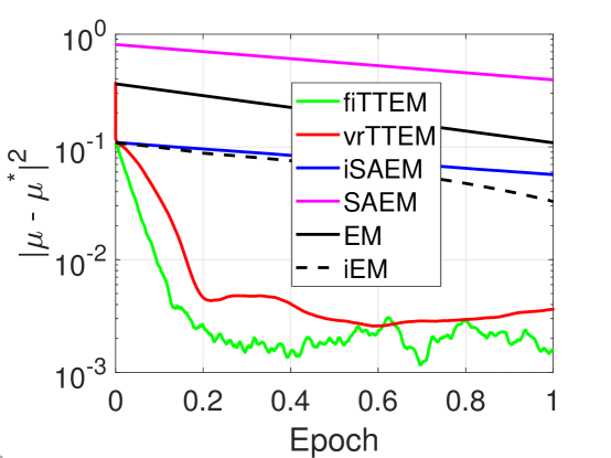
Figure 1: Precision $|\mu^{(k)}-\mu^{*}|^{2}$ for our methods (fiTTEM in green,vrTTEM in black and iSAEM in red) versus deterministic baselines (EM in dashed blue line, iEM in solid blue line) or stochastic baseline (SAEM in solid red line) against epochs elapsed. Our two variance reduced methods, i.e., fiTTEM and vrTTEM are reaching the highest accuracy.

We run the EM method until convergence (to double precision) to obtain the ML estimate $\mu^{\star}$ averaged on $50$ datasets. We compare the EM, iEM (incremental EM), SAEM, iSAEM, vrTTEM and fiTTEM methods in terms of their precision measured by $|\mu-\mu^{\star}|^{2}$. We set the stepsize of the SA-step for all method as $\gamma_{k}=1/k^{\alpha}$ with $\alpha=0.5$, and the stepsize $\rho_{k}$ for the vrTTEM and the fiTTEM to a constant stepsize equal to $1/n^{2/3}$. The number of MC samples is fixed to $M=10$. Figure 1 shows the precision $|\mu-\mu^{*}|^{2}$ for the different methods through the epoch(s) (one epoch equals $n$ iterations). The vrTTEM and fiTTEM methods outperform the other stochastic methods, supporting the benefits of our scheme.

Model Assumptions: We use the GMM example to illustrate the required assumptions. Many practical models can satisfy the compactness of the sets as in assumption A1. For instance, the GMM example satisfies the conditions in A1 as the sufficient statistics are composed of indicator functions and observations as defined in (23). Assumptions A2 and A3 are standard for the curved exponential family models. For GMM, the following (strongly convex) regularization $\operatorname{r}({\bm{\theta}})$ ensures A3:

$$\operatorname{r}({\bm{\theta}})=\frac{\delta}{2}\sum_{m=1}^{M}\mu_{m}^{2}-\epsilon\sum_{m=1}^{M}\log(\omega_{m})-\epsilon\log(1-\sum_{m=1}^{M-1}\omega_{m})\;,$$

since it ensures ${\bm{\theta}}^{(k)}$ is unique and lies in ${\rm int}(\Delta^{M})\times\mathbb{R}^{M}$. We remark that for A2, it is possible to define the Lipschitz constant $\operatorname{L}_{p}$ independently for each data $y_{i}$ to yield a refined characterization. Again, A4 is satisfied by practical models. For GMM, it can be verified by deriving the closed form expression for $\operatorname{B}({\mathbf{s}})$ and using A1. Under A1 and A3, we have $\|\hat{\bm{s}}^{(k)}\|<\infty$ since $\mathsf{S}$ is compact and $\hat{{\bm{\theta}}}^{(k)}\in{\rm int}(\Theta)$ for any $k\geq 0$ which thus ensure that the EM methods operate in a closed set throughout the optimization.

Algorithms updates: In the sequel, recall that, for all $i\in[n]$ and iteration $k$, the computed statistic $\tilde{S}_{i_{k}}^{(k)}$ is defined by (25). At iteration $k$, the several E-steps defined by (1) or (2) and (3) leads to the definition of the quantity $\hat{{\mathbf{s}}}^{(k+1)}$. Define the exact conditional expected value $\mathbb{E}_{{\bm{\theta}}}[1_{\{z_{i}=m\}}|y=y_{i}]$ as follows:

$$\widetilde{\omega}_{m}(y_{i};{\bm{\theta}})\mathrel{\mathop{:}}=\mathbb{E}_{{\bm{\theta}}}[1_{\{z_{i}=m\}}|y=y_{i}]=\frac{{\omega}_{m}\!~{}{\rm exp}(-\frac{1}{2}(y_{i}-{\mu}_{i})^{2})}{\sum_{j=1}^{M}{{\omega}_{j}\!~{}\exp(-\frac{1}{2}(y_{i}-{\mu}_{j})^{2})}}\;.$$

Then, for the GMM example, after the initialization of the quantity $\hat{{\mathbf{s}}}^{(0)}=n^{-1}\sum\nolimits_{i=1}^{n}\overline{{\mathbf{s}}}_{i}^{(0)}$, the E-step explicit updates are listed Table 2.

Table 2 Algorithms Updates for GMM

1:  Batch EM (EM)      for all $i\in[n]$, compute $\overline{{\mathbf{s}}}_{i}^{(k)}$ and set $\hat{{\mathbf{s}}}^{(k+1)}=n^{-1}\sum\nolimits_{i=1}^{n}\overline{{\mathbf{s}}}_{i}^{(k)}$

2:  Incremental EM (iEM)      draw $i_{k}$ uniformly at random on $[n]$, compute $\overline{{\mathbf{s}}}_{i_{k}}^{(k)}$ and set $\hat{{\mathbf{s}}}^{(k+1)}=n^{-1}\sum\nolimits_{i=1}^{n}\overline{{\mathbf{s}}}_{i}^{(k)}$

3:  Batch SAEM (SAEM)      for all $i\in[n]$ compute $\tilde{S}_{i}^{(k)}$ (25) and set $\hat{{\mathbf{s}}}^{(k+1)}=\hat{{\mathbf{s}}}^{(k)}(1-\gamma_{k+1})+\gamma_{k+1}S_{\textrm{tts}}^{(k)}$

4:  Variance Reduced Two-Timescale EM (vrTTEM)      draw $i_{k}$ uniformly at random on $[n]$, compute $\tilde{S}_{i_{k}}^{(k)}$ via (25) and set $\hat{{\mathbf{s}}}^{(k+1)}=\hat{{\mathbf{s}}}^{(k)}(1-\gamma_{k+1})+\gamma_{k+1}(S_{\textrm{tts}}^{(k)}(1-\rho)+\rho(\tilde{S}^{(\ell(k))}+(\tilde{S}_{i_{k}}^{(k)}-\tilde{S}_{i_{k}}^{(\ell(k))})))$

5:  Fast Incremental Two-Timescale EM (fiTTEM)      draw $i_{k}$ uniformly at random on $[n]$, compute $\tilde{S}_{i_{k}}^{(k)}$ via (25) and set $\hat{{\mathbf{s}}}^{(k+1)}=\hat{{\mathbf{s}}}^{(k)}(1-\gamma_{k+1})+\gamma_{k+1}(S_{\textrm{tts}}^{(k)}(1-\rho)+\rho(\overline{{\bm{\mathcal{S}}}}^{(k)}+(\tilde{S}_{i_{k}}^{(k)}-\tilde{S}_{i_{k}}^{(t_{i_{k}}^{k})}))\;.$

Finally, the $k$-th update reads $\hat{{\bm{\theta}}}^{(k+1)}=\overline{{\bm{\theta}}}(\hat{{\mathbf{s}}}^{(k+1)})$ where the function ${\bm{s}}\to\overline{{\bm{\theta}}}({\bm{s}})$ is defined by (27).

5.2 Deformable Template Model for Image Analysis

Model and EM Updates: Let $(y_{i},i\in[n])$ be observed gray level images defined on a grid of pixels. Let $u\in\mathcal{U}\subset\mathbb{R}^{2}$ denote the pixel index on the image and $x_{u}\in\mathcal{D}\subset\mathbb{R}^{2}$ its location. The model used in this experiment suggests that each image $y_{i}$ is a deformation of a template, noted $I:\mathcal{D}\to\mathbb{R}$, common to all images of the dataset:

$$y_{i}(u)=I\left(x_{u}-\Phi_{i}\left(x_{u},z_{i}\right)\right)+\varepsilon_{i}(u)\;,$$ (28)

where $\Phi_{i}:\mathbb{R}^{2}\to\mathbb{R}^{2}$ is a deformation function, $z_{i}$ some latent variable parameterizing this deformation and $\varepsilon_{i}\sim\mathcal{N}(0,\sigma^{2})$ is an observation error. The template model, given $\{p_{k}\}_{k=1}^{k_{p}}$ landmarks on the template, a fixed known kernel $\mathbf{K}_{\mathbf{p}}$ and a vector of parameters $\beta\in\mathbb{R}^{k_{p}}$ is defined as follows:

$$I_{\xi}=\mathbf{K}_{\mathbf{p}}\beta,\quad\textrm{where}\quad\left(\mathbf{K}_{\mathbf{p}}\beta\right)(x)=\sum_{k=1}^{k_{p}}\mathbf{K}_{\mathbf{p}}\left(x,p_{k}\right)\beta_{k}\;.$$

Given a set of landmarks $\{g_{k}\}_{k=1}^{k_{g}}$ and a fixed kernel $\mathbf{K}_{\mathbf{g}}$, we parameterize the deformation $\Phi_{i}$ as:

$$\begin{split}\Phi_{i}=\mathbf{K}_{\mathbf{g}}z_{i}\quad\textrm{where}\quad\left(\mathbf{K}_{\mathbf{g}}z_{i}\right)(x)=\sum_{k=1}^{k_{s}}\mathbf{K}_{\mathbf{g}}\left(x,g_{k}\right)\left(z_{i}^{(1)}(k),z_{i}^{(2)}(k)\right)\;,\end{split}$$

where we put a Gaussian prior on the latent variables, $z_{i}\sim\mathcal{N}(0,\Gamma)$ and $z_{i}\in\left(\mathbb{R}^{k_{g}}\right)^{2}$. Hence, the vector of parameters we want to estimate is ${\bm{\theta}}=(\beta,\Gamma,\sigma)$.

The complete model belongs to the curved exponential family, see Allassonnière et al. (2007), and its vector of sufficient statistics, noted $S=(S_{1}(z),S_{2}(z),S_{3}(z))$, reads:

$$S_{1}(z)=\frac{1}{n}\sum_{i=1}^{n}\left(\mathbf{K}_{p}^{z_{i}}\right)^{\top}y_{i},\quad S_{2}(z)=\frac{1}{n}\sum_{i=1}^{n}\left(\mathbf{K}_{p}^{z_{i}}\right)^{\top}\left(\mathbf{K}_{p}^{z_{i}}\right),\quad S_{3}(z)=\frac{1}{n}\sum_{i=1}^{n}z_{i}^{t}z_{i}\;,$$ (29)

where for any pixel $u\in\mathbb{R}^{2}$ and $j\in[k_{g}]$ we denote:

$$\mathbf{K}_{p}^{z_{i}}(x_{u},j)=\mathbf{K}_{p}^{z_{i}}(x_{u}-\phi_{i}(x_{u},z_{i}),p_{j})\;.$$

Finally, the Two-Timescale M-step yields the following parameter updates:

$$\bar{{\bm{\theta}}}(\hat{s})=\left(\begin{array}[]{c}\beta(\hat{s})=\hat{s}_{2}^{-1}(z)\hat{s}_{1}(z)\\ \Gamma(\hat{s})=\frac{1}{n}\hat{s}_{3}(z)\\ \sigma(\hat{s})=\beta(\hat{s})^{\top}\hat{s}_{2}(z)\beta(\hat{s})-2\beta(\hat{s})\hat{s}_{1}(z)\end{array}\right)\;,$$

where $\hat{s}=(\hat{s}_{1}(z),\hat{s}_{2}(z),\hat{s}_{3}(z))$ is the vector of statistics obtained via the SA-step (8) and using the MC approximation of the sufficient statistics $(S_{1}(z),S_{2}(z),S_{3}(z))$ defined in (29).

Figure 2: Training set of the USPS database (20 images for digit $5$). The variability within a class in the dataset we consider for this experiment is exhibited here. We can observe that all the images present particular features both in terms of sharpness and shape.

Numerical Experiment on the U.S. Postal Service database: We apply model (28) and Algorithm 1 to the US postal database (Hull, 1994), a collection of handwritten digits featuring $n=1\,000$, $(16\times 16)$-pixel images for each class of digits from $0$ to $9$. The main challenge with this dataset stems from the geometric dispersion within each class of digit as shown Figure 2 for digit $5$. Hence, we ought to use our deformable template model (28) in order to account for both sources of variability, i.e., the intrinsic template of each class of digit and the small and local deformations in each observed image.

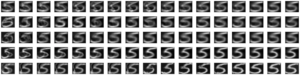
Figure 3: (USPS Digits) Estimation of the template. From top to bottom: batch, online, iSAEM, vrTTEM and fiTTEM through 7 epochs. Batch method templates are replicated in-between epochs for a fair comparison with incremental variants.

Figure 3 shows the resulting synthetic images for digit $5$ through several epochs, for the batch method, the online SAEM, the incremental SAEM and the various two-timescale methods. For all methods, the initialization of the template (5.2) is the mean of the gray level images. In our experiments, we have chosen Gaussian kernels for both, $\mathbf{K}_{\mathbf{p}}$ and $\mathbf{K}_{\mathbf{g}}$, defined on $\mathbb{R}^{2}$ and centered on the landmark points$\{p_{k}\}_{k=1}^{k_{p}}$ and $\{g_{k}\}_{k=1}^{k_{g}}$ with standard respective standard deviations of $0.12$ and $0.3$. We set $k_{p}=15$ and $k_{g}=6$ equidistributed landmarks points on the grid for the training procedure.

The hyperparameters are kept the same and are set as $M=400$, $\gamma_{k}=1/k^{0.6}$ and $p=16$. The standard deviation of the measurement errors is set to $0.1$. Those hyperparameters are inspired by relevant studies (Allassonnière et al., 2010, 2013). For the sampling phase of our methods, we use the Carlin and Chib MCMC procedure, see Carlin and Chib (1995), refer to Maire et al. (2017) for more details.

In particular, the choice of the geometric covariance, indexed by $g$, in our study is critical since it has a direct impact on the sharpness of the templates. As for the photometric hyperparameter, indexed by $p$, both the template and the geometry are impacted, in the sense that with a large photometric variance, the kernel centered on one landmark spreads out to many of its neighbors.

As the iterations proceed, the templates become progressively sharper. Figure 3 displays the virtue of the vrTTEM and fiTTEM methods leading to a more contrasted and accurate template estimate. The incremental and online versions are better in the very first epochs compared to the batch method, given the high computational cost of the latter. After a few epochs, the batch SAEM estimates similar template as the incremental and online methods due to their high variance. Our variance reduced and fast incremental variants are effective in the long run and sharpen the template estimates contrasting between the background and the regions of interest in the image.

5.3 Pharmacokinetics (PK) Model with Absorption Lag Time

The following numerical example deals characterizes the pharmacokinetics (PK) of orally administered drug to simulated patients, using a population approach, i.e., the training set consists of numerous drug plasmatic concentration per patient of the cohort. Specifically, $M=50$ synthetic datasets were generated for $n=5000$ patients with $10$ observations (concentration measures) per patient. The goal is to model the evolution of the concentration of the absorbed drug using a nonlinear and latent variable model. We consider a one-compartment PK model for oral administration with an absorption lag-time ($T^{\textrm{lag}}$), assuming first-order absorption and linear elimination processes.

Model and Explicit Updates: The final model includes the following variables: $ka$ the absorption rate constant, $V$ the volume of distribution, $k$ the elimination rate constant and $T^{\textrm{lag}}$ the absorption lag-time. We also add several covariates to our model such as $D$ the dose of drug administered, $t$ the time at which measures are taken and the weight of the patient influencing the volume $V$. More precisely, the log-volume $\log(V)$ is a linear function of the log-weight $lw70=\log(wt/70)$. Let $z_{i}=(T_{i}^{\textrm{lag}},ka_{i},V_{i},k_{i})$ be the vector of individual PK parameters, different for each individual $i$. The final model reads:

$$\begin{split}y_{ij}=f(t_{ij},z_{i})+\varepsilon_{ij}\quad\textrm{where}\quad f(t_{ij},z_{i})=\frac{D\,ka_{i}}{V(ka_{i}-k_{i})}(\operatorname{e}^{-ka_{i}\,(t_{ij}-T_{i}^{\textrm{lag}})}-\operatorname{e}^{-k_{i}\,(t_{ij}-T_{i}^{\textrm{lag}})})\;,\end{split}$$ (30)

where $y_{ij}$ is the $j$-th concentration measurement of the drug of dosage $D$ injected at time $t_{ij}$ for patient $i$. We assume in this example that the residual errors $\varepsilon_{ij}$ are independent and normally distributed with mean 0 and variance $\sigma^{2}$. Lognormal distributions are used for the four PK parameters:

$$\log(T_{i}^{\textrm{lag}})\sim\mathcal{N}(\log(T^{\textrm{lag}}_{\rm pop}),\omega^{2}_{T^{\textrm{lag}}}),\quad\log(ka_{i})\sim\mathcal{N}(\log(ka_{\rm pop}),\omega^{2}_{ka})\;,$$

$$\log(V_{i})\sim\mathcal{N}(\log(V_{\rm pop}),\omega^{2}_{V}),\quad\log(k_{i})\sim\mathcal{N}(\log(k_{\rm pop}),\omega^{2}_{k})\;.$$

We note that the complete model $p(y,z)$ defined by the structural model in (30) belongs to the curved exponential family, which vector of sufficient statistics $S=(S_{1}(z),S_{2}(z),S_{3}(z))$ reads:

$$\begin{split}S_{1}(z)=\frac{1}{n}\sum_{i=1}^{n}z_{i},\quad S_{2}(z)=\frac{1}{n}\sum_{i=1}^{n}z_{i}^{\top}z_{i},\quad S_{3}(z)=\frac{1}{n}\sum_{i=1}^{n}\left(y_{i}-f(t_{i},z_{i})\right)^{2}\;,\end{split}$$ (31)

where we have noted $y_{i}$ and $t_{i}$ the vector of observations and time for each patient $i\in[n]$. At iteration $k$, and setting the number of MC samples to $1$ for the sake of clarity, the MC sampling $z_{i}^{(k)}\sim p(z_{i}|y_{i};{\bm{\theta}}^{(k)})$ is performed using a Metropolis-Hastings procedure detailed in Algorithm 2. The quantities $S_{\textrm{tts}}^{(k+1)}$ and $\hat{{\mathbf{s}}}^{(k+1)}$ are then updated according to the different methods introduced in our paper, see Table 1. Finally the maximization step yields:

$$\overline{{\bm{\theta}}}({\bm{s}})=\left(\begin{array}[]{c}\hat{{\mathbf{s}}}^{(k+1)}_{1}\\ \hat{{\mathbf{s}}}^{(k+1)}_{2}-\hat{{\mathbf{s}}}^{(k+1)}_{1}\left(\hat{{\mathbf{s}}}^{(k+1)}_{1}\right)^{\top}\vspace{.2cm}\\ \hat{{\mathbf{s}}}^{(k+1)}_{3}\end{array}\right)=\left(\begin{array}[]{c}\overline{\bm{z_{\rm pop}}}(\hat{{\mathbf{s}}}^{(k+1)})\\ \overline{\bm{\omega_{z}}}(\hat{{\mathbf{s}}}^{(k+1)})\\ \overline{\bm{\sigma}}(\hat{{\mathbf{s}}}^{(k+1)})\end{array}\right)\;,$$ (32)

where $z_{\rm pop}$ denotes the vector of fixed effects $(T^{\textrm{lag}}_{\rm pop},ka_{\rm pop},V_{\rm pop},k_{\rm pop})$.

1:  Input: initialization $z_{i,0}\sim q(z_{i};{\bm{\delta}})$

2:  for $m=1,\cdots,M$ do

3:     Sample $z_{i,m}\sim q(z_{i};{\bm{\delta}})$.

4:     Sample $u\sim\mathcal{U}([0,1])$.

5:     Calculate the ratio $r=\frac{\pi(z_{i,m};{\bm{\theta}})/q(z_{i,m});{\bm{\delta}})}{\pi(z_{i,m-1};{\bm{\theta}})/q(z_{i,m-1});{\bm{\delta}})}$.

6:     if $u<r$ then accept $z_{i,m}$ else $z_{i,m}\leftarrow z_{i,m-1}$

7:  end for

8:  Output: $z_{i,M}$

Algorithm 2 Metropolis-Hastings algorithm

Monte Carlo study: We conduct a Monte Carlo study to showcase the benefits of our scheme. $M=50$ datasets have been simulated using the following PK parameters values: $T^{\textrm{lag}}_{\rm pop}=1$, $ka_{\rm pop}=1$, $V_{\rm pop}=8$, $k_{\rm pop}=0.1$, $\omega_{T^{\textrm{lag}}}=0.4$, $\omega_{ka}=0.5$, $\omega_{V}=0.2$, $\omega_{k}=0.3$ and $\sigma^{2}=0.5$. We define the mean square distance over the $M$ replicates as $E_{k}(\ell)=\frac{1}{M}\sum_{m=1}^{M}{\left({\bm{\theta}}_{k}^{(m)}(\ell)-{\bm{\theta}}^{*}\right)^{2}}$, and plot it against the epochs (passes over the data) in Figure 4. Note that the MC-step (6) is performed using a Metropolis-Hastings procedure since the posterior distribution under the model ${\bm{\theta}}$ noted $p(z_{i}|y_{i};{\bm{\theta}})$ is intractable, mainly due to the nonlinearity of the model (30). The Metropolis-Hastings (MH) algorithm (Meyn and Tweedie, 2012) leverages a proposal distribution $q(z_{i},\delta)$ where ${\bm{\theta}}=(z_{\rm pop},\omega_{z})$ and $\delta$ is the vector of parameters of the proposal distribution. Generally, and for simplicity, a Gaussian proposal is used. The MH algorithm employed to sample from each individual posterior distribution $\left(p(z_{i}|y_{i};{\bm{\theta}}),i\in[n]\right)$ is summarized in Algorithm 2.

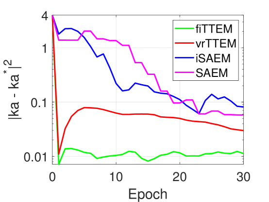
Figure 4: Mean square errors $|ka^{(k)}-ka^{*}|^{2}$ for our methods (fiTTEM in green,vrTTEM in black and iSAEM in blue) versus the SAEM baseline in red, against epochs elapsed. The errors have been averaged over $M=50$ synthetic datasets for robustness. The fiTTEM appears to be the best method among the four. The other variance reduced TTSEM method, namely vrTTEM  is quickly reaching a similar accuracy but exhibits overfitting rather quickly. The two other plain SAEM methods are the slowest.

Figure 4 shows clear advantage of variance reduced methods (vrTTEM and fiTTEM) avoiding the twists and turns displayed by the incremental and the batch methods (iSAEM and SAEM). Both our newly proposed EM methods quickly reaches a neighborhood of the solution while baselines slowly converge to it empirically stressing on the benefits of our two-timescale methods that not only temper the noise of the incremental update but also reduce the MC noise stemming from a required approximation of the expectations.

6 Conclusion

In this paper we have introduced a new class of two-timescale EM methods for learning latent variable models. In particular, the models dealt with in this paper belong to the curved exponential family and are possibly nonconvex. The nonconvexity of the problem is tackled using a Robbins-Monro type of update, which represents the first level of our class of methods. The scalability with the number of samples is performed through a variance reduced and incremental update, the second and last level of the scheme we introduce in this paper. The various algorithms are interpreted as scaled gradient methods, in the space of the sufficient statistics, and our convergence results are global, in the sense of independence of the initial values, and non-asymptotic, i.e., true for any termination iteration index. We singularly deal with the Monte Carlo noise introduced by the stochastic approximation in order to derive those convergence bounds. We empirically and theoretically show that variance reduction techniques applied to Stochastic EM type of algorithms lead to a faster convergence of the optimization phase. A panoply of numerical examples, carried out in various latent variable models, illustrate the benefits of our scheme on synthetic and real datasets. In particular, our numerical runs validate the benefits of using variance reduce variants of the SAEM over standard incremental baselines.

Appendix A Proofs for the iSAEM Algorithm

A.1 Proof of Lemma 2

Lemma.

Assume A3, A4. For all ${\mathbf{s}}\in\mathsf{S}$,

$$\upsilon_{\min}^{-1}\big{\langle}{\nabla}V({{\mathbf{s}}})\,,\,{{\mathbf{s}}}-\overline{\bm{s}}(\overline{{\bm{\theta}}}({{\mathbf{s}}}))\big{\rangle}\geq\|{{\mathbf{s}}}-\overline{\bm{s}}(\overline{{\bm{\theta}}}({{\mathbf{s}}}))\|^{2}\geq\upsilon_{\max}^{-2}\|{\nabla}V({{\mathbf{s}}})\|^{2}.$$ (33)

Proof.

Using A3 and the fact that we can exchange integration with differentiation and the Fisher’s identity, we obtain

$$\begin{split}{\nabla}_{{\mathbf{s}}}V({{\mathbf{s}}})&=\operatorname{J}_{\overline{{\bm{\theta}}}}^{{\mathbf{s}}}({\mathbf{s}})^{\top}({\nabla}_{\bm{\theta}}\operatorname{r}(\overline{{\bm{\theta}}}({{\mathbf{s}}}))+{\nabla}_{\bm{\theta}}{\textsf{L}}(\overline{\bm{\theta}}({{\mathbf{s}}})))\\ &=\operatorname{J}_{\overline{{\bm{\theta}}}}^{{\mathbf{s}}}({\mathbf{s}})^{\top}({\nabla}_{\bm{\theta}}\psi(\overline{{\bm{\theta}}}({{\mathbf{s}}}))+{\nabla}_{\bm{\theta}}\operatorname{r}(\overline{{\bm{\theta}}}({{\mathbf{s}}}))-\operatorname{J}_{\phi}^{{\bm{\theta}}}(\overline{{\bm{\theta}}}({{\mathbf{s}}}))^{\top}\overline{\bm{s}}(\overline{{\bm{\theta}}}({{\mathbf{s}}})))\\ &=\operatorname{J}_{\overline{{\bm{\theta}}}}^{{\mathbf{s}}}({\mathbf{s}})^{\top}\operatorname{J}_{\phi}^{{\bm{\theta}}}(\overline{{\bm{\theta}}}({{\mathbf{s}}}))^{\top}\!~{}({{\mathbf{s}}}-\overline{\bm{s}}(\overline{{\bm{\theta}}}({{\mathbf{s}}})))\;.\end{split}$$ (34)

Consider the following vector map:

$${{\mathbf{s}}}\to{\nabla}_{{\bm{\theta}}}L({\mathbf{s}};{\bm{\theta}})|_{{\bm{\theta}}=\overline{{\bm{\theta}}}({{\mathbf{s}}})}={\nabla}_{\bm{\theta}}\psi(\overline{{\bm{\theta}}}({{\mathbf{s}}}))+{\nabla}_{{\bm{\theta}}}\operatorname{r}(\overline{{\bm{\theta}}}({{\mathbf{s}}}))-\operatorname{J}_{\phi}^{{\bm{\theta}}}(\overline{{\bm{\theta}}}({{\mathbf{s}}}))^{\top}\!~{}{{\mathbf{s}}}\;.$$

Taking the gradient of the above map w.r.t. ${{\mathbf{s}}}$ and using assumption A3, we show that:

$${\bm{0}}=-\operatorname{J}_{\phi}^{{\bm{\theta}}}(\overline{{\bm{\theta}}}({{\mathbf{s}}}))+(\underbrace{{\nabla}_{{\bm{\theta}}}^{2}(\psi({\bm{\theta}})+\operatorname{r}({\bm{\theta}})-\big{\langle}\phi({\bm{\theta}})\,,\,{{\mathbf{s}}}\big{\rangle})}_{=\operatorname{H}_{{L}}^{{\bm{\theta}}}({{\mathbf{s}}};{\bm{\theta}})}\big{|}_{{\bm{\theta}}=\overline{{\bm{\theta}}}({{\mathbf{s}}})})\operatorname{J}_{\overline{{\bm{\theta}}}}^{{\mathbf{s}}}({\mathbf{s}})\;.$$

The above yields

$${\nabla}_{{\mathbf{s}}}V({{\mathbf{s}}})=\operatorname{B}({\mathbf{s}})({{\mathbf{s}}}-\overline{\bm{s}}(\overline{{\bm{\theta}}}({{\mathbf{s}}})))\;,$$

where we recall $\operatorname{B}({\mathbf{s}})=\operatorname{J}_{\phi}^{{\bm{\theta}}}(\overline{{\bm{\theta}}}({{\mathbf{s}}}))(\operatorname{H}_{{L}}^{{\bm{\theta}}}({{\mathbf{s}}};\overline{{\bm{\theta}}}({{\mathbf{s}}})))^{-1}\operatorname{J}_{\phi}^{{\bm{\theta}}}(\overline{{\bm{\theta}}}({{\mathbf{s}}}))^{\top}$. The proof of (33) follows directly from the assumption A4. ∎

A.2 Proof of Theorem 1

Beforehand, We present two intermediary Lemmas important for the analysis of the incremental update of the iSAEM algorithm. The first one gives a characterization of the quantity $\mathbb{E}[S_{\textrm{tts}}^{(k+1)}-\hat{{\mathbf{s}}}^{(k)}]$:

Lemma.

Assume A1. The update (1) is equivalent to the following update on the resulting statistics

$$\hat{{\mathbf{s}}}^{(k+1)}=\hat{{\mathbf{s}}}^{(k)}+\gamma_{k+1}(S_{\textrm{tts}}^{(k+1)}-\hat{{\mathbf{s}}}^{(k)})\;.$$

Also:

$$\mathbb{E}[S_{\textrm{tts}}^{(k+1)}-\hat{{\mathbf{s}}}^{(k)}]=\mathbb{E}[\overline{{\mathbf{s}}}^{(k)}-\hat{{\mathbf{s}}}^{(k)}]+(1-1/n)\mathbb{E}[\frac{1}{n}\sum_{i=1}^{n}\tilde{S}_{i}^{(\tau_{i}^{k})}-\overline{{\mathbf{s}}}^{(k)}]+\frac{1}{n}\mathbb{E}[\eta_{i_{k}}^{(k+1)}]\;,$$

where $\overline{{\mathbf{s}}}^{(k)}$ is defined by (4) and $\tau_{i}^{k}=\max\{k^{\prime}:i_{k^{\prime}}=i,~{}k^{\prime}<k\}$.

Proof.

From update (1), we have:

$$\begin{split}S_{\textrm{tts}}^{(k+1)}-\hat{{\mathbf{s}}}^{(k)}&=S_{\textrm{tts}}^{(k)}-\hat{{\mathbf{s}}}^{(k)}+\frac{1}{n}(\tilde{S}_{i_{k}}^{(k+1)}-\tilde{S}_{i_{k}}^{(\tau_{i}^{k})})\\ &=\overline{{\mathbf{s}}}^{(k)}-\hat{{\mathbf{s}}}^{(k)}+S_{\textrm{tts}}^{(k)}-\overline{{\mathbf{s}}}^{(k)}-\frac{1}{n}(\tilde{S}_{i_{k}}^{(\tau_{i}^{k})}-\tilde{S}_{i_{k}}^{(k+1)})\;.\end{split}$$

Since $\tilde{S}_{i_{k}}^{(k+1)}=\overline{{\mathbf{s}}}_{i_{k}}({\bm{\theta}}^{(k)})+\eta_{i_{k}}^{(k+1)}$ we have

$$\begin{split}S_{\textrm{tts}}^{(k+1)}-\hat{{\mathbf{s}}}^{(k)}=\overline{{\mathbf{s}}}^{(k)}-\hat{{\mathbf{s}}}^{(k)}+S_{\textrm{tts}}^{(k)}-\overline{{\mathbf{s}}}^{(k)}-\frac{1}{n}(\tilde{S}_{i_{k}}^{(\tau_{i}^{k})}-\overline{{\mathbf{s}}}_{i_{k}}({\bm{\theta}}^{(k)}))+\frac{1}{n}\eta_{i_{k}}^{(k+1)}\;.\end{split}$$

Taking the full expectation of both side of the equation leads to:

$$\begin{split}\mathbb{E}[S_{\textrm{tts}}^{(k+1)}-\hat{{\mathbf{s}}}^{(k)}]=\mathbb{E}[\overline{{\mathbf{s}}}^{(k)}-\hat{{\mathbf{s}}}^{(k)}]&+\mathbb{E}[\frac{1}{n}\sum_{i=1}^{n}\tilde{S}_{i}^{(\tau_{i}^{k})}-\overline{{\mathbf{s}}}^{(k)}]\\ &-\frac{1}{n}\mathbb{E}[\mathbb{E}[\tilde{S}_{i}^{(\tau_{i}^{k})}-\overline{{\mathbf{s}}}_{i_{k}}({\bm{\theta}}^{(k)})|\mathcal{F}_{k}]]+\frac{1}{n}\mathbb{E}[\eta_{i_{k}}^{(k+1)}]\;.\end{split}$$

Since we have $\mathbb{E}[\tilde{S}_{i}^{(\tau_{i}^{k})}|\mathcal{F}_{k}]=\frac{1}{n}\sum_{i=1}^{n}\tilde{S}_{i}^{(\tau_{i}^{k})}$ and $\mathbb{E}[\overline{{\mathbf{s}}}_{i_{k}}({\bm{\theta}}^{(k)})|\mathcal{F}_{k}]=\overline{{\mathbf{s}}}^{(k)}$, we conclude the proof of the Lemma. ∎

We also derive the following auxiliary Lemma which sets an upper bound for the quantity $\mathbb{E}[\|S_{\textrm{tts}}^{(k+1)}-\hat{\bm{s}}^{(k)}\|^{2}]$:

Lemma.

For any $k\geq 0$ and consider the iSAEM update in (1), it holds that

$$\begin{split}\mathbb{E}[\|S_{\textrm{tts}}^{(k+1)}-\hat{\bm{s}}^{(k)}\|^{2}]\leq 4\mathbb{E}[\|\overline{\bm{s}}^{(k)}-\hat{\bm{s}}^{(k)}\|^{2}]+\frac{2\operatorname{L}_{{\mathbf{s}}}^{2}}{n^{3}}\sum_{i=1}^{n}\mathbb{E}[\|\hat{\bm{s}}^{(k)}-\hat{\bm{s}}^{(t_{i}^{k})}\|^{2}]+2\frac{c_{\eta}}{M_{k}}+4\mathbb{E}[\|\frac{1}{n}\sum_{i=1}^{n}\tilde{S}_{i}^{(\tau_{i}^{k})}-\overline{{\mathbf{s}}}^{(k)}\|^{2}]\;.\end{split}$$

Proof.

Applying the iSAEM update yields the following inequality:

$$\begin{split}\mathbb{E}[\|S_{\textrm{tts}}^{(k+1)}-\hat{\bm{s}}^{(k)}\|^{2}]=&\mathbb{E}[\|S_{\textrm{tts}}^{(k)}-\hat{\bm{s}}^{(k)}-\frac{1}{n}(\tilde{S}^{(\tau_{i}^{k})}_{i_{k}}-\tilde{S}^{(k)}_{i_{k}})\|^{2}]\\ \leq&4\mathbb{E}[\|\frac{1}{n}\sum_{i=1}^{n}\tilde{S}_{i}^{(\tau_{i}^{k})}-\overline{{\mathbf{s}}}^{(k)}\|^{2}]+4\mathbb{E}[\|\overline{{\mathbf{s}}}^{(k)}-\hat{\bm{s}}^{(k)}\|^{2}]+\frac{2}{n^{2}}\mathbb{E}[\|\overline{\bm{s}}_{i_{k}}^{(k)}-\overline{\bm{s}}_{i_{k}}^{(t_{i_{k}}^{k})}\|^{2}]+2\frac{c_{\eta}}{M_{k}}\;.\end{split}$$

The last expectation can be further bounded by

$$\begin{split}&\frac{2}{n^{2}}\mathbb{E}[\|\overline{\bm{s}}_{i_{k}}^{(k)}-\overline{\bm{s}}_{i_{k}}^{(t_{i_{k}}^{k})}\|^{2}]=\frac{2}{n^{3}}\sum_{i=1}^{n}\mathbb{E}[\|\overline{\bm{s}}_{i}^{(k)}-\overline{\bm{s}}_{i}^{(t_{i}^{k})}\|^{2}]\overset{(a)}{\leq}\frac{2\operatorname{L}_{{\mathbf{s}}}^{2}}{n^{3}}\sum_{i=1}^{n}\mathbb{E}[\|\hat{\bm{s}}^{(k)}-\hat{\bm{s}}^{(t_{i}^{k})}\|^{2}]\;,\end{split}$$

where (a) is due to Lemma 1 and which concludes the proof of the Lemma.

∎

Theorem.

Assume A1-A5. Consider the iSAEM sequence $\{\hat{{\mathbf{s}}}^{(k)}\}_{k>0}\in\mathcal{S}$ obtained with $\rho_{k+1}=1$ for any $k\leq{K}_{m}$ where ${K}_{m}$ is a positive integer. Let $\{\gamma_{k}=1/(k^{a}\alpha c_{1}\overline{L})\}_{k>0}$, where $a\in(0,1)$, be a sequence of stepsizes, $c_{1}=\upsilon_{\min}^{-1}$, $\alpha=\max\{8,1+6\upsilon_{\min}\}$, $\overline{L}=\max\{\operatorname{L}_{{\mathbf{s}}},\operatorname{L}_{V}\}$, $\beta=c_{1}\overline{L}/n$. Then:

$$\upsilon_{\max}^{-2}\sum_{k=0}^{{K}_{m}}\tilde{\alpha}_{k}\mathbb{E}[\|{\nabla}V(\hat{\bm{s}}^{(k)})\|^{2}]\leq\mathbb{E}[V(\hat{\bm{s}}^{(0)})-V(\hat{\bm{s}}^{({K}_{m})})]+\sum_{k=0}^{{K}_{m}-1}\tilde{\Gamma}_{k}\mathbb{E}[\|\eta_{i_{k}}^{(k)}\|^{2}]\;.$$

Proof.

Under the smoothness of the Lyapunov function $V$ (cf. Lemma 1), we can write:

$$\begin{split}V(\hat{\bm{s}}^{(k+1)})&\leq V(\hat{\bm{s}}^{(k)})+\gamma_{k+1}\big{\langle}S_{\textrm{tts}}^{(k+1)}-\hat{\bm{s}}^{(k)}\,,\,{\nabla}V(\hat{\bm{s}}^{(k)})\big{\rangle}+\frac{\gamma_{k+1}^{2}\operatorname{L}_{V}}{2}\|S_{\textrm{tts}}^{(k+1)}-\hat{\bm{s}}^{(k)}\|^{2}\;.\end{split}$$

Taking the expectation on both sides yields:

$$\begin{split}\mathbb{E}[V(\hat{\bm{s}}^{(k+1)})]\leq\mathbb{E}[V(\hat{\bm{s}}^{(k)})]+\gamma_{k+1}\mathbb{E}[\big{\langle}S_{\textrm{tts}}^{(k+1)}-\hat{\bm{s}}^{(k)}\,,\,{\nabla}V(\hat{\bm{s}}^{(k)})\big{\rangle}]+\frac{\gamma_{k+1}^{2}\operatorname{L}_{V}}{2}\mathbb{E}[\|S_{\textrm{tts}}^{(k+1)}-\hat{\bm{s}}^{(k)}\|^{2}]\;.\end{split}$$

Using Lemma 4, we obtain:

$$\begin{split}&\mathbb{E}[\big{\langle}S_{\textrm{tts}}^{(k+1)}-\hat{\bm{s}}^{(k)}\,,\,{\nabla}V(\hat{\bm{s}}^{(k)})\big{\rangle}]\\ =&\mathbb{E}[\big{\langle}\overline{{\mathbf{s}}}^{(k)}-\hat{\bm{s}}^{(k)}\,,\,{\nabla}V(\hat{\bm{s}}^{(k)})\big{\rangle}]+\left(1-\frac{1}{n}\right)\mathbb{E}[\big{\langle}\frac{1}{n}\sum_{i=1}^{n}\tilde{S}_{i}^{(\tau_{i}^{k})}-\overline{{\mathbf{s}}}^{(k)}\,,\,{\nabla}V(\hat{\bm{s}}^{(k)})\big{\rangle}]\\ &+\frac{1}{n}\mathbb{E}[\big{\langle}\eta_{i_{k}}^{(k)}\,,\,{\nabla}V(\hat{\bm{s}}^{(k)})\big{\rangle}]\\ \overset{(a)}{\leq}&-\upsilon_{\min}\mathbb{E}[\|\overline{{\mathbf{s}}}^{(k)}-\hat{\bm{s}}^{(k)}\|^{2}]+\left(1-\frac{1}{n}\right)\mathbb{E}[\big{\langle}\frac{1}{n}\sum_{i=1}^{n}\tilde{S}_{i}^{(\tau_{i}^{k})}-\overline{{\mathbf{s}}}^{(k)}\,,\,{\nabla}V(\hat{\bm{s}}^{(k)})\big{\rangle}]\\ &+\frac{1}{n}\mathbb{E}[\big{\langle}\eta_{i_{k}}^{(k)}\,,\,{\nabla}V(\hat{\bm{s}}^{(k)})\big{\rangle}]\\ \overset{(b)}{\leq}&-\upsilon_{\min}\mathbb{E}[\|\overline{{\mathbf{s}}}^{(k)}-\hat{\bm{s}}^{(k)}\|^{2}]+\frac{1-\frac{1}{n}}{2\beta}\mathbb{E}[\|\frac{1}{n}\sum_{i=1}^{n}\tilde{S}_{i}^{(\tau_{i}^{k})}-\overline{{\mathbf{s}}}^{(k)}\|^{2}]\\ &+\frac{\beta(n-1)+1}{2n}\mathbb{E}[\left\|{\nabla}V(\hat{\bm{s}}^{(k)})\right\|^{2}]+\frac{1}{2n}\mathbb{E}[\|\eta_{i_{k}}^{(k)}\|^{2}]\\ \overset{(a)}{\leq}&\left(\upsilon^{2}_{\max}\frac{\beta(n-1)+1}{2n}-\upsilon_{\min}\right)\mathbb{E}[\|\overline{{\mathbf{s}}}^{(k)}-\hat{\bm{s}}^{(k)}\|^{2}]+\frac{1-\frac{1}{n}}{2\beta}\mathbb{E}[\|\frac{1}{n}\sum_{i=1}^{n}\tilde{S}_{i}^{(\tau_{i}^{k})}-\overline{{\mathbf{s}}}^{(k)}\|^{2}]\\ &+\frac{1}{2n}\mathbb{E}[\|\eta_{i_{k}}^{(k)}\|^{2}]\;,\end{split}$$

where (a) is due to the growth condition (2) and (b) is due to Young’s inequality (with $\beta\to 1$). Note $a_{k}=\gamma_{k+1}\left(\upsilon_{\min}-\upsilon^{2}_{\max}\frac{\beta(n-1)+1}{2n}\right)$ and

$$\begin{split}a_{k}\mathbb{E}[\|\overline{{\mathbf{s}}}^{(k)}-\hat{\bm{s}}^{(k)}\|^{2}]\leq&\mathbb{E}[V(\hat{\bm{s}}^{(k)})-V(\hat{\bm{s}}^{(k+1)})]+\frac{\gamma_{k+1}^{2}\operatorname{L}_{V}}{2}\mathbb{E}[\|S_{\textrm{tts}}^{(k+1)}-\hat{\bm{s}}^{(k)}\|^{2}]\\ &+\frac{\gamma_{k+1}(1-\frac{1}{n})}{2\beta}\mathbb{E}[\|\frac{1}{n}\sum_{i=1}^{n}\tilde{S}_{i}^{(\tau_{i}^{k})}-\overline{{\mathbf{s}}}^{(k)}\|^{2}]+\frac{\gamma_{k+1}}{2n}\mathbb{E}[\|\eta_{i_{k}}^{(k)}\|^{2}]\;.\end{split}$$ (35)

We now give an upper bound of $\mathbb{E}[\|S_{\textrm{tts}}^{(k+1)}-\hat{\bm{s}}^{(k)}\|^{2}]$ using Lemma 5 and plug it into (35):

$$\begin{split}(a_{k}-2\gamma_{k+1}^{2}\operatorname{L}_{V})\mathbb{E}[\|\overline{{\mathbf{s}}}^{(k)}-\hat{\bm{s}}^{(k)}\|^{2}]\leq&\mathbb{E}[V(\hat{\bm{s}}^{(k)})-V(\hat{\bm{s}}^{(k+1)})]\\ &+\gamma_{k+1}\left(\frac{1}{2\beta}(1-1/n)+2\gamma_{k+1}\operatorname{L}_{V}\right)\mathbb{E}[\|\frac{1}{n}\sum_{i=1}^{n}\tilde{S}_{i}^{(\tau_{i}^{k})}-\overline{{\mathbf{s}}}^{(k)}\|^{2}]\\ &+\gamma_{k+1}\left(\gamma_{k+1}\operatorname{L}_{V}+\frac{1}{2n}\right)\mathbb{E}[\|\eta_{i_{k}}^{(k)}\|^{2}]\\ &+\frac{\gamma_{k+1}^{2}\operatorname{L}_{V}\operatorname{L}_{{\mathbf{s}}}^{2}}{n^{3}}\sum_{i=1}^{n}\mathbb{E}[\|\hat{\bm{s}}^{(k)}-\hat{\bm{s}}^{(\tau_{i}^{k})}\|^{2}]\;.\end{split}$$ (36)

Next, we observe that

$$\frac{1}{n}\sum_{i=1}^{n}\mathbb{E}[\|\hat{\bm{s}}^{(k+1)}-\hat{\bm{s}}^{(t_{i}^{k+1})}\|^{2}]=\frac{1}{n}\sum_{i=1}^{n}(\frac{1}{n}\mathbb{E}[\|\hat{\bm{s}}^{(k+1)}-\hat{\bm{s}}^{(k)}\|^{2}]+\frac{n-1}{n}\mathbb{E}[\|\hat{\bm{s}}^{(k+1)}-\hat{\bm{s}}^{(\tau_{i}^{k})}\|^{2}])\;,$$

where the equality holds as $i_{k}$ and $j_{k}$ are drawn independently. For any $\beta>0$, it holds

$$\begin{split}&\mathbb{E}[\|\hat{\bm{s}}^{(k+1)}-\hat{\bm{s}}^{(t_{i}^{k})}\|^{2}]\\ =&\mathbb{E}[\|\hat{\bm{s}}^{(k+1)}-\hat{\bm{s}}^{(k)}\|^{2}+\|\hat{\bm{s}}^{(k)}-\hat{\bm{s}}^{(\tau_{i}^{k})}\|^{2}+2\big{\langle}\hat{\bm{s}}^{(k+1)}-\hat{\bm{s}}^{(k)}\,,\,\hat{\bm{s}}^{(k)}-\hat{\bm{s}}^{(\tau_{i}^{k})}\big{\rangle}]\\ =&\mathbb{E}[\|\hat{\bm{s}}^{(k+1)}-\hat{\bm{s}}^{(k)}\|^{2}+\|\hat{\bm{s}}^{(k)}-\hat{\bm{s}}^{(\tau_{i}^{k})}\|^{2}-2\gamma_{k+1}\big{\langle}\hat{\bm{s}}^{(k)}-S_{\textrm{tts}}^{(k+1)}\,,\,\hat{\bm{s}}^{(k)}-\hat{\bm{s}}^{(\tau_{i}^{k})}\big{\rangle}]\\ \leq&\mathbb{E}[\|\hat{\bm{s}}^{(k+1)}-\hat{\bm{s}}^{(k)}\|^{2}+\|\hat{\bm{s}}^{(k)}-\hat{\bm{s}}^{(\tau_{i}^{k})}\|^{2}+\frac{\gamma_{k+1}}{\beta}\|\hat{\bm{s}}^{(k)}-S_{\textrm{tts}}^{(k+1)}\|^{2}\\ &+\gamma_{k+1}\beta\|\hat{\bm{s}}^{(k)}-\hat{\bm{s}}^{(\tau_{i}^{k})}\|^{2}]\;,\end{split}$$

where the last inequality is due to Young’s inequality. Subsequently, we have

$$\begin{split}\frac{1}{n}\sum_{i=1}^{n}\mathbb{E}[\|\hat{\bm{s}}^{(k+1)}-\hat{\bm{s}}^{(\tau_{i}^{k+1})}\|^{2}]\leq&\mathbb{E}[\|\hat{\bm{s}}^{(k+1)}-\hat{\bm{s}}^{(k)}\|^{2}]+\frac{n-1}{n^{2}}\sum_{i=1}^{n}\mathbb{E}[(1+\gamma_{k+1}\beta)\|\hat{\bm{s}}^{(k)}-\hat{\bm{s}}^{(\tau_{i}^{k})}\|^{2}\\ &+\frac{\gamma_{k+1}}{\beta}\|\hat{\bm{s}}^{(k)}-S_{\textrm{tts}}^{(k+1)}\|^{2}]\;.\end{split}$$

Observe that $\hat{\bm{s}}^{(k+1)}-\hat{\bm{s}}^{(k)}=-\gamma_{k+1}(\hat{\bm{s}}^{(k)}-S_{\textrm{tts}}^{(k+1)})$. Applying Lemma 5 yields

$$\begin{split}&\frac{1}{n}\sum_{i=1}^{n}\mathbb{E}[\|\hat{\bm{s}}^{(k+1)}-\hat{\bm{s}}^{(\tau_{i}^{k+1})}\|^{2}]\\ \leq&(\gamma_{k+1}^{2}+\frac{n-1}{n}\frac{\gamma_{k+1}}{\beta})\mathbb{E}[\|S_{\textrm{tts}}^{(k+1)}-\hat{\bm{s}}^{(k)}\|^{2}]+\sum_{i=1}^{n}\mathbb{E}[\frac{1-\frac{1}{n}+\gamma_{k+1}\beta}{n}\|\hat{\bm{s}}^{(k)}-\hat{\bm{s}}^{(\tau_{i}^{k})}\|^{2}]\\ \leq&4(\gamma_{k+1}^{2}+\frac{\gamma_{k+1}}{\beta})\mathbb{E}[\|\overline{\bm{s}}^{(k)}-\hat{\bm{s}}^{(k)}\|^{2}]+2(\gamma_{k+1}^{2}+\frac{\gamma_{k+1}}{\beta})\mathbb{E}[\|\eta_{i_{k}}^{(k)}\|^{2}]\\ +&4(\gamma_{k+1}^{2}+\frac{\gamma_{k+1}}{\beta})\mathbb{E}[\|\frac{1}{n}\sum_{i=1}^{n}\tilde{S}_{i}^{(\tau_{i}^{k})}-\overline{{\mathbf{s}}}^{(k)}\|^{2}]\\ +&\sum_{i=1}^{n}\mathbb{E}[\frac{1-\frac{1}{n}+\gamma_{k+1}\beta+\frac{2\gamma_{k+1}\operatorname{L}_{{\mathbf{s}}}^{2}}{n^{2}}(\gamma_{k+1}+\frac{1}{\beta})}{n}\|\hat{\bm{s}}^{(k)}-\hat{\bm{s}}^{(t_{i}^{k})}\|^{2}]\;.\end{split}$$

Let us define

$$\Delta^{(k)}\mathrel{\mathop{:}}=\frac{1}{n}\sum_{i=1}^{n}\mathbb{E}[\|\hat{\bm{s}}^{(k)}-\hat{\bm{s}}^{(\tau_{i}^{k})}\|^{2}]\;.$$

From the above, we obtain

$$\begin{split}\Delta^{(k+1)}&\leq(1-\frac{1}{n}+\gamma_{k+1}\beta+\frac{2\gamma_{k+1}\operatorname{L}_{{\mathbf{s}}}^{2}}{n^{2}}(\gamma_{k+1}+\frac{1}{\beta}))\Delta^{(k)}\\ &+4(\gamma_{k+1}^{2}+\frac{\gamma_{k+1}}{\beta})\mathbb{E}[\|\overline{\bm{s}}^{(k)}-\hat{\bm{s}}^{(k)}\|^{2}]+2(\gamma_{k+1}^{2}+\frac{\gamma_{k+1}}{\beta})\mathbb{E}[\|\eta_{i_{k}}^{(k)}\|^{2}]\\ &+4(\gamma_{k+1}^{2}+\frac{\gamma_{k+1}}{\beta})\mathbb{E}[\|\frac{1}{n}\sum_{i=1}^{n}\tilde{S}_{i}^{(\tau_{i}^{k})}-\overline{{\mathbf{s}}}^{(k)}\|^{2}]\;.\end{split}$$

Setting $c_{1}=\upsilon_{\min}^{-1}$, $\alpha=\max\{8,1+6\upsilon_{\min}\}$, $\overline{L}=\max\{\operatorname{L}_{{\mathbf{s}}},\operatorname{L}_{V}\}$, $\gamma_{k+1}=\frac{1}{k\alpha c_{1}\overline{L}}$, $\beta=\frac{c_{1}\overline{L}}{n}$, we remark $c_{1}(k\alpha-1)\geq c_{1}(\alpha-1)\geq 6$ and we observe that

$$1-\frac{1}{n}+\gamma_{k+1}\beta+\frac{2\gamma_{k+1}\operatorname{L}_{{\mathbf{s}}}^{2}}{n^{2}}(\gamma_{k+1}+\frac{1}{\beta})\leq 1-\frac{c_{1}(k\alpha-1)-4}{k\alpha nc_{1}}\leq 1-\frac{2}{k\alpha nc_{1}}\;,$$

which shows that $1-\frac{1}{n}+\gamma_{k+1}\beta+\frac{2\gamma_{k+1}\operatorname{L}_{{\mathbf{s}}}^{2}}{n^{2}}(\gamma_{k+1}+\frac{1}{\beta})\in(0,1)$ for any $k>0$. Denote $\Lambda_{(k+1)}=\frac{1}{n}-\gamma_{k+1}\beta-\frac{2\gamma_{k+1}\operatorname{L}_{{\mathbf{s}}}^{2}}{n^{2}}(\gamma_{k+1}+\frac{1}{\beta})$ and note that $\Delta^{(0)}=0$, thus the telescoping sum yields:

$$\begin{split}\Delta^{(k+1)}&\leq 4\sum_{\ell=0}^{k}\prod_{j=\ell+1}^{k}(1-\Lambda_{(j)})(\gamma_{\ell+1}^{2}+\frac{\gamma_{\ell+1}}{\beta})\mathbb{E}[\|\overline{\bm{s}}^{(\ell)}-\hat{\bm{s}}^{(\ell)}\|^{2}]\\ &+2\sum_{\ell=0}^{k}\prod_{j=\ell+1}^{k}(1-\Lambda_{(j)})(\gamma_{\ell+1}^{2}+\frac{\gamma_{\ell+1}}{\beta})\mathbb{E}[\|\eta_{i_{\ell}}^{(\ell)}\|^{2}]\\ &+4\sum_{\ell=0}^{k}\prod_{j=\ell+1}^{k}(1-\Lambda_{(j)})(\gamma_{\ell+1}^{2}+\frac{\gamma_{\ell+1}}{\beta})\mathbb{E}[\|\frac{1}{n}\sum_{i=1}^{n}\tilde{S}_{i}^{(\tau_{i}^{\ell})}-\overline{{\mathbf{s}}}^{(\ell)}\|^{2}]\;.\end{split}$$

Note $\omega_{k,\ell}=\prod_{j=\ell+1}^{k}(1-\Lambda_{(j)})$ Summing on both sides over $k=0$ to $k={K}_{m}-1$ yields:

$$\begin{split}&\sum_{k=0}^{{K}_{m}-1}\Delta^{(k+1)}\\ =&4\sum_{k=0}^{{K}_{m}-1}(\gamma_{k+1}^{2}+\frac{\gamma_{k+1}}{\beta})\omega_{k,1}\mathbb{E}[\|\overline{\bm{s}}^{(k)}-\hat{\bm{s}}^{(k)}\|^{2}]+2\sum_{k=0}^{{K}_{m}-1}(\gamma_{k+1}^{2}+\frac{\gamma_{k+1}}{\beta})\omega_{k,1}\mathbb{E}[\left\|\eta_{i_{\ell}}^{(k)}\right\|^{2}]\\ +&\sum_{k=0}^{{K}_{m}-1}4(\gamma_{k+1}^{2}+\frac{\gamma_{k+1}}{\beta})\omega_{k,1}\mathbb{E}[\|\frac{1}{n}\sum_{i=1}^{n}\tilde{S}_{i}^{(\tau_{i}^{k})}-\overline{{\mathbf{s}}}^{(k)}\|^{2}]\\ \leq&\sum_{k=0}^{{K}_{m}-1}\frac{4(\gamma_{k+1}^{2}+\frac{\gamma_{k+1}}{\beta})}{\Lambda_{(k+1)}}\mathbb{E}[\|\overline{\bm{s}}^{(k)}-\hat{\bm{s}}^{(k)}\|^{2}]+\sum_{k=0}^{{K}_{m}-1}\frac{2(\gamma_{k+1}^{2}+\frac{\gamma_{k+1}}{\beta})}{\Lambda_{(k+1)}}\mathbb{E}[\left\|\eta_{i_{\ell}}^{(k)}\right\|^{2}]\\ +&\sum_{k=0}^{{K}_{m}-1}\frac{4(\gamma_{k+1}^{2}+\frac{\gamma_{k+1}}{\beta})}{\Lambda_{(k+1)}}\mathbb{E}[\|\frac{1}{n}\sum_{i=1}^{n}\tilde{S}_{i}^{(\tau_{i}^{k})}-\overline{{\mathbf{s}}}^{(k)}\|^{2}]\;.\end{split}$$ (37)

We recall (36) where we have summed on both sides from $k=0$ to $k={K}_{m}-1$:

$$\begin{split}&\sum_{k=0}^{{K}_{m}-1}\left(a_{k}-2\gamma_{k+1}^{2}\operatorname{L}_{V}\right)\mathbb{E}[\|\overline{{\mathbf{s}}}^{(k)}-\hat{\bm{s}}^{(k)}\|^{2}]\\ \leq&\mathbb{E}[V(\hat{\bm{s}}^{(0)})-V(\hat{\bm{s}}^{(K)})]+\sum_{k=0}^{{K}_{m}-1}\gamma_{k+1}\left(\frac{1}{2\beta}(1-1/n)+2\gamma_{k+1}\operatorname{L}_{V}\right)\mathbb{E}[\|\frac{1}{n}\sum_{i=1}^{n}\tilde{S}_{i}^{(\tau_{i}^{k})}-\overline{{\mathbf{s}}}^{(k)}\|^{2}]\\ +&\sum_{k=0}^{{K}_{m}-1}\gamma_{k+1}\left(\gamma_{k+1}\operatorname{L}_{V}+\frac{1}{2n}\right)\mathbb{E}[\|\eta_{i_{k}}^{(k)}\|^{2}]+\sum_{k=0}^{{K}_{m}-1}\frac{\gamma_{k+1}^{2}\operatorname{L}_{V}\operatorname{L}_{{\mathbf{s}}}^{2}}{n^{2}}\Delta^{(k)}\;.\end{split}$$ (38)

Plugging (37) into (38) results in:

$$\begin{split}\sum_{k=0}^{{K}_{m}-1}\tilde{\alpha}_{k}\mathbb{E}[\|\overline{{\mathbf{s}}}^{(k)}-\hat{\bm{s}}^{(k)}\|^{2}]+\sum_{k=0}^{{K}_{m}-1}\tilde{\beta}_{k}\mathbb{E}[\|\frac{1}{n}\sum_{i=1}^{n}\tilde{S}_{i}^{(\tau_{i}^{k})}-\overline{{\mathbf{s}}}^{(k)}\|^{2}]\leq\mathbb{E}[V(\hat{\bm{s}}^{(0)})-V(\hat{\bm{s}}^{(K)})]+\sum_{k=0}^{{K}_{m}-1}\tilde{\Gamma}_{k}\mathbb{E}[\|\eta_{i_{k}}^{(k)}\|^{2}]\;,\end{split}$$

where

$$\tilde{\alpha}_{k}=a_{k}-2\gamma_{k+1}^{2}\operatorname{L}_{V}-\frac{\gamma_{k+1}^{2}\operatorname{L}_{V}\operatorname{L}_{{\mathbf{s}}}^{2}}{n^{2}}\frac{4(\gamma_{k+1}^{2}+\frac{\gamma_{k+1}}{\beta})}{\Lambda_{(k+1)}}\;,$$

$$\tilde{\beta}_{k}=\gamma_{k+1}\left(\frac{1}{2\beta}(1-1/n)+2\gamma_{k+1}\operatorname{L}_{V}\right)-\frac{\gamma_{k+1}^{2}\operatorname{L}_{V}\operatorname{L}_{{\mathbf{s}}}^{2}}{n^{2}}\frac{4(\gamma_{k+1}^{2}+\frac{\gamma_{k+1}}{\beta})}{\Lambda_{(k+1)}}\;,$$

$$\tilde{\Gamma}_{k}=\gamma_{k+1}\left(\gamma_{k+1}\operatorname{L}_{V}+\frac{1}{2n}\right)+\frac{\gamma_{k+1}^{2}\operatorname{L}_{V}\operatorname{L}_{{\mathbf{s}}}^{2}}{n^{2}}\frac{2(\gamma_{k+1}^{2}+\frac{\gamma_{k+1}}{\beta})}{\Lambda_{(k+1)}}\;,$$

and

$$a_{k}=\gamma_{k+1}\left(\upsilon_{\min}-\upsilon^{2}_{\max}\frac{\beta(n-1)+1}{2n}\right)\;,$$

$$\Lambda_{(k+1)}=\frac{1}{n}-\gamma_{k+1}\beta-\frac{2\gamma_{k+1}\operatorname{L}_{{\mathbf{s}}}^{2}}{n^{2}}(\gamma_{k+1}+\frac{1}{\beta})\;,$$

$$c_{1}=\upsilon_{\min}^{-1},\alpha=\max\{8,1+6\upsilon_{\min}\},\overline{L}=\max\{\operatorname{L}_{{\mathbf{s}}},\operatorname{L}_{V}\},\gamma_{k+1}=\frac{1}{k\alpha c_{1}\overline{L}},\beta=\frac{c_{1}\overline{L}}{n}\;.$$

When, for any $k>0$, $\tilde{\alpha}_{k}\geq 0$, we have by Lemma 2 that:

$$\sum_{k=0}^{{K}_{m}}\tilde{\alpha}_{k}\mathbb{E}[\|{\nabla}V(\hat{\bm{s}}^{(k)})\|^{2}]\leq\upsilon_{\max}^{2}\sum_{k=0}^{{K}_{m}}\tilde{\alpha}_{k}\mathbb{E}[\|\overline{{\mathbf{s}}}^{(k)}-\hat{\bm{s}}^{(k)}\|^{2}]\;,$$

concluding the proof of the Theorem. ∎

Appendix B Proofs for the vrTTEM and the fiTTEM Algorithms

B.1 Additional Intermediary Results

We introduce additional Lemmas below before getting into the proofs of the desired results.

Lemma 9.

Consider the vrTTEM update (2) with $\rho_{k}=\rho$, it holds for all $k>0$

$$\begin{split}\mathbb{E}[\|\hat{\bm{s}}^{(k)}-S_{\textrm{tts}}^{(k+1)}\|^{2}]\leq&2\rho^{2}\mathbb{E}[\|\hat{\bm{s}}^{(k)}-\overline{\bm{s}}^{(k)}\|^{2}]+2\rho^{2}\operatorname{L}_{{\mathbf{s}}}^{2}\mathbb{E}[\|\hat{\bm{s}}^{(k)}-\hat{\bm{s}}^{(\ell(k))}\|^{2}]\\ &+2(1-\rho)^{2}\mathbb{E}[\|\hat{\bm{s}}^{((k))}-S_{\textrm{tts}}^{(k)}\|^{2}]+2\rho^{2}\mathbb{E}[\|\eta_{i_{k}}^{(k+1)}\|^{2}]\;,\end{split}$$

where we recall that $\ell(k)$ is the first iteration number in the epoch that iteration $k$ is in.

Proof.

Beforehand, we provide an alternate expression of the quantity $\hat{\bm{s}}^{(k+1)}-\hat{\bm{s}}^{(k)}$ that will be useful throughout this proof:

$$\begin{split}\hat{\bm{s}}^{(k+1)}-\hat{\bm{s}}^{(k)}&=-\gamma_{k+1}(\hat{\bm{s}}^{(k)}-S_{\textrm{tts}}^{(k+1)})\\ &=-\gamma_{k+1}(\hat{\bm{s}}^{(k)}-(1-\rho)S_{\textrm{tts}}^{(k)}-\rho{\bm{\mathcal{S}}}^{(k+1)})\\ &=-\gamma_{k+1}\left((1-\rho)[\hat{\bm{s}}^{(k)}-S_{\textrm{tts}}^{(k)}]+\rho[\hat{\bm{s}}^{(k)}-{\bm{\mathcal{S}}}^{(k+1)}]\right)\;.\end{split}$$ (39)

We observe, using the identity (39), that

$$\begin{split}\mathbb{E}[\|\hat{\bm{s}}^{(k)}-S_{\textrm{tts}}^{(k+1)}\|^{2}]\leq&2\rho^{2}\mathbb{E}[\|\hat{\bm{s}}^{(k)}-\overline{\bm{s}}^{(k)}\|^{2}]+2\rho^{2}\mathbb{E}[\|\overline{\bm{s}}^{(k)}-{\bm{\mathcal{S}}}^{(k+1)}\|^{2}]\\ &+2(1-\rho)^{2}\mathbb{E}[\|\hat{\bm{s}}^{((k))}-S_{\textrm{tts}}^{(k)}\|^{2}].\end{split}$$ (40)

For the latter term, we obtain its upper bound as

$$\begin{split}\mathbb{E}[\|\overline{\bm{s}}^{(k)}-{\bm{\mathcal{S}}}^{(k+1)}\|^{2}]=&\mathbb{E}[\|\frac{1}{n}\sum_{i=1}^{n}(\overline{\bm{s}}_{i}^{(k)}-\tilde{S}_{i}^{\ell(k)})-(\overline{\bm{s}}_{i_{k}}^{(k)}-\tilde{S}_{i_{k}}^{(\ell(k))})\|^{2}]\\ \overset{(a)}{\leq}&\mathbb{E}[\|\overline{\bm{s}}_{i_{k}}^{(k)}-\overline{\bm{s}}_{i_{k}}^{(\ell(k))}\|^{2}]+\mathbb{E}[\|\eta_{i_{k}}^{(k+1)}\|^{2}]\\ &\overset{(b)}{\leq}\operatorname{L}_{{\mathbf{s}}}^{2}\mathbb{E}[\|\hat{\bm{s}}^{(k)}-\hat{\bm{s}}^{(\ell(k))}\|^{2}]+\mathbb{E}[\|\eta_{i_{k}}^{(k+1)}\|^{2}]\;,\end{split}$$

where $(a)$ uses the variance inequality and $(b)$ uses Lemma 1. Substituting into (40) proves the lemma. ∎

Lemma 10.

Consider the fiTTEM update (3) with $\rho_{k}=\rho$. It holds for all $k>0$ that

$$\begin{split}\mathbb{E}[\|\hat{\bm{s}}^{(k)}-S_{\textrm{tts}}^{(k+1)}\|^{2}]\leq&2\rho^{2}\mathbb{E}[\|\hat{\bm{s}}^{(k)}-\overline{\bm{s}}^{(k)}\|^{2}]+2\rho^{2}\frac{\operatorname{L}_{{\mathbf{s}}}^{2}}{n}\sum_{i=1}^{n}\mathbb{E}[\|\hat{\bm{s}}^{(k)}-\hat{\bm{s}}^{(t_{i}^{k})}\|^{2}]\\ &+2(1-\rho)^{2}\mathbb{E}[\|\hat{\bm{s}}^{((k))}-S_{\textrm{tts}}^{(k)}\|^{2}]+2\rho^{2}\mathbb{E}[\|\eta_{i_{k}}^{(k+1)}\|^{2}]\;,\end{split}$$

where $\operatorname{L}_{{\mathbf{s}}}$ is the smoothness constant defined in Lemma 1.

Proof.

Beforehand, we provide a rewriting of the quantity $\hat{\bm{s}}^{(k+1)}-\hat{\bm{s}}^{(k)}$ that will be useful throughout this proof:

$$\begin{split}\hat{\bm{s}}^{(k+1)}-\hat{\bm{s}}^{(k)}&=-\gamma_{k+1}(\hat{\bm{s}}^{(k)}-S_{\textrm{tts}}^{(k+1)})\\ &=-\gamma_{k+1}(\hat{\bm{s}}^{(k)}-(1-\rho)S_{\textrm{tts}}^{(k)}-\rho{\bm{\mathcal{S}}}^{(k+1)})\\ &=-\gamma_{k+1}\left((1-\rho)[\hat{\bm{s}}^{(k)}-S_{\textrm{tts}}^{(k)}]+\rho[\hat{\bm{s}}^{(k)}-{\bm{\mathcal{S}}}^{(k+1)}]\right)\\ &=-\gamma_{k+1}\left((1-\rho)[\hat{\bm{s}}^{(k)}-S_{\textrm{tts}}^{(k)}]+\rho[\hat{\bm{s}}^{(k)}-\overline{{\bm{\mathcal{S}}}}^{(k)}-(\tilde{S}_{i_{k}}^{(k)}-\tilde{S}_{i_{k}}^{(t_{i_{k}}^{k})})]\right)\;.\end{split}$$ (41)

We observe, using the identity (41), that

$$\mathbb{E}[\|\hat{\bm{s}}^{(k)}-S_{\textrm{tts}}^{(k+1)}\|^{2}]\leq 2\rho^{2}\mathbb{E}[\|\hat{\bm{s}}^{(k)}-\overline{\bm{s}}^{(k)}\|^{2}]+2\rho^{2}\mathbb{E}[\|\overline{\bm{s}}^{(k)}-{\bm{\mathcal{S}}}^{(k+1)}\|^{2}]+2(1-\rho)^{2}\mathbb{E}[\|\hat{\bm{s}}^{((k))}-S_{\textrm{tts}}^{(k)}\|^{2}]\;.$$ (42)

For the latter term, we obtain its upper bound as

$$\begin{split}\mathbb{E}[\|\overline{\bm{s}}^{(k)}-{\bm{\mathcal{S}}}^{(k+1)}\|^{2}]&=\mathbb{E}[\|\frac{1}{n}\sum_{i=1}^{n}(\overline{\bm{s}}_{i}^{(k)}-\overline{{\bm{\mathcal{S}}}}_{i}^{(k)})-(\tilde{S}_{i_{k}}^{(k)}-\tilde{S}_{i_{k}}^{(t_{i_{k}}^{k})})\|^{2}]\\ &\overset{(a)}{\leq}\mathbb{E}[\|\overline{\bm{s}}_{i_{k}}^{(k)}-\overline{\bm{s}}_{i_{k}}^{(\ell(k))}\|^{2}]+\mathbb{E}[\|\eta_{i_{k}}^{(k+1)}\|^{2}]\;,\end{split}$$

where $(a)$ uses the variance inequality. We can further bound the last expectation using Lemma 1:

$$\mathbb{E}[\|\overline{\bm{s}}_{i_{k}}^{(k)}-\overline{\bm{s}}_{i_{k}}^{(t_{i_{k}}^{k})}\|^{2}]=\frac{1}{n}\sum_{i=1}^{n}\mathbb{E}[\|\overline{\bm{s}}_{i}^{(k)}-\overline{\bm{s}}_{i}^{(t_{i}^{k})}\|^{2}]\overset{(a)}{\leq}\frac{\operatorname{L}_{{\mathbf{s}}}^{2}}{n}\sum_{i=1}^{n}\mathbb{E}[\|\hat{\bm{s}}^{(k)}-\hat{\bm{s}}^{(t_{i}^{k})}\|^{2}]\;.$$

Substituting the above into (42) proves the lemma. ∎

Lemma 11.

Considering a decreasing stepsize $\gamma_{k}\in(0,1)$ and a constant $\rho\in(0,1)$, we have

$$\begin{split}\mathbb{E}[\|\hat{\bm{s}}^{(k)}-S_{\textrm{tts}}^{(k)}\|^{2}]\leq\frac{\rho}{1-\rho}\sum_{\ell=0}^{k}(1-\gamma_{\ell})^{2}({\bm{\mathcal{S}}}^{(\ell)}-\tilde{S}^{(\ell)})\;,\end{split}$$

where ${\bm{\mathcal{S}}}^{(k)}$ is defined either by Line 2 (vrTTEM) or Line 3 (fiTTEM).

Proof.

We begin by writing the two-timescale update:

$$\begin{split}&S_{\textrm{tts}}^{(k+1)}=S_{\textrm{tts}}^{(k)}+\rho({\bm{\mathcal{S}}}^{(k+1)}-S_{\textrm{tts}}^{(k)})\;,\\ &\hat{{\mathbf{s}}}^{(k+1)}=\hat{{\mathbf{s}}}^{(k)}+\gamma_{k+1}(S_{\textrm{tts}}^{(k+1)}-\hat{{\mathbf{s}}}^{(k)})\;,\end{split}$$ (43)

where ${\bm{\mathcal{S}}}^{(k+1)}=\frac{1}{n}\sum_{i=1}^{n}\tilde{S}_{i}^{(t_{i}^{k})}+(\tilde{S}_{i_{k}}^{(k)}-\tilde{S}_{i_{k}}^{(t_{i_{k}}^{k})})$ according to (3). Denote $\delta^{(k+1)}=\hat{\bm{s}}^{(k+1)}-S_{\textrm{tts}}^{(k+1)}$. Then from (43), doing the subtraction of both equations yields:

$$\delta^{(k+1)}=(1-\gamma_{k+1})\delta^{(k)}+\frac{\rho}{1-\rho}(1-\gamma_{k+1})({\bm{\mathcal{S}}}^{(k+1)}-S_{\textrm{tts}}^{(k+1)})\;.$$

Using the telescoping sum and noting that $\delta^{(0)}=0$, we have

$$\delta^{(k+1)}\leq\frac{\rho}{1-\rho}\sum_{\ell=0}^{k}(1-\gamma_{\ell+1})^{2}({\bm{\mathcal{S}}}^{(\ell+1)}-\tilde{S}^{(\ell+1)})\;.$$

∎

B.2 Proofs of Auxiliary Lemmas ( Lemma 6, Lemma 8 and Lemma 3)

Lemma.

At iteration $k+1$,the drift term of update (3), with $\rho_{k+1}=\rho$, is equivalent to :

$$\begin{split}\hat{\bm{s}}^{(k)}-S_{\textrm{tts}}^{(k+1)}=&\rho(\hat{\bm{s}}^{(k)}-\overline{{\mathbf{s}}}^{(k)})+\rho\eta_{i_{k}}^{(k+1)}+\rho[(\overline{{\mathbf{s}}}_{i_{k}}^{(k)}-\tilde{S}_{i_{k}}^{(t_{i_{k}}^{k})})-\mathbb{E}[\overline{{\mathbf{s}}}_{i_{k}}^{(k)}-\tilde{S}_{i_{k}}^{(t_{i_{k}}^{k})}]]\\ &+(1-\rho)\left(\hat{\bm{s}}^{(k)}-\tilde{S}^{(k)}\right)\;,\end{split}$$

where we recall that $\eta_{i_{k}}^{(k+1)}$, defined in (13), which is the gap between the MC approximation and the expected statistics.

Proof.

Using the fiTTEM update $S_{\textrm{tts}}^{(k+1)}=(1-\rho)S_{\textrm{tts}}^{(k)}+\rho{\bm{\mathcal{S}}}^{(k+1)}$ where ${\bm{\mathcal{S}}}^{(k+1)}=\overline{{\bm{\mathcal{S}}}}^{(k)}+(\tilde{S}_{i_{k}}^{(k)}-\tilde{S}_{i_{k}}^{(t_{i_{k}}^{k})})$ leads to the following decomposition:

$$\begin{split}&S_{\textrm{tts}}^{(k+1)}-\hat{\bm{s}}^{(k)}\\ =&(1-\rho)S_{\textrm{tts}}^{(k)}+\rho\left(\overline{{\bm{\mathcal{S}}}}^{(k)}+(\tilde{S}_{i_{k}}^{(k)}-\tilde{S}_{i_{k}}^{(t_{i_{k}}^{k})})\right)-\hat{\bm{s}}^{(k)}+\rho\overline{{\mathbf{s}}}^{(k)}-\rho\overline{{\mathbf{s}}}^{(k)}\\ =&\rho(\overline{{\mathbf{s}}}^{(k)}-\hat{\bm{s}}^{(k)})+\rho(\tilde{S}_{i_{k}}^{(k)}-\overline{{\mathbf{s}}}^{(k)}_{i_{k}})+(1-\rho)\left(S_{\textrm{tts}}^{(k)}-\hat{\bm{s}}^{(k)}\right)+\rho\left(\overline{{\bm{\mathcal{S}}}}^{(k)}-\overline{{\mathbf{s}}}^{(k)}+(\overline{{\mathbf{s}}}_{i_{k}}^{(k)}-\tilde{S}_{i_{k}}^{(t_{i_{k}}^{k})})\right)\\ =&\rho(\overline{{\mathbf{s}}}^{(k)}-\hat{\bm{s}}^{(k)})+\rho\eta_{i_{k}}^{(k+1)}-\rho[(\overline{{\mathbf{s}}}_{i_{k}}^{(k)}-\tilde{S}_{i_{k}}^{(t_{i_{k}}^{k})})-\mathbb{E}[\overline{{\mathbf{s}}}_{i_{k}}^{(k)}-\tilde{S}_{i_{k}}^{(t_{i_{k}}^{k})}]]\\ +&(1-\rho)\left(S_{\textrm{tts}}^{(k)}-\hat{\bm{s}}^{(k)}\right)\;,\end{split}$$

where we observe that $\mathbb{E}[\overline{{\mathbf{s}}}_{i_{k}}^{(k)}-\tilde{S}_{i_{k}}^{(t_{i_{k}}^{k})}]=\overline{{\mathbf{s}}}^{(k)}-\overline{{\bm{\mathcal{S}}}}^{(k)}$ and which concludes the proof.

Important Note: Note that $\overline{{\mathbf{s}}}_{i_{k}}^{(k)}-\tilde{S}_{i_{k}}^{(t_{i_{k}}^{k})}$ is not equal to $\eta_{i_{k}}^{(k+1)}$, defined in (13), which is the gap between the MC approximation and the expected statistics. Indeed $\tilde{S}_{i_{k}}^{(t_{i_{k}}^{k})}$ is not computed under the same model as $\overline{{\mathbf{s}}}_{i_{k}}^{(k)}$. ∎

B.3 Proof of Theorem 2

Theorem.

Assume A1-A5. Consider the vrTTEM sequence $\{\hat{{\mathbf{s}}}^{(k)}\}_{k>0}\in\mathcal{S}$ for any $k\leq{K}_{m}$ where ${K}_{m}$ is a positive integer. Let $\{\gamma_{k+1}=1/(k^{a}\overline{L})\}_{k>0}$, where $a\in(0,1)$, be a sequence of stepsizes, $\overline{L}=\max\{\operatorname{L}_{{\mathbf{s}}},\operatorname{L}_{V}\}$, $\rho=\mu/(c_{1}\overline{L}n^{2/3})$, $m=nc_{1}^{2}/(2\mu^{2}+\mu c_{1}^{2})$ and a constant $\mu\in(0,1)$. Then:

$$\mathbb{E}[\|{\nabla}V(\hat{\bm{s}}^{(K)})\|^{2}]\leq\frac{2n^{2/3}\overline{L}}{\mu{P}_{m}\upsilon_{\min}^{2}\upsilon_{\max}^{2}}\left(\mathbb{E}[\Delta V]+\sum_{k=0}^{{K}_{m}-1}\tilde{\eta}^{(k+1)}+\chi^{(k+1)}\mathbb{E}[\|\hat{\bm{s}}^{(k)}-\tilde{S}^{(k)}\|^{2}]\right)\;.$$

Proof.

Using the smoothness of $V$ and update (2), we obtain:

$$\begin{split}V(\hat{\bm{s}}^{(k+1)})&\leq V(\hat{\bm{s}}^{(k)})+\big{\langle}\hat{\bm{s}}^{(k+1)}-\hat{\bm{s}}^{(k)}\,,\,{\nabla}V(\hat{\bm{s}}^{(k)})\big{\rangle}+\frac{\operatorname{L}_{V}}{2}\|\hat{\bm{s}}^{(k+1)}-\hat{\bm{s}}^{(k)}\|^{2}\\ &\leq V(\hat{\bm{s}}^{(k)})-\gamma_{k+1}\big{\langle}\hat{\bm{s}}^{(k)}-S_{\textrm{tts}}^{(k+1)}\,,\,{\nabla}V(\hat{\bm{s}}^{(k)})\big{\rangle}+\frac{\gamma_{k+1}^{2}\operatorname{L}_{V}}{2}\|\hat{\bm{s}}^{(k)}-S_{\textrm{tts}}^{(k+1)}\|^{2}\;.\end{split}$$ (44)

Denote ${\mathsf{H}}_{k+1}\mathrel{\mathop{:}}=\hat{\bm{s}}^{(k)}-S_{\textrm{tts}}^{(k+1)}$ the drift term of the fiTTEM update in (8) and ${\mathsf{h}}_{k}=\hat{\bm{s}}^{(k)}-\overline{{\mathbf{s}}}^{(k)}$. Taking expectations on both sides show that

$$\begin{split}&\mathbb{E}[V(\hat{\bm{s}}^{(k+1)})]\\ \overset{(a)}{\leq}&\mathbb{E}[V(\hat{\bm{s}}^{(k)})]-\gamma_{k+1}(1-\rho)\mathbb{E}[\big{\langle}\hat{\bm{s}}^{(k)}-S_{\textrm{tts}}^{(k)}\,,\,{\nabla}V(\hat{\bm{s}}^{(k)})\big{\rangle}]\\ &-\gamma_{k+1}\rho\mathbb{E}[\big{\langle}\hat{\bm{s}}^{(k)}-{\bm{\mathcal{S}}}^{(k+1)}\,,\,{\nabla}V(\hat{\bm{s}}^{(k)})\big{\rangle}]+\frac{\gamma_{k+1}^{2}\operatorname{L}_{V}}{2}\mathbb{E}[\|{\mathsf{H}}_{k+1}\|^{2}]\\ \overset{(b)}{\leq}&\mathbb{E}[V(\hat{\bm{s}}^{(k)})]-\gamma_{k+1}\rho\mathbb{E}[\big{\langle}{\mathsf{h}}_{k}\,,\,{\nabla}V(\hat{\bm{s}}^{(k)})\big{\rangle}]-\gamma_{k+1}(1-\rho)\mathbb{E}[\big{\langle}\hat{\bm{s}}^{(k)}-S_{\textrm{tts}}^{(k)}\,,\,{\nabla}V(\hat{\bm{s}}^{(k)})\big{\rangle}]\\ -&\gamma_{k+1}\rho\mathbb{E}[\big{\langle}\eta_{i_{k}}^{(k+1)}\,,\,{\nabla}V(\hat{\bm{s}}^{(k)})\big{\rangle}]+\frac{\gamma_{k+1}^{2}\operatorname{L}_{V}}{2}\mathbb{E}[\|{\mathsf{H}}_{k+1}\|^{2}]\\ \overset{(c)}{\leq}&\mathbb{E}[V(\hat{\bm{s}}^{(k)})]-\left(\gamma_{k+1}\rho\upsilon_{\min}+\gamma_{k+1}\upsilon_{\max}^{2}\right)\mathbb{E}[\left\|{\mathsf{h}}_{k}\right\|^{2}]+\frac{\gamma_{k+1}^{2}\operatorname{L}_{V}}{2}\mathbb{E}[\|{\mathsf{H}}_{k+1}\|^{2}]\\ -&\gamma_{k+1}\rho\mathbb{E}[\left\|\eta_{i_{k}}^{(k+1)}\right\|^{2}]-\gamma_{k+1}(1-\rho)\mathbb{E}[\|\hat{\bm{s}}^{(k)}-\tilde{S}^{(k)}\|^{2}]\;,\end{split}$$ (45)

where we have used (39) in $(a)$ and $\mathbb{E}[{\bm{\mathcal{S}}}^{(k+1)}]=\overline{{\mathbf{s}}}^{(k)}+\mathbb{E}[\eta_{i_{k}}^{(k+1)}]$ in $(b)$, the growth condition in Lemma 2 and Young’s inequality with the constant equal to $1$ in $(c)$. Furthermore, for $k+1\leq\ell(k)+m$ (i.e., $k+1$ is in the same epoch as $k$), we have

$$\begin{split}&\mathbb{E}[\|\hat{\bm{s}}^{(k+1)}-\hat{\bm{s}}^{(\ell(k))}\|^{2}]=\mathbb{E}[\|\hat{\bm{s}}^{(k+1)}-\hat{\bm{s}}^{(k)}+\hat{\bm{s}}^{(k)}-\hat{\bm{s}}^{(\ell(k))}\|^{2}]\\ =&\mathbb{E}[\|\hat{\bm{s}}^{(k)}-\hat{\bm{s}}^{(\ell(k))}\|^{2}+\|\hat{\bm{s}}^{(k+1)}-\hat{\bm{s}}^{(k)}\|^{2}+2\big{\langle}\hat{\bm{s}}^{(k)}-\hat{\bm{s}}^{(\ell(k))}\,,\,\hat{\bm{s}}^{(k+1)}-\hat{\bm{s}}^{(k)}\big{\rangle}]\\ =&\mathbb{E}[\|\hat{\bm{s}}^{(k)}-\hat{\bm{s}}^{(\ell(k))}\|^{2}+\gamma_{k+1}^{2}\|{\mathsf{H}}_{k+1}\|^{2}\\ -&2\gamma_{k+1}\big{\langle}\hat{\bm{s}}^{(k)}-\hat{\bm{s}}^{(\ell(k))}\,,\,\rho({\mathsf{h}}_{k}-\eta_{i_{k}}^{(k+1)})+(1-\rho)(\hat{\bm{s}}^{(k)}-S_{\textrm{tts}}^{(k)})\big{\rangle}]\\ \leq&\mathbb{E}[(1+\gamma_{k+1}\beta)\|\hat{\bm{s}}^{(k)}-\hat{\bm{s}}^{(\ell(k))}\|^{2}+\gamma_{k+1}^{2}\|{\mathsf{H}}_{k+1}\|^{2}+\frac{\gamma_{k+1}\rho}{\beta}\|{\mathsf{h}}_{k}\|^{2}\\ +&\frac{\gamma_{k+1}\rho}{\beta}\|\eta_{i_{k}}^{(k+1)}\|^{2}+\frac{\gamma_{k+1}(1-\rho)}{\beta}\|\hat{\bm{s}}^{(k)}-S_{\textrm{tts}}^{(k)}\|^{2}]\;,\end{split}$$

where we first used (39) and the last inequality is due to Young’s inequality. Consider the following sequence:

$$R_{k}\mathrel{\mathop{:}}=\mathbb{E}[V(\hat{\bm{s}}^{(k)})+b_{{k}}\|\hat{\bm{s}}^{(k)}-\hat{\bm{s}}^{(\ell(k))}\|^{2}]\;,$$

where $b_{k}\mathrel{\mathop{:}}=\overline{b}_{k~{}{\rm mod}~{}m}$ is a periodic sequence where:

$$\overline{b}_{i}=\overline{b}_{i+1}(1+\gamma_{k+1}\beta+2\gamma_{k+1}^{2}\rho^{2}\operatorname{L}_{{\mathbf{s}}}^{2})+\gamma_{k+1}^{2}\rho^{2}\operatorname{L}_{V}\operatorname{L}_{{\mathbf{s}}}^{2},~{}~{}i=0,1,\dots,m-1~{}~{}\text{with}~{}~{}\overline{b}_{m}=0\;.$$

Note that $\overline{b}_{i}$ is decreasing with $i$ and this implies

$$\overline{b}_{i}\leq\overline{b}_{0}=\gamma_{k+1}^{2}\rho^{2}\operatorname{L}_{V}\operatorname{L}_{{\mathbf{s}}}^{2}\frac{(1+\gamma_{k+1}\beta+2\gamma_{k+1}^{2}\rho^{2}\operatorname{L}_{{\mathbf{s}}}^{2})^{m}-1}{\gamma_{k+1}\beta+2\gamma_{k+1}^{2}\rho^{2}\operatorname{L}_{{\mathbf{s}}}^{2}},~{}i=1,2,\dots,m\;.$$

For $k+1\leq\ell(k)+m$, we have the following inequality

$$\begin{split}R_{k+1}&\leq\mathbb{E}[V(\hat{\bm{s}}^{(k)})-\left(\gamma_{k+1}\rho\upsilon_{\min}+\gamma_{k+1}\upsilon_{\max}^{2}\right)\|{\mathsf{h}}_{k}\|^{2}+\frac{\gamma_{k+1}^{2}\operatorname{L}_{V}}{2}\|{\mathsf{H}}_{k+1}\|^{2}]\\ &+\gamma_{k+1}\mathbb{E}[\rho\left\|\eta_{i_{k}}^{(k+1)}\right\|^{2}-(1-\rho)\|\hat{\bm{s}}^{(k)}-\tilde{S}^{(k)}\|^{2}]\\ &+b_{k+1}\mathbb{E}[(1+\gamma_{k+1}\beta)\|\hat{\bm{s}}^{(k)}-\hat{\bm{s}}^{(\ell(k))}\|^{2}+\gamma_{k+1}^{2}\|{\mathsf{H}}_{k+1}\|^{2}+\frac{\gamma_{k+1}\rho}{\beta}\|{\mathsf{h}}_{k}\|^{2}]\\ &+b_{k+1}\mathbb{E}[\frac{\gamma_{k+1}\rho}{\beta}\|\eta_{i_{k}}^{(k+1)}\|^{2}+\frac{\gamma_{k+1}(1-\rho)}{\beta}\|\hat{\bm{s}}^{(k)}-S_{\textrm{tts}}^{(k)}\|^{2}]\;.\end{split}$$

And using Lemma 6 we obtain:

$$\begin{split}&R_{k+1}\\ \leq&\mathbb{E}[V(\hat{\bm{s}}^{(k)})-\left(\gamma_{k+1}\rho\upsilon_{\min}+\gamma_{k+1}\upsilon_{\max}^{2}-\gamma_{k+1}^{2}\rho^{2}\operatorname{L}_{V}\right)\|{\mathsf{h}}_{k}\|^{2}\\ &+\gamma_{k+1}^{2}\rho^{2}\operatorname{L}_{V}\operatorname{L}_{{\mathbf{s}}}^{2}\|\hat{\bm{s}}^{(k)}-\hat{\bm{s}}^{(\ell(k))}\|^{2}]\\ &+b_{k+1}\mathbb{E}[(1+\gamma_{k+1}\beta+2\gamma_{k+1}^{2}\rho^{2}\operatorname{L}_{{\mathbf{s}}}^{2})\|\hat{\bm{s}}^{(k)}-\hat{\bm{s}}^{(\ell(k))}\|^{2}+(\frac{\gamma_{k+1}\rho}{\beta}+2\gamma_{k+1}^{2}\rho^{2})\|{\mathsf{h}}_{k}\|^{2}]\\ &+\gamma_{k+1}\mathbb{E}[(\rho+\rho^{2}\gamma_{k+1}\operatorname{L}_{V})\left\|\eta_{i_{k}}^{(k+1)}\right\|^{2}-(1-\rho-(1-\rho)^{2}\gamma_{k+1}\operatorname{L}_{V})\|\hat{\bm{s}}^{(k)}-\tilde{S}^{(k)}\|^{2}]\\ &+b_{k+1}\mathbb{E}[(\frac{\gamma_{k+1}\rho}{\beta}+2\gamma_{k+1}^{2}\rho^{2})\|\eta_{i_{k}}^{(k+1)}\|^{2}\\ &+(\frac{\gamma_{k+1}(1-\rho)}{\beta}+2\gamma_{k+1}^{2}(1-\rho)^{2})\|\hat{\bm{s}}^{(k)}-S_{\textrm{tts}}^{(k)}\|^{2}]\;.\end{split}$$

Rearranging the terms yields:

$$\begin{split}R_{k+1}&\leq\mathbb{E}[V(\hat{\bm{s}}^{(k)})]-\gamma_{k+1}(\rho\upsilon_{\min}+\upsilon_{\max}^{2}-\gamma_{k+1}\rho^{2}\operatorname{L}_{V}-b_{k+1}(\frac{\rho}{\beta}+2\gamma_{k+1}\rho^{2}))\mathbb{E}[\|{\mathsf{h}}_{k}\|^{2}]\\ &+(\underbrace{b_{k+1}(1+\gamma\beta+2\gamma^{2}\rho^{2}\operatorname{L}_{{\mathbf{s}}}^{2})+\gamma^{2}\rho^{2}\operatorname{L}_{V}\operatorname{L}_{{\mathbf{s}}}^{2}}_{=b_{k}~{}~{}\text{since $k+1\leq\ell(k)+m$}})\mathbb{E}[\|\hat{\bm{s}}^{(k)}-\hat{\bm{s}}^{(\ell(k))}\|^{2}]+\tilde{\eta}^{(k+1)}+\tilde{\chi}^{(k+1)}\;,\end{split}$$

where

$$\begin{split}&\tilde{\eta}^{(k+1)}=\left(\gamma_{k+1}(\rho+\rho^{2}\gamma_{k+1}\operatorname{L}_{V})+b_{k+1}(\frac{\gamma_{k+1}\rho}{\beta}+2\gamma_{k+1}^{2}\rho^{2})\right)\mathbb{E}[\left\|\eta_{i_{k}}^{(k+1)}\right\|^{2}]\\ &\chi^{(k+1)}=\left(b_{k+1}(\frac{\gamma_{k+1}(1-\rho)}{\beta}+2\gamma_{k+1}^{2}(1-\rho)^{2})-\gamma_{k+1}(1-\rho-(1-\rho)^{2}\gamma_{k+1}\operatorname{L}_{V})\right)\\ &\tilde{\chi}^{(k+1)}=\chi^{(k+1)}\mathbb{E}[\|\hat{\bm{s}}^{(k)}-S_{\textrm{tts}}^{(k)}\|^{2}]\;.\end{split}$$

This leads, using Lemma 2, that for any $\gamma_{k+1}$, $\rho$ and $\beta$ such that $\rho\upsilon_{\min}+\upsilon_{\max}^{2}-\gamma_{k+1}\rho^{2}\operatorname{L}_{V}-b_{k+1}(\frac{\rho}{\beta}+2\gamma_{k+1}\rho^{2})>0$,

$$\begin{split}&\upsilon_{\max}^{2}\mathbb{E}[\|{\nabla}V(\hat{\bm{s}}^{(k)})\|^{2}]\leq\mathbb{E}[\|\hat{\bm{s}}^{(k)}-\overline{\bm{s}}^{(k)}\|^{2}]\\ \leq&\frac{R_{k}-R_{k+1}}{\gamma_{k+1}(\rho\upsilon_{\min}+\upsilon_{\max}^{2}-\gamma_{k+1}\rho^{2}\operatorname{L}_{V}-b_{k+1}(\frac{\rho}{\beta}+2\gamma_{k+1}\rho^{2}))}\\ &+\frac{\tilde{\eta}^{(k+1)}+\tilde{\chi}^{(k+1)}}{\gamma_{k+1}(\rho\upsilon_{\min}+\upsilon_{\max}^{2}-\gamma_{k+1}\rho^{2}\operatorname{L}_{V}-b_{k+1}(\frac{\rho}{\beta}+2\gamma_{k+1}\rho^{2}))}\;.\end{split}$$

We first remark that

$$\begin{split}&\gamma_{k+1}(\rho\upsilon_{\min}+\upsilon_{\max}^{2}-\gamma_{k+1}\rho^{2}\operatorname{L}_{V}-b_{k+1}(\frac{\rho}{\beta}+2\gamma_{k+1}\rho^{2}))\\ &\geq\frac{\gamma_{k+1}\rho}{c_{1}}(1-\gamma_{k+1}c_{1}\rho\operatorname{L}_{V}-b_{k+1}(\frac{c_{1}}{\beta}+2\gamma_{k+1}\rho c_{1}))\;,\end{split}$$

where $c_{1}=\upsilon_{\min}^{-1}$. By setting $\overline{L}=\max\{\operatorname{L}_{{\mathbf{s}}},\operatorname{L}_{V}\}$, $\beta=\frac{c_{1}\overline{L}}{n^{1/3}}$, $\rho=\frac{\mu}{c_{1}\overline{L}n^{2/3}}$, $m=\frac{nc_{1}^{2}}{2\mu^{2}+\mu c_{1}^{2}}$ and $\{\gamma_{k+1}\}$ any sequence of decreasing stepsizes in $(0,1)$, it can be shown that there exists $\mu\in(0,1)$, such that the following lower bound holds

$$\begin{split}&1-\gamma_{k+1}c_{1}\rho\operatorname{L}_{V}-b_{k+1}(\frac{c_{1}}{\beta}+2\gamma_{k+1}\rho c_{1})\\ \geq&1-\frac{\mu}{n^{\frac{2}{3}}}-\overline{b}_{0}(\frac{n^{\frac{1}{3}}}{\overline{L}}+\frac{2\mu}{\overline{L}n^{\frac{2}{3}}})\\ \geq&1-\frac{\mu}{n^{\frac{2}{3}}}-\frac{\operatorname{L}_{V}\mu^{2}}{c_{1}^{2}n^{\frac{4}{3}}}\frac{(1+\gamma\beta+2\gamma^{2}\operatorname{L}_{{\mathbf{s}}}^{2})^{m}-1}{\gamma\beta+2\gamma^{2}\operatorname{L}_{{\mathbf{s}}}^{2}}(\frac{n^{\frac{1}{3}}}{\overline{L}}+\frac{2\mu}{\overline{L}n^{\frac{2}{3}}})\\ \overset{(a)}{\geq}&1-\frac{\mu}{n^{\frac{2}{3}}}-\frac{\mu}{c_{1}^{2}}(\mathrm{e}-1)(1+\frac{2\mu}{n})\geq 1-\mu-\mu(1+2\mu)\frac{\mathrm{e}-1}{c_{1}^{2}}\overset{(b)}{\geq}\frac{1}{2}\;,\end{split}$$

where the simplification in (a) is due to

$$\frac{\mu}{n}\leq\gamma\beta+2\gamma^{2}\operatorname{L}_{{\mathbf{s}}}^{2}\leq\frac{\mu}{n}+\frac{2\mu^{2}}{c_{1}^{2}n^{\frac{4}{3}}}\leq\frac{\mu c_{1}^{2}+2\mu^{2}}{c_{1}^{2}}\frac{1}{n}~{}~{}\text{and}~{}~{}(1+\gamma\beta+2\gamma^{2}\operatorname{L}_{{\mathbf{s}}}^{2})^{m}\leq\mathrm{e}-1\;,$$

and the required $\mu$ in (b) can be found by solving the quadratic equation. Finally, these results yield:

$$\begin{split}\upsilon_{\max}^{2}\sum_{k=0}^{{K}_{m}-1}\gamma_{k+1}\mathbb{E}[\|{\nabla}V(\hat{\bm{s}}^{(k)})\|^{2}]\leq\frac{2(R_{0}-R_{{K}_{m}})}{\upsilon_{\min}\rho}+2\sum_{k=0}^{{K}_{m}-1}\frac{\tilde{\eta}^{(k+1)}+\tilde{\chi}^{(k+1)}}{\upsilon_{\min}\rho}\;.\end{split}$$

Note that $R_{0}=\mathbb{E}[V(\hat{\bm{s}}^{(0)})]$ and if ${K}_{m}$ is a multiple of $m$, then $R_{max}=\mathbb{E}[V(\hat{\bm{s}}^{({K}_{m})})]$. Under the latter condition, we have

$$\begin{split}\sum_{k=0}^{{K}_{m}-1}\gamma_{k+1}\mathbb{E}[\|{\nabla}V(\hat{\bm{s}}^{(k)})\|^{2}]\leq&\frac{2n^{2/3}\overline{L}}{\mu\upsilon_{\min}^{2}\upsilon_{\max}^{2}}\mathbb{E}[V(\hat{\bm{s}}^{(0)})-V(\hat{\bm{s}}^{({K}_{m})})]\\ &+\frac{2n^{2/3}\overline{L}}{\mu\upsilon_{\min}^{2}\upsilon_{\max}^{2}}\sum_{k=0}^{{K}_{m}-1}[\tilde{\eta}^{(k+1)}+\tilde{\chi}^{(k+1)}]\;.\end{split}$$

This concludes our proof.

∎

B.4 Proof of Theorem 3

Theorem.

Assume A1-A5. Consider the fiTTEM sequence $\{\hat{{\mathbf{s}}}^{(k)}\}_{k>0}\in\mathcal{S}$ for any $k\leq{K}_{m}$ where ${K}_{m}$ be a positive integer. Let $\{\gamma_{k+1}=1/(k^{a}\alpha c_{1}\overline{L})\}_{k>0}$, where $a\in(0,1)$, be a sequence of positive stepsizes, $\alpha=\max\{2,1+2\upsilon_{\min}\}$, $\overline{L}=\max\{\operatorname{L}_{{\mathbf{s}}},\operatorname{L}_{V}\}$, $\beta=1/(\alpha n)$, $\rho=1/(\alpha c_{1}\overline{L}n^{2/3})$ and $c_{1}(k\alpha-1)\geq c_{1}(\alpha-1)\geq 2$. Then:

$$\mathbb{E}[\|{\nabla}V(\hat{\bm{s}}^{(K)})\|^{2}]\leq\frac{4\alpha\overline{L}n^{2/3}}{{P}_{m}\upsilon_{\min}^{2}\upsilon_{\max}^{2}}\left(\mathbb{E}[\Delta V]+\sum_{k=0}^{{K}_{m}-1}\Xi^{(k+1)}+\Gamma^{(k+1)}\mathbb{E}[\|\hat{\bm{s}}^{(k)}-\tilde{S}^{(k)}\|^{2}]\right)\;.$$

Proof.

Using the smoothness of $V$ and update (3), we obtain:

$$\begin{split}V(\hat{\bm{s}}^{(k+1)})&\leq V(\hat{\bm{s}}^{(k)})+\big{\langle}\hat{\bm{s}}^{(k+1)}-\hat{\bm{s}}^{(k)}\,,\,{\nabla}V(\hat{\bm{s}}^{(k)})\big{\rangle}+\frac{\operatorname{L}_{V}}{2}\|\hat{\bm{s}}^{(k+1)}-\hat{\bm{s}}^{(k)}\|^{2}\\ &\leq V(\hat{\bm{s}}^{(k)})-\gamma_{k+1}\big{\langle}\hat{\bm{s}}^{(k)}-S_{\textrm{tts}}^{(k+1)}\,,\,{\nabla}V(\hat{\bm{s}}^{(k)})\big{\rangle}+\frac{\gamma_{k+1}^{2}\operatorname{L}_{V}}{2}\|\hat{\bm{s}}^{(k)}-S_{\textrm{tts}}^{(k+1)}\|^{2}\;.\end{split}$$ (46)

Denote ${\mathsf{H}}_{k+1}\mathrel{\mathop{:}}=\hat{\bm{s}}^{(k)}-S_{\textrm{tts}}^{(k+1)}$ the drift term of the fiTTEM update in (8) and ${\mathsf{h}}_{k}=\hat{\bm{s}}^{(k)}-\overline{{\mathbf{s}}}^{(k)}$. Using Lemma 7 and the additional following identity:

$$\mathbb{E}[(\overline{{\mathbf{s}}}_{i_{k}}^{(k)}-\tilde{S}_{i_{k}}^{(t_{i_{k}}^{k})})-\mathbb{E}[\overline{{\mathbf{s}}}_{i_{k}}^{(k)}-\tilde{S}_{i_{k}}^{(t_{i_{k}}^{k})}]]=0\;,$$ (47)

we have

$$\begin{split}\mathbb{E}[V(\hat{\bm{s}}^{(k+1)})]\leq&\mathbb{E}[V(\hat{\bm{s}}^{(k)})]-\gamma_{k+1}\rho\mathbb{E}[\big{\langle}{\mathsf{h}}_{k}\,,\,{\nabla}V(\hat{\bm{s}}^{(k)})\big{\rangle}]+\frac{\gamma_{k+1}^{2}\operatorname{L}_{V}}{2}\|{\mathsf{H}}_{k+1}\|^{2}\\ &-\gamma_{k+1}\mathbb{E}[\big{\langle}\rho\mathbb{E}[\eta_{i_{k}}^{(k+1)}|{\cal F}_{k}]+(1-\rho)\mathbb{E}[\hat{\bm{s}}^{(k)}-\tilde{S}^{(k)}]\,,\,{\nabla}V(\hat{\bm{s}}^{(k)})\big{\rangle}]\\ \overset{(a)}{\leq}&-\upsilon_{\min}\gamma_{k+1}\rho\mathbb{E}[\left\|{\mathsf{h}}_{k}\right\|^{2}]-\gamma_{k+1}\mathbb{E}[\left\|{\nabla}V(\hat{\bm{s}}^{(k)})\right\|^{2}]\\ &-\frac{\gamma_{k+1}\rho^{2}}{2}\xi^{(k+1)}-\frac{\gamma_{k+1}(1-\rho)^{2}}{2}\mathbb{E}[\|\hat{\bm{s}}^{(k)}-\tilde{S}^{(k)}\|^{2}]+\frac{\gamma_{k+1}^{2}\operatorname{L}_{V}}{2}\|{\mathsf{H}}_{k+1}\|^{2}\\ \overset{(b)}{\leq}&-(\upsilon_{\min}\gamma_{k+1}\rho+\gamma_{k+1}\upsilon_{\max}^{2})\mathbb{E}[\left\|{\mathsf{h}}_{k}\right\|^{2}]\\ &-\frac{\gamma_{k+1}\rho^{2}}{2}\xi^{(k+1)}-\frac{\gamma_{k+1}(1-\rho)^{2}}{2}\mathbb{E}[\|\hat{\bm{s}}^{(k)}-\tilde{S}^{(k)}\|^{2}]+\frac{\gamma_{k+1}^{2}\operatorname{L}_{V}}{2}\|{\mathsf{H}}_{k+1}\|^{2}\;,\end{split}$$

where $\xi^{(k+1)}\mathrel{\mathop{:}}=\mathbb{E}[\|\mathbb{E}[\eta_{i_{k}}^{(k+1)}|{\cal F}_{k}]\|^{2}]$. Next, we bound the quantity $\mathbb{E}[\|{\mathsf{H}}_{k+1}\|^{2}]$. Using Lemma 8, we obtain

$$\begin{split}&\gamma_{k+1}(\upsilon_{\min}\rho+\upsilon_{\max}^{2}-\gamma_{k+1}\rho^{2}\operatorname{L}_{V})\mathbb{E}[\left\|{\mathsf{h}}_{k}\right\|^{2}]\\ \leq&\mathbb{E}[V(\hat{\bm{s}}^{(k)})-V(\hat{\bm{s}}^{(k+1)})]+\tilde{\xi}^{(k+1)}+\frac{\gamma_{k+1}^{2}\operatorname{L}_{V}\rho^{2}\operatorname{L}_{{\mathbf{s}}}^{2}}{n}\sum_{i=1}^{n}\mathbb{E}[\|\hat{\bm{s}}^{(k)}-\hat{\bm{s}}^{(t_{i}^{k})}\|^{2}]\\ &+\left((1-\rho)^{2}\gamma_{k+1}^{2}\operatorname{L}_{V}-\frac{\gamma_{k+1}(1-\rho)^{2}}{2}\right)\mathbb{E}[\|\hat{\bm{s}}^{(k)}-\tilde{S}^{(k)}\|^{2}]\;,\end{split}$$ (48)

where $\tilde{\xi}^{(k+1)}=\gamma_{k+1}^{2}\rho^{2}\operatorname{L}_{V}\mathbb{E}[\|\eta_{i_{k}}^{(k+1)}\|^{2}]-\frac{\gamma_{k+1}\rho^{2}}{2}\xi^{(k+1)}$. Next, we observe that

$$\frac{1}{n}\sum_{i=1}^{n}\mathbb{E}[\|\hat{\bm{s}}^{(k+1)}-\hat{\bm{s}}^{(t_{i}^{k+1})}\|^{2}]=\frac{1}{n}\sum_{i=1}^{n}(\frac{1}{n}\mathbb{E}[\|\hat{\bm{s}}^{(k+1)}-\hat{\bm{s}}^{(k)}\|^{2}]+\frac{n-1}{n}\mathbb{E}[\|\hat{\bm{s}}^{(k+1)}-\hat{\bm{s}}^{(t_{i}^{k})}\|^{2}])\;,$$ (49)

where the equality holds as $i_{k}$ and $j_{k}$ are drawn independently. Then,

$$\begin{split}\mathbb{E}[\|\hat{\bm{s}}^{(k+1)}-\hat{\bm{s}}^{(t_{i}^{k})}\|^{2}]=\mathbb{E}[\|\hat{\bm{s}}^{(k+1)}-\hat{\bm{s}}^{(k)}\|^{2}+\|\hat{\bm{s}}^{(k)}-\hat{\bm{s}}^{(t_{i}^{k})}\|^{2}+2\big{\langle}\hat{\bm{s}}^{(k+1)}-\hat{\bm{s}}^{(k)}\,,\,\hat{\bm{s}}^{(k)}-\hat{\bm{s}}^{(t_{i}^{k})}\big{\rangle}]\;.\end{split}$$

Note that $\hat{\bm{s}}^{(k+1)}-\hat{\bm{s}}^{(k)}=-\gamma_{k+1}(\hat{\bm{s}}^{(k)}-S_{\textrm{tts}}^{(k+1)})=-\gamma_{k+1}{\mathsf{H}}_{k+1}$ and that in expectation we recall that $\mathbb{E}[{\mathsf{H}}_{k+1}|{\cal F}_{k}]=\rho{\mathsf{h}}_{k}+\rho\mathbb{E}[\eta_{i_{k}}^{(k+1)}|{\cal F}_{k}]+(1-\rho)\mathbb{E}[S_{\textrm{tts}}^{(k)}-\hat{\bm{s}}^{(k)}]$ where ${\mathsf{h}}_{k}=\hat{\bm{s}}^{(k)}-\overline{{\mathbf{s}}}^{(k)}$. Thus, for any $\beta>0$, it holds

$$\begin{split}&\mathbb{E}[\|\hat{\bm{s}}^{(k+1)}-\hat{\bm{s}}^{(t_{i}^{k})}\|^{2}]=\mathbb{E}[\|\hat{\bm{s}}^{(k+1)}-\hat{\bm{s}}^{(k)}\|^{2}+\|\hat{\bm{s}}^{(k)}-\hat{\bm{s}}^{(t_{i}^{k})}\|^{2}+2\big{\langle}\hat{\bm{s}}^{(k+1)}-\hat{\bm{s}}^{(k)}\,,\,\hat{\bm{s}}^{(k)}-\hat{\bm{s}}^{(t_{i}^{k})}\big{\rangle}]\\ \leq&\mathbb{E}[\|\hat{\bm{s}}^{(k+1)}-\hat{\bm{s}}^{(k)}\|^{2}+(1+\gamma_{k+1}\beta)\|\hat{\bm{s}}^{(k)}-\hat{\bm{s}}^{(t_{i}^{k})}\|^{2}+\frac{\gamma_{k+1}\rho^{2}}{\beta}\|{\mathsf{h}}_{k}\|^{2}+\frac{\gamma_{k+1}\rho^{2}}{\beta}\mathbb{E}[\left\|\eta_{i_{k}}^{(k+1)}\right\|^{2}]\\ &+\frac{\gamma_{k+1}(1-\rho)^{2}}{\beta}\mathbb{E}[\|\hat{\bm{s}}^{(k)}-\tilde{S}^{(k)}\|^{2}]]\;,\end{split}$$

where the last inequality is due to Young’s inequality. Plugging this into (49) yields:

$$\begin{split}&\mathbb{E}[\|\hat{\bm{s}}^{(k+1)}-\hat{\bm{s}}^{(t_{i}^{k})}\|^{2}]\\ =&\mathbb{E}[\|\hat{\bm{s}}^{(k+1)}-\hat{\bm{s}}^{(k)}\|^{2}+\|\hat{\bm{s}}^{(k)}-\hat{\bm{s}}^{(t_{i}^{k})}\|^{2}+2\big{\langle}\hat{\bm{s}}^{(k+1)}-\hat{\bm{s}}^{(k)}\,,\,\hat{\bm{s}}^{(k)}-\hat{\bm{s}}^{(t_{i}^{k})}\big{\rangle}]\\ \leq&\mathbb{E}[\|\hat{\bm{s}}^{(k+1)}-\hat{\bm{s}}^{(k)}\|^{2}+(1+\gamma_{k+1}\beta)\|\hat{\bm{s}}^{(k)}-\hat{\bm{s}}^{(t_{i}^{k})}\|^{2}+\frac{\gamma_{k+1}\rho^{2}}{\beta}\|{\mathsf{h}}_{k}\|^{2}\\ &+\frac{\gamma_{k+1}\rho^{2}}{\beta}\mathbb{E}[\left\|\eta_{i_{k}}^{(k+1)}\right\|^{2}]+\frac{\gamma_{k+1}(1-\rho)^{2}}{\beta}\mathbb{E}[\left\|\hat{\bm{s}}^{(k)}-\tilde{S}^{(k)}\right\|^{2}]]\;.\end{split}$$

Subsequently, we have

$$\begin{split}&\frac{1}{n}\sum_{i=1}^{n}\mathbb{E}[\|\hat{\bm{s}}^{(k+1)}-\hat{\bm{s}}^{(t_{i}^{k+1})}\|^{2}]\\ \leq&\mathbb{E}[\|\hat{\bm{s}}^{(k+1)}-\hat{\bm{s}}^{(k)}\|^{2}]+\frac{n-1}{n^{2}}\sum_{i=1}^{n}\mathbb{E}[(1+\gamma_{k+1}\beta)\|\hat{\bm{s}}^{(k)}-\hat{\bm{s}}^{(t_{i}^{k})}\|^{2}+\frac{\gamma_{k+1}\rho^{2}}{\beta}\|{\mathsf{h}}_{k}\|^{2}\\ &+\frac{\gamma_{k+1}\rho^{2}}{\beta}\mathbb{E}[\|\eta_{i_{k}}^{(k+1)}\|^{2}]+\frac{\gamma_{k+1}(1-\rho)^{2}}{\beta}\mathbb{E}[\|\hat{\bm{s}}^{(k)}-\tilde{S}^{(k)}|^{2}]]\;.\end{split}$$

We now use Lemma 8 on $\|\hat{\bm{s}}^{(k+1)}-\hat{\bm{s}}^{(k)}\|^{2}=\gamma_{k+1}^{2}\|\hat{\bm{s}}^{(k)}-S_{\textrm{tts}}^{(k+1)}\|^{2}$ and obtain:

$$\begin{split}&\frac{1}{n}\sum_{i=1}^{n}\mathbb{E}[\|\hat{\bm{s}}^{(k+1)}-\hat{\bm{s}}^{(t_{i}^{k+1})}\|^{2}]\\ \leq&\left(2\gamma_{k+1}^{2}\rho^{2}+\frac{\gamma_{k+1}\rho^{2}}{\beta}\right)\mathbb{E}[\|\overline{{\mathbf{s}}}^{(k)}-\hat{\bm{s}}^{(k)}\|^{2}]\\ &+\sum_{i=1}^{n}\left(\frac{\gamma_{k+1}^{2}\rho^{2}\operatorname{L}_{{\mathbf{s}}}^{2}}{n}+\frac{(n-1)(1+\gamma_{k+1}\beta)}{n^{2}}\right)\mathbb{E}[\|\hat{\bm{s}}^{(k)}-\hat{\bm{s}}^{(t_{i}^{k})}\|^{2}]\\ &+\gamma_{k+1}(1-\rho)^{2}\left(2\gamma_{k+1}+\frac{1}{\beta}\right)\mathbb{E}[\|\hat{\bm{s}}^{(k)}-\tilde{S}^{(k)}\|^{2}]+\left(2\gamma_{k+1}^{2}+\frac{\gamma_{k+1}\rho^{2}}{\beta}\right)\mathbb{E}[\left\|\eta_{i_{k}}^{(k+1)}\right\|^{2}]\\ \leq&\left(2\gamma_{k+1}^{2}\rho^{2}+\frac{\gamma_{k+1}\rho^{2}}{\beta}\right)\mathbb{E}[\|\overline{{\mathbf{s}}}^{(k)}-\hat{\bm{s}}^{(k)}\|^{2}]\\ &+\sum_{i=1}^{n}\left(\frac{1-\frac{1}{n}+\gamma_{k+1}\beta+\gamma_{k+1}^{2}\rho^{2}\operatorname{L}_{{\mathbf{s}}}^{2}}{n}\right)\mathbb{E}[\|\hat{\bm{s}}^{(k)}-\hat{\bm{s}}^{(t_{i}^{k})}\|^{2}]\\ &+\gamma_{k+1}(1-\rho)^{2}\left(2\gamma_{k+1}+\frac{1}{\beta}\right)\mathbb{E}[\|\hat{\bm{s}}^{(k)}-\tilde{S}^{(k)}\|^{2}]+\left(2\gamma_{k+1}^{2}+\frac{\gamma_{k+1}\rho^{2}}{\beta}\right)\mathbb{E}[\left\|\eta_{i_{k}}^{(k+1)}\right\|^{2}]\;.\end{split}$$

Let us define

$$\Delta^{(k)}\mathrel{\mathop{:}}=\frac{1}{n}\sum_{i=1}^{n}\mathbb{E}[\|\hat{\bm{s}}^{(k)}-\hat{\bm{s}}^{(t_{i}^{k})}\|^{2}]\;.$$

From the above, we obtain

$$\begin{split}&\Delta^{(k+1)}\\ \leq&\left(1-\frac{1}{n}+\gamma_{k+1}\beta+\gamma_{k+1}^{2}\rho^{2}\operatorname{L}_{{\mathbf{s}}}^{2}\right)\Delta^{(k)}+\left(2\gamma_{k+1}^{2}\rho^{2}+\frac{\gamma_{k+1}\rho^{2}}{\beta}\right)\mathbb{E}[\|\overline{{\mathbf{s}}}^{(k)}-\hat{\bm{s}}^{(k)}\|^{2}]\\ &+\gamma_{k+1}(1-\rho)^{2}\left(2\gamma_{k+1}+\frac{1}{\beta}\right)\mathbb{E}[\|\hat{\bm{s}}^{(k)}-\tilde{S}^{(k)}\|^{2}]+\gamma_{k+1}\left(2\gamma_{k+1}+\frac{\rho^{2}}{\beta}\right)\mathbb{E}[\left\|\eta_{i_{k}}^{(k+1)}\right\|^{2}]\;.\end{split}$$

Setting $c_{1}=\upsilon_{\min}^{-1}$, $\alpha=\max\{2,1+2\upsilon_{\min}\}$, $\overline{L}=\max\{\operatorname{L}_{{\mathbf{s}}},\operatorname{L}_{V}\}$, $\gamma_{k+1}=\frac{1}{k}$, $\beta=\frac{1}{\alpha n}$, $\rho=\frac{1}{\alpha c_{1}\overline{L}n^{2/3}}$, then we have that $c_{1}(k\alpha-1)\geq c_{1}(\alpha-1)=\max\{\frac{1}{\upsilon_{\min}},2\}\geq 2$. Hence, we observe that

$$1-\frac{1}{n}+\gamma_{k+1}\beta+\gamma_{k+1}^{2}\rho^{2}\operatorname{L}_{{\mathbf{s}}}^{2}\leq 1-\frac{1}{n}+\frac{1}{\alpha kn}+\frac{1}{\alpha^{2}c_{1}^{2}k^{2}n^{\frac{4}{3}}}\leq 1-\frac{c_{1}(k\alpha-1)-1}{k\alpha nc_{1}}\leq 1-\frac{1}{k\alpha nc_{1}},$$

which shows that $1-\frac{1}{n}+\gamma_{k+1}\beta+\gamma_{k+1}^{2}\rho^{2}\operatorname{L}_{{\mathbf{s}}}^{2}\in(0,1)$ for any $k>0$. Denote $\Lambda_{(k+1)}=\frac{1}{n}-\gamma_{k+1}\beta-\gamma_{k+1}^{2}\rho^{2}\operatorname{L}_{{\mathbf{s}}}^{2}$ and note that $\Delta^{(0)}=0$, thus the telescoping sum yields

$$\begin{split}\Delta^{(k+1)}\leq&\sum_{\ell=0}^{k}\omega_{k,\ell}\left(2\gamma_{\ell+1}^{2}\rho^{2}+\frac{\gamma_{\ell+1}^{2}\rho^{2}}{\beta}\right)\mathbb{E}[\left\|\overline{{\mathbf{s}}}^{(\ell)}-\hat{\bm{s}}^{(\ell)}\right\|^{2}]\\ &+\sum_{\ell=0}^{k}\omega_{k,\ell}\gamma_{\ell+1}(1-\rho)^{2}\left(2\gamma_{\ell+1}+\frac{1}{\beta}\right)\mathbb{E}[\left\|\tilde{S}^{(\ell)}-\hat{\bm{s}}^{(\ell)}\right\|^{2}]+\sum_{\ell=0}^{k}\omega_{k,\ell}\gamma_{\ell+1}\tilde{\epsilon}^{(\ell+1)}\;,\end{split}$$

where $\omega_{k,\ell}=\prod_{j=\ell+1}^{k}(1-\Lambda_{(j)})$ and $\tilde{\epsilon}^{(\ell+1)}=\left(2\gamma_{k+1}+\frac{\rho^{2}}{\beta}\right)\mathbb{E}[\left\|\eta_{i_{k}}^{(k+1)}\right\|^{2}]$.

Summing on both sides over $k=0$ to $k={K}_{m}-1$ yields:

$$\begin{split}\sum_{k=0}^{{K}_{m}-1}\Delta^{(k+1)}&\leq\sum_{k=0}^{{K}_{m}-1}\frac{2\gamma_{k+1}^{2}\rho^{2}+\frac{\gamma_{k+1}\rho^{2}}{\beta}}{\Lambda_{(k+1)}}\mathbb{E}[\|\overline{{\mathbf{s}}}^{(k)}-\hat{\bm{s}}^{(k)}\|^{2}]\\ &+\sum_{k=0}^{{K}_{m}-1}\frac{\gamma_{k+1}(1-\rho)^{2}\left(2\gamma_{k+1}+\frac{1}{\beta}\right)}{\Lambda_{(k+1)}}\mathbb{E}[\|\hat{\bm{s}}^{(k)}-\tilde{S}^{(k)}\|^{2}]+\sum_{k=0}^{{K}_{m}-1}\frac{\gamma_{k+1}}{\Lambda_{(k+1)}}\tilde{\epsilon}^{(k+1)}\;.\end{split}$$

We recall (48) where we have summed on both sides from $k=0$ to $k={K}_{m}-1$:

$$\begin{split}&\mathbb{E}[V(\hat{{\mathbf{s}}}^{({K}_{m})})-V(\hat{{\mathbf{s}}}^{(0)})]\\ \leq&\sum_{k=0}^{{K}_{m}-1}\Big{\{}\gamma_{k+1}(-(\upsilon_{\min}\rho+\upsilon_{\max}^{2})+\gamma_{k+1}\rho^{2}\operatorname{L}_{V})\mathbb{E}[\left\|{\mathsf{h}}_{k}\right\|^{2}]+\gamma^{2}\operatorname{L}_{V}\rho^{2}\operatorname{L}_{{\mathbf{s}}}^{2}\Delta^{(k)}\Big{\}}\\ &+\sum_{k=0}^{{K}_{m}-1}\Big{\{}\tilde{\xi}^{(k+1)}+\left((1-\rho)^{2}\gamma_{k+1}^{2}\operatorname{L}_{V}-\frac{\gamma_{k+1}(1-\rho)^{2}}{2}\right)\mathbb{E}[\|\hat{\bm{s}}^{(k)}-\tilde{S}^{(k)}\|^{2}]\Big{\}}\\ \leq&\sum_{k=0}^{{K}_{m}-1}\Big{\{}\gamma_{k+1}\left[-(\upsilon_{\min}\rho+\upsilon_{\max}^{2})+\gamma_{k+1}\rho^{2}\operatorname{L}_{V}+\frac{\rho^{2}\gamma_{k+1}\operatorname{L}_{V}\operatorname{L}_{{\mathbf{s}}}^{2}\left(2\gamma_{k+1}^{2}\rho^{2}+\frac{\gamma_{k+1}\rho^{2}}{\beta}\right)}{\Lambda_{(k+1)}}\right]\mathbb{E}[\left\|{\mathsf{h}}_{k}\right\|^{2}]\Big{\}}\\ &+\sum_{k=0}^{{K}_{m}-1}\Xi^{(k+1)}+\sum_{k=0}^{{K}_{m}-1}\Gamma^{(k+1)}\mathbb{E}[\|\hat{\bm{s}}^{(k)}-\tilde{S}^{(k)}\|^{2}]\;,\end{split}$$ (50)

where

$$\Xi^{(k+1)}=\tilde{\xi}^{(k+1)}+\frac{\gamma_{k+1}^{3}\operatorname{L}_{V}\rho^{2}\operatorname{L}_{{\mathbf{s}}}^{2}}{\Lambda_{(k+1)}}\tilde{\epsilon}^{(k+1)}$$

and

$$\Gamma^{(k+1)}=\left((1-\rho)^{2}\gamma_{k+1}^{2}\operatorname{L}_{V}-\frac{\gamma_{k+1}(1-\rho)^{2}}{2}\right)+\frac{\gamma_{k+1}^{3}\operatorname{L}_{V}\rho^{2}\operatorname{L}_{{\mathbf{s}}}^{2}(1-\rho)^{2}\left(2\gamma_{k+1}+\frac{1}{\beta}\right)}{\Lambda_{(k+1)}}\;.$$

Furthermore, given the values set for $c_{1}$, $\alpha$, $\overline{L}$, $\gamma_{k+1}$, $\beta$ and $\rho$, then

$$\begin{split}&\gamma_{k+1}\rho^{2}\operatorname{L}_{V}+\frac{\rho^{2}\gamma_{k+1}\operatorname{L}_{V}\operatorname{L}_{{\mathbf{s}}}^{2}\left(2\gamma_{k+1}^{2}\rho^{2}+\frac{\gamma_{k+1}\rho^{2}}{\beta}\right)}{\frac{1}{n}-\gamma_{k+1}\beta-\gamma_{k+1}^{2}\rho^{2}\operatorname{L}_{{\mathbf{s}}}^{2}}\\ \leq&\frac{1}{k\alpha^{2}c_{1}^{2}\overline{L}n^{4/3}}+\frac{\overline{L}(k\alpha^{2}c_{1}^{2}n^{4/3})^{-1}(\frac{2}{k^{2}\alpha^{2}c_{1}^{2}\overline{L}^{2}n^{4/3}}+\frac{1}{k\alpha c_{1}^{2}\overline{L}^{2}n^{1/3}})}{\frac{1}{n}-\frac{1}{k\alpha n}-\frac{1}{k^{2}\alpha^{2}c_{1}^{2}n^{4/3}}}\\ =&\frac{1}{k\alpha^{2}c_{1}^{2}\overline{L}n^{4/3}}+\frac{\overline{L}(\frac{2}{k^{2}\alpha^{2}c_{1}^{2}\overline{L}^{2}n^{4/3}}+\frac{1}{k\alpha c_{1}^{2}\overline{L}^{2}n^{1/3}})}{(k\alpha c_{1}n^{1/3})(k\alpha-1)c_{1}-1}\\ \overset{(a)}{\leq}&\frac{1}{k\alpha^{2}c_{1}^{2}\overline{L}n^{4/3}}+\frac{\frac{1}{k\alpha c_{1}^{2}\overline{L}n^{1/3}}(\frac{2}{k\alpha n}+1)}{2(\alpha c_{1}n^{1/3})-1}\\ \leq&\frac{1}{k^{2}\alpha c_{1}^{2}\overline{L}n^{4/3}}+\frac{1}{4k\alpha^{2}c_{1}^{3}\overline{L}n^{2/3}}\leq\frac{3/4}{\alpha c_{1}^{2}\overline{L}n^{2/3}}\;,\end{split}$$ (51)

where $(a)$ is due to $c_{1}(k\alpha-1)\geq c_{1}(\alpha-1)\geq 2$ and $k\alpha c_{1}n^{1/3}\geq 1$. Note also that

$$-(\upsilon_{\min}\rho+\upsilon_{\max}^{2})\leq-\rho\upsilon_{\min}=-\frac{1}{\alpha c_{1}^{2}\overline{L}n^{2/3}}\;,$$

which yields that

$$\left[-(\upsilon_{\min}\rho+\upsilon_{\max}^{2})+\gamma_{k+1}\rho^{2}\operatorname{L}_{V}+\frac{\rho^{2}\gamma_{k+1}\operatorname{L}_{V}\operatorname{L}_{{\mathbf{s}}}^{2}\left(2\gamma_{k+1}^{2}\rho^{2}+\frac{\gamma_{k+1}\rho^{2}}{\beta}\right)}{\Lambda_{(k+1)}}\right]\leq-\frac{1/4}{\alpha c_{1}^{2}\overline{L}n^{2/3}}\;.$$

Using the Lemma 2, we know that $\upsilon_{\max}^{2}\|{\nabla}V(\hat{\bm{s}}^{(k)})\|^{2}\leq\|\hat{\bm{s}}^{(k)}-\overline{\bm{s}}^{(k)}\|^{2}$ and using (51) on (50) yields:

$$\begin{split}\upsilon_{\max}^{2}\sum_{k=0}^{{K}_{m}-1}\gamma_{k+1}\mathbb{E}[\|{\nabla}V(\hat{\bm{s}}^{(k)})\|^{2}]\leq&\frac{4\alpha\overline{L}n^{2/3}}{\upsilon_{\min}^{2}}[V(\hat{{\mathbf{s}}}^{(0)})-V(\hat{{\mathbf{s}}}^{({K}_{m})})]\\ &+\frac{4\alpha\overline{L}n^{2/3}}{\upsilon_{\min}^{2}}\sum_{k=0}^{{K}_{m}-1}\Xi^{(k+1)}+\sum_{k=0}^{{K}_{m}-1}\Gamma^{(k+1)}\mathbb{E}[\|\hat{\bm{s}}^{(k)}-\tilde{S}^{(k)}\|^{2}]\;,\end{split}$$

proving the bound on the second order moment of the gradient of the Lyapunov function:

$$\begin{split}\sum_{k=0}^{{K}_{m}-1}\gamma_{k+1}\mathbb{E}[\|{\nabla}V(\hat{\bm{s}}^{(k)})\|^{2}]\leq&\frac{4\alpha\overline{L}n^{2/3}}{\upsilon_{\min}^{2}\upsilon_{\max}^{2}}[V(\hat{{\mathbf{s}}}^{(0)})-V(\hat{{\mathbf{s}}}^{({K}_{m})})]\\ &+\frac{4\alpha\overline{L}n^{2/3}}{\upsilon_{\min}^{2}\upsilon_{\max}^{2}}\sum_{k=0}^{{K}_{m}-1}\Xi^{(k+1)}+\sum_{k=0}^{{K}_{m}-1}\Gamma^{(k+1)}\mathbb{E}[\|\hat{\bm{s}}^{(k)}-\tilde{S}^{(k)}\|^{2}]\;.\end{split}$$

∎

References

• Allassonnière et al. [2007] Stéphanie Allassonnière, Yali Amit, and Alain Trouvé. Towards a coherent statistical framework for dense deformable template estimation. Journal of the Royal Statistical Society: Series B (Statistical Methodology), 69(1):3–29, 2007.
• Allassonnière et al. [2010] Stéphanie Allassonnière, Estelle Kuhn, and Alain Trouvé. Construction of bayesian deformable models via a stochastic approximation algorithm: a convergence study. Bernoulli, 16(3):641–678, 2010.
• Allassonnière et al. [2013] Stéphanie Allassonnière, Jérémie Bigot, Joan Alexis Glaunès, Florian Maire, and Frédéric JP Richard. Statistical models for deformable templates in image and shape analysis. Annales mathématiques Blaise Pascal, 20(1):1–35, 2013.
• Baey et al. [2016] Charlotte Baey, Samis Trevezas, and Paul-Henry Cournède. A non linear mixed effects model of plant growth and estimation via stochastic variants of the EM algorithm. Communications in Statistics-Theory and Methods, 45(6):1643–1669, 2016.
• Blei et al. [2017] David M. Blei, Alp Kucukelbir, and Jon D. McAuliffe. Variational Inference: A Review for Statisticians. Journal of the American statistical Association, 112(518):859–877, JUN 2017. ISSN 0162-1459.
• Brooks et al. [2011] Steve Brooks, Andrew Gelman, Galin Jones, and Xiao-Li Meng. Handbook of markov chain monte carlo. CRC press, 2011.
• Cappé [2011] Olivier Cappé. Online EM algorithm for hidden markov models. Journal of Computational and Graphical Statistics, 20(3):728–749, 2011.
• Cappé and Moulines [2009] Olivier Cappé and Eric Moulines. On-line expectation–maximization algorithm for latent data models. Journal of the Royal Statistical Society: Series B (Statistical Methodology), 71(3):593–613, 2009.
• Carlin and Chib [1995] Bradley P Carlin and Siddhartha Chib. Bayesian model choice via markov chain monte carlo methods. Journal of the Royal Statistical Society: Series B (Methodological), 57(3):473–484, 1995.
• Chakraborty and Das [2010] Arindom Chakraborty and Kalyan Das. Inferences for joint modelling of repeated ordinal scores and time to event data. Computational and mathematical methods in medicine, 11(3):281–295, 2010.
• Chen et al. [2018] Jianfei Chen, Jun Zhu, Yee Whye Teh, and Tong Zhang. Stochastic expectation maximization with variance reduction. In Advances in Neural Information Processing Systems (NeurIPS), pages 7978–7988, Montréal, Canada, 2018.
• Delyon et al. [1999] Bernard Delyon, Marc Lavielle, and Éric Moulines. Convergence of a stochastic approximation version of the EM algorithm. The Annals of Statistics, 27(1):94–128, 03 1999.
• Dempster et al. [1977] Arthur P. Dempster, Nan M. Laird, and Donald B. Rubin. Maximum likelihood from incomplete data via the EM algorithm. Journal of the royal statistical society. Series B (methodological), pages 1–38, 1977.
• Efron [1975] Bradley Efron. Defining the curvature of a statistical problem (with applications to second order efficiency). The Annals of Statistics, 3(6):1189–1242, 1975.
• Fort and Moulines [2003] Gersende Fort and Eric Moulines. Convergence of the monte carlo expectation maximization for curved exponential families. The Annals of Statistics, 31(4):1220–1259, 2003.
• Fort et al. [2020] Gersende Fort, Eric Moulines, and Hoi-To Wai. A stochastic path integral differential estimator expectation maximization algorithm. In Advances in Neural Information Processing Systems (NeurIPS), virtual, 2020.
• Fort et al. [2021] Gersende Fort, Eric Moulines, and Hoi-To Wai. Geom-spider-em: Faster variance reduced stochastic expectation maximization for nonconvex finite-sum optimization. In Proceedings of the IEEE International Conference on Acoustics, Speech and Signal Processing (ICASSP), pages 3135–3139, Toronto, Canada, 2021.
• Ghadimi and Lan [2013] Saeed Ghadimi and Guanghui Lan. Stochastic first-and zeroth-order methods for nonconvex stochastic programming. SIAM Journal on Optimization, 23(4):2341–2368, 2013.
• Hughes [1999] James P. Hughes. Mixed effects models with censored data with application to hiv rna levels. Biometrics, 55(2):625–629, 1999.
• Hull [1994] Jonathan J. Hull. A database for handwritten text recognition research. IEEE Transactions on pattern analysis and machine intelligence, 16(5):550–554, 1994.
• Jain and Kar [2017] Prateek Jain and Purushottam Kar. Non-convex optimization for machine learning. Found. Trends Mach. Learn., 10(3-4):142–336, 2017.
• Johnson and Zhang [2013] Rie Johnson and Tong Zhang. Accelerating stochastic gradient descent using predictive variance reduction. In Advances in Neural Information Processing Systems (NIPS), pages 315–323, Lake Tahoe, NV, 2013.
• Karimi et al. [2019] Belhal Karimi, Hoi-To Wai, Eric Moulines, and Marc Lavielle. On the global convergence of (fast) incremental expectation maximization methods. In Advances in Neural Information Processing Systems (NeurIPS), pages 2833–2843, Vancouver, Canada, 2019.
• Kuhn and Lavielle [2004] Estelle Kuhn and Marc Lavielle. Coupling a stochastic approximation version of EM with an mcmc procedure. ESAIM: Probability and Statistics, 8:115–131, 2004.
• Kuhn et al. [2020] Estelle Kuhn, Catherine Matias, and Tabea Rebafka. Properties of the stochastic approximation EM algorithm with mini-batch sampling. Stat. Comput., 30(6):1725–1739, 2020.
• Liang and Klein [2009] Percy Liang and Dan Klein. Online EM for unsupervised models. In Proceedings of Human Language Technologies: Conference of the North American Chapter of the Association of Computational Linguistics (HLT-NAACL), pages 611–619, Boulder, CO, 2009.
• Maire et al. [2017] Florian Maire, Éric Moulines, and Sidonie Lefebvre. Online EM for functional data. Comput. Stat. Data Anal., 111:27–47, 2017.
• McCulloch [1997] Charles E. McCulloch. Maximum likelihood algorithms for generalized linear mixed models. Journal of the American statistical Association, 92(437):162–170, 1997.
• McLachlan and Krishnan [2007] Geoffrey McLachlan and Thriyambakam Krishnan. The EM algorithm and extensions, volume 382. John Wiley & Sons, 2007.
• Meyn and Tweedie [2012] Sean P. Meyn and Richard L. Tweedie. Markov chains and stochastic stability. Springer Science & Business Media, 2012.
• Neal and Hinton [1998] Radford M. Neal and Geoffrey E Hinton. A view of the EM algorithm that justifies incremental, sparse, and other variants. In Learning in graphical models, pages 355–368. Springer, 1998.
• Ng and McLachlan [2003] Shu-Kay Ng and Geoffrey J. McLachlan. On the choice of the number of blocks with the incremental EM algorithm for the fitting of normal mixtures. Stat. Comput., 13(1):45–55, 2003.
• Nguyen et al. [2020] Hien Duy Nguyen, Florence Forbes, and Geoffrey J. McLachlan. Mini-batch learning of exponential family finite mixture models. Stat. Comput., 30(4):731–748, 2020.
• Reddi et al. [2016] Sashank J. Reddi, Suvrit Sra, Barnabás Póczos, and Alexander J. Smola. Fast incremental method for smooth nonconvex optimization. In Proceedings of the 55th IEEE Conference on Decision and Control (CDC), pages 1971–1977, Las Vegas, NV, 2016.
• Robbins and Monro [1951] Herbert Robbins and Sutton Monro. A stochastic approximation method. The annals of mathematical statistics, pages 400–407, 1951.
• Wei and Tanner [1990] Greg C.G. Wei and Martin A. Tanner. A monte carlo implementation of the EM algorithm and the poor man’s data augmentation algorithms. Journal of the American statistical Association, 85(411):699–704, 1990.
• Wu [1983] C.F. Jeff Wu. On the convergence properties of the EM algorithm. The Annals of statistics, pages 95–103, 1983.
• Xuan et al. [2001] Guorong Xuan, Wei Zhang, and Peiqi Chai. EM algorithms of gaussian mixture model and hidden markov model. In Proceedings of the 2001 International Conference on Image Processing (ICIP), pages 145–148, Thessaloniki, Greece, 2001.
• Zhu et al. [2017] Rongda Zhu, Lingxiao Wang, Chengxiang Zhai, and Quanquan Gu. High-dimensional variance-reduced stochastic gradient expectation-maximization algorithm. In Proceedings of the 34th International Conference on Machine Learning (ICML), pages 4180–4188, Sydney, Australia, 2017.