Zipper Codes

Abstract

Zipper codes are a framework for describing spatially-coupled product-like codes. Many well-known codes, such as staircase codes and braided block codes, are subsumed into this framework. New types of codes such as tiled diagonal and delayed diagonal zipper codes are introduced along with their software simulation results. Stall patterns that can arise in iterative decoding are analyzed, giving a means of error floor estimation.

I Introduction

Zipper codes [1, 2] represent a framework for describing spatially-coupled product-like error-correcting codes that are widely implemented in optical communications systems. Zipper codes encompass many well-known spatially-coupled codes such as staircase codes [3], braided block codes [4], diamond codes [5], continuously-interleaved Bose-Chaudhuri-Hocquenghem (BCH) codes [6], swizzle codes [7], oFEC [8, 9], and spatially-coupled turbo product codes [10].

The general structure of zipper codes is closely related to that of spatially-coupled generalized low-density parity-check (SC-GLDPC) codes [20, 21], the main difference being that the latter are designed to operate under soft-decision decoding, whereas the former are designed to be decoded using low-complexity, iterative, algebraic, hard-decision decoding algorithms. In applications such as optical transport networks, where data throughputs are beginning to approach 1 Tb/s per channel, it is vital for the decoder hardware to be very energy-efficient, as every pJ of energy spent per decoded bit translates, at a throughput of 1 Tb/s, to a power consumption of 1 W. As a result, spatially-coupled codes with hard-decision decoding have gained in popularity due to their lower energy consumption (per decoded bit) when compared to codes with soft-decision decoders [22, 23, 24, 25, 26].

In some applications, zipper codes are of interest as outer codes in concatenated coding schemes [11, 12, 13, 14], particularly for high code rates, but they have also been considered as inner codes [15, 16]. Efficient hardware implementation of zipper codes is considered in [17], where a decoder achieving a throughput of $962$ Gbps operating at $500$ MHz clock frequency is reported. Other related hardware implementations include [18, 19].

This paper provides a general overview of zipper codes, organized as follows. The structure and main ingredients of a zipper code are discussed in Sec. II. Several important code families that can be described as zipper codes are given in Sec. III. Software simulation results for a few example zipper code designs are given in Sec. IV. Finally, stall patterns of zipper codes are discussed and analyzed in Sec. V.

Throughout this paper, we will assume that all codes are defined over the binary field $\mathbb{F}_{2}=\{0,1\}$; however, analogous formulations can be made for the non-binary case. For any positive integer $q$, we let $[q]=\{0,1,\ldots,q-1\}$. The cardinality (number of elements) of a finite set $A$ is denoted as $|A|$. The natural numbers are given as $\mathbb{N}=\{0,1,2,\ldots\}$.

II Structure of Zipper Codes

II-A Constituent Codes, Buffer, Zipping Pair

Let $\mathcal{C}_{0},\mathcal{C}_{1},\ldots$ be any sequence of binary linear constituent codes indexed by $i\in\mathbb{N}$, where the $i$th code has length $n_{i}$ and dimension $k_{i}$. We assume, without loss of generality, that each codeword of $\mathcal{C}_{i}$ is composed of $k_{i}$ information symbols located in a fixed set of positions (an information set) indexed by $I_{i}\subseteq[n_{i}]$, and $n_{i}-k_{i}$ parity symbols located in the (complementary) positions indexed by $[n_{i}]\setminus I_{i}$. In practice, we will usually order the positions of $\mathcal{C}_{i}$ so that $I_{i}=[k_{i}]$, in which case $\mathcal{C}_{i}$ admits a systematic encoder which places $k_{i}$ information symbols directly into the first $k_{i}$ codeword positions and which places $n_{i}-k_{i}$ parity symbols into the last $n_{i}-k_{i}$ codeword positions.

A buffer associated with a given sequence of constituent codes is any sequence of binary row vectors $\boldsymbol{c}=\boldsymbol{c}_{0},\boldsymbol{c}_{1},\ldots$ such that $\boldsymbol{c}_{i}\in\mathbb{F}_{2}^{n_{i}}$ for each $i\in\mathbb{N}$. Thus, a buffer is a sequence of rows, with the $i$th row having $n_{i}$ positions, possibly (but not necessarily) forming a codeword of $\mathcal{C}_{i}$. For any $i\in\mathbb{N}$ and any $j\in[n_{i}]$ the $j$th symbol of the $i$th row of $\boldsymbol{c}$ is denoted as $c_{i,j}$; this symbol is said to have position $(i,j)$ within buffer $\boldsymbol{c}$. For purposes of initialization (i.e., to establish suitable boundary conditions), we extend the set of buffer positions to allow for negative row indices by defining $c_{i,j}=0$ for all $i<0$ and all $j\in\mathbb{N}$. Thus if we refer to a buffer symbol with a negative row index, that symbol necessarily has value zero. When $i<j$ we will say that row $i$ is older than row $j$ (or, equivalently, that row $j$ is newer than row $i$).

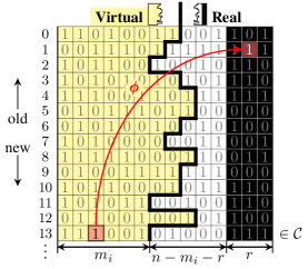
Figure 1: Example of a zipper code with a systematically encoded $\mathcal{C}_{i}=\mathcal{C}$ constituent code with $n=n_{i}=14$ and $r=r_{i}=3$. Tiles in the shaded region represent virtual symbols, while tiles in the unshaded and filled regions represent real symbols. The filled regions show the location of parity symbols. The two tiles connected by arrows represent the two coordinates prescribed by the interleaver map. In this example, we have $\phi(13,2)=(1,12)$ and $c_{13,2}=c_{1,12}=1$. Each row is a codeword of $\mathcal{C}$. Rows with lower row indices correspond to “older” rows while those with higher indices are regarded as “newer.” The icons next to “Virtual” and “Real” at the top of the figure correspond to the shape of the virtual and real buffers in the first 14 rows. The virtual and real buffers are demarcated by a bold line.

As illustrated in Fig. 1, we will partition each row of a buffer $\boldsymbol{c}$ as follows. For each $i\in\mathbb{N}$, let $A_{i}\subseteq I_{i}$ be any (fixed) subset of the information positions of $\mathcal{C}_{i}$, and let $B_{i}=[n_{i}]\setminus A_{i}$ be the complementary set of positions. The buffer positions indexed by $A_{i}$ form the virtual positions of the $i$th row (the corresponding symbols are called virtual symbols), while those indexed by $B_{i}$ form the real positions (and the corresponding symbols are called real symbols). As we will soon see, only real symbols are transmitted over the channel; each virtual symbol of a constituent codeword is a copy of a real symbol from some other constituent codeword. When $\mathcal{C}_{i}$ admits a systematic encoder, we will usually take $A_{i}=[m_{i}]$ for some $m_{i}\leq k_{i}$, thus designating the first $m_{i}$ positions as virtual positions. Let

$$A=\bigcup_{i\in\mathbb{N}}\{(i,j):j\in A_{i}\}\text{ and }B=\bigcup_{i\in\mathbb{N}}\{(i,j):j\in B_{i}\}$$

denote the positions of the virtual symbols and the real symbols, respectively. We refer to $(A,B)$ as a zipping pair. The set $\{c_{i,j}:(i,j)\in A\}$ is called the virtual buffer, and the set $\{c_{i,j}:(i,j)\in B\}$ is called the real buffer. The set $B^{*}=B\cup\{(i,j):i\in\{-1,-2,\ldots\},j\in\mathbb{N}\}$ is an index set for an extended real buffer where negative row indices are permitted. As already noted, symbols located in rows with a negative row index have value zero.

II-B Interleaver Map

An interleaver map associated with a zipping pair $(A,B)$ is any function $\phi:A\rightarrow B^{*}$. For each virtual position $(i,j)\in A$, the interleaver map gives a real position $\phi(i,j)\in B^{*}$ from which to copy a symbol.

We will often be interested in the row index from which a real symbol is copied. To this end, we define coordinate functions $\phi_{1}$ and $\phi_{2}$ such that $\phi(i,j)=(\phi_{1}(i,j),\phi_{2}(i,j))$. Thus $\phi_{1}(i,j)$ returns the row index from which the virtual symbol at position $(i,j)$ is copied. If $\phi_{1}(i,j)<0$, then the copied symbol is necessarily zero.

For each real position $(i,j)\in B^{*}$, let $\phi^{-1}(i,j)=\{(i^{\prime},j^{\prime})\in A\colon\phi(i^{\prime},j^{\prime})=(i,j)\}$ denote the inverse image of $(i,j)$ under mapping by $\phi$. Then $|\phi^{-1}(i,j)|$ gives the number of virtual copies of the real symbol in position $(i,j)$.

Equipped with a sequence $\mathcal{C}_{0},\mathcal{C}_{1},\ldots$ of constituent codes, a zipping pair $(A,B)$, and an interleaver map $\phi$, we say that a buffer $\boldsymbol{c}=\boldsymbol{c}_{0},\boldsymbol{c}_{1},\ldots$ forms a valid zipper codeword if

1. $c_{i,j}=c_{\phi(i,j)}$ for all $(i,j)\in A$, and

2. $\boldsymbol{c}_{i}\in\mathcal{C}_{i}$ for all $i\in\mathbb{N}$.

In other words, each virtual symbol of a valid zipper codeword must be a copy of a real symbol as prescribed by the interleaver map $\phi$, and each row of a valid zipper codeword must be a codeword of the corresponding constituent code.

Fig. 1 illustrates a zipper codeword in a zipper code specified in terms of a sequence of constituent codes having fixed length $n=n_{i}=14$ and fixed dimension $k=k_{i}=11$. The constituent codes are assumed to admit systematic encoders, so that parity symbols fall into the last $r=n-k=3$ positions in each row. The first $m_{i}$ positions in each row are the virtual positions, while the last $n-m_{i}$ positions are the real positions. Note that $m_{i}$ is permitted to vary from row to row. As illustrated, the interleaver map $\phi$ determines the position at which to look up the value of a virtual symbol.

It is clear that the interleaver map determines the degree of coupling among the various constituent codes. We will usually focus on interleaver maps that are periodic and causal.

Definition 1.

An interleaver map $\phi$ is said to be periodic with period $\nu>0$, or simply $\nu$-periodic, if $\phi(\nu+i,j)=(\nu,0)+\phi(i,j)$ for all $(i,j)\in A$.

To support a $\nu$-periodic interleaver map, we will require that the zipping pair $(A,B)$ is also $\nu$-periodic in the sense that $n_{\nu+i}=n_{i}$, and $A_{\nu+i}=A_{i}$ for all $i\in\mathbb{N}$. Most often we will then also have $\mathcal{C}_{\nu+i}=\mathcal{C}_{i}$ for all $i\in\mathbb{N}$.

Definition 2.

An interleaver map $\phi$ is said to be causal if $\phi_{1}(i,j)\leq i$ for all $(i,j)\in A$ and strictly causal if the inequality is strict.

In other words, under a causal interleaver map, virtual symbols are never copied from later rows.

Some important classes of zipper codes (such as staircase codes) have the property that each real symbol is copied exactly once into some virtual position, i.e., the inverse image $\phi^{-1}(i,j)$ of every real position $(i,j)\in B$ under mapping by $\phi$ is a singleton set $\{(i^{\prime},j^{\prime})\}$ for some $(i^{\prime},j^{\prime})\in A$. In this situation we refer to the interleaver map as being bijective.

II-C Encoding Zipper Codes

Recall that $I_{i}\subseteq[n_{i}]$ denotes an information set with $|I_{i}|=k_{i}$ for the constituent code $\mathcal{C}_{i}$ of length $n_{i}$ and dimension $k_{i}$, and that $A_{i}\subseteq I_{i}$ is an index set for the virtual positions of the $i$th buffer row $\boldsymbol{c}_{i}$. To encode $\boldsymbol{c}_{i}$, we assume that all rows $\boldsymbol{c}_{j}$ with $j<i$ have already been encoded. This will be true even for $c_{0}$, since previous rows are then all-zero by assumption. Under the assumption of a causal interleaver map, the encoding of zipper codes is easily accomplished by the following procedure:

1. Fill in the positions indexed by $B_{i}\cap I_{i}$ with message symbols.

2. Fill in the virtual symbols by duplicating symbols from the positions prescribed by the interleaver map, i.e., for each $j\in A_{i}$, let $c_{i,j}=c_{\phi(i,j)}$. (Since $\phi$ is causal by assumption, $c_{\phi(i,j)}$ is a symbol from a row already encoded, or a symbol from the current row which was input in the first step.)

3. Complete the row by filling in the parity symbols in positions indexed by $[n_{i}]\setminus I_{i}$ using an appropriate encoder for $\mathcal{C}_{i}$, thereby fulfilling the condition that $\boldsymbol{c}_{i}\in\mathcal{C}_{i}$.

In the zipper code of Fig. 1, for example, the shaded tiles in row $i$ are filled with symbols drawn from previous rows, the unshaded tiles correspond to message symbols, and the filled tiles correspond to parity symbols computed using the encoder for $\mathcal{C}_{i}$.

II-D Code Rate

We will always assume that only the symbols in the real buffer, i.e., in positions indexed by $B$, are transmitted over the channel, in some well-defined order from oldest to newest. The symbols in the virtual buffer, which are needed for purposes of encoding and decoding, are not transmitted. As usual, let $m_{i}=|A_{i}|$ denote the number of virtual symbols in row $i$. Under the assumption of that only the real buffer is sent, the rate of a zipper code is given as

$$R=\lim_{L\to\infty}\frac{\sum_{i=0}^{L-1}(k_{i}-m_{i})}{\sum_{i=0}^{L-1}(n_{i}-m_{i})}=\frac{\overline{k}-\overline{m}}{\overline{n}-\overline{m}},$$ (1)

where, assuming the limits exist,

$$\overline{k}=\lim_{L\to\infty}\sum_{i=0}^{L-1}\frac{k_{i}}{L},~{}\overline{n}=\lim_{L\to\infty}\sum_{i=0}^{L-1}\frac{n_{i}}{L},~{}\overline{m}=\lim_{L\to\infty}\sum_{i=0}^{L-1}\frac{m_{i}}{L}.$$

For example, staircase codes with staircase block size $m\times m$ uses a fixed constituent code of length $2m$ and dimension $k$. Thus, $\overline{n}=2m$, $\overline{k}=k$, and $\overline{m}=m$, thereby achieving a rate $R=\frac{k}{m}-1$ (assuming $\frac{k}{m}>1$).

II-E Decoding

Suppose that we transmit real symbols in positions indexed by $B$. At the receiver we can form a buffer $\boldsymbol{c}^{\prime}$ by filling in the real positions from symbols received at the output of the channel, and filling in virtual positions by copying real received symbols as prescribed by the interleaver map $\phi$. We generally assume a hard-decision channel, i.e., we assume that the channel outputs are elements of $\mathbb{F}_{2}$, though it is possible to consider more general situations with various amounts of reliability information in the form of erasures or log-likelihood ratios. The received buffer $\boldsymbol{c}^{\prime}$ is not necessarily a zipper codeword, since, due to channel noise or other impairments causing detection errors, the rows aren’t necessarily codewords of the corresponding constituent codes. Ideally, the aim of the decoder would be to recover a valid zipper codeword while making as few changes to $\boldsymbol{c}^{\prime}$ as possible. However, such optimal minimum Hamming distance decoding is often too complicated to implement, so in practice some form of iterative decoding is used, making changes to the rows one at a time using the constraints imposed only by the constituent code that constrains that row, and usually revisiting each row a number of times.

Decoding is typically performed within a sliding window of $M$ consecutive rows $\boldsymbol{c}^{\prime}_{i-M+1},\boldsymbol{c}^{\prime}_{i-M+2},\ldots,\boldsymbol{c}^{\prime}_{i}$ from the received buffer. Many of the virtual symbols in these rows will, however, be copies of symbols from outside the sliding window (which, ideally, will have been corrected by previous decoding iterations). The decoder operates by decoding the rows within the decoding window. When the decoder performs correction operations (flipping the value of one or more bits in a row), all copies of the affected bits within the decoding window (as determined by the interleaver map) will also need to be flipped. After a number of iterations have been performed, the sliding window can be advanced (by one or, more usually, several rows), and the corrected information symbols leaving the window can be delivered as the decoder output. Numerous variations of this basic scheme are possible.

In one round of so-called exhaustive decoding, every row in the decoding window is visited (exactly once) by the corresponding constituent decoder. Each bit is decoded (in a round) as many times as it appears in the window. Exhaustive decoding can be performed in serial fashion (one row at a time), or in parallel (usually under the constraint that decoders operating in parallel don’t operate on the same bits).

In one round of so-called pipelined decoding, only a subset of the rows in the decoding window (every $L$th row, say, for some parameter $L$) are visited by constituent decoders. This method may be faster than exhaustive decoding, but, depending on the interleaver map, some bits may not be visited by a decoder at all. Thus, pipelined decoding is suitable only for certain types of interleaver maps that ensure that as many bits as possible are visited by the constituent decoders. Similar to exhaustive decoding, pipelined decoding can be done in series or parallel.

Under both of these decoding methodologies, decoding can be performed in multiple rounds, until no more errors can be corrected or until some maximum number of allowed decoding rounds is reached.

Additional strategies can also be applied to these decoding procedures. In chunk decoding, rather than advancing the sliding window one row at a time, the window is advanced only after a specified number of new rows, called a chunk, is received.

In decoding with fresh/stale flags, a “fresh/stale” status indicator is maintained for each buffer row. The indicator is set to “fresh” whenever a change is made to the row (for example, if the row is newly arrived, or a bit has been flipped in that row due to a correction elsewhere); otherwise, after a decoding it is set to “stale”. In each iteration, decoders can skip over stale rows (since nothing has changed in that row since the previous iteration, and therefore the row has either been corrected or has been determined to be uncorrectable).

In decoding with periodic truncation, a fraction of the message positions are reserved to be set to known values (for example, zero). The known symbols do not need to be transmitted, as they can be filled in perfectly at the receiver. One approach would be to alternate between sending data in, say, $J$ consecutive rows, and not sending data (or, more precisely, sending only parity symbols) in $\tau$ consecutive rows. We call $J$ and $\tau$ the transmission length and truncation length, respectively. This method is a generalization of staircase code “termination” discussed in [27], and is a form of code “shortening” as defined in coding theory. The shortened code will have a lower code rate than the zipper code from which it is derived.

In dynamic decoding, the decoder is implemented with a number of constituent decoders that can operate in parallel and that can be assigned dynamically (according to a scheduling module) to the rows to be decoded. Equipping a decoding engine with the flexibility to assign decoders to the rows where work needs to be done results in increased hardware utilization (reduced computational idling). Dynamic decoding can achieve similar decoding performance with fewer computational resources than without dynamic decoding [28].

Although they fall outside the scope of this paper, a variety of soft-decision or soft-aided decoder architectures are also possible. Among these, we mention anchor decoding [29], “trusted symbol” decoding [30], soft-aided decoding [31, 32, 33, 34], and error-and-erasure decoding [2, 35].

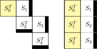
Figure 2: Staircase code (left); corresponding zipper code (right).

III Examples

This section gives some examples of related spatially-coupled codes that can be described as zipper codes. Due to space constraints, only a few codes will be described in detail, but other codes that can be described as zipper codes include those in [5, 6, 7, 8, 9, 10].

III-A Staircase Codes

Staircase codes [3] are characterized by having an infinite sequence of matrices of size $m\times m$: $S_{0},S_{1},\ldots$ such that, for each $i\in\mathbb{N}$, every row of $\begin{bmatrix}S_{i}^{T}&S_{i+1}\end{bmatrix}$ is a codeword of a constituent code $\mathcal{C}$ of length $2m$ admitting a systematic encoder, where $S_{i}^{T}$ is the transpose of $S_{i}$. The initial block $S_{0}$ is all zero (and not transmitted). The codes are so named because the sequence of matrices form a staircase-like pattern when arranged as shown in Fig. 2 (left), in which each row and each column must be a codeword of $\mathcal{C}$, and where the dark-filled regions hold parity symbols.

Staircase codes correspond to zipper codes with a fixed constituent code $\mathcal{C}$ of length $2m$ admitting a systematic encoder, and a zipping pair with $A_{i}=[m]$ for all $i\in\mathbb{N}$, i.e., the virtual positions comprise the first $m$ positions in each row. The interleaver map $\phi$ is $m$-periodic and defined to perform a transposition operation, i.e.,

$$\phi(mi+r,j)=\left(m(i-1)+j,m+r\right),\text{ for }r\in[m].$$

The resulting buffer then forms the pattern shown in Fig. 2 (right).

III-B Braided Block Codes

Braided block codes [4] are a type of convolutional code whose codewords can be represented as a subarray of an infinite two dimensional array constrained by two interacting constituent codes, one providing constraints on rows and the other providing constraints on columns. An example of a codeword from a rate $1/7$ tightly braided block code from [4] is shown in Fig. 3 (left). In this example, each row and each column in the diagram must form a codeword of the binary $(7,4)$ Hamming code. The information positions are labelled $a,b,c,\ldots$ and the positions of parity symbols are shown with dark-filled tiles.

This tightly braided block code corresponds to a zipper code with fixed $(7,4)$ Hamming constituent code. The zipping pair is defined so that $A_{i}=[3]$ when $i$ is even, and $A_{i}=[4]$ when $i$ is odd. The interleaver map is given as

$$\phi(i,j)=\begin{cases}(i+2j-5,6-j)&\text{for }i\text{ even},\\ (i-2j-3,4+j)&\text{for }i\text{ odd, }j\neq 3,\\ (i-1,3)&\text{for }i\text{ odd, }j=3,\end{cases}$$

where the last case corresponds to copying an information symbol from the row above. In this example, only even-numbered rows contain an information symbol. The name “zipper code” derives from the buffer pattern formed in this example.

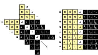
Figure 3: Tightly braided code with $(7,4)$ Hamming constituent code (left); corresponding zipper code (right), with numbers indexing constituent codewords.

III-C Diagonal Zipper Codes

In this subsection, we introduce two interleaver maps that couple the bits of a zipper code in a regular (“hardware-friendly”) fashion. These interleaver maps generalize those of staircase codes.

III-C1 Tiled Diagonal Zipper Codes

Tiled diagonal zipper codes are a generalization of staircase codes that are defined defined in terms of $w\times w$ “tiles” of symbols, a fixed constituent code $\mathcal{C}$ with length $2Lw$ admitting a systematic encoder, and a zipping pair with $A_{i}=[Lw]$ (so that virtual positions comprise the first $Lw$ positions in each buffer row), where the parameter $L$ is a positive integer. The interleaver map is defined so that each $w\times w$ tile within the virtual buffer is the transpose of some $w\times w$ tile within the real buffer, as illustrated in Fig. 4.

To specify the interleaver map precisely, we must introduce a coordinate system for tiles. For a buffer $\boldsymbol{c}$, for any $s\in[2L]$ and for any $q\in\mathbb{N}$, let

$$T_{q,s}=\left[\begin{array}[]{ccc}c_{wq,ws}&\cdots&c_{wq,ws+w-1}\\ \vdots&\ddots&\vdots\\ c_{wq+w-1,ws}&\cdots&c_{wq+w-1,ws+w-1}\end{array}\right].$$

The $w\times w$ matrix $T_{q,s}$ is a tile located within the buffer whose top left entry has position $(wq,ws)$. When $s<L$, such a tile comprises only virtual symbols, and therefore it is called a virtual tile; otherwise it is a real tile. For fixed $q$, the set of tiles $\{T_{q,s}\colon s\in[2L]\}$ are said to form the $q$th tile row.

For any $s\in[L]$ (indexing a virtual tile), we would like to have $T_{q,s}=T_{q-s-1,L+s}^{T}$. Thus the first virtual tile in tile row $q$ is the transpose of the first real tile located one tile row earlier, the second virtual tile in tile row $q$ is the transpose of the second real tile located two tile rows earlier, and so on. The interleaver map that accomplishes this task is given as

$$\phi(wq+i,ws+j)=(w(q-s-1)+j,w(L+s)+i).$$ (2)

Fig. 4 shows an example of a tiled diagonal zipper code with $L=3$.

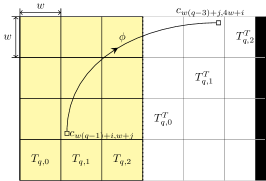
Figure 4: Tiled diagonal zipper code with $L=3$, tile size $w\times w$, and interleaver map as described in (2).

When $w=1$ (the case of $1\times 1$ tiles) tiled diagonal zipper codes recover the interleaving pattern of the continuously interleaved BCH (CI-BCH) codes described in [6]. When $L=1$, tiled diagonal zipper codes are staircase codes.

III-C2 Delayed Diagonal Zipper Codes

Delayed diagonal zipper codes are variants of tiled diagonal zipper codes with $w=1$ and an added “delay” in the interleaver map. Specifically, the interleaver map is given by

$$\phi(i,j)=(i-j-\delta,j+m),$$

where the positive integer $\delta$ is the delay parameter. When $\delta=1$, the interleaver map is identical to the interleaver map (2) with $w=1$. Fig. 5 illustrates the buffer of a delayed diagonal zipper code with $m=8$. As will show in Section V, the introduction of delay in the interleaver map reduces the multiplicity of minimal stall patterns. Delayed diagonal zipper codes can be generalized to the case of $w\times w$ tiles, with $w>1$, in the obvious way.

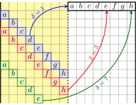
Figure 5: Delayed diagonal zipper code with $m=8$ and various delay values $\delta$.

IV Design Examples

In this section, we present software simulation results for several tiled diagonal and delayed diagonal zipper code design examples.

IV-A Simulation Setup

We simulate transmission of zipper codewords over a binary symmetric channel with crossover probability $p$. This corresponds to binary antipodal signalling over an additive white Gaussian noise channel (Bi-AWGN) with hard-decision detection, but it may also model other communications scenarios that give rise to independent and symmetrically distributed bit errors. The Shannon limit at rate $R$ for such a channel is the largest crossover probability $p$ for which it is theoretically possible to communicate at rate $R$ (bit/channel use) with arbitrarily small probability of error. For the Bi-AWGN, this value of $p$ is achieved at some particular signal-to-noise ratio (SNR). A code of finite length will achieve sufficiently small error probability only at some crossover probability smaller than the Shannon limit, corresponding to a larger Bi-AWGN SNR. The “gap to the Shannon limit” is then defined as the difference (in decibels) between the Bi-AWGN SNR corresponding to the Shannon limit and the Bi-AWGN SNR at which the code achieves sufficiently small error probability.

By “sufficiently small error probability” we mean a post-correction (post-FEC) bit error rate (BER) of $10^{-15}$ or smaller. As we cannot reliably measure such low error rates in any reasonable amount of time using software simulations, we use a least-squares fit linear extrapolation (on the log-log scale) of our measured error rates, in order to estimate the BSC crossover probability $p^{*}$ at which the post-FEC BER achieves $10^{-15}$.

In all of our design examples, we use shortened $t$-error-correcting $(n,k)$ BCH constituent codes, where $n=2m$. We made no attempt to optimize the positions at which the code is shortened. The virtual buffer and the real buffer both have width $m$. We use a causal, periodic, bijective interleaver map that implements a diagonal or delayed diagonal zipper code.

Decoding is performed using exhaustive decoding, with at most five rounds per window of size $M$ rows (thus containing $Mm$ real symbols). We use chunk decoding with chunk size $m$, fresh/stale flags, and periodic truncation with transmission length $J=995m$ and $\tau=5m$.

IV-B Varying Decoding Window Sizes

We simulated a rate $0.97$ tiled diagonal zipper code with $w=1$ and $m=1200$, (corresponding to a CI-BCH code [6]) having a $(2400,2364,t=3)$ shortened BCH constituent code, over varying decoding window sizes. As shown in Fig. 6, we observe an improvement in the decoding performance as well as disappearing error flare as we increase the decoding window sizes. This is due to the fact that larger decoding windows provide each symbol with a larger number of decoding rounds. However, as expected, we see a diminishing return as the window size increases, with only slight improvement when increasing the decoding window size from $4m^{2}=5.76$ Mb to $5m^{2}=7.20$ Mb. Simulation results for a variety of different tiled diagonal zipper codes indicate that choosing the window size near $5m^{2}$ gives nearly best possible decoding performance. This choice of window size is a convenient heuristic, akin to the well-known rule-of-thumb in convolutional decoding that suggests that a truncation depth of about five times the code’s constraint length suffices to provide nearly optimal decoding performance under Viterbi decoding (see, e.g., [36]). In a tiled diagonal zipper code with $w=1$, the parameter $m^{2}$ plays the role of constraint length, since output symbols depend on input symbols located as far as $m$ rows earlier (and each row contains $m$ real symbols).

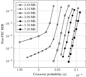
Figure 6: Simulation results of rate $0.97$ tiled diagonal zipper codes ($w=1$, $t=3$ constituent code) with different decoding window size.

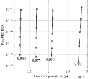
Figure 7: Simulation results of tiled diagonal zipper codes ($w=1$, $t=3$ constituent code) over different code rates. Error bars are located one standard deviation from the mean.

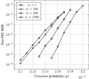
Figure 8: Simulation results of rate $0.967$ tiled diagonal zipper codes ($t=3$ constituent code) with different tile sizes.

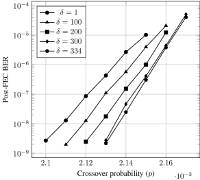
Figure 9: Simulation results of rate $0.967$ delayed diagonal zipper codes ($t=3$ constituent code) with different delay parameters.

IV-C Different Code Rates

As shown in Fig. 7, we simulated the decoding of tiled diagonal zipper codes with tile size $w=1$ having different code rates, as summarized in Table I. The decoding window (DW) size was set to $5m^{2}$ in all cases. We see that the gap to the Shannon limit decreases as the rate increases, which is consistent with the theoretical analysis of [22].

TABLE I: Simulation parameters, thresholds, and gaps to the Shannon limit.

Rate	$m$	$(n,\,k,\,t)$	DW Size	$p^{*}$	Gap (dB)
$0.960$	$825$	$(1650,1617,3)$	$3.4$ Mb	$2.68\cdot 10^{-3}$	$0.503$
$0.970$	$1200$	$(2400,2364,3)$	$7.2$ Mb	$2.03\cdot 10^{-3}$	$0.412$
$0.975$	$1440$	$(2880,2844,3)$	$10.4$ Mb	$1.63\cdot 10^{-3}$	$0.398$
$0.980$	$1800$	$(3600,3564,3)$	$16.2$ Mb	$1.24\cdot 10^{-3}$	$0.393$

IV-D Tiled Diagonal and Delayed Diagonal Zipper Codes

We simulated rate $0.967$ codes with $m=1000$, based on a $(2000,1967,t=3)$ shortened BCH constituent code, with $5$ Mb decoding window size. Various tiled and delayed diagonal zipper codes having a variety of tile sizes $w$ and delay parameter $\delta$, as summarized in Table II, were simulated. Performance curves for the tiled diagonal codes are shown in Fig. 8 and those for the delayed diagonal codes are shown in Fig. 9.

In both cases, increasing $w$ or $\delta$ helps improve the decoding with an improvement to the gap to the Shannon limit of $0.028\sim 0.039$ dB when compared to the $\delta=w=1$ case. A stall pattern analysis for tiled diagonal and delayed diagonal zipper codes, which may provide theoretical justification for these performance improvements, is given in Sec. V.

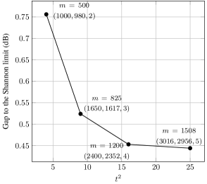
Figure 10: Gap to the Shannon limit for different decoding radius of a rate $0.96$ delayed diagonal zipper code with $\delta=1$. The values of $m$ and constituent code parameters $(n,k,t)$ are shown next to each point. In all cases, we have the decoding window size to be $5m^{2}$ bits.

TABLE II: Gap to the Shannon limit at $10^{-15}$ post-FEC BER for tiled diagonal and delayed diagonal zipper codes.

Type	$w$ or $\delta$	$p^{*}$	Gap (dB)
tiled/delayed	$1$	$2.015\cdot 10^{-3}$	$0.536$
tiled	$100$	$2.036\cdot 10^{-3}$	$0.526$
tiled	$500$	$2.060\cdot 10^{-3}$	$0.514$
tiled	$1000$	$2.099\cdot 10^{-3}$	$0.497$
delayed	$100$	$2.035\cdot 10^{-3}$	$0.526$
delayed	$200$	$2.048\cdot 10^{-3}$	$0.520$
delayed	$300$	$2.071\cdot 10^{-3}$	$0.509$
delayed	$334$	$2.073\cdot 10^{-3}$	$0.508$

IV-E Performance versus Complexity

Let us define the performance of a zipper code as its gap to the Shannon limit at $10^{-15}$ output bit error rate, and its complexity as the squared decoding radius $t^{2}$ of its constituent code. This complexity measure is chosen in view of the well-known fact that the power consumption of a Berlekamp-Massey-based BCH decoder circuits grows as $\mathcal{O}(t^{2})$ [37]. Fig. 10 plots performance versus complexity for various rate $0.96$ diagonal zipper codes. As expected, the gap to the Shannon limit is reduced by increasing the complexity of the constituent code, but with diminishing returns.

V Stall Pattern Analysis

This section will characterize stall patterns of zipper codes. For simplicity, throughout this section we will be focusing on zipper codes whose interleaver maps are bijective.

V-A Graph Representation of Zipper Codes

Due to the spatially-coupled structure of zipper codes, it can be helpful to describe them as codes defined on graphs. Following the notation of Sec. II, we consider a zipper code corresponding to constituent code sequence $\mathcal{C}_{0},\mathcal{C}_{1},\ldots$, with respective information sets $I_{0},I_{1},\ldots$. For each $i\in\mathbb{N}$, the virtual symbols in the $i$th row of a buffer are indexed by the set $A_{i}\subseteq I_{i}$. Fix a bijective interleaver map $\phi=(\phi_{1},\phi_{2})$. Let

$$\phi_{1}(A_{i})=\left\{\phi_{1}(i,j)\colon j\in A_{i}\right\}\cap\mathbb{N}$$

be the set of row indices from which the virtual symbols in row $i$ are copied (excluding any negative row indices).

Define a graph $G=(V,E)$ whose vertex set $V=\mathbb{N}$ is the set of natural numbers, and whose edge set

$$E=\{\{i,j\}:i\in\mathbb{N},j\in\phi_{1}(A_{i})\}.$$

The vertices then correspond to constituent codes, with an edge joining two vertices if the corresponding codes have a symbol in common. Parallel edges are permitted, thus we interpret the edge set as a multiset (a set in which elements may have multiplicity greater than one). The number of edges between two vertices is then equal to the number of symbols that the corresponding codes have in common. Allowing for parallel edges, the degree of vertex $i$ is equal to $n_{i}$, the block length of $\mathcal{C}_{i}$, unless some virtual symbols in row $i$ are copied from rows with negative row index, in which case the corresponding edges are missing.

Example 1.

Recall that the interleaver map of a tiled diagonal zipper code with $w=1$ is given by $\phi(i,j)=(i-j-1,m+j)$. For each $i\in\mathbb{N}$, we have $\phi_{1}(A_{i})=\{i-1,i-2,\ldots,i-m\}\cap\mathbb{N}$. Thus vertex $i$ will have neighbors

$$\mathcal{N}(i)=\{i\pm 1,i\pm 2,\ldots,i\pm m\}\cap\mathbb{N}.$$

Vertices $m,m+1,m+2,\ldots$ therefore have degree $n=2m$. The graph of a tiled diagonal zipper code with $m=4$, $w=1$ is shown in Fig. 11.

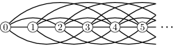
Figure 11: Graph representation of a tiled diagonal zipper code with $m=4$, $w=1$.

Graph representations for zipper codes in which symbols are copied more than once (i.e., when the interleaver map is non-bijective) can be defined by appealing to hypergraphs (in which hyperedges comprise more than two vertices), to a bipartite representation such as a factor graph, or by introducing additional constituent repetition-code constraints. We will not pursue such representations in this paper.

V-B Error and Stall Patterns

Recall that $B$ is a set containing the positions of all real symbols in a buffer. An error pattern $S\subseteq B$ is any nonempty subset of $B$ containing the positions of erroneous symbols in the real part of a received buffer. For any error pattern $S$, we define

$$S^{*}=S\cup\bigcup_{s\in S}\phi^{-1}(s)$$

to be the complete set of positions of errors and their duplicates in the virtual set, and we define $\pi(S^{*})=\{i:(i,j)\in S^{*}\}$ to be the set of affected rows.

For simplicity, throughout this section we assume that the constituent code is identical for all rows, i.e., $\mathcal{C}_{i}=\mathcal{C}$ with decoding radius $t_{i}=t$ for all $i\in\mathbb{N}$. In addition, we assume that we use a genie-aided, miscorrection-free constituent decoder. Such a decoder is able to correct up to $t$ errors in a row, but always fails to decode (never miscorrecting) when the number of errors in a row exceeds $t$. We assume that this genie-aided decoder visits rows in a decoding window as many times as is needed, reducing the error pattern size until no further correction is possible. Should some errors remain after this decoding procedure, we call the remaining errors a stall pattern. In a stall pattern, we must have at least $t+1$ errors in every remaining affected row.

We will consider only strictly causal interleaver maps that induce at most one shared symbol between any two distinct rows of a zipper code. This means that the resulting graph is simple, i.e., it contains no parallel edges or self-loops. Each edge of a such a simple graph corresponds to one codeword symbol. We refer to such an interleaver map as scattering.

V-C Decoding on a Graph

Assuming a scattering interleaver map, an error pattern $S$ can be represented as a subgraph of the graph representing the zipper code. If the zipper code has graph representation $G=(V,E)$, the graph representation of $S$ is $G_{S}=(V_{S},E_{S})$, where $V_{S}=\pi(S^{*})\subseteq V$ (i.e., the vertex set of $S$ contains vertices corresponding to the rows affected by $S$) and $E_{S}=\{\{i,j\}:(i,k)\in S,j\in\phi_{1}^{-1}(i,k)\}$ (i.e., the edges in $E_{S}$ correspond to symbols in error). From this construction, the number of edges in $G_{S}$ is exactly the cardinality of $S$. We call $|S|=|E_{S}|$ the size of the error pattern $S$.

Suppose that the constituent code $\mathcal{C}$ can correct up to $t$ errors. The action of the genie-aided decoder can then be described as an edge-peeling process in the error pattern graph $G_{S}=(V_{S},E_{S})$:

1. For each vertex $v\in V_{S}$ with $\deg(v)\leq t$, remove $v$ from $V_{S}$ as well as all edges in $E_{s}$ incident on $v$.

2. Repeat step 1 until either the graph is empty or all remaining vertices have degree $t+1$ or higher.

This procedure will terminate either in an empty graph (successful decoding), or in a $(t+1)$-core of $G_{S}$—the largest induced subgraph of $G_{S}$ with the property that all vertices have degree at least $t+1$. Sometimes, though not always, the $(t+1)$-core will form a $(t+2)$-clique, i.e., a subgraph of $G_{S}$ comprising $t+2$ vertices all of which are neighbors (a complete subgraph). Such a pattern is uncorrectable by the genie-aided decoder. More generally, we call $G_{S}$ a stall pattern if each vertex in $G_{S}$ has degree at least $t+1$, making it uncorrectable.

The following example illustrates error and stall patterns in both array and graph representations.

Example 2.

Consider a zipper code with a constituent code $\mathcal{C}$ capable of correcting $t=2$ errors. Suppose that we receive an error pattern with seven errors as shown in Figure 12. Since rows $1,3,6,$ and $8$ have at least $3$ errors each, we cannot correct them. However, we can still correct row $4$, which has only one error. Thus we will remove the error from row $4$ and its corresponding entry in row $6$, or equivalently, we remove vertex $4$ and its incident edges. However, the remaining errors cannot be corrected and so those errors form a stall pattern. The $4$-clique formed by vertices $1,3,6,$ and $8$ is a stall pattern and it is also the $3$-core of the error pattern graph from which we started.

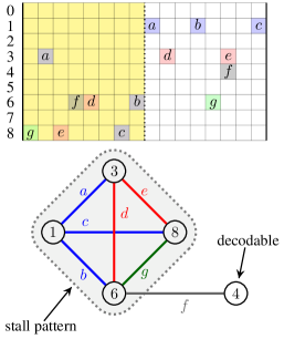
Figure 12: Example of an error pattern with underlying stall pattern in both array (top) and graph (bottom) forms. In this example, the constituent code is double-error-correcting ($t=2$).

V-D Properties of Stall Patterns of Zipper Codes

The following theorem bounds the size of a stall pattern in a zipper code with a bijective and scattering interleaver map.

Theorem 1.

A stall pattern $S$ for a zipper code with a $t$-error-correcting constituent code and having a bijective and scattering interleaver map satisfies $|S|\geq\frac{1}{2}(t+1)(t+2)$.

Proof:

Let $G_{S}=(V_{S},E_{S})$ be the graph representation of stall pattern $S$, and let $v$ be any vertex in $V_{S}$. Then, since $G_{S}$ is a stall pattern, $\deg(v)\geq t+1$. Suppose that $\mathcal{N}_{S}(v)=\{v_{1},v_{2},\ldots,v_{\deg{v}}\}$ are the neighbors of $v$ in $G_{S}$. Then, since each $v_{i}$ is a vertex in a stall pattern, $\deg(v_{i})\geq t+1$. Hence, there must be at least $\deg(v)+1\geq t+2$ vertices in $G_{S}$ with each vertex having degree $t+1$ or higher. We now apply the handshaking lemma of graph theory [38, Prop. 1.3.3.], which states that for every (finite) graph $(V,E)$ we have $\sum_{v\in V}\deg(v)=2|E|$, since each edge of the graph is counted exactly twice when summing over vertex degrees. Thus it follows that

$$|S|=|E_{S}|=\frac{1}{2}\sum_{v\in V_{S}}\deg(v)\geq\frac{1}{2}(t+1)(t+2).$$

∎

It is worth noting that $\frac{1}{2}(t+1)(t+2)$ is precisely the number of edges of a complete graph with $t+2$ vertices. In fact, we will now show that the existence of a $(t+2)$-clique in the graph representation of the zipper code is a necessary and sufficient condition for the existence of a stall pattern of size $\frac{1}{2}(t+1)(t+2)$.

Proposition 1.

Let $G=(V,E)$ be the graph representation of a zipper code with a $t$-error-correcting constituent code and a bijective and scattering interleaver map. Then the code has a stall pattern $S$ of size $\frac{1}{2}(t+1)(t+2)$ if and only if $G$ contains a $(t+2)$-clique.

Proof:

$(\Leftarrow)$ Every $(t+2)$-clique corresponds to a stall pattern of size $\frac{1}{2}(t+1)(t+2)$.
$(\Rightarrow)$ Suppose by way of contradiction that a stall pattern $S$ of size $\frac{1}{2}(t+1)(t+2)$ has a graph $G_{S}$ with more than $t+2$ vertices. The average degree of the vertices is then less than $2|S|/(t+2)=t+1$, which implies implies that $V_{S}$ contains at least one vertex of degree $t$ or lower, contradicting the fact that $S$ is a stall pattern. On the other hand, if $G_{S}$ contains fewer than $t+2$ vertices, then there exists a vertex in $V_{S}$ with degree greater than $t+1$, which is impossible in a simple graph. ∎

An example of an interleaver map that yields a stall pattern of size $\frac{1}{2}(t+1)(t+2)$ is the tiled diagonal zipper code with tile size $1$ (or delayed diagonal with delay $1$). Fig. 13 shows an example of a tiled diagonal zipper code with $w=1$, $m=3$, $t=2$.

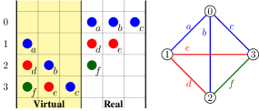
Figure 13: Graph representation of a stall pattern of size $6$ of tiled diagonal zipper code, $w=1$, $m=3$, $t=2$.

Theorem 1 can be generalized to strictly causal non-scattering interleaver maps that allow constituent codes to have up to $b$ bits in common, so that the resulting graph representation has up to $b$ parallel edges connecting any two vertices.

Theorem 2.

For a zipper code with $t$-error-correcting constituent code having a strictly causal interleaver map that allows up to $b$ parallel edges between any pair of vertices in its graph, the number of errors in a stall pattern is at least

$$\frac{1}{2}\left(1+\left\lceil\frac{t+1}{b}\right\rceil\right)(t+1).$$

Proof:

Any vertex in a stall pattern graph must have at least $\lceil(t+1)/b\rceil$ neighbors. The result then follows from the same argument as in the proof of Theorem 1. ∎

V-E Error Floor Approximation

The presence of stall patterns creates so-called “error floors” in the performance curves of zipper codes. We may approximate the location of the error floor using a union bound technique similar that used in [3]. We consider a decoding window of size $M\times m$, and denote the set of all stall patterns in the decoding window to be $\mathcal{S}$. We determine the error floor estimate by enumeration of $\mathcal{S}$, evaluating (an upper bound on) the probability that the particular error pattern arises at the output of a binary symmetric channel with crossover probability $p$. This then gives

$$\text{BER}_{\text{floor}}\leq\frac{1}{Mm}\sum_{S\in\mathcal{S}}|S|p^{|S|}.$$ (3)

Suppose that we could determine exactly the sizes of stall patterns that can occur in a decoding window. We could then rewrite (3) as

$$\text{BER}_{\text{floor}}\leq\frac{1}{Mm}\sum_{\ell\in\mathcal{L}}N_{\ell}p^{\ell},$$ (4)

where $\mathcal{L}$ denotes the set of all stall-pattern sizes that can occur in the decoding window of size $Mm$ and $N_{\ell}$ denotes the number of occurrences of stall patterns of size $\ell$. Note that since we only consider stall patterns that can fit in the decoding window, we have $\ell\leq Mm$.

The possible sizes and the number of occurrences of stall patterns of certain size depend on the interleaver map. For example, it is possible to construct stall patterns of size $\frac{1}{2}(t+1)(t+2)$ in tiled diagonal zipper codes with tile size $1$, but not in staircase codes, whose smallest stall pattern size is $(t+1)^{2}$ [3, 39].

Given a decoding window, a set $\mathcal{L}$ of possible stall pattern sizes that can fit in the window, and crossover probability $p$, we call the stall patterns of size $\ell^{*}\in\mathcal{L}$ to be dominant if $N_{\ell^{*}}p^{\ell^{*}}\geq N_{\ell}p^{\ell}$ for all $\ell\in\mathcal{L}$. In general, the minimum-sized stall patterns may not be dominant since it is possible that the multiplicity of larger stall patterns causes a dominant $N_{\ell}p^{\ell}$ term. However, for sufficiently small $p$, we can assume that stall patterns of minimum size are dominant. The error floor can be then further approximated as the contribution of just the minimum-sized stall patterns, i.e., the right hand side of (4) is approximately $N_{\ell^{*}}p^{\ell^{*}}$, where $\ell^{*}=\min\mathcal{L}$.

V-F Eliminating Small-Sized Stall Patterns of Diagonal Zipper Codes

We will now describe a few strategies to eliminate stall patterns of size $\frac{1}{2}(t+1)(t+2)$ in tiled and delayed diagonal zipper codes.

V-F1 Tiled Diagonal

Our first observation is that we can reduce the multiplicity stall patterns of size $\frac{1}{2}(t+1)(t+2)$ by increasing the tile size. To see this, we will first count the occurrences of stall patterns of size $\frac{1}{2}(t+1)(t+2)$. Denote the tile size as $w$ and assume that $m=wL$, $M=wK$ ($K>L$), and $L\geq t+1$. In order to construct a stall pattern of size $\frac{1}{2}(t+1)(t+2)$, we first pick $t+1$ tiles from the same row. We then select a row index at which to place the errors. For each of the $t+1$ tiles, pick one column index at which to place an error. Those errors will correspond to errors in $t+1$ other rows. The positions of the remaining $\frac{1}{2}t(t+1)$ errors in those rows are then forced. Thus, the number of stall patterns of size $\frac{1}{2}(t+1)(t+2)$ is given by

$$\sum_{s=t}^{L-1}\binom{s}{t}(K-s-1)w^{t+2}\approx\binom{L}{t+1}Kw^{t+2}.$$ (5)

Having larger tile size will make the values for $K$ and $L$ lower assuming that the decoding window size is fixed. This will in turn reduce the multiplicity of stall patterns of size $\frac{1}{2}(t+1)(t+2)$ given by (5). Furthermore once $L\leq t$, it is impossible to form a stall pattern of size $\frac{1}{2}(t+1)(t+2)$.

V-F2 Delayed Diagonal

In delayed diagonal zipper codes, the occurrences and size of the minimum-sized stall patterns depends on $\delta$. In particular, we will show that having larger delay reduces the multiplicity of stall patterns of size $\frac{1}{2}(t+1)(t+2)$.

Proposition 2.

For a delayed diagonal zipper code with $t$-error-correcting constituent code and delay parameter $\delta$, there exists a stall pattern of size $\frac{1}{2}(t+1)(t+2)$ if and only if $\delta\leq\frac{m-1}{t}$.

Proof:

Without loss of generality, let the first affected row index of the stall pattern be zero.
$(\Leftarrow)$ We claim that we can form a stall pattern of size $\frac{1}{2}(t+1)(t+2)$ whose set of row indices is given by $I=\{0,\delta,2\delta,\ldots,(t+1)\delta\}$. To see this, first observe that $(t+1)\delta=t\delta+\delta\leq m+\delta-1$. The neighbors of row $i$ in the full zipper code graph are then indexed by

$$\mathcal{N}(i)=\{i\pm(\delta+j):j\in[m]\}\cap\mathbb{N}.$$

Thus, $i+(t+1)\delta\leq\max(\mathcal{N}(i))$ and $\max\{0,i-(t+1)\delta\}\geq\min(\mathcal{N}(i))$, so $I\subseteq\mathcal{N}(i)$ for all $i\in I$. It follows that the rows in $I$ are connected with each other and so it is possible to form a $(t+2)$-clique from $I$.
$(\Rightarrow)$ Let $I=\{0,i_{1},\ldots,i_{t+1}\}$ with $0<i_{i}<\ldots<i_{t+1}$ be the row indices of a stall pattern of size $\frac{1}{2}(t+1)(t+2)$. Then it must be true that

$$i_{1} \geq 0+\delta=\delta,$$

$$i_{2} \geq i_{1}+\delta\geq 2\delta,$$

$$\vdots$$

$$i_{t+1} \geq i_{t}+\delta\geq(t+1)\delta.$$

However, we also require that row $i_{t+1}$ to be a neighbor of the first row, i.e., we require $i_{t+1}\leq m+\delta-1$. Hence, $(t+1)\delta\leq m+\delta-1$, and rearranging yields $\delta\leq\frac{m-1}{t}$. ∎

Suppose that $\delta\leq\frac{m-1}{t}$. In order to construct a stall pattern of size $\frac{1}{2}(t+1)(t+2)$ with the set of affected row index $I=\{i_{0}=0,i_{1},\ldots,i_{t+1}\}$, the following constraints must be satisfied:

• Errors in row $0$ must affect row $i_{t+1}$, i.e., $i_{t+1}\leq\delta+m-1$.

• For $j=1,\ldots,t+1$, $i_{j}-i_{j-1}\geq\delta$.

Thus, the indices $i_{1},\ldots,i_{t+1}$ must be taken from $\{\delta,\delta+1,\ldots,\delta+m-1\}$ and any two indices must differ by at least $\delta$. The number of possible combinations of such indices is given by

$$\binom{m-t(\delta-1)}{t+1}=\binom{m-t\delta+t}{t+1}.$$

In a decoding window with $M$ rows, the number of possible combinations is therefore at most

$$M\binom{m-t\delta+t}{t+1}.$$

Example 3.

Figure 14 shows the number of stall patterns of size $\frac{1}{2}(t+1)(t+2)$ involving the first row of the decoding window in delayed diagonal zipper codes for $m=1000$ and $t=3,4,5$. Observe that when $\delta=1$ and $t=3$, there are

$$\binom{1000}{4}\approx 4.14\times 10^{10}$$

possible configurations involving the first row. However, there is only one possible configuration for $\delta=333$ and stall patterns of size $\frac{1}{2}(t+1)(t+2)$ do not exist for $\delta\geq 334$.

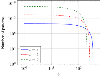
Figure 14: Number of stall patterns of size $\frac{1}{2}(t+1)(t+2)$ involving the first row of the decoding window in delayed diagonal zipper codes with $m=1000$ and varying $t,\delta$.

VI Conclusions

Zipper codes provide a convenient framework for describing a wide variety of spatially-coupled product-like codes. Such codes are of interest in high-throughput communication systems because they can be decoded iteratively using low-complexity power-efficient constituent decoders while achieving a gap to the Shannon limit on the binary symmetric channel of 0.5 dB or less at high code rates. We have introduced tiled diagonal and delayed diagonal interleaver maps that couple the constituent codes in regular (hardware-friendly) patterns. These interleaver maps provide flexibility in trading off decoding window size and code performance. A combinatorial analysis of stall patterns that arise with such interleaver maps shows that increasing tile size or delay can indeed have a beneficial effect on reducing the error floor of the code.

Further research on zipper codes is needed to address the design of interleaver maps that give rise to codes with large minimum Hamming distance or large dominant stall-pattern size. Tradeoffs between code performance and decoding latency should be better characterized. Can soft-decision (or soft-aided) decoding methods be introduced without excessive increase in decoding complexity and decoder power consumption? No doubt many further interesting questions can be formulated.

Alvin Y. Sukmadji (S’20) received the B.A.Sc. degree (with high honours) in electrical engineering with a minor in mathematics in 2017, and the M.A.Sc degree in electrical and computer engineering in 2020, both from the University of Toronto, Toronto, ON, Canada. He is currently a Ph.D. student in the Department of Electrical and Computer Engineering at the University of Toronto. His research interests include coding theory and fiber-optic communications. He received the NSERC CGS-M scholarship in 2017, the Ontario Graduate Scholarship in 2018 and 2019, and the NSERC PGS-D scholarship in 2020.

Umberto Martínez-Peñas (S’15–M’18) received the B.Sc. and M.Sc. degrees in Mathematics from the University of Valladolid, Spain, in 2013 and 2014, respectively, and the Ph.D. degree in Mathematics from Aalborg University, Denmark, in 2017. In 2018 and 2019, he was a Post-Doctoral Fellow with the Department of Electrical and Computer Engineering, University of Toronto, Canada. In 2020 and 2021, he was a Maître Assistant with the Institute of Computer Science and Mathematics, University of Neuchâtel, Switzerland. His research interests include algebra, algebraic coding, distributed storage, network coding, and information-theoretic security and privacy. He was awarded an Elite Research Travel Grant (EliteForsk Rejsestipendium) from the Danish Ministry of Education and Science in 2016, the Ph.D. Dissertation Prize by the Danish Academy of Natural Sciences (Danmarks Naturvidenskabelige Akademi, DNA) in 2018, and a Vicent Caselles Prize for Research in Mathematics by the Royal Spanish Mathematical Society (Real Sociedad Matemática Española, RSME) in 2019.

Frank R. Kschischang (S’83–M’91–SM’00–F’06) received the B.A.Sc. degree (with honours) from the University of British Columbia, Vancouver, BC, Canada, in 1985 and the M.A.Sc. and Ph.D. degrees from the University of Toronto, Toronto, ON, Canada, in 1988 and 1991, respectively, all in electrical engineering. Since 1991 he has been a faculty member in Electrical and Computer Engineering at the University of Toronto. His research interests are focused primarily on the area of channel coding techniques, applied to wireline, wireless and optical communication systems and networks. He has received several awards for teaching and research, including the 2010 Communications Society and Information Theory Society Joint Paper Award, and the 2018 IEEE Information Theory Society Paper Award. He is a Fellow of IEEE, of the Engineering Institute of Canada, of the Canadian Academy of Engineering, and of the Royal Society of Canada. During 1997–2000, he served as an Associate Editor for Coding Theory for the IEEE Transactions on Information Theory, and from 2014–16, he served as this journal’s Editor-in-Chief. He served as general co-chair for the 2008 IEEE International Symposium on Information Theory, and he served as the 2010 President of the IEEE Information Theory Society. He received the Society’s Aaron D. Wyner Distinguished Service Award in 2016.

References

- [1] A. Y. Sukmadji, U. Martínez-Peñas, and F. R. Kschischang, “Zipper codes: Spatially-coupled product-like codes with iterative algebraic decoding,” in 16th Canadian Workshop on Information Theory (CWIT), Jun. 2019.
- [2] A. Y. Sukmadji, “Zipper codes: High-rate spatially-coupled codes with algebraic component codes,” Master’s thesis, University of Toronto, Canada, 2020.
- [3] B. P. Smith, A. Farhood, A. Hunt, F. R. Kschischang, and J. Lodge, “Staircase codes: FEC for 100 Gb/s OTN,” J. Lightw. Technol., vol. 30, no. 1, pp. 110–117, Nov. 2012.
- [4] A. Jiménez Feltström, D. Truhachev, M. Lentmaier, and K. S. Zigangirov, “Braided block codes,” IEEE Trans. Inf. Theory, vol. 55, no. 6, pp. 2640–2658, Jun. 2009.
- [5] C. P. M. J. Baggen and L. M. G. M. Tolhuizen, “On diamond codes,” IEEE Trans. Inf. Theory, vol. 43, no. 5, pp. 1400–1411, Sep. 1997.
- [6] T. Coe, “Continuously interleaved error correction,” U.S. Patent 8 276 047, Sep., 2012.
- [7] P. Northcott, “Cyclically interleaved dual BCH, with simultaneous decode and per-codeword maximum likelihood reconciliation,” U.S. Patent 8 479 084, Jul., 2013.
- [8] P. Humblet, “Forward error correction systems and methods,” U.S. Patent 10 201 026 B1, Jun., 2017.
- [9] Flexible OTN Long-Reach Interfaces, ITU-T Std. G.709.3/Y.1331.3, 2020.
- [10] G. Montorsi and S. Benedetto, “Design of spatially coupled turbo product codes for optical communications,” in 2021 11th International Symposium on Topics in Coding (ISTC), Sep. 2021, pp. 1–5.
- [11] M. Barakatain, D. Lentner, G. Böecherer, and F. R. Kschischang, “Performance-complexity tradeoffs of concatenated FEC for higher-order modulation,” J. Lightw. Technol., vol. 38, no. 11, pp. 2944–2953, Mar. 2020.
- [12] S. Stern, M. Barakatain, F. Frey, J. Pfeiffer, J. K. Fischer, and R. F. Fischer, “Coded modulation for four-dimensional signal constellations with concatenated non-binary forward error correction,” in 2020 European Conference on Optical Commun, (ECOC), Dec. 2020, pp. 1–4.
- [13] M. Barakatain and F. R. Kschischang, “Low-complexity rate- and channel-configurable concatenated codes,” J. Lightw. Technol., vol. 39, no. 7, pp. 1976–1983, Dec. 2021.
- [14] T. Mehmood, M. P. Yankov, and S. Forchhammer, “Rate-adaptive concatenated multilevel coding with fixed decoding complexity,” in 2021 11th International Symposium on Topics in Coding (ISTC), Sep. 2021, pp. 1–5.
- [15] Y. Tian, Y. Lin, J. Zheng, J. Tang, Q. Huang, H. Ma, T. Rahman, M. Kuschnerov, R. Leung, and L. Zhang, “800Gb/s-FR4 specification and interoperability analysis,” in 2021 Optical Fiber Communications Conference and Exhibition (OFC), Jun. 2021, pp. 1–3.
- [16] “200G per lane for future 800G and 1.6T modules white paper,” 800G Pluggable MSA group, White Paper, 2021. [Online]. Available: https://www.800gmsa.com/documents/200g-per-lane-for-future-800g-and-16t-modules
- [17] Q. Xie, Z. Luo, S. Xiao, K. Wang, and Z. Yu, “High-throughput zipper encoder for 800G optical communication system,” in 2021 IEEE International Conference on Integrated Circuits, Technologies and Applications (ICTA), Nov. 2021, pp. 214–215.
- [18] C. Fougstedt and P. Larsson-Edefors, “Energy-efficient high-throughput VLSI architectures for product-like codes,” J. Lightw. Technol., vol. 37, no. 2, pp. 477–485, Jan. 2019.
- [19] D. Truhachev, K. El-Sankary, A. Karami, A. Zokaei, and S. Li, “Efficient implementation of 400 Gbps optical communication FEC,” IEEE Trans. Circuits Syst. I, vol. 68, no. 1, pp. 496–509, Jan. 2021.
- [20] D. J. Costello, D. G. M. Mitchell, P. M. Olmos, and M. Lentmaier, “Spatially coupled generalized LDPC codes: Introduction and overview,” in 2018 IEEE 10th International Symposium on Turbo Codes Iterative Information Processing (ISTC), Nov. 2018, pp. 1–6.
- [21] D. G. M. Mitchell, P. M. Olmos, M. Lentmaier, and D. J. Costello, “Spatially coupled generalized LDPC codes: Asymptotic analysis and finite length scaling,” IEEE Trans. Inf. Theory, vol. 67, no. 6, pp. 3708–3723, Apr. 2021.
- [22] Y. Jian, H. D. Pfister, and K. R. Narayanan, “Approaching capacity at high rates with iterative hard-decision decoding,” IEEE Trans. Inf. Theory, vol. 63, no. 9, pp. 5752–5773, Sep. 2017.
- [23] M. Lentmaier, I. Andriyanova, N. Hassan, and G. Fettweis, “Spatial coupling - a way to improve the performance and robustness of iterative decoding,” in Proc. 2015 Eur. Conf. Netw. and Comm., Jun. 2015, pp. 1–2.
- [24] M. Weiner, M. Blagojevic, S. Skotnikov, A. Burg, P. Flatresse, and B. Nikolic, “27.7 A scalable 1.5-to-6Gb/s 6.2-to-38.1mW LDPC decoder for 60GHz wireless networks in 28nm UTBB FDSOI,” in 2014 IEEE Int. Solid-State Circuits Conf., Feb. 2014, pp. 464–465.
- [25] T. Ou, Z. Zhang, and M. C. Papaefthymiou, “27.6 an 821MHz 7.9Gb/s 7.3pJ/b/iteration charge-recovery LDPC decoder,” in 2014 IEEE Int. Solid-State Circuits Conf., Feb. 2014, pp. 462–463.
- [26] Y. Lee, H. Yoo, J. Jung, J. Jo, and I. Park, “A 2.74-pJ/bit, 17.7-Gb/s iterative concatenated-BCH decoder in 65-nm CMOS for NAND flash memory,” IEEE J. Solid-State Circuits, vol. 48, no. 10, pp. 2531–2540, Oct. 2013.
- [27] M. Qiu, L. Yang, Y. Xie, and J. Yuan, “Terminated staircase codes for NAND flash memories,” IEEE Trans. Commun., vol. 66, no. 12, pp. 5861–5875, Aug. 2018.
- [28] K. Huang, S. Xiao, D. Chang, X. Yang, Q. Huang, H. Ma, and W. K. Leung, “Dynamic decoding of zipper codes,” in 2021 Optical Fiber Commun. Conf. and Exhibition (OFC), Jun. 2021, pp. 1–3.
- [29] C. Häger and H. D. Pfister, “Approaching miscorrection-free performance of product codes with anchor decoding,” IEEE Trans. Commun., vol. 66, no. 7, pp. 2797–2808, Mar. 2018.
- [30] C. Senger, “Improved iterative decoding of product codes based on trusted symbols,” in 2019 IEEE International Symposium on Information Theory (ISIT), Jul. 2019, pp. 1342–1346.
- [31] Y. Lei, B. Chen, G. Liga, X. Deng, Z. Cao, J. Li, K. Xu, and A. Alvarado, “Improved decoding of staircase codes: The soft-aided bit-marking (SABM) algorithm,” IEEE Transactions on Communications, vol. 67, no. 12, pp. 8220–8232, Oct. 2019.
- [32] Y. Lei, B. Chen, G. Liga, A. Balatsoukas-Stimming, K. Sun, and A. Alvarado, “A soft-aided staircase decoder using three-level channel reliabilities,” J. Lightw. Technol., vol. 39, no. 19, pp. 6191–6203, Jul. 2021.
- [33] A. Sheikh, A. Graell i Amat, G. Liva, and A. Alvarado, “Refined reliability combining for binary message passing decoding of product codes,” J. Lightw. Technol., vol. 39, no. 15, pp. 4958–4973, May 2021.
- [34] A. Sheikh, A. G. i. Amat, and A. Alvarado, “Novel high-throughput decoding algorithms for product and staircase codes based on error-and-erasure decoding,” J. Lightw. Technol., vol. 39, no. 15, pp. 4909–4922, May 2021.
- [35] L. Rapp and L. Schmalen, “Error-and-erasure decoding of product and staircase codes,” IEEE Trans. Commun., vol. 70, no. 1, pp. 32–44, Jan. 2022.
- [36] G. D. Forney Jr., “Convolutional codes II. Maximum-likelihood decoding,” Information and Control, vol. 25, no. 3, pp. 222–266, 1974.
- [37] W. Liu, J. Rho, and W. Sung, “Low-power high-throughput BCH error correction VLSI design for multi-level cell NAND flash memories,” in Proc. 2006 IEEE Workshop Signal Process. Syst. Design and Implementation, Oct. 2006, pp. 303–308.
- [38] D. B. West, Introduction to Graph Theory, 2nd ed. Prentice Hall, Sep. 2000.
- [39] L. Holzbaur, H. Bartz, and A. Wachter-Zeh, “Improved decoding and error floor analysis of staircase codes,” Designs, Codes and Cryptography, vol. 87, no. 2, pp. 647–664, Mar. 2019.