Explaining the hints for lepton flavour universality violation with three $S_{2}$ leptoquark generations

Abstract

Leptoquarks are prime candidates for explaining the intriguing hints for lepton flavour universality violation. In particular, the $SU(2)_{L}$ doublet of scalar leptoquarks $S_{2}$ is capable of providing an explanation for the tensions between the measurements and the Standard Model predictions in $(g-2)_{\mu}$, $b\to s\ell^{+}\ell^{-}$ and $b\to c\tau\nu$ processes, as well as in non-resonant di-electron production. However, in the minimal setup with a single leptoquark generation, a common explanation for all these issues is not possible as this would lead to unacceptably large charged lepton flavour violation. We therefore propose a model with three generations of $S_{2}$, each coupling exclusively to a single lepton flavour, i.e. a model extending the Standard Model particle content by an electroquark, a muoquark and a tauquark. We show that after taking into account other constraints, such as those originating from electroweak precision observables and $\Delta F=2$ processes, it is possible to provide a combined explanation for all these hints of lepton flavour universality violation. Moreover, we find that the presence of the tauquark can generate a dimension-six ${\cal O}_{9}^{U}$ operator via off-shell photon penguin diagrams, which, together with the muoquark contribution, further improves the global fit to $b\to s\ell^{+}\ell^{-}$ data.

1 Introduction

The Standard Model (SM) of particle physics has been tested extensively and confirmed within the last decades, culminating in the discovery of its last missing piece, the Higgs boson, in 2012 at the LHC ATLAS:2012yve ; CMS:2012qbp . Nonetheless, it is evident that the SM cannot be the ultimate theory of nature, as it cannot for example account for dark matter or non-vanishing neutrino masses. However, these phenomena can be accounted for by new physics (NP), which could a priori lie within a wide energy range (i.e. from the keV to the scale of Grand Unification), and is therefore not necessarily within the reach of current or even future colliders.

Fortunately, in recent years exciting hints for lepton flavour universality violation (LFUV) beyond the SM have been accumulated (see e.g. Refs. Fischer:2021sqw ; Crivellin:2021sff for recent reviews), and an explanation of these anomalies requires TeV-scale new physics. This makes a discovery at the LHC possible, and an observation at future colliders even guaranteed. In particular, measurements of $b\to s\ell^{+}\ell^{-}$ CMS:2014xfa ; Aaij:2015oid ; Abdesselam:2016llu ; Aaij:2017vbb ; Aaij:2019wad ; Aaij:2020nrf ; LHCb:2021trn ; BELLE:2019xld ; Belle:2019oag ; LHCb:2016ykl ; LHCb:2021zwz ; LHCb:2020zud and $b\to c\tau\nu$ Lees:2012xj ; Lees:2013uzd ; Aaij:2015yra ; Aaij:2017deq ; Aaij:2017uff ; Abdesselam:2019dgh observables deviate from their corresponding SM predictions by more than $7\,\sigma$ Altmannshofer:2021qrr ; Geng:2021nhg ; Alguero:2021anc ; Hurth:2021nsi ; Kowalska:2019ley ; Ciuchini:2021smi ; DAmico:2017mtc ; Arbey:2019duh ; Kumar:2019nfv (this tension being reduced to $4\!-\!5\sigma$ when including only LFUV observables Altmannshofer:2021qrr ; Geng:2021nhg ; Alguero:2021anc ; Hurth:2021nsi ; Isidori:2021vtc ) and by more than $3\,\sigma$ HFLAV:2019otj respectively. Moreover, measurements of the anomalous magnetic moment of the muon $(g-2)_{\mu}$ Muong-2:2006rrc ; Muong-2:2021ojo are known to deviate from the SM predictions by more than $4\,\sigma$ when following the community consensus Aoyama:2020ynm . The latter is based on the results of Refs. Aoyama:2012wk ; Aoyama:2019ryr ; Czarnecki:2002nt ; Gnendiger:2013pva ; Davier:2017zfy ; Keshavarzi:2018mgv ; Colangelo:2018mtw ; Hoferichter:2019gzf ; Davier:2019can ; Keshavarzi:2019abf ; Kurz:2014wya ; Melnikov:2003xd ; Masjuan:2017tvw ; Colangelo:2017fiz ; Hoferichter:2018kwz ; Gerardin:2019vio ; Bijnens:2019ghy ; Colangelo:2019uex ; Blum:2019ugy ; Colangelo:2014qya that do not include the recent lattice findings of the Budapest-Marseilles-Wuppertal collaboration (BMWc) for the hadronic vacuum polarisation (HVP) contributions Borsanyi:2020mff . Whereas they render the SM predictions for $a_{\mu}$ compatible with data, the BMWc results are in tension with the HVP value determined from $e^{+}e^{-}\to$ hadrons data Davier:2017zfy ; Keshavarzi:2018mgv ; Colangelo:2018mtw ; Hoferichter:2019gzf ; Davier:2019can ; Keshavarzi:2019abf . Furthermore, HVP also enters global electroweak (EW) fits Passera:2008jk , and its (indirect) determination leads to a value smaller than that obtained by the BMWc Haller:2018nnx . Therefore, making use of the BMWc predictions for the HVP contributions to $a_{\mu}$ would increase the tension originating from the EW fits Crivellin:2020zul ; Keshavarzi:2020bfy , and we opted for omitting it until the situation gets clarified.

Prime examples that can address most, if not even all, LFUV anomalies are models featuring leptoquarks (LQs), hypothetical new particles with common couplings to quarks and leptons. LQs were originally proposed in the Pati-Salam model Pati:1974yy and in Grand Unified Theories (GUTs) Georgi:1974sy ; Dimopoulos:1980hn ; Senjanovic:1982ex ; Frampton:1989fu ; Witten:1985xc , and it has been shown that the anomalies in $b\to s\ell^{+}\ell^{-}$ Alonso:2015sja ; Calibbi:2015kma ; Hiller:2016kry ; Bhattacharya:2016mcc ; Buttazzo:2017ixm ; Barbieri:2015yvd ; Barbieri:2016las ; Calibbi:2017qbu ; Crivellin:2017dsk ; Bordone:2018nbg ; Kumar:2018kmr ; Crivellin:2018yvo ; Crivellin:2019szf ; Cornella:2019hct ; Bordone:2019uzc ; Bernigaud:2019bfy ; Aebischer:2018acj ; Fuentes-Martin:2019ign ; Popov:2019tyc ; Fajfer:2015ycq ; Blanke:2018sro ; deMedeirosVarzielas:2019lgb ; deMedeirosVarzielas:2015yxm ; Crivellin:2019dwb ; Saad:2020ihm ; Saad:2020ucl ; Gherardi:2020qhc ; DaRold:2020bib ; Greljo:2021xmg , $R(D^{(*)})$ Alonso:2015sja ; Calibbi:2015kma ; Fajfer:2015ycq ; Bhattacharya:2016mcc ; Buttazzo:2017ixm ; Barbieri:2015yvd ; Barbieri:2016las ; Calibbi:2017qbu ; Bordone:2017bld ; Bordone:2018nbg ; Kumar:2018kmr ; Biswas:2018snp ; Crivellin:2018yvo ; Blanke:2018sro ; Heeck:2018ntp ; deMedeirosVarzielas:2019lgb ; Cornella:2019hct ; Bordone:2019uzc ; Sahoo:2015wya ; Chen:2016dip ; Dey:2017ede ; Becirevic:2017jtw ; Chauhan:2017ndd ; Becirevic:2018afm ; Popov:2019tyc ; Fajfer:2012jt ; Deshpande:2012rr ; Freytsis:2015qca ; Bauer:2015knc ; Li:2016vvp ; Zhu:2016xdg ; Popov:2016fzr ; Deshpand:2016cpw ; Becirevic:2016oho ; Cai:2017wry ; Altmannshofer:2017poe ; Kamali:2018fhr ; Mandal:2018kau ; Azatov:2018knx ; Wei:2018vmk ; Angelescu:2018tyl ; Kim:2018oih ; Aydemir:2019ynb ; Crivellin:2019qnh ; Yan:2019hpm ; Crivellin:2017zlb ; Marzocca:2018wcf ; Fuentes-Martin:2020pww ; Bigaran:2019bqv ; Crivellin:2019dwb ; Saad:2020ihm ; Dev:2020qet ; Saad:2020ucl ; Altmannshofer:2020axr ; Fuentes-Martin:2020bnh ; Gherardi:2020qhc ; DaRold:2020bib , $b\to c\tau\nu$ Alonso:2015sja ; Calibbi:2015kma ; Fajfer:2015ycq ; Bhattacharya:2016mcc ; Buttazzo:2017ixm ; Barbieri:2015yvd ; Barbieri:2016las ; Calibbi:2017qbu ; Bordone:2017bld ; Bordone:2018nbg ; Kumar:2018kmr ; Biswas:2018snp ; Crivellin:2018yvo ; Blanke:2018sro ; Heeck:2018ntp ; deMedeirosVarzielas:2019lgb ; Cornella:2019hct ; Bordone:2019uzc ; Sahoo:2015wya ; Chen:2016dip ; Dey:2017ede ; Becirevic:2017jtw ; Chauhan:2017ndd ; Becirevic:2018afm ; Popov:2019tyc ; Fajfer:2012jt ; Deshpande:2012rr ; Freytsis:2015qca ; Bauer:2015knc ; Li:2016vvp ; Zhu:2016xdg ; Popov:2016fzr ; Deshpand:2016cpw ; Becirevic:2016oho ; Cai:2017wry ; Altmannshofer:2017poe ; Kamali:2018fhr ; Mandal:2018kau ; Azatov:2018knx ; Wei:2018vmk ; Angelescu:2018tyl ; Kim:2018oih ; Aydemir:2019ynb ; Crivellin:2019qnh ; Yan:2019hpm ; Crivellin:2017zlb ; Marzocca:2018wcf ; Bigaran:2019bqv ; Crivellin:2019dwb ; Saad:2020ihm ; Dev:2020qet ; Saad:2020ucl ; Altmannshofer:2020axr ; Fuentes-Martin:2020bnh ; Gherardi:2020qhc ; DaRold:2020bib ; Endo:2021lhi ; Belanger:2021smw ; Lee:2021jdr , and $(g-2)_{\mu}$ Bauer:2015knc ; Djouadi:1989md ; Chakraverty:2001yg ; Cheung:2001ip ; Popov:2016fzr ; Chen:2016dip ; Biggio:2016wyy ; Davidson:1993qk ; Couture:1995he ; Mahanta:2001yc ; Queiroz:2014pra ; ColuccioLeskow:2016dox ; Chen:2017hir ; Das:2016vkr ; Crivellin:2017zlb ; Cai:2017wry ; Crivellin:2018qmi ; Kowalska:2018ulj ; Dorsner:2019itg ; Crivellin:2019dwb ; DelleRose:2020qak ; Saad:2020ihm ; Bigaran:2020jil ; Dorsner:2020aaz ; Fuentes-Martin:2020bnh ; Gherardi:2020qhc ; Babu:2020hun ; Crivellin:2020tsz ; Marzocca:2021azj ; Wang:2021uqz ; Perez:2021ddi can all be explained by them. Moreover, LQs can provide an explanation for the CMS excess in non-resonant di-electron production Crivellin:2021egp ; Crivellin:2021bkd .

In this context, models including a $SU(2)_{L}$ leptoquark doublet $S_{2}$ that transforms under the SM gauge group $SU(3)_{c}\times SU(2)_{L}\times U(1)_{Y}$ as $\left(\mathbf{3},\mathbf{2},\frac{7}{6}\right)$, from now on called $\Phi_{2}$ (in the literature also called $R_{2}$), are particularly interesting. This LQ can restore the agreement between theory and data for $b\to s\ell^{+}\ell^{-}$ observables via a $W$-box contribution Becirevic:2017jtw , for $b\to c\tau\nu$ observables and the excess Crivellin:2021rbf in CMS di-lepton data CMS:2021ctt via tree-level contributions Crivellin:2021egp ; Crivellin:2021bkd , and for $(g-2)_{\mu}$ via an $m_{t}/m_{\mu}$ chirally enhanced effect. Furthermore, the tension in the difference of the $B\to D^{*}\ell\nu$ forward-backward asymmetries ($\Delta A_{\rm FB}$) Belle:2018ezy ; Bobeth:2021lya can be softened Crivellin:2020mjs , and the global EW fit can be improved through the generation of a shift in the $W$-boson mass predictions Crivellin:2020ukd , where a constructive effect is currently preferred deBlas:2021wap , via LQ interactions with the Higgs field Crivellin:2021ejk .

However, a combined explanation of the flavour anomalies in the minimal setup with a single leptoquark $S_{2}$ is not possible as this would lead to unacceptably large charged lepton flavour violation (LFV). In order to avoid this, we propose to extend the SM by three generations of leptoquarks, like the three generations of squarks in minimal $R$-parity violating supersymmetry Barger:1989rk ; Barbier:2004ez . In this setup each LQ flavour couples to the corresponding lepton flavour, i.e. the electroquark $\Phi_{2,e}$ coupling to electrons, the muoquark $\Phi_{2,\mu}$ to muons and the tauquark $\Phi_{2,\tau}$ to tau leptons. While this does not introduce additional degrees of freedom concerning the couplings to fermions, it decouples the LQ interactions with the different lepton generations from each others, rendering joint explanations of the hints for LFUV possible.

We proceed by defining our three-generation model of $S_{2}$ in Section 2, then discuss the most relevant observables in Section 3. Section 4 contains our phenomenological analysis, including a statistical analysis, and we conclude in Section 5.

2 Setup

Minimal extensions of the SM with a single $SU(2)_{L}$ doublet scalar LQ $\Phi_{2}$ have been studied in detail in the literature Becirevic:2017jtw ; Popov:2019tyc ; Angelescu:2021lln ; Angelescu:2018tyl ; Crivellin:2021egp ; Crivellin:2021bkd ; He:2021yck ; Bigaran:2020jil ; Bigaran:2021kmn ; deMedeirosVarzielas:2015yxm ; Sahoo:2015wya ; Kamali:2018fhr ; Chakraverty:2001yg ; Cheung:2001ip ; Queiroz:2014pra ; ColuccioLeskow:2016dox ; Chen:2017hir ; Kowalska:2018ulj ; Dorsner:2020aaz ; Crivellin:2020tsz ; Iguro:2020keo . In such models, the most general LQ Lagrangian reads Crivellin:2021ejk

$$\mathcal{L}_{\text{LQ}} =\bigg{(}Y_{ij}^{RL}\bar{u}_{i}\left[\Phi_{2}\cdot L_{j}\right]+Y_{ij}^{LR}\left[\bar{Q}_{i}e_{j}\Phi_{2}\right]+\text{ H.c.}\bigg{)}-\bigg{(}M^{2}+Y^{H(1)}\Big{[}H^{\dagger}H\Big{]}\bigg{)}\Phi_{2}^{\dagger}\Phi_{2}$$ (1)

$$\phantom{===}-Y^{H(3)}\Big{[}H\cdot\Phi_{2}\Big{]}^{\dagger}\Big{[}H\cdot\Phi_{2}\Big{]}+\mathcal{L}_{4\Phi}\,,$$

where $Q_{i}\sim\left(\mathbf{3},\mathbf{2},\frac{1}{6}\right)$, $L_{i}\sim\left(\mathbf{1},\mathbf{2},-\frac{1}{2}\right)$, $e_{i}\sim\left(\mathbf{1},\mathbf{1},-1\right)$, $u_{i}\sim\left(\mathbf{3},\mathbf{1},\frac{2}{3}\right)$ and $H\sim\left(\mathbf{1},\mathbf{2},\frac{1}{2}\right)$ are the usual SM fields, $i,j=1,2,3$ are flavour indices and the dot stands for the invariant product of two fields lying in the fundamental representation of $SU(2)_{L}$. Considering the version of the above Lagrangian after EW symmetry breaking, we refer to the SM fermions by their usual names $q\in\{u,c,t,d,s,b\}$, $\ell\in\{e,\mu,\tau\}$ and $\nu_{\ell}\in\{\nu_{e},\nu_{\mu},\nu_{\tau}\}$. Moreover, the Lagrangian term $\mathcal{L}_{4\Phi}$ contains the LQ quartic interactions Crivellin:2021ejk that are not relevant for our analysis.

The couplings $Y^{LR}_{ij}$ and $Y^{RL}_{ij}$ are a priori arbitrary complex matrices in the flavour space, leading in general to charged lepton flavour violation. As outlined in the introduction, explaining anomalies related to different lepton generations at the same time leads to unacceptably large effects in charged lepton flavour violating observables. However, one can avoid this by assigning a lepton flavour number to $\Phi_{2}$. In fact, in Refs. Davighi:2020qqa ; Greljo:2021npi a $L_{\mu}-L_{\tau}$ symmetry He:1990pn ; Foot:1990mn ; He:1991qd was used to impose that $\Phi_{2}$ only interacts with second-generation leptons. However, this model can at most address muon-related anomalies, and it might be considered unnatural to give the muon such a special treatment because the tau lepton is even more massive.

Therefore, we propose to introduce three generations of leptoquarks $\Phi_{2}$, so that the field $\Phi_{2,\ell}$ now carries a generation index $\ell=1,2,3$, or equivalently and interchangeably $\ell=e,\mu,\tau$. In addition, we require that $\Phi_{2,\ell}$ only interacts with the lepton flavour $\ell$. While we remain agnostic about the specific underlying mechanism that enforces this, it could for instance again be achieved via a $L_{\mu}-L_{\tau}$ symmetry by assigning the charges $0$, $1$ and $-1$ to $\Phi_{2,e}$, $\Phi_{2,\mu}$ and $\Phi_{2,\tau}$, respectively. In addition, the assignment of lepton flavours to LQs automatically avoids proton decay to all orders in perturbation theory, as it forbids di-quark couplings, in case this coupling would be allowed by the other quantum numbers.

In this setup, the LQ interaction Lagrangian reads

$$\mathcal{L}_{\text{LQ}} =\sum_{\ell}\bigg{(}Y_{i\ell}^{RL}\bar{u}_{i}\left[\Phi_{2,\ell}\cdot L_{\ell}\right]+Y_{i\ell}^{LR}\left[\bar{Q}_{i}e_{\ell}\Phi_{2,\ell}\right]+\text{ H.c.}\bigg{)}$$ (2)

$$\phantom{===}-\bigg{(}M_{\ell}^{2}+Y^{H(1)}_{\ell}\Big{[}H^{\dagger}H\Big{]}\bigg{)}\Phi_{2,\ell}^{\dagger}\Phi_{2,\ell}-Y_{\ell}^{H(3)}\Big{[}H\cdot\Phi_{2,\ell}\Big{]}^{\dagger}\Big{[}H\cdot\Phi_{2,\ell}\Big{]}+\mathcal{L}_{4\Phi}\,.$$

Comparing Eq. (2) to Eq. (1), it is apparent that we do not introduce any additional degrees of freedom in the LQ couplings to fermions compared to the minimal model with a single $\Phi_{2}$.

Once the Higgs doublet $H$ acquires its vacuum expectation value $v$, the Yukawa terms generate mass matrices for quarks and leptons. Here we assume that the lepton Yukawa matrices are diagonal in the basis of Eq. (2) such that no charged LFV is induced by EW symmetry breaking. This means that lepton flavour is only broken by the tiny neutrino masses, with negligible consequences in our phenomenological analysis. Concerning quarks, we choose to work in the down-type quark basis, so that CKM matrix elements only appear in couplings involving left-handed up-type quarks. We therefore define

$$\hat{Y}^{LR}_{i\ell}\equiv V^{\rm CKM}_{ij}Y^{LR}_{j\ell}$$ (3)

for brevity.

3 Observables

In the following, we discuss the most relevant observables allowing to test and constrain our model. For the low-energy precision and flavour observables we match the full LQ theory onto the weak effective theory (WET) whose Lagrangian is generically written as

$$\mathcal{L}_{\text{eff}}=\sum_{i}\mathcal{C}_{i}\mathcal{O}_{i}\,.$$ (4)

We refer to the manual of flavio Straub:2018kue , a package that we employ in our phenomenological analysis, for a precise definition of the operators.

3.1 $R_{D^{(*)}}$ anomalies

We consider the ratios

$$R_{D^{(*)}}=\left.\frac{\text{Br}(B\to D^{(*)}\tau\bar{\nu})}{\text{Br}(B\to D^{(*)}\ell\bar{\nu})}\right|_{\ell\in\{e,\mu\}}\,,$$ (5)

whose current experimental averages read

$$R^{\text{exp}}_{D} =0.346(31)~{}\text{\cite[cite]{\@@bibref{Authors Phrase1YearPhrase2}{Lees:2013uzd, Huschle:2015rga, Abdesselam:2019dgh}{\@@citephrase{(}}{\@@citephrase{)}}}}\qquad\text{and}\qquad R^{\text{exp}}_{D^{*}} =0.296(16)~{}\text{\cite[cite]{\@@bibref{Authors Phrase1YearPhrase2}{Lees:2013uzd, Huschle:2015rga, Abdesselam:2019dgh, Hirose:2016wfn}{\@@citephrase{(}}{\@@citephrase{)}}}}\,.$$ (6)

These values are compared to our theoretical predictions whose SM component is provided by flavio MILC:2015uhg ; Na:2015kha ; Fajfer:2012vx ; FlavourLatticeAveragingGroup:2019iem ; Iguro:2020keo ,

$$R^{\text{SM}}_{D} =0.297(8)\qquad\text{and}\qquad R^{\text{SM}}_{D^{*}} =0.245(8)\,,$$ (7)

although more accurate predictions have been calculated in the meantime HFLAV:2019otj ; Bigi:2016mdz ; Gambino:2019sif ; Bordone:2019vic . At low energy, the new physics contributions are described by the WET operators

$$\left(\mathcal{O}_{S_{L}}\right)_{bc\tau\nu_{\tau}}= \ -\frac{4G_{F}}{\sqrt{2}}V^{\rm CKM}_{23}\left(\bar{c}P_{L}b\right)\left(\bar{\tau}P_{L}\nu_{\tau}\right)\,,$$ (8)

$$\left(\mathcal{O}_{T}\right)_{bc\tau\nu_{\tau}}= \ -\frac{4G_{F}}{\sqrt{2}}V^{\rm CKM}_{23}\left(\bar{c}\sigma^{\mu\nu}P_{L}b\right)\left(\bar{\tau}\sigma_{\mu\nu}P_{L}\nu_{\tau}\right)\,,$$

where $P_{L}$ and $P_{R}$ (for further reference) are the usual chirality projectors and $G_{F}$ is the Fermi constant. The corresponding Wilson coefficients are evaluated at the matching scale,

$$\left(\mathcal{C}_{S_{L}}\right)^{\text{LQ}}_{bc\tau\nu_{\tau}}=4\left(\mathcal{C}_{T}\right)^{\text{LQ}}_{bc\tau\nu_{\tau}}=-\frac{\sqrt{2}}{4G_{F}V^{\rm CKM}_{23}}\left(\frac{Y^{RL}_{2\tau}Y^{LR*}_{3\tau}}{2M_{\tau}^{2}}\right)\,.$$ (9)

While WET renormalisation group (RG) running is accounted for by flavio, we additionally multiply the predictions by appropriate correction factors to account for RG running from $M_{\tau}$ to the electroweak scale $M_{W}$ in the SM Effective Field Theory (SMEFT). These factors are determined using the Python package wilson Aebischer:2018bkb , and are equal to 0.97 and 0.93 for $\mathcal{C}_{S_{L}}$ and $\mathcal{C}_{T}$ respectively. They modify the ratio between $\mathcal{C}_{S_{L}}$ and $\mathcal{C}_{T}$ at the low scale, and are thus relevant in our analysis.

3.2 Rare $B$ decays to kaons ($b\to s\ell^{+}\ell^{-}$)

($\mathcal{C}_{9}$-1)

($\mathcal{C}_{9}$-2)

($\mathcal{C}_{7}$-1)

($\mathcal{C}_{7}$-2)

($\mathcal{C}_{8}$)

Figure 1: Feynman diagrams depicting the one-loop contributions of $\Phi_{2,\tau}$ to the Wilson coefficients $\left(\mathcal{C}_{9}\right)_{bs\ell\ell}$, $\left(\mathcal{C}_{7}\right)_{bs}$ and $\left(\mathcal{C}_{8}\right)_{bs}$, that play an important role in the global fit to $b\to s\ell^{+}\ell^{-}$ data.

The LHCb and Belle collaborations determined ratios $R^{[q_{1}^{2},q_{2}^{2}]}_{K^{(*)}}$ of $B$-meson branching fractions into muons and electrons for different intervals $q_{1}^{2}\leq q^{2}\leq q_{2}^{2}$, the SM predicting values close to one in all energy bins Bordone:2016gaq ; Isidori:2020acz ; Serra:2016ivr ; Capdevila:2017ert ; Bharucha:2015bzk ; Jager:2014rwa . In our analysis, we use the measurements selected in the package smelli Aebischer:2018iyb for the $B^{+}\to K^{(*)}\ell^{+}\ell^{-}$ and $B_{0}\to K^{(*)}\ell^{+}\ell^{-}$ decays,

$$R_{K}^{\text{exp}[1.1,6.0]} =0.846^{+0.042}_{-0.039}{}^{+0.013}_{-0.012}~{}\text{\cite[cite]{\@@bibref{Authors Phrase1YearPhrase2}{LHCb:2021trn}{\@@citephrase{(}}{\@@citephrase{)}}}}\,,$$ (10)

$$R_{K_{s}^{0}}^{\text{exp}[1.1,6.0]} =0.66^{+0.20}_{-0.14}{}^{+0.02}_{-0.04}~{}\text{\cite[cite]{\@@bibref{Authors Phrase1YearPhrase2}{LHCb:2021lvy}{\@@citephrase{(}}{\@@citephrase{)}}}}\,,$$

$$R_{K^{*+}}^{\text{exp}[0.045,6.0]} =0.70^{+0.18}_{-0.13}{}^{+0.03}_{-0.04}~{}\text{\cite[cite]{\@@bibref{Authors Phrase1YearPhrase2}{LHCb:2021lvy}{\@@citephrase{(}}{\@@citephrase{)}}}}\,,$$

that we complement with the complete set of observables related to rare $B$-decay into kaons included both in the programs flavio and smelli.

After integrating out all leptoquarks in our model, the relevant effective operators for $b\to s\ell^{+}\ell^{-}$ decays are given by

$$\begin{aligned} \left(\mathcal{O}_{7}\right)_{bs}&=\frac{4G_{F}}{\sqrt{2}}V^{\rm CKM}_{33}\big{(}V^{\rm CKM}_{32}\big{)}^{*}\frac{e}{16\pi^{2}}m_{b}\left(\bar{s}\sigma^{\mu\nu}P_{R}b\right)F_{\mu\nu}\,,\\ \left(\mathcal{O}_{8}\right)_{bs}&=\frac{4G_{F}}{\sqrt{2}}V^{\rm CKM}_{33}\big{(}V^{\rm CKM}_{32}\big{)}^{*}\frac{g_{s}}{16\pi^{2}}m_{b}\left(\bar{s}\sigma^{\mu\nu}T^{a}P_{R}b\right)G^{a}_{\mu\nu}\,,\\ \left(\mathcal{O}_{9}\right)_{bs\ell\ell}&=\frac{4G_{F}}{\sqrt{2}}V^{\rm CKM}_{33}\big{(}V^{\rm CKM}_{32}\big{)}^{*}\frac{e^{2}}{16\pi^{2}}\left(\bar{s}\gamma^{\mu}P_{L}b\right)\left(\bar{\ell}\gamma_{\mu}\ell\right)\,,\\ \left(\mathcal{O}_{10}\right)_{bs\ell\ell}&=\frac{4G_{F}}{\sqrt{2}}V^{\rm CKM}_{33}\big{(}V^{\rm CKM}_{32}\big{)}^{*}\frac{e^{2}}{16\pi^{2}}\left(\bar{s}\gamma^{\mu}P_{L}b\right)\left(\bar{\ell}\gamma_{\mu}\gamma_{5}\ell\right)\,,\end{aligned}$$ (11)

where $e$ stands for the electromagnetic coupling constant, and $F_{\mu\nu}$ and $G_{\mu\nu}$ are the photon and gluon field strength tensors. While the anomalies in $b\to s\ell^{+}\ell^{-}$ observables mainly point towards new physics interacting with muons, the presence of a tauquark $\Phi_{2,\tau}$ in the model yields a flavour-universal contribution to $\mathcal{C}_{9}$ via the off-shell photon penguin diagrams shown in the first line of Figure 1. Calling it $\mathcal{C}_{9}^{U}$, it is given in the leading-logarithmic approximation by

$$\left(\mathcal{C}_{9}^{U}\right)^{\text{LQ}}=\frac{\sqrt{2}}{4G_{F}}\frac{1}{V^{\rm CKM}_{33}\big{(}V^{\rm CKM}_{32}\big{)}^{*}}\left(\frac{Y^{LR}_{2\tau}Y^{LR*}_{3\tau}\log\left(\frac{M_{\tau}^{2}}{m_{b}^{2}}\right)}{3M_{\tau}^{2}}\right)\,.$$ (12)

Additionally, the $\mathcal{C}_{7}$ and $\mathcal{C}_{8}$ Wilson coefficients are extracted from the diagrams shown in the second line of Figure 1, and read

$$\left(\mathcal{C}_{7}\right)^{\text{LQ}}_{bs}=\frac{8}{3}\left(\mathcal{C}_{8}\right)^{\text{LQ}}_{bs}=\frac{\sqrt{2}}{4G_{F}}\frac{1}{V^{\rm CKM}_{33}\big{(}V^{\rm CKM}_{32}\big{)}^{*}}\left(\frac{Y^{LR}_{2\tau}Y^{LR*}_{3\tau}}{9M_{\tau}^{2}}\right)\,,$$ (13)

following flavio’s sign conventions for covariant derivatives (see Appendix A.3 of Ref. Aebischer:2018iyb ). While $\mathcal{C}_{8}$ does not contribute to the $b\to s\ell^{+}\ell^{-}$ observables directly, it mixes into $\mathcal{C}_{7}$ when RG running from the scale $M_{\tau}$ to $m_{b}$ is accounted for,

$$\begin{pmatrix}\left(\mathcal{C}_{7}\right)_{bs}\\ \left(\mathcal{C}_{8}\right)_{bs}\end{pmatrix}_{\text{4.2 GeV}}=\begin{pmatrix}0.49&0.12\\ 0.0055&0.54\end{pmatrix}\begin{pmatrix}\left(\mathcal{C}_{7}\right)_{bs}\\ \left(\mathcal{C}_{8}\right)_{bs}\end{pmatrix}_{\text{1.7 TeV}}\,.$$ (14)

In addition to these tauquark effects in $b\to s\ell^{+}\ell^{-}$, we get well-known contributions from the muoquark $\Phi_{2,\mu}$. Writing $\mathcal{C}_{9}^{\ell}\equiv\left(\mathcal{C}_{9}\right)_{bs\ell\ell}$ and $\mathcal{C}_{10}^{\ell}\equiv\left(\mathcal{C}_{10}\right)_{bs\ell\ell}$ to simplify the notation (for further reference), the tree-level matching to the WET gives

$$\left(\mathcal{C}_{9}^{\mu}\right)^{\text{LQ}} =\left(\mathcal{C}_{10}^{\mu}\right)^{\text{LQ}}=-\frac{\sqrt{2}}{4G_{F}}\frac{1}{V^{\rm CKM}_{33}\big{(}V^{\rm CKM}_{32}\big{)}^{*}}\frac{16\pi^{2}}{e^{2}}\left(\frac{Y^{LR}_{2\mu}Y^{LR*}_{3\mu}}{4M_{\mu}^{2}}\right)\,.$$ (15)

whereas the one-loop contributions Becirevic:2017jtw are

$$\left(\mathcal{C}^{\mu}_{9}\right)^{\text{LQ}}=-\left(\mathcal{C}^{\mu}_{10}\right)^{\text{LQ}}=\sum^{3}_{j,k=1}\frac{V^{\rm CKM}_{j3}\big{(}V^{\rm CKM}_{k2}\big{)}^{*}}{V^{\rm CKM}_{33}\big{(}V^{\rm CKM}_{32}\big{)}^{*}}Y^{RL}_{k\mu}Y^{RL*}_{j\mu}\mathcal{F}_{1}(x_{j},x_{k},x_{\mu})\,,$$ (16)

with $x_{\mu}=M_{\mu}^{2}/m_{W}^{2}$, $x_{i}=m_{u_{i}}^{2}/m_{W}^{2}$ and Crivellin:2020mjs

$$\mathcal{F}_{1}(x,y,z)=\frac{\sqrt{xy}}{8e^{2}}\Bigg{[}\frac{y(y\!-\!4)\log y}{(y\!-\!1)(x\!-\!y)(y\!-\!z)}+\frac{x(x\!-\!4)\log x}{(x\!-\!1)(y\!-\!x)(x\!-\!z)}-\frac{z(z\!-\!4)\log z}{(z\!-\!1)(z\!-\!x)(z\!-\!y)}\Bigg{]}\,.$$ (17)

3.3 $B$ and $D$ decays into tau leptons ($b\to s\tau^{+}\tau^{-}$ and $D_{s}\to\tau\nu$)

The structure of the tauquark couplings that yield contributions to $b\to c\tau\nu$ and $b\to s\tau^{+}\tau^{-}$ decay observables also leads to effects in the branching ratios $\text{Br}(B\to K^{(*)}\tau^{+}\tau^{-})$, $\text{Br}(B_{s}\to\tau^{+}\tau^{-})$ and $\text{Br}(D_{s}\to\tau\nu)$. In the SM, their values are given by $1.7(2)\times 10^{-7}$, $7.8(3)\times 10^{-7}$ and $0.0532(4)$ according to flavio.

The LQ effects from our model in $B\to K^{(*)}\tau^{+}\tau^{-}$ and $B_{s}\to\tau^{+}\tau^{-}$ decay observables are embedded in the WET coefficients of Eqs. (12) and (13). In contrast, the $D_{s}\to\tau\nu$ decay is sensitive to the $\left({\cal O}_{S_{L}}\right)^{\text{LQ}}_{sc\tau\nu_{\tau}}$ and $\left({\cal O}_{T}\right)^{\text{LQ}}_{sc\tau\nu_{\tau}}$ operators, whose associated Wilson coefficients can be derived from Eq. (9) by replacing the quark index 3 with 2. We finally have

$$\text{Br}(B_{s}\to\tau^{+}\tau^{-})=\left|1+\left(\mathcal{C}^{\tau}_{10}\right)^{\text{LQ}}/\left(\mathcal{C}^{\tau}_{10}\right)^{\rm SM}\right|^{2}\,,$$ (18)

while for $\text{Br}(B\to K^{(*)}\tau^{+}\tau^{-})$ we refer the reader to Ref. Capdevila:2017iqn .

3.4 Difference in forward-backward asymmetries $\Delta A_{\text{FB}}$

Ref. Bobeth:2021lya unveiled a tension of about $4\sigma$ between the SM predictions and data for the difference between the forward-backward asymmetry originating from $\bar{B}\to D^{*}\mu\bar{\nu}$ decays and that originating from $\bar{B}\to D^{*}e\bar{\nu}$ decays,

$$\Delta A_{\text{FB}}=A_{\text{FB}}^{(\mu)}-A_{\text{FB}}^{(e)}\,.$$ (19)

In their fit based on Belle data, the authors of Ref. Bobeth:2021lya found an experimental value of

$$\Delta A^{\text{exp}}_{\text{FB}}=0.0349(89)~{}\text{\cite[cite]{\@@bibref{Authors Phrase1YearPhrase2}{Belle:2018ezy}{\@@citephrase{(}}{\@@citephrase{)}}}}\,,$$ (20)

which has to be compared to SM predictions exhibiting a negative value

$$\Delta A^{\text{SM}}_{\text{FB}}=-0.0045(3)\,,$$ (21)

as obtained using flavio.

Leptoquark solutions to this $\Delta A_{\text{FB}}$ anomaly have been discussed in Ref. Carvunis:2021dss . While models with an $S_{2}$ leptoquark cannot describe the data as well as models with an $S_{1}$ leptoquark, they can still significantly improve the fit. The relevant WET coefficients are the ones shown in Eq. (9), once we replace tau leptons $\tau$ with muons $\mu$.

3.5 Anomalous magnetic moments and electric dipole moments of leptons

Measurements of charged lepton anomalous magnetic moments ($a_{\ell}$) and electric dipole moments (EDMs) are both highly sensitive probes of new physics. The effects of $\Phi_{2}$ on the predictions for these observables are all related to the operator ${\cal O}_{7}$. Whereas we could in principle consider all three generations of leptons, we ignore tau leptons as the existing bounds are not constraining. We should however keep in mind that a polarised beam option at Belle II Liptak:2021opc offers a possibility for a measurement of $a_{\tau}$ that could be sensitive to various new physics models Bernabeu:2007rr ; Bernabeu:2008ii ; Crivellin:2021spu , including ours.

The current averaged values for the muon and electron anomalous magnetic moments read

$$a_{e}^{\text{exp}}=115\ 965\ 218.091(26)\times 10^{-11}~{}\text{\cite[cite]{\@@bibref{Authors Phrase1YearPhrase2}{ParticleDataGroup:2020ssz}{\@@citephrase{(}}{\@@citephrase{)}}}}\ \ \text{and}\ \ a_{\mu}^{\text{exp}}=116\ 592\ 061(41)\times 10^{-11}~{}\text{\cite[cite]{\@@bibref{Authors Phrase1YearPhrase2}{Muong-2:2021ojo}{\@@citephrase{(}}{\@@citephrase{)}}}}\,,$$ (22)

where the latter measurement includes Run 1 data from the Fermilab Muon $g-2$ experiment. The corresponding SM predictions are given by

$$a_{e}^{\text{SM, Cs}} =115\ 965\ 218.161(23)\times 10^{-11}~{}\text{\cite[cite]{\@@bibref{Authors Phrase1YearPhrase2}{Parker:2018vye}{\@@citephrase{(}}{\@@citephrase{)}}}}\,,$$ (23)

$$a_{e}^{\text{SM, Rb}} =115\ 965\ 218.0252(95)\times 10^{-11}~{}\text{\cite[cite]{\@@bibref{Authors Phrase1YearPhrase2}{Morel:2020dww}{\@@citephrase{(}}{\@@citephrase{)}}}}\,,$$

$$a_{\mu}^{\text{SM}} =116\ 591\ 810(43)\times 10^{-11}~{}\text{\cite[cite]{\@@bibref{Authors Phrase1YearPhrase2}{Aoyama:2020ynm}{\@@citephrase{(}}{\@@citephrase{)}}}}\,.$$

For $a_{e}$ we quote two sets of contradicting predictions, that are respectively based on the measurement of the fine-structure constant $\alpha^{-1}$ in Cs and in Rb atoms. While the disagreement between the experimental determination and the SM prediction for $a_{e}$ remains unclear, the deviation in $a_{\mu}$ is better established and currently amounts to $4.2\sigma$. It is widely known as the $(g-2)_{\mu}$ anomaly. In our numerical analysis, we use the package flavio but consider both theoretical determinations of $a_{e}$ stated in Eq. (23) individually. In contrast, the measurements of the lepton EDMs have so far all yielded null results. Currently, the most stringent exclusion limits read

$$d_{e}^{\text{exp}}<0.11\times 10^{-28}\text{ e cm}~{}\text{\cite[cite]{\@@bibref{Authors Phrase1YearPhrase2}{ParticleDataGroup:2020ssz}{\@@citephrase{(}}{\@@citephrase{)}}}}\,,\qquad d_{\mu}^{\text{exp}}<1.8\times 10^{-19}\text{ e cm}~{}\text{\cite[cite]{\@@bibref{Authors Phrase1YearPhrase2}{ParticleDataGroup:2020ssz}{\@@citephrase{(}}{\@@citephrase{)}}}}\,.$$ (24)

While the latter limit is currently not constraining, it is expected to be significantly improved in future experiments Adelmann:2021udj ; Aiba:2021bxe .

As already mentioned, the sole relevant WET operator governing charged lepton’s $g-2$ and EDMs is the ${\cal O}_{7}$ operator, defined by

$$\left(\mathcal{O}_{7}\right)_{\ell\ell}=\frac{4G_{F}}{\sqrt{2}}\frac{e}{16\pi^{2}}m_{\ell}\left(\bar{\ell}\sigma^{\mu\nu}P_{R}\ell\right)F_{\mu\nu}\,.$$ (25)

Starting from our model featuring three generations of $\Phi_{2}$ LQs, the associated Wilson coefficient is obtained after integrating out the heavy LQs Crivellin:2020mjs ; Aebischer:2021uvt ; Bigaran:2021kmn ; Dorsner:2016wpm ,

$$\left(\mathcal{C}_{7}\right)^{\text{LQ}}_{\ell\ell}\approx\frac{\sqrt{2}}{4G_{F}m_{\ell}}\!\Bigg{[}\!-\!\frac{N_{c}m_{\ell}}{8M_{\ell}^{2}}\sum_{i=1}^{3}\left(\left|Y_{i\ell}^{LR}\right|^{2}\!+\!\left|Y_{i\ell}^{RL}\right|^{2}\right)\!+\!\frac{N_{c}}{12M_{\ell}^{2}}\sum_{i=1}^{3}m_{u_{i}}\hat{Y}_{i\ell}^{LR}Y_{i\ell}^{RL*}\mathcal{E}_{1}\left(x_{i}\right)\Bigg{]}\,,$$ (26)

with $x_{i}=m_{u_{i}}^{2}/M_{\ell}^{2}$ and $\mathcal{E}_{1}(x)\equiv 1+4\log(x)$. The dominant contribution is the one included in the second term for $i=3$, i.e. the contribution enhanced by the large value of the top mass $m_{t}$. Predictions for $a_{\ell}$ and $d_{\ell}$ are then given by

$$a_{\ell}^{\text{LQ}}=\frac{G_{F}m_{\ell}^{2}}{\sqrt{2}\pi^{2}}\ \text{Re}\big{\{}\left(\mathcal{C}_{7}\right)_{\ell\ell}\big{\}}\qquad\text{and}\qquad\left|d_{\ell}^{\text{LQ}}\right|=\frac{eG_{F}m_{\ell}}{2\sqrt{2}\pi^{2}}\ \Big{|}\text{Im}\big{\{}\left(\mathcal{C}_{7}\right)_{\ell\ell}\big{\}}\Big{|}\,,$$ (27)

with the dominant contribution being the one proportional to the real and imaginary part of $\hat{Y}_{3\ell}^{LR}Y_{3\ell}^{RL*}$ respectively. In addition, the same combination of LQ Yukawa matrix elements contributes to a radiative shift in the charged lepton masses Bigaran:2021kmn ,

$$m^{\text{LQ}}_{\ell}\approx-\frac{m_{t}N_{c}}{16\pi^{2}}\mathcal{E}_{3}\left(\frac{\mu^{2}}{M_{\ell}^{2}},\frac{m_{t}^{2}}{M_{\ell}^{2}}\right)\hat{Y}^{LR}_{3\ell}Y^{RL*}_{3\ell}\ \ \text{with}\ \ \mathcal{E}_{3}\left(x,y\right)=\frac{1}{\epsilon}\!+\!1\!+\!\log\left(x\right)\!+\!y\log\left(y\right)\,,$$ (28)

when we restrict ourselves to the contribution enhanced by the top mass.

3.6 Parity violation observables

By measuring parity-violating interactions between electrons and nucleons, the nucleon weak charges can be determined. Currently, the best measurement of the weak charge of the proton, $Q_{w}^{p}$, comes from the $Q_{\rm weak}$ experiment Qweak:2014xey ; Carlini:2019ksi at Jefferson Lab,

$$Q_{w}^{\text{exp}}(p)=0.0704(47)~{}\text{\cite[cite]{\@@bibref{Authors Phrase1YearPhrase2}{Qweak:2018tjf,Crivellin:2021bkd}{\@@citephrase{(}}{\@@citephrase{)}}}}.$$ (29)

In addition, the most precise results from atomic parity violation experiments were obtained for ${}^{133}\text{Cs}$ atoms Wood:1997zq ; Guena:2004sq ,

$$Q_{w}^{\text{exp}}\left({}^{133}\text{Cs}\right)=-72.94(43)~{}\text{\cite[cite]{\@@bibref{Authors Phrase1YearPhrase2}{Cadeddu:2021dqx}{\@@citephrase{(}}{\@@citephrase{)}}}}.$$ (30)

These weak charge measurements can be used to constrain the necessarily chiral quark-electron interactions induced by LQs. The corresponding effects in parity violation (PV) observables have already been studied in detail in Ref. Crivellin:2021bkd . The relevant WET operators are

$$\left(\mathcal{O}_{V}^{LR}\right)_{qqee} =\frac{4G_{F}}{\sqrt{2}}\left(\bar{q}\gamma^{\mu}P_{L}q\right)\left(\bar{e}\gamma_{\mu}P_{R}e\right)\,,$$ (31)

$$\left(\mathcal{O}_{V}^{LR}\right)_{eeqq} =\frac{4G_{F}}{\sqrt{2}}\left(\bar{e}\gamma^{\mu}P_{L}e\right)\left(\bar{q}\gamma_{\mu}P_{R}q\right)\,,$$

for $q=u,d$. Integrating out the heavy LQ fields in our model, we can derive the corresponding Wilson coefficients,

$$\left(\mathcal{C}_{V}^{LR}\right)^{\text{LQ}}_{uuee} =\frac{-\sqrt{2}}{4G_{F}}\frac{\left|\hat{Y}_{1e}^{LR}\right|^{2}}{2M_{e}^{2}}\,,\qquad \left(\mathcal{C}_{V}^{LR}\right)^{\text{LQ}}_{eeuu} =\frac{-\sqrt{2}}{4G_{F}}\frac{\left|Y_{1e}^{RL}\right|^{2}}{2M_{e}^{2}}\,,$$ (32)

$$\left(\mathcal{C}_{V}^{LR}\right)^{\text{LQ}}_{ddee} =\frac{-\sqrt{2}}{4G_{F}}\frac{\left|Y_{1e}^{LR}\right|^{2}}{2M_{e}^{2}}\,,\qquad \left(\mathcal{C}_{V}^{LR}\right)^{\text{LQ}}_{eedd} =0\,.$$

There, for our numerical analysis we use Crivellin:2021egp

$$Q_{w} =-2\Bigg{[}Z\left(2\mathcal{C}_{1u}^{e}+\mathcal{C}_{1d}^{e}\right)+N\left(\mathcal{C}_{1u}^{e}+2\mathcal{C}_{1d}^{e}\right)\Bigg{]}\,,$$ (33)

where $Z$ and $N$ are the atomic number and the number of neutrons in a nucleus respectively, and where we have defined

$$\mathcal{C}_{1q}^{e}=\mathcal{C}_{1q}^{e,\text{SM}}+\mathcal{C}_{1q}^{e,\text{LQ}}\,.$$ (34)

In this last relation,

$$\mathcal{C}_{1u}^{e,\text{SM}}=-0.1888\,,\ \mathcal{C}_{1d}^{e,\text{SM}}=0.3419~{}\text{\cite[cite]{\@@bibref{Authors Phrase1YearPhrase2}{Erler:2013xha, ParticleDataGroup:2020ssz}{\@@citephrase{(}}{\@@citephrase{)}}}}\ \ \text{and}\ \ \mathcal{C}_{1q}^{e,\text{LQ}}=\Big{[}\left(\mathcal{C}^{LR}_{V}\right)^{\text{LQ}}_{qqee}\!-\!\left(\mathcal{C}^{LR}_{V}\right)^{\text{LQ}}_{eeqq}\Big{]}\,.$$ (35)

We recall that for protons $Z=1$ and $N=0$, whereas for ${}^{133}\text{Cs}$ atoms we have $Z=55$ and $N=78$. In order to extract constraints on our model, we finally build a likelihood functions

$$-2\log\mathcal{L}=\frac{\left(Q_{w}^{\text{exp}}-Q_{w}\right)^{2}}{\sigma^{2}}\,,$$ (36)

where $\sigma$ stands for the experimental resolution.

3.7 $Z$-boson decays into leptons and neutrinos

The Lagrangian describing the interaction of the $Z$ boson with left-handed and right-handed leptons can be generically written as

$$\delta\mathcal{L}_{\text{eff}}^{Z}=\frac{g}{c_{w}}\sum_{\ell}\bar{\ell}\gamma^{\mu}\big{[}g_{\ell_{L}}P_{L}+g_{\ell_{R}}P_{R}\big{]}\ell Z_{\mu}+\frac{g}{c_{w}}\sum_{\ell}\bar{\nu}_{\ell}\gamma^{\mu}\big{[}g_{\nu_{L}}P_{L}\big{]}\nu_{\ell}Z_{\mu}\,,$$ (37)

where $g$ is the weak coupling constant and $c_{w}=\cos\theta_{w}$ is the cosine of the electroweak mixing angle $\theta_{w}$. SM predictions for the charged lepton sector lead to

$$g_{\ell_{L}}^{\text{SM}}=-0.26919(20)\qquad\text{and}\qquad g_{\ell_{R}}^{\text{SM}}=0.23208(17)\,,$$ (38)

which can be compared with measurements at LEP ALEPH:2005ab ,

$$g_{e_{L}}^{\text{exp}} =-0.26963(30)\,,\qquad g_{e_{R}}^{\text{exp}} =0.23148(29)\,,$$ (39)

$$g_{\mu_{L}}^{\text{exp}} =-0.2689(11)\,,\qquad g_{\mu_{R}}^{\text{exp}} =0.2323(13)\,,$$

$$g_{\tau_{L}}^{\text{exp}} =-0.26930(58)\,,\qquad g_{\tau_{R}}^{\text{exp}} =0.23274(62)\,.$$

In our numerical analysis, we include the impact of our model on those couplings through the likelihood function

$$-2\log\mathcal{L}\!=\!\sum_{\ell_{A},\ell^{\prime}_{B}}\Bigg{[}\Big{(}g_{\ell_{A}}^{\text{SM}}+\text{Re}\big{\{}g^{\text{LQ}}_{\ell_{A}}\big{\}}-g_{\ell_{A}}^{\text{exp}}\Big{)}\Big{(}V^{-1}\Big{)}_{\ell_{A}\ell^{\prime}_{B}}\Big{(}g_{\ell^{\prime}_{B}}^{\text{SM}}+\text{Re}\big{\{}g^{\text{LQ}}_{\ell^{\prime}_{B}}\big{\}}-g_{\ell^{\prime}_{B}}^{\text{exp}}\Big{)}\Bigg{]}\,,$$ (40)

where $\ell,\ell^{\prime}\in\{e,\mu,\tau\}$, $A,B\in\{L,R\}$ and $V$ stands for the covariance matrix including the experimental uncertainties as well as the correlations among the measurements. The expressions for $g^{\text{LQ}}_{\ell_{A}}$ quantifying the LQ contributions to the $Z$ couplings are given in Appendix A.

The $Z$-boson coupling to neutrinos can be extracted from the LEP measurement of the effective number of neutrino generations ALEPH:2005ab

$$N_{\nu}^{\text{exp}}=2.9840(82)\,.$$ (41)

This last measurement can be numerically confronted to predictions from our model through the likelihood function

$$-2\log\mathcal{L}=\frac{\left(N_{\nu}-N_{\nu}^{\text{exp}}\right)^{2}}{\sigma^{2}}\qquad\text{with}\qquad N_{\nu}=\sum_{i}\left(1+\frac{\text{Re}\{g^{\text{LQ}}_{\nu_{\ell,L}}\}}{g_{\nu_{L}}^{\text{SM}}}\right)^{2}~{}\text{\cite[cite]{\@@bibref{Authors Phrase1YearPhrase2}{Arnan:2019olv}{\@@citephrase{(}}{\@@citephrase{)}}}}\,,$$ (42)

where $\sigma$ refers to the experimental uncertainty. In this expression, we consider the SM $Z$-boson coupling value that has been measured at LEP ALEPH:2005ab ,

$$g^{\text{SM}}_{\nu_{L}}=0.50199(19)\,,$$ (43)

and the expression for $g^{\text{LQ}}_{\nu_{\ell,L}}$ given in Appendix A.

3.8 $\Delta F=2$ meson mixing observables

Measurements of $K^{0}-\bar{K}^{0}$, $B_{d}-\bar{B}_{d}$, $B_{s}-\bar{B}_{s}$ and $D^{0}-\bar{D}^{0}$ mixing parameters allow for the extraction of constraints on our LQ model. We use in our analysis three meson mass differences and a $D$-meson mixing parameter for which the associated measurements,

$$\Delta M_{K^{0}} =-3.484(6)\times 10^{-15}\text{ GeV}~{}\text{\cite[cite]{\@@bibref{Authors Phrase1YearPhrase2}{Aoki:2021kgd}{\@@citephrase{(}}{\@@citephrase{)}}}}\,,$$ (44)

$$\Delta M_{B_{d}} =-3.33(1)\times 10^{-13}\text{ GeV}~{}\text{\cite[cite]{\@@bibref{Authors Phrase1YearPhrase2}{HFLAV:2019otj}{\@@citephrase{(}}{\@@citephrase{)}}}}\,,$$ (45)

$$\Delta M_{B_{s}} =-1.168(1)\times 10^{-11}\text{ GeV}~{}\text{\cite[cite]{\@@bibref{Authors Phrase1YearPhrase2}{HFLAV:2019otj}{\@@citephrase{(}}{\@@citephrase{)}}}}\,,$$ (46)

$$x_{D^{0}} =0.0035(15)~{}\text{\cite[cite]{\@@bibref{Authors Phrase1YearPhrase2}{Bona:2017gut}{\@@citephrase{(}}{\@@citephrase{)}}}}\,,$$ (47)

are in good agreement with SM theory predictions. For $K^{0}$, $B_{d}$ and $B_{s}$ mixing the sign of $\Delta M$ is known, while this is not the case for $D^{0}$ mixing. Moreover, we further include the UTfit UTfit:2006onp ; UTfit:2007eik likelihood for the phase $\phi_{B_{s}}$, that restricts the new physics contributions to the complex phase inherent to $B_{s}-\bar{B}_{s}$ mixing, as well as the $D^{0}-\bar{D}^{0}$ mixing phase $\Phi_{12}$ whose UTfit value is

$$\Phi_{12}=\left(0.045\pm 1.335\right)^{\circ}\,.$$ (48)

The relevant four-fermion operators affecting the $\Delta F=2$ observables related to $D^{0}-\bar{D}^{0}$ mixing are

$$\left(\mathcal{O}_{V}^{AB}\right)_{ucuc} =\left(\bar{c}\gamma^{\mu}P_{A}u\right)\left(\bar{c}\gamma_{\mu}P_{B}u\right)\,,\qquad$$ (49)

with $A,B\in\{L,R\}$, whilst those relevant for other meson mixings are obtained via straight-forward exchanges of the quark flavours in the expression of the operators (49). At leading order, the Wilson coefficients associated with these operators are Crivellin:2021lix

$$\left(\mathcal{C}_{V}^{LL}\right)^{\text{LQ}}_{ucuc} =\frac{-1}{128{\pi^{2}}}\sum\limits_{\ell}\frac{\left(\hat{Y}_{1\ell}^{LR}\right)^{2}\left(\hat{Y}_{2\ell}^{LR*}\right)^{2}}{M_{\ell}^{2}}\,,$$ (50)

$$\left(\mathcal{C}_{V}^{RR}\right)^{\text{LQ}}_{ucuc} =\frac{-1}{64{\pi^{2}}}\sum\limits_{\ell}\frac{\left(Y_{1\ell}^{RL}\right)^{2}\left(Y_{2\ell}^{RL*}\right)^{2}}{M_{\ell}^{2}}\,,$$

$$\left(\mathcal{C}_{V}^{LR}\right)^{\text{LQ}}_{ucuc} =\frac{1}{32{\pi^{2}}}\sum\limits_{\ell}\Bigg{(}\frac{\hat{Y}_{1\ell}^{LR}\hat{Y}_{2\ell}^{LR*}Y_{1\ell}^{RL}Y_{2\ell}^{RL*}}{M_{\ell}^{2}}\Bigg{)}\,,$$

whereas for $B$ and $K$ meson mixing, the relevant Wilson coefficients read

$$\left(\mathcal{C}_{V}^{LL}\right)^{\text{LQ}}_{d_{i}d_{j}d_{i}d_{j}}=\frac{-1}{128{\pi^{2}}}\sum\limits_{\ell}\frac{\left(Y_{j\ell}^{LR}\right)^{2}\left(Y_{i\ell}^{LR*}\right)^{2}}{M_{\ell}^{2}}\,,\ \ \left(\mathcal{C}_{V}^{RR}\right)^{\text{LQ}}_{d_{i}d_{j}d_{i}d_{j}}=\left(\mathcal{C}_{V}^{LR}\right)^{\text{LQ}}_{d_{i}d_{j}d_{i}d_{j}}=0\,,$$ (51)

for generation indices $(i,j)=(2,1)$, $(3,1)$ and $(3,2)$.

3.9 Drell-Yan di-lepton searches at the LHC

(SM)

(LQ)

Figure 2: The leading-order SM and LQ diagrams (drawn with TikZ-Feynman Ellis:2016jkw ) that contribute to di-lepton production $pp\to\ell^{+}\ell^{-}$ at the LHC. While the SM contribution occurs via the $s$-channel exchange of a (virtual) photon or $Z$-boson, the LQ diagram on the right features a $t$-channel exchange and receives an enhancement at high di-lepton invariant masses.

As illustrated by the neutral-current Feynman diagrams shown in Figure 2, LQ exchanges can importantly contribute to Drell-Yan (DY) production at the LHC. Due to the relative energy enhancement of the LQ $t$-channel partonic amplitude relative to the SM one, measuring high-energy tails in $pp\to\ell^{+}\ell^{-}$ and $pp\to\ell\nu$ processes at the LHC can potentially offer competitive bounds on the LQ couplings to fermions, even when parton density suppression is taken into account.

The CMS analysis of non-resonant di-lepton production CMS:2021ctt provided measurements for inclusive cross-section ratios in $n\!=\!9$ bins in the di-lepton invariant mass $m_{\ell\ell}$ included in the $[200,3500]$ GeV range (with $\ell=e,\mu$),

$$R_{\mu\mu/ee,n}\equiv\dfrac{\int_{\text{bin n}}\frac{d\sigma(pp\to\mu^{+}\mu^{-})}{dm_{\mu\mu}}dm_{\mu\mu}}{\int_{\text{bin n}}\frac{d\sigma(pp\to e^{+}e^{-})}{dm_{ee}}dm_{ee}}\,.$$ (52)

In the CMS publication, the results are normalised to SM predictions obtained from Monte-Carlo (MC) simulations,

$$R_{\mu\mu/ee,n}^{\text{data}}\ /\ R_{\mu\mu/ee,n}^{\text{MC}}\,.$$ (53)

In this double ratio, many uncertainties cancel Greljo:2017vvb . Furthermore, $R_{\mu\mu/ee}$ was normalised to unity in a combined bin ranging from 200 to 400 GeV to correct for the different detector sensitivity to electrons and muons. The CMS collaboration measured an excess in the di-electron channel, so that the ratios $R_{\mu\mu/ee,n}$ are smaller than one for large $m_{\ell\ell}$ values. This clearly points towards another source of LFUV.

LQ contributions that could explain this excess have been studied in Refs. Crivellin:2021bkd ; Crivellin:2021egp ; Crivellin:2021rbf . Here we largely follow the analysis presented in the addendum to Ref. Crivellin:2021egp , but simulated the cross-section with the full dependence on the LQ propagator. We determined

$$\int_{\text{bin n}}\frac{d\sigma^{\text{SM(+LQ)}}(pp\to\ell^{+}\ell^{-})}{dm_{\ell\ell}}dm_{\ell\ell}\,,$$ (54)

at leading order using MadGraph5_aMC@NLO Alwall:2014hca version 3.2.0 with the UFO Degrande:2011ua model lqnlo_v5 Borschensky:2020hot ; Borschensky:2021jyk and the PDF set NNPDF40_nlo_as_01180 Ball:2021leu .

On the other hand, the ATLAS collaboration also performed measurements of the high-$m_{\ell\ell}$ tail in di-lepton production, that we can thus use as an additional probe for our model. For electrons and muons we recast their non-resonant analysis presented in Ref. ATLAS:2020yat . There, a parametric background-model function is fitted to the di-lepton invariant mass distribution in the control regions $m_{ee}\in$ [280 GeV, 2200 GeV] and $m_{\mu\mu}\in$ [310 GeV, 2070 GeV] for electrons and muons, respectively, and then extrapolated to the signal regions (SRs) in which $m_{ee}\in$ [2200 GeV, 6000 GeV] and $m_{\mu\mu}\in$ [2070 GeV, 6000 GeV]. SM predictions for the expected number of events in the SRs are next compared with measurements to derive bounds on any new physics interfering constructively with SM DY production. Interestingly, the ATLAS collaboration has also found slightly more di-electron events and less di-muon events than expected.

For the tau-lepton channel, we recast the ATLAS search for heavy Higgs bosons decaying into two tau leptons that has been presented in Ref. ATLAS:2020zms . We consider events where both taus decay hadronically ($\tau_{\text{had}}\tau_{\text{had}}$), but we carry out a $b$-jet inclusive analysis.

Finally, charged-current DY processes can also yield strong constraints on our model. In particular, limits from the process $pp\to\tau\nu$ are directly sensitive to the $\Phi_{2,\tau}$ coupling combination shown in Eq. (9). Bounds on the $S_{2}$ couplings to taus were presented in Ref. Jaffredo:2021ymt based on the latest 139 fb^-1 mono-tau search at the LHC ATLAS:2021bjk . The re-interpretation of the results of this analysis includes all contributing Feynman diagrams, and in particular those featuring a LQ propagator. The latter are found to be important for LQ masses in the TeV range, which corresponds to a configuration for which an effective field theory description is no longer valid. Limits derived from this $pp\to\tau\nu$ analysis have been found less constraining than the ones originating from the $pp\to\tau^{+}\tau^{-}$ analysis. We therefore impose the former as a sharp cut on the LQ parameter space, without deriving in detail a full likelihood function.

More information on all considered analyses and how we use them to constrain our model can be found in Appendix B.

3.10 Single-resonant leptoquark production (SRP)

In Ref. Buonocore:2020erb , limits on LQ Yukawa couplings are derived based on LQ single-resonant production $\ell q\to\Phi_{2,\ell}\to\ell q$, where the initial-state lepton $\ell$ originates from the lepton density in the proton. The authors include $e+q_{\text{light}}$ and $\mu+q_{\text{light}}$ final states in their analysis, where $q_{\text{light}}\in\{u,d,c,s\}$, and they further assume a minimal model containing a single $SU(2)_{L}$ LQ singlet that couples exclusively to one quark and one lepton generation. In our numerical analysis we generalise this setup and implement SRP exclusion limits as sharp cuts in the LQ parameter space. This makes sure that current SRP bounds are not violated through a choice of large enough LQ masses.

Since the $\Phi_{2,\ell}$ states have multiple $SU(2)_{L}$ components and they potentially couple to multiple quark generations, we need to recast the limits of Ref. Buonocore:2020erb accordingly. In the minimal model and assuming $M_{\ell}\gg m_{\ell},m_{q}$, the cross section for the process $\ell q_{i}\to{\Phi_{2,\ell}}\to\ell q_{\text{light}}$ is proportional to $\left|\lambda^{q}_{i\ell}\right|^{2}$, where $\lambda^{q}_{i\ell}$ for $q=u,d$ are the Yukawa couplings to the $i^{\text{th}}$ quark generation and the lepton flavour $\ell$. Comparing this to our model, we define the effective couplings

$$\left|\lambda_{i\ell}^{u,\text{eff}}\right|^{2} \equiv\left(\left|\hat{Y}^{LR}_{i\ell}\right|^{2}+\left|Y^{RL}_{i\ell}\right|^{2}\right)\dfrac{\sum_{j=1}^{2}\left|\hat{Y}^{LR}_{j\ell}\right|^{2}+\left|Y^{RL}_{j\ell}\right|^{2}}{\sum_{j=1}^{3}\left|\hat{Y}^{LR}_{j\ell}\right|^{2}+\left|Y^{RL}_{j\ell}\right|^{2}}\,,$$ (55)

$$\left|\lambda_{i\ell}^{d,\text{eff}}\right|^{2} \equiv\left|Y^{LR}_{i\ell}\right|^{2}\dfrac{\sum_{j=1}^{2}\left|Y^{LR}_{j\ell}\right|^{2}}{\sum_{j=1}^{3}\left|Y^{LR}_{j\ell}\right|^{2}+\left|Y^{RL}_{j\ell}\right|^{2}}\,,$$

such that $\sigma\sim\left|\lambda_{i\ell}^{q,\text{eff}}\right|^{2}$. Using the limits $\left|\lambda^{q,\text{lim}}_{i\ell}\right|$ derived in Ref. Buonocore:2020erb , the effective couplings of our model must satisfy

$$\sum_{i=1}^{2}\left|\dfrac{\lambda_{i\ell}^{u,\text{eff}}}{\lambda_{i\ell}^{u,\text{lim}}}\right|^{2}+\left|\dfrac{\lambda_{i\ell}^{d,\text{eff}}}{\lambda_{i\ell}^{d,\text{lim}}}\right|^{2}<1\,,$$ (56)

for $\ell=e,\mu$. Here we assume that the mass difference between the $SU(2)_{L}$ components of $\Phi_{2,\ell}$ is negligible, which holds for $v\ll M_{\ell}$.

3.11 Leptoquark pair production (PP)

	Coupling
	$Y^{RL}_{1e}$	$Y^{RL}_{2e}$	$Y^{RL}_{3e}$	$Y^{RL}_{1\mu}$	$Y^{RL}_{2\mu}$	$Y^{RL}_{3\mu}$	$Y^{RL}_{3\tau}$
Limit [GeV]	$1790$	$1760$	$1480$	$1730$	$1690$	$1470$	1440
Analysis	$e+q_{\text{light}}$	$e+c$	$e+t$	$\mu+q_{\text{light}}$	$\mu+c$	$\mu+t$	$\tau+t$
Reference	ATLAS:2020dsk	ATLAS:2020dsk	ATLAS:2020xov	ATLAS:2020dsk	ATLAS:2020dsk	ATLAS:2020xov	ATLAS:2021oiz
$\beta_{\text{eff}}$	$1.0$	$1.0$	$1.0$	$1.0$	$1.0$	1.0	1.0

	$Y^{LR}_{1e}$	$Y^{LR}_{2e}$	$Y^{LR}_{3e}$	$Y^{LR}_{1\mu}$	$Y^{LR}_{2\mu}$	$Y^{LR}_{3\mu}$	$Y^{LR}_{3\tau}$
Limit [GeV]	$1910$	$1790$	$1740$	$1850$	$1730$	$1720$	1440
Analysis	$e+q_{\text{light}}$	$e+q_{\text{light}}$	$e+b$	$\mu+q_{\text{light}}$	$\mu+q_{\text{light}}$	$\mu+b$	$\tau+t$
Reference	ATLAS:2020dsk	ATLAS:2020dsk	ATLAS:2020dsk	ATLAS:2020dsk	ATLAS:2020dsk	ATLAS:2020dsk	ATLAS:2021oiz
$\beta_{\text{eff}}$	$1.9$	$1.0$	$1.0$	$1.9$	$1.0$	1.0	1.0

Table 1: 95% C.L. limits on the LQ masses $M_{\ell}$ derived from the ATLAS pair production analyses targeting the processes $pp\to\Phi_{2,\ell}\Phi_{2,\ell}\to\ell q\ell q$. Only the couplings indicated in the table header are assumed to be non-zero. We state the ATLAS analysis that yields the most stringent limits for the respective scenario, and additionally indicate the corresponding $\beta_{\text{eff}}$ value. The light quarks $q_{\text{light}}$ consist of $u,d$ and $s$ quarks. No analysis exists for leptoquark states coupling to $\tau$ and one of the $u$, $d$, $c$ or $s$ quarks.

The ATLAS and CMS collaborations have published several analyses targeting the production of a pair of scalar LQs decaying into a specific $\ell+q$ or $\nu+q$ final state. Since the exclusion limits based on the former decay mode are more constraining and since $\beta\equiv\text{Br}\left(\Phi_{2,\ell}\to\ell+q\right)\geq 0.5$ in general, we solely focus on the $\ell q\ell q$ class of final states in our numerical analysis. We derive mass limits for the specific coupling structure that we consider, and make sure that the LQ masses $M_{\ell}$ lie well above these bounds.

In analogy to Section 3.10, we make the choice of recasting exclusion limits obtained by the ATLAS collaboration, enforcing the fact that $\Phi_{2,\ell}$ multiplets have two $SU(2)_{L}$ components and that $\beta$ can be different from 1 for a specific choice of $\ell$ and $q$ flavours. Again assuming that the mass difference between the $SU(2)_{L}$ components of $\Phi_{2,\ell}$ is negligible, we introduce an “effective” $\beta_{\text{eff}}$ parameter,

$$\beta^{2}_{\text{eff}}\equiv\left(\dfrac{\sum_{i\in U}\left|\hat{Y}^{LR}_{i\ell}\right|^{2}+\left|Y^{RL}_{i\ell}\right|^{2}}{\sum_{i=1}^{3}\left|\hat{Y}^{LR}_{i\ell}\right|^{2}+\left|Y^{RL}_{i\ell}\right|^{2}}\right)^{2}\\ +\left(\dfrac{\sum_{i\in D}\left|Y^{LR}_{i\ell}\right|^{2}}{\sum_{i=1}^{3}\left|Y^{LR}_{i\ell}\right|^{2}+\left|Y^{RL}_{i\ell}\right|^{2}}\right)^{2}\,,$$ (57)

for an analysis that would effectively include up-quark generations $U\subset\left\{1,2,3\right\}$, down-quark generations $D\subset\left\{1,2,3\right\}$ and charged-lepton generations $\ell=e,\mu,\tau$. Considering the $\beta$-dependence of the limits given in Refs. ATLAS:2019qpq ; ATLAS:2021oiz ; ATLAS:2020dsk ; ATLAS:2020xov , we obtain the LQ mass limits presented in Table 1.

3.12 Oblique corrections

The effect of vacuum-polarization amplitudes of EW gauge bosons can be parametrized by the oblique Peskin-Takeuchi parameters $S$, $T$ and $U$ Peskin:1990zt . The authors of Ref. Ellis:2018gqa performed a global fit to electroweak precision observables including LEP ALEPH:2005ab , Tevatron CDF:2013dpa and LHC ATLAS:2019fyu data. While the fit is compatible with SM predictions, it can be improved via a positive contribution to $\Delta T$.

The oblique corrections from LQs were studied extensively in Ref. Crivellin:2020ukd . Their contributions to the Peskin-Takeuchi parameters read

$$S^{\text{LQ}}\approx-\frac{7N_{c}v^{2}}{36\pi}\sum_{\ell}\frac{Y_{\ell}^{H(3)}}{M_{\ell}^{2}}\qquad\text{and}\qquad T^{\text{LQ}}\approx+\frac{N_{c}v^{2}}{96\pi^{2}\alpha}\sum_{\ell}\left(\frac{Y_{\ell}^{H(3)}}{M_{\ell}}\right)^{2}\,.$$ (58)

4 Phenomenological Analysis

In this section we perform a global analysis of our model with three generations of the $\Phi_{2}$ leptoquark. For this we construct full likelihood functions for the LQ parameters whenever possible AbdusSalam:2020rdj . Implementing the formulas of Section 3, we use for the numerical analysis the software packages flavio Straub:2018kue and smelli Aebischer:2018iyb . In order to maximize the log likelihood $-2\log\mathcal{L}$, we employ the optimize.fmin algorithm of scipy Virtanen:2019joe .

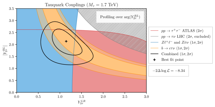
Figure 3: Preferred parameter space region providing an explanation for the $R_{D^{(*)}}$ anomalies (orange), shown in the $Y^{LR}_{3\tau}$–$Y^{RL}_{2\tau}$ plane. Our results assume that $Y^{LR}_{3\tau}$ is real and we profile over the phase of $Y^{RL}_{2\tau}$. We overlay to this contour the region favoured by $Z\tau^{+}\tau^{-}$ and $Z\bar{\nu}\nu$ data (blue), as well as that favoured by the di-tau ATLAS DY analysis (red) and that excluded by the mono-tau search (hatched). Our results exhibit a mild tension.

4.1 Tauquark

As pointed out in Ref. Angelescu:2021lln , we can explain the $R_{D}$ and $R_{D^{*}}$ anomalies with the product of couplings $Y^{LR*}_{3\tau}Y^{RL}_{2\tau}$, given the presence of a large complex phase. This phase avoids interference with the SM, at the price that the couplings need to be large and the LQ mass needs to be low. We thus set $M_{\tau}=1.7$ TeV, which is compatible with the limits originating from LQ pair production given in Table 1. In fact, such a choice leads to a LQ pair-production cross section that is a factor 4 smaller than the corresponding bound. At the same time, a non-zero $Y^{LR}_{3\tau}$ value leads to an $m_{t}^{2}/m_{Z}^{2}$ enhancement in the $Z\tau^{+}\tau^{-}$ and $Z\bar{\nu}\nu$ couplings, and our non-zero $Y^{LR}_{2\tau}$ value contributes significantly, due to the second generation quarks involved, to non-resonant $pp\to\tau^{+}\tau^{-}$ and $pp\to\tau\nu$ production.

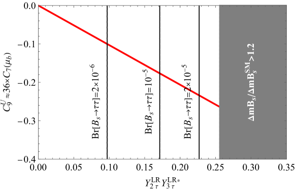
Figure 4: $\mathcal{C}_{9}^{U}\approx 36\times\mathcal{C}_{7}(\mu_{b})$ as a function of $Y^{LR}_{2\tau}Y^{LR*}_{3\tau}$ for $M_{\tau}=1.7$ TeV. The contour lines indicate predicted values for the $B_{s}\to\tau^{+}\tau^{-}$ branching ratio, and in the grey region the effect in $B_{s}-\bar{B}_{s}$ mixing is higher than 20% of the SM predictions.

We display in Figure 3 the preferred parameter space region that provides an explanation for the $R_{D^{(*)}}$ anomalies (orange), the results being projected in the $Y_{3\tau}^{LR}$–$Y_{2\tau}^{RL}$ plane. As can be seen, this leads to strong bounds on the size of the tauquark couplings to fermions. In order to derive those constraints, we have profiled over the relative complex phase of the $Y^{LR*}_{3\tau}$ and $Y^{RL}_{2\tau}$ couplings, which we attribute to $Y^{RL}_{2\tau}$ (i.e. we assume that $Y_{3\tau}^{LR}$ is real). Despite of this new source of CP violation, EDM bounds are not (yet) constraining (see Appendix C). The figure also shows the parameter space region favoured by $Z\to\tau^{+}\tau^{-}$ and $Z\to\bar{\nu}\nu$ coupling data (blue) as well as by neutral-current and charged-current DY measurements at the LHC in the di-tau (red) and mono-tau (hatched) channel. While the $R_{D^{(*)}}$ anomalies can be partially explained, there is a mild tension with the EW fit (i.e. with $Z\to\tau^{+}\tau^{-}$ and $Z\to\bar{\nu}\nu$ data), and the DY di-tau bounds derived from recent measurements achieved by the ATLAS collaboration. This leads to a combined likelihood difference

$$-2\Delta\log\mathcal{L}\equiv 2\log\mathcal{L}_{\text{SM}}-2\log\mathcal{L}=-8.34\,,$$ (59)

which corresponds to a pull of $2.1\sigma$ for three degrees of freedom (d.o.f.).

As calculated in Section 3.2, the loop-diagrams in Figure 1 induce lepton flavour violation universal effects in $b\to s\ell^{+}\ell^{-}$ decays (via ${\cal O}_{9}^{U}$ and ${\cal O}_{7}$ operators) that are proportional to the product of couplings $Y^{LR}_{2\tau}Y^{LR*}_{3\tau}$. While these contributions cannot account for the $R_{K^{(*)}}$ anomalies, they are capable of explaining (partially) $P_{5}^{\prime}$ and $B_{s}\to\phi\mu^{+}\mu^{-}$ data. Moreover, as shown in the next subsection, this effect further improves the fit to $b\to s\ell^{+}\ell^{-}$ data once the LFUV effects originating from the presence of the muoquark are included. On the other hand, the size of $Y^{LR}_{2\tau}Y^{LR*}_{3\tau}$ is limited by $B_{s}-\bar{B}_{s}$ mixing. While $Y^{LR*}_{3\tau}$ was already constrained by $Z\tau^{+}\tau-$ and $Z\bar{\nu}\nu$ data (see above), a non-zero value of $Y^{LR}_{2\tau}$ additionally contributes to $D^{0}-\bar{D}^{0}$ mixing. However, for $|Y^{LR}_{2\tau}|\approx 1/2Y^{LR*}_{3\tau}$, $B_{s}-\bar{B}_{s}$ mixing provides the leading constraint and the corresponding bounds, together with their impact on the Wilson coefficients $\mathcal{C}_{9}^{U}$ and $\mathcal{C}_{7}$ are shown in Figure 4.

4.2 Muoquark

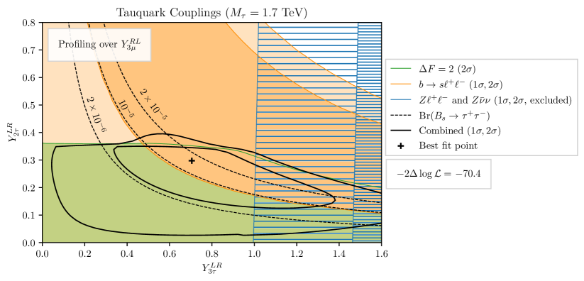
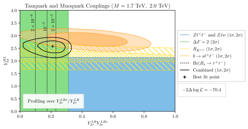
Figure 5: Top: Bounds on the $\Phi_{2,\tau}$ couplings $Y^{LR}_{3\tau}$ and $Y^{LR}_{2\tau}$ derived from the combined fit of $\Phi_{2,\tau}$ and $\Phi_{2,\mu}$ effects to $b\to s\ell^{+}\ell^{-}$ observables (orange). Our results are obtained by profiling over the $\Phi_{2,\mu}$ contributions depending on the $Y^{RL}_{3\mu}$ coupling. The coupling $Y_{2\tau}^{LR}$ is tightly constrained by $D^{0}-\bar{D}^{0}$ mixing (green), and large $Y^{LR}_{3\tau}$ values worsen the fit to $B_{s}-\bar{B}_{s}$ mixing (green as well) and leads to tension with $Z\ell^{+}\ell^{-}$ and $Z\bar{\nu}\nu$ data (blue). The figure also includes predictions for the $B_{s}\to\tau^{+}\tau^{-}$ branching ratio. Bottom: The same solution presented in terms of the product $Y^{LR}_{2\tau}Y^{LR*}_{3\tau}$ and the muoquark coupling $Y^{RL}_{3\mu}$. We profile over the ratio $Y^{LR*}_{3\tau}/Y^{LR}_{2\tau}$ that is relevant for the bounds originating from $D^{0}-\bar{D}^{0}$ mixing, as well as from the fit to $Z\tau^{+}\tau^{-}$ and $Z\bar{\nu}\nu$ data.

Regarding $b\to s\ell^{+}\ell^{-}$, an excellent fit to data can be obtained in new physics scenarios featuring an LFU $\mathcal{C}_{9}^{U}$ effect in addition to a LFUV violating effect $\mathcal{C}_{9}^{\mu}=-\mathcal{C}_{10}^{\mu}$ Alguero:2018nvb ; Alguero:2019ptt . In fact, this scenario even constitutes the two-dimensional one which gives the best fit to data Alguero:2021anc . This is precisely the setup realised in the considered model with three generations of LQs, in which the photon penguin contribution induced by the presence of the tauquark is combined with the $W$-box contribution involving the muoquark, so that $\mathcal{C}^{\mu}_{9}=-\mathcal{C}^{\mu}_{10}$. We checked that the tree-level effect giving rise to $\mathcal{C}_{9}^{\mu}=+\mathcal{C}_{10}^{\mu}$ does not improve the fit, such that $Y^{LR*}_{3\mu}Y^{LR}_{2\mu}$ must be small. Furthermore, also the preferred value of $\mathcal{C}_{9}^{e}=+\mathcal{C}_{10}^{e}$ that is induced by the electroquark is consistent with zero once added to the other LQ contributions. As before, we choose the muoquark mass to be as low as possible while still satisfying the limits from LQ pair-production searches at the LHC by a clear margin. We hence fix $M_{\mu}=2$ TeV.

In Figure 5 we focus on the three couplings $Y^{LR}_{3\tau}$, $Y^{LR}_{2\tau}$ and $Y^{RL}_{3\mu}$ of the tauquark $\Phi_{2,\tau}$ and the muoquark $\Phi_{2,\mu}$, assuming them to be real. While these couplings are constrained by $B_{s}-\bar{B}_{s}$ mixing, $D^{0}-\bar{D}^{0}$ mixing, as well as by $Z\tau^{+}\tau^{-}$ and $Z\bar{\nu}\nu$ coupling measurements, we can still significantly improve the fit to $b\to s\ell^{+}\ell^{-}$ data. In fact, a likelihood value $-2\Delta\log{\cal L}=-70.4$, corresponding to a combined pull of $7.9\sigma$ for three d.o.f., can be reached. Whereas the $W$-box contribution leading to $\mathcal{C}_{9}^{\mu}=-\mathcal{C}_{10}^{\mu}$ via a $Y^{RL}_{3\mu}$ coupling is in tension with $Z\mu^{+}\mu^{-}$ and $Z\bar{\nu}\nu$ Angelescu:2021lln data, this tension is reduced once the contribution from the tauquark discussed in Section 4.1 is accounted for. Therefore, the combined effect of $\Phi_{2,\tau}$ and $\Phi_{2,\mu}$ leptoquarks does not only result in a better fit to $b\to s\ell^{+}\ell^{-}$ data, but also weakens the bounds from EW precision observables as a smaller coupling $Y^{RL}_{3\mu}$ suffices.

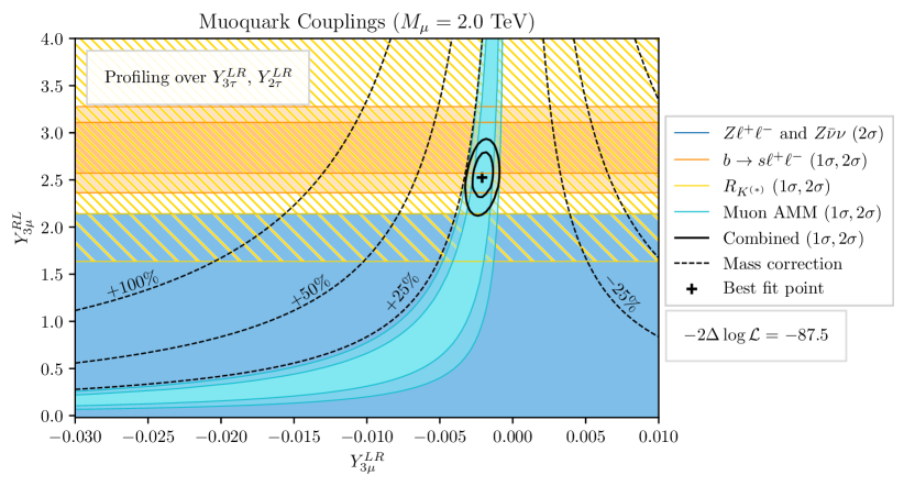
Figure 6: Simultaneous solution to the $b\to s\ell^{+}\ell^{-}$ (orange) and $\left(g-2\right)_{\mu}$ (light blue) anomalies, as obtained by combining the effects of the couplings $Y^{LR}_{3\tau}$, $Y^{LR}_{2\tau}$, $Y^{RL}_{3\mu}$ and $Y^{LR}_{3\mu}$. We additionally show the relative radiative correction to the muon mass (black lines), that are derived by only taking into account only the finite part of the involved loop function.

We now include $(g-2)_{\mu}$ in our analysis. To provide an explanation to this anomaly, we need the combined effect of non-zero $Y^{RL}_{3\mu}$ and $Y^{LR}_{3\mu}$ couplings so that we can get the desired $m_{t}/m_{\mu}$ enhancement. Adding therefore $Y^{LR}_{3\mu}$ as a free parameter, but profiling over $Y_{3\tau}^{LR}$ and $Y_{2\tau}^{LR}$, we obtain the results of Figure 6. While we have assumed that all couplings are real, they can generally be complex. As consequence, a large muon EDM can be generated Crivellin:2018qmi . Our results additionally show that a chirally enhanced explanation for the $(g-2)_{\mu}$ anomaly leads to large radiative contributions to the muon mass as well as to the $h\to\mu\mu$ branching ratio Crivellin:2021rbq . While in order to measure the latter percent-level effect a future precision determination, like at FCC-hh FCC:2018vvp , would be necessary Crivellin:2020tsz ; Crivellin:2020mjs , the contribution to the muon mass can be of order one (see the dashed isolines in Figure 6). However, this effect is not physical. It can be absorbed in a re-definition of the muon mass and thus only be bounded by fine-tuning arguments requiring the absence of large accidental cancellations. The combined log-likelihood difference is further decreased to $-87.5$, corresponding to a SM pull of $8.7\sigma$ for four d.o.f.

Finally, as shown in Ref. Carvunis:2021dss , the presence of a muoquark in the model can only weaken, but not fully explain, the anomaly in $\Delta A_{\text{FB}}$. In this case, a product of couplings $Y^{RL}_{2\mu}Y^{LR*}_{3\mu}\approx-1.4$ would lead to a pull of $1.8\sigma$ for two d.o.f. .

4.3 Electroquark

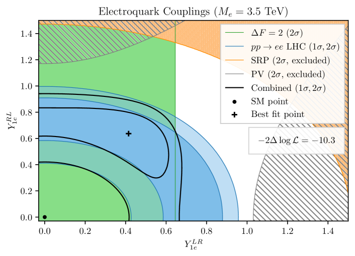
Figure 7: Parameter space region leading to a possible explanation for the excess in di-electrons found by the CMS collaboration (light blue). The solution via real couplings $Y^{LR}_{1e}$ and $Y_{1e}^{RL}$ prefers values of $\mathcal{O}(0.6)$, which also yields an improved fit to PV observables Crivellin:2021bkd . The limit from the electron EDM measurement additionally places a strong constraint on the complex phases of the couplings.

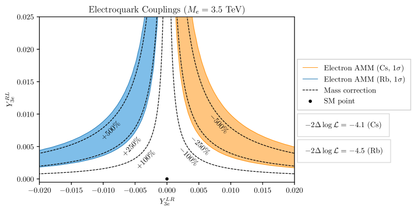
Figure 8: Potential effect of the $\Phi_{2,e}$ leptoquark on $(g-2)_{e}$ via the couplings $Y^{LR}_{3e}$ and $Y^{RL}_{3e}$. We show the preferred parameter space regions for the two contradicting SM determinations of $\left(g-2\right)_{e}$ based on Rb (blue) and Cs (orange) atoms. In the preferred parameter space regions, sizeable loop corrections to the electron mass are generated, and the EDM constraint places strong limits on the complex phases of these couplings.

In the electron sector we aim to explain the CMS excess found in non-resonant di-electron production. In order to satisfy the bounds on the electroquark mass coming from its pair production at the LHC, $M_{e}$ should be of at least 2.1 TeV. However, we also have to consider SRP limits. The latter severely restrict the electroquark couplings to light quarks, which need to be large enough to yield a sizeable effect in non-resonant di-electron production to explain the deviations considered. Importantly, SRP involves on-shell LQs, while the corresponding effect on the non-resonant di-electron spectrum occurs from $t$-channel exchange (see the diagram on the right in Figure 2). Therefore, by increasing the electroquark mass, the former bounds can be avoided independently of the LQ couplings while sizeable contributions to the latter process are still possible. We find that $M_{e}>3.5$ TeV is sufficient to avoid any SRP limits without requiring a too large Yukawa couplings when building an explanation for the non-resonant di-electron signal.

The corresponding preferred region of the parameter space is presented in the $Y^{LR}_{1e}$–$Y^{RL}_{1e}$ plane in Figure 7. Our results combine the CMS and ATLAS analyses of non-resonant di-electron production, and are shown in blue. Interestingly, these couplings can also achieve a slightly improved fit to the low-energy parity violation data Crivellin:2021bkd . Moreover, for sizeable $Y^{LR}_{1e}$ values the electron EDM limit places a strong constraint on $\text{arg}(Y^{LR}_{1e}Y^{RL*}_{1e})$. For the best-fit point in Figure 7, it has to be smaller than $\mathcal{O}(10^{-5})$.

Finally, the electroquark couplings $Y^{LR}_{3e}$ and $Y^{RL}_{3e}$ could in principle also lead to a deviation from SM predictions in $(g-2)_{e}$. The corresponding preferred regions in the parameter space are shown in Figure 8 for the two contradicting determinations of $\alpha$ considered. In this case, significant radiative corrections to the electron mass arise, which can become larger than the measured mass itself. Additionally, the same couplings can also give rise to an electron EDM, placing strong constraints on the complex phases of the involved couplings. For the best fit values for the product $Y^{LR}_{3e}Y^{RL*}_{3e}$ (i.e. at the center of the blue and orange regions in Figure 7), the complex phase needs to be $\lesssim\mathcal{O}(10^{-5})$ in order to satisfy EDM constraints.

4.4 $W$ mass

Finally, we discuss the shift in the predictions for the $W$ mass generated by the presence of LQs in our model. We show the global fit Ellis:2018gqa to new physics contributions in the Peskin-Takeuchi parameters $S$ and $T$ in Figure 9 (for one d.o.f.), together with the effects that our model can yield. The agreement with data is improved for positive values for $\Delta S$ and $\Delta T$. As an illustration, the best fit point in our model is given by

$$Y_{\ell}^{H(3)}=-1.16~{}~{}~{}(\ell=e,\mu,\tau)\,,$$ (60)

where we assume that $Y^{H(3)}_{e}=Y^{H(3)}_{\mu}=Y^{H(3)}_{\tau}$ for simplicity. The corresponding likelihood difference value is $-1.54$.

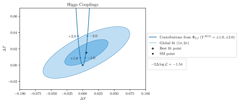
Figure 9: Global fit to the (difference of the) Peskin-Takeuchi parameters $\Delta S$ and $\Delta T$. This fit can be improved via a positive contribution to both $\Delta S$ and $\Delta T$, which corresponds to negative couplings $Y^{H(3)}_{\ell}$. We indicate the position of the points $Y^{H(3)}=\pm 1,\pm 2$ when we assume that $Y^{H(3)}_{e}=Y^{H(3)}_{\mu}=Y^{H(3)}_{\tau}\equiv Y^{H(3)}$.

5 Conclusions

While it is known that a single $SU(2)_{L}$ doublet of scalar leptoquarks can explain $b\to s\ell^{+}\ell^{-}$ data, $R_{D^{(*)}}$ and $(g-2)_{\mu}$ separately, a common explanation is not possible. This would indeed require couplings to taus, muons and electrons simultaneously, which would lead to unacceptably large effects in charged lepton flavour violating processes. In order to overcome this obstacle, we proposed in this article to extend the SM by three generations of scalar $SU(2)_{L}$ doublets $\Phi_{2,e}$, $\Phi_{2,\mu}$ and $\Phi_{2,\tau}$, each of them carrying the corresponding lepton flavour number. In that way, we can have multiple sources of LFUV while the individual lepton flavours are still exactly conserved, as in the SM (with massless neutrinos). As a result, our setup can be distinguished from LQ scenarios with a single LQ already by considering low energy observables: It predicts that while effects in observables involving different lepton generations are possible, no sign of charged lepton flavour violating should be observed. Furthermore, assigning lepton flavour numbers to LQs automatically avoids bounds from proton decay experiments, as it forbids di-quark couplings.

In this setup we showed that:

• The tauquark $\Phi_{2,\tau}$, despite effects in $Z\to\tau^{+}\tau^{-}$, $Z\to\bar{\nu}\nu$, $D^{0}-\bar{D}^{0}$ mixing and the bounds stemming from $\tau^{+}\tau^{-}$ searches at the LHC, can (mostly) explain $b\to c\tau\nu$ data in the presence of a complex phase.

• The presence of the tauquark $\Phi_{2,\tau}$ generates a universal operator ${\cal O}_{9}^{U}$ via off-shell photon penguin diagram contributions with tau leptons running in the loop. While the effect is bounded by $B_{s}-\bar{B}_{s}$ mixing and crucially depends on $M_{\tau}$ (i.e. the relative effect in $B_{s}-\bar{B}_{s}$ mixing is enhanced for larger LQ masses), a relevant contribution is possible.

• An excellent fit to $b\to s\ell^{+}\ell^{-}$ data can be obtained via a combination of tauquark contributions (generating $\mathcal{C}_{9}^{U}$) and muoquark $W$-box contribution (generating $\mathcal{C}^{\mu}_{9}=-\mathcal{C}^{\mu}_{10}$). This leads to a likelihood difference $-2\Delta\log\mathcal{L}=-70.4$, which corresponds to $7.9\sigma$ for three d.o.f. .

• $\left(g-2\right)_{\mu}$ can be explained via an $m_{t}/m_{\mu}$ enhanced muoquark contribution.

• The electron excess appearing in the invariant-mass tails of DY di-electron production at the LHC $pp\to e^{+}e^{-}$ can be accounted for via a contribution from the electroquark alone, without violating any bounds from $D^{0}-\bar{D}^{0}$ mixing.

• The EW fit can be improved by a constructive contribution to the $W$-boson mass.

• A (possible) new physics effect in $(g-2)_{e}$ could be incorporated.

For the latter, the phase of the couplings in general needs to be precisely tuned in order to avoid the bounds from electron EDM. However, this obstacle could be resolved in our model by requiring that the lepton masses are generated at the loop level Greljo:2021npi . Such a radiative mass generation leads to an automatic phase alignment between the mass term and the dipole operators such that the electron EDM vanishes Borzumati:1999sp ; Crivellin:2010gw .

Appendix A Leptoquark effects in $Z$-boson couplings

The $\Phi_{2,\ell}$ contributions $g^{\text{LQ}}_{\ell_{A}}$ to the $Z$ boson couplings to leptons are given by Crivellin:2020mjs ; Arnan:2019olv

$$\begin{split}g^{\text{LQ}}_{\ell_{L}}=&\ N_{c}\frac{Y^{RL}_{3\ell}Y^{RL*}_{3\ell}}{16\pi^{2}}\Bigg{[}\frac{x_{t,\ell}\left(x_{t,\ell}-1-\log x_{t,\ell}\right)}{2\left(x_{t,\ell}-1\right)^{2}}+\frac{x_{Z,\ell}}{12}\mathcal{G}_{L}(x_{t,\ell},g^{\text{tree}}_{\ell_{L}})\Bigg{]}\\ &\qquad+x_{Z,\ell}N_{c}\sum_{k=1,2}\frac{Y^{RL}_{k\ell}Y^{RL*}_{k\ell}}{48\pi^{2}}\Bigg{[}\frac{2s_{w}^{2}}{3}\ \left(\log x_{Z,\ell}-i\pi-\frac{1}{6}\right)+\frac{g^{\text{tree}}_{\ell_{L}}}{6}\Bigg{]}\,,\\ g^{\text{LQ}}_{\ell_{R}}=&\ N_{c}\frac{\hat{Y}^{LR}_{3\ell}\hat{Y}^{LR*}_{3\ell}}{16\pi^{2}}\Bigg{[}-\frac{x_{t,\ell}\left(x_{t,\ell}-1-\log x_{t,\ell}\right)}{2\left(x_{t,\ell}-1\right)^{2}}+\frac{x_{Z,\ell}}{12}\mathcal{G}_{R}(x_{t,\ell},g^{\text{tree}}_{\ell_{R}})\Bigg{]}\\ &\quad+x_{Z,\ell}N_{c}\sum_{k=1,2}\frac{\hat{Y}^{LR}_{k\ell}\hat{Y}^{LR*}_{k\ell}}{48\pi^{2}}\Bigg{[}\left(-\frac{1}{2}+\frac{2s_{w}^{2}}{3}\right)\left(\log x_{Z,\ell}-i\pi-\frac{1}{6}\right)+\frac{g^{\text{tree}}_{\ell_{R}}}{6}\Bigg{]}\\ &\quad+x_{Z,\ell}N_{c}\sum_{k=1,2,3}\frac{Y^{RL}_{k\ell}Y^{RL*}_{k\ell}}{48\pi^{2}}\Bigg{[}\left(\frac{1}{2}-\frac{s_{w}^{2}}{3}\right)\left(\log x_{Z,\ell}-i\pi-\frac{1}{6}\right)+\frac{g^{\text{tree}}_{\ell_{R}}}{6}\Bigg{]}\,,\end{split}$$ (61)

where $x_{t,\ell}\equiv m_{t}^{2}/M_{\ell}^{2}$, $x_{Z,\ell}\equiv m_{Z}^{2}/M_{\ell}^{2}$ and the tree-level SM couplings are $g^{\text{tree}}_{\ell_{L}}=-\frac{1}{2}+s_{w}^{2}$ and $g^{\text{tree}}_{\ell_{R}}=s_{w}^{2}$. The functions $\mathcal{G}_{L}$ and $\mathcal{G}_{R}$ contain the $\mathcal{O}\left(x_{Z}\log x_{t}\right)$ terms that induce non-negligible corrections when the LQ mass is small. They read

$$\begin{split}\mathcal{G}_{L(R)}(x,g_{\ell})=&\ g^{\text{tree}}_{u_{R(L)}}\frac{\left(x-1\right)\left(5x^{2}-7x+8\right)-2\left(x^{3}+2\right)\log x}{\left(x-1\right)^{4}}\\ &\ +g^{\text{tree}}_{u_{L(R)}}\frac{\left(x-1\right)\left(x^{2}-5x-2\right)+6x\log x}{\left(x-1\right)^{4}}\\ &\ +g_{\ell}\frac{\left(x-1\right)\left(-11x^{2}+7x-2\right)+6x^{3}\log x}{3\left(x-1\right)^{4}}\,,\end{split}$$ (62)

where $g^{\text{tree}}_{u_{L}}=\frac{1}{2}-\frac{2}{3}s_{w}^{2}$ and $g^{\text{tree}}_{u_{R}}=-\frac{2}{3}s_{w}^{2}$. The neutrino coupling $g^{\text{LQ}}_{\nu_{\ell,L}}$ can be derived from $g^{\text{LQ}}_{\ell_{L}}$ by replacing the tree-level coupling $g^{\text{tree}}_{\ell_{L}}$ by $g^{\text{tree}}_{\nu_{\ell,L}}=\frac{1}{2}$.

Appendix B Details of the LHC analyses

B.1 CMS non-resonant di-lepton production at the LHC

We determined the cross sections in Eq. (54) for each value of the couplings $Y^{LR}_{i\ell},Y^{RL}_{i\ell}\in\{0.25,0.5,1.0,2.0\}$ individually, setting the other couplings to zero. We implemented a selection on the transverse momentum and pseudo-rapidity of the electrons (muons), namely $p_{T}>35$ GeV (53 GeV) and $|\eta|<2.5$ (2.4), which allows us to mimic the lepton candidate definitions of Ref. Sirunyan:2021khd . By fitting a polynomial in the Yukawa couplings to the resulting cross sections, we determined the contributions from the SM alone, the LQs alone, and the LQ-SM interference term for LQ-fermion couplings set to one. This provides enough information to calculate the different components of the cross section for general Yukawa coupling values through a rescaling of the results.

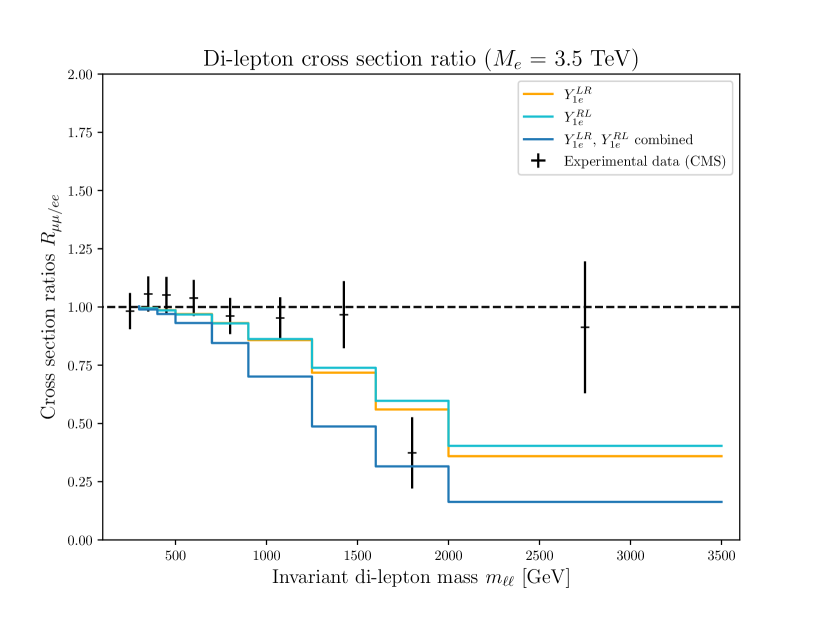
Figure 10: The resulting values $R_{\mu\mu/ee}$ in the nine di-lepton mass bins. We show the distributions for an electroquark extension of the SM with $Y^{LR}_{1e}=1.0$ and/or $Y^{RL}_{1e}=1.0$.

Based on these cross sections we derive the ratios $R^{\text{LQ+SM}}_{\mu\mu/ee,n}\big{/}R^{\text{SM}}_{\mu\mu/ee,n}$. The results for a specific scenario are shown in Figure 10, overlayed with the data from Ref. Sirunyan:2021khd . This allows us to build the likelihood function

$$-2\log\mathcal{L}=\sum_{n=1}^{9}\frac{\left(\dfrac{R_{\mu\mu/ee,n}^{\text{data}}}{R_{\mu\mu/ee,n}^{\text{MC}}}-\dfrac{R_{\mu\mu/ee,n}^{\text{SM+LQ}}}{R_{\mu\mu/ee,n}^{\text{SM}}}\right)^{2}}{\sigma_{n}^{2}}\,,$$ (63)

where $n$ runs over the nine $m_{\ell\ell}$ bins and $\sigma_{n}$ are the experimental uncertainties reported in Ref. Sirunyan:2021khd .

B.2 ATLAS non-resonant di-lepton production at the LHC

In our analysis, we estimated the individual cross sections in the SRs chosen by the ATLAS collaboration using MadGraph_aMC@NLO, analogously to the setup described in Section 3.9. We implemented lepton $p_{T}$ cuts of 30 GeV (30 GeV) and $|\eta|$ cuts of 2.47 (2.5) on electron (muon) candidates. Based on the resulting cross sections for Yukawa coupling values of one, we extracted the ratios

$$\mu_{\ell}\equiv\dfrac{\int_{\text{SR}}\frac{d\sigma^{\text{LQ+SM}}}{dm_{\ell\ell}}\left(pp\to\ell^{+}\ell^{-}\right)dm_{\ell\ell}}{\int_{\text{SR}}\frac{d\sigma^{\text{SM}}}{dm_{\ell\ell}}\left(pp\to\ell^{+}\ell^{-}\right)dm_{\ell\ell}}$$ (64)

with $\ell=e,\mu$ for general Yukawa coupling matrices $Y^{LR}$ and $Y^{RL}$. We then followed the statistical analysis achieved by the ATLAS collaboration, and built a likelihood function using a single-bin Poissonian counting-experiment approach. In the latter, the uncertainties are accounted for as Gaussian constraints that we profile over ATLAS:2020yat ; Junk:1999kv .

B.3 Non-resonant di-tau production at the LHC

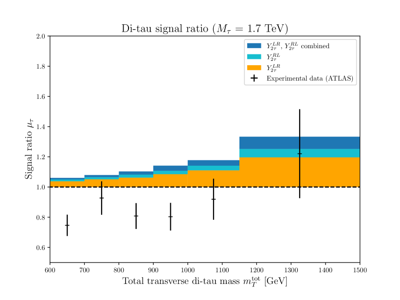
Figure 11: Signal ratios $\mu_{\tau}$ for the six $m_{T}^{\text{tot}}$ bins studied in the considered ATLAS analysis (for $m_{T}$ ranging from 600 to 1500 GeV). We show the contributions of a tauquark $\Phi_{2,\tau}$ with a mass $M_{\tau}$ = 1.7 TeV and Yukawa couplings $Y^{LR}_{2\tau}=1.5$ and $Y^{RL}_{2\tau}=1.5$. We distinguish between the contributions from $Y^{LR}_{2\tau}$ and those from $Y^{RL}_{2\tau}$, taking the two couplings individually, and include as well results for a setup with both of them included.

We focus on the production of a pair of tau leptons at the LHC when the di-tau system has a large invariant mass. We consider di-tau events populating the signal region of the ATLAS analysis of Ref. ATLAS:2020yat , and focus on the six highest bins in the total transverse mass $m_{T}^{\text{tot}}$ bins defined by

$$m_{T}^{\text{tot}}\equiv\sqrt{\left(p_{T}^{\tau_{1}}+p_{T}^{\tau_{2}}+E_{T}^{\text{miss}}\right)^{2}-\left(\mathbf{p}_{T}^{\tau_{1}}+\mathbf{p}_{T}^{\tau_{1}}+\mathbf{E}_{T}^{\text{miss}}\right)^{2}}\,.$$ (65)

In this expression, $\mathbf{p}_{T}^{\tau_{1}}$ and $\mathbf{p}_{T}^{\tau_{2}}$ are the transverse momenta of the visible daughter particles originating from the two hadronically-decaying taus, and $\mathbf{E}_{T}^{\text{miss}}$ is the total missing transverse momentum vector stemming from the unresolved particles including the daughter neutrinos. In our notation, $p_{T}^{\tau_{1}}$, $p_{T}^{\tau_{2}}$ and $E_{T}^{\text{miss}}$ are the respective moduli of the different two-vectors. The corresponding measurements are shown in Figure 11 for $m_{T}^{\rm tot}$ bins defined by endpoints in $\{600,700,800,900,1000,1150,1500\}$ GeV.

In our analysis, we generated partonic $pp\to\tau^{+}\tau^{-}$ events using MadGraph_aMC@NLO, analogously to what has been done in Section 3.9 but with loose cuts on the tau leptons ($p_{T}>65$ GeV, $\left|\eta\right|<2.5$) and on the invariant mass of the di-tau system $m_{\tau\tau}>200$ GeV. We then showered these events with Pythia version 8.306 Sjostrand:2014zea and analysed the resulting hadronic events using MadAnalysis 5 Conte:2012fm ; Conte:2014zja ; Conte:2018vmg and a FastJet-based detector simulation Cacciari:2011ma ; Araz:2020lnp . At the reconstructed level, we imposed $p_{T}>160$ GeV and $|\eta|<2.5$ for each hadronic tau and finally carried out the binning in $m_{T}^{\text{tot}}$.

This yielded

$$\mu_{\tau,n}\equiv\dfrac{\int_{\text{bin n}}\frac{d\sigma^{\text{LQ+SM}}}{dm^{\text{tot}}_{T}}\left(pp\to\tau_{\text{had}}^{+}\tau_{\text{had}}^{-}\right)dm^{\text{tot}}_{T}}{\int_{\text{bin n}}\frac{d\sigma^{\text{SM}}}{dm^{\text{tot}}_{T}}\left(pp\to\tau_{\text{had}}^{+}\tau_{\text{had}}^{-}\right)dm^{\text{tot}}_{T}}\times R_{n}\,,$$ (66)

for the $n=1,\dots,6$ bins indicated above, and for general Yukawa coupling matrices $Y^{LR}$ and $Y^{RL}$. The factor $R_{n}\in[0,1]$ accounts for the additional SM backgrounds originating from multijet production and the charged-current process $pp\to W\to\tau\nu$ that are small but not negligible compared to the background from the Drell-Yan process $pp\to(Z/\gamma)^{\ast}\to\tau^{+}\tau^{-}$ ATLAS:2020zms . The resulting signal ratios for a specific scenario are given in Figure 11. Finally, we again built a likelihood using a multi-bin Poissonian counting-experiment approach with Gaussian constraints for the uncertainties.

Appendix C Electric dipole moments of hadrons

	Coupling
	$X_{12}$	$X_{22}$	$X_{13}$	$X_{23}$
Fundamental limits	$<9\times 10^{-4}$	–	$<7\times 10^{-5}$	–
Measurement	$d_{n}$	–	$d_{n}$	–
Strict limits	$4\times 10^{-4}$	0.5 (3)	$3\times 10^{-5}$	$3\times 10^{-2}(0.2)$
Measurement	$d_{\text{Hg}}$	$d_{\text{Hg}}$	$d_{\text{Hg}}$	$d_{\text{Hg}}$

Table 2: Limits on the LQ couplings to fermions coming from EDM measurements in hadrons. We only show the constraints that are more stringent than the ones originating from lepton EDM measurements.

The experiments targeting the observation of EDMs in neutrons Pendlebury:2015lrz ; Baker:2006ts ; nEDM:2020crw and Hg atoms Griffith:2009zz ; Graner:2016ses have so far yielded null results. For our model, the most relevant resulting upper limits (at 90% C.L.) are given by

$$d_{n} <1.8\times 10^{-26}\text{e cm}\qquad\text{and}\qquad d_{\text{Hg}} <6.3\times 10^{-30}\text{e cm}\,.$$ (67)

Ref. Dekens:2018bci presented a detailed study of the LQ effects in the EDMs of hadrons. In Table 2 we list the subset of their limits that are more stringent than the ones coming from the lepton EDMs, extracting the bounds on the quantity

$$X_{i\ell}\equiv\text{Im}\left[\frac{\hat{Y}^{LR}_{i\ell}Y^{RL*}_{i\ell}}{M_{\ell}^{2}}\right]\,,$$ (68)

for $i,\ell=1,2,3$. The authors of Ref. Dekens:2018bci presented two sets of limits. The first one is based on a “pessimistic” approach (fundamental limits), where all matrix elements are varied within their admissible theoretical ranges without assuming any probability distribution. This method is called the range-fit method that is suitable to rule out models. The second set of limits is based on a more “optimistic” approach (strict limits), where the theoretical uncertainties are neglected and the central values of the hadronic, nuclear, and atomic matrix elements are assumed to be true. The real constraints are likely to lie between these two extremes. The table additionally includes, in parentheses, the limits that can be obtained after neglecting the contributions from charm tensor charge.

Whereas the strictest limit for $X_{23}$ in Table 2 would rule out the $\Phi_{2,\tau}$ solution to $R_{D^{(*)}}$, the authors of Ref. Dekens:2018bci noted that due to the large theoretical uncertainties inherent to the derivation of this limit it is too early to draw strong conclusions regarding the viability of the $\Phi_{2,\tau}$ solution. It will however be interesting to see whether next-generation $d_{n}$ or $d_{\text{Hg}}$ experiments will be able to detect EDM signals.

- (1) ATLAS collaboration, Observation of a new particle in the search for the Standard Model Higgs boson with the ATLAS detector at the LHC, Phys. Lett. B 716 (2012) 1 [1207.7214].
- (2) CMS collaboration, Observation of a New Boson at a Mass of 125 GeV with the CMS Experiment at the LHC, Phys. Lett. B 716 (2012) 30 [1207.7235].
- (3) O. Fischer et al., Unveiling Hidden Physics at the LHC, 2109.06065.
- (4) A. Crivellin and M. Hoferichter, Hints of lepton flavor universality violations, Science 374 (2021) 1051 [2111.12739].
- (5) CMS, LHCb collaboration, Observation of the rare decay from the combined analysis of CMS and LHCb data, Nature 522 (2015) 68 [1411.4413].
- (6) LHCb collaboration, Angular analysis of the decay using 3 fb-1 of integrated luminosity, JHEP 02 (2016) 104 [1512.04442].
- (7) Belle collaboration, Angular analysis of , in LHC Ski 2016: A First Discussion of 13 TeV Results, 4, 2016 [1604.04042].
- (8) LHCb collaboration, Test of lepton universality with decays, JHEP 08 (2017) 055 [1705.05802].
- (9) LHCb collaboration, Search for lepton-universality violation in decays, Phys. Rev. Lett. 122 (2019) 191801 [1903.09252].
- (10) LHCb collaboration, Measurement of -Averaged Observables in the Decay, Phys. Rev. Lett. 125 (2020) 011802 [2003.04831].
- (11) LHCb collaboration, Test of lepton universality in beauty-quark decays, 2103.11769.
- (12) BELLE collaboration, Test of lepton flavor universality and search for lepton flavor violation in decays, JHEP 03 (2021) 105 [1908.01848].
- (13) Belle collaboration, Test of Lepton-Flavor Universality in Decays at Belle, Phys. Rev. Lett. 126 (2021) 161801 [1904.02440].
- (14) LHCb collaboration, Measurements of the S-wave fraction in decays and the differential branching fraction, JHEP 11 (2016) 047 [1606.04731].
- (15) LHCb collaboration, Branching Fraction Measurements of the Rare and - Decays, Phys. Rev. Lett. 127 (2021) 151801 [2105.14007].
- (16) LHCb, ATLAS, CMS collaboration, Combination of the ATLAS, CMS and LHCb results on the decays, .
- (17) BaBar collaboration, Evidence for an excess of decays, Phys. Rev. Lett. 109 (2012) 101802 [1205.5442].
- (18) BaBar collaboration, Measurement of an Excess of Decays and Implications for Charged Higgs Bosons, Phys. Rev. D 88 (2013) 072012 [1303.0571].
- (19) LHCb collaboration, Measurement of the ratio of branching fractions , Phys. Rev. Lett. 115 (2015) 111803 [1506.08614].
- (20) LHCb collaboration, Test of Lepton Flavor Universality by the measurement of the branching fraction using three-prong decays, Phys. Rev. D 97 (2018) 072013 [1711.02505].
- (21) LHCb collaboration, Measurement of the ratio of the and branching fractions using three-prong -lepton decays, Phys. Rev. Lett. 120 (2018) 171802 [1708.08856].
- (22) Belle collaboration, Measurement of and with a semileptonic tagging method, 1904.08794.
- (23) W. Altmannshofer and P. Stangl, New physics in rare B decays after Moriond 2021, Eur. Phys. J. C 81 (2021) 952 [2103.13370].
- (24) L.-S. Geng, B. Grinstein, S. Jäger, S.-Y. Li, J. Martin Camalich and R.-X. Shi, Implications of new evidence for lepton-universality violation in b→s+- decays, Phys. Rev. D 104 (2021) 035029 [2103.12738].
- (25) M. Algueró, B. Capdevila, S. Descotes-Genon, J. Matias and M. Novoa-Brunet, Global Fits after and , 4, 2021 [2104.08921].
- (26) T. Hurth, F. Mahmoudi, D.M. Santos and S. Neshatpour, More indications for lepton nonuniversality in , Phys. Lett. B 824 (2022) 136838 [2104.10058].
- (27) K. Kowalska, D. Kumar and E.M. Sessolo, Implications for new physics in transitions after recent measurements by Belle and LHCb, Eur. Phys. J. C 79 (2019) 840 [1903.10932].
- (28) M. Ciuchini, M. Fedele, E. Franco, A. Paul, L. Silvestrini and M. Valli, New Physics without bias: Charming Penguins and Lepton Universality Violation in decays, 2110.10126.
- (29) G. D’Amico, M. Nardecchia, P. Panci, F. Sannino, A. Strumia, R. Torre et al., Flavour anomalies after the measurement, JHEP 09 (2017) 010 [1704.05438].
- (30) A. Arbey, T. Hurth, F. Mahmoudi, D.M. Santos and S. Neshatpour, Update on the b→s anomalies, Phys. Rev. D 100 (2019) 015045 [1904.08399].
- (31) D. Kumar, K. Kowalska and E.M. Sessolo, Global Bayesian Analysis of new physics in transitions after Moriond-2019, in 17th Conference on Flavor Physics and CP Violation, 6, 2019 [1906.08596].
- (32) G. Isidori, D. Lancierini, P. Owen and N. Serra, On the significance of new physics in decays, Phys. Lett. B 822 (2021) 136644 [2104.05631].
- (33) HFLAV collaboration, Averages of b-hadron, c-hadron, and -lepton properties as of 2018, Eur. Phys. J. C 81 (2021) 226 [1909.12524].
- (34) Muon g-2 collaboration, Final Report of the Muon E821 Anomalous Magnetic Moment Measurement at BNL, Phys. Rev. D 73 (2006) 072003 [hep-ex/0602035].
- (35) Muon g-2 collaboration, Measurement of the Positive Muon Anomalous Magnetic Moment to 0.46 ppm, Phys. Rev. Lett. 126 (2021) 141801 [2104.03281].
- (36) T. Aoyama et al., The anomalous magnetic moment of the muon in the Standard Model, Phys. Rept. 887 (2020) 1 [2006.04822].
- (37) T. Aoyama, M. Hayakawa, T. Kinoshita and M. Nio, Complete Tenth-Order QED Contribution to the Muon g-2, Phys. Rev. Lett. 109 (2012) 111808 [1205.5370].
- (38) T. Aoyama, T. Kinoshita and M. Nio, Theory of the Anomalous Magnetic Moment of the Electron, Atoms 7 (2019) 28.
- (39) A. Czarnecki, W.J. Marciano and A. Vainshtein, Refinements in electroweak contributions to the muon anomalous magnetic moment, Phys. Rev. D 67 (2003) 073006 [hep-ph/0212229].
- (40) C. Gnendiger, D. Stöckinger and H. Stöckinger-Kim, The electroweak contributions to after the Higgs boson mass measurement, Phys. Rev. D 88 (2013) 053005 [1306.5546].
- (41) M. Davier, A. Hoecker, B. Malaescu and Z. Zhang, Reevaluation of the hadronic vacuum polarisation contributions to the Standard Model predictions of the muon and using newest hadronic cross-section data, Eur. Phys. J. C 77 (2017) 827 [1706.09436].
- (42) A. Keshavarzi, D. Nomura and T. Teubner, Muon and : a new data-based analysis, Phys. Rev. D 97 (2018) 114025 [1802.02995].
- (43) G. Colangelo, M. Hoferichter and P. Stoffer, Two-pion contribution to hadronic vacuum polarization, JHEP 02 (2019) 006 [1810.00007].
- (44) M. Hoferichter, B.-L. Hoid and B. Kubis, Three-pion contribution to hadronic vacuum polarization, JHEP 08 (2019) 137 [1907.01556].
- (45) M. Davier, A. Hoecker, B. Malaescu and Z. Zhang, A new evaluation of the hadronic vacuum polarisation contributions to the muon anomalous magnetic moment and to , Eur. Phys. J. C 80 (2020) 241 [1908.00921].
- (46) A. Keshavarzi, D. Nomura and T. Teubner, of charged leptons, , and the hyperfine splitting of muonium, Phys. Rev. D 101 (2020) 014029 [1911.00367].
- (47) A. Kurz, T. Liu, P. Marquard and M. Steinhauser, Hadronic contribution to the muon anomalous magnetic moment to next-to-next-to-leading order, Phys. Lett. B 734 (2014) 144 [1403.6400].
- (48) K. Melnikov and A. Vainshtein, Hadronic light-by-light scattering contribution to the muon anomalous magnetic moment revisited, Phys. Rev. D 70 (2004) 113006 [hep-ph/0312226].
- (49) P. Masjuan and P. Sanchez-Puertas, Pseudoscalar-pole contribution to the : a rational approach, Phys. Rev. D 95 (2017) 054026 [1701.05829].
- (50) G. Colangelo, M. Hoferichter, M. Procura and P. Stoffer, Dispersion relation for hadronic light-by-light scattering: two-pion contributions, JHEP 04 (2017) 161 [1702.07347].
- (51) M. Hoferichter, B.-L. Hoid, B. Kubis, S. Leupold and S.P. Schneider, Dispersion relation for hadronic light-by-light scattering: pion pole, JHEP 10 (2018) 141 [1808.04823].
- (52) A. Gérardin, H.B. Meyer and A. Nyffeler, Lattice calculation of the pion transition form factor with Wilson quarks, Phys. Rev. D 100 (2019) 034520 [1903.09471].
- (53) J. Bijnens, N. Hermansson-Truedsson and A. Rodríguez-Sánchez, Short-distance constraints for the HLbL contribution to the muon anomalous magnetic moment, Phys. Lett. B 798 (2019) 134994 [1908.03331].
- (54) G. Colangelo, F. Hagelstein, M. Hoferichter, L. Laub and P. Stoffer, Longitudinal short-distance constraints for the hadronic light-by-light contribution to with large- Regge models, JHEP 03 (2020) 101 [1910.13432].
- (55) T. Blum, N. Christ, M. Hayakawa, T. Izubuchi, L. Jin, C. Jung et al., Hadronic Light-by-Light Scattering Contribution to the Muon Anomalous Magnetic Moment from Lattice QCD, Phys. Rev. Lett. 124 (2020) 132002 [1911.08123].
- (56) G. Colangelo, M. Hoferichter, A. Nyffeler, M. Passera and P. Stoffer, Remarks on higher-order hadronic corrections to the muon g2, Phys. Lett. B 735 (2014) 90 [1403.7512].
- (57) S. Borsanyi et al., Leading hadronic contribution to the muon magnetic moment from lattice QCD, Nature 593 (2021) 51 [2002.12347].
- (58) M. Passera, W.J. Marciano and A. Sirlin, The Muon g-2 and the bounds on the Higgs boson mass, Phys. Rev. D 78 (2008) 013009 [0804.1142].
- (59) J. Haller, A. Hoecker, R. Kogler, K. Mönig, T. Peiffer and J. Stelzer, Update of the global electroweak fit and constraints on two-Higgs-doublet models, Eur. Phys. J. C 78 (2018) 675 [1803.01853].
- (60) A. Crivellin, M. Hoferichter, C.A. Manzari and M. Montull, Hadronic Vacuum Polarization: versus Global Electroweak Fits, Phys. Rev. Lett. 125 (2020) 091801 [2003.04886].
- (61) A. Keshavarzi, W.J. Marciano, M. Passera and A. Sirlin, Muon and connection, Phys. Rev. D 102 (2020) 033002 [2006.12666].
- (62) J.C. Pati and A. Salam, Lepton Number as the Fourth Color, Phys. Rev. D 10 (1974) 275.
- (63) H. Georgi and S.L. Glashow, Unity of All Elementary Particle Forces, Phys. Rev. Lett. 32 (1974) 438.
- (64) S. Dimopoulos, S. Raby and L. Susskind, Light Composite Fermions, Nucl. Phys. B 173 (1980) 208.
- (65) G. Senjanovic and A. Sokorac, Light Leptoquarks in SO(10), Z. Phys. C 20 (1983) 255.
- (66) P.H. Frampton and B.-H. Lee, SU(15) GRAND UNIFICATION, Phys. Rev. Lett. 64 (1990) 619.
- (67) E. Witten, Symmetry Breaking Patterns in Superstring Models, Nucl. Phys. B 258 (1985) 75.
- (68) R. Alonso, B. Grinstein and J. Martin Camalich, Lepton universality violation and lepton flavor conservation in -meson decays, JHEP 10 (2015) 184 [1505.05164].
- (69) L. Calibbi, A. Crivellin and T. Ota, Effective Field Theory Approach to , and with Third Generation Couplings, Phys. Rev. Lett. 115 (2015) 181801 [1506.02661].
- (70) G. Hiller, D. Loose and K. Schönwald, Leptoquark Flavor Patterns & B Decay Anomalies, JHEP 12 (2016) 027 [1609.08895].
- (71) B. Bhattacharya, A. Datta, J.-P. Guévin, D. London and R. Watanabe, Simultaneous Explanation of the and Puzzles: a Model Analysis, JHEP 01 (2017) 015 [1609.09078].
- (72) D. Buttazzo, A. Greljo, G. Isidori and D. Marzocca, B-physics anomalies: a guide to combined explanations, JHEP 11 (2017) 044 [1706.07808].
- (73) R. Barbieri, G. Isidori, A. Pattori and F. Senia, Anomalies in -decays and flavour symmetry, Eur. Phys. J. C 76 (2016) 67 [1512.01560].
- (74) R. Barbieri, C.W. Murphy and F. Senia, B-decay Anomalies in a Composite Leptoquark Model, Eur. Phys. J. C 77 (2017) 8 [1611.04930].
- (75) L. Calibbi, A. Crivellin and T. Li, Model of vector leptoquarks in view of the -physics anomalies, Phys. Rev. D 98 (2018) 115002 [1709.00692].
- (76) A. Crivellin, D. Müller, A. Signer and Y. Ulrich, Correlating lepton flavor universality violation in decays with using leptoquarks, Phys. Rev. D 97 (2018) 015019 [1706.08511].
- (77) M. Bordone, C. Cornella, J. Fuentes-Martín and G. Isidori, Low-energy signatures of the model: from -physics anomalies to LFV, JHEP 10 (2018) 148 [1805.09328].
- (78) J. Kumar, D. London and R. Watanabe, Combined Explanations of the and Anomalies: a General Model Analysis, Phys. Rev. D 99 (2019) 015007 [1806.07403].
- (79) A. Crivellin, C. Greub, D. Müller and F. Saturnino, Importance of Loop Effects in Explaining the Accumulated Evidence for New Physics in B Decays with a Vector Leptoquark, Phys. Rev. Lett. 122 (2019) 011805 [1807.02068].
- (80) A. Crivellin and F. Saturnino, Explaining the Flavor Anomalies with a Vector Leptoquark (Moriond 2019 update), PoS DIS2019 (2019) 163 [1906.01222].
- (81) C. Cornella, J. Fuentes-Martin and G. Isidori, Revisiting the vector leptoquark explanation of the B-physics anomalies, JHEP 07 (2019) 168 [1903.11517].
- (82) M. Bordone, O. Catà and T. Feldmann, Effective Theory Approach to New Physics with Flavour: General Framework and a Leptoquark Example, JHEP 01 (2020) 067 [1910.02641].
- (83) J. Bernigaud, I. de Medeiros Varzielas and J. Talbert, Finite Family Groups for Fermionic and Leptoquark Mixing Patterns, JHEP 01 (2020) 194 [1906.11270].
- (84) J. Aebischer, A. Crivellin and C. Greub, QCD improved matching for semileptonic B decays with leptoquarks, Phys. Rev. D 99 (2019) 055002 [1811.08907].
- (85) J. Fuentes-Martín, G. Isidori, M. König and N. Selimović, Vector Leptoquarks Beyond Tree Level, Phys. Rev. D 101 (2020) 035024 [1910.13474].
- (86) O. Popov, M.A. Schmidt and G. White, as a single leptoquark solution to and , Phys. Rev. D 100 (2019) 035028 [1905.06339].
- (87) S. Fajfer and N. Košnik, Vector leptoquark resolution of and puzzles, Phys. Lett. B 755 (2016) 270 [1511.06024].
- (88) M. Blanke and A. Crivellin, Meson Anomalies in a Pati-Salam Model within the Randall-Sundrum Background, Phys. Rev. Lett. 121 (2018) 011801 [1801.07256].
- (89) I. de Medeiros Varzielas and J. Talbert, Simplified Models of Flavourful Leptoquarks, Eur. Phys. J. C 79 (2019) 536 [1901.10484].
- (90) I. de Medeiros Varzielas and G. Hiller, Clues for flavor from rare lepton and quark decays, JHEP 06 (2015) 072 [1503.01084].
- (91) A. Crivellin, D. Müller and F. Saturnino, Flavor Phenomenology of the Leptoquark Singlet-Triplet Model, JHEP 06 (2020) 020 [1912.04224].
- (92) S. Saad, Combined explanations of , , anomalies in a two-loop radiative neutrino mass model, Phys. Rev. D 102 (2020) 015019 [2005.04352].
- (93) S. Saad and A. Thapa, Common origin of neutrino masses and , anomalies, Phys. Rev. D 102 (2020) 015014 [2004.07880].
- (94) V. Gherardi, D. Marzocca and E. Venturini, Low-energy phenomenology of scalar leptoquarks at one-loop accuracy, JHEP 01 (2021) 138 [2008.09548].
- (95) L. Da Rold and F. Lamagna, Model for the singlet-triplet leptoquarks, Phys. Rev. D 103 (2021) 115007 [2011.10061].
- (96) A. Greljo, P. Stangl and A.E. Thomsen, A model of muon anomalies, Phys. Lett. B 820 (2021) 136554 [2103.13991].
- (97) M. Bordone, C. Cornella, J. Fuentes-Martin and G. Isidori, A three-site gauge model for flavor hierarchies and flavor anomalies, Phys. Lett. B 779 (2018) 317 [1712.01368].
- (98) A. Biswas, D. Kumar Ghosh, N. Ghosh, A. Shaw and A.K. Swain, Collider signature of Leptoquark and constraints from observables, J. Phys. G 47 (2020) 045005 [1808.04169].
- (99) J. Heeck and D. Teresi, Pati-Salam explanations of the B-meson anomalies, JHEP 12 (2018) 103 [1808.07492].
- (100) S. Sahoo and R. Mohanta, Scalar leptoquarks and the rare meson decays, Phys. Rev. D 91 (2015) 094019 [1501.05193].
- (101) C.-H. Chen, T. Nomura and H. Okada, Explanation of and muon , and implications at the LHC, Phys. Rev. D 94 (2016) 115005 [1607.04857].
- (102) U.K. Dey, D. Kar, M. Mitra, M. Spannowsky and A.C. Vincent, Searching for Leptoquarks at IceCube and the LHC, Phys. Rev. D 98 (2018) 035014 [1709.02009].
- (103) D. Bečirević and O. Sumensari, A leptoquark model to accommodate and , JHEP 08 (2017) 104 [1704.05835].
- (104) B. Chauhan, B. Kindra and A. Narang, Discrepancies in simultaneous explanation of flavor anomalies and IceCube PeV events using leptoquarks, Phys. Rev. D 97 (2018) 095007 [1706.04598].
- (105) D. Bečirević, I. Doršner, S. Fajfer, N. Košnik, D.A. Faroughy and O. Sumensari, Scalar leptoquarks from grand unified theories to accommodate the -physics anomalies, Phys. Rev. D 98 (2018) 055003 [1806.05689].
- (106) S. Fajfer, J.F. Kamenik, I. Nisandzic and J. Zupan, Implications of Lepton Flavor Universality Violations in B Decays, Phys. Rev. Lett. 109 (2012) 161801 [1206.1872].
- (107) N.G. Deshpande and A. Menon, Hints of R-parity violation in B decays into , JHEP 01 (2013) 025 [1208.4134].
- (108) M. Freytsis, Z. Ligeti and J.T. Ruderman, Flavor models for , Phys. Rev. D 92 (2015) 054018 [1506.08896].
- (109) M. Bauer and M. Neubert, Minimal Leptoquark Explanation for the , , and Anomalies, Phys. Rev. Lett. 116 (2016) 141802 [1511.01900].
- (110) X.-Q. Li, Y.-D. Yang and X. Zhang, Revisiting the one leptoquark solution to the R(D(∗)) anomalies and its phenomenological implications, JHEP 08 (2016) 054 [1605.09308].
- (111) J. Zhu, H.-M. Gan, R.-M. Wang, Y.-Y. Fan, Q. Chang and Y.-G. Xu, Probing the R-parity violating supersymmetric effects in the exclusive decays, Phys. Rev. D 93 (2016) 094023 [1602.06491].
- (112) O. Popov and G.A. White, One Leptoquark to unify them? Neutrino masses and unification in the light of , and anomalies, Nucl. Phys. B 923 (2017) 324 [1611.04566].
- (113) N.G. Deshpande and X.-G. He, Consequences of R-parity violating interactions for anomalies in and , Eur. Phys. J. C 77 (2017) 134 [1608.04817].
- (114) D. Bečirević, N. Košnik, O. Sumensari and R. Zukanovich Funchal, Palatable Leptoquark Scenarios for Lepton Flavor Violation in Exclusive modes, JHEP 11 (2016) 035 [1608.07583].
- (115) Y. Cai, J. Gargalionis, M.A. Schmidt and R.R. Volkas, Reconsidering the One Leptoquark solution: flavor anomalies and neutrino mass, JHEP 10 (2017) 047 [1704.05849].
- (116) W. Altmannshofer, P.S. Bhupal Dev and A. Soni, anomaly: A possible hint for natural supersymmetry with -parity violation, Phys. Rev. D 96 (2017) 095010 [1704.06659].
- (117) S. Kamali, A. Rashed and A. Datta, New physics in inclusive decay in light of measurements, Phys. Rev. D 97 (2018) 095034 [1801.08259].
- (118) T. Mandal, S. Mitra and S. Raz, motivated leptoquark scenarios: Impact of interference on the exclusion limits from LHC data, Phys. Rev. D 99 (2019) 055028 [1811.03561].
- (119) A. Azatov, D. Bardhan, D. Ghosh, F. Sgarlata and E. Venturini, Anatomy of anomalies, JHEP 11 (2018) 187 [1805.03209].
- (120) J. Zhu, B. Wei, J.-H. Sheng, R.-M. Wang, Y. Gao and G.-R. Lu, Probing the R-parity violating supersymmetric effects in and decays, Nucl. Phys. B 934 (2018) 380 [1801.00917].
- (121) A. Angelescu, D. Bečirević, D.A. Faroughy and O. Sumensari, Closing the window on single leptoquark solutions to the -physics anomalies, JHEP 10 (2018) 183 [1808.08179].
- (122) T.J. Kim, P. Ko, J. Li, J. Park and P. Wu, Correlation between and top quark FCNC decays in leptoquark models, JHEP 07 (2019) 025 [1812.08484].
- (123) U. Aydemir, T. Mandal and S. Mitra, Addressing the anomalies with an leptoquark from grand unification, Phys. Rev. D 101 (2020) 015011 [1902.08108].
- (124) A. Crivellin and F. Saturnino, Correlating tauonic decays with the neutron electric dipole moment via a scalar leptoquark, Phys. Rev. D 100 (2019) 115014 [1905.08257].
- (125) H. Yan, Y.-D. Yang and X.-B. Yuan, Phenomenology of decays in a scalar leptoquark model, Chin. Phys. C 43 (2019) 083105 [1905.01795].
- (126) A. Crivellin, D. Müller and T. Ota, Simultaneous explanation of and : the last scalar leptoquarks standing, JHEP 09 (2017) 040 [1703.09226].
- (127) D. Marzocca, Addressing the B-physics anomalies in a fundamental Composite Higgs Model, JHEP 07 (2018) 121 [1803.10972].
- (128) J. Fuentes-Martin, G. Isidori, J. Pagès and B.A. Stefanek, Flavor non-universal Pati-Salam unification and neutrino masses, Phys. Lett. B 820 (2021) 136484 [2012.10492].
- (129) I. Bigaran, J. Gargalionis and R.R. Volkas, A near-minimal leptoquark model for reconciling flavour anomalies and generating radiative neutrino masses, JHEP 10 (2019) 106 [1906.01870].
- (130) P.S. Bhupal Dev, R. Mohanta, S. Patra and S. Sahoo, Unified explanation of flavor anomalies, radiative neutrino masses, and ANITA anomalous events in a vector leptoquark model, Phys. Rev. D 102 (2020) 095012 [2004.09464].
- (131) W. Altmannshofer, P.S.B. Dev, A. Soni and Y. Sui, Addressing R, R, muon and ANITA anomalies in a minimal -parity violating supersymmetric framework, Phys. Rev. D 102 (2020) 015031 [2002.12910].
- (132) J. Fuentes-Martín and P. Stangl, Third-family quark-lepton unification with a fundamental composite Higgs, Phys. Lett. B 811 (2020) 135953 [2004.11376].
- (133) M. Endo, S. Iguro, T. Kitahara, M. Takeuchi and R. Watanabe, Non-resonant new physics search at the LHC for the b → c anomalies, JHEP 02 (2022) 106 [2111.04748].
- (134) G. Belanger et al., Leptoquark manoeuvres in the dark: a simultaneous solution of the dark matter problem and the anomalies, JHEP 02 (2022) 042 [2111.08027].
- (135) H.M. Lee, Leptoquark option for B-meson anomalies and leptonic signatures, Phys. Rev. D 104 (2021) 015007 [2104.02982].
- (136) A. Djouadi, T. Kohler, M. Spira and J. Tutas, (e b), (e t) TYPE LEPTOQUARKS AT e p COLLIDERS, Z. Phys. C 46 (1990) 679.
- (137) D. Chakraverty, D. Choudhury and A. Datta, A Nonsupersymmetric resolution of the anomalous muon magnetic moment, Phys. Lett. B 506 (2001) 103 [hep-ph/0102180].
- (138) K.-m. Cheung, Muon anomalous magnetic moment and leptoquark solutions, Phys. Rev. D 64 (2001) 033001 [hep-ph/0102238].
- (139) C. Biggio, M. Bordone, L. Di Luzio and G. Ridolfi, Massive vectors and loop observables: the case, JHEP 10 (2016) 002 [1607.07621].
- (140) S. Davidson, D.C. Bailey and B.A. Campbell, Model independent constraints on leptoquarks from rare processes, Z. Phys. C 61 (1994) 613 [hep-ph/9309310].
- (141) G. Couture and H. Konig, Bounds on second generation scalar leptoquarks from the anomalous magnetic moment of the muon, Phys. Rev. D 53 (1996) 555 [hep-ph/9507263].
- (142) U. Mahanta, Implications of BNL measurement of delta a(mu) on a class of scalar leptoquark interactions, Eur. Phys. J. C 21 (2001) 171 [hep-ph/0102176].
- (143) F.S. Queiroz, K. Sinha and A. Strumia, Leptoquarks, Dark Matter, and Anomalous LHC Events, Phys. Rev. D 91 (2015) 035006 [1409.6301].
- (144) E. Coluccio Leskow, G. D’Ambrosio, A. Crivellin and D. Müller, , lepton flavor violation, and decays with leptoquarks: Correlations and future prospects, Phys. Rev. D 95 (2017) 055018 [1612.06858].
- (145) C.-H. Chen, T. Nomura and H. Okada, Excesses of muon , , and in a leptoquark model, Phys. Lett. B 774 (2017) 456 [1703.03251].
- (146) D. Das, C. Hati, G. Kumar and N. Mahajan, Towards a unified explanation of , and anomalies in a left-right model with leptoquarks, Phys. Rev. D 94 (2016) 055034 [1605.06313].
- (147) A. Crivellin, M. Hoferichter and P. Schmidt-Wellenburg, Combined explanations of and implications for a large muon EDM, Phys. Rev. D 98 (2018) 113002 [1807.11484].
- (148) K. Kowalska, E.M. Sessolo and Y. Yamamoto, Constraints on charmphilic solutions to the muon g-2 with leptoquarks, Phys. Rev. D 99 (2019) 055007 [1812.06851].
- (149) I. Doršner, S. Fajfer and O. Sumensari, Muon and scalar leptoquark mixing, JHEP 06 (2020) 089 [1910.03877].
- (150) L. Delle Rose, C. Marzo and L. Marzola, Simplified leptoquark models for precision experiments: two-loop structure of corrections, Phys. Rev. D 102 (2020) 115020 [2005.12389].
- (151) I. Bigaran and R.R. Volkas, Getting chirality right: Single scalar leptoquark solutions to the puzzle, Phys. Rev. D 102 (2020) 075037 [2002.12544].
- (152) I. Doršner, S. Fajfer and S. Saad, selecting scalar leptoquark solutions for the puzzles, Phys. Rev. D 102 (2020) 075007 [2006.11624].
- (153) K.S. Babu, P.S.B. Dev, S. Jana and A. Thapa, Unified framework for -anomalies, muon and neutrino masses, JHEP 03 (2021) 179 [2009.01771].
- (154) A. Crivellin, D. Mueller and F. Saturnino, Correlating to the Anomalous Magnetic Moment of the Muon via Leptoquarks, Phys. Rev. Lett. 127 (2021) 021801 [2008.02643].
- (155) D. Marzocca and S. Trifinopoulos, Minimal Explanation of Flavor Anomalies: B-Meson Decays, Muon Magnetic Moment, and the Cabibbo Angle, Phys. Rev. Lett. 127 (2021) 061803 [2104.05730].
- (156) X. Wang, Muon and Flavor Puzzles in the -gauged Leptoquark Model, 2108.01279.
- (157) P.F. Perez, C. Murgui and A.D. Plascencia, Leptoquarks and matter unification: Flavor anomalies and the muon g-2, Phys. Rev. D 104 (2021) 035041 [2104.11229].
- (158) A. Crivellin, D. Müller and L. Schnell, Combined constraints on first generation leptoquarks, Phys. Rev. D 103 (2021) 115023 [2104.06417].
- (159) A. Crivellin, M. Hoferichter, M. Kirk, C.A. Manzari and L. Schnell, First-generation new physics in simplified models: from low-energy parity violation to the LHC, JHEP 10 (2021) 221 [2107.13569].
- (160) A. Crivellin, C.A. Manzari and M. Montull, Correlating nonresonant di-electron searches at the LHC to the Cabibbo-angle anomaly and lepton flavor universality violation, Phys. Rev. D 104 (2021) 115016 [2103.12003].
- (161) CMS collaboration, Search for resonant and nonresonant new phenomena in high-mass dilepton final states at = 13 TeV, JHEP 07 (2021) 208 [2103.02708].
- (162) Belle collaboration, Measurement of the CKM matrix element from at Belle, Phys. Rev. D 100 (2019) 052007 [1809.03290].
- (163) C. Bobeth, M. Bordone, N. Gubernari, M. Jung and D. van Dyk, Lepton-flavour non-universality of angular distributions in and beyond the Standard Model, Eur. Phys. J. C 81 (2021) 984 [2104.02094].
- (164) A. Crivellin, C. Greub, D. Müller and F. Saturnino, Scalar Leptoquarks in Leptonic Processes, JHEP 02 (2021) 182 [2010.06593].
- (165) A. Crivellin, D. Müller and F. Saturnino, Leptoquarks in oblique corrections and Higgs signal strength: status and prospects, JHEP 11 (2020) 094 [2006.10758].
- (166) J. de Blas, M. Ciuchini, E. Franco, A. Goncalves, S. Mishima, M. Pierini et al., Global analysis of electroweak data in the Standard Model, 2112.07274.
- (167) A. Crivellin and L. Schnell, Complete Lagrangian and set of Feynman rules for scalar leptoquarks, Comput. Phys. Commun. 271 (2022) 108188 [2105.04844].
- (168) V.D. Barger, G.F. Giudice and T. Han, Some New Aspects of Supersymmetry R-Parity Violating Interactions, Phys. Rev. D 40 (1989) 2987.
- (169) R. Barbier et al., R-parity violating supersymmetry, Phys. Rept. 420 (2005) 1 [hep-ph/0406039].
- (170) A. Angelescu, D. Bečirević, D.A. Faroughy, F. Jaffredo and O. Sumensari, Single leptoquark solutions to the B-physics anomalies, Phys. Rev. D 104 (2021) 055017 [2103.12504].
- (171) S.-P. He, Leptoquark and vectorlike quark extended models as the explanation of the muon g-2 anomaly, Phys. Rev. D 105 (2022) 035017 [2112.13490].
- (172) I. Bigaran and R.R. Volkas, Reflecting on chirality: CP-violating extensions of the single scalar-leptoquark solutions for the (g-2)e, puzzles and their implications for lepton EDMs, Phys. Rev. D 105 (2022) 015002 [2110.03707].
- (173) S. Iguro, M. Takeuchi and R. Watanabe, Testing leptoquark/EFT in at the LHC, Eur. Phys. J. C 81 (2021) 406 [2011.02486].
- (174) J. Davighi, M. Kirk and M. Nardecchia, Anomalies and accidental symmetries: charging the scalar leptoquark under Lμ Lτ, JHEP 12 (2020) 111 [2007.15016].
- (175) A. Greljo, Y. Soreq, P. Stangl, A.E. Thomsen and J. Zupan, Muonic Force Behind Flavor Anomalies, 2107.07518.
- (176) X.G. He, G.C. Joshi, H. Lew and R.R. Volkas, NEW Z-prime PHENOMENOLOGY, Phys. Rev. D 43 (1991) 22.
- (177) R. Foot, New Physics From Electric Charge Quantization?, Mod. Phys. Lett. A 6 (1991) 527.
- (178) X.-G. He, G.C. Joshi, H. Lew and R.R. Volkas, Simplest Z-prime model, Phys. Rev. D 44 (1991) 2118.
- (179) D.M. Straub, flavio: a Python package for flavour and precision phenomenology in the Standard Model and beyond, 1810.08132.
- (180) Belle collaboration, Measurement of the branching ratio of relative to decays with hadronic tagging at Belle, Phys. Rev. D 92 (2015) 072014 [1507.03233].
- (181) Belle collaboration, Measurement of the lepton polarization and in the decay , Phys. Rev. Lett. 118 (2017) 211801 [1612.00529].
- (182) MILC collaboration, B→D form factors at nonzero recoil and |Vcb| from 2+1-flavor lattice QCD, Phys. Rev. D 92 (2015) 034506 [1503.07237].
- (183) HPQCD collaboration, form factors at nonzero recoil and extraction of , Phys. Rev. D 92 (2015) 054510 [1505.03925].
- (184) S. Fajfer, J.F. Kamenik and I. Nisandzic, On the Sensitivity to New Physics, Phys. Rev. D 85 (2012) 094025 [1203.2654].
- (185) Flavour Lattice Averaging Group collaboration, FLAG Review 2019: Flavour Lattice Averaging Group (FLAG), Eur. Phys. J. C 80 (2020) 113 [1902.08191].
- (186) D. Bigi and P. Gambino, Revisiting , Phys. Rev. D 94 (2016) 094008 [1606.08030].
- (187) P. Gambino, M. Jung and S. Schacht, The puzzle: An update, Phys. Lett. B 795 (2019) 386 [1905.08209].
- (188) M. Bordone, M. Jung and D. van Dyk, Theory determination of form factors at , Eur. Phys. J. C 80 (2020) 74 [1908.09398].
- (189) J. Aebischer, J. Kumar and D.M. Straub, Wilson: a Python package for the running and matching of Wilson coefficients above and below the electroweak scale, Eur. Phys. J. C 78 (2018) 1026 [1804.05033].
- (190) M. Bordone, G. Isidori and A. Pattori, On the Standard Model predictions for and , Eur. Phys. J. C 76 (2016) 440 [1605.07633].
- (191) G. Isidori, S. Nabeebaccus and R. Zwicky, QED corrections in at the double-differential level, JHEP 12 (2020) 104 [2009.00929].
- (192) N. Serra, R. Silva Coutinho and D. van Dyk, Measuring the breaking of lepton flavor universality in , Phys. Rev. D 95 (2017) 035029 [1610.08761].
- (193) B. Capdevila, S. Descotes-Genon, L. Hofer and J. Matias, Hadronic uncertainties in : a state-of-the-art analysis, JHEP 04 (2017) 016 [1701.08672].
- (194) A. Bharucha, D.M. Straub and R. Zwicky, in the Standard Model from light-cone sum rules, JHEP 08 (2016) 098 [1503.05534].
- (195) S. Jäger and J. Martin Camalich, Reassessing the discovery potential of the decays in the large-recoil region: SM challenges and BSM opportunities, Phys. Rev. D 93 (2016) 014028 [1412.3183].
- (196) J. Aebischer, J. Kumar, P. Stangl and D.M. Straub, A Global Likelihood for Precision Constraints and Flavour Anomalies, Eur. Phys. J. C 79 (2019) 509 [1810.07698].
- (197) LHCb collaboration, Tests of lepton universality using and decays, 2110.09501.
- (198) B. Capdevila, A. Crivellin, S. Descotes-Genon, L. Hofer and J. Matias, Searching for New Physics with processes, Phys. Rev. Lett. 120 (2018) 181802 [1712.01919].
- (199) A. Carvunis, A. Crivellin, D. Guadagnoli and S. Gangal, Forward-backward asymmetry in B→D*: One more hint for scalar leptoquarks?, Phys. Rev. D 105 (2022) L031701 [2106.09610].
- (200) Z. Liptak, M. Kuriki and J.M. Roney, Possibilities for Upgrading to Polarized SuperKEKB, JACoW IPAC2021 (2021) THPAB022.
- (201) J. Bernabeu, G.A. Gonzalez-Sprinberg, J. Papavassiliou and J. Vidal, Tau anomalous magnetic moment form-factor at super B/flavor factories, Nucl. Phys. B 790 (2008) 160 [0707.2496].
- (202) J. Bernabeu, G.A. Gonzalez-Sprinberg and J. Vidal, Tau spin correlations and the anomalous magnetic moment, JHEP 01 (2009) 062 [0807.2366].
- (203) A. Crivellin, M. Hoferichter and J.M. Roney, Towards testing the magnetic moment of the tau at one part per million, 2111.10378.
- (204) Particle Data Group collaboration, Review of Particle Physics, PTEP 2020 (2020) 083C01.
- (205) R.H. Parker, C. Yu, W. Zhong, B. Estey and H. Müller, Measurement of the fine-structure constant as a test of the Standard Model, Science 360 (2018) 191 [1812.04130].
- (206) L. Morel, Z. Yao, P. Cladé and S. Guellati-Khélifa, Determination of the fine-structure constant with an accuracy of 81 parts per trillion, Nature 588 (2020) 61.
- (207) A. Adelmann et al., Search for a muon EDM using the frozen-spin technique, 2102.08838.
- (208) M. Aiba et al., Science Case for the new High-Intensity Muon Beams HIMB at PSI, 2111.05788.
- (209) J. Aebischer, W. Dekens, E.E. Jenkins, A.V. Manohar, D. Sengupta and P. Stoffer, Effective field theory interpretation of lepton magnetic and electric dipole moments, JHEP 07 (2021) 107 [2102.08954].
- (210) I. Doršner, S. Fajfer, A. Greljo, J.F. Kamenik and N. Košnik, Physics of leptoquarks in precision experiments and at particle colliders, Phys. Rept. 641 (2016) 1 [1603.04993].
- (211) Qweak collaboration, The Qweak experimental apparatus, Nucl. Instrum. Meth. A 781 (2015) 105 [1409.7100].
- (212) R.D. Carlini, W.T.H. van Oers, M.L. Pitt and G.R. Smith, Determination of the Proton’s Weak Charge and Its Constraints on the Standard Model, Ann. Rev. Nucl. Part. Sci. 69 (2019) 191.
- (213) Qweak collaboration, Precision measurement of the weak charge of the proton, Nature 557 (2018) 207 [1905.08283].
- (214) C.S. Wood, S.C. Bennett, D. Cho, B.P. Masterson, J.L. Roberts, C.E. Tanner et al., Measurement of parity nonconservation and an anapole moment in cesium, Science 275 (1997) 1759.
- (215) J. Guena, M. Lintz and M.A. Bouchiat, Measurement of the parity violating 6S-7S transition amplitude in cesium achieved within 2 x 10(-13) atomic-unit accuracy by stimulated-emission detection, Phys. Rev. A 71 (2005) 042108 [physics/0412017].
- (216) M. Cadeddu, N. Cargioli, F. Dordei, C. Giunti and E. Picciau, Muon and electron g-2 and proton and cesium weak charges implications on dark Zd models, Phys. Rev. D 104 (2021) 011701 [2104.03280].
- (217) J. Erler and S. Su, The Weak Neutral Current, Prog. Part. Nucl. Phys. 71 (2013) 119 [1303.5522].
- (218) ALEPH, DELPHI, L3, OPAL, SLD, LEP Electroweak Working Group, SLD Electroweak Group, SLD Heavy Flavour Group collaboration, Precision electroweak measurements on the resonance, Phys. Rept. 427 (2006) 257 [hep-ex/0509008].
- (219) P. Arnan, D. Becirevic, F. Mescia and O. Sumensari, Probing low energy scalar leptoquarks by the leptonic and couplings, JHEP 02 (2019) 109 [1901.06315].
- (220) Y. Aoki et al., FLAG Review 2021, 2111.09849.
- (221) Utfit collaboration, Unitarity Triangle Analysis and D meson mixing in the Standard Model and Beyond, PoS EPS-HEP2017 (2017) 205.
- (222) UTfit collaboration, Constraints on new physics from the quark mixing unitarity triangle, Phys. Rev. Lett. 97 (2006) 151803 [hep-ph/0605213].
- (223) UTfit collaboration, Model-independent constraints on operators and the scale of new physics, JHEP 03 (2008) 049 [0707.0636].
- (224) A. Crivellin, J.F. Eguren and J. Virto, Next-to-Leading-Order QCD Matching for Processes in Scalar Leptoquark Models, 2109.13600.
- (225) J. Ellis, TikZ-Feynman: Feynman diagrams with TikZ, Comput. Phys. Commun. 210 (2017) 103 [1601.05437].
- (226) A. Greljo and D. Marzocca, High- dilepton tails and flavor physics, Eur. Phys. J. C 77 (2017) 548 [1704.09015].
- (227) J. Alwall, R. Frederix, S. Frixione, V. Hirschi, F. Maltoni, O. Mattelaer et al., The automated computation of tree-level and next-to-leading order differential cross sections, and their matching to parton shower simulations, JHEP 07 (2014) 079 [1405.0301].
- (228) C. Degrande, C. Duhr, B. Fuks, D. Grellscheid, O. Mattelaer and T. Reiter, UFO - The Universal FeynRules Output, Comput. Phys. Commun. 183 (2012) 1201 [1108.2040].
- (229) C. Borschensky, B. Fuks, A. Kulesza and D. Schwartländer, Scalar leptoquark pair production at hadron colliders, Phys. Rev. D 101 (2020) 115017 [2002.08971].
- (230) C. Borschensky, B. Fuks, A. Kulesza and D. Schwartländer, Precision predictions for scalar leptoquark pair production at the LHC, in European Physical Society Conference on High Energy Physics 2021, 10, 2021 [2110.15324].
- (231) R.D. Ball et al., The Path to Proton Structure at One-Percent Accuracy, 2109.02653.
- (232) ATLAS collaboration, Search for new non-resonant phenomena in high-mass dilepton final states with the ATLAS detector, JHEP 11 (2020) 005 [2006.12946].
- (233) ATLAS collaboration, Search for heavy Higgs bosons decaying into two tau leptons with the ATLAS detector using collisions at TeV, Phys. Rev. Lett. 125 (2020) 051801 [2002.12223].
- (234) F. Jaffredo, Revisiting mono- tails at the LHC, 2112.14604.
- (235) ATLAS collaboration, Search for high-mass resonances in final states with a tau lepton and missing transverse momentum with the ATLAS detector, .
- (236) L. Buonocore, U. Haisch, P. Nason, F. Tramontano and G. Zanderighi, Lepton-Quark Collisions at the Large Hadron Collider, Phys. Rev. Lett. 125 (2020) 231804 [2005.06475].
- (237) ATLAS collaboration, Search for pairs of scalar leptoquarks decaying into quarks and electrons or muons in = 13 TeV collisions with the ATLAS detector, JHEP 10 (2020) 112 [2006.05872].
- (238) ATLAS collaboration, Search for pair production of scalar leptoquarks decaying into first- or second-generation leptons and top quarks in proton–proton collisions at = 13 TeV with the ATLAS detector, Eur. Phys. J. C 81 (2021) 313 [2010.02098].
- (239) ATLAS collaboration, Search for pair production of third-generation scalar leptoquarks decaying into a top quark and a -lepton in collisions at = 13 TeV with the ATLAS detector, JHEP 06 (2021) 179 [2101.11582].
- (240) ATLAS collaboration, Searches for third-generation scalar leptoquarks in = 13 TeV pp collisions with the ATLAS detector, JHEP 06 (2019) 144 [1902.08103].
- (241) M.E. Peskin and T. Takeuchi, A New constraint on a strongly interacting Higgs sector, Phys. Rev. Lett. 65 (1990) 964.
- (242) J. Ellis, C.W. Murphy, V. Sanz and T. You, Updated Global SMEFT Fit to Higgs, Diboson and Electroweak Data, JHEP 06 (2018) 146 [1803.03252].
- (243) CDF, D0 collaboration, Combination of CDF and D0 -Boson Mass Measurements, Phys. Rev. D 88 (2013) 052018 [1307.7627].
- (244) ATLAS collaboration, Measurement of -boson and Z-boson production cross-sections in pp collisions at TeV with the ATLAS detector, Eur. Phys. J. C 79 (2019) 901 [1907.03567].
- (245) S.S. AbdusSalam et al., Simple and statistically sound strategies for analysing physical theories, 2012.09874.
- (246) P. Virtanen et al., SciPy 1.0–Fundamental Algorithms for Scientific Computing in Python, Nature Meth. 17 (2020) 261 [1907.10121].
- (247) M. Algueró, B. Capdevila, S. Descotes-Genon, P. Masjuan and J. Matias, Are we overlooking lepton flavour universal new physics in ?, Phys. Rev. D 99 (2019) 075017 [1809.08447].
- (248) M. Algueró, B. Capdevila, A. Crivellin, S. Descotes-Genon, P. Masjuan, J. Matias et al., Emerging patterns of New Physics with and without Lepton Flavour Universal contributions, Eur. Phys. J. C 79 (2019) 714 [1903.09578].
- (249) A. Crivellin and M. Hoferichter, Consequences of chirally enhanced explanations of for and , JHEP 07 (2021) 135 [2104.03202].
- (250) FCC collaboration, FCC-hh: The Hadron Collider: Future Circular Collider Conceptual Design Report Volume 3, Eur. Phys. J. ST 228 (2019) 755.
- (251) F. Borzumati, G.R. Farrar, N. Polonsky and S.D. Thomas, Soft Yukawa couplings in supersymmetric theories, Nucl. Phys. B 555 (1999) 53 [hep-ph/9902443].
- (252) A. Crivellin and J. Girrbach, Constraining the MSSM sfermion mass matrices with light fermion masses, Phys. Rev. D 81 (2010) 076001 [1002.0227].
- (253) A. Djouadi and M. Spira, MEASURING STATIC QUARK PROPERTIES AT LEP, Phys. Lett. B 228 (1989) 443.
- (254) CMS collaboration, Search for resonant and nonresonant new phenomena in high-mass dilepton final states at = 13 TeV, JHEP 07 (2021) 208 [2103.02708].
- (255) T. Junk, Confidence level computation for combining searches with small statistics, Nucl. Instrum. Meth. A 434 (1999) 435 [hep-ex/9902006].
- (256) T. Sjöstrand, S. Ask, J.R. Christiansen, R. Corke, N. Desai, P. Ilten et al., An introduction to PYTHIA 8.2, Comput. Phys. Commun. 191 (2015) 159 [1410.3012].
- (257) E. Conte, B. Fuks and G. Serret, MadAnalysis 5, A User-Friendly Framework for Collider Phenomenology, Comput. Phys. Commun. 184 (2013) 222 [1206.1599].
- (258) E. Conte, B. Dumont, B. Fuks and C. Wymant, Designing and recasting LHC analyses with MadAnalysis 5, Eur. Phys. J. C 74 (2014) 3103 [1405.3982].
- (259) E. Conte and B. Fuks, Confronting new physics theories to LHC data with MADANALYSIS 5, Int. J. Mod. Phys. A 33 (2018) 1830027 [1808.00480].
- (260) M. Cacciari, G.P. Salam and G. Soyez, FastJet User Manual, Eur. Phys. J. C 72 (2012) 1896 [1111.6097].
- (261) J.Y. Araz, B. Fuks and G. Polykratis, Simplified fast detector simulation in MADANALYSIS 5, Eur. Phys. J. C 81 (2021) 329 [2006.09387].
- (262) J.M. Pendlebury et al., Revised experimental upper limit on the electric dipole moment of the neutron, Phys. Rev. D 92 (2015) 092003 [1509.04411].
- (263) C.A. Baker et al., An Improved experimental limit on the electric dipole moment of the neutron, Phys. Rev. Lett. 97 (2006) 131801 [hep-ex/0602020].
- (264) C. Abel et al., Measurement of the Permanent Electric Dipole Moment of the Neutron, Phys. Rev. Lett. 124 (2020) 081803 [2001.11966].
- (265) W.C. Griffith, M.D. Swallows, T.H. Loftus, M.V. Romalis, B.R. Heckel and E.N. Fortson, Improved Limit on the Permanent Electric Dipole Moment of Hg-199, Phys. Rev. Lett. 102 (2009) 101601 [0901.2328].
- (266) B. Graner, Y. Chen, E.G. Lindahl and B.R. Heckel, Reduced Limit on the Permanent Electric Dipole Moment of Hg199, Phys. Rev. Lett. 116 (2016) 161601 [1601.04339].
- (267) W. Dekens, J. de Vries, M. Jung and K.K. Vos, The phenomenology of electric dipole moments in models of scalar leptoquarks, JHEP 01 (2019) 069 [1809.09114].