Targeted large mass ratio numerical relativity surrogate waveform model for GW190814
Abstract
Gravitational wave observations of large mass ratio compact binary mergers like GW190814 highlight the need for reliable, high-accuracy waveform templates for such systems. We present NRHybSur2dq15, a new surrogate model trained on hybridized numerical relativity (NR) waveforms with mass ratios , and aligned spins and . We target the parameter space of GW190814-like events as large mass ratio NR simulations are very expensive. The model includes the (2,2), (2,1), (3,3), (4,4), and (5,5) spin-weighted spherical harmonic modes, and spans the entire LIGO-Virgo bandwidth (with Hz) for total masses . NRHybSur2dq15 accurately reproduces the hybrid waveforms, with mismatches below for total masses . This is at least an order of magnitude improvement over existing semi-analytical models for GW190814-like systems. Finally, we reanalyze GW190814 with the new model and obtain source parameter constraints consistent with previous work.
I Introduction
The LIGO Aasi et al. (2015) and Virgo Acernese et al. (2015) detectors have observed a total of gravitational wave (GW) signals to date Abbott et al. (2019, 2021a, 2021b), including the landmark observations of the first binary black hole (BH) Abbott et al. (2016), binary neutron star (NS) Abbott et al. (2017), and BH-NS binaries Abbott et al. (2021c). Among these observations, GW190814 Abbott et al. (2020) is unique due to its uncertain nature: a merger of a BH and a companion that is either the heaviest NS or the lightest BH ever discovered Abbott et al. (2020) in a compact binary system.111A similar event, GW200210_092254, a merger of a BH and a compact object was identified in Ref. Abbott et al. (2021b). However, this event is a marginal GW candidate, with a probability of astrophysical origin Abbott et al. (2021b). Therefore, we limit our analysis to GW190814. In addition to the intrigue about its astrophysical origin Godzieba et al. (2021); Dexheimer et al. (2021); Clesse and Garcia-Bellido (2020); Tews et al. (2021); Tsokaros et al. (2020); Fattoyev et al. (2020); Zhang and Li (2020); Tan et al. (2020); Nathanail et al. (2021), this event also poses new challenges for waveform models due to the highly unequal masses of the binary components.
Numerical relativity (NR) is the only available method for solving Einstein’s equations near the merger of two compact objects, and has played a central role in GW astronomy Pretorius (2005); Campanelli et al. (2006); Baker et al. (2006); Boyle et al. (2019). Unfortunately, NR simulations are prohibitively expensive for direct GW data analysis applications, as each simulation can take up to a few months on a supercomputer. The need for a faster alternative to NR has led to the development of several semi-analytical waveform models Ossokine et al. (2020); Khan et al. (2020); Matas et al. (2020); Thompson et al. (2020); Cotesta et al. (2018); Estellés et al. (2021, 2020); Pratten et al. (2021); García-Quirós et al. (2020); Akcay et al. (2021); Nagar et al. (2020) that rely on some physically motivated assumptions for the underlying phenomenology, and calibrate the remaining free parameters to NR simulations. As a result, these models are fast enough for GW data analysis, but are typically not as accurate as the NR simulations Varma et al. (2021, 2019a, 2019b).
On the other hand, NR surrogate models Field et al. (2014); Blackman et al. (2017a); Varma et al. (2019a, b) take a data-driven approach by training the model directly on NR simulations, without the need for added assumptions. These models have been shown to reproduce NR simulations without a significant loss of accuracy while also being fast enough for GW data analysis Varma et al. (2019a, b). The main limitation for surrogate models, however, is that their applicability is restricted to the regions where sufficient NR simulations are available. In particular, NR simulations become expensive as one approaches large mass ratios and/or large spin magnitudes Boyle et al. (2019); Lousto and Healy (2020), where () represents the mass of the heavier (lighter) BH, so that , and represent the corresponding dimensionless spins, with magnitudes . Therefore, previous NR surrogate models have only been trained on simulations with and Varma et al. (2019a). These models are not suitable for high-mass ratio systems like GW190814 ( at 90% credibility Abbott et al. (2020)).
Similarly, the calibration NR data for the semi-analytical models Ossokine et al. (2020); Khan et al. (2020); Matas et al. (2020); Thompson et al. (2020) used in the GW190814 discovery paper Abbott et al. (2020) are also very sparse at mass ratios . Fortunately, most of the events observed by LIGO-Virgo fall at more moderate mass ratios Abbott et al. (2021b), with a preference for Abbott et al. (2021d), where current semi-analytical models are well calibrated. In contrast, the large mass ratio of GW190814 poses new challenges for waveform modeling, and it is important to understand the impact of modeling error on the source parameter estimation of this event.
For example, at large , subdominant modes of radiation beyond the quadrupole mode can play an important role. The complex waveform can be decomposed into a sum of spin-weighted spherical harmonic modes :
| (1) |
where () represents the plus (cross) GW polarization, are the spin weighted spherical harmonics, and represent the direction to the observer in the source frame.222The source frame is defined as follows: the -axis points along the orbital angular momentum of the binary, the -axis points along the line of separation from the lighter BH to the heavier BH, and the -axis completes the triad. Therefore, denotes the inclination angle between and line-of-sight to the observer. The terms typically dominate the sum in Eq. (1), and are referred to as the quadrupole modes. However, as one approaches large the subdominant modes (also referred to as nonquadrupole or higher modes) become increasingly important for estimating the binary source properties Varma and Ajith (2017); Varma et al. (2014); Capano et al. (2014); Shaik et al. (2020); Islam et al. (2021). Therefore, it is important for waveform models to accurately capture the effect of the subdominant modes on the observed signal. Along with developing a new surrogate model, one of the goals of this work is to assess whether current semi-analytical models, and in particular their subdominant modes, are accurate enough for events like GW190814.
I.1 The NRHybSur2dq15 model
In this work, we build a GW190814-targeted surrogate model that is based on NR simulations with mass ratios up to . Due to the computational cost of NR simulations with large mass ratios and/or spins Boyle et al. (2019), we restrict the model to spins (anti-) aligned along the direction of the orbital angular momentum , with , , and . We ignore the spin of the secondary BH for simplicity, as its effect is expected to be suppressed for large systems like GW190814, at least at current signal to noise ratio (SNR). For example, Ref. Abbott et al. (2020) found that the secondary spin of GW190814 was unconstrained. This assumption may need to be relaxed for louder signals that are expected in the future with detector improvements.
Above, the -direction is taken to be along , whose direction is constant for aligned-spin systems. In addition to the dominant () mode, the model accurately captures effects of the following subdominant modes: (2,1), (3,3), (4,4) and (5,5). Note that the modes carry the same information as modes for aligned-spin binaries, and do not need to be modeled separately.
To train the model, we perform 20 new NR simulations in the range , using the Spectral Einstein Code (SpEC) SpE ; Boyle et al. (2019) developed by the SXS SXS collaboration. Due to computational limitations, these simulations only include about 30 orbits before the merger; therefore, they do not cover the full LIGO-Virgo frequency band for stellar mass binaries. More precisely, for total masses , the initial frequency of the mode of these waveforms falls within the LIGO-Virgo band, taken to begin at Hz. We extend the validity of the model to lower masses by smoothly transitioning Varma et al. (2019a) to the effective-one-body (EOB) model SEOBNRv4HM Cotesta et al. (2018) for the early inspiral. These NR-EOB hybrid waveforms are augmented with waveforms in the region, generated using the NRHybSur3dq8 Varma et al. (2019a) surrogate model, which is already hybridized. The new model, NRHybSur2dq15 is trained on these hybrid waveforms, and all modes of this model are valid for full LIGO-Virgo band (with Hz) for .
For simplicity, NRHybSur2dq15 ignores two physical features that can be relevant for GW190814: precession and tidal deformability of the secondary object. Precession occurs when the component objects have spins that are tilted with respect to . In such binaries, the spins interact with (as well as with each other), causing the orbital plane to precess Apostolatos et al. (1994). The effective precession parameter Schmidt et al. (2015) for GW190814 was constrained to at 90% credibility by Ref. Abbott et al. (2020). However, including precession in the waveform model was found to improve the component mass constraints Abbott et al. (2020). Therefore, while neglecting precession is a reasonable assumption, this can limit the applicability of our results. Precessing NR surrogates can require NR simulations Blackman et al. (2017b, a); Varma et al. (2019b), which is not currently feasible for large mass ratios Boyle et al. (2019). Nevertheless, we can still compare the performance of NRHybSur2dq15 against other nonprecessing models.
Next, the tidal deformations of NSs within a compact binary can alter the orbital dynamics, imprinting a signature on the GW signal Flanagan and Hinderer (2008). Assuming the secondary object of GW190814 is a NS, this effect, parameterized by the effective tidal deformability Flanagan and Hinderer (2008) scales as (see e.g. Eq. (1) of Ref. Abbott et al. (2017)), and can be safely ignored for GW190814 Abbott et al. (2020). For large binaries like GW190814, the NS simply plunges into the BH before tidal deformation or disruption can occur Foucart et al. (2013). As a result, GW190814 shows no evidence of measurable tidal effects in the signal, and no electromagnetic counterpart to the GWs has been identified Abbott et al. (2020). This justifies our choice to ignore the effects of tidal deformation in NRHybSur2dq15.
To summarize, NRHybSur2dq15 is valid for mass ratios , spins and , total masses (for Hz), and zero tidal deformability. The name of the model is derived from the fact that it is based on NR hybrid waveforms, spans the 2-dimensional parameter space of , and extends to .
The rest of the paper is organized as follows. In Sec. II, we describe the construction of NRHybSur2dq15. In Sec. III, we evaluate the accuracy of the model by computing mismatches against NR-EOB hybrid waveforms. We demonstrate that NRHybSur2dq15 is more accurate than existing semi-analytical models by at least an order of magnitude, with mismatches throughout its parameter space. In Sec. IV, we reanalyze GW190814 using NRHybSur2dq15 and find that our constraints on the binary properties are consistent with those reported in Ref. Abbott et al. (2020). We end with some concluding remarks in Sec. V. Throughout this paper, we denote redshifted the detector frame masses as , , and . When referring to the source frame masses, we denote them explicitly as , , and . These are related by factors of , where is the cosmological redshift; for example, .
II Methods
In this section we describe the steps involved in building the new model NRHybSur2dq15, including the generation of the required NR and hybrid waveforms, and the surrogate model construction.
II.1 Training set generation
In order to build the surrogate model, we need a training set of hybrid waveforms and their associated binary parameters. The parameter space of interest for us is the 2D region and , with fixed , and . The total mass scales out for binary BHs and does not need to be modeled separately. The NR simulations necessary for generating hybrid waveforms are expensive, especially as one approaches large Boyle et al. (2019). Therefore, one would ideally like to use the fewest possible hybrid waveforms to build a surrogate model of given a target accuracy. However, we do not know a priori how big the training set should be or how these points should be distributed in the parameter space. In order to determine a suitable training set, we first build a surrogate model for post-Newtonian (PN) waveforms.
II.1.1 PN surrogate and new NR simulations
We use the GWFrames package Boyle to generate PN waveforms. For the orbital phase, we use the TaylorT4 Boyle et al. (2007) approximant, and include nonspinning terms up to 4 PN order Blanchet et al. (2004, 2004); Jaranowski and Schäfer (2013); Bini and Damour (2013, 2014) and spin terms up to 2.5 PN order Kidder (1995); Will and Wiseman (1996); Bohe et al. (2013). For the amplitudes, we include terms up to 3.5 PN order Blanchet et al. (2008); Faye et al. (2012, 2015). For the PN surrogate, we restrict the length of the waveforms to be , terminating at the orbital frequency of the Schwarzschild innermost-stable-circular-orbit (ISCO): . In addition, we only use the mode for simplicity. Despite the restrictions in length, mode-content, and the missing merger-ringdown section in the PN waveforms, we find that this approach provides a good initial training set for constructing hybrid NR-EOB surrogates Varma et al. (2019a). Above, the orbital frequency is defined as:
| (2) |
where is the orbital phase obtained from the (2,2) mode (see Eq. (8)).
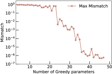
We initialize the training set for the PN surrogate with just the corner cases of the parameter space. For our 2D model, these consist of the four points: and . We augment the training set in an iterative greedy manner: At each iteration, we build a PN surrogate with the current training set, following the same methods as we use for the hybrid surrogate (see Sec. II.4). Then, we test this surrogate against a larger ( times) validation set, generated by randomly sampling the parameter space at each iteration.333 The boundary parameters are expected to be more important than those in the bulk; therefore, for 30% of the points in the validation set, we sample only from the boundary, which corresponds to the edges of a square in the 2D case. We select the parameter in the validation set that has the largest error (computed using Eq. (4)) and add it to the training set for the next iteration. We repeat this procedure until the largest validation error falls below a certain threshold.
In order to estimate the error between two complex waveforms and , we use the time-domain inner product,
| (3) |
to compute the mismatch,
| (4) |
When computing mismatches for the PN surrogate, we assume a flat noise curve, and do not optimize over time and phase shifts.
Figure 1 shows the maximum validation error at each iteration against the size of the training set. We stop this procedure when the training set size reaches 47, as the mismatch settles below at this point. Among these, 31 cases lie in the region , while 16 lie in the region . Rather than perform new NR simulations for the cases, we generate waveforms using the existing NRHybSur3dq8 model Varma et al. (2019a). This model was trained on NR-EOB/PN hybrid waveforms with mass ratios and spins , and was shown to reproduce the hybrid waveforms without a significant loss of accuracy Varma et al. (2019a).
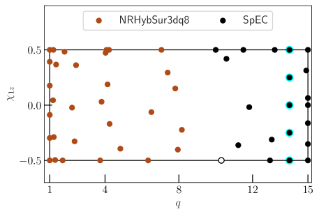
For the cases with , we perform new NR simulations using SpEC SpE ; Boyle et al. (2019). These NR waveforms include of evolution before the merger and are hybridized using SEOBNRv4HM Cotesta et al. (2018) waveforms to include the early inspiral (see Sec. II.1.2). However, of the 16 cases with , only 15 simulations were successfully completed.444The reason for failure is large constraint violation as the binary approaches merger. We believe a better domain decomposition may be needed for this simulation, which we plan to explore in the future. This leaves us with a total of 46 training waveforms (15 NR-EOB hybrid waveforms and 31 NRHybSur3dq8 waveforms).
From an initial attempt to build a hybrid surrogate with these 46 waveforms, we found that the model performs poorly for low masses , with mismatches reaching , but performs very well for higher masses, with mismatches . In other words, the late inspiral and merger-ringdown stages were accurately captured, but the early inspiral was not. This suggested that more hybrid waveforms were required. To estimate where in parameter space to place new hybrid waveforms, we first constructed a trial NR-only surrogate using the above training set of 46 waveforms, but restricted to the last before merger; we will refer to this model as NRSur2dq15. Next, we hybridized waveforms (see Sec. II.1.2) obtained from NRSur2dq15 to generate new training points in the region. This bootstrap method allowed us to create as many hybrid waveforms as necessary in the region without performing new NR simulations. After some trial and error, we found that placing five new hybrid waveforms at (uniformly distributed in ) resolved the problem at low masses.
With this insight, we finally performed five new SpEC NR simulations at these points and added the hybrid waveforms based on these to our training set for the final model, which now includes 20 NR-EOB hybrid waveforms and 31 NRHybSur3dq8 waveforms, for a total of 51 waveforms. Figure 2 shows the distribution of these parameters, including the failed simulation and the new simulations.
The new NR simulations are performed using SpEC SpE ; Boyle et al. (2019); they have been assigned identifiers SXS:BBH:2463-SXS:BBH:2482, and made publicly available through the SXS catalog SXS Collaboration . The constraint equations are solved employing the extended conformal thin sandwich formalism York (1999); Pfeiffer and York (2003) with superposed harmonic Kerr free data Varma et al. (2018). The evolution equations are solved employing the generalized harmonic formulation Lindblom et al. (2006); Rinne et al. (2009). The start time of these simulations is approximately before the peak of the waveform amplitude (defined in Eq. (5)), where is the total Christodoulou mass measured after the initial burst of junk radiation Boyle et al. (2019). The initial orbital parameters are chosen through an iterative procedure Buonanno et al. (2011) such that the orbits are quasicircular; the largest eccentricity for these simulations is , while the median value is . The waveforms are extracted at several extraction surfaces at varying finite radii form the origin and then extrapolated to future null infinity Boyle and Mroue (2009). Finally, the extrapolated waveforms are corrected to account for the initial drift of the center of mass Woodford et al. (2019).
II.1.2 Hybridization
Given the new NR waveforms, we now hybridize them by smoothly attaching an EOB waveform for the early inspiral. For the previous NR hybrid surrogate model NRHybSur3dq8 Varma et al. (2019a), a combination of PN and EOB was used for the early inspiral: the amplitudes for all modes were obtained from PN, while the phase evolution for all modes was derived from the (2,2) mode of the SEOBNRv4 EOB model Bohé et al. (2017) (see Sec. IV.B of Ref. Varma et al. (2019a)). This was motivated by the fact that the PN mode amplitudes were found to be accurate enough for hybridizing NR simulations, while the PN mode phases were not (see Fig. 3 of Ref. Varma et al. (2019a)).
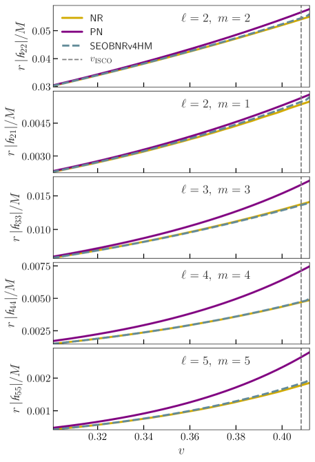
We find that the same strategy does not work for the large cases considered in this work. Figure 3 shows a comparison between the mode amplitudes of NR, PN and the SEOBNRv4HM EOB model Cotesta et al. (2018), for a system. We show all modes [(2,2), (2,1), (3,3), (4,4), and (5,5)] included by SEOBNRv4HM, which is an extension of the SEOBNRv4 model. The PN waveforms are described in Sec. II.1.1; we include amplitudes terms up to 3.5 PN order Blanchet et al. (2008); Faye et al. (2012, 2015). In Fig. 3, the PN amplitudes (especially for the subdominant modes) deviate significantly from NR , while SEOBNRv4HM shows excellent agreement. This is not surprising, as SEOBNRv4HM is calibrated to NR waveforms, as well as some BH perturbation theory waveforms at extreme mass ratios Cotesta et al. (2018). We conclude that current PN waveforms are not suitable for hybridizing NR waveforms at large mass ratios like . Therefore, in this work, we only use SEOBNRv4HM for hybridizing NR waveforms. Unfortunately, this means that our new model NRHybSur2dq15 is restricted to the same set of modes as SEOBNRv4HM.
We follow the same hybridization procedure as Sec. V of Ref. Varma et al. (2019a) to smoothly attach SEOBNRv4HM inspirals to the 20 new NR simulations obtained in Sec. II.1.1. For the remaining 31 training cases with , we generate waveforms using the NRHybSur3dq8 model, as it is already hybridized. This completes the construction of our training set waveforms.
II.2 Frame alignment
We follow Ref. Varma et al. (2019a) and apply the following post processing to the training set waveforms. This ensures that all waveforms are in the same frame, and therefore that the data used in the surrogate fits (see Sec. II.4) vary smoothly across parameter space.
II.2.1 Time alignment
We apply a time shift to each training waveform such that peak of the total amplitude
| (5) |
occurs at . The original peak time is determined by a quadratic fit using 5 time samples adjacent to the discrete maximum of Blackman et al. (2017a).
II.2.2 Down-sampling and common time array
The length of each hybrid waveform is set by choosing a starting orbital frequency for the SEOBNRv4HM inspiral; we use for all waveforms. However, for the same starting frequency, the waveform length in time is different for different mass ratios and spins. On the other hand, the surrogate modeling procedure requires that all training waveforms have a common time array Field et al. (2014). Therefore, we truncate all waveforms such that they start at the same initial time ( before the peak), which is determined by the shortest hybrid waveform in the training set. Post truncation, the largest starting orbital frequency is , which sets the low-frequency limit of validity of the surrogate. For LIGO and Virgo, assuming a starting GW frequency of , the mode of the surrogate model is valid for total masses . The highest spin-weighted spherical harmonic mode included in the model is , for which the corresponding frequency is 5/2 times that of the mode. Therefore, all modes of the surrogate are valid for .
Because the hybrid waveforms are very long, it is not practical to sample the entire waveform with a small uniform time step like , as is typically done for NR-only surrogates Varma et al. (2019b). Fortunately, the early low-frequency portion of the waveform does not require as dense a time sampling as the later high-frequency portion. We therefore down-sample the time arrays of the truncated hybrid waveforms to a common set of time samples. We choose the time samples such that there are points per orbit for the above-mentioned shortest hybrid waveform in the training set. However, for we switch to uniformly spaced time samples with a time step of . This ensures that we have a sufficiently dense sampling rate for the late inspiral and the merger-ringdown where the frequency reaches its peak. We retain times up to after the peak, which is sufficient to capture the entire ringdown.
Given the common down-sampled time array, we use cubic splines to interpolate all waveforms in the training set to these times. However, we first transform the waveforms into the co-orbital frame, defined as:
| (6) | |||
| (7) | |||
| (8) |
where is the inertial frame waveform, is the orbital phase, and and are the amplitude and phase of the mode. The co-orbital frame can be seen as roughly co-rotating with the binary, obtained by applying a time-dependent rotation about the axis, by an amount given by the instantaneous orbital phase. Therefore, the waveform is a slowly varying function of time in this frame, which increases the interpolation accuracy. For the (2, 2) mode we save the downsampled amplitude and phase , while for all other modes we save the real and imaginary parts of .
II.2.3 Phase alignment
Finally, we rotate the waveforms about the -axis such that the orbital phase is zero at . Note that this by itself would fix the physical rotation up to a shift of . When generating the EOB inspiral waveform for hybridization, the frame is aligned such that heavier BH is on the positive -axis at the initial time, which fixes the ambiguity Varma et al. (2019a). After the phase alignment, the heavier BH is on the positive -axis at for all waveforms. However, keep in mind that this frame is defined using the waveform at future null infinity, and these BH positions do not necessarily correspond to the (gauge-dependent) coordinate BH positions in the NR simulations.
II.3 Data decomposition
It is much easier to build a model for slowly varying functions of time. Therefore, we decompose the inertial frame strain , which is oscillatory, into simpler “waveform data pieces” and build a separate surrogate for each data piece. When evaluating the full surrogate model, we first evaluate the surrogate for each data piece and then combine the data pieces to get the inertial frame strain. The mode is decomposed into its amplitude and phase (which is further decomposed below). For the other modes, we model the real and imaginary parts of the co-orbital frame strain (see Eq. (6)).
Following Ref. Varma et al. (2019b), we further decompose by subtracting the leading-order prediction from the TaylorT3 PN approximant Damour et al. (2001), given by:
| (9) |
where is an arbitrary integration constant, , is an arbitrary time offset, and is the symmetric mass ratio. Because diverges at , we choose , long after the peak () of the waveform, ensuring that we are always far away from this divergence. We choose such that at , which is the same time at which we align the hybrid phase in Sec. II.2.3.
By modeling the difference instead of , we automatically capture almost all of the phase evolution in the early inspiral of the long hybrid waveforms. Therefore, we simplify the problem of modeling the phase to the same as modeling the phase of NR-only waveforms. This improves the overall accuracy of the surrogate model for low masses, for which the inspiral dominates. We stress that the exact form of (or its physical meaning) is not important because we add the exact same to our model of when evaluating the surrogate. In fact, even though TaylorT3 is known to be less accurate than other approximants Buonanno et al. (2009); Varma et al. (2013), its speed (being a simple, analytic, closed-form, function of time) makes it ideal for our purpose.
To summarize, we decompose the hybrid waveforms into the following waveform data pieces, each of which is a smooth, slowly varying function of time: for the mode, and the real and imaginary parts of for the (2,1), (3,3), (4,4) and (5,5) modes.
II.4 Surrogate construction and evaluation
Given the waveform data pieces, we build a surrogate model for each data piece using the same procedure as Sec.V.C of Ref. Varma et al. (2019a), which we summarize below.
For each waveform data piece, we first construct a linear basis using the greedy basis method Field et al. (2011), with tolerances of radians for the data piece and for all other data pieces. Next, we construct an empirical time interpolant Barrault et al. (2004); Maday et al. (2009); Hesthaven, Jan S. et al. (2014) with the same number of empirical time nodes as basis functions for that data piece. Finally, for each empirical time node, we construct a parametric fit for the waveform data piece, following the Gaussian process regression (GPR) fitting method, as described in Refs. Varma et al. (2019c); Taylor and Varma (2020). The fits are parameterized by , where
| (10) |
is the spin parameter entering the GW phase at leading order Ajith (2011), and is the effective spin. Note that in the above expressions for the current surrogate, but we adopt this parameterization to be consistent with Ref. Varma et al. (2019a). In practice, parameterizing the fits by also leads to a surrogate of similar accuracy. On the other hand, the parameterization leads to a significant improvement in model accuracy, in agreement with Refs. Varma et al. (2019a); Rifat et al. (2020).
When evaluating the surrogate waveform, we first evaluate each surrogate waveform data piece. Next, we compute the mode phase:
| (11) |
where is the surrogate model for , and is given by Eq. (9). If the waveform is required at a uniform sampling rate, we interpolate each waveform data piece from the sparse time samples to the required time samples using a cubic-spline interpolation scheme. Finally, we use Eqs. (6), (7), and (8) to reconstruct the inertial frame strain.
III Surrogate errors
In this section, we evaluate the accuracy of NRHybSur2dq15 by comparing against NR-EOB hybrid waveforms. Similarly, we compute errors for two semi-analytic waveform models, the phenomenological model IMRPhenomTHM Estellés et al. (2020) and the EOB model SEOBNRv4HM Cotesta et al. (2018). Both of these models are calibrated against nonprecessing NR simulations and include the same set of modes as NRHybSur2dq15 and the hybrid waveforms: (2,2), (2,1), (3,3), (4,4) and (5,5). Other semi-analytic nonprecessing models that include subdominant modes exist in literature, including Refs Nagar et al. (2020); García-Quirós et al. (2020), but we do not consider these models for simplicity (as they have accuracies comparable Nagar et al. (2020); García-Quirós et al. (2020); Nagar et al. (2022) to IMRPhenomTHM and SEOBNRv4HM).
In order to estimate the difference between two waveforms, and , we compute the mismatch (Eq. 4) using the noise-weighted inner product in frequency-domain, defined as
| (12) |
where indicates the Fourier transform of the complex strain , ∗ indicates a complex conjugation, indicates the real part, and is the one-sided power spectral density of a GW detector. We use the Advanced-LIGO design sensitivity Zero-Detuned-HighP noise curve LIGO Scientific Collaboration (2018), with Hz and Hz. We compute the mismatches following the procedure described in Sec.VII of Ref. Varma et al. (2019a): the mismatches are optimized over shifts in time, polarization angle, and initial orbital phase. Both plus and cross polarizations are treated on an equal footing by using a two-detector setup where one detector sees only the plus and the other only the cross polarization. We use all the available modes of a given waveform model, and compute the mismatches at 37 points uniformly distributed on the sky in the source frame.
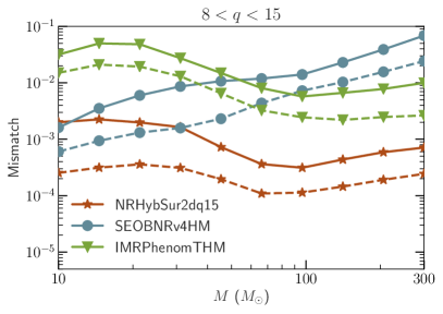
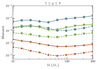
Figure 4 shows mismatches computed using the Advanced-LIGO noise curve for NRHybSur2dq15, SEOBNRv4HM and IMRPhenomTHM against hybrid waveforms. As these depend on the total mass, we show mismatches for various masses, starting near the lower limit of the range of validity of the surrogate . At each mass, we show the median and 95th percentile mismatches, over many hybrid waveforms and points in the source frame sky.
The left panel of Fig. 4 shows mismatches against the 20 NR-EOB hybrid waveforms in Fig. 2. As these hybrid waveforms were also used in the training of NRHybSur2dq15, we conduct a leave-one-out analysis: we generate 20 trial surrogates, leaving out one of the hybrid waveforms from the training set in each trial, but including the rest of the training cases (both and ) in Fig. 2. For each trial surrogate, we compute errors against the hybrid waveform that was left out. In this manner, we only compare NRHybSur2dq15 against waveforms not used in the model training. Therefore, these errors are indicative of the true modeling error.
For the region, 95th percentile mismatches for NRHybSur2dq15 fall below over the entire mass range in Fig. 4. The errors for IMRPhenomTHM and SEOBNRv4HM are generally larger by at least an order of magnitude. However, for SEOBNRv4HM, the errors at low masses overlap with the surrogate errors. This is most likely because SEOBNRv4HM was used to generate the early inspiral waveform for the NR-EOB hybrid waveforms. At low masses, where the early inspiral dominates the overall error budget, these errors are therefore not representative of the true error in SEOBNRv4HM.
The right panel of Fig. 4 shows mismatches in the region. In this region, rather than conduct leave-one-out tests, we simply generate 100 new hybrid waveforms using the NRHybSur3dq8 model for testing. These test cases are uniformly distributed in the region and , with . Once again NRHybSur2dq15 has mismatches that are at least an order of magnitude smaller than that of SEOBNRv4HM and IMRPhenomTHM. In this case, SEOBNRv4HM errors are broadly uniform across all masses. This is most likely explained by the fact that the early inspiral of NRHybSur3dq8 was based on PN as well as EOB waveforms; more precisely, PN was directly used to generate the mode amplitudes while the (2,2) mode of SEOBNRv4HM (the SEOBNRv4 Bohé et al. (2017) model) was used to correct the PN mode phases.
While Fig. 4 shows model errors when including all available modes, it can be useful to also understand the errors in the individual modes. We quantify this using the normalized norm between two waveforms and :
| (13) |
This error measure was introduced in Ref. Blackman et al. (2017b) and is related to weighted average of the mismatch over the sky in the source frame. When computing , we only consider the late inspiral and merger-ringdown region by choosing and . As the NR waveforms used in generating the hybrid waveforms had typical start times (see Sec. II.1), this ensures that is independent of which model was used in the hybridization procedure. Furthermore, rather than optimizing over time or phase shifts, we simply align the frames of the two waveforms such that the peak amplitude (Eq. (5)) occurs at , and the orbital phase (Eq. (8)) is zero at . This makes much cheaper to evaluate than the mismatches in Eq. (12). In addition to computing normalized errors using all available modes, we also consider single-mode errors by restricting the sums in Eq. (13) to individual modes.
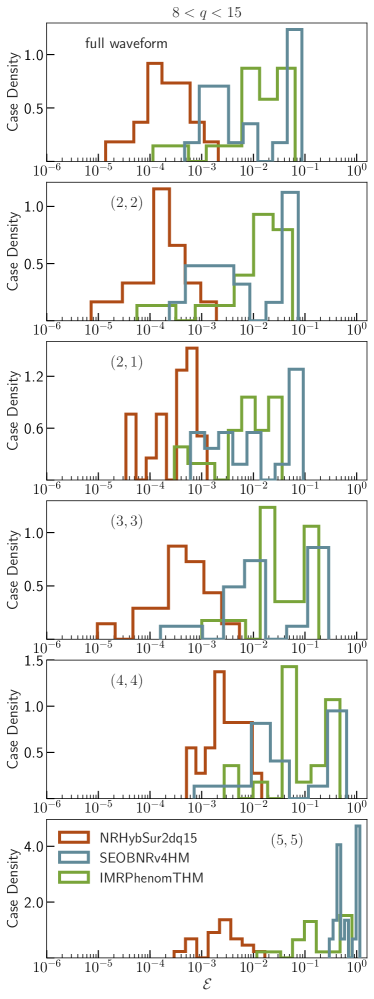
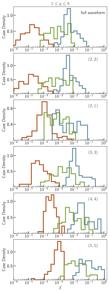
Figure 5 shows normalized errors for NRHybSur2dq15, SEOBNRv4HM and IMRPhenomTHM against hybrid waveforms. The left panel of Fig. 5 follows the left panel of Fig. 4, and shows errors for the three waveform models (using a leave-one-out analysis for NRHybSur2dq15) against the 20 NR-EOB hybrid waveforms. The right panel of Fig. 5 follows the right panel of Fig. 4, and shows errors against the same 100 uniformly distributed NRHybSur3dq8 waveforms in the region and , with . For both and , we once again find that NRHybSur2dq15 is more accurate than the other models by at least an order of magnitude, both for the full waveform and for the individual modes.
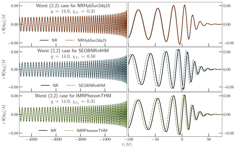
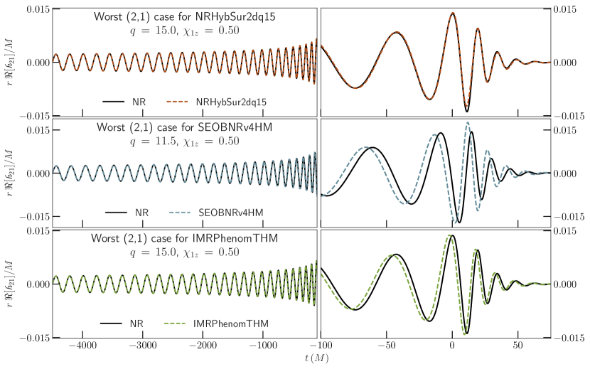
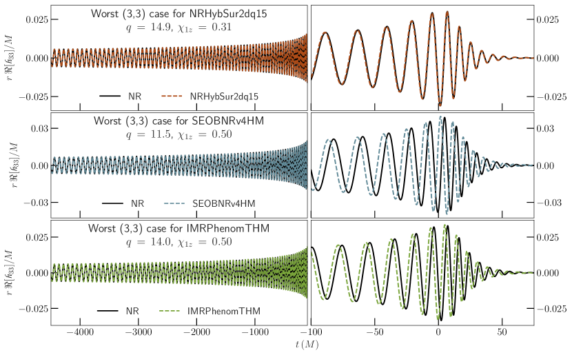
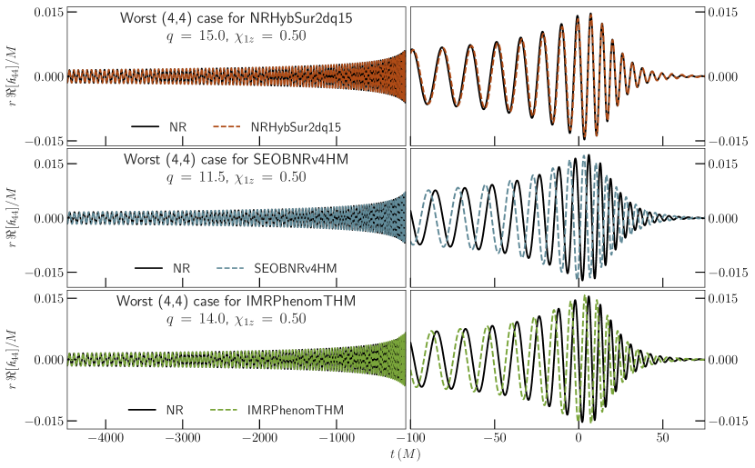
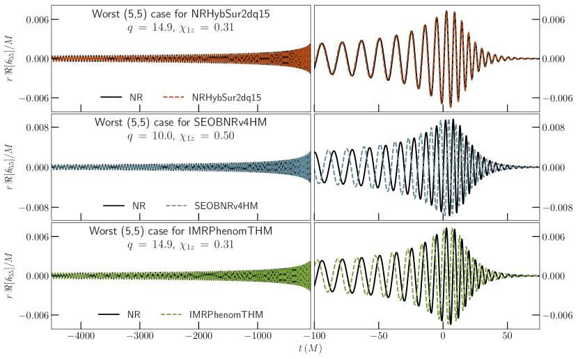
Considering the individual mode errors in Fig. 5, we note that the fractional errors in the nonquadrupole modes of SEOBNRv4HM and IMRPhenomTHM reach large values. In particular, the errors in the (5,5) mode for SEOBNRv4HM for can reach values . While the nonquadrupole modes are still subdominant for binaries like GW190814 (which is why the full waveform errors do not reach such large values in Fig. 5), it may be important for models like IMRPhenomTHM and SEOBNRv4HM to improve accuracy in these modes for future observations. Finally, to illustrate the (in)accuracy of the individual modes, Figs. 6, 7 and 8 show the cases leading to the largest individual mode errors in the left panel of Fig. 5.
III.1 Extrapolating outside the training region
The errors computed so far were restricted to the training region of NRHybSur2dq15: , , and . It is possible to extrapolate the model to larger and , but it is difficult to assess the model accuracy in this region due to a lack of NR simulations. Instead, through a visual inspection of the evaluated waveforms, we find that extrapolating beyond or leads to unphysical “glitches” in the time series for the mode amplitudes and the derivatives of the mode phases. Therefore, while we allow the model to be evaluated in the region , , and , we advise caution when extrapolating the model.
IV Reanalyzing GW190814
NRHybSur2dq15 is targeted towards GW events like GW190814 Abbott et al. (2020), with mass ratios . As NRHybSur2dq15 is more accurate than alternative models in this region, we now reanalyze GW190814 with NRHybSur2dq15. In addition, we consider two phenomenological models, IMRPhenomTHM Estellés et al. (2020) and IMRPhenomTPHM Estellés et al. (2021). Both of these models include the effects of subdominant modes, but only IMRPhenomTPHM includes precession effects. Precession effects are included in IMRPhenomTPHM by “twisting” the frame of the nonprecessing model IMRPhenomTHM to mimic orbital precession Estellés et al. (2021). The GW190814 discovery paper Abbott et al. (2020) instead considered the SEOBNRv4PHM Ossokine et al. (2020) and IMRPhenomPv3PHM Khan et al. (2020) binary BH models, both of which include the effects of subdominant modes and precession (through a similar twisting procedure). For simplicity, we do not consider these models here, but we have verified that our results with IMRPhenomTPHM are consistent with Ref. Abbott et al. (2020). Ref. Abbott et al. (2020) also considered models Matas et al. (2020); Thompson et al. (2020) with tidal effects, but found no measurable tidal signatures; therefore, we only show results for binary BH models.
Source properties can be inferred from GW data following Bayes’ theorem (see e.g. Ref. Thrane and Talbot (2019) for a review). We analyze the GW190814 data made public by the LIGO-Virgo-Kagra Collaboration Abbott et al. (2020); Collaboration and Collaboration , using the Parallel Bilby Smith et al. (2020) parameter estimation package with the dynesty Speagle (2020) sampler. Following Ref. Abbott et al. (2021b), we choose a prior that is uniform in detector frame component masses, and isotropic in sky location and binary orientation. For the distance prior, we use the UniformSourceFrame prior Romero-Shaw et al. (2020) assuming a cosmology from Ade et al. (2016) as implemented in Astropy Robitaille et al. (2013); Price-Whelan et al. (2018).
When using the nonprecessing models NRHybSur2dq15 and IMRPhenomTHM, we use the AlignedSpin prior Romero-Shaw et al. (2020); Callister (2021), with and . The AlignedSpin prior follows the generic-spin assumptions of a prior that is uniform in magnitude and isotropic in orientation for each of the two spin vectors, which in the nonprecessing case is projected onto the orbital angular momentum. Even though IMRPhenomTHM allows generic aligned-spins on both BHs, we restrict the model to the same spin range as NRHybSur2dq15 for easy comparison. We have, however, verified that using unrestricted aligned-spins for IMRPhenomTHM has a negligible impact on GW190814 posteriors; this is expected as Ref. Abbott et al. (2020) placed a constraint of at 90% credibility, and found that cannot be constrained for GW190814. When using the precessing model IMRPhenomTPHM, our prior is uniform in spin magnitudes (with ) and isotropic in spin orientations for both BHs. The reason for considering a precessing model with no spin restrictions is to gauge the impact of neglecting precession in NRHybSur2dq15.
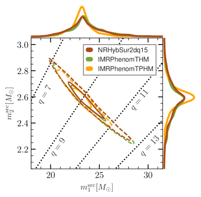
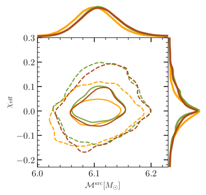
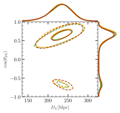
Figure 9 shows posterior distributions for the GW190814 source parameters obtained using NRHybSur2dq15, IMRPhenomTHM and IMRPhenomTPHM. We show constraints on the source-frame component masses and , the effective spin , the source-frame chirp mass , the luminosity distance , and cosine of the inclination angle between the total angular momentum and the line of sight direction . As NRHybSur2dq15 is significantly more accurate (see Fig. 4), the differences between NRHybSur2dq15 and IMRPhenomTHM can be used to gauge systematic uncertainties in IMRPhenomTHM. In Fig. 9 we find good agreement between NRHybSur2dq15 and IMRPhenomTHM for all parameters shown, which suggests that semi-analytical models like IMRPhenomTHM are accurate enough for events like GW190814. However, this may not be the case as detector sensitivity improves and GW190814-like signals are observed at larger SNRs. At larger SNRs, the differences noted in Figs. 4 and 5 can become significant.
Finally, comparing the posteriors for IMRPhenomTHM and IMRPhenomTPHM in Fig. 9, we find that including the effects of precession leads to stronger constraints on the component masses and , while the chirp mass, distance and inclination constraints are not significantly affected. This is in agreement with Ref. Abbott et al. (2020), and implies that precession effects should be included in NRHybSur2dq15. While this can be done by a frame twisting procedure similar to IMRPhenomTPHM, this method does not capture the full effects of precession like the asymmetries between pairs of and spin-weighted spherical harmonic modes Varma et al. (2019b, 2021). While precessing NR surrogate models Varma et al. (2019b) capture these effects, they require NR simulations, which are not currently possible at large mass ratios. Therefore, we leave this exploration to future work.
V Conclusion
We present NRHybSur2dq15, a surrogate waveform model targeted at large mass ratio GW events like GW190814. The model is trained on 51 binary BH hybrid waveforms with mass ratios and aligned spins , , includes the (2,2), (2,1), (3,3), (4,4), and (5,5) spin-weighted spherical harmonic modes, and spans the entire LIGO-Virgo bandwidth (with Hz) for total masses . Through a leave-one-out study, we show that NRHybSur2dq15 accurately reproduces the hybrid waveforms, with mismatches below for total masses . This is at least an order-of-magnitude improvement over existing semi-analytical models. The model is made publicly available through the easy-to-use Python package gwsurrogate Blackman et al. .
We reanalyze GW190814 using NRHybSur2dq15 and find results consistent with the discovery paper Ref. Abbott et al. (2020). This suggests that current semi-analytical models are accurate enough for events like GW190814. However, as detector sensitivity improves, we can expect to see similar signals at a higher SNR. We anticipate that accurate models like NRHybSur2dq15 will be necessary for analyzing such signals. With that goal, we identify precession as an important feature to be added to NRHybSur2dq15 in the future.
Acknowledgements.
We thank Hector Estelles and Alessandro Nagar for comments on the manuscript. This work was supported in part by the Sherman Fairchild Foundation and by National Science Foundation (NSF) Grant Nos. PHY-2011961, PHY-2011968, and OAC-1931266 at Caltech, and NSF Grant Nos. PHY-1912081 and OAC-1931280 at Cornell. V.V. acknowledges funding from the European Union’s Horizon 2020 research and innovation program under the Marie Skłodowska-Curie grant agreement No. 896869. V.V. was supported by a Klarman Fellowship at Cornell. C.-J.H. acknowledges support of the NSF and the LIGO Laboratory. NR simulations were conducted on the Frontera computing project at the Texas Advanced Computing Center. Additional computations were performed on the Wheeler cluster at Caltech, which is supported by the Sherman Fairchild Foundation and by Caltech; and the High Performance Cluster at Caltech. This material is based upon work supported by NSF’s LIGO Laboratory which is a major facility fully funded by the NSF. This research made use of data, software and/or web tools obtained from the Gravitational Wave Open Science Center Collaboration and Collaboration , a service of the LIGO Laboratory, the LIGO Scientific Collaboration and the Virgo Collaboration.References
- Aasi et al. (2015) J. Aasi et al. (LIGO Scientific), “Advanced LIGO,” Class. Quant. Grav. 32, 074001 (2015), arXiv:1411.4547 [gr-qc] .
- Acernese et al. (2015) F. Acernese et al. (Virgo), “Advanced Virgo: a second-generation interferometric gravitational wave detector,” Class. Quant. Grav. 32, 024001 (2015), arXiv:1408.3978 [gr-qc] .
- Abbott et al. (2019) B. P. Abbott et al. (LIGO Scientific, Virgo), “GWTC-1: A Gravitational-Wave Transient Catalog of Compact Binary Mergers Observed by LIGO and Virgo during the First and Second Observing Runs,” Phys. Rev. X9, 031040 (2019), arXiv:1811.12907 [astro-ph.HE] .
- Abbott et al. (2021a) R. Abbott et al. (LIGO Scientific, VIRGO), “GWTC-2.1: Deep Extended Catalog of Compact Binary Coalescences Observed by LIGO and Virgo During the First Half of the Third Observing Run,” (2021a), arXiv:2108.01045 [gr-qc] .
- Abbott et al. (2021b) R. Abbott et al. (LIGO Scientific, VIRGO, KAGRA), “GWTC-3: Compact Binary Coalescences Observed by LIGO and Virgo During the Second Part of the Third Observing Run,” (2021b), arXiv:2111.03606 [gr-qc] .
- Abbott et al. (2016) B. P. Abbott et al. (LIGO Scientific, Virgo), “Observation of Gravitational Waves from a Binary Black Hole Merger,” Phys. Rev. Lett. 116, 061102 (2016), arXiv:1602.03837 [gr-qc] .
- Abbott et al. (2017) Benjamin P. Abbott et al. (LIGO Scientific, Virgo), “GW170817: Observation of Gravitational Waves from a Binary Neutron Star Inspiral,” Phys. Rev. Lett. 119, 161101 (2017), arXiv:1710.05832 [gr-qc] .
- Abbott et al. (2021c) R. Abbott et al. (LIGO Scientific, KAGRA, VIRGO), “Observation of Gravitational Waves from Two Neutron Star–Black Hole Coalescences,” Astrophys. J. Lett. 915, L5 (2021c), arXiv:2106.15163 [astro-ph.HE] .
- Abbott et al. (2020) R. Abbott et al. (LIGO Scientific, Virgo), “GW190814: Gravitational Waves from the Coalescence of a 23 Solar Mass Black Hole with a 2.6 Solar Mass Compact Object,” Astrophys. J. Lett. 896, L44 (2020), arXiv:2006.12611 [astro-ph.HE] .
- Godzieba et al. (2021) Daniel A. Godzieba, David Radice, and Sebastiano Bernuzzi, “On the maximum mass of neutron stars and GW190814,” Astrophys. J. 908, 122 (2021), arXiv:2007.10999 [astro-ph.HE] .
- Dexheimer et al. (2021) V. Dexheimer, R. O. Gomes, T. Klähn, S. Han, and M. Salinas, “GW190814 as a massive rapidly rotating neutron star with exotic degrees of freedom,” Phys. Rev. C 103, 025808 (2021), arXiv:2007.08493 [astro-ph.HE] .
- Clesse and Garcia-Bellido (2020) Sebastien Clesse and Juan Garcia-Bellido, “GW190425, GW190521 and GW190814: Three candidate mergers of primordial black holes from the QCD epoch,” (2020), arXiv:2007.06481 [astro-ph.CO] .
- Tews et al. (2021) Ingo Tews, Peter T. H. Pang, Tim Dietrich, Michael W. Coughlin, Sarah Antier, Mattia Bulla, Jack Heinzel, and Lina Issa, “On the Nature of GW190814 and Its Impact on the Understanding of Supranuclear Matter,” Astrophys. J. Lett. 908, L1 (2021), arXiv:2007.06057 [astro-ph.HE] .
- Tsokaros et al. (2020) Antonios Tsokaros, Milton Ruiz, and Stuart L. Shapiro, “GW190814: Spin and equation of state of a neutron star companion,” Astrophys. J. 905, 48 (2020), arXiv:2007.05526 [astro-ph.HE] .
- Fattoyev et al. (2020) F. J. Fattoyev, C. J. Horowitz, J. Piekarewicz, and Brendan Reed, “GW190814: Impact of a 2.6 solar mass neutron star on the nucleonic equations of state,” Phys. Rev. C 102, 065805 (2020), arXiv:2007.03799 [nucl-th] .
- Zhang and Li (2020) Nai-Bo Zhang and Bao-An Li, “GW190814’s Secondary Component with Mass 2.50–2.67 M ⊙ as a Superfast Pulsar,” Astrophys. J. 902, 38 (2020), arXiv:2007.02513 [astro-ph.HE] .
- Tan et al. (2020) Hung Tan, Jacquelyn Noronha-Hostler, and Nico Yunes, “Neutron Star Equation of State in light of GW190814,” Phys. Rev. Lett. 125, 261104 (2020), arXiv:2006.16296 [astro-ph.HE] .
- Nathanail et al. (2021) Antonios Nathanail, Elias R. Most, and Luciano Rezzolla, “GW170817 and GW190814: tension on the maximum mass,” Astrophys. J. Lett. 908, L28 (2021), arXiv:2101.01735 [astro-ph.HE] .
- Pretorius (2005) Frans Pretorius, “Evolution of binary black hole spacetimes,” Phys. Rev. Lett. 95, 121101 (2005), arXiv:gr-qc/0507014 [gr-qc] .
- Campanelli et al. (2006) Manuela Campanelli, C. O. Lousto, P. Marronetti, and Y. Zlochower, “Accurate evolutions of orbiting black-hole binaries without excision,” Phys. Rev. Lett. 96, 111101 (2006), arXiv:gr-qc/0511048 [gr-qc] .
- Baker et al. (2006) John G. Baker, Joan Centrella, Dae-Il Choi, Michael Koppitz, and James van Meter, “Gravitational wave extraction from an inspiraling configuration of merging black holes,” Phys. Rev. Lett. 96, 111102 (2006), arXiv:gr-qc/0511103 [gr-qc] .
- Boyle et al. (2019) Michael Boyle et al., “The SXS Collaboration catalog of binary black hole simulations,” Class. Quant. Grav. 36, 195006 (2019), arXiv:1904.04831 [gr-qc] .
- Ossokine et al. (2020) Serguei Ossokine et al., “Multipolar Effective-One-Body Waveforms for Precessing Binary Black Holes: Construction and Validation,” Phys. Rev. D 102, 044055 (2020), arXiv:2004.09442 [gr-qc] .
- Khan et al. (2020) Sebastian Khan, Frank Ohme, Katerina Chatziioannou, and Mark Hannam, “Including higher order multipoles in gravitational-wave models for precessing binary black holes,” Phys. Rev. D 101, 024056 (2020), arXiv:1911.06050 [gr-qc] .
- Matas et al. (2020) Andrew Matas et al., “Aligned-spin neutron-star–black-hole waveform model based on the effective-one-body approach and numerical-relativity simulations,” Phys. Rev. D 102, 043023 (2020), arXiv:2004.10001 [gr-qc] .
- Thompson et al. (2020) Jonathan E. Thompson, Edward Fauchon-Jones, Sebastian Khan, Elisa Nitoglia, Francesco Pannarale, Tim Dietrich, and Mark Hannam, “Modeling the gravitational wave signature of neutron star black hole coalescences,” Phys. Rev. D 101, 124059 (2020), arXiv:2002.08383 [gr-qc] .
- Cotesta et al. (2018) Roberto Cotesta, Alessandra Buonanno, Alejandro Bohé, Andrea Taracchini, Ian Hinder, and Serguei Ossokine, “Enriching the Symphony of Gravitational Waves from Binary Black Holes by Tuning Higher Harmonics,” Phys. Rev. D98, 084028 (2018), arXiv:1803.10701 [gr-qc] .
- Estellés et al. (2021) Héctor Estellés, Marta Colleoni, Cecilio García-Quirós, Sascha Husa, David Keitel, Maite Mateu-Lucena, Maria de Lluc Planas, and Antoni Ramos-Buades, “New twists in compact binary waveform modelling: a fast time domain model for precession,” (2021), arXiv:2105.05872 [gr-qc] .
- Estellés et al. (2020) Héctor Estellés, Sascha Husa, Marta Colleoni, David Keitel, Maite Mateu-Lucena, Cecilio García-Quirós, Antoni Ramos-Buades, and Angela Borchers, “Time domain phenomenological model of gravitational wave subdominant harmonics for quasi-circular non-precessing binary black hole coalescences,” (2020), arXiv:2012.11923 [gr-qc] .
- Pratten et al. (2021) Geraint Pratten et al., “Computationally efficient models for the dominant and subdominant harmonic modes of precessing binary black holes,” Phys. Rev. D 103, 104056 (2021), arXiv:2004.06503 [gr-qc] .
- García-Quirós et al. (2020) Cecilio García-Quirós, Marta Colleoni, Sascha Husa, Héctor Estellés, Geraint Pratten, Antoni Ramos-Buades, Maite Mateu-Lucena, and Rafel Jaume, “Multimode frequency-domain model for the gravitational wave signal from nonprecessing black-hole binaries,” Phys. Rev. D 102, 064002 (2020), arXiv:2001.10914 [gr-qc] .
- Akcay et al. (2021) Sarp Akcay, Rossella Gamba, and Sebastiano Bernuzzi, “Hybrid post-Newtonian effective-one-body scheme for spin-precessing compact-binary waveforms up to merger,” Phys. Rev. D 103, 024014 (2021), arXiv:2005.05338 [gr-qc] .
- Nagar et al. (2020) Alessandro Nagar, Gunnar Riemenschneider, Geraint Pratten, Piero Rettegno, and Francesco Messina, “Multipolar effective one body waveform model for spin-aligned black hole binaries,” Phys. Rev. D 102, 024077 (2020), arXiv:2001.09082 [gr-qc] .
- Varma et al. (2021) Vijay Varma, Maximiliano Isi, Sylvia Biscoveanu, Will M. Farr, and Salvatore Vitale, “Measuring binary black hole orbital-plane spin orientations,” (2021), arXiv:2107.09692 [astro-ph.HE] .
- Varma et al. (2019a) Vijay Varma, Scott E. Field, Mark A. Scheel, Jonathan Blackman, Lawrence E. Kidder, and Harald P. Pfeiffer, “Surrogate model of hybridized numerical relativity binary black hole waveforms,” Phys. Rev. D99, 064045 (2019a), arXiv:1812.07865 [gr-qc] .
- Varma et al. (2019b) Vijay Varma, Scott E. Field, Mark A. Scheel, Jonathan Blackman, Davide Gerosa, Leo C. Stein, Lawrence E. Kidder, and Harald P. Pfeiffer, “Surrogate models for precessing binary black hole simulations with unequal masses,” Phys. Rev. Research. 1, 033015 (2019b), arXiv:1905.09300 [gr-qc] .
- Field et al. (2014) S. E. Field, C. R. Galley, J. S. Hesthaven, J. Kaye, and M. Tiglio, “Fast Prediction and Evaluation of Gravitational Waveforms Using Surrogate Models,” Phys. Rev. X 4, 031006 (2014), arXiv:1308.3565 [gr-qc] .
- Blackman et al. (2017a) Jonathan Blackman, Scott E. Field, Mark A. Scheel, Chad R. Galley, Christian D. Ott, Michael Boyle, Lawrence E. Kidder, Harald P. Pfeiffer, and Béla Szilágyi, “Numerical relativity waveform surrogate model for generically precessing binary black hole mergers,” Phys. Rev. D96, 024058 (2017a), arXiv:1705.07089 [gr-qc] .
- Lousto and Healy (2020) Carlos O. Lousto and James Healy, “Exploring the Small Mass Ratio Binary Black Hole Merger via Zeno’s Dichotomy Approach,” Phys. Rev. Lett. 125, 191102 (2020), arXiv:2006.04818 [gr-qc] .
- Abbott et al. (2021d) R. Abbott et al. (LIGO Scientific, VIRGO, KAGRA), “The population of merging compact binaries inferred using gravitational waves through GWTC-3,” (2021d), arXiv:2111.03634 [astro-ph.HE] .
- Varma and Ajith (2017) Vijay Varma and Parameswaran Ajith, “Effects of nonquadrupole modes in the detection and parameter estimation of black hole binaries with nonprecessing spins,” Phys. Rev. D96, 124024 (2017), arXiv:1612.05608 [gr-qc] .
- Varma et al. (2014) Vijay Varma, Parameswaran Ajith, Sascha Husa, Juan Calderon Bustillo, Mark Hannam, and Michael Pürrer, “Gravitational-wave observations of binary black holes: Effect of nonquadrupole modes,” Phys. Rev. D90, 124004 (2014), arXiv:1409.2349 [gr-qc] .
- Capano et al. (2014) Collin Capano, Yi Pan, and Alessandra Buonanno, “Impact of higher harmonics in searching for gravitational waves from nonspinning binary black holes,” Phys. Rev. D89, 102003 (2014), arXiv:1311.1286 [gr-qc] .
- Shaik et al. (2020) Feroz H. Shaik, Jacob Lange, Scott E. Field, Richard O’Shaughnessy, Vijay Varma, Lawrence E. Kidder, Harald P. Pfeiffer, and Daniel Wysocki, “Impact of subdominant modes on the interpretation of gravitational-wave signals from heavy binary black hole systems,” Phys. Rev. D 101, 124054 (2020), arXiv:1911.02693 [gr-qc] .
- Islam et al. (2021) Tousif Islam, Scott E. Field, Carl-Johan Haster, and Rory Smith, “High precision source characterization of intermediate mass-ratio black hole coalescences with gravitational waves: The importance of higher order multipoles,” Phys. Rev. D 104, 084068 (2021), arXiv:2105.04422 [gr-qc] .
- (46) “The Spectral Einstein Code,” http://www.black-holes.org/SpEC.html.
- (47) “Simulating eXtreme Spacetimes,” http://www.black-holes.org/.
- Apostolatos et al. (1994) Theocharis A. Apostolatos, Curt Cutler, Gerald J. Sussman, and Kip S. Thorne, “Spin-induced orbital precession and its modulation of the gravitational waveforms from merging binaries,” Phys. Rev. D 49, 6274–6297 (1994).
- Schmidt et al. (2015) P. Schmidt, F. Ohme, and M. Hannam, “Towards models of gravitational waveforms from generic binaries II: Modelling precession effects with a single effective precession parameter,” Phys. Rev. D 91, 024043 (2015), arXiv:1408.1810 [gr-qc] .
- Blackman et al. (2017b) Jonathan Blackman, Scott E. Field, Mark A. Scheel, Chad R. Galley, Daniel A. Hemberger, Patricia Schmidt, and Rory Smith, “A Surrogate Model of Gravitational Waveforms from Numerical Relativity Simulations of Precessing Binary Black Hole Mergers,” Phys. Rev. D95, 104023 (2017b), arXiv:1701.00550 [gr-qc] .
- Flanagan and Hinderer (2008) Eanna E. Flanagan and Tanja Hinderer, “Constraining neutron star tidal Love numbers with gravitational wave detectors,” Phys. Rev. D 77, 021502 (2008), arXiv:0709.1915 [astro-ph] .
- Foucart et al. (2013) Francois Foucart, Luisa Buchman, Matthew D. Duez, Michael Grudich, Lawrence E. Kidder, Ilana MacDonald, Abdul Mroue, Harald P. Pfeiffer, Mark A. Scheel, and Bela Szilagyi, “First direct comparison of nondisrupting neutron star-black hole and binary black hole merger simulations,” Phys. Rev. D 88, 064017 (2013), arXiv:1307.7685 [gr-qc] .
- (53) Michael Boyle, “GWFrames,” https://github.com/moble/GWFrames.
- Boyle et al. (2007) Michael Boyle, Duncan A. Brown, Lawrence E. Kidder, Abdul H. Mroue, Harald P. Pfeiffer, Mark A. Scheel, Gregory B. Cook, and Saul A. Teukolsky, “High-accuracy comparison of numerical relativity simulations with post-Newtonian expansions,” Phys. Rev. D76, 124038 (2007), arXiv:0710.0158 [gr-qc] .
- Blanchet et al. (2004) Luc Blanchet, Thibault Damour, Gilles Esposito-Farese, and Bala R. Iyer, “Gravitational radiation from inspiralling compact binaries completed at the third post-Newtonian order,” Phys. Rev. Lett. 93, 091101 (2004), arXiv:gr-qc/0406012 .
- Jaranowski and Schäfer (2013) Piotr Jaranowski and Gerhard Schäfer, “Dimensional regularization of local singularities in the 4th post-Newtonian two-point-mass Hamiltonian,” Phys. Rev. D 87, 081503 (2013), arXiv:1303.3225 [gr-qc] .
- Bini and Damour (2013) Donato Bini and Thibault Damour, “Analytical determination of the two-body gravitational interaction potential at the fourth post-Newtonian approximation,” Phys. Rev. D 87, 121501 (2013), arXiv:1305.4884 [gr-qc] .
- Bini and Damour (2014) Donato Bini and Thibault Damour, “High-order post-Newtonian contributions to the two-body gravitational interaction potential from analytical gravitational self-force calculations,” Phys. Rev. D 89, 064063 (2014), arXiv:1312.2503 [gr-qc] .
- Kidder (1995) Lawrence E. Kidder, “Coalescing binary systems of compact objects to postNewtonian 5/2 order. 5. Spin effects,” Phys. Rev. D 52, 821–847 (1995), arXiv:gr-qc/9506022 .
- Will and Wiseman (1996) Clifford M. Will and Alan G. Wiseman, “Gravitational radiation from compact binary systems: Gravitational wave forms and energy loss to second postNewtonian order,” Phys. Rev. D 54, 4813–4848 (1996), arXiv:gr-qc/9608012 .
- Bohe et al. (2013) Alejandro Bohe, Sylvain Marsat, Guillaume Faye, and Luc Blanchet, “Next-to-next-to-leading order spin-orbit effects in the near-zone metric and precession equations of compact binaries,” Class. Quant. Grav. 30, 075017 (2013), arXiv:1212.5520 [gr-qc] .
- Blanchet et al. (2008) Luc Blanchet, Guillaume Faye, Bala R. Iyer, and Siddhartha Sinha, “The Third post-Newtonian gravitational wave polarisations and associated spherical harmonic modes for inspiralling compact binaries in quasi-circular orbits,” Class. Quant. Grav. 25, 165003 (2008), [Erratum: Class.Quant.Grav. 29, 239501 (2012)], arXiv:0802.1249 [gr-qc] .
- Faye et al. (2012) Guillaume Faye, Sylvain Marsat, Luc Blanchet, and Bala R. Iyer, “The third and a half post-Newtonian gravitational wave quadrupole mode for quasi-circular inspiralling compact binaries,” Class. Quant. Grav. 29, 175004 (2012), arXiv:1204.1043 [gr-qc] .
- Faye et al. (2015) Guillaume Faye, Luc Blanchet, and Bala R. Iyer, “Non-linear multipole interactions and gravitational-wave octupole modes for inspiralling compact binaries to third-and-a-half post-Newtonian order,” Class. Quant. Grav. 32, 045016 (2015), arXiv:1409.3546 [gr-qc] .
- (65) SXS Collaboration, “The SXS collaboration catalog of gravitational waveforms,” http://www.black-holes.org/waveforms.
- York (1999) James W. York, Jr., “Conformal ’thin sandwich’ data for the initial-value problem,” Phys. Rev. Lett. 82, 1350–1353 (1999), arXiv:gr-qc/9810051 [gr-qc] .
- Pfeiffer and York (2003) Harald P. Pfeiffer and James W. York, Jr., “Extrinsic curvature and the Einstein constraints,” Phys. Rev. D67, 044022 (2003), arXiv:gr-qc/0207095 [gr-qc] .
- Varma et al. (2018) Vijay Varma, Mark A. Scheel, and Harald P. Pfeiffer, “Comparison of binary black hole initial data sets,” Phys. Rev. D98, 104011 (2018), arXiv:1808.08228 [gr-qc] .
- Lindblom et al. (2006) Lee Lindblom, Mark A. Scheel, Lawrence E. Kidder, Robert Owen, and Oliver Rinne, “A New generalized harmonic evolution system,” Class. Quant. Grav. 23, S447–S462 (2006), arXiv:gr-qc/0512093 [gr-qc] .
- Rinne et al. (2009) Oliver Rinne, Luisa T. Buchman, Mark A. Scheel, and Harald P. Pfeiffer, “Implementation of higher-order absorbing boundary conditions for the Einstein equations,” Class. Quant. Grav. 26, 075009 (2009), arXiv:0811.3593 [gr-qc] .
- Buonanno et al. (2011) Alessandra Buonanno, Lawrence E. Kidder, Abdul H. Mroue, Harald P. Pfeiffer, and Andrea Taracchini, “Reducing orbital eccentricity of precessing black-hole binaries,” Phys. Rev. D83, 104034 (2011), arXiv:1012.1549 [gr-qc] .
- Boyle and Mroue (2009) Michael Boyle and Abdul H. Mroue, “Extrapolating gravitational-wave data from numerical simulations,” Phys. Rev. D80, 124045 (2009), arXiv:0905.3177 [gr-qc] .
- Woodford et al. (2019) Charles J. Woodford, Michael Boyle, and Harald P. Pfeiffer, “Compact Binary Waveform Center-of-Mass Corrections,” Phys. Rev. D 100, 124010 (2019), arXiv:1904.04842 [gr-qc] .
- Bohé et al. (2017) Alejandro Bohé et al., “Improved effective-one-body model of spinning, nonprecessing binary black holes for the era of gravitational-wave astrophysics with advanced detectors,” Phys. Rev. D95, 044028 (2017), arXiv:1611.03703 [gr-qc] .
- Damour et al. (2001) Thibault Damour, Bala R. Iyer, and B. S. Sathyaprakash, “A Comparison of search templates for gravitational waves from binary inspiral,” Phys. Rev. D 63, 044023 (2001), [Erratum: Phys.Rev.D 72, 029902 (2005)], arXiv:gr-qc/0010009 .
- Buonanno et al. (2009) Alessandra Buonanno, Bala Iyer, Evan Ochsner, Yi Pan, and B. S. Sathyaprakash, “Comparison of post-Newtonian templates for compact binary inspiral signals in gravitational-wave detectors,” Phys. Rev. D 80, 084043 (2009), arXiv:0907.0700 [gr-qc] .
- Varma et al. (2013) Vijay Varma, Ryuichi Fujita, Ashok Choudhary, and Bala R. Iyer, “Comparison of post-Newtonian templates for extreme mass ratio inspirals,” Phys. Rev. D 88, 024038 (2013), arXiv:1304.5675 [gr-qc] .
- Field et al. (2011) Scott E. Field, Chad R. Galley, Frank Herrmann, Jan S. Hesthaven, Evan Ochsner, and Manuel Tiglio, “Reduced basis catalogs for gravitational wave templates,” Phys. Rev. Lett. 106, 221102 (2011), arXiv:1101.3765 [gr-qc] .
- Barrault et al. (2004) Maxime Barrault, Yvon Maday, Ngoc Cuong Nguyen, and Anthony T. Patera, “An ’empirical interpolation’ method: application to efficient reduced-basis discretization of partial differential equations,” Comptes Rendus Mathematique 339, 667 – 672 (2004).
- Maday et al. (2009) Y. Maday, N. C. Nguyen, A. T. Patera, and S. H. Pau, “A general multipurpose interpolation procedure: the magic points,” Communications on Pure and Applied Analysis 8, 383–404 (2009).
- Hesthaven, Jan S. et al. (2014) Hesthaven, Jan S., Stamm, Benjamin, and Zhang, Shun, “Efficient greedy algorithms for high-dimensional parameter spaces with applications to empirical interpolation and reduced basis methods,” ESAIM: M2AN 48, 259–283 (2014).
- Varma et al. (2019c) Vijay Varma, Davide Gerosa, Leo C. Stein, François Hébert, and Hao Zhang, “High-accuracy mass, spin, and recoil predictions of generic black-hole merger remnants,” Phys. Rev. Lett. 122, 011101 (2019c), arXiv:1809.09125 [gr-qc] .
- Taylor and Varma (2020) Afura Taylor and Vijay Varma, “Gravitational wave peak luminosity model for precessing binary black holes,” Phys. Rev. D 102, 104047 (2020), arXiv:2010.00120 [gr-qc] .
- Ajith (2011) P. Ajith, “Addressing the spin question in gravitational-wave searches: Waveform templates for inspiralling compact binaries with nonprecessing spins,” Phys. Rev. D 84, 084037 (2011), arXiv:1107.1267 [gr-qc] .
- Rifat et al. (2020) Nur E. M. Rifat, Scott E. Field, Gaurav Khanna, and Vijay Varma, “Surrogate model for gravitational wave signals from comparable and large-mass-ratio black hole binaries,” Phys. Rev. D 101, 081502 (2020), arXiv:1910.10473 [gr-qc] .
- Nagar et al. (2022) Alessandro Nagar, James Healy, Carlos O. Lousto, Sebastiano Bernuzzi, and Angelica Albertini, “Numerical-relativity validation of effective-one-body waveforms in the intermediate-mass-ratio regime,” (2022), arXiv:2202.05643 [gr-qc] .
- LIGO Scientific Collaboration (2018) LIGO Scientific Collaboration, Updated Advanced LIGO sensitivity design curve, Tech. Rep. (2018) https://dcc.ligo.org/LIGO-T1800044/public.
- Cutler and Flanagan (1994) Curt Cutler and Eanna E. Flanagan, “Gravitational waves from merging compact binaries: How accurately can one extract the binary’s parameters from the inspiral wave form?” Phys. Rev. D 49, 2658–2697 (1994), arXiv:gr-qc/9402014 .
- Thrane and Talbot (2019) Eric Thrane and Colm Talbot, “An introduction to Bayesian inference in gravitational-wave astronomy: Parameter estimation, model selection, and hierarchical models,” Publications of the Astronomical Society of Australia 36, e010 (2019), arXiv:1809.02293 [astro-ph.IM] .
- (90) LIGO Scientific Collaboration and Virgo Collaboration, “Gravitational Wave Open Science Center,” https://www.gw-openscience.org.
- Smith et al. (2020) Rory J. E. Smith, Gregory Ashton, Avi Vajpeyi, and Colm Talbot, “Massively parallel Bayesian inference for transient gravitational-wave astronomy,” Mon. Not. Roy. Astron. Soc. 498, 4492–4502 (2020), arXiv:1909.11873 [gr-qc] .
- Speagle (2020) Joshua S. Speagle, “DYNESTY: a dynamic nested sampling package for estimating Bayesian posteriors and evidences,” Mon. Not. Roy. Astron. Soc. 493, 3132–3158 (2020), arXiv:1904.02180 [astro-ph.IM] .
- Romero-Shaw et al. (2020) I. M. Romero-Shaw et al., “Bayesian inference for compact binary coalescences with bilby: validation and application to the first LIGO–Virgo gravitational-wave transient catalogue,” Mon. Not. Roy. Astron. Soc. 499, 3295–3319 (2020), arXiv:2006.00714 [astro-ph.IM] .
- Ade et al. (2016) P. A. R. Ade et al. (Planck), “Planck 2015 results. XIII. Cosmological parameters,” Astron. Astrophys. 594, A13 (2016), arXiv:1502.01589 [astro-ph.CO] .
- Robitaille et al. (2013) Thomas P. Robitaille et al. (Astropy), “Astropy: A Community Python Package for Astronomy,” Astron. Astrophys. 558, A33 (2013), arXiv:1307.6212 [astro-ph.IM] .
- Price-Whelan et al. (2018) A. M. Price-Whelan et al., “The Astropy Project: Building an Open-science Project and Status of the v2.0 Core Package,” Astron. J. 156, 123 (2018), arXiv:1801.02634 .
- Callister (2021) T. Callister, “A Thesaurus for Common Priors in Gravitational-Wave Astronomy,” (2021), 10.48550/arXiv.2104.09508, arXiv:2104.09508 [gr-qc] .
- (98) Jonathan Blackman, Scott Field, Chad Galley, and Vijay Varma, “gwsurrogate,” https://pypi.python.org/pypi/gwsurrogate/.