Deep Reinforcement Learning Guided Graph Neural Networks
for Brain Network Analysis

Abstract

Capturing brain networks’ structural information and hierarchical patterns is essential for understanding brain functions and disease states. Recently, the promising network representation learning capability of graph neural networks (GNNs) has prompted methods for brain network analysis to be proposed. Specifically, these methods apply feature aggregation and global pooling to convert brain network instances into for downstream brain network analysis tasks. However, existing GNN-based methods often neglect that brain networks of different subjects may require various aggregation iterations and use GNN with a fixed number of layers to learn all brain networks. Therefore, how to fully release the potential of GNNs to promote brain network analysis is still non-trivial. which searches for the optimal GNN architecture for each brain network. Concretely, BN-GNN employs deep reinforcement learning (DRL) to (reflected in the number of GNN layers) required for a given brain network.

1 Introduction

, using neuroimaging data effectively has become a research hotspot in both academia and industry [1, 2]. Many of these techniques, diffusion tensor imaging (DTI) [1] and functional magnetic resonance imaging (fMRI) [2], enable us to  [3, 4]. There are often distinct differences between the brain networks derived from different imaging modalities [5]. For example, DTI-derived brain networks encode the structural connections among ROIs based on white matter fibers, while fMRI-derived brain networks record the functional activity routes of the regions. and applied to the whole-brain analysis.

The computational analysis of brain networks is becoming more and more popular in healthcare because it can discover meaningful structural information and hierarchical patterns to help understand brain functions and diseases. Here we take brain disease prediction as an example. As one of the most common diseases affecting human health, brain disease has a very high incidence and disability rate, bringing enormous economic and human costs to society [6]. Considering the complexity and diversity of the predisposing factors of brain diseases, researchers often analyze the brain network states of subjects to assist in inferring the types of brain diseases and then provide reliable and effective prevention or treatment guidelines. For example, as memory and visual-spatial skill impairments [7, 8]. Although the existing medical methods cannot effectively treat AD patients, it is possible to delay the onset of AD by tracking the subject’s brain network changes and performing interventional therapy in the stage of mild cognitive impairment [9].

One of the essential techniques in brain network analysis is  [5, 10], which aims to embed the subjects’ brain networks into meaningful low-dimensional representations. These network representations make it easy to separate damaged or special brain networks from normal controls, thereby providing supplementary or supporting information for traditional clinical evaluations and neuropsychological tests. Therefore, many GNN-based embedding  [8, 19, 20] for brain networks have emerged recently. For brain analysis tasks that treat a subject’s brain network as an instance, such as brain disease prediction, GNN-based methods first use stackable network modules to aggregate information from neighbors at different hops. This way, they capture brain networks’ structural information and hierarchical patterns. More specifically, Then they apply global pooling on the node-level feature matrices to obtain network-level representations.

Although GNN-based various brain network analysis tasks, including brain network classification [19] and clustering [5], it is still challenging to release the full potential of GNNs on different brain networks. Specifically, existing works usually utilize GNN with a fixed number of layers to learn all brain network instances, ignoring that different brain networks often require distinct optimal aggregation iterations due to structural differences. On the one hand, more aggregation iterations mean considering neighbors at farther hops, which may prompt some brain networks to learn better representations. Unfortunately, increasing the number of aggregations in GNN may also cause over-smoothing problems [21, 22], which means that all nodes in the same network have indistinguishable or meaningless feature representations. On the other hand, it is infeasible to manually specify the number of iterative aggregations for different brain networks, especially when the instance set is large. A straightforward method to alleviate these problems is to deepen the GNN model with skip-connections (a.k.a., shortcut-connections) [23, 24], which avoid gradient vanishing and a large number of hyperparameter settings. However, this is a sub-optimal strategy because it fails to automate GNN architectures for different brain networks without manual adjustments.

To solve the above problems, of meta-policy learning [25, 26], we expect a meta-policy that automatically determines the optimal number of feature aggregations (reflected in the number of GNN layers) for a given brain network. Specifically, a Markov decision process (MDP). First of all, we regard the adjacency matrix of a randomly sampled brain as the initial state and input it into the policy in MDP. Secondly, we guide the construction of the GNN in MDP based on the action (an integer) corresponding to the maximum Q value output by the policy. Here the action value determines of feature aggregations on the current brain network. Thirdly, we pool the node features into a network representation. Then we perform network classification to optimize the current GNN and employ a novel strategy to calculate the current immediate reward. Fourthly, we sample the next network instance through a heuristic state transition strategy and record the state-action-reward-state quadruple of this process. In particular, we apply the double deep q-network (DDQN) [27, 28], a classic deep reinforcement learning (DRL) [29] algorithm, to simulate and optimize the policy. Finally, we utilize the trained policy (i.e., meta-policy) as meta-knowledge to guide the construction and training of another GNN and implement specific brain network analysis tasks.

Overall,

$\bullet$ A novel network representation learning framework (i.e., BN-GNN) through GNN and DRL is proposed to assist brain network analysis for different brain networks, thereby releasing the full potential of traditional GNNs in brain network representation learning.

$\bullet$ We are also the first to use GNNs with different layers to learn different subjects’ brain networks.

$\bullet$

The remainder of Sec. 2 and Sec. 3 describe related work and preliminary knowledge, respectively. Sec. 4 details the implementation of BN-GNN graph convolutional network (GCN) [11] and DDQN [28]. Sec. 5 the experimental results and corresponding analysis. Sec. 6 summarizes .

2 Related Work

2.1 Graph Neural Networks

which is inspired by the traditional convolutional on images in the Euclidean space. To improve the aggregation efficiency of large-size graphs, GraphSAGE [13] In addition, many GNN variants based on the above methods or frameworks have been proposed, and they have made outstanding contributions, such as in clinical medicine [8].

2.2 Reinforcement Learning Guided Graph Neural Networks

Recently, with the advances of , many works combine RL with GNNs to further raise the performance boundary of GNNs. For example, [30] proposed a GNN CARE-GNN to improve the capability to recognize fraudsters in fraud inspection tasks. CARE-GNN first sorts the neighbors based on their credibility and then uses RL to guide the traditional GNN to filter out the most valuable neighbors for each node to avoid fraudsters from interfering with normal users. [31] proposed a novel recursive and reinforced graph neural network framework learn more discriminative and efficient node representation from multi-relational graph data. [32] proposed  [33] proposed a graph algorithm, namely GraphNAS. GraphNAS first utilizes a recurrent network to create variable-length strings representing the architectures of GNNs and then applies RL to update the recurrent network for maximizing the  [34] proposed a GCN-based algorithm for traffic signal control called NFQI, which applies a model-free RL approach to learn responsive traffic control in order to deal with temporary traffic demand changes when environmental knowledge is insufficient.

Since deep RL (DRL) combines the perception capability of deep learning with the decision capability of RL, it is a new research hotspot artificial intelligence. For example, [35] proposed a virtual network embedding algorithm (i.e., V3C+GCN) that combines DRL with a GCN-based module. [25] proposed a meta-policy framework (i.e., Policy-GNN), which adaptively learns an aggregation strategy to use DRL to perform various aggregation iterations on different nodes. Though the above methods directly or indirectly use RL or DRL to improve GNNs, there is still no work using DRL to guide GNNs to assist brain network analysis, which often requires different models for different brain networks.

2.3 GNN-based Brain Network Representation Learning

Unlike traditional shallow methods for brain network representation learning, such as tensor decomposition [5, 10], some works use GNNs to capture deep feature representations of brain networks for downstream brain analysis tasks. Concretely, [36] proposed a PR-GNN that includes regularized pooling layers, which calculates node pooling scores to infer which brain regions are obligatory parts of certain brain disorders. [37]  [40] proposed a regularized GNN (i.e., RGNN) for emotion recognition based on electroencephalogram. [41] DS-GCNs calculate a dynamic functional connectivity matrix with a sliding window and implement a long and short-term memory layer based on graph convolution to process dynamic graphs.

For example, [8]

Although these GNN-based single- or multi-modality methods have made significant breakthroughs in many brain network analysis tasks, they have failed to implement customized aggregation for different subjects’ brain networks in experiments such as brain disease prediction.

3 Preliminaries

3.1 Problem Formulation

Generally, a brain Let $D=\begin{Bmatrix}G_{1},\dots,G_{m}\end{Bmatrix}$ We assume , where a specific region division strategy determines the number of nodes. Given the $k$-th brain network $G_{k}=(V_{k},E_{k})$, we abstract it as a weighted matrix $\mathbf{W}_{k}\in\mathbb{R}^{n\times n}$.

which is used for both classification and clustering. Specifically, we focus on the classification task since it is Given dataset $D$, we assume that the corresponding network labels $\mathbf{Y}$ are known. For convenience, we denote the training, validation, and test set of $D$ as $D_{train}$, $D_{val}$, and $D_{test}$, respectively, where $D=D_{train}\cup D_{val}\cup D_{test}$. Based on the brain networks in $D_{train}\cup D_{val}$, we first continuously optimize a policy $\pi$. Next, we employ the trained policy (i.e., meta-policy) to guide the construction of GNN and utilize the customized GNN to learn the node representations of each brain network that meet the number of feature aggregations. Then, by applying the global pooling at the last layer of GNN, we convert the node-level feature tensor into a low-dimensional network-level representation matrix $\mathbf{E}$, allowing brain network instances with different labels to be easily separated. Last, we feed $\mathbf{E}$ into the full-connected layer to perform brain network classification.

Table 1: Glossary of Notations.

Notation	Definition
$D$; $D_{train}$; $D_{val}$; $D_{test}$	The brain network dataset; The training set of $D$; The validation set of $D$; The test set of $D$
$G$; $V$; $E$	The brain network;
$S;A$	The state space in MDP; The action space in MDP
$\mathbf{W};\mathbf{A};\widehat{\mathbf{A}}$	The initial weighted matrix of $G$; The adjacency matrix of $G$; The normalized form of $\widetilde{\mathbf{A}}$
$\widetilde{\mathbf{A}};\widetilde{\mathbf{D}}$	; The degree matrix of $\widetilde{\mathbf{A}}$
$\mathbf{E};\mathbf{F}$	The network-level feature matrix of $D$; The node-level feature matrix of $G$
$\mathbf{T}$	The feature transformation
$\mathbf{C};\widehat{\mathbf{C}}$	The importance coefficient matrix of $G$; The normalized form of $\mathbf{C}$
$m;n$
$d$	The representation dimension of $\mathbf{E}$ or $\mathbf{F}$
$l$	The total number of
$i;j;k$	These notations represent index variables
$s;a;r$	The state in MDP; The action in MDP; The reword in MDP
$t;b$
$w$	The window size of the history records in $REW(\cdot)$
$\oplus$	The feature combination operation, such as summation and concatenation
$\pi$	The policy function in MDP or the meta-policy
$\gamma;\epsilon$	The discount coefficient of $\mathcal{R}$; The epsilon probability of exploration of $\pi$
$\sigma(\cdot)$	The activation function, such as $Tanh$ and $ReLU$
$AGG(\cdot)$	The feature aggregation function of GNN, such as convolution and attention
$REW(\cdot)$	The immediate reward function in MDP
$PER(\cdot)$	The classification performance metric, such as accuracy.
$\mathcal{R}$	The discounted cumulative return in MDP
$\mathcal{Q}_{eval};\mathcal{Q}_{target}$	The evaluation DNN in DDQN; The target DNN in DDQN
$\mathcal{L}_{GNN};\mathcal{L}_{policy}$	The training loss of GNN; The training loss of meta-policy

3.2 Learning Network Representations with Layer-fixed GNN

GNNs learn node-level feature representations through the network structure. its adjacency matrix $\mathbf{A}\in\mathbb{R}^{n\times n}$ and initial $\mathbf{F}^{(0)}\in\mathbb{R}^{n\times d^{(0)}}$, express the feature aggregation process of as follows [30]:

$$\small\begin{split}\mathbf{F}^{(l)}(i)&=\sigma\begin{pmatrix}\mathbf{F}^{(l-1)}(i)\oplus AGG^{(l)}\begin{pmatrix}\begin{Bmatrix}\mathbf{F}^{(l-1)}(j):\mathbf{A}(i,j)>0\end{Bmatrix}\end{pmatrix}\end{pmatrix},\end{split}$$ (1)

where $\mathbf{F}^{(l-1)}\in\mathbb{R}^{n\times d^{(l-1)}}$ and $\mathbf{F}^{(l)}\in\mathbb{R}^{n\times d^{(l)}}$ . $\oplus$ is an operation used to $\sigma$ . It is worth noting that $\mathbf{A}$ should be reliable as it remains unchanged at all layers. Taking graph convolutional network (GCN) [11] with two as an example, it implements Eq. 1 through convolution:

$$\small\begin{split}&\widehat{\mathbf{A}}=\widetilde{\mathbf{D}}^{-1/2}\widetilde{\mathbf{A}}\widetilde{\mathbf{D}}^{-1/2}\\ &\mathbf{F}^{(2)}=ReLU(\widehat{\mathbf{A}}ReLU(\widehat{\mathbf{A}}\mathbf{F}^{(0)}\mathbf{T}^{(1)})\mathbf{T}^{(2)})\end{split},$$ (2)

where $\widehat{\mathbf{A}}\in\mathbb{R}^{n\times n}$ is the symmetrical normalized form of $\widetilde{\mathbf{A}}$, $\widetilde{\mathbf{A}}=\mathbf{A}+\mathbf{I}$ is the adjacency matrix , and $\widetilde{\mathbf{D}}\in\mathbb{R}^{n\times n}$ is the degree matrix of $\widetilde{\mathbf{A}}$. At the first layer, since $\widehat{\mathbf{A}}$ encodes each node’s direct (1-hop) neighbor information, $\widehat{\mathbf{A}}\mathbf{F}^{(0)}$ essentially implements the first convolution aggregation through summation. At the second layer, the continuous multiplication of the adjacency matrix (i.e., $\widehat{\mathbf{A}}ReLU(\widehat{\mathbf{A}})$) makes the neighbor’s neighbor (2-hop) information included in the second aggregation. Therefore, , the receptive field of GNN becomes wider, so more neighbors participate in aggregation. In addition, $\mathbf{T}^{(1)}\in\mathbb{R}^{d^{(0)}\times d^{(1)}}$ and $\mathbf{T}^{(2)}\in\mathbb{R}^{d^{(1)}\times d^{(2)}}$ are the learnable matrices for feature transformation of the first and second layer, respectively. Unlike GCN, which equally distributes the importance of all neighbors, Taking the first layer of a single-head GAT as an example, the node feature aggregation as follow:

$$\small\begin{split}&\mathbf{C}(i,j)=(\mathbf{F}^{(0)}(i)\mathbf{T}^{(1)}\oplus\mathbf{F}^{(0)}(j)\mathbf{T}^{(1)})q^{T}\\ &\widehat{\mathbf{C}}=softmax(\mathbf{C}(i,j))=\frac{exp(ReLU(\mathbf{C}(i,j)))}{\sum_{v_{k}\in V(i)}exp(ReLU(\mathbf{C}(i,k)))}\\ &\mathbf{F}^{(1)}(i)=ReLU(\sum_{v_{j}\in V(i)}\widehat{\mathbf{C}}\mathbf{F}^{(0)}(j)\mathbf{T}^{(1)})\end{split},$$ (3)

where $\mathbf{F}^{(0)}(i)\in\mathbb{R}^{1\times d^{(0)}}$ represents the initial feature representation of node $v_{i}$, $\mathbf{T}^{(1)}\in\mathbb{R}^{d^{(0)}\times d^{(1)}}$ is the feature transformation matrix whose parameters are shared, $\oplus$ is the concatenation operation, and $q\in\mathbb{R}^{1\times 2d^{(1)}}$ is the attention feature vector. $\mathbf{C}(i,j)$ is the importance coefficient (a real number) of node $v_{j}$ to node $v_{i}$, $\widehat{\mathbf{C}}$ is the normalized form of $\mathbf{C}$, and $\mathbf{F}^{(1)}(i)\in\mathbb{R}^{1\times d^{(1)}}$ is the Here $V(i)=\begin{Bmatrix}v_{j}:\mathbf{A}(i,j)>0\end{Bmatrix}$ indicates the neighbor set of node $v_{i}$. Similarly, GAT also controls the number of feature aggregations by changing the number of layers. After the final aggregation is completed at the last layer $l$, GNN-based methods perform global pooling on all nodes to obtain the final network representation. The process of global average pooling is :

$$\small\begin{split}\mathbf{E}(i)=\frac{1}{n}\sum_{v_{j}\in V}\mathbf{F}^{(l)}_{i}(j),\end{split}$$ (4)

where $\mathbf{E}(i)\in\mathbb{R}^{1\times d^{(l)}}$ and $\mathbf{F}^{(l)}_{i}(j)$ are the network-level feature vector and node-level feature matrix of the $i$-th network instance $G_{i}$, respectively. Then the cross entropy loss of this part as follows:

$$\small\begin{split}\mathcal{L}_{GNN}=-\sum_{G_{i}\in D_{train}}log(\mathbf{E}(i)\mathbf{T}^{(l+1)})\mathbf{Y}(i)^{T},\end{split}$$ (5)

where $\mathbf{T}^{(l+1)}$ is the fully connected layer

can be abstracted as weighted matrices describing the connections among brain regions, but they often do not have initial features. A common strategy is to use the initial weighted matrix $\mathbf{W}$ associated with each brain network $G$ as its initial node features (i.e., $\mathbf{F}^{(0)}=\mathbf{W}$) and define a group-level adjacency matrix $\mathbf{A}$ for GNN. For example, [8] defined $\mathbf{A}$ as a , and [43] However, using the same adjacency matrix for different brain networks may blur the differences between different networks. Different from the previous work [8, 43], our goal is to generate a separate adjacency matrix for each brain network and implement network representation learning for different brain networks based on GNNs with different layers.

3.3 Markov Decision Process

, used to simulate the random actions and rewards that the agent can achieve in an environment with Markov properties. Here we denote the MDP as a quintuple $(S,A,\pi,REW,\mathcal{R})$, where , $\pi$ is the policy that outputs , $REW:S\times A\rightarrow\mathbb{R}$ is the immediate reward function, and $\mathcal{R}$ is the accumulation of rewards over time (a.k.a, return). The decision process in each timestep $i\in[1,t]$ is as follows: the agent first perceives the current state $s_{i}\in S$ and $\pi$. Then, the environment (which is affected by the action $a_{i}$) feeds back to the agent the next state $s_{i+1}$ as well as a reward $r_{i}=REW(s_{i},a_{i})$. In the standard MDP, our goal is to train

$$\small\begin{split}\mathcal{R}=r_{1}+\gamma r_{2}+\gamma^{2}r_{3}+\dots+\gamma^{t-1}r_{t}=\sum_{i=1}^{t}\gamma^{i-1}r_{i},\end{split}$$ (6)

where $\gamma\in(0,1)$ is the discount coefficient

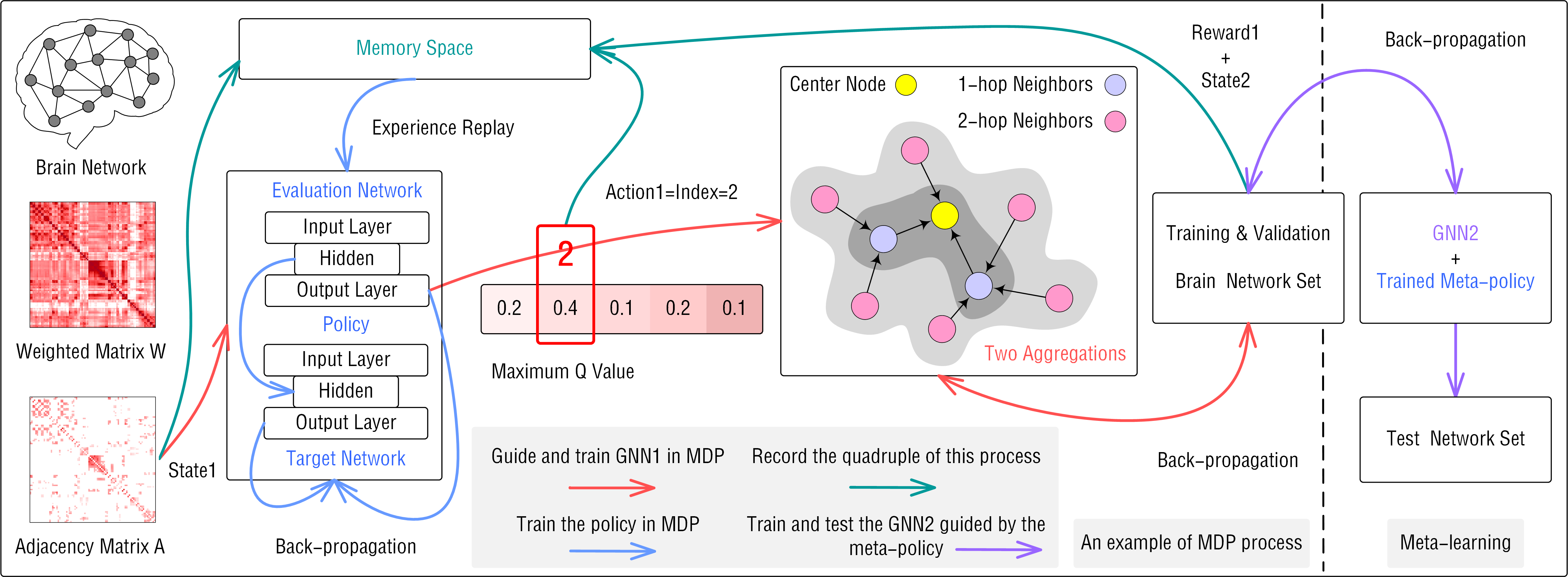
Figure 1: framework BN-GNN for brain network representation learning. The left side of the dotted line illustrates an example of the MDP process. building module as the current state and input it into the policy. Here we treat the index of the selected action in the action space as the action value to guide the number of aggregations of the current brain network in GNN. After feature aggregation, Subsequently, the current reward is calculated by comparing the performance changes on the verification set. To train the policy in MDP, we record the state-action-reward-state quadruple of this process to the memory space and follow the DDQN method to calculate the loss of the policy. On the right side of the dotted line, we apply the trained meta-policy to guide the training of a new GNN and perform brain network analysis tasks.

3.4 Solving MDP with Deep Reinforcement Learning

In many scenarios, the state space $S$ is huge or inexhaustible. In this case, it is sub-optimal or infeasible to train the policy $\pi$ by maintaining and updating a state-action table. Deep reinforcement learning (DRL) [29] is an effective solution because it can use neural networks to simulate and approximate the actual relationship between any state and all possible actions. Here, we focus on a classic DRL algorithm called double deep q-learning (DDQN) [27, 28], which uses two deep neural networks (DNNs) to simulate the policy $\pi$. Concretely, in each timestep $i$, DDQN first inputs the current state $s_{i}$ into the evaluation DNN to of all actions and regard the action corresponding to the maximum Q value as the current action, which should conform to the following formula:

$$\small\begin{split}a_{i}=\begin{cases}random\>action,&\text{w.p.}\>\epsilon\\ argmax_{a_{i}}(Q_{eval}(s_{i},a_{i})),&\text{w.p.}\>1-\epsilon\end{cases},\end{split}$$ (7)

where $\epsilon$-greedy and avoid the dilemma of exploration and utilization. The maximum Q value $max_{a_{i}}(Q(s_{i},a_{i}))$ is essentially the expected maximum discounted return in the current state $s_{i}$, and the corresponding Bellman equation can be expressed as follows:

$$\small\begin{split}max_{a_{i}}(Q_{eval}(s_{i},a_{i}))=max(\mathcal{R}_{i})&=max(r_{i}+\gamma(r_{i+1}+\gamma(r_{i+2}+\dots)))\\ &=r_{i}+\gamma max(\mathcal{R}_{i+1}).\end{split}$$ (8)

After determining the current action $a_{i}$, DDQN uses the reward function (designed according to the specific environment) to calculate the current actual reward (i.e., $r_{i}=REW(s_{i},a_{i})$) and then performs state transition to obtain the next state $s_{i+1}$. Moreover, there is a memory space in DDQN that records each MDP process (also known as “experience” and recorded as a state-action-reward-state quadruple $<s_{i},a_{i},r_{i},s_{i+1}>$). To optimize DNNs with experience replay, DDQN first records the current experience and then randomly extracts a memory block from the memory space. For example, through the experience $<s_{i},a_{i},r_{i},s_{i+1}>$, the loss of DNNs (i.e., policy) can be calculated as follows:

$$\small\begin{split}\mathcal{L}_{policy}&=(max(\mathcal{Q}_{target}(s_{i},a_{i}))-max(\mathcal{Q}_{eval}(s_{i},a_{i})))^{2}\\ &=(r_{i}+\gamma max_{a_{i+1}}(\mathcal{Q}_{target}(s_{i+1},a_{i+1}))-max_{a_{i}}(\mathcal{Q}_{eval}(s_{i},a_{i})))^{2},\end{split}$$ (9)

where state $s_{i}$ is input to the evaluation DNN to obtain the predicted maximum Q value $max_{a_{i}}(\mathcal{Q}_{eval}(s_{i},a_{i}))$ in the $i$-th timestep, the next state $s_{i+1}$ is input to the target DNN to calculate the maximum Q value $max_{a_{i+1}}(\mathcal{Q}_{target}(s_{i+1},a_{i+1})$ in the next timestep, and $r_{i}$ is the actual reword. Based on the Bellman equation, DDQN takes the $max(\mathcal{Q}_{target}(s_{i},a_{i}))$ output from the target DNN as the actual maximum Q value in timestep $i$ and trains the evaluation DNN through the back-propagation algorithm. It is worth noting that DDQN does not update the target network through loss but copies the parameters of the evaluation DNN to the target DNN. In this way, DDQN effectively alleviates the over-estimation problem often found in DRL. Since DDQN uses two DNNs to simulate the policy $\pi$, the above is also the training process of $\pi$.

4 Methodology

Fig. 1 , which consists of three modules: network building module, meta-policy module and GNN module. The network building module provides the state space for the meta-policy module. The (i.e., rewards) of the GNN module to search for the optimal meta-policy $\pi$ continuously, and the GNN module performs brain network representation learning according to the guidance (i.e., actions) of the meta-policy. Next, we introduce the technical details of each module.

4.1 Network Building Module

The network building module generates adjacency matrices from the brain networks‘ initial weighted matrices, providing state space for the meta-policy module. In GNN, should be appropriately designed to reflect the neighborhood correlations because it directly affects the node feature representation learning. Inspired by the previous work in [8], $G=(V,E)$, we utilize its weighted matrix $\mathbf{W}=\mathbf{F}^{(0)}$ and KNN to obtain reliable neighbors $V(i)$ of any node $v_{i}\in V$. If $v_{i}\in V(j)$ or $v_{j}\in V(i)$, then $\mathbf{A}(i,j)=1$ and $\mathbf{A}(j,i)=1$, otherwise . After that, we calculate new edge confidences to refine the reliable :

$$\begin{split}&\mathbf{A}(i,j)=\begin{cases}exp(-\left\|\mathbf{F}^{(0)}(i)-\mathbf{F}^{(0)}(j)\right\|),&\mathbf{A}(i,j)=1\\ 0,&\mathbf{A}(i,j)=0\end{cases},\end{split}$$ (10)

where $\mathbf{F}^{(0)}(i)$ is is also used to construct the subject network in the state transition strategy, which will be introduced in the following subsection.

4.2 Meta-policy Module

The meta-policy module trains a policy that can be viewed as meta-knowledge to determine the number of aggregations of brain network features in GNN. As mentioned in Sec. 3.3, that contains five essential components, i.e., $(S,A,\pi,REW,\mathcal{R})$. Here, we give the relevant definitions in the context of brain network embedding in timestep $i$.

$\bullet$ State space ($S$): The state $s_{i}\in S$ represents the adjacency matrix of the brain .

$\bullet$ Action space ($A$): The action $a_{i}\in A$ determines the number of iterations for feature aggregation that the brain network requires, which is reflected in the number of GNN layers. is a positive integer, we define the index of each action in the action space as the corresponding action value.

$\bullet$ Policy ($\pi$): The policy in timestep $i$ outputs action $a_{i}$ according to the input state $s_{i}$. Here we apply double deep q-network (DDQN) presented in Sec. 3.4 to simulate and train the policy and call the trained policy a meta-policy.

$\bullet$ Reward function ($REW$): The reward function outputs the reward $r_{i}$ in timestep $i$. Since we expect to improve network representation performance through policy-guided aggregations, we intuitively define the current immediate reward $r_{i}$ as the difference (a decimal) between the current validation classification performance and the performance of the previous timestep.

$\bullet$ Return ($\mathcal{R}$): The return $\mathcal{R}_{i}$ in timestep $i$ indicates the discounted accumulation of all rewards in the interval $[i,t]$. Based on the DDQN, we approximate the Q values output by the DNNs in the DDQN to the rewards over different actions. Since DDQN always chooses the action that maximizes return, it aligns with the goal of standard MDP.

According to these definitions, the process of the meta-policy module in each timestep $i$ includes five stages: 1) Sample a brain network and take its adjacency matrix as the current state $s_{i}$. 2) Determine the number of layers of the GNN that processes the current brain network according to the action $a_{i}$ corresponding to the maximum Q value output by the policy $\pi$. 3) Calculate the current reward $r_{i}$ based on performance changes (technical details will be introduced in the following subsection). 4) Obtain the next state $s_{i+1}$ with a new heuristic strategy for state transition. Concretely, we abstract the brain network of each subject as a coarse node and construct a subject network according to the network building module, where the initial node features are obtained by vectorizing the weighted matrices. Then we realize state transition through node sampling. For example, given the current state $s_{i}$ and action $a_{i}$, we randomly sample a $a_{i}$-hop neighbor of the coarse node corresponding to state $s_{i}$ in the subject’s network, corresponding to the sampled neighbor is the next state $s_{i+1}$. In this way, the state transition obeys Markov, i.e., the next state $s_{i+1}$ is only affected by the 5) Record the process of this timestep and train the policy $\pi$ according to Eq. 9 and the back-propagation algorithm.

Input: Brain network dataset $D$, number of timesteps $t$, number of all possible actions $b$, discount coefficient $\gamma$, epsilon probability $\epsilon$, window size of the history records $w$.

1:Generate adjacency matrices of brain networks and the subject network via Eq. (10), $\mathbf{A}(i,j)=exp(-\left\|\mathbf{F}^{(0)}(i)-\mathbf{F}^{(0)}(j)\right\|)$ or 0.

2:Initialize two DNNs in DDQN and two GNNs with $b$ layers.

3:Randomly sample a brain network from $D_{train}$ and get the starting state according to the adjacency matrix.

4:for $i=1,2,\dots,t$ do

5:    Select the action via Eq. (7), $a_{i}=argmax_{a_{i}}(Q_{eval}(s_{i},a_{i}))$ or a random action.

6:    Train the action value guided GNN1 in MDP via Eq. (5), $\mathcal{L}_{GNN}=-\sum_{G_{i}\in D_{train}}log(\mathbf{E}(i)\mathbf{T}^{(l+1)})\mathbf{Y}(i)^{T}$.

7:    Calculate the reward via Eq. (12), $r_{i}=REW(s_{i},a_{i})=PER(s_{i},a_{i})-\frac{1}{w}\sum_{i-w}^{i-1}PER(s_{i},a_{i})$.

8:    Sample the next state and record this process.

9:    Train the policy in MDP via Eq. (9), $\mathcal{L}_{policy}=(max(\mathcal{Q}_{target}(s_{i},a_{i}))-max(\mathcal{Q}_{eval}(s_{i},a_{i})))^{2}$.

10:end for

11:Use the trained policy, meta-policy as meta-knowledge to guide the training and testing of GNN2.

12:Obtain network representations of the test set $D_{test}$ and perform brain analysis tasks.

Algorithm 1 BN-GNN: GNN-based brain network representation learning framework

4.3 GNN Module

The GNN module contains two GNNs with a pooling layer to learn brain network representations. The first GNN (called GNN1) is used in the MDP to train the policy $\pi$. As defined in Sec. 4.2, each action is a positive integer in the interval $[1,b]$, where $b$ is the total of all possible actions. Since the action $a_{i}$ specifies the number of feature aggregations and GNN achieves different aggregations by controlling the number of layers, GNN1 needs to stack $j$ neural networks when $a_{i}=j$ ($j$ is the index of $a_{i}$ in $A$). Considering that the actions in different processes are usually different, reconstructing GNN1 in each timestep is very time- and space-consuming. To alleviate this problem, we use a parameter sharing mechanism to construct a $b$-layer GNN1. For example, given the current action $a_{i}=j$, we only use the first $j$ layers of GNN1 to learn the current brain network $G_{i}$. The aggregation process realized by  [11] is as follows:

$$\small\begin{split}\mathbf{F}^{(j)}=ReLU(\widehat{\mathbf{A}}\cdots ReLU(\widehat{\mathbf{A}}\mathbf{F}^{(0)}\mathbf{T}^{(1)})\cdots\mathbf{T}^{(j)})\end{split}.$$ (11)

After obtaining the final node feature matrix $\mathbf{F}^{(j)}$, we apply the pooling of Eq. (4) to obtain the network representation. Then we use the back-propagation algorithm of Eq. (5) to train GNN1. Since the current timestep only involves the first $b$ layers of GNN1, only the parameters of the first $b$ layers are updated. Compared with constructing a GNN for each network separately in each timestep, the parameter sharing mechanism significantly improves the training efficiency.

To calculate the current reward $r_{i}$, we measure the classification performance of GNN1 on the validation set $D_{val}$. The immediate reward as follows:

$$\small\begin{split}r_{i}=REW(s_{i},a_{i})=PER(s_{i},a_{i})-\frac{1}{w}\sum_{i-w}^{i-1}PER(s_{i},a_{i}),\end{split}$$ (12)

where $PER$ represents the performance metric of the classification result on the validation data (here we apply accuracy). $w$ indicates the number of historical records used to determine benchmark performance $\frac{1}{w}\sum_{i-w}^{i-1}PER(s_{i},a_{i})$. Compared with only considering the performance of the previous timestep $(i-1)$, the benchmark based on multiple historical performances improves the reliability of $r_{i}$.

Since the training of GNN1 and policy in MDP are usually not completed in the same timestep, it is inconvenient and inappropriate to use GNN1 to perform brain analysis tasks on the test set $D_{test}$. Therefore, after MDP, we apply the trained meta-policy to guide the training and testing of a new GNN (called GNN2), where GNN2 and GNN1 have the same aggregation type and parameter sharing mechanism. The detailed of BN-GNN is presented in Algorithm 1.

5 Experiments

(Sec. 5.1), the comparison baselines, and the experimental settings (Sec. 5.2). We then conduct sufficient experiments on the brain network classification task to

$\bullet$ RQ1. (Sec. 5.3)

$\bullet$ RQ2. Can the three modules included in BN-GNN improve brain network representations learning? (Sec. 5.4)

$\bullet$ RQ3. How do important hyperparameters in BN-GNN affect model representation performance? (Sec. 5.5)

Table 2: Statistics of Brain Network Datasets.

Dataset	BP-DTI	BP-fMRI	HIV-DTI	HIV-fMRI	ADHD-fMRI	HI-fMRI	GD-fMRI	HA-EEG
Network Instances	70	70	97	97	83	79	85	61
Healthy/Male/Active	35	35	45	45	46	44	36	21
Patient/Female/Passive	35	35	52	52	37	35	49	40
Nodes$\times$Nodes	82$\times$82	82$\times$82	90$\times$90	90$\times$90	200$\times$200	200$\times$200	200$\times$200	68$\times$68

5.1 Datasets

Table 2 shows

Human Immunodeficiency Virus Infection (HIV-DTI & HIV-fMRI): Then we obtain the corresponding weighted matrices of brain networks with 90 regions.

Bipolar Disorder (BP-DTI & BP-fMRI):  [49]. For  [50] to get the initial brain networks. Concretely, We first realign and co-register the original EPI images and then perform normalization and smoothing. For the DTI data, we follow the data processing strategy in [45] to generate brain networks whose regions are the same as those of the fMRI network.

Attention Deficit Hyperactivity Disorder (ADHD-fMRI) & Hyperactive Impulsive Disorder (HI-fMRI) & Gender (GD-fMRI): The initial data was constructed from the whole brain fMRI atlas [51]. Following the work in [52], we use the functional segmentation result CC200 from [51], which divides each . In order to explore the relationship between ROIs, we record the average value of each ROI in a specific voxel time course. Similarly, we obtain the correlation between the two ROIs according to the Pearson correlation between the two time courses, and generate three reliable brain network instance sets  [52].  [51, 52].

Hearing Activity (HA-EEG): The raw electroencephalogram (EEG) data was recorded from 61 healthy adults using 62 electrodes [53]. The participants were either actively listening to individual words over headphones (active condition) or watching a silent video and ignoring the speech (passive condition). To transform the dataset into a usable version, we perform source analysis using the fieldtrip toolkit [54] with a cortical-sheet based source model and a boundary element head model. Specifically, we calculate the coherence of all sources and segment the sources based on the 68 regions of the Desikan-Killiany cortical atlas. Furthermore, we utilize the imaginary part of the coherence spectrum as the connectivity metric to reduce the effect of electric field spread [55].

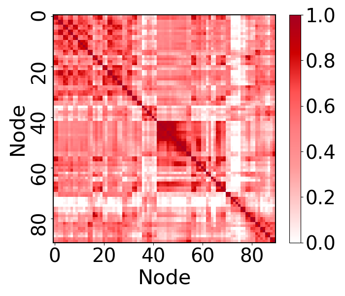
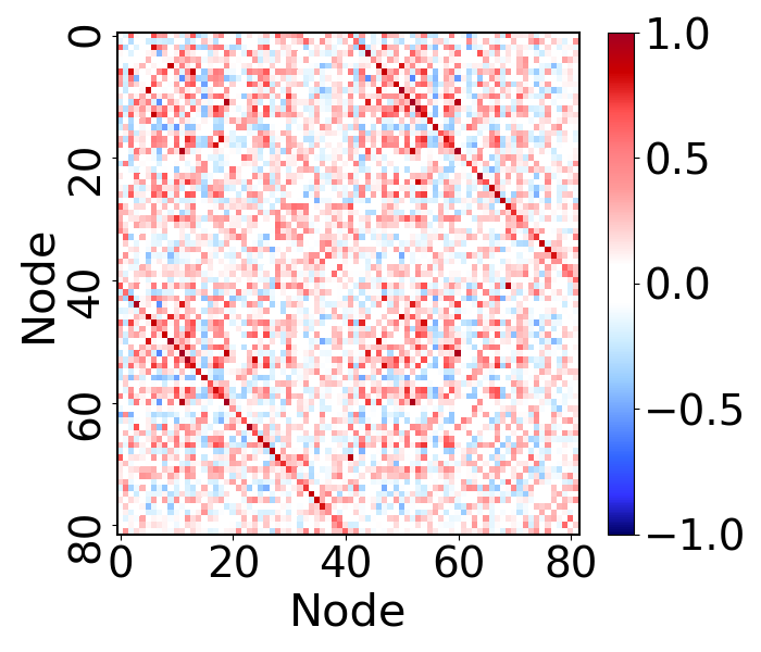
(a) Weighted matrices $\mathbf{W}$

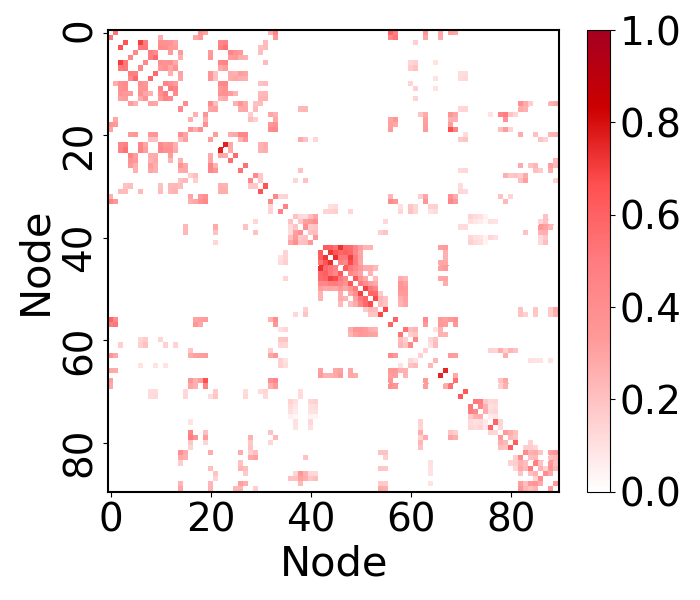
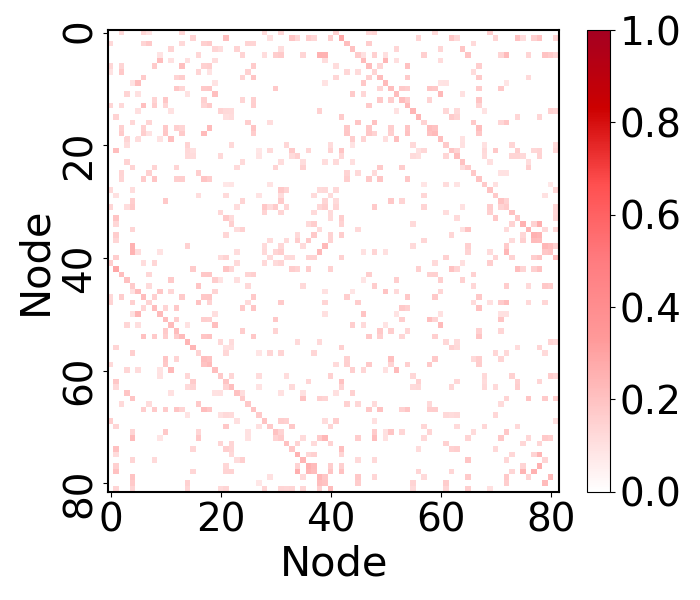
(b) Adjacency matrices $\mathbf{A}$

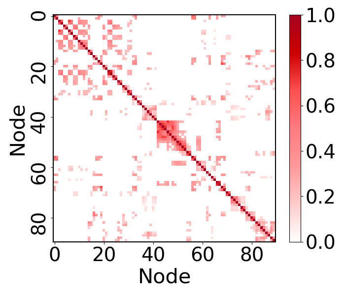
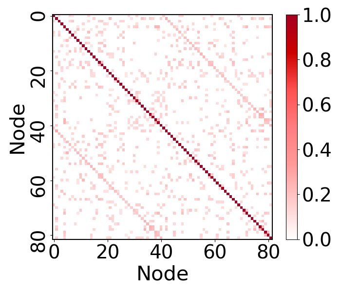
(c) Matrices with self-loop $\widetilde{\mathbf{A}}$

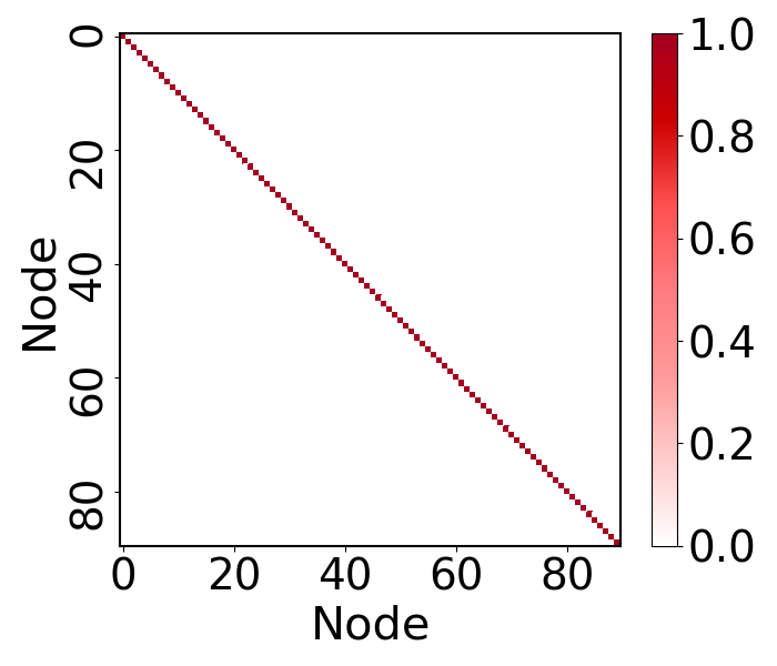
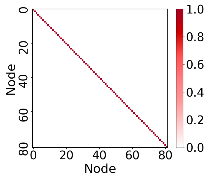
(d) Degree matrices $\mathbf{D}$

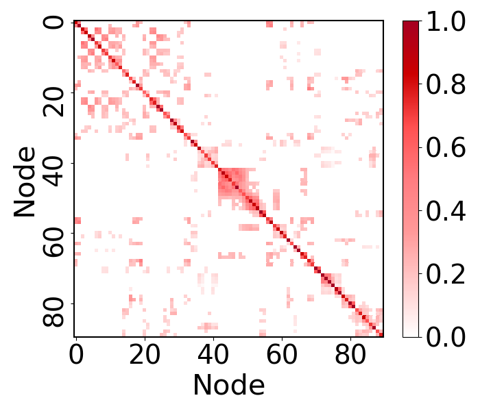
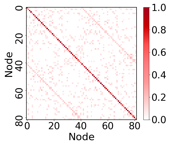
(e) Normalized matrices $\widehat{\mathbf{A}}$

Figure 2: Examples of brain networks of two subjects in fMRI modality. The subject above is from HIV, while below one is from BP. From left to right are the initial weighted matrices $\mathbf{W}$, the adjacency matrices $\mathbf{A}$ generated by the network building module (Eq. 10), and the other matrices involved in the GCN aggregation process (Eq. 2).

5.2 Baselines and Settings

DeepWalk & Node2Vec [56, 57]: The main idea of Deepwalk is to perform random walks in the network, then generate a large number of node sequences, further input these node sequences as samples into word2vec [58], and finally obtain Compared with DeepWalk, Node2Vec balances the homophily and structural equivalence of the network through biased random walks. Both of them are commonly used baselines in network representation learning.

GCN & GAT [11, 12]: Graph convolutional network (GCN) performs convolution aggregations in the graph Fourier domain, while graph attention network (GAT) performs aggregations in combination with the attention mechanism. Both of them are .

GCN+skip & GAT+skip:  [24], we construct GCN+skip and GAT+skip by adding residual skip-connections to GCN and GAT, respectively.

GraphSAGE & FastGCN [13, 59]: They are two improved GNN algorithms with different sampling strategies. For the sake of computational efficiency, GraphSAGE only samples

PR-GNN & GNEA & Hi-GCN [36, 37, 38]: Three GNN-based baselines for brain network analysis, all of which contain methods for optimizing the initial brain network generated by neuroimaging technology. PR-GNN utilizes the regularized pooling layers to filter nodes in the network and uses GAT for feature aggregation. GNEA the correlation coefficient in each brain network. Hi-GCN uses the eigenvector-based pooling layers EigenPooling to generate multiple coarse-grained sub-graphs from the initial network and then aggregates network information hierarchically and generates network representations.

SDBN [60]:

GCN and GAT, respectively, namely BN-GCN and BN-GAT. Moreover, we set the total number of timesteps $t$ to 1000, the total number of all possible actions $b$ to 3, the window size $w$ of $REW$ to 20, and the discount coefficient $\gamma$ to 0.95. For the epsilon probability $\epsilon$, we set it to decrease linearly in the first 20 timesteps, with a starting probability of 1.0 and an ending probability of 0.05. For all GNN-based methods, we use $ReLU$ with a slope of 0.2 as the activation of 0.3 between every two adjacency neural networks. For a fair comparison, we use $Adam$ optimizers with learning rates of 0.0005 and 0.005 to We set the network representation dimension of all methods to 128 and employ the strategies mentioned in the corresponding papers to adjust the parameters of with the best settings. Besides, we use the same data split ($|D_{trian}|:|D_{val}|:|D_{test}|=8:1:1$) to repeat each experiment 10 times, where each experiment records the test result with the highest verification value within 100 epochs. All experiments are performed on the same server with two 20-core CPUs (126G) and an NVIDIA Tesla P100 GPU (16G).

Table 3: on brain network classification tasks. The first part compares the experimental results of multiple methods, while the second and third parts refine the representation performance of GCNs and GATs with different layers. The bold and italicized values in each part represent the best and second-best results of all methods. $\uparrow$ indicates the improvement (%) of our BN-GNN compared to the best baseline of each part.

Method	Layers	BP-DTI	BP-fMRI	HIV-DTI	HIV-fMRI	ADHD-fMRI	HI-fMRI	GD-fMRI	HA-EEG
DeepWalk	-	0.520±0.097	0.530±0.134	0.514±0.159	0.485±0.130	0.512±0.141	0.462±0.148	0.550±0.127	0.566±0.270
Node2Vec	-	0.530±0.110	0.550±0.111	0.514±0.145	0.500±0.172	0.525±0.075	0.475±0.122	0.562±0.170	0.583±0.200
PR-GNN	2	0.590±0.186	0.630±0.110	0.557±0.174	0.585±0.100	0.625±0.167	0.600±0.165	0.600±0.145	0.650±0.157
GNEA	3	0.560±0.149	0.600±0.134	0.557±0.118	0.585±0.196	0.550±0.127	0.562±0.160	0.612±0.087	0.633±0.221
HI-GCN	3	0.540±0.162	0.600±0.109	0.528±0.192	0.571±0.127	0.562±0.128	0.562±0.160	0.587±0.148	0.616±0.183
GraphSAGE	2	0.610±0.192	0.610±0.113	0.571±0.202	0.600±0.124	0.575±0.127	0.575±0.100	0.600±0.165	0.716±0.076
FastGCN	2	0.590±0.113	0.620±0.140	0.585±0.134	0.628±0.145	0.612±0.180	0.600±0.145	0.600±0.175	0.700±0.194
BN-GNN	1$\sim$3	0.630±0.167	0.640±0.120	0.614±0.111	0.642±0.146	0.637±0.130	0.612±0.205	0.637±0.141	0.733±0.200
Gain	-	2.0$\,\uparrow$	1.0$\,\uparrow$	2.9$\,\uparrow$	1.4$\,\uparrow$	1.2$\,\uparrow$	1.2$\,\uparrow$	2.5$\,\uparrow$	1.7$\,\uparrow$
GCN	1	0.560±0.101	0.600±0.148	0.542±0.178	0.557±0.174	0.562±0.150	0.587±0.080	0.600±0.122	0.650±0.189
GCN	2	0.590±0.130	0.610±0.122	0.571±0.180	0.600±0.166	0.600±0.165	0.587±0.125	0.600±0.108	0.666±0.129
GCN	3	0.540±0.180	0.600±0.184	0.542±0.189	0.585±0.118	0.525±0.122	0.562±0.187	0.575±0.150	0.616±0.106
GCN+skip	3	0.590±0.164	0.620±0.116	0.585±0.134	0.528±0.111	0.562±0.170	0.575±0.160	0.600±0.183	0.700±0.163
BN-GCN	1$\sim$3	0.610±0.170	0.640±0.120	0.614±0.111	0.642±0.172	0.637±0.130	0.600±0.165	0.625±0.125	0.716±0.197
Gain	-	2.0$\,\uparrow$	2.0$\,\uparrow$	2.9$\,\uparrow$	4.2$\,\uparrow$	3.7$\,\uparrow$	1.3$\,\uparrow$	2.5$\,\uparrow$	1.6$\,\uparrow$
GAT	1	0.570±0.141	0.620±0.172	0.542±0.261	0.571±0.169	0.562±0.128	0.575±0.203	0.612±0.189	0.650±0.203
GAT	2	0.590±0.130	0.610±0.157	0.585±0.149	0.614±0.111	0.600±0.215	0.587±0.137	0.612±0.152	0.683±0.174
GAT	3	0.550±0.128	0.610±0.144	0.571±0.202	0.585±0.149	0.550±0.127	0.575±0.160	0.612±0.171	0.666±0.235
GAT+skip	3	0.600±0.184	0.610±0.083	0.600±0.153	0.557±0.162	0.575±0.169	0.587±0.185	0.625±0.111	0.700±0.124
BN-GAT	1$\sim$3	0.630±0.167	0.640±0.128	0.614±0.181	0.642±0.146	0.612±0.180	0.612±0.205	0.637±0.141	0.733±0.200
Gain	-	3.0$\,\uparrow$	2.0$\,\uparrow$	1.4$\,\uparrow$	2.8$\,\uparrow$	1.2$\,\uparrow$	2.5$\,\uparrow$	1.2$\,\uparrow$	3.3$\,\uparrow$

5.3 Model Comparison (RQ1)

To compare the performance of all methods, we perform disease or gender prediction (i.e., brain network classification) tasks on eight real-world datasets. Moreover, Considering that some baselines are challenging to deal with the initial weighted matrices of the brain networks that are almost complete graphs, we perform representation learning for all methods on adjacency matrices generated by the network building module. Taking GCN as an example, Fig. 2 visualizes the transformation process of the adjacency matrices of two subjects from the HIV-fMRI and BP-fMRI.

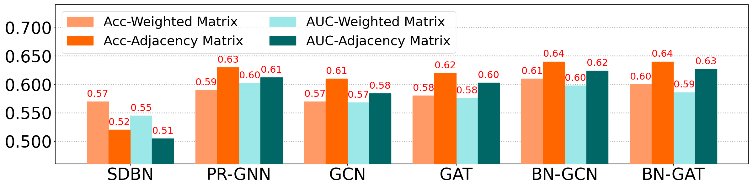
(a) BP-fMRI

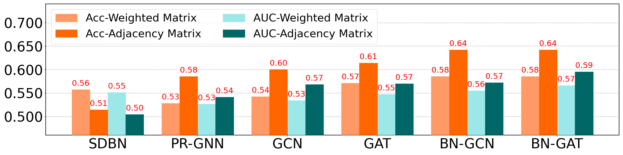
(b) HIV-fMRI

Figure 3: Visualization of ablation experiments to of the network building module on .

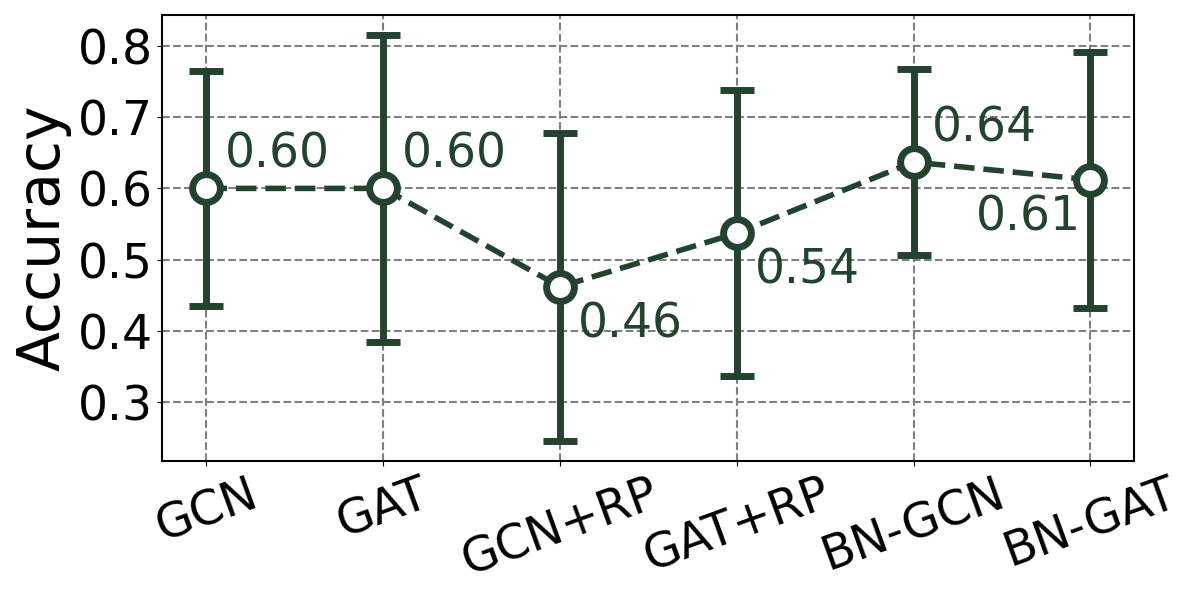
(a) ADHD-fMRI

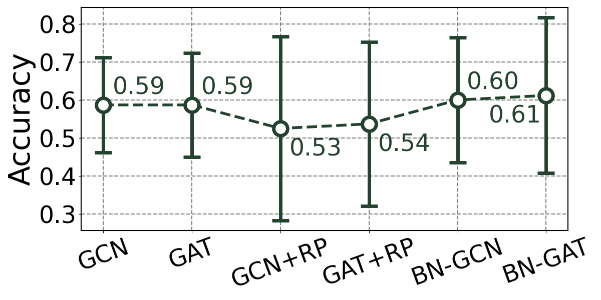
(b) HI-fMRI

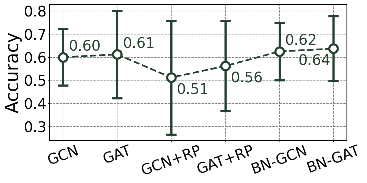
(c) GD-fMRI

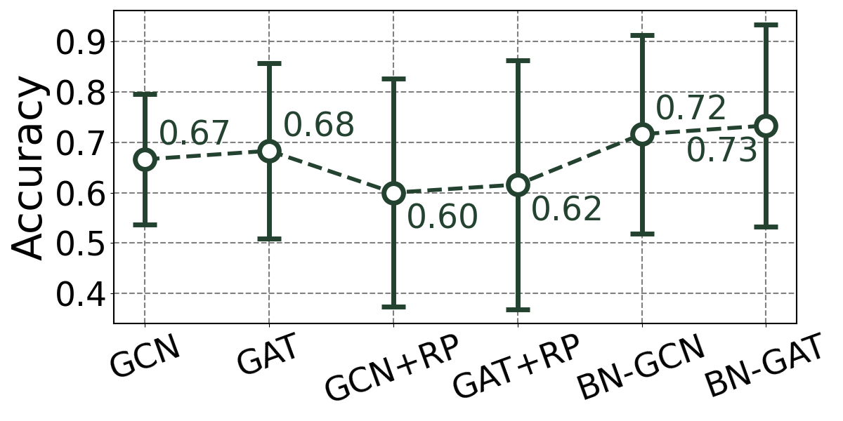
(d) HA-EEG

Figure 4: Visualization of ablation experiments to verify the performance of the meta-policy module on four datasets, where GCN+RP and GAT+RP apply a random-policy instead of the meta-policy to guide the aggregation process of GCN and GAT.

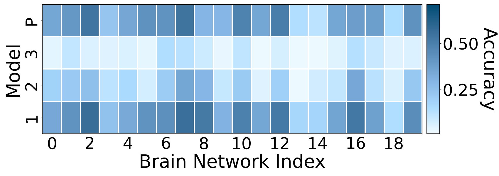
(a) Input weighted matrices $\mathbf{W}$

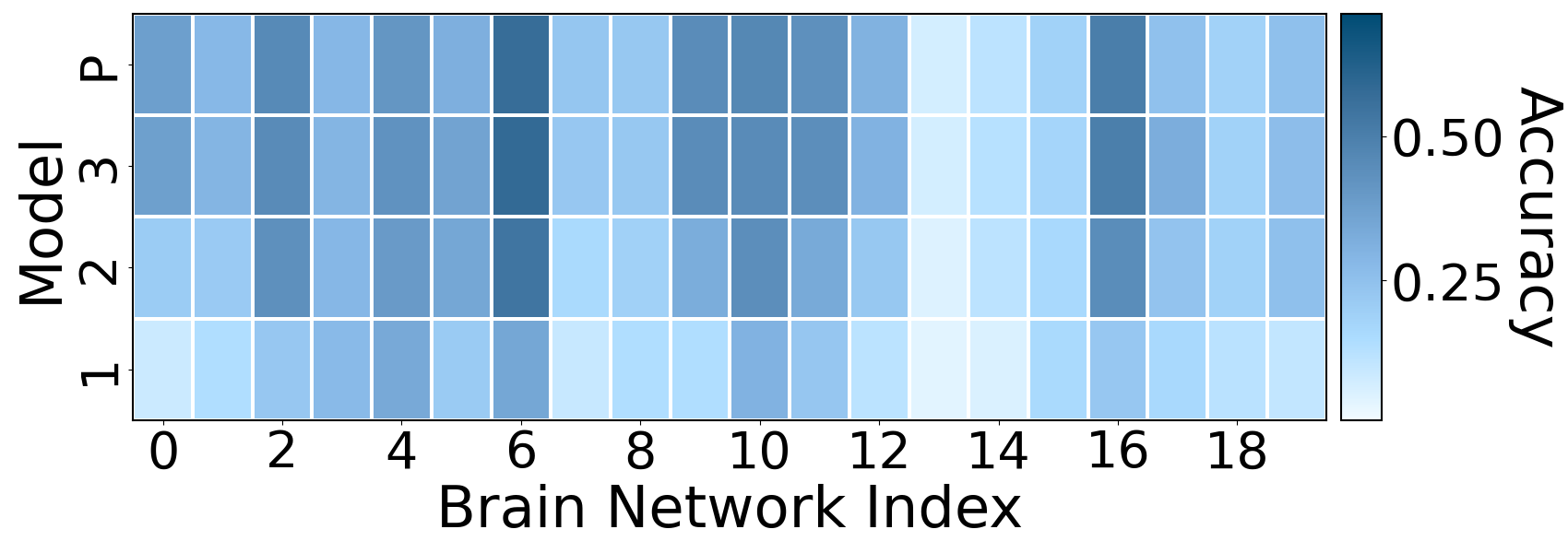
(b) Input degree matrices $\mathbf{D}$

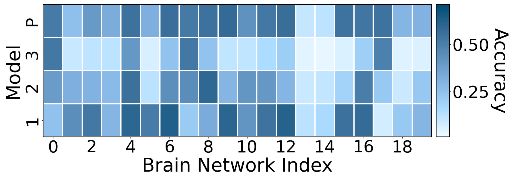
(c) Input normalized matrices $\widehat{\mathbf{A}}$

Figure 5: Visualization of classification results for 20 brain networks randomly sampled from BP-DTI, where different figures use different types of inputs/adjacency matrices. From bottom to top, the $y$-axis represents the GCN model with $y$ layers and the GCN model guided by our meta-policy. The $x$-axis represents the brain network index. The colors from light to dark mean the average accuracy from low to high.

1) BN-GNN always obtains the highest average accuracy value on all datasets, proving that its brain network representation performance is Specifically, the classification accuracy of BN-GNN on eight datasets is 2) All GNN-based methods outperform traditional network representation methods (i.e., DeepWalk and Node2Vec). This phenomenon is expected because the GNN architecture can better capture the local In addition, in brain network classification tasks, end-to-end learning strategies in brain network classification tasks are often superior to unsupervised representation learning methods. 3) GAT-based methods are generally better than GCN-based methods. Compared with the latter, the performance of the former is usually not greatly degraded. This is because the attention mechanism included in GAT alleviates the over-smoothing problem on some datasets. 4) GNNs combined with skip-connections (i.e., GCN+skip and GAT+skip) do not always enable deeper neural networks to perform better. Compared with the best GCN and GAT models have an average accuracy improvement of 2.5% and 2.1% on eight classification tasks, respectively. Although these observations reveal the limitations of skip-connections, they also confirm the hypothesis of this work that different brain networks require different aggregation iterations. In other words, since the brain networks of real subjects are usually different, customizing different GNN architectures for different subjects is essential to improve network representation performance and provide therapeutic intervention. 5) Though GraphSAGE and FastGCN improve the efficiency or structure information mining capability of the original GCN, their performance is still inferior to our BN-GNN. This phenomenon indicates that searching suitable feature aggregation strategies for network instances in brain network analysis may be more important than exploring sampling or structural reconstruction strategies.

5.4 Ablation Study (RQ2)

The classification results and analysis in Sec. 5.3 confirm the superiority of GNN-based methods in processing brain network data. Specifically, for the network building module, we compare the classification results based on the initial weighted matrices and processed adjacency matrices on BP-fMRI and HIV-fMRI, respectively. For the meta-policy module, we compare the performance of BN-GNN and random-policy-based GNN on four datasets. Furthermore, we show examples of practical use of our idea on various input types to see better how it works.

Fig. 3 visualizes the accuracy and AUC scores of ablation studies for network building, from which we 1) Utilizing the adjacency matrices generated by the network building module to replace the initial weighted matrices greatly improves the classification performance of the GNN-based methods under the two metrics. This phenomenon indicates that our proposed network building module is beneficial to promote the application of 2) The performance of SDBN on the initial matrices is better than that on the adjacency matrices. On the one hand, SDBN reconstructs the brain networks and of the initial weighted matrices, thereby enabling the CNN to capture the highly non-linear features. On the other hand, the sparse adjacency matrices generated by the network building module may not be suitable for CNN-based methods. always inferior to that of BN-GNN, indicating that it is meaningful to learn topological brain networks based on GNN. 3) Even though GAT-based methods (including PR-GNN and GAT) use the attention , they are still difficult to deal with densely connected initial brain networks. Thus, generating adjacency matrices (as shown in Fig. 2) for GNN

We replace the meta-policy module in BN-GNN with a random-policy (randomly chooses an action for a given instance) to construct the baselines of ablation experiments, namely GCN+RP and GAT+RP. Fig. 4 illustrates the results of ablation experiments for the meta-policy module, from which 1) The performance of GCN+RP and GAT+RP are worse than BN-GNN and original GNNs on ADHD-fMRI, HI-fMRI, GD-fMRI, and HA-EEG. 2) Our BN-GNN is better than the original GNNs. These phenomena once again imply that the introduction of our meta-policy can effectively improve the classification performance of brain networks.

To explore the practical application of our idea on different input types, we illustrate the classification performance of layer-fixed GCNs and GCN guided by meta-policy on BP-DTI in Fig. 5. First, we observe Fig. 5(a) and find that single-layer GCNs generally perform best when using initial weighted matrices as inputs. Besides, This may be because the initial brain networks usually have a high connection density (as shown in Fig. 2(a)), which leads to the over-smoothing problem of multi-layer GCNs during the learning process. Second, Fig. 5(b) shows the classification results with the degree matrices as inputs. Since the degree matrices do not encode neighbor information (as shown in Fig. 2(b)), these GCNs degenerate into fully-connected neural networks without feature aggregation. Therefore, the brain network classification performance of models with different numbers of layers varies relatively smoothly. Finally, after processing the initial data based on our network building module, the optimal number of GCN layers required for normalized matrices with reduced density becomes very different, as shown in Fig. 2(c). In addition, reliable brain networks improve the overall performance upper bound compared to the brain classification of the first two types of inputs. This again implies the importance of building reliable brain networks and customizing the optimal number of aggregations. In particular, our meta-policy is often able to find the optimal number of model layers corresponding to brain instances for three input types. Therefore, the GCN with our meta-policy (i.e., BN-GCN) generally performs the best (shown in the first row of subfigures in Fig. 2), even if the adjacency matrices have extremely large or small connection densities. In future research, the network building module can continue to serve brain network analysis. And the meta-policy may be extended to other scenarios with differentiated requirements for the number of model layers rather than being limited to the application of GNNs.

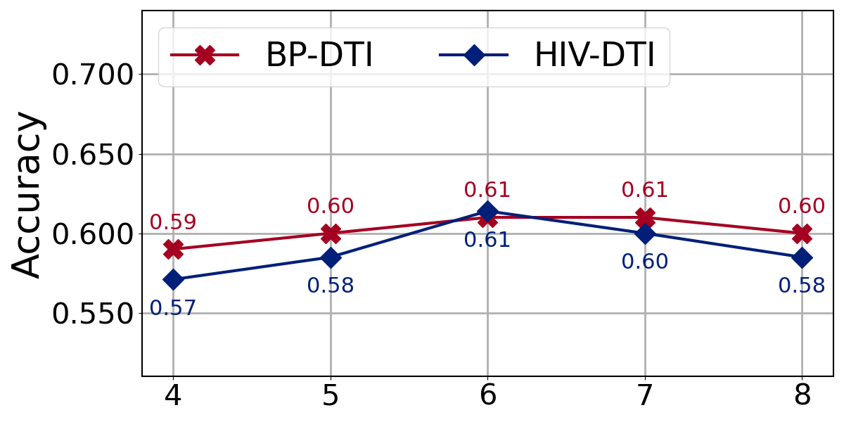
(a) Number of Neighbors

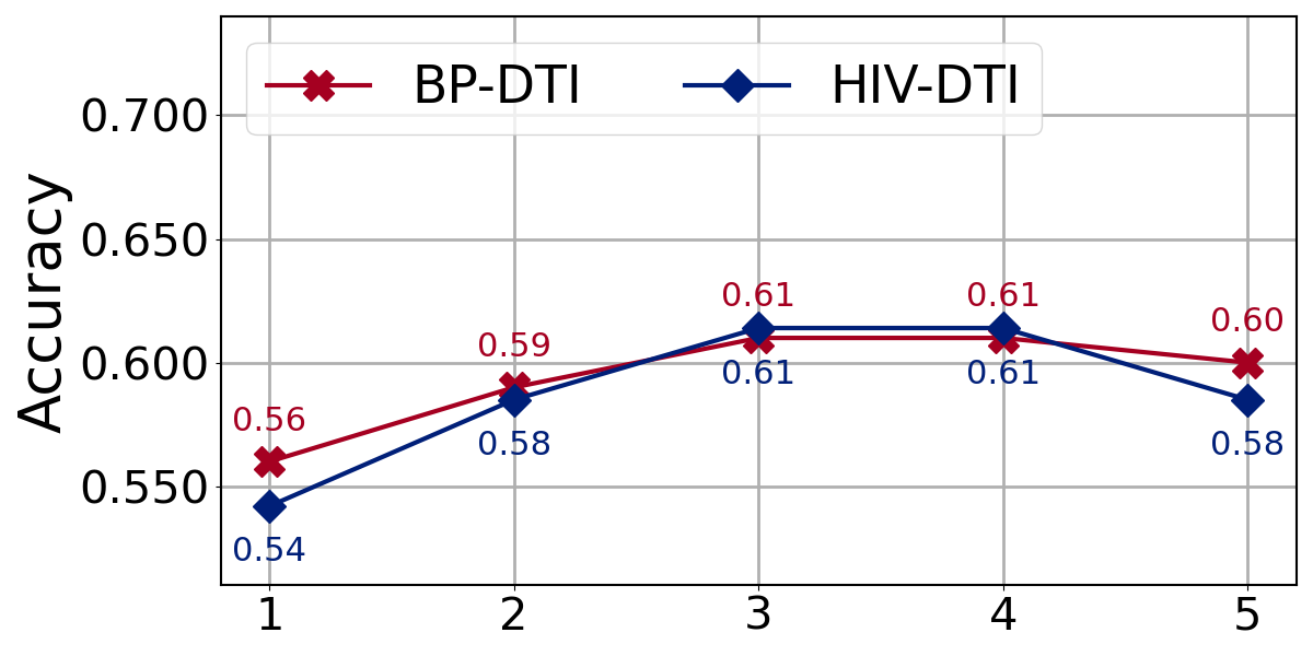
(b) Number of All Possible Actions

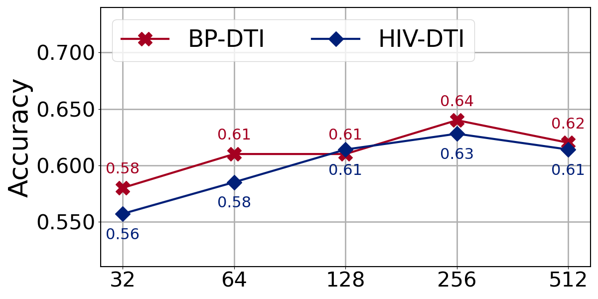
(c) Dimension of Representations

Figure 6: Hyperparameter sensitivity analysis of BN-GNN on the two datasets.

5.5 Hyperparameter Analysis (RQ3)

Fig. 6(a) shows that increasing the number of neighbors (determined by k of KNN) when building the adjacency matrix does not always yield better network representations. The possible reason is that each region in the brain network only has meaningful connections with a limited number of neighbors. From Fig. 6(b), we observe that the performance of BN-GNN is often the best when the number of aggregations is 3. When the action space is further expanded, BN-GNN still maintains a relatively stable performance. These two phenomena verify that the best representation of most brain networks can be obtained within 3 aggregations, and BN-GNN is robust to . The results in Fig. 6(c) show that unless the dimension is too small, the performance of BN-GNN will not

6 Conclusions and Future Work

to achieve customized aggregation for different networks, effectively improving traditional GNNs in brain network representation learning. Experimental results In future work, we will improve BN-GNN from both technical and practical aspects. Technically, we discuss the idea of automatically searching hyperparameters for our model BN-GNN as a future trend. Practically, we state the explainability of our model, which is an emerging area in brain network analysis. Specifically, even if we observe that changes in the number of neighbors have little effect on the performance of BN-GNN, setting this hyperparameter manually is not an optimal solution. Therefore, multi-agent reinforcement learning can be introduced into BN-GNN to automatically search for the optimal brain network structure and model layer number. the explainability of the classification results is often as important as the accuracy. In other words, while successfully predicting a damaged brain network, it is also necessary to understand which regions within the network are responsible for the damage. Therefore, to improve the explainability, attention-based pooling and grad-cam, can be introduced to BN-GNN.

Declaration of Competing Interest

The authors declare that they have no known competing financial interests or personal relationships that could have appeared to influence the work reported in this paper.

References

- Alexander et al. [2007] A. L. Alexander, J. E. Lee, M. Lazar, A. S. Field, Diffusion tensor imaging of the brain, Neurotherapeutics 4 (2007) 316–329.
- Huettel et al. [2004] S. A. Huettel, A. W. Song, G. McCarthy, et al., Functional magnetic resonance imaging, volume 1, Sinauer Associates Sunderland, MA, 2004.
- Van Den Heuvel and Pol [2010] M. P. Van Den Heuvel, H. E. H. Pol, Exploring the brain network: A review on resting-state fmri functional connectivity, European Neuropsychopharmacology 20 (2010) 519–534.
- Urbanski et al. [2008] M. Urbanski, M. T. De Schotten, S. Rodrigo, et al., Brain networks of spatial awareness: Evidence from diffusion tensor imaging tractography, Journal of Neurology Neurosurgery and Psychiatry 79 (2008) 598–601.
- Liu et al. [2018] Y. Liu, L. He, B. Cao, P. S. Yu, A. B. Ragin, A. D. Leow, Multi-view multi-graph embedding for brain network clustering analysis, in: Proceedings of the AAAI Conference on Artificial Intelligence, volume 32, AAAI Press, 2018, pp. 117–124.
- Parisot et al. [2018] S. Parisot, S. I. Ktena, E. Ferrante, M. Lee, R. Guerrero, B. Glocker, D. Rueckert, Disease prediction using graph convolutional networks: Application to autism spectrum disorder and alzheimer’s disease, Medical Image Analysis 48 (2018) 117–130.
- Braak and Braak [1991] H. Braak, E. Braak, Neuropathological stageing of alzheimer-related changes, Acta Neuropathologica 82 (1991) 239–259.
- Zhang et al. [2018] X. Zhang, L. He, K. Chen, Y. Luo, J. Zhou, F. Wang, Multi-view graph convolutional network and its applications on neuroimage analysis for parkinson’s disease, in: AMIA Annual Symposium Proceedings, volume 2018, American Medical Informatics Association, 2018, pp. 1147–1156.
- Huang and Mucke [2012] Y. Huang, L. Mucke, Alzheimer mechanisms and therapeutic strategies, Cell 148 (2012) 1204–1222.
- Cao et al. [2017] B. Cao, L. He, X. Wei, M. Xing, P. S. Yu, H. Klumpp, A. D. Leow, t-bne: Tensor-based brain network embedding, in: International Conference on Data Mining, SIAM, 2017, pp. 189–197.
- Kipf and Welling [2017] T. N. Kipf, M. Welling, Semi-supervised classification with graph convolutional networks, in: International Conference on Learning Representations, 2017.
- Velickovic et al. [2018] P. Velickovic, G. Cucurull, A. Casanova, A. Romero, P. Lio, Y. Bengio, Graph attention networks, in: International Conference on Learning Representations, 2018.
- Hamilton et al. [2017] W. L. Hamilton, Z. Ying, J. Leskovec, Inductive representation learning on large graphs, in: NeurIPS, 2017, pp. 1025–1035.
- Peng et al. [2020] H. Peng, J. Li, Q. Gong, Y. Ning, S. Wang, L. He, Motif-matching based subgraph-level attentional convolutional network for graph classification, in: Proceedings of the AAAI Conference on Artificial Intelligence, volume 34, 2020, pp. 5387–5394.
- Sun et al. [2021] Q. Sun, J. Li, H. Peng, J. Wu, Y. Ning, P. S. Yu, L. He, Sugar: Subgraph neural network with reinforcement pooling and self-supervised mutual information mechanism, in: Proceedings of the Web Conference, 2021, pp. 2081–2091.
- LeCun et al. [2015] Y. LeCun, Y. Bengio, G. Hinton, Deep learning, Nature 521 (2015) 436–444.
- Ma et al. [2021] X. Ma, J. Wu, S. Xue, J. Yang, C. Zhou, Q. Z. Sheng, H. Xiong, L. Akoglu, A comprehensive survey on graph anomaly detection with deep learning, IEEE Transactions on Knowledge and Data Engineering (2021).
- Liu et al. [2020] F. Liu, S. Xue, J. Wu, C. Zhou, W. Hu, C. Paris, S. Nepal, J. Yang, P. S. Yu, Deep learning for community detection: Progress, challenges and opportunities, in: International Joint Conference on Artificial Intelligence, 2020, pp. 4981–4987.
- Arslan et al. [2018] S. Arslan, S. I. Ktena, B. Glocker, D. Rueckert, Graph saliency maps through spectral convolutional networks: Application to sex classification with brain connectivity, in: Graphs in Biomedical Image Analysis and Integrating Medical Imaging and Non-Imaging Modalities, Springer, 2018, pp. 3–13.
- Ktena et al. [2018] S. I. Ktena, S. Parisot, E. Ferrante, M. Rajchl, M. Lee, B. Glocker, D. Rueckert, Metric learning with spectral graph convolutions on brain connectivity networks, NeuroImage 169 (2018) 431–442.
- Oono and Suzuki [2019] K. Oono, T. Suzuki, Graph neural networks exponentially lose expressive power for node classification, in: International Conference on Learning Representations, 2019.
- Chen et al. [2020] D. Chen, Y. Lin, W. Li, P. Li, J. Zhou, X. Sun, Measuring and relieving the over-smoothing problem for graph neural networks from the topological view, in: Proceedings of the AAAI Conference on Artificial Intelligence, volume 34, 2020, pp. 3438–3445.
- Gao and Ji [2019] H. Gao, S. Ji, Graph u-nets, in: International Conference on Machine Learning, PMLR, 2019, pp. 2083–2092.
- Li et al. [2019] G. Li, M. Muller, A. Thabet, B. Ghanem, Deepgcns: Can gcns go as deep as cnns?, in: Proceedings of the IEEE/CVF International Conference on Computer Vision, 2019, pp. 9267–9276.
- Lai et al. [2020] K.-H. Lai, D. Zha, K. Zhou, X. Hu, Policy-gnn: Aggregation optimization for graph neural networks, in: Proceedings of the ACM SIGKDD International Conference on Knowledge Discovery Data Mining, 2020, pp. 461–471.
- Zha et al. [2019] D. Zha, K.-H. Lai, K. Zhou, X. Hu, Experience replay optimization, in: International Joint Conference on Artificial Intelligence, 2019.
- Mnih et al. [2015] V. Mnih, K. Kavukcuoglu, D. Silver, A. A. Rusu, J. Veness, M. G. Bellemare, A. Graves, M. Riedmiller, A. K. Fidjeland, G. Ostrovski, et al., Human-level control through deep reinforcement learning, Nature 518 (2015) 529–533.
- Van Hasselt et al. [2016] H. Van Hasselt, A. Guez, D. Silver, Deep reinforcement learning with double q-learning, in: Proceedings of the AAAI Conference on Artificial Intelligence, volume 30, 2016.
- Arulkumaran et al. [2017] K. Arulkumaran, M. P. Deisenroth, M. Brundage, A. A. Bharath, Deep reinforcement learning: A brief survey, IEEE Signal Processing Magazine 34 (2017) 26–38.
- Dou et al. [2020] Y. Dou, Z. Liu, L. Sun, Y. Deng, H. Peng, P. S. Yu, Enhancing graph neural network-based fraud detectors against camouflaged fraudsters, in: Proceedings of the ACM International Conference on Information Knowledge Management, 2020, pp. 315–324.
- Peng et al. [2021] H. Peng, R. Zhang, Y. Dou, R. Yang, J. Zhang, P. S. Yu, Reinforced neighborhood selection guided multi-relational graph neural networks, ACM Transactions on Information Systems (2021) 1–46.
- Peng et al. [2022] H. Peng, R. Zhang, S. Li, Y. Cao, S. Pan, P. Yu, Reinforced, incremental and cross-lingual event detection from social messages, IEEE Transactions on Pattern Analysis and Machine Intelligence (2022) 1–1.
- Gao et al. [2020] Y. Gao, H. Yang, P. Zhang, C. Zhou, Y. Hu, Graph neural architecture search., in: International Joint Conference on Artificial Intelligence, volume 20, 2020, pp. 1403–1409.
- Nishi et al. [2018] T. Nishi, K. Otaki, K. Hayakawa, T. Yoshimura, Traffic signal control based on reinforcement learning with graph convolutional neural nets, in: International Conference on Intelligent Transportation Systems, IEEE, 2018, pp. 877–883.
- Yan et al. [2020] Z. Yan, J. Ge, Y. Wu, L. Li, T. Li, Automatic virtual network embedding: A deep reinforcement learning approach with graph convolutional networks, IEEE Journal on Selected Areas in Communications 38 (2020) 1040–1057.
- Li et al. [2020] X. Li, Y. Zhou, N. C. Dvornek, M. Zhang, J. Zhuang, P. Ventola, J. S. Duncan, Pooling regularized graph neural network for fmri biomarker analysis, in: International Conference on Medical Image Computing and Computer-Assisted Intervention, Springer, 2020, pp. 625–635.
- Bi et al. [2020] X. Bi, Z. Liu, Y. He, X. Zhao, Y. Sun, H. Liu, Gnea: A graph neural network with elm aggregator for brain network classification, Complexity 2020 (2020).
- Jiang et al. [2020] H. Jiang, P. Cao, M. Xu, J. Yang, O. Zaiane, Hi-gcn: A hierarchical graph convolution network for graph embedding learning of brain network and brain disorders prediction, Computers in Biology and Medicine 127 (2020) 104096.
- Ma et al. [2019] G. Ma, N. K. Ahmed, T. L. Willke, D. Sengupta, M. W. Cole, N. B. Turk-Browne, P. S. Yu, Deep graph similarity learning for brain data analysis, in: Proceedings of the ACM International Conference on Information and Knowledge Management, 2019, pp. 2743–2751.
- Zhong et al. [2020] P. Zhong, D. Wang, C. Miao, Eeg-based emotion recognition using regularized graph neural networks, IEEE Transactions on Affective Computing (2020) 1–1.
- Xing et al. [2021] X. Xing, Q. Li, M. Yuan, H. Wei, Z. Xue, T. Wang, F. Shi, D. Shen, Ds-gcns: Connectome classification using dynamic spectral graph convolution networks with assistant task training, Cerebral Cortex 31 (2021) 1259–1269.
- Gurbuz and Rekik [2021] M. B. Gurbuz, I. Rekik, Mgn-net: A multi-view graph normalizer for integrating heterogeneous biological network populations, Medical Image Analysis 71 (2021) 102059.
- Zhang and Huang [2019] Y. Zhang, H. Huang, New graph-blind convolutional network for brain connectome data analysis, in: International Conference on Information Processing in Medical Imaging, Springer, 2019, pp. 669–681.
- Ragin et al. [2012] A. B. Ragin, H. Du, R. Ochs, Y. Wu, C. L. Sammet, A. Shoukry, L. G. Epstein, Structural brain alterations can be detected early in hiv infection, Neurology 79 (2012) 2328–2334.
- Ma et al. [2017] G. Ma, L. He, C.-T. Lu, W. Shao, P. S. Yu, A. D. Leow, A. B. Ragin, Multi-view clustering with graph embedding for connectome analysis, in: Proceedings of the ACM International Conference on Information Knowledge Management, 2017, pp. 127–136.
- Yan and Zang [2010] C. Yan, Y. Zang, Dparsf: A matlab toolbox for ”pipeline” data analysis of resting-state fmri, Frontiers in systems neuroscience 4 (2010) 13.
- Tzourio-Mazoyer et al. [2002] N. Tzourio-Mazoyer, B. Landeau, D. Papathanassiou, F. Crivello, O. Etard, N. Delcroix, B. Mazoyer, M. Joliot, Automated anatomical labeling of activations in spm using a macroscopic anatomical parcellation of the mni mri single-subject brain, Neuroimage 15 (2002) 273–289.
- Smith et al. [2004] S. M. Smith, M. Jenkinson, M. W. Woolrich, C. F. Beckmann, T. E. Behrens, H. Johansen-Berg, P. R. Bannister, M. De Luca, I. Drobnjak, D. E. Flitney, et al., Advances in functional and structural mr image analysis and implementation as fsl, Neuroimage 23 (2004) S208–S219.
- Cao et al. [2015] B. Cao, L. Zhan, X. Kong, P. S. Yu, N. Vizueta, L. L. Altshuler, A. D. Leow, Identification of discriminative subgraph patterns in fmri brain networks in bipolar affective disorder, in: International Conference on Brain Informatics and Health, Springer, 2015, pp. 105–114.
- Whitfield-Gabrieli and Nieto-Castanon [2012] S. Whitfield-Gabrieli, A. Nieto-Castanon, Conn: A functional connectivity toolbox for correlated and anticorrelated brain networks, Brain Connectivity 2 (2012) 125–141.
- Craddock et al. [2012] R. C. Craddock, G. A. James, P. E. Holtzheimer III, X. P. Hu, H. S. Mayberg, A whole brain fmri atlas generated via spatially constrained spectral clustering, Human Brain Mapping 33 (2012) 1914–1928.
- Pan et al. [2016] S. Pan, J. Wu, X. Zhu, G. Long, C. Zhang, Task sensitive feature exploration and learning for multitask graph classification, IEEE Transactions on Cybernetics 47 (2016) 744–758.
- Hernandez-Perez et al. [2021] H. Hernandez-Perez, J. Mikiel-Hunter, D. McAlpine, S. Dhar, S. Boothalingam, J. J. Monaghan, C. M. McMahon, Perceptual gating of a brainstem reflex facilitates speech understanding in human listeners, bioRxiv (2021) 2020–05.
- Oostenveld et al. [2011] R. Oostenveld, P. Fries, E. Maris, J.-M. Schoffelen, Fieldtrip: Open source software for advanced analysis of meg, eeg, and invasive electrophysiological data, Computational Intelligence and Neuroscience 2011 (2011).
- Nolte et al. [2004] G. Nolte, O. Bai, L. Wheaton, Z. Mari, S. Vorbach, M. Hallett, Identifying true brain interaction from eeg data using the imaginary part of coherency, Clinical Neurophysiology 115 (2004) 2292–2307.
- Perozzi et al. [2014] B. Perozzi, R. Al-Rfou, S. Skiena, Deepwalk: Online learning of social representations, in: Proceedings of the ACM SIGKDD International Conference on Knowledge Discovery Data Mining, 2014, pp. 701–710.
- Grover and Leskovec [2016] A. Grover, J. Leskovec, Node2vec: Scalable feature learning for networks, in: Proceedings of the ACM SIGKDD International Conference on Knowledge Discovery Data Mining, 2016, pp. 855–864.
- Mikolov et al. [2013] T. Mikolov, K. Chen, G. Corrado, J. Dean, Efficient estimation of word representations in vector space, in: International Conference on Learning Representations, 2013.
- Chen et al. [2018] J. Chen, T. Ma, C. Xiao, Fastgcn: Fast learning with graph convolutional networks via importance sampling, in: International Conference on Learning Representations, 2018.
- Wang et al. [2017] S. Wang, L. He, B. Cao, C.-T. Lu, P. S. Yu, A. B. Ragin, Structural deep brain network mining, in: Proceedings of the ACM SIGKDD International Conference on Knowledge Discovery Data Mining, 2017, pp. 475–484.
- Krizhevsky et al. [2012] A. Krizhevsky, I. Sutskever, G. E. Hinton, Imagenet classification with deep convolutional neural networks, Advances in Neural Information Processing Systems 25 (2012) 1097–1105.