Quantum anomalous Hall effect and electric-field-induced topological phase transition in AB-stacked MoTe₂/WSe₂ moiré heterobilayers

Abstract

We propose a new mechanism to explain the quantum anomalous Hall (QAH) effect and the electric-field-induced topological phase transition in AB-stacked MoTe₂/WSe₂ moiré heterobilayers at $\nu=1$ hole filling. We suggest that the Chern band of the QAH state is generated from an intrinsic band inversion composed of the highest two moiré hole bands with opposite valley numbers and a gap opening induced by two Coulomb-interaction-driven magnetic orders. These magnetic orders, including an in-plane $120^{\circ}$-Néel order and an in-plane ferromagnetic order, interact with moiré bands via corresponding in-plane exchange fields. The Néel order ensures the insulating gap, the ferromagnetic order induces the non-zero Chern number, and both orders contribute to time-reversal symmetry (TRS) breaking. The Néel order is acquired from the Hartree-Fock exchange interaction, and the formation of ferromagnetic order is attributed to interlayer-exciton condensation and exciton ferromagnetism. The exciton ferromagnetism can be demonstrated by excitonic Bose-Hubbard physics and Berezinskii-Kosterlitz-Thouless (BKT) transition. In low electric fields, the equilibrium state is a Mott-insulator state. At a certain electric field, a correlated insulating state composed of the hole-occupied band and the exciton condensate becomes a new thermodynamically stable phase, and the topological phase transition occurs as the ferromagnetic order emerges. The consistency between the present theory and experimental observations is discussed. Experimental observations, including the spin-polarized/valley-coherent nature of the QAH state, the absence of charge gap closure at the topological phase transition, the canted spin texture, and the insulator-to-metal transition, are interpreted by the mechanism.

I Introduction

Recently, quantum anomalous Hall (QAH) insulators and related topological materials have drawn a lot of attention from scientists for their fundamental importance and potential to design quantum deviceskonig2008quantum ; bernevig2013topological ; hohenadler2013correlation ; weng2015quantum ; liu2016quantum . A QAH (insulating) state is a two-dimensional insulator that carries a chiral edge state exhibiting a quantized Hall conductance in the unit of $e^{2}/h$, and the quantum Hall conductance along with zero longitudinal resistance in the absence of an external magnetic field is known as the QAH effectbernevig2013topological ; hohenadler2013correlation ; weng2015quantum ; liu2016quantum . Moiré material is a new platform for studying the QAH effectchen2020tunable ; serlin2020intrinsic ; tschirhart2021imaging ; zhang2019nearly ; wu2019topological . Recently, a QAH state in AB-stacked MoTe₂/WSe₂ moiré heterobilayers and an electric-field-induced topological phase transition were observed at $\nu=1$ hole filling under an out-of-plane electric fieldexp0 ; exp1 ; exp2 . Some experimental observations, such as the spin-polarized/valley-coherent nature of the QAH stateexp1 and the absence of charge gap closure at the topological phase transitionexp0 , are unique among related materials. Several theories have been proposed to explain the mechanism and observationstheory1 ; theory2 ; theory3 ; theory4 ; theory5 ; theory6 ; theory7 ; theory8 ; theory9 , but some questions remain.

A suitable theory to explain the QAH effect in AB-stacked MoTe₂/WSe₂ heterobilayers should meet certain theoretical criteria and be able to explain related experimental observations. Theoretically, for an insulator exhibiting the QAH effect, it must contain at least an occupied band that is topological non-trivial and carries a non-zero Chern number (i.e. a Chern band), and time-reversal symmetry (TRS) of the insulator must be brokenbernevig2013topological ; hohenadler2013correlation ; weng2015quantum ; liu2016quantum . Experimentally, in addition to the QAH effect, AB-stacked MoTe₂/WSe₂ heterobilayers also show the following properties:

1. At a small electric field and $\nu=1$ hole filling, the longitudinal resistance diverges rapidly as temperature decreases, indicating a Mott-insulator stateexp0 .

2. The MoTe₂ valence band maximum is about $300$ meV above the WSe₂ valence band maximum in the absence of an electric field. A topological phase transition between a topological trivial insulating state and the QAH state occurs at $\nu=1$ hole filling as the electric field contributes about $-172$ meV shift (with $0.66$ V/nm electric-field strength and $2.6$ e$\cdot$Å  interlayer dipole momentli2021continuous ) to the valence-band energy offset. However, no charge gap closure is found at the transitionexp0 .

3. The magnetic-field dependence of transverse resistances of the QAH state was studied. A magnetic hysteresis with a sharp magnetic switching in low temperature was observed, and the onset of magnetic ordering is at approximately $5\sim 6$ Kexp0 .

4. The charge gap of the insulating state decreases continuously as the electric field increases. An insulator-to-metal transition occurs as the electric-field strength reaches $0.70$ V/nm. The metallic state seems to follow a Fermi liquid behavior at low temperatures and converges to a finite resistance in the zero-temperature limitexp0 .

5. The relative alignment of the spontaneous spin (valley) polarization in the moiré heterobilayer in the QAH state was studied by the magnetic circular dichroism (MCD) of the attractive polaron feature in each layer. It was found that the QAH ground state is consistent with a spin-polarized/valley-coherent state across two layers, in which the spin polarization is alignedexp1 .

6. The magnetic-field dependence of the out-of-plane spin polarization was also studied by the MCD. The maximum MCD signals in both layers increase monotonically with increasing magnetic fields until saturating, as the transverse resistance is quantized near zero magnetic field and does not depend on the magnetic field. It implies that full spin polarization is not necessary for quantized Hall transport, and a canted spin texture could existexp1 .

7. Evidence of quantum spin Hall (QSH) effect was observed at $\nu=2$ hole filling. A band-to-QSH insulator transition occurs at $-130$ meV energy shift ($0.50$ V/nm electric-field strength), and charge gap closure and reopening were foundexp0 ; exp2 .

In addition to these experimental observations in AB-stacked MoTe₂/WSe₂ heterobilayers, a continuous Mott transition is observed in AA-stacked MoTe₂/WSe₂ heterobilayers at $\nu=1$ hole filling, but no QAH effect or QSH effect is foundli2021continuous . Some theoretical works have explained some of these properties, but a theory consistent with all experimental observations is still elusive.

A critical issue of the QAH effect in the present system is the mechanism of electric-field-induced topological phase transition at $\nu=1$ filling. The topological phase transition bridges a topological trivial insulating state and the QAH insulating state. Theoretical works to study the QAH effect are supposed to propose a mechanism to explain the transition. In Ref. theory2 ; theory4 ; theory5 ; theory6 , the topological phase transition is explained by a band-inversion mechanism involving Coulomb interaction and interlayer tunneling. Based on this mechanism, a band inversion between the moiré bands at the MoTe₂ layer and the WSe₂ layer occurs due to electric-field-induced band-energy shift. A topological gap is opened by interlayer tunneling. The TRS is broken by a Coulomb-interaction-driven valley polarization of holes. A hole-occupied and valley-polarized Chern band is formed, and the topological phase transition occurs. In Ref. theory7 ; theory8 ; theory9 , the band inversion between the moiré bands at different layers is also induced by the electric field, but the gap opening here is induced by Coulomb-interaction-driven topological exciton condensation. The exciton condensate is a spin-polarized/valley-coherent state, and it also contributes to the TRS breaking. The topological gap is opened and a hole-occupied Chern band is formed via an inter-band exchange interaction induced by the exciton condensate. In Ref. theory1 , the Chern band is generated by geometry-relaxation-induced pseudo-magnetic field and intrinsic band inversion. The TRS is broken and the topological phase transition occurs due to the interaction-driven valley polarization. In Ref. theory3 , the moiré band structure is studied by the model of a Dirac hole quasiparticle in a moiré potential. The Chern band is formed and the topological phase transition occurs due to an electric-field-induced phase-angle tuning for the moiré potential. The TRS is also broken by the interaction-driven valley polarization.

For mechanisms proposed by Ref. theory2 ; theory4 ; theory5 ; theory6 ; theory7 ; theory8 ; theory9 , the electric-field-induced band inversion involves a charge gap closure and reopeningweng2015quantum , yet it is not consistent with the observation of the absence of charge gap closure. For mechanisms proposed by Ref. theory1 ; theory3 , the electric-field-induced band inversion is no longer required, but the spin-polarized/valley-coherent state observed in the QAH insulator is not explained. Besides, there is still no widely accepted explanation for the insulator-to-metal transition or the canted spin texture.

In this article, a new mechanism for explaining the QAH state and the topological phase transition in AB-stacked MoTe₂/WSe₂ heterobilayers is proposed. The Chern band is generated from an intrinsic band inversion and a gap opening. The intrinsic band inversion is composed of the highest two moiré hole bands with opposite valley numbers. The gap opening is induced by two Coulomb-interaction-driven magnetic orders, an in-plane $120^{\circ}$-Néel order and an in-plane ferromagnetic order. The Néel order ensures the insulating gap, the ferromagnetic order induces the non-zero Chern number, and both orders contribute to TRS breaking. The Néel order is acquired from the Hartree-Fock exchange interaction, and the ferromagnetic order is attributed to interlayer-exciton condensation. In low electric fields, the equilibrium state is a Mott-insulator state. At a certain electric field, a correlated insulating state composed of the hole-occupied band and the exciton condensate becomes a new thermodynamically stable phase, and the topological phase transition occurs as the ferromagnetic order emerges. Since the band inversion is intrinsic and the gap is opened before the topological phase transition, there is no charge gap closure. The QAH state being spin-polarized/valley-coherent across two layers is consistent with the interlayer exciton condensate. The insulator-to-metal transition can be interpreted as an exciton Mott transition. The canted spin texture is attributed to a coexistence of the Néel order and field-induced valley polarization of holes. In Sec. II, the continuum model for the moiré heterobilayers under magnetic and exchange fields is introduced, and the symmetry is discussed. In Sec. III, the origin of Chern bands in the moiré heterobilayers is studied. Effects of in-plane Néel order, in-plane ferromagnetic order, and field-induced valley polarization on moiré bands are discussed. In Sec. IV, the concepts of interlayer-exciton condensation, exciton ferromagnetism, and exciton Mott transition are introduced. Finally, in Sec. V, the consistency between the theory and experimental observations is discussed. Derivations and formulations for studying moiré band structures and exciton condensation are given in Appendix A and Appendix B.

II Moiré superlattice

In this section, the geometry, model, symmetry, and band structure of AB-stacked MoTe₂/WSe₂ heterobilayers are introduced. In Sec. II.1, the moiré superlattice and the moiré reciprocal lattice are introduced. In Sec. II.2, the continuum model of the moiré heterobilayer under an out-of-plane magnetic field and in-plane exchange field is introduced. In Sec. II.3, symmetry of the continuum model is discussed. Finally, in Sec. II.4, calculation of single-particle band structure by using plane-wave method is performed, and the moiré band structures of AB-stacked MoTe₂/WSe₂ heterobilayers are shown. The details of using the plane-wave method and Hartree-Fock approximation to calculate moiré band structures are introduced in Appendix A.

II.1 Geometry

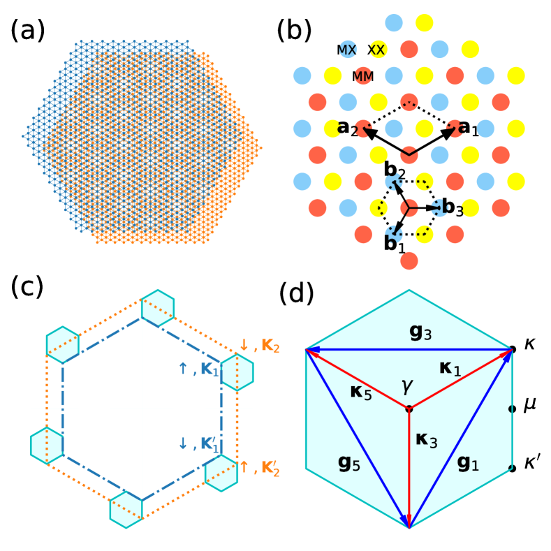
Figure 1: (a) Schematic plot (the ratio of lattice constants is not accurate) of the moiré heterobilayers. (b) The high-symmetry sites in the moiré superlattice. (c) Schematic plot of the Brillouin zone of a MoTe₂ monolayer (inside blue dash-dot hexagonal) and the Brillouin zone of a WSe₂ monolayer (inside orange dot hexagonal). The filled zone is the MBZ of AB-stacked MoTe₂/WSe₂ heterobilayers. (d) A closer look at the MBZ and high-symmetry points.

A moiré superlattice is formed due to the mismatch between the MoTe₂ hexagonal lattice and the WSe₂ hexagonal lattice with different lattice constants. Schematic plots of the moiré superlattice are illustrated in Fig. 1 (a), (b). The lattice constant of the moiré superlattice $a_{\text{M}}$ as a function of the lattice mismatch $\delta=|a^{\prime}_{0}-a_{0}|/a_{0}$ is given by $a_{\text{M}}={(1+\delta)a_{0}}/\delta$, with $a_{0}$, $a^{\prime}_{0}$ the lattice constants for the atomistic lattices. The moiré superlattice can be seen as a triangular lattice with local geometry in the unit cell. The periodicity of a triangular lattice can be studied by primitive vectors, and the local geometry can be indicated by basis vectors. The primitive vectors of the moiré superlattice can be defined as $\boldsymbol{a}_{1}=a_{\text{M}}[(\sqrt{3}/2)\mathbf{e}_{x}+(1/2)\mathbf{e}_{y}]$, $\boldsymbol{a}_{2}=a_{\text{M}}[(-\sqrt{3}/2)\mathbf{e}_{x}+(1/2)\mathbf{e}_{y}]$. The basis vectors of the moiré superlattice are given by $\boldsymbol{b}_{1}=-\left(2\boldsymbol{a}_{1}+\boldsymbol{a}_{2}\right)/3$, $\boldsymbol{b}_{2}=\left(\boldsymbol{a}_{1}+2\boldsymbol{a}_{2}\right)/3$, and $\boldsymbol{b}_{3}=\left(\boldsymbol{a}_{1}-\boldsymbol{a}_{2}\right)/3$. In Fig. 1 (b), these primitive and basis vectors are shown.

The moiré reciprocal lattice and moiré Brillouin zone (MBZ) can also be utilized to demonstrate the geometry of the moiré superlattice. The MBZ of the moiré superlattice is illustrated in Fig. 1 (c), (d). As can be seen in Fig. 1 (c), the MBZ can be constructed by the geometry difference between the Brillouin zone of a MoTe₂ monolayer and the Brillouin zone of a WSe₂ monolayer. The moiré reciprocal lattice is the periodic repeat of the Brillouin zone. For the moiré reciprocal lattice, the reciprocal primitive vectors can be defined by $\boldsymbol{g}_{i}\cdot\boldsymbol{a}_{j}=2\pi\delta_{ij}$ for $i,j=1,2$. We get $\boldsymbol{g}_{1}=\sqrt{3}k_{\text{M}}[(1/2)\mathbf{e}_{x}+(\sqrt{3}/2)\mathbf{e}_{y}]$, $\boldsymbol{g}_{2}=\sqrt{3}k_{\text{M}}[(-1/2)\mathbf{e}_{x}+(\sqrt{3}/2)\mathbf{e}_{y}]$, with $k_{\text{M}}=4\pi/(3a_{\text{M}})$. A set of reciprocal primitive vectors can be defined as

$$\boldsymbol{g}_{j}=\sqrt{3}k_{\text{M}}\left[\mathbf{e}_{x}\cos({j\pi}/{3})+\mathbf{e}_{y}\sin({j\pi}/{3})\right],$$ (1)

with $j=1,2,\cdots,6$. The high-symmetry points are indicated in Fig. 1 (d). The vector connects between $\kappa$ and $\gamma$ is given by $\boldsymbol{\kappa}_{1}=\left(2\boldsymbol{g}_{1}-\boldsymbol{g}_{2}\right)/3$ and the vector connects between $\kappa^{\prime}$ and $\gamma$ is given by $\boldsymbol{\kappa}_{2}=\left(\boldsymbol{g}_{1}-2\boldsymbol{g}_{2}\right)/3$. These two vectors $\boldsymbol{\kappa}_{1}$ and $\boldsymbol{\kappa}_{2}$ can be assigned as reciprocal basis vectors. A set of reciprocal basis vectors is defined as

$$\boldsymbol{\kappa}_{j}=k_{\text{M}}\left[\mathbf{e}_{x}\cos(\pi/6-{j\pi}/{3})+\mathbf{e}_{y}\sin(\pi/6-{j\pi}/{3})\right],$$ (2)

with $j=1,2,\cdots,6$. Part of the reciprocal primitive and basis vectors are shown in Fig. 1 (d).

II.2 Continuum model

By knowing the geometry of the moiré superlattice and the MBZ, we can write down the continuum model with effective-mass approximation. The continuum Hamiltonian for a hole in the moiré heterobilayer is written aswu2019topological ; wu2018hubbard

$$H(\mathbf{r})=\begin{pmatrix}\underline{h}_{+}(\mathbf{r})&\underline{\gamma}(\mathbf{r})\\ \underline{\gamma}^{\dagger}(\mathbf{r})&\underline{h}_{-}(\mathbf{r})\end{pmatrix},$$ (3)

with

$$\underline{h}_{\tau}(\mathbf{r})=\begin{pmatrix}h_{\tau 1}(\mathbf{r})&t_{\tau}(\mathbf{r})\\ t^{*}_{\tau}(\mathbf{r})&h_{\tau 2}(\mathbf{r})\end{pmatrix},\hskip 4.30554pt\underline{\gamma}(\mathbf{r})=\begin{pmatrix}\gamma_{1}(\mathbf{r})&0\\ 0&\gamma_{2}(\mathbf{r})\end{pmatrix},\hskip 4.30554pt$$ (4)

where $h_{\tau l}(\mathbf{r})$ is the layer Hamiltonian with $l=1,2$ indicating the top, bottom layers, $t_{\tau}(\mathbf{r})$ is the interlayer tunneling, and $\gamma_{l}(\mathbf{r})$ is the in-plane exchange field. The interlayer tunneling is given by

$$t_{\tau}(\mathbf{r})=w\left(1+e^{\mathtt{i}\tau\boldsymbol{g}_{1}\cdot\mathbf{r}}+e^{\mathtt{i}\tau\boldsymbol{g}_{2}\cdot\mathbf{r}}\right),$$ (5)

where $w$ is the interlayer-tunneling coupling. The layer Hamiltonian is given by

$$h_{\tau l}(\mathbf{r}) = \epsilon_{\tau l}+\frac{|\mathbf{p}-\tau\boldsymbol{\kappa}_{l}|^{2}}{2m_{l}}-V_{l}(\mathbf{r}),$$ (6)

where $\epsilon_{\tau l}$ is the band-edge energy and $V_{l}(\mathbf{r})$ is the moiré potential. The band-edge energy is given by

$$\epsilon_{\tau l}=[D+(-1)^{l}D]/2-(sg_{\text{spin}}+\tau g_{\text{valley}})\mu_{\text{B}}{B}_{z},$$ (7)

with $D$ the valence-band energy offset, ${B}_{z}$ the external out-of-plane magnetic field, $\mu_{\text{B}}$ the Bohr magneton, $s=+,-$ the direction for $\uparrow,\downarrow$ spin, $g_{\text{spin}}$ the spin g-factor and $g_{\text{valley}}$ the valley g-factor. Since $g_{\text{spin}}\gg g_{\text{valley}}$, accordingly, $g_{\text{valley}}\simeq{0}$ is assumed. Based on Fig. 1 (c), the spin directions of $\mathbf{K}_{l}$, $\mathbf{K}^{\prime}_{l}$ valleys at $l$-th layer are given by $s=-(-1)^{l}\tau$, with $\tau=+$ for $\mathbf{K}_{l}$ valley and $\tau=-$ for $\mathbf{K}^{\prime}_{l}$ valley. The band-edge energy can be rewritten as

$$\epsilon_{\tau 1}=-\tau M_{z},\hskip 8.61108pt\epsilon_{\tau 2}={D}+\tau M_{z}$$ (8)

with $M_{z}=g_{\text{spin}}\mu_{\text{B}}B_{z}$ an out-of-plane field-induced magnetization. The moiré potential is given by

$$V_{l}(\mathbf{r})=(-1)^{l}2V\sum_{j=1,3,5}\sin\left(\boldsymbol{g}_{j}\cdot\mathbf{r}\right)$$ (9)

where $V$ is the potential depth. For the interlayer tunneling and the moiré potential, note that $t_{\tau}(\boldsymbol{b}_{1})=t_{\tau}(\boldsymbol{b}_{2})=t_{\tau}(\boldsymbol{b}_{3})=0$ and $t_{\tau}(\mathbf{0})=t_{\tau}(\boldsymbol{a}_{1})=t_{\tau}(\boldsymbol{a}_{2})=3w$, $V_{l}(\boldsymbol{b}_{1})=V_{l}(\boldsymbol{b}_{2})=V_{l}(\boldsymbol{b}_{3})=-V_{l}(-\boldsymbol{b}_{1})=-V_{l}(-\boldsymbol{b}_{2})=-V_{l}(-\boldsymbol{b}_{3})=(-1)^{l}3\sqrt{3}V$ and $V_{l}(\mathbf{0})=V_{l}(\boldsymbol{a}_{1})=V_{l}(\boldsymbol{a}_{2})=0$. These points can be assigned at the high-symmetry sites in the moiré superlattice. If the coordinate is transformed as $\mathbf{r}\rightarrow\mathbf{r}+\boldsymbol{b}_{2}$, the moiré potential and the interlayer tunneling become

$$V_{l}(\mathbf{r}+\boldsymbol{b}_{2}) = (-1)^{l}2V\sum_{j=1,3,5}\cos\left(\boldsymbol{g}_{j}\cdot\mathbf{r}+{\pi}/{6}\right),$$ (10)

$$t_{\tau}(\mathbf{r}+\boldsymbol{b}_{2}) = w\left[1+e^{\mathtt{i}\tau\left(\boldsymbol{g}_{1}\cdot\mathbf{r}+{2\pi}/{3}\right)}+e^{\mathtt{i}\tau\left(\boldsymbol{g}_{2}\cdot\mathbf{r}+{4\pi}/{3}\right)}\right].\hskip 12.91663pt$$ (11)

The later formulation of moiré potential and interlayer tunneling is more frequently seen in literature, but the two formulations are equivalent.

The in-plane exchange field includes the contributions from a ferromagnetic exchange field and a $120^{\circ}$-antiferromagnetic exchange field, which are generated from an in-plane ferromagnetic order and an in-plane $120^{\circ}$-Néel order, respectively. The origins of these two magnetic orders will be discussed in Sec. III and Sec. IV. Note that the in-plane exchange field is not uniformly effective, since the magnetic order is originated from localized spins residing at each moiré unit cell. The exchange field should show the same periodicity as the moiré superlattice. The $120^{\circ}$-Néel order is a three-sublattice antiferromagnetic order with the directions of spins at three sublattices being separated by $2\pi/3$ angular differenceleung1993spin ; wu2018hubbard ; pan2020band ; zang2021hartree . A general form of the three-sublattice exchange field is written as

$$\gamma_{l}(\mathbf{r}) = e^{\mathtt{i}2\boldsymbol{\kappa}_{l}\cdot\mathbf{r}}\big{[}M_{A}\exp\left(\mathtt{i}\boldsymbol{\kappa}_{1}\cdot(\mathbf{r}-\boldsymbol{b}_{1})\right)$$ (12)

$$+M_{B}\exp\left(\mathtt{i}\boldsymbol{\kappa}_{3}\cdot(\mathbf{r}-\boldsymbol{b}_{2})\right)$$

$$+M_{C}\exp\left(\mathtt{i}\boldsymbol{\kappa}_{5}\cdot(\mathbf{r}-\boldsymbol{b}_{3})\right)\big{]},$$

where $M_{A}$, $M_{B}$, $M_{C}$ are sublattice magnetizations. The phase term $e^{\mathtt{i}2\boldsymbol{\kappa}_{l}\cdot\mathbf{r}}$ is added to the exchange field to counter the phase difference between single-particle states at two valleys. For the in-plane ferromagnetic order, sublattice magnetizations follow the relation $M_{A}=M_{B}=M_{C}$. The in-plane ferromagnetic exchange field is then given by

$$\gamma_{l}(\mathbf{r}) = e^{\mathtt{i}2\boldsymbol{\kappa}_{l}\cdot\mathbf{r}}M_{\perp}\sum_{j=1,3,5}\exp\left(\mathtt{i}\boldsymbol{\kappa}_{j}\cdot\mathbf{r}\right),$$ (13)

with $M_{\perp}$ the in-plane ferromagnetic magnetization. On the other hand, for the in-plane $120^{\circ}$-Néel order, sublattice magnetizations follow the relation $M_{A}=\exp(\mathtt{i}2\pi/3)M_{B}=\exp(\mathtt{i}4\pi/3)M_{C}$. The in-plane $120^{\circ}$-antiferromagnetic exchange field is given by

$$\gamma_{l}(\mathbf{r}) = e^{\mathtt{i}2\boldsymbol{\kappa}_{l}\cdot\mathbf{r}}M^{\prime}_{\perp}\big{[}\exp\left(\mathtt{i}(\boldsymbol{\kappa}_{1}\cdot\mathbf{r}+4\pi/3)\right)$$ (14)

$$+\exp\left(\mathtt{i}(\boldsymbol{\kappa}_{3}\cdot\mathbf{r}+2\pi/3)\right)+\exp\left(\mathtt{i}\boldsymbol{\kappa}_{5}\cdot\mathbf{r}\right)\big{]},$$

with $M^{\prime}_{\perp}$ the in-plane antiferromagnetic magnetization.

II.3 Symmetry

The TRS and three-fold rotational ($C_{3}$) symmetry of the continuum model are discussed. The time-reversal operation ($\Theta$) is defined by $\Theta=\exp\left(-\mathtt{i}\pi\sigma_{y}/2\right)\mathcal{K}=-\mathtt{i}\sigma_{y}\mathcal{K}$, where $\mathcal{K}$ is defined by

$$\mathcal{K}\mathtt{i}\mathcal{K}^{-1}=-\mathtt{i},\hskip 8.61108pt\mathcal{K}\mathbf{p}\mathcal{K}^{-1}=-\mathbf{p}.$$ (15)

The $-\mathtt{i}\sigma_{y}$ operation gives $-\mathtt{i}\sigma_{y}|+\rangle=|-\rangle$ and $-\mathtt{i}\sigma_{y}|-\rangle=-|+\rangle$, where $|+\rangle$ and $|-\rangle$ are the state kets with valley numbers $\tau=+,-$. It can be found that $\Theta|\tau\rangle\left[h_{\tau l}(\mathbf{r})-\epsilon_{\tau l}\right]\langle\tau|\Theta^{-1}=|-\tau\rangle\left[h_{-\tau l}(\mathbf{r})-\epsilon_{-\tau l}\right]\langle-\tau|$, and $\Theta|\tau\rangle{t}_{\tau}(\mathbf{r})\langle\tau|\Theta^{-1}=|-\tau\rangle{t}_{-\tau}(\mathbf{r})\langle-\tau|$. For the out-of-plane magnetic field, the time-reversal operation gives $\Theta|\tau\rangle\epsilon_{\tau l}\langle\tau|\Theta^{-1}=|-\tau\rangle\epsilon_{\tau l}\langle-\tau|$. For the in-plane exchange field, the time-reversal operation gives $\Theta|+\rangle{\gamma}_{l}(\mathbf{r})\langle-|\Theta^{-1}=-|-\rangle{\gamma}^{*}_{l}(\mathbf{r})\langle+|$ and $\Theta|-\rangle{\gamma}^{*}_{l}(\mathbf{r})\langle+|\Theta^{-1}=-|+\rangle{\gamma}_{l}(\mathbf{r})\langle-|$. Therefore, the continuum Hamiltonian in the absence of a magnetic field and exchange field is invariant under the time-reversal operation, and the directions of magnetizations are reversed $(M_{z},M_{\perp},M^{\prime}_{\perp})\rightarrow(-M_{z},-M_{\perp},-M^{\prime}_{\perp})$ in the Hamiltonian with out-of-plane magnetic fields and in-plane exchange fields. Therefore, the magnetizations $M_{z},M_{\perp},M^{\prime}_{\perp}$ can be considered as TRS breaking terms.

To study the $C_{3}$ symmetry of the continuum model, it is convenient to apply a unitary transformation to the Hamiltonian $\bar{H}(\mathbf{r})=\mathcal{U}(\mathbf{r}){H}(\mathbf{r})\mathcal{U}^{\dagger}(\mathbf{r})$, where the unitary transformation matrix is given by

$$\mathcal{U}(\mathbf{r}) = \begin{pmatrix}e^{-\mathtt{i}\boldsymbol{\kappa}_{1}\cdot\mathbf{r}}&0&0&0\\ 0&e^{-\mathtt{i}\boldsymbol{\kappa}_{2}\cdot\mathbf{r}}&0&0\\ 0&0&e^{\mathtt{i}\boldsymbol{\kappa}_{1}\cdot\mathbf{r}}&0\\ 0&0&0&e^{\mathtt{i}\boldsymbol{\kappa}_{2}\cdot\mathbf{r}}\end{pmatrix},$$ (16)

with the basis $(\tau,l)=(+,1),(+,2),(-,1),(-,2)$. The layer Hamiltonian becomes

$$\bar{h}_{\tau l}(\mathbf{r}) = \epsilon_{\tau l}+\frac{|\mathbf{p}|^{2}}{2m_{l}}-V_{l}(\mathbf{r}),$$ (17)

and the interlayer tunneling becomes

$$\bar{t}_{\tau}(\mathbf{r})=w\sum_{j=1,3,5}\exp\left({\mathtt{i}\tau\boldsymbol{\kappa}_{j}\cdot\mathbf{r}}\right).$$ (18)

The in-plane exchange field including both ferromagnetic magnetization and antiferromagnetic magnetization is given by

$$\bar{\gamma}_{l}(\mathbf{r}) = M_{\perp}\sum_{j=1,3,5}\exp\left(\mathtt{i}\boldsymbol{\kappa}_{j}\cdot\mathbf{r}\right)$$ (19)

$$+M^{\prime}_{\perp}\sum_{j=1,3,5}\big{[}\exp\left(\mathtt{i}(\boldsymbol{\kappa}_{1}\cdot\mathbf{r}+4\pi/3)\right)$$

$$+\exp\left(\mathtt{i}(\boldsymbol{\kappa}_{3}\cdot\mathbf{r}+2\pi/3)\right)+\exp\left(\mathtt{i}\boldsymbol{\kappa}_{5}\cdot\mathbf{r}\right)\big{]}.$$

The $C_{3}$ operation is defined by

$$C_{3}\bar{H}(\mathbf{r})C_{3}^{-1}=\bar{H}(\mathbb{R}_{[-2\pi/3]}\mathbf{r}),$$ (20)

where the rotational matrix satisfies

$$\mathbb{R}_{[\theta]}\boldsymbol{v}=\begin{pmatrix}\cos\theta&\sin\theta\\ -\sin\theta&\cos\theta\end{pmatrix}\begin{pmatrix}v_{x}\\ v_{y}\end{pmatrix}$$ (21)

for arbitrary vector $\boldsymbol{v}$. The rotational matrix gives $\mathbb{R}_{[4\pi/3]}\boldsymbol{g}_{1}=\mathbb{R}_{[2\pi/3]}\boldsymbol{g}_{3}=\boldsymbol{g}_{5}$, and $\mathbb{R}_{[4\pi/3]}\boldsymbol{\kappa}_{5}=\mathbb{R}_{[2\pi/3]}\boldsymbol{\kappa}_{3}=\boldsymbol{\kappa}_{1}$. It is found that the $C_{3}$-symmetry is conserved for the continuum model with the ferromagnetic exchange field. On the other hand, the in-plane antiferromagnetic exchange field breaks the $C_{3}$ symmetry.

II.4 Moiré band structure

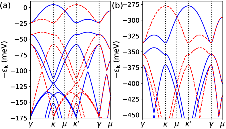
Figure 2: Moiré band structures of holes contributed from (a) the MoTe₂ layer and (b) the WSe₂ layer of a AB-stacked heterobilayer simulated by the continuum model and the plane-wave method in the absence of interlayer tunneling and magnetization. The blue solid line indicates $\tau=+$ and the red dash line indicates $\tau=-$. The high symmetry points are tagged in the MBZ in Fig. 1 (d).

The effective hole mass of the MoTe₂ is given by $m_{1}/m_{0}=0.62$ and the effective hole mass of the WSe₂ is $m_{2}/m_{0}=0.36$xiao2012coupled ; kylanpaa2015binding . The parameters for the moiré heterobilayers are assumed to be $D=280$ meV, $V=10$ meV, $a_{\text{M}}=50$ Å, and $w=1.0$ meV. The interlayer-tunneling coupling is small because the interlayer tunneling is spin-forbidden in the leading order approximation for the moiré heterobilayersexp0 ; theory2 . The single-particle band structure of the moiré superlattice, name as moiré band structure, can be calculated by using the plane-wave basis function method (see appendix Sec. A.1). While the interlayer-tunneling coupling is small in comparing with the valence-band offset, the moiré band structure is studied in the absence of the interlayer tunneling, such that the moiré bands can be assigned as contributions from different layers. In Fig. 2, moiré band structures for holes contributed from the MoTe₂ layer and the WSe₂ layer of the moiré heterobilayers in the absence of interlayer tunneling and magnetization are shown. Note that an intrinsic band inversion locates across $\gamma-\mu$ lines in the MBZ between the highest two moiré hole bands with opposite valley numbers in the MoTe₂ layer. In Sec. III, we will study how Coulomb interaction opens a gap at the intrinsically inverted moiré bands and how the topological order emerges.

III interaction-driven Chern band

In this section, the formation of the Chern band in the QAH state is studied. The Chern band is generated by opening a gap to break the intrinsic band inversion across $\gamma-\mu$ lines. The gap is opened by in-plane exchange fields contributed from corresponding Coulomb-interaction-driven in-plane $120^{\circ}$-Néel order and in-plane ferromagnetic order. The Néel order ensures the insulating gap and the ferromagnetic order generates the non-zero Chern number. In Sec. III.1, the many-particle Hamiltonian for Coulomb-interacting systems and Hartree-Fock approximation are introduced. The method to calculate Chern numbers for single-particle band structures in interacting systems is reviewed. In Sec. III.2, the $120^{\circ}$-Néel order is derived from the Hartree-Fock exchange interaction. The competition between the $120^{\circ}$-Néel order and the valley polarization of holes driven by an external magnetic field is studied. Effects of the Néel order and the ferromagnetic order on the gap opening are discussed. In Sec. III.3, Chern numbers of moiré bands are assigned by studying the winding numbers of Fock pseudospin textures.

III.1 Interacting systems

To include the Coulomb interaction in the band-structure picture, we consider the many-particle Hamiltonian for multi-component fermion fields

$$\hat{\mathcal{H}} = \sum_{ab}\int\hat{\Psi}^{\dagger}_{a}(\mathbf{r})H_{ab}(\mathbf{r})\hat{\Psi}_{b}(\mathbf{r})\text{d}^{2}r$$ (22)

$$+\frac{1}{2}\sum_{ab}\int W_{ab}(\mathbf{r}_{12}):\hat{\rho}_{a}(\mathbf{r}_{1})\hat{\rho}_{b}(\mathbf{r}_{2}):\text{d}^{2}r_{1}\text{d}^{2}r_{2},$$

where $a=\{\tau,l\}$ is the component index. $H_{ab}(\mathbf{r})$ is the continuum Hamiltonian given in Eq. (3), $W_{ab}(\mathbf{r}_{12})$ is the Coulomb potential, $\hat{\Psi}^{\dagger}_{a}(\mathbf{r})$ and $\hat{\Psi}_{a}(\mathbf{r})$ are fermion creation and annihilation operators for charges, and $\hat{\rho}_{a}(\mathbf{r})=\hat{\Psi}^{\dagger}_{a}(\mathbf{r})\hat{\Psi}_{a}(\mathbf{r})$ is the density operator. The Chern number $\mathcal{C}$ of an insulator can be related to the quantized Hall conductance by $\sigma_{\text{H}}=\frac{e^{2}}{2\pi}\mathcal{C}$. For interacting many-particle systems, the Chern number contributed from the band structures can be calculated byhohenadler2013correlation ; so1985induced ; ishikawa1987microscopic ; matsuyama1987quantization ; wang2010topological

$$\mathcal{C} = \frac{\epsilon_{\mu\nu\rho}}{6}\int\text{Tr}\left[\tilde{\mathcal{G}}\frac{\partial{\tilde{\mathcal{G}}}^{-1}}{\partial k_{\mu}}\tilde{\mathcal{G}}\frac{\partial{\tilde{\mathcal{G}}}^{-1}}{\partial k_{\nu}}\tilde{\mathcal{G}}\frac{\partial{\tilde{\mathcal{G}}}^{-1}}{\partial k_{\rho}}\right]\frac{\text{d}^{3}k}{(2\pi)^{2}},$$ (23)

where $\tilde{\mathcal{G}}(k)=\int e^{\mathtt{i}k\cdot{r}}\mathcal{G}(r)\text{d}^{3}r$ is the Matsubara single-particle Green’s function, with $k=(\mathtt{i}\omega,k_{x},k_{y})$, $r=(-\mathtt{i}\bar{t},x,y)$, $\bar{t}$ the proper time variable, $\mu,\nu,\rho\in\{0,1,2\}$ the coordinate indices, and $\epsilon_{\mu\nu\rho}$ being the Levi-Civita symbol. Note that the Einstein summation convention has been applied. The single-particle Green’s function is defined as $\mathcal{G}_{ab}(r-r^{\prime})\equiv-\langle{\hat{\mathcal{T}}\big{[}\hat{\Psi}_{a}(r)\hat{\Psi}^{\dagger}_{b}(r^{\prime})\big{]}}\rangle$, with $\hat{\mathcal{T}}$ the time-ordering operator. The Fourier transform of the Green’s function $\tilde{\mathcal{G}}(k)=\tilde{\mathcal{G}}_{\mathbf{k}}(\mathtt{i}\omega)$ can be solved by $\tilde{\mathcal{G}}_{\mathbf{k}}(\mathtt{i}\omega)=\big{[}\mathtt{i}\omega-\tilde{H}_{\mathbf{k}}-\tilde{\Sigma}_{\mathbf{k}}(\mathtt{i}\omega)\big{]}^{-1}$, where the self-energy $\tilde{\Sigma}_{\mathbf{k}}(\mathtt{i}\omega)$ includes the effect of interactions.

Hartree-Fock approximation can be used to find the band structure and solve the single-particle Green’s function of interacting systems. The field creation and annihilation operators can be transformed as $\hat{\Psi}_{a}(\mathbf{r})=\sum_{n\mathbf{k}}\psi_{a,n\mathbf{k}}(\mathbf{r})\hat{d}_{n\mathbf{k}}$ and $\hat{\Psi}^{\dagger}_{a}(\mathbf{r})=\sum_{n\mathbf{k}}\psi^{*}_{a,n\mathbf{k}}(\mathbf{r})\hat{d}^{\dagger}_{n\mathbf{k}}$, where $\psi_{a,n\mathbf{k}}(\mathbf{r})$ is the hole wavefunction and $\hat{d}^{\dagger}_{n\mathbf{k}}$/$\hat{d}_{n\mathbf{k}}$ is hole creation/annihilation operator with band index $n$ and momentum $\mathbf{k}$. The Hartree-Fock variational ground state for the hole-filled insulator is assumed to be $|{\text{HF}}\rangle=\prod_{n\mathbf{k}}\hat{d}^{\dagger}_{n\mathbf{k}}|{0}\rangle$, with the vacuum state $|{0}\rangle$ being fully-occupied valence bands (empty hole bands). A plane-wave basis function method $\psi_{a,n\mathbf{k}}(\mathbf{r})=\sum_{\mathbf{G}}u_{(a,\mathbf{G}),n\mathbf{k}}\phi_{\mathbf{G},\mathbf{k}}(\mathbf{r})$ can be used to find the single-particle wavefunction under Hartree-Fock approximation, where the wavefunction coefficient $u_{(a,\mathbf{G}),n\mathbf{k}}$ is solved from a Hartree-Fock equation $\tilde{F}_{\mathbf{k}}u_{n\mathbf{k}}=\varepsilon_{n\mathbf{k}}u_{n\mathbf{k}}$, with $\tilde{F}_{\mathbf{k}}$ being the Fock matrix (see Appendix A.1 and A.2). To study the effect of Coulomb interaction on band topology, the band structure can be calculated by Hartree-Fock approximation and the Chern number can be found by solving Eq. (23) with the self-energy $\tilde{\Sigma}_{\mathbf{k}}(\mathtt{i}\omega)=\tilde{F}_{\mathbf{k}}-\tilde{H}_{\mathbf{k}}$. Under this scheme, the Fock matrix can be viewed as an effective single-particle Hamiltonian.

III.2 Néel order and gap opening

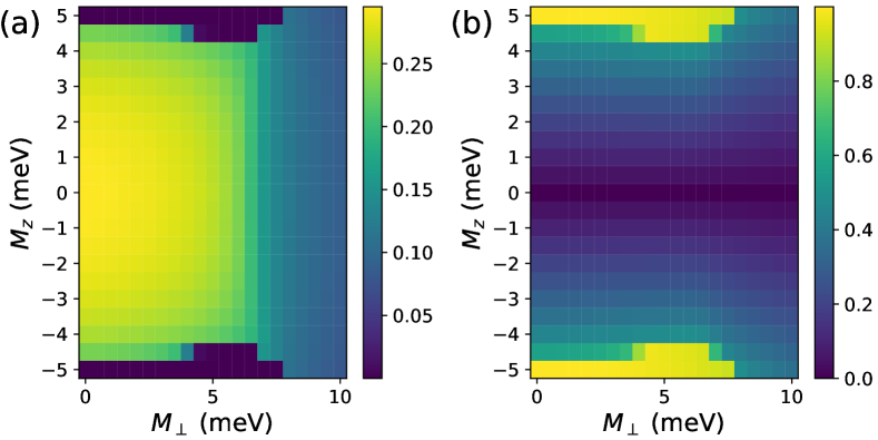
Figure 3: Color plots of (a) the $120^{\circ}$-Néel order parameter $\eta^{\prime}$ and (b) the degree of valley polarization $\delta=|n_{+}-n_{-}|/(n_{+}+n_{-})$ as the functions of in-plane ferromagnetic magnetization $M_{\perp}$ and out-of-plane field-induced magnetization $M_{z}$ simulated by Hartree-Fock approximation of the six-band model with contact potential.

Since the interlayer-tunneling coupling is much smaller than the valence-band energy offset and the holes largely reside at the MoTe₂ layer, only the moiré band structure of the MoTe₂ layer is considered in this section. The band structure is obtained by solving the eigenvalue problem $\tilde{F}_{\mathbf{k}}u_{n\mathbf{k}}=\varepsilon_{n\mathbf{k}}u_{n\mathbf{k}}$. The Fock matrix is given by $\tilde{F}_{\mathbf{k}}=\tilde{H}_{\mathbf{k}}+\tilde{K}_{\mathbf{k}}-\tilde{J}_{\mathbf{k}}$, where $\tilde{H}_{\mathbf{k}}$ is the Bloch Hamiltonian, $\tilde{K}_{\mathbf{k}}$ is the Coulomb-integral matrix and $\tilde{J}_{\mathbf{k}}$ is the exchange-integral matrix (see Appendix A.2). The Bloch Hamiltonian in the plane-wave basis reads $\langle\tau_{1},\mathbf{G}_{1}|\tilde{H}_{\mathbf{k}}|\tau_{2},\mathbf{G}_{2}\rangle=\int\phi^{*}_{\mathbf{G}_{1},\mathbf{k}}(\mathbf{r})H_{\tau_{1}\tau_{2}}(\mathbf{r})\phi_{\mathbf{G}_{2},\mathbf{k}}(\mathbf{r})\text{d}^{2}r$ with $\phi_{\mathbf{G},\mathbf{k}}(\mathbf{r})=e^{\mathtt{i}\left(\mathbf{k}-\mathbf{G}\right)\cdot\mathbf{r}}/\sqrt{S}$, where ${S}=({\sqrt{3}}/{2})Na^{2}_{\text{M}}$ is the area of the moiré lattice with $N$ the number of moiré unit cell. Considering that the continuum model for the MoTe₂ monolayer is expanded by six plane-wave basis functions, $|\tau,\mathbf{0}\rangle$, $|\tau,-\tau\boldsymbol{g}_{1}\rangle$, $|\tau,\tau\boldsymbol{g}_{3}\rangle$ with $\tau=\pm$, which can also be written as $|\tau,\tau\boldsymbol{\kappa}_{J}-\tau\boldsymbol{\kappa}_{1}\rangle$ with $J=1,3,5$ and $\tau=\pm$, a six-band model can be derived. The Hamiltonian matrix of the six-band model is written as

$$\tilde{H}_{\mathbf{k}}=\begin{pmatrix}\tilde{h}_{\mathbf{k}}-M_{z}\mathbb{I}&\tilde{\gamma}_{\mathbf{k}}\\ \tilde{\gamma}^{*}_{\mathbf{k}}&\tilde{h}^{*}_{-\mathbf{k}}+M_{z}\mathbb{I}\end{pmatrix},$$ (24)

where $\mathbb{I}$ is a three-by-three identity matrix, $\tilde{h}_{\mathbf{k}}$ is the valley-subspace Hamiltonian matrix, and $\tilde{\gamma}_{\mathbf{k}}$ is the in-plane exchange-field matrix. The valley-subspace Hamiltonian matrix is given by

$$\tilde{h}_{\mathbf{k}}=\begin{pmatrix}\frac{|\mathbf{k}-\boldsymbol{\kappa}_{1}|^{2}}{2m_{1}}&-\mathtt{i}V&\mathtt{i}V\\ \mathtt{i}V&\frac{|\mathbf{k}-\boldsymbol{\kappa}_{3}|^{2}}{2m_{1}}&-\mathtt{i}V\\ -\mathtt{i}V&\mathtt{i}V&\frac{|\mathbf{k}-\boldsymbol{\kappa}_{5}|^{2}}{2m_{1}}\end{pmatrix}.$$ (25)

The in-plane exchange-field matrix is written as

$$\tilde{\gamma}_{\mathbf{k}}=M_{\perp}\begin{pmatrix}0&1&1\\ 1&0&1\\ 1&1&0\end{pmatrix}+M^{\prime}_{\perp}\begin{pmatrix}0&1&e^{\mathtt{i}2\pi/3}\\ 1&0&e^{\mathtt{i}4\pi/3}\\ e^{\mathtt{i}2\pi/3}&e^{\mathtt{i}4\pi/3}&0\end{pmatrix},$$

where $M^{\prime}_{\perp}=0$ is assigned since the antiferromagnetic magnetization should be contributed from the Hartree-Fock exchange interaction. The Coulomb potential in Eq. (22) is approximated by a contact potential $W_{ab}(\mathbf{r})\simeq(S/N)U\delta(\mathbf{r})$, with $U$ the contact-potential energy. The Coulomb-integral matrix is given by $\langle\tau,\tau\boldsymbol{\kappa}_{I}-\tau\boldsymbol{\kappa}_{1}|\tilde{K}_{\mathbf{k}}|\tau,\tau\boldsymbol{\kappa}_{J}-\tau\boldsymbol{\kappa}_{1}\rangle=U\sum_{\tau^{\prime}}\langle\boldsymbol{\kappa}_{I}|\rho_{\tau^{\prime}\tau^{\prime}}|\boldsymbol{\kappa}_{J}\rangle$ and the exchange-integral matrix is given by $\langle\tau,\tau\boldsymbol{\kappa}_{I}-\tau\boldsymbol{\kappa}_{1}|\tilde{J}_{\mathbf{k}}|\tau^{\prime},\tau^{\prime}\boldsymbol{\kappa}_{J}-\tau^{\prime}\boldsymbol{\kappa}_{1}\rangle=U\langle\boldsymbol{\kappa}_{I}|\rho_{\tau\tau^{\prime}}|\boldsymbol{\kappa}_{J}\rangle$, where

$$\langle\boldsymbol{\kappa}_{I}|\rho_{\tau\tau^{\prime}}|\boldsymbol{\kappa}_{J}\rangle \equiv \frac{1}{N}\sum_{\mathbf{k},\mathbf{G},n}\tilde{n}_{n\mathbf{k}}{u}_{(\tau,\mathbf{G}+\tau\boldsymbol{\kappa}_{I}-\tau\boldsymbol{\kappa}_{1}),n\mathbf{k}}$$ (27)

$$\times{u}^{*}_{(\tau^{\prime},\mathbf{G}+\tau^{\prime}\boldsymbol{\kappa}_{J}-\tau^{\prime}\boldsymbol{\kappa}_{1}),n\mathbf{k}},$$

is the single-particle density matrix. The Fock matrix can be written as

$$\tilde{F}_{\mathbf{k}}=\begin{pmatrix}\tilde{h}_{\mathbf{k}}+U\rho_{--}-M_{z}\mathbb{I}&\tilde{\gamma}_{\mathbf{k}}-U\rho_{+-}\\ \tilde{\gamma}^{*}_{\mathbf{k}}-U\rho_{-+}&\tilde{h}^{*}_{-\mathbf{k}}+U\rho_{++}+M_{z}\mathbb{I}\end{pmatrix},$$ (28)

with

$$\rho_{\tau\tau}=\begin{pmatrix}n_{\tau}&\varrho_{\tau}&\varrho^{*}_{\tau}\\ \varrho^{*}_{\tau}&n_{\tau}&\varrho_{\tau}\\ \varrho_{\tau}&\varrho^{*}_{\tau}&n_{\tau}\end{pmatrix},\hskip 4.30554pt\rho_{+-}=\begin{pmatrix}\xi_{1}&\eta_{5}&\eta_{3}\\ \eta_{5}&\xi_{3}&\eta_{1}\\ \eta_{3}&\eta_{1}&\xi_{5}\end{pmatrix},$$ (29)

and $\rho_{-+}=\rho_{+-}^{*}$. Matrix elements of the single-particle density matrix are given by $n_{\tau}=\langle\boldsymbol{\kappa}_{I}|\rho_{\tau\tau}|\boldsymbol{\kappa}_{I}\rangle$, $\xi_{I}=\langle\boldsymbol{\kappa}_{I}|\rho_{+-}|\boldsymbol{\kappa}_{I}\rangle$ with $I=1,3,5$, and $\varrho_{\tau}=\langle\boldsymbol{\kappa}_{1}|\rho_{\tau\tau}|\boldsymbol{\kappa}_{3}\rangle$, $\eta_{1}=\langle\boldsymbol{\kappa}_{5}|\rho_{+-}|\boldsymbol{\kappa}_{3}\rangle$, $\eta_{3}=\langle\boldsymbol{\kappa}_{1}|\rho_{+-}|\boldsymbol{\kappa}_{5}\rangle$, $\eta_{5}=\langle\boldsymbol{\kappa}_{3}|\rho_{+-}|\boldsymbol{\kappa}_{1}\rangle$. If a $120^{\circ}$-Néel order emerges, the exchange interaction $-U\rho_{-+}$ can be treated as an antiferromagnetic exchange field, and the density matrix should be described by the forms $\eta_{1}=\eta+e^{\mathtt{i}4\pi/3}\eta^{\prime}$, $\eta_{3}=\eta+e^{\mathtt{i}2\pi/3}\eta^{\prime}$, $\eta_{5}=\eta+\eta^{\prime}$, with $\eta$ and $\eta^{\prime}$ being order parameters to quantify the ferromagnetic order and $120^{\circ}$-Néel order respectively. The Hartree-Fock equation can be solved iteratively. By using the form of the density matrix as the initial guess for the iteration of the Hartree-Fock calculation, converged solutions of the density matrix and band structure can be obtained. A gap opening in the moiré band structure can be found after the iteration. It implies that Coulomb interaction induces a $120^{\circ}$-Néel order by breaking the lattice translational symmetry and contributes to an antiferromagnetic exchange field.

A valley polarization of holes in the Hartree-Fock ground state can be induced by applying an out-of-plane external magnetic field to the system. A degree of valley polarization for hole doping is defined as $\delta=|n_{+}-n_{-}|/(n_{+}+n_{-})$. In Fig. 3, color plots of the $120^{\circ}$-Néel order parameter $\eta^{\prime}$ and the degree of valley polarization $\delta$ as the functions of in-plane ferromagnetic magnetization $M_{\perp}$ and out-of-plane magnetization $M_{z}$ are shown. It is found that the $120^{\circ}$-Néel order and the field-induced valley polarization compete with each other. For a wide range of magnetizations, the Néel order and the valley polarization also coexist. The coexistence implies that a canted spin texture could exist in the moiré superlattice. Additionally, as can be seen in Fig. 3 (a), the $120^{\circ}$-Néel order is suppressed by the ferromagnetic magnetization but is not vanishing. It implies the coexistence of the in-plane $120^{\circ}$-Néel order and the in-plane ferromagnetic order. As will be shown later in Sec. III.3, the second coexistence is crucial to the formation of the Chern band.

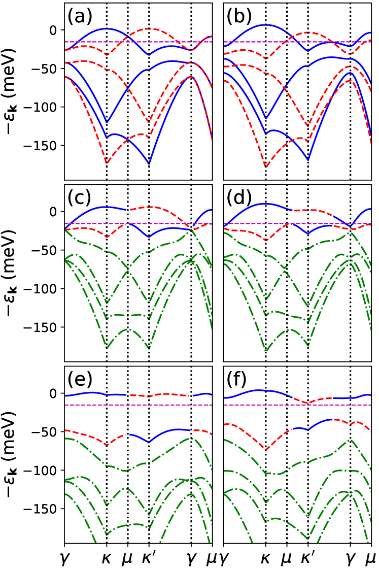
Figure 4: Moiré band structures contributed from the MoTe₂ layer simulated by Hartree-Fock approximation of the six-band model with contact potential. The parameters by the unit of meV are (a) $M_{\perp}=0$, $M_{z}=0$, $U=0$; (b) $M_{\perp}=0$, $M_{z}=5$, $U=0$; (c) $M_{\perp}=10$, $M_{z}=0$, $U=0$; (d) $M_{\perp}=10$, $M_{z}=5$, $U=0$; (e) $M_{\perp}=10$, $M_{z}=0$, $U=70$; (f) $M_{\perp}=10$, $M_{z}=5$, $U=70$. The horizontal dashed lines indicate the Fermi level at $\nu$=1 filling.

Moiré band structures simulated by the six-band model in the absence of Coulomb interaction with and without the in-plane ferromagnetic exchange field are shown in Fig. 4 (a), (b), (c), and (d). It is found that, in the absence of the in-plane ferromagnetic and antiferromagnetic exchange fields, the highest two moiré bands with opposite valley numbers intersect with each other. Additionally, as shown in Fig. 4 (b), the crossing over between two moiré bands, which can be seen as a band inversion, survives with a small out-of-plane magnetic field. The horizontal dashed line indicates the Fermi level at $\nu$=1 filling. Since the Fermi level crosses the moiré bands, holes occupying these bands would form a Fermi sea and show a metallic transport property. In Fig. 4 (c) and (d), it is found that the in-plane ferromagnetic exchange field opens a gap at the band inversion along the line $\gamma-\mu$ in the MBZ. However, the gap is not entirely opened at the high symmetry point $\gamma$ and the Fermi level is still crossing the moiré bands. In Fig. 4 (e) and (f), moiré band structures solved from Hartree-Fock approximation of the six-band model with contact potential are shown. A gap is opened along the crossing line between the two highest bands. The gap is opened by the antiferromagnetic exchange field induced by the $120^{\circ}$-Néel order. The hole-occupied band, the highest band in Fig. 4 (f), has a valley-polarized population of holes majorly with $\tau=+$. Because of the gap, the $120^{\circ}$-Néel order and the field-induced valley polarization can coexist. Since the Fermi level resides between the highest two moiré bands, the holes only occupy the highest moiré band and show an insulating transport property. It indicates that the $120^{\circ}$-Néel order ensures the insulating gap.

III.3 Chern number

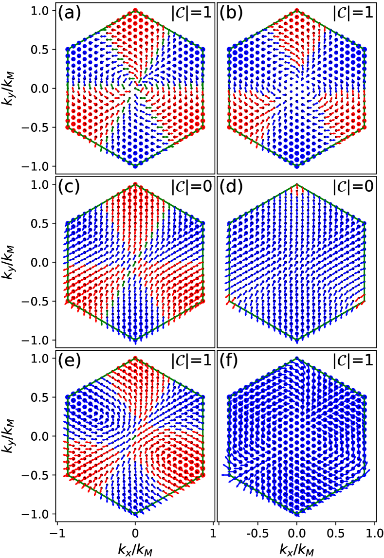
Figure 5: Fock pseudospin textures in the MBZ contributed from the MoTe₂ layer simulated by Hartree-Fock approximation of the six-band model with contact potential. The parameters by the unit of meV are (a) $M_{\perp}=5$, $M_{z}=0$, $U=0$; (b) $M_{\perp}=5$, $M_{z}=3$, $U=0$; (c) $M_{\perp}=5$, $M_{z}=0$, $U=70$; (d) $M_{\perp}=5$, $M_{z}=3$, $U=70$; (e) $M_{\perp}=10$, $M_{z}=0$, $U=70$; (f) $M_{\perp}=5$, $M_{z}=5$, $U=70$.

In this section, the Chern numbers of moiré bands simulated by Hartree-Fock approximation of the six-band model with contact potential are studied. To demonstrate the emergence of the topological order, the Fock matrix is reduced to a two-by-two matrix by a projection transformation as

$$\tilde{\mathcal{F}}_{\mathbf{k}}=\mathcal{P}^{\dagger}_{\mathbf{k}}\tilde{F}_{\mathbf{k}}\mathcal{P}_{\mathbf{k}}=\begin{pmatrix}\varepsilon_{+,\mathbf{k}}-M_{z}&f_{+-,\mathbf{k}}\\ f_{-+,\mathbf{k}}&\varepsilon_{-,\mathbf{k}}+M_{z}\end{pmatrix},$$ (30)

where $\mathcal{P}_{\mathbf{k}}=\begin{pmatrix}\mathcal{P}_{+,\mathbf{k}}&0\\ 0&\mathcal{P}_{-,\mathbf{k}}\end{pmatrix}$ is the projection matrix with $\mathcal{P}_{\pm,\mathbf{k}}$ following the unitary condition $\mathcal{P}^{\dagger}_{\pm,\mathbf{k}}\mathcal{P}_{\pm,\mathbf{k}}=1$, and $\varepsilon_{\pm,\mathbf{k}}$ is solved from the eigenvalue equation $\big{(}\tilde{h}_{\mathbf{k}}+U\rho_{\mp\mp}\big{)}\mathcal{P}_{\pm,\mathbf{k}}=\varepsilon_{\pm,\mathbf{k}}\mathcal{P}_{\pm,\mathbf{k}}$ as the lowest eigenvalue. The off-diagonal matrix elements are given by $f_{-+,\mathbf{k}}=\mathcal{P}^{\dagger}_{-,\mathbf{k}}\big{(}\tilde{\gamma}^{*}_{\mathbf{k}}-U\rho_{-+}\big{)}\mathcal{P}_{+,\mathbf{k}}$, $f_{+-,\mathbf{k}}=\mathcal{P}^{\dagger}_{-,\mathbf{k}}\big{(}\tilde{\gamma}_{\mathbf{k}}-U\rho_{+-}\big{)}\mathcal{P}_{+,\mathbf{k}}$. The reduced Fock matrix can be reformulated by the parametrized Fock pseudospin $\tilde{\mathcal{F}}_{\mathbf{k}}=\tilde{\mathcal{F}}_{\mathbf{k},0}\mathbb{I}+\tilde{\mathcal{F}}_{\mathbf{k},x}\sigma_{x}+\tilde{\mathcal{F}}_{\mathbf{k},y}\sigma_{y}+\tilde{\mathcal{F}}_{\mathbf{k},z}\sigma_{z}$. Based on Eq. (23) and the argument in Sec. III.1, the Chern number can be calculated bybernevig2013topological

$$\mathcal{C}=\frac{1}{4\pi}\int_{\text{BZ}}\frac{\tilde{\boldsymbol{\mathcal{F}}}_{\mathbf{k}}\cdot\partial_{k_{x}}\tilde{\boldsymbol{\mathcal{F}}}_{\mathbf{k}}\times\partial_{k_{y}}\tilde{\boldsymbol{\mathcal{F}}}_{\mathbf{k}}}{|\tilde{\boldsymbol{\mathcal{F}}}_{\mathbf{k}}|^{3}}\text{d}^{2}k.$$ (31)

Illustrations of Fock pseudospin textures are shown in Fig. 5 with different sets of parameters. The blue dots indicate the $k$ points that $\tilde{\mathcal{F}}_{\mathbf{k},z}<0$ and the red dots indicate the points that $\tilde{\mathcal{F}}_{\mathbf{k},z}>0$. The dot size indicates the relative value of $|\tilde{\mathcal{F}}_{\mathbf{k},z}|$, and the arrows point to the direction of $(\tilde{\mathcal{F}}_{\mathbf{k},x}/|\boldsymbol{\tilde{\mathcal{F}}}_{\mathbf{k}}|,\;\tilde{\mathcal{F}}_{\mathbf{k},y}/|\boldsymbol{\tilde{\mathcal{F}}}_{\mathbf{k}}|)$. As can be seen, the Fock pseudospin in Fig. 5 (c) and (d) show topological trivial textures, and the Fock pseudospin in Fig. 5 (a), (b), (e), (f) show topological nontrivial skyrmion textures. The textures in Fig. 5 (c) and (d) contribute no Chern number to the moiré band structures. The textures in Fig. 5 (a), (b), (e), and (f) contribute a unit Chern number to each hole-occupied band via the winding number of the skyrmion texture in the MBZ. It is found that, as can be seen in Fig. 5 (a) and (b), topological nontrivial textures can be generated by the in-plane ferromagnetic exchange field without the Hartree-Fock exchange interaction. The inclusion of the exchange interaction actually could make the Fock pseudospin textures trivial, as shown in Fig. 5 (c) and (d). With a higher in-plane ferromagnetic magnetization or a higher out-of-plane field-induced magnetization, as shown in Fig. 5 (e) and (f), the Fock pseudospin textures again become topological nontrivial. It implies that, firstly, the topological order can be induced solely by the ferromagnetic exchange field. Secondly, the $120^{\circ}$-Néel order competes with the topological order rather than assists it. Thirdly, since the field-induced valley polarization of holes competes with the $120^{\circ}$-Néel order, the Néel order is reduced under an external magnetic field, and the reduction facilitates the formation of topological nontrivial textures. However, it is needed to note that, as discussed in Sec. III.2, the $120^{\circ}$-Néel order contributes to the insulating gap between the two highest bands at zero magnetic field such that the hole-occupied state can be an insulator at $\nu=1$ hole filling. Therefore, the $120^{\circ}$-Néel order is indispensable for the generation of a QAH state, even if it also competes with the formation of the Chern band.

In short summary, the in-plane ferromagnetic order generates the Chern band, and the in-plane $120^{\circ}$-Néel order induces the insulating gap in the moiré band structure. Since the topological order emerges as the ferromagnetic order is formed, and the insulating gap has been opened before and after the formation of the ferromagnetic order, there is no charge gap closure at the topological phase transition.

IV Exciton condensation and ferromagnetism

There are two unsolved problems in the current argument. Firstly, the in-plane ferromagnetic exchange field in the discussion is artificially introduced to the model. Secondly, the bandwidth of the hole-occupied band in the first MBZ is about $E_{W}=k^{2}_{\text{M}}/({2m_{1}})\simeq 43$ meV, and the contact-potential energy $U=70$ meV can be seen as the on-site Coulomb repulsion within a moiré unit cell. Since $U>E_{W}$, the equilibrium state should be a Mott-insulator state, and thus the band-structure picture to describe the electronic structure is artificial. To solve these problems, we suggest that an interlayer-exciton condensate is formed at $\nu=1$ filling under the out-of-plane electric field. An in-plane ferromagnetic order is generated by the equilibrium exciton condensate via a mechanism called exciton ferromagnetism. At a certain electric field, a correlated insulating state composed of the exciton condensate and the hole-occupied band becomes a new thermodynamically stable phase. Therefore, the band-structure picture can still be available, and a topological phase transition could occur as the ferromagnetic order emerges. In this section, descriptions of exciton condensation and ferromagnetism are provided. In Sec. IV.1, the Hamiltonian for studying the interlayer-exciton condensate and the gap equation for the exciton order parameter are introduced. In Sec. IV.2, the survival of the Chern band in the presence of the exciton condensate is discussed. In Sec. IV.3, the theory of exciton ferromagnetism is introduced. In Sec. IV.4, we argue that the observed insulator-to-metal transition at a higher electric field can be attributed to an exciton Mott transition. Some derivations and formulations of the gap equation, exciton binding energy, and exciton instability for exciton condensation are given in Appendix B.

IV.1 Interlayer-exciton condensate

Exciton condensation is Bose-Einstein condensation (BEC) of excitonsjerome1967excitonic ; zittartz1967theory ; halperin1968excitonic ; keldysh1968collective ; comte1982exciton ; nozieres1982exciton ; fernandez1997spin ; chu1996theory ; wu2015theory . Interlayer-exciton condensates have been observed in layered materialsli2017excitonic ; wang2019evidence ; ma2021strongly ; gu2022dipolar ; chen2022excitonic ; zhang2022correlated . An interlayer-exciton condensate (with the intralayer Coulomb repulsion being omitted, which will be discussed later) can be studied by the electron-hole-system (EHS) Hamiltonian

$$\hat{\mathcal{H}}_{\text{EHS}} = \sum_{\mathbf{k}}\varepsilon^{\text{e}}_{\mathbf{k}}\hat{c}^{\dagger}_{\mathbf{k}}\hat{c}_{\mathbf{k}}+\sum_{\tau,\mathbf{k}}\varepsilon^{\text{h}}_{\tau,\mathbf{k}}\hat{d}^{\dagger}_{\tau,\mathbf{k}}\hat{d}_{\tau,\mathbf{k}}$$ (32)

$$-\sum_{\tau,\mathbf{q}\mathbf{k}\mathbf{k}^{\prime}}\frac{W^{\text{eh}}_{\mathbf{q}}}{S}\hat{c}^{\dagger}_{\mathbf{k}-\mathbf{q}}\hat{d}^{\dagger}_{\tau,\mathbf{k}^{\prime}+\mathbf{q}}\hat{d}_{\tau,\mathbf{k}^{\prime}}\hat{c}_{\mathbf{k}},$$

where $\hat{c}^{\dagger}_{\mathbf{k}}$/$\hat{c}_{\mathbf{k}}$ is the electron creation/annihilation operator on the unfilled valence (hole-occupied) band in the MoTe₂ layer, (the highest band of Fig. 4 (e)) $\hat{d}^{\dagger}_{\tau,\mathbf{k}}$/$\hat{d}_{\tau,\mathbf{k}}$ is the hole creation/annihilation operator on the two-component valence band in the WSe₂ layer with $\tau=\pm$, (the two highest bands in Fig. 2 (b)), $\varepsilon^{\text{e}}_{\mathbf{k}}$ and $\varepsilon^{\text{h}}_{\tau,\mathbf{k}}$ are electron and hole band energies, $W^{\text{eh}}_{\mathbf{q}}$ is the interlayer electron-hole interaction, and $S$ is the area of the system. The band energies are given by

$$\varepsilon^{\text{e}}_{\mathbf{k}}\simeq 0,\hskip 8.61108pt\varepsilon^{\text{h}}_{\tau,\mathbf{k}}\simeq D-\xi_{z}\mathcal{F}_{z}+\frac{k^{2}}{2m_{2}},$$ (33)

where $\xi_{z}=2.6$ e$\cdot$Å  is the interlayer dipole momentli2021continuous , $\mathcal{F}_{z}$ is the out-of-plane electric field, and the hole-band dispersion is subject to an upper limit cutoff momentum $k_{\text{cutoff}}=k_{\text{M}}$. The electron band is assumed to be flatten as shown in Fig 4 (e), (f). The interlayer electron-hole interaction is given by the modified Rytova-Keldysh potential ${W}^{\text{eh}}_{\mathbf{q}}={2\pi}/[{\epsilon({q})q}]$, withrytova ; keldysh ; van2018interlayer

$$\epsilon({q}) = [\epsilon_{\text{r}}+(\rho_{1}+\rho_{2})q/2]\cosh{dq}$$ (34)

$$+[1+(\epsilon_{\text{r}}+\rho_{1}q)(\epsilon_{\text{r}}+\rho_{2}q)/(4\epsilon_{\text{r}})]\sinh{dq},$$

where $\epsilon_{\text{r}}=4.0$ is the dielectric constant for the surrounding hexagonal boron nitride layers, $\rho_{l}$ is the screening length on the $l$-th layer, with $\rho_{1}=73.61$ Å  for the MoTe₂ layer and $\rho_{2}=47.57$ Å  for the WSe₂ layerkylanpaa2015binding , and $d=7.0$ Å  is the interlayer distance. The exciton binding energy ($E_{\text{X}}$) can be obtained by solving

$$\left(\frac{k^{2}}{2m_{2}}+E_{\text{X}}\right)\tilde{\Psi}_{{\tau},\mathbf{k}}=\sum\nolimits_{\mathbf{k}^{\prime}}\frac{W^{\text{eh}}_{\mathbf{k}-\mathbf{k}^{\prime}}}{S}\tilde{\Psi}_{{\tau},\mathbf{k}^{\prime}}$$ (35)

variationallymypaper0 (also see Appendix B.2). It is found to be $E_{\text{X}}=129$ meV and the projected in-plane exciton radius is $a_{\text{X}}=16$ Å. An exciton condensate can be formed if the exciton binding energy is larger than the band gapjerome1967excitonic ; keldysh1968collective ; comte1982exciton (also see Appendix B.3), indicating $E_{\text{X}}>\tilde{D}$ with $\tilde{D}=D-\xi_{z}\mathcal{F}_{z}$ the reorganized band gap. While $\mathcal{F}_{z}=0.66$ V/nm and $\tilde{D}=108$ meV at the topological phase transitionexp0 , the condition is satisfied.

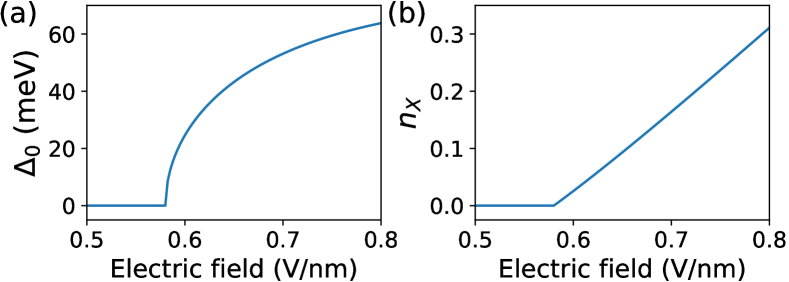
Figure 6: Gap-equation calculation. (a) Exciton order parameter $\Delta_{0}=\Delta_{\tau,\mathbf{k}=\mathbf{0}}$ and (b) exciton density $n_{\text{X}}$ v.s. electric-field strength $\mathcal{F}_{z}$.

The equilibrium exciton condensate can be described by the Bardeen-Cooper-Schrieffer (BCS)-like wavefunction

$$|{\Phi_{\text{BCS}}}\rangle=\prod_{\tau,\mathbf{k}}\big{(}u_{\tau,\mathbf{k}}+v_{\tau,\mathbf{k}}\hat{d}^{\dagger}_{\tau,\mathbf{k}}\hat{c}^{\dagger}_{-\mathbf{k}}\big{)}|{\Phi_{\text{HF}}}\rangle,$$ (36)

where $u_{\tau,\mathbf{k}}$ and $v_{\tau,\mathbf{k}}$ are variational coefficients subject to the normalization condition $u_{\tau,\mathbf{k}}^{2}+v_{\tau,\mathbf{k}}^{2}=1$jerome1967excitonic ; comte1982exciton . The variational coefficients can be solved as $u^{2}_{\tau,\mathbf{k}}=\left(1+{{\Xi}_{\tau,\mathbf{k}}}/{\mathcal{E}_{\tau,\mathbf{k}}}\right)/2$, $v^{2}_{\tau,\mathbf{k}}=\left(1-{{\Xi}_{\tau,\mathbf{k}}}/{\mathcal{E}_{\tau,\mathbf{k}}}\right)/2$, where $\mathcal{E}_{\tau,\mathbf{k}}=\sqrt{|{\Xi}_{\tau,\mathbf{k}}|^{2}+|\Delta_{\tau,\mathbf{k}}|^{2}}$ and ${\Xi}_{\tau,\mathbf{k}}=\big{(}\varepsilon^{\text{e}}_{-\mathbf{k}}+\varepsilon^{\text{h}}_{\tau,\mathbf{k}}\big{)}/2$. The exciton density is given by $n_{\text{X}}=\sum_{\tau,\mathbf{k}}v^{2}_{{\tau},\mathbf{k}}/N$, and the exciton order parameter $\Delta_{\tau,\mathbf{k}}$ can be solved from the gap equation (also see Appendix B.1)

$$\Delta_{\tau,\mathbf{k}}=\frac{1}{2S}\sum_{\mathbf{k}^{\prime}}\frac{W^{\text{eh}}_{\mathbf{k}-\mathbf{k}^{\prime}}\Delta_{\tau,\mathbf{k}^{\prime}}}{\mathcal{E}_{\tau,\mathbf{k}^{\prime}}}.$$ (37)

The results of the gap-equation calculation are shown in Fig. 6. The exciton condensate is formed at the electric-field strength of about $0.58$ V/nm, which is lower than the observed value $0.66$ V/nm at the topological phase transitionexp0 . The additional electric-field strength is required for the equilibrium exciton condensate to become a new stable state by replacing the Mott-insulator state.

IV.2 Survival of the Chern band

Since the hole-occupied moiré band is the Chern band in the $\text{MoTe}_{2}$ layer, it is essential to be aware of the possibility that the topology of the hole-occupied moiré band could be altered in the presence of the exciton condensate. To clarify that, we consider the quasiparticle Green’s function for the exciton condensatejerome1967excitonic ; zittartz1967theory ; chu1996theory

$${\mathcal{G}}_{\tau,\mathbf{k}}(\bar{t}) \equiv -\begin{pmatrix}\langle{\hat{\mathcal{T}}\hat{c}_{-\mathbf{k}}(0)\hat{c}^{\dagger}_{-\mathbf{k}}(\bar{t})}\rangle&\langle{\hat{\mathcal{T}}\hat{c}^{\dagger}_{-\mathbf{k}}(\bar{t})\hat{d}^{\dagger}_{\tau,\mathbf{k}}(0)}\rangle\\ \langle{\hat{\mathcal{T}}\hat{d}_{\tau,\mathbf{k}}(\bar{t})\hat{c}_{-\mathbf{k}}(0)}\rangle&\langle{\hat{\mathcal{T}}\hat{d}_{\tau,\mathbf{k}}(\bar{t})\hat{d}^{\dagger}_{\tau,\mathbf{k}}(0)}\rangle\end{pmatrix}.$$

By a Fourier transform $\mathcal{G}_{\tau,\mathbf{k}}(\mathtt{i}\omega_{\nu})=\frac{1}{\beta}\int^{\beta}_{0}e^{\mathtt{i}\omega_{\nu}\bar{t}}{\mathcal{G}}_{\tau,\mathbf{k}}(\bar{t})\text{d}\bar{t}$, with $\beta$ the inverse temperature and $\omega_{\nu}=(2\nu+1)\pi/\beta$, the quasiparticle Green’s function can be solved as

$$\tilde{\mathcal{G}}^{-1}_{\tau,\mathbf{k}}(\mathtt{i}\omega) = \begin{pmatrix}\mathtt{i}\omega+\varepsilon^{\text{e}}_{-\mathbf{k}}&-\Delta_{\tau,\mathbf{k}}\\ -\Delta_{\tau,\mathbf{k}}&\mathtt{i}\omega-\varepsilon^{\text{h}}_{\tau,\mathbf{k}}\end{pmatrix}.$$ (39)

The electron creation and annihilation operators can be replaced by the hole creation and annihilation operators by $\hat{c}^{\dagger}_{-\mathbf{k}}=\hat{d}_{\mathbf{k}}$, $\hat{c}_{-\mathbf{k}}=\hat{d}^{\dagger}_{\mathbf{k}}$. With including the valence bands in the $\text{MoTe}_{2}$ layer, the quasiparticle Green’s function can be generalized by the formulation ${\mathcal{G}}_{nm,\mathbf{k}}(\bar{t})\equiv-\langle{\hat{\mathcal{T}}\hat{d}_{n\mathbf{k}}(\bar{t})\hat{d}^{\dagger}_{m\mathbf{k}}(0)}\rangle$, with $n$, $m$ indexing different valence bands. This hole Green’s function satisfies a Ward-Takahashi identitychu1996theory , and thus the Chern number of the hole bands can also be calculated by Eq. (23). Therefore, based on the Green’s function given in Eq. (39), the effect of forming an exciton condensate on the band structure can be realized as the hybridization between the unfilled valence band (hole-occupied band) in the $\text{MoTe}_{2}$ layer and the valence bands in the $\text{WSe}_{2}$ layer. The topology of the Chern band will be altered only if $2{\Xi}_{\tau,\mathbf{k}}\leq\Delta_{\tau,\mathbf{k}}$, in which a band inversion could occur. Since $2{\Xi}_{\tau,\mathbf{k}}>\Delta_{\tau,\mathbf{k}}$ can be ensured by $\tilde{D}>\Delta_{0}$ as shown in Fig. 6 (a), the survival of the Chern band with the exciton condensate is ensured.

IV.3 Exciton ferromagnetism

In this section, we argue that an in-plane ferromagnetic order can be induced by exciton condensation and exciton-exciton interaction, and the in-plane ferromagnetic exchange field in the continuum model is contributed from the ferromagnetic order. Note that the moiré periodicity and the intralayer Coulomb repulsion have not been considered in the EHS Hamiltonian in Eq. (32). The moiré periodicity and the Coulomb repulsion can lead to the localization of an exciton in each moiré unit cell. Such an effect on the exciton condensate can be described by the excitonic Bose-Hubbard (EBH) Hamiltonianlagoin2021key ; remez2021dark ; gotting2022moir ,

$$\hat{\mathcal{H}}_{\text{EBH}} = -t\sum_{\tau,\langle{\mathbf{R},\mathbf{R}^{\prime}}\rangle}\hat{x}^{\dagger}_{\tau,\mathbf{R}}\hat{x}_{\tau,\mathbf{R}^{\prime}}+U\sum_{\mathbf{R}}\hat{x}^{\dagger}_{+,\mathbf{R}}\hat{x}^{\dagger}_{-,\mathbf{R}}\hat{x}_{-,\mathbf{R}}\hat{x}_{+,\mathbf{R}}$$ (40)

$$+U^{\prime}\sum_{\tau,\mathbf{R}}\hat{x}^{\dagger}_{\tau,\mathbf{R}}\hat{x}_{\tau,\mathbf{R}}(\hat{x}^{\dagger}_{\tau,\mathbf{R}}\hat{x}_{\tau,\mathbf{R}}-1),$$

where $\hat{x}^{\dagger}_{\tau,\mathbf{R}}=\frac{1}{\sqrt{N}}\sum_{\mathbf{K}}{e^{-\mathtt{i}\mathbf{K}\cdot\mathbf{R}}}\hat{X}^{\dagger}_{\tau,\mathbf{K}}$ is the exciton creation operator on the moiré unit cell at $\mathbf{R}$ site, with $\hat{X}^{\dagger}_{\tau,\mathbf{K}}=\sum_{\mathbf{k}}{\Psi}_{\tau,\mathbf{k},\mathbf{K}}\hat{d}^{\dagger}_{\tau,\mathbf{k}+\mathbf{K}}\hat{c}^{\dagger}_{-\mathbf{k}}$ and ${\Psi}_{\tau,\mathbf{k},\mathbf{K}}$ the wavefunction for the interlayer exciton in the moiré potential, $t$ is the nearest-neighbor hopping coupling, $U$ is the intervalley on-site repulsion, and $U^{\prime}$ is the intravalley on-site repulsion. The filling number of each moiré unit cell is given by the exciton density $n_{\text{X}}$. Since the exciton condensate is a BEC, the condensate can be assumed to be fragmented and distributed equally throughout the moiré superlatticemueller2006fragmentation ; ueda2010fundamentals . The exciton condensate can then be described by a rescaled EBH Hamiltonian with $\hat{x}_{\tau,\mathbf{R}}\rightarrow\sqrt{n_{\text{X}}}\hat{\tilde{x}}_{\tau,\mathbf{R}}$, $t\rightarrow\tilde{t}$, $U\rightarrow\tilde{U}/n_{\text{X}}$, $U^{\prime}\rightarrow\tilde{U}^{\prime}/{n}_{\text{X}}$, $\hat{\mathcal{H}}_{\text{EBH}}\rightarrow{n}_{\text{X}}\hat{\tilde{\mathcal{H}}}_{\text{EBH}}$ and the filling of the moiré superlattice becomes one exciton per unit cell. If $|\tilde{t}|\ll\tilde{U},\tilde{U}^{\prime}$, the EBH Hamiltonian with the filling number being one can be approximated by the anisotropic Heisenberg (XXZ) Hamiltoniankuklov2003counterflow ; altman2003phase ; duan2003controlling ; he2012quantum

$$\hat{\mathcal{H}}_{\text{XXZ}}=\sum_{\langle{\mathbf{R},\mathbf{R}^{\prime}}\rangle}\left[J_{z}\hat{\mathcal{S}}^{z}_{\mathbf{R}}\hat{\mathcal{S}}^{z}_{\mathbf{R}^{\prime}}-J_{\perp}\left(\hat{\mathcal{S}}^{x}_{\mathbf{R}}\hat{\mathcal{S}}^{x}_{\mathbf{R}^{\prime}}+\hat{\mathcal{S}}^{y}_{\mathbf{R}}\hat{\mathcal{S}}^{y}_{\mathbf{R}^{\prime}}\right)\right],$$

with $J_{z}=4\tilde{t}^{2}/\tilde{U}-4\tilde{t}^{2}/\tilde{U}^{\prime}$, $J_{\perp}=4\tilde{t}^{2}/\tilde{U}$ and $\hat{\mathcal{S}}^{x,y,z}_{\mathbf{R}}$ being pseudospin operators spanned by the basis $|{\tau}=\pm\rangle$. The model exhibits a transverse ferromagnetic order if $J_{\perp}>J_{z}$he2012quantum ; kosterlitz1973ordering . The ferromagnetic order induces TRS breaking and the in-plane ferromagnetic exchange field in the continuum model. It is estimated that $U\simeq U^{\prime}\simeq e^{2}/(\epsilon_{\text{r}}a_{\text{M}})\simeq 70$ meV, $t\simeq 0.015U\simeq 1$ meVgotting2022moir , and $n_{\text{X}}\simeq 0.10$ at the QAH state. We get $\tilde{U}=Un_{\text{X}}\simeq 7.0$ meV, $J_{\perp}\simeq 0.63$ meV, and $J_{z}\simeq{0}$ meV. The Berezinskii-Kosterlitz-Thouless (BKT) temperaturekosterlitz1973ordering in a triangular lattice is estimated to be about $T_{\text{BKT}}\simeq(1/0.69)J_{\perp}/(2k_{\text{B}})$butera1994high , which gives $T_{\text{BKT}}\simeq 5$ K. This scale is consistent with the observed Curie temperature for the ferromagnetic transitionexp0 . The ferromagnetic exchange field can be obtained from the mean-field approximation of the XXZ model

$$\hat{\mathcal{H}}_{\text{XXZ}} \simeq (J_{\perp}/2)\sum_{\langle{\mathbf{R},\mathbf{R}^{\prime}}\rangle}\left(\langle\hat{\mathcal{S}}^{+}_{\mathbf{R}}\rangle\langle\hat{\mathcal{S}}^{-}_{\mathbf{R}^{\prime}}\rangle+\langle\hat{\mathcal{S}}^{-}_{\mathbf{R}}\rangle\langle\hat{\mathcal{S}}^{+}_{\mathbf{R}^{\prime}}\rangle\right)$$ (42)

$$-J_{\perp}\sum_{\langle{\mathbf{R},\mathbf{R}^{\prime}}\rangle}\left(\hat{\mathcal{S}}^{+}_{\mathbf{R}}\langle\hat{\mathcal{S}}^{-}_{\mathbf{R}^{\prime}}\rangle+\hat{\mathcal{S}}^{-}_{\mathbf{R}}\langle\hat{\mathcal{S}}^{+}_{\mathbf{R}^{\prime}}\rangle\right),$$

with $\hat{\mathcal{S}}^{\pm}_{\mathbf{R}}=\hat{\mathcal{S}}^{x}_{\mathbf{R}}\pm\mathtt{i}\hat{\mathcal{S}}^{y}_{\mathbf{R}}=\hat{x}^{\dagger}_{\pm,\mathbf{R}}\hat{x}_{\mp,\mathbf{R}}$. The in-plane ferromagnetic magnetization can be estimated by $M_{\perp}\simeq zJ_{\perp}$ with $z$ the coordination number and $z=6$ for triangular lattices. The value is estimated to be $M_{\perp}\simeq 3.8$ meV. This value of the ferromagnetic magnetization is at the same scale as our assumed values in the calculations in Sec. III.3, but it is smaller than the value required for the topological nontrivial texture in Fig. 5 (e) to show up without a valley polarization of holes. The discrepancy might be caused by the roughness of the present estimation or the lack of considering long-range interaction for both the Hartree-Fock calculation and exciton ferromagnetism. We will return to the topic in future studies to improve the estimation.

IV.4 Exciton Mott transition

With a denser population of excitons under a higher electric field, the correlation-induced screening effect and Pauli-blocking effect may cause the dissociation of excitons and the formation of electron-hole plasma. The mechanism is known as exciton Mott transitionhanamura1977condensation ; keldysh1986electron ; zimmermann1988nonlinear ; asano2014exciton ; fogler2014high ; rustagi2018theoretical . A Mott density $\rho_{\text{Mott}}$ is defined as the critical exciton density in which the dissociation of excitons occurs. Two different theoretical schemes have been proposed to estimate the Mott density. One theoretical scheme suggests that the Mott density is the exciton density in which exciton wavefunctions begin to overlap mutually. For two-dimensional systems, the Mott density is estimated to be $\rho_{\text{Mott}}a^{2}_{\text{X}}\simeq 0.3\sim 0.7$. This scheme has been supported by using quantum Monte-Carlo calculationsde2002excitonic ; rios2018evidence . The other theoretical scheme assumes that the Mott density is reached as the electron-hole-excitation-induced band-gap renormalization energy is larger than the exciton binding energy. The Mott density estimated by this schemehanamura1977condensation ; zimmermann1988nonlinear ; asano2014exciton ; rustagi2018theoretical is about $\rho_{\text{Mott}}a^{2}_{\text{X}}\simeq 0.02\sim 0.08$. While both theoretical schemes have gathered supporters, recent experiments on exciton Mott transition in the moiré-bilayer system suggest $\rho_{\text{Mott}}a^{2}_{\text{X}}\simeq 0.01\sim 0.07$wang2021diffusivity ; siday2022ultrafast , which strongly supports the second scheme.

For MoTe₂/WSe₂ moiré heterobilayers, if $\rho_{\text{Mott}}a^{2}_{\text{X}}\simeq 0.02$ is assumed, the exciton density per moiré unit cell at the exciton Mott transition is estimated to be $n_{\text{X}}=\rho_{\text{Mott}}\bar{S}\simeq 0.02\times(\sqrt{3}/2)\times a^{2}_{\text{M}}/a^{2}_{\text{X}}\simeq 0.17$, which can be reached by the imposed electric-field strength $0.70$ V/nm according to Fig. 6. (b). This estimation is consistent with the observed electric field in which the metallic phases show up in both AA-stacked and AB-stacked MoTe₂/WSe₂ heterobilayersexp0 ; li2021continuous . At low temperatures, the exciton Mott transition is a quantum phase transition between BEC-like exciton-gas condensation and BCS-like electron-hole-liquid condensationbronold2006possibility ; kremp2008quantum . Since the BEC-to-BCS transition is known as a continuous crossoverbronold2006possibility ; kremp2008quantum and the electron-hole-liquid condensate can also be seen as a two-component Fermi liquidhanamura1977condensation , the observed continuous insulator-to-metal transition in MoTe₂/WSe₂ heterobilayers at low temperaturesexp0 ; li2021continuous could be explained by the exciton Mott transition.

V Discussions and Conclusion

The consistency between the present theory and experimental observations is discussed sequentially regarding the enumerated list in the introduction:

1. The continuum model gives the bandwidth $E_{W}=43$ meV for the highest moiré band in the MoTe₂ layer and the contact-interaction energy $U=70$ meV for the on-site Coulomb repulsion. Since $U>E_{W}$, the equilibrium state is a Mott-insulator state in low electric fields. An interlayer-exciton condensate is formed at $\nu=1$ hole filling and a certain electric field. A correlated insulating state composed of the hole-occupied band and the exciton condensate becomes a new stable phase while competing with the Mott-insulator state, such that the band-structure picture can still be available beyond the electric-field strength.

2. The valence-band energy offset is assumed to be $D=280$ meV, which is not far from the observed value of $300$ meV. At the topological phase transition, the valence-band energy offset is reduced to $\tilde{D}=108$ meV, which is still much larger than the bandwidth $E_{W}=43$ meV for the highest moiré band in the MoTe₂ layer. Therefore, the band inversion between the highest moiré band in the MoTe₂ layer and the highest moiré band in the WSe₂ layer can not be achieved with the out-of-plane electric fields imposed in the experiment. In our theory, the band inversion is intrinsic. The highest two moiré hole bands with opposite valley numbers in the MoTe₂ layer cross with each other, and the gap opening is attributed to the formation of an in-plane $120^{\circ}$-Néel order and an in-plane ferromagnetic order. The Néel order ensures the insulating gap. The Chern band emerges along with the formation of the ferromagnetic order. Since the gap is opened before and after the topological phase transition, there is no charge gap closure.

3. An in-plane ferromagnetic order emerges in the moiré superlattice under sufficient out-of-plane electric fields due to exciton condensation. The exciton ferromagnetism can be demonstrated by an EBH model and BKT transition. The ferromagnetic transition temperature is estimated to be $5$ K, which is coincident with the observation.

4. The exciton Mott transition, a phase transition from exciton liquid to electron-hole plasma, could occur as the electric-field strength reaches about $0.70$ V/nm. At low temperatures, the exciton liquid becomes a BEC and the electron-hole plasma becomes a BCS-like state known as an electron-hole condensate, which can be seen as a two-component Fermi liquid. The continuous insulator-to-metal transition and the Fermi liquid behavior at low temperatures could be explained by the excitonic BCS-BEC crossover.

5. The spin-polarized or valley-coherent QAH ground state across two layers can be interpreted by interlayer-exciton condensation. Based on band-edge energies in Eq. (8) and Fig. 4 (f), it is found that the hole-occupied Chern band in the MoTe₂ layer is mainly composed of the valley-polarized hole band with $\tau=+$ as $M_{z}>0$ or mainly composed of the valley-polarized hole band with $\tau=-$ as $M_{z}<0$. The exciton is formed by the vertical hole transition from the MoTe₂ layer to the WSe₂ layer. By examining the band structures of the moiré heterobilayers in Fig. 2, the vertical transition from the valley-polarized hole band generates a valley-coherent exciton, where the electron and the hole reside in different valleys. Based on the spin-valley coupling shown in Fig. 1 (c), the valley-coherent exciton is spin polarized. Additionally, by the layer-selected Zeeman shifts shown in Eq. (7) and Eq. (8), the spin-aligned MCD signal for exciton polarons in two layers can be interpreted.

6. Full spin-valley polarization is not required for quantized Hall transport since the QAH state is generated by the in-plane ferromagnetic order, not field-induced valley polarization of holes. The observed canted spin texture can be explained by the coexistence of the in-plane $120^{\circ}$-Néel order and the field-induced valley polarization in the MoTe₂ layer as the discussion in Sec. III.2.

7. The QSH effect at $\nu=2$ hole filling and the band-to-QSH transition are not studied in this work. This effect and this transition have been interpreted by Kane-Mele physicsexp2 . Our theory does not exclude the interpretation. It is worth noting that the valence-band energy offset ($280$ meV) could be compensated by Coulomb-interaction-driven band-energy renormalization, which contributes about $-110$ meV energy shift. Since the bandwidth of the hole band in the MoTe₂ layer has contributed about $-40$ meV energy shift, the topological phase transition could occur at $-130$ meV electric-field-induced energy shift ($0.50$ V/nm electric-field strength).

Through these discussions, the consistency between the present theory and the experimental observations is argued. Discussions about the Mott insulating state and exciton Mott transition could also contribute to the study of the continuum phase transition found in AA-stacked MoTe₂/WSe₂ heterobilayers.

An additional argument to support the present theory is the sparseness of QAH states being found in transition metal dichalcogenide (TMDC) moiré heterobilayers. In fact, to the best of the authors’ knowledge, except AB-stacked MoTe₂/WSe₂ heterobilayers, no QAH state has been found in other TMDC moiré heterobilayers. Several theories that explain the QAH effect in AB-stacked MoTe₂/WSe₂ heterobilayers could predict a wide distribution of QAH states in TMDC moiré heterobilayers. Nevertheless, it seems to be not the case. In our theory, the sparseness can be attributed to the restricted parametrization for the present model to meet the conditions that exciton ferromagnetism occurs and the ferromagnetic phase transition precedes the exciton Mott transition.

In conclusion, a theory to explain the QAH effect and the topological phase transition in AB-stacked MoTe₂/WSe₂ heterobilayers is provided. The consistency between the theory and experimental observations is argued. This work may contribute a new viewpoint to search QAH insulators among correlated materials and a new route to study topological orders in moiré materials.

Appendix A Moiré band-structure calculation

The method to calculate moiré band structures for the continuum model of AB-stacked $\text{MoTe}_{2}$/$\text{WSe}_{2}$ heterobilayers is given in this section. In Sec. A.1, the plane-wave method to solve moiré band structures is introduced. In Sec. A.2, the Hartree-Fock approximation for band structure calculation is reviewed.

A.1 Plane-wave method

The single-particle wavefunction of a carrier in the moiré superlattice can be expanded in terms of plane-wave basis functions as

$$\psi_{n\mathbf{k}}(\mathbf{r})=\sum_{{\alpha}}u_{n\mathbf{k}}\phi_{\mathbf{G}_{\alpha},\mathbf{k}}(\mathbf{r}),$$ (43)

where $\phi_{\mathbf{G}_{\alpha},\mathbf{k}}(\mathbf{r})$ denotes a plane-wave basis function and $u_{{\alpha},n\mathbf{k}}$ is the the expansion coefficient. The plane-wave basis function is written as

$$\phi_{\mathbf{G},\mathbf{k}}(\mathbf{r})=e^{\mathtt{i}\left(\mathbf{k}-\mathbf{G}\right)\cdot\mathbf{r}}/\sqrt{S},$$ (44)

with $S=N(\sqrt{3}/2)a^{2}_{\text{M}}$ the area of the moiré lattice. By using the plane-wave expansion, the Hamiltonian matrix is given by $\langle a,\mathbf{G}_{1}|\tilde{H}_{\mathbf{k}}|b,\mathbf{G}_{2}\rangle=\int\phi^{*}_{\mathbf{G}_{1},\mathbf{k}}(\mathbf{r})H_{ab}(\mathbf{r})\phi_{\mathbf{G}_{2},\mathbf{k}}(\mathbf{r})\text{d}^{2}r$ and the diagonal part is given by

$$\langle a,\mathbf{G}_{\alpha}|\tilde{H}_{\mathbf{k}}|a,\mathbf{G}_{\beta}\rangle = \delta_{\alpha\beta}\frac{|\mathbf{k}-\mathbf{G}_{\alpha}-\tau_{a}\boldsymbol{\kappa}_{l_{a}}|^{2}}{2m_{l_{a}}}$$ (45)

$$-\langle a,\mathbf{G}_{\alpha}|\tilde{V}_{l_{a},\mathbf{k}}|a,\mathbf{G}_{\beta}\rangle,$$

with $\langle a,\mathbf{G}_{\alpha}|\tilde{V}_{l_{a},\mathbf{k}}|a,\mathbf{G}_{\beta}\rangle=-\mathtt{i}V\sum_{j}(-1)^{l_{a}+j}\delta(\mathbf{G}_{\alpha}-\mathbf{G}_{\beta}-\boldsymbol{g}_{j})$. The off-diagonal Hamiltonian matrix element is given by

$$\langle a,\mathbf{G}_{\alpha}|\tilde{H}_{\mathbf{k}}|b,\mathbf{G}_{\beta}\rangle = w\delta_{\tau_{a},\tau_{b}}\delta_{l_{a},l_{b}+1}\Big{[}\delta(\mathbf{G}_{\alpha}-\mathbf{G}_{\beta})$$ (46)

$$+\sum_{j=1,2}\delta(\mathbf{G}_{\alpha}-\mathbf{G}_{\beta}-\tau_{a}\boldsymbol{g}_{j})\Big{]}$$

$$+w\delta_{\tau_{a},\tau_{b}}\delta_{l_{a}+1,l_{b}}\Big{[}\delta(\mathbf{G}_{\alpha}-\mathbf{G}_{\beta})$$

$$+\sum_{j=1,2}\delta(\mathbf{G}_{\alpha}-\mathbf{G}_{\beta}+\tau_{a}\boldsymbol{g}_{j})\Big{]}.\hskip 17.22217pt$$

A.2 Hartree-Fock approximation

Given the many-particle Hamiltonian for multi-component particle fields in Eq. (22), the quasiparticle creation and annihilation operators can be transformed as $\hat{\Psi}^{\dagger}_{a}(\mathbf{r})=\sum_{n\mathbf{k}}\psi^{*}_{a,n\mathbf{k}}(\mathbf{r})\hat{d}^{\dagger}_{n\mathbf{k}}$, $\hat{\Psi}_{a}(\mathbf{r})=\sum_{n\mathbf{k}}\psi_{a,n\mathbf{k}}(\mathbf{r})\hat{d}_{n\mathbf{k}}$, with $\psi_{a,n\mathbf{k}}(\mathbf{r})$ the quasiparticle wavefunction. By using the variational method, it is found that the quasiparticle wavefunction can be solved by the Hartree-Fock equation

$$\sum_{b}\int F_{ab}(\mathbf{r}_{1},\mathbf{r}_{2})\psi_{b,n\mathbf{k}}(\mathbf{r}_{2})\text{d}^{2}r_{2}=\varepsilon_{n\mathbf{k}}\psi_{a,n\mathbf{k}}(\mathbf{r}_{1}),\hskip 8.61108pt$$ (47)

where $n$ is the band index, $\varepsilon_{n\mathbf{k}}$ is the quasiparticle energy. The Fock operator is defined by

$$F_{ab}(\mathbf{r}_{1},\mathbf{r}_{2}) = \delta(\mathbf{r}_{1}-\mathbf{r}_{2})\left[H_{ab}(\mathbf{r}_{1})+\delta_{ab}K_{aa}(\mathbf{r}_{1})\right]$$ (48)

$$-J_{ab}(\mathbf{r}_{1},\mathbf{r}_{2}),$$

where $K_{aa}(\mathbf{r}_{1})\equiv\sum_{c}\int{W}_{ac}(\mathbf{r}_{13})\rho_{cc}(\mathbf{r}_{3},\mathbf{r}_{3})\text{d}^{2}r_{3}$ is the Coulomb operator, $J_{ab}(\mathbf{r}_{1},\mathbf{r}_{2})\equiv W_{ab}(\mathbf{r}_{12})\rho_{ba}(\mathbf{r}_{2},\mathbf{r}_{1})$ is the exchange operator, and

$$\rho_{ab}(\mathbf{r}_{1},\mathbf{r}_{2}) = \sum_{n\mathbf{k}}n_{n\mathbf{k}}\psi_{a,n\mathbf{k}}(\mathbf{r}_{1})\psi^{*}_{b,n\mathbf{k}}(\mathbf{r}_{2})$$ (49)

is the density-matrix operator, where $n_{n\mathbf{k}}=\langle{\hat{d}^{\dagger}_{n\mathbf{k}}\hat{d}_{n\mathbf{k}}}\rangle$ is the occupation number of charges in the band $n$ with the momentum $\mathbf{k}$.

By using the plane-wave method, the wavefunction coefficient can be obtained by solving the Hartree-Fock equation $\tilde{F}_{\mathbf{k}}u_{n\mathbf{k}}=\varepsilon_{n\mathbf{k}}u_{n\mathbf{k}}$. The Fock matrix is given by

$$\langle a,\mathbf{G}_{\alpha}|\tilde{F}_{\mathbf{k}}|b,\mathbf{G}_{\beta}\rangle = \langle a,\mathbf{G}_{\alpha}|\tilde{H}_{\mathbf{k}}|b,\mathbf{G}_{\beta}\rangle-\langle a,\mathbf{G}_{\alpha}|\tilde{J}_{\mathbf{k}}|b,\mathbf{G}_{\beta}\rangle$$ (50)

$$+\delta_{ab}\langle a,\mathbf{G}_{\alpha}|\tilde{K}_{\mathbf{k}}|a,\mathbf{G}_{\beta}\rangle.$$

The Coulomb integral is given by

$$\langle a,\mathbf{G}_{\alpha}|\tilde{K}_{\mathbf{k}}|a,\mathbf{G}_{\beta}\rangle = \sum_{\mathbf{q},\mathbf{G},c}\langle c,\mathbf{G}+\mathbf{G}_{\alpha}|\tilde{P}_{\mathbf{q}}|c,\mathbf{G}+\mathbf{G}_{\beta}\rangle$$ (51)

$$\times{\tilde{W}_{ac}(\mathbf{G}_{\alpha}-\mathbf{G}_{\beta})}/S,$$

and the exchange integral is given by

$$\langle a,\mathbf{G}_{\alpha}|\tilde{J}_{\mathbf{k}}|b,\mathbf{G}_{\beta}\rangle = \sum_{\mathbf{q},\mathbf{G}}\langle a,\mathbf{G}+\mathbf{G}_{\alpha}|\tilde{P}_{\mathbf{q}}|b,\mathbf{G}+\mathbf{G}_{\beta}\rangle$$ (52)

$$\times\tilde{W}_{ab}(\mathbf{G}+\mathbf{k}-\mathbf{q})/S,$$

where

$$\langle a,\mathbf{G}_{\alpha}|\tilde{P}_{\mathbf{k}}|b,\mathbf{G}_{\beta}\rangle=\sum_{n}n_{n\mathbf{k}}u_{(a,\mathbf{G}_{\alpha}),n\mathbf{k}}u^{*}_{(b,\mathbf{G}_{\beta}),n\mathbf{k}}\hskip 17.22217pt$$ (53)

is the single-particle projection matrix and $\tilde{W}_{ab}(\mathbf{k})=\int\exp\left({-\mathtt{i}\mathbf{k}\cdot\mathbf{r}}\right)W_{ab}(\mathbf{r})\text{d}^{2}r$ is the screened Coulomb potential.

Appendix B Formulations for exciton condensation

In this section, theory of exciton condensation is revisited based on referencesjerome1967excitonic ; zittartz1967theory ; halperin1968excitonic ; keldysh1968collective ; comte1982exciton ; nozieres1982exciton ; fernandez1997spin ; chu1996theory ; wu2015theory . In Sec. B.1, the gap equation for exciton condensates is derived. In Sec. B.2, the variational method to solve the exciton binding energy is introduced. In Sec. B.3, the conditions of excitonic instability are discussed.

B.1 Gap equation

Exciton condensation can be described by the EHS Hamiltonian in Eq. (32) with a more general form of the combination of electron-band and hole-band dispersion

$$\varepsilon^{\text{e}}_{-\mathbf{k}}+\varepsilon^{\text{h}}_{\tau,\mathbf{k}}=\tilde{D}+\frac{k^{2}}{2\mu_{\text{X}}},$$ (54)

where $\mu_{\text{X}}=m_{\text{e}}m_{\text{h}}/(m_{\text{e}}+m_{\text{h}})$ is the reduced mass. The variational state for a exciton condensate is assumed to be the following BCS state $|{\Phi_{\text{BCS}}}\rangle=\prod_{\tau,\mathbf{k}}\left(u_{\tau,\mathbf{k}}+v_{\tau,\mathbf{k}}\hat{d}^{\dagger}_{\tau,\mathbf{k}}\hat{c}^{\dagger}_{-\mathbf{k}}\right)|{\Phi_{\text{HF}}}\rangle$, where $u_{\tau,\mathbf{k}}$ and $v_{\tau,\mathbf{k}}$ are variational coefficients subject to the normalization condition $u_{\tau,\mathbf{k}}^{2}+v_{\tau,\mathbf{k}}^{2}=1$. Note that

$$\frac{\delta u_{\tau,\mathbf{k}}}{\delta v_{\tau^{\prime},\mathbf{k}^{\prime}}}=-\delta_{\tau,\tau^{\prime}}\delta_{\mathbf{k},\mathbf{k}^{\prime}}\frac{v_{\tau,\mathbf{k}}}{u_{\tau,\mathbf{k}}}.$$ (55)

The expectation of the Hamiltonian is given by

$$\langle{\hat{\mathcal{H}}_{\text{EHS}}}\rangle = \sum_{\tau,\mathbf{k}}\left(\varepsilon^{\text{e}}_{-\mathbf{k}}+\varepsilon^{\text{h}}_{\tau,\mathbf{k}}\right)v_{\tau,\mathbf{k}}^{2}$$ (56)

$$-\sum_{\tau,\mathbf{k}\neq\mathbf{k}^{\prime}}\frac{W^{\text{eh}}_{\mathbf{k}^{\prime}-\mathbf{k}}}{S}v_{\tau,\mathbf{k}^{\prime}}v_{\tau,\mathbf{k}}u_{\tau,\mathbf{k}}u_{\tau,\mathbf{k}^{\prime}}.$$

The variation of the energy expectation value is given by

$$\frac{\delta\langle{\hat{\mathcal{H}}_{\text{EHS}}}\rangle}{\delta v_{\tau,\mathbf{k}}} = 2\left(\varepsilon^{\text{e}}_{-\mathbf{k}}+\varepsilon^{\text{h}}_{\tau,\mathbf{k}}\right)v_{\tau,\mathbf{k}}$$

$$-2\sum_{\mathbf{k}^{\prime}}\frac{W^{\text{eh}}_{\mathbf{k}-\mathbf{k}^{\prime}}}{S}v_{\tau,\mathbf{k}^{\prime}}u_{\tau,\mathbf{k}^{\prime}}\left(u_{\tau,\mathbf{k}}-\frac{v^{2}_{\tau,\mathbf{k}}}{u_{\tau,\mathbf{k}}}\right).$$

By variation ${\delta\langle{\hat{\mathcal{H}}_{\text{EHS}}}\rangle}/{\delta v_{\tau,\mathbf{k}}}=0$, and by assuming $\Delta_{\tau,\mathbf{k}}=(1/S)\sum_{\mathbf{k}^{\prime}}W^{\text{eh}}_{\mathbf{k}-\mathbf{k}^{\prime}}v_{\tau,\mathbf{k}^{\prime}}u_{\tau,\mathbf{k}^{\prime}}$, ${\Xi}_{\tau,\mathbf{k}}=\big{(}\varepsilon^{\text{e}}_{-\mathbf{k}}+\varepsilon^{\text{h}}_{\tau,\mathbf{k}}\big{)}/2$, we get $\big{(}2v_{\tau,\mathbf{k}}u_{\tau,\mathbf{k}}\big{)}{\Xi}_{\tau,\mathbf{k}}-\big{(}u^{2}_{\tau,\mathbf{k}}-v^{2}_{\tau,\mathbf{k}}\big{)}\Delta_{\tau,\mathbf{k}}=0$. By replacing $u_{\tau,\mathbf{k}}=\cos\theta_{\tau,\mathbf{k}}$ and $v_{\tau,\mathbf{k}}=\sin\theta_{\tau,\mathbf{k}}$, we find $\sin(2\theta_{\tau,\mathbf{k}}){\Xi}_{\tau,\mathbf{k}}=\cos(2\theta_{\tau,\mathbf{k}})\Delta_{\tau,\mathbf{k}}$ and $\cos(2\theta_{\tau,\mathbf{k}})={\Xi}_{\tau,\mathbf{k}}/\mathcal{E}_{\tau,\mathbf{k}}$, with $\mathcal{E}_{\tau,\mathbf{k}}=\sqrt{|{\Xi}_{\tau,\mathbf{k}}|^{2}+|\Delta_{\tau,\mathbf{k}}|^{2}}$. Therefore, we get

$$u^{2}_{\tau,\mathbf{k}}=\frac{1}{2}\left(1+\frac{{\Xi}_{\tau,\mathbf{k}}}{\mathcal{E}_{\tau,\mathbf{k}}}\right),\hskip 4.30554ptv^{2}_{\tau,\mathbf{k}}=\frac{1}{2}\left(1-\frac{{\Xi}_{\tau,\mathbf{k}}}{\mathcal{E}_{\tau,\mathbf{k}}}\right),$$ (58)

and $2v_{\tau,\mathbf{k}}u_{\tau,\mathbf{k}}=\sin(2\theta_{\tau,\mathbf{k}})=\Delta_{\tau,\mathbf{k}}/\mathcal{E}_{\tau,\mathbf{k}}$. The gap equation can be found as Eq. (37). By replacing the variational parameters, the exciton density is given by

$${n}_{\text{X}}=\frac{1}{N}\sum_{\tau,\mathbf{k}}v^{2}_{{\tau},\mathbf{k}}=\sum_{\tau,\mathbf{k}}\frac{1}{2N}\left(1-\frac{{\Xi}_{\tau,\mathbf{k}}}{\mathcal{E}_{\tau,\mathbf{k}}}\right).$$ (59)

B.2 Exciton binding energy

The variational method to solve the exciton banding energy is introduced in this section. Two-dimensional Slater-type orbitals (STOs) are used to expanded the variational exciton wavefunction. A more detailed discussion of this method can be found in Ref. mypaper0 . As the combination of electron and hole kinetic energies is assumed to be given by Eq. (54), the interlayer exciton wavefunction $\Psi_{I}(\mathbf{r})$ can be solved by the Schrödinger equation

$$\left[\tilde{D}-\frac{\nabla^{2}}{2\mu_{\text{X}}}-W(\mathbf{r})\right]\Psi_{I}(\mathbf{r})=E_{I}\Psi_{I}(\mathbf{r}).$$ (60)

The Fourier transform of the exciton wavefunction can be found by $\tilde{\Psi}_{I}({\mathbf{k}})=\int\;e^{-\mathtt{i}\mathbf{k}\cdot\mathbf{r}}\Psi_{I}(\mathbf{r})\text{d}^{2}r$. The exciton wavefunction can be expanded as

$$\tilde{\Psi}_{I}({\mathbf{k}})=\sum_{\alpha}\mathcal{U}_{\alpha,I}\tilde{\Phi}_{\alpha}(\mathbf{k}),$$ (61)

where $\mathcal{U}_{\alpha,I}$ is the wavefunction coefficient and $\tilde{\Phi}_{\alpha}(\mathbf{k})$ is the basis function. The exciton wavefunction coefficient can be solved by the eigenvalue equation

$$\sum_{\beta}\left(\mathcal{T}_{\alpha\beta}-\mathcal{W}_{\alpha\beta}\right)\mathcal{U}_{\beta,I}=E_{I}\sum_{\beta}\mathcal{O}_{\alpha\beta}\mathcal{U}_{\beta,I},$$ (62)

where $\mathcal{T}_{\alpha\beta}\equiv-[1/({2\mu_{\text{X}}})]\int\Phi^{*}_{\alpha}(\mathbf{r})\nabla^{2}\Phi_{\beta}(\mathbf{r})\text{d}^{2}{r}$, $\mathcal{W}_{\alpha\beta}\equiv\int{\Phi}^{*}_{\alpha}(\mathbf{r}){W}(\mathbf{r}){\Phi}_{\beta}(\mathbf{r})\text{d}^{2}r$, $\mathcal{O}_{\alpha\beta}\equiv\int\Phi^{*}_{\alpha}(\mathbf{r})\Phi_{\beta}(\mathbf{r})\text{d}^{2}{r}$ are the kinetic integral, the potential integral, and the overlap integral. By using an orthogonalization transformation $\bar{\mathcal{U}}_{\alpha,I}=\sum_{\beta}\mathcal{O}^{1/2}_{\alpha\beta}\mathcal{U}_{\beta,I}$, the eigenvalue equation becomes

$$\sum_{\beta}\Omega_{\alpha\beta}\bar{\mathcal{U}}_{\beta,I}=E_{I}\bar{\mathcal{U}}_{\beta,I},$$ (63)

with $\Omega_{\alpha\beta}=\sum_{\alpha^{\prime}\beta^{\prime}}\mathcal{O}^{-1/2}_{\alpha\alpha^{\prime}}\left(\mathcal{T}_{\alpha^{\prime}\beta^{\prime}}-\mathcal{W}_{\alpha^{\prime}\beta^{\prime}}\right)\mathcal{O}^{-1/2}_{\beta^{\prime}\beta}$.

To solve the exciton eigenvalue equation in Eq. (62), the basis function can be given by a two-dimensional STO, which is written as

$$\Phi_{\alpha}(\mathbf{r}) = \frac{e^{\mathtt{i}L_{\alpha}\varphi}}{\sqrt{2\pi}}r^{N_{\alpha}-1}e^{-\mathcal{Z}_{\alpha}r},$$ (64)

where $N_{\alpha}$, $L_{\alpha}$ are the principal quantum number and angular-momentum quantum number of the orbital $\Phi_{\alpha}$, $\mathcal{Z}_{\alpha}$ is the shielding constant, and $\varphi$ is the azimuth angle. Several different values of $\mathcal{Z}_{\alpha}$ can be used to find the optimum shape of the radial part of the wavefunction. The Fourier transform of the two-dimensional STO can be written as

$$\tilde{\Phi}_{\alpha}(\mathbf{k}) = \int\Phi_{\alpha}(\mathbf{r})e^{-\mathtt{i}\mathbf{k}\cdot\mathbf{r}}\text{d}^{2}r=\frac{e^{\mathtt{i}L_{\alpha}\varphi_{\mathbf{k}}}}{\sqrt{2\pi}}\tilde{\mathcal{R}}_{N_{\alpha},L_{\alpha}}(\mathcal{Z}_{\alpha},k),$$

where the radial function in momentum space can be obtained by the generating formula

$$\tilde{\mathcal{R}}_{N,L}(\mathcal{Z},k) = \frac{2\pi(-\mathtt{i})^{N}}{k^{N+1}}\frac{\text{d}^{N}}{\text{d}z^{N}}\frac{\left(z-\mathtt{i}\eta\sqrt{1-z^{2}}\right)^{|L|}}{\sqrt{1-z^{2}}}\Bigg{|}_{z=\mathtt{i}{\mathcal{Z}}/{k}},$$

with $\eta=L/|L|$. The kinetic integral is given by

$$\mathcal{T}_{\alpha\beta} = -\frac{\delta_{L_{\alpha},L_{\beta}}}{2\mu_{\text{X}}}\frac{(N_{\alpha}+N_{\beta}-1)!}{\left(\mathcal{Z}_{\alpha}+\mathcal{Z}_{\beta}\right)^{N_{\alpha}+N_{\beta}}}\Bigg{\{}(1-\delta_{N_{\beta},1})$$ (67)

$$\times\frac{\big{[}(N_{\beta}-1)^{2}-L_{\beta}^{2}\big{]}\left(\mathcal{Z}_{\alpha}+\mathcal{Z}_{\beta}\right)^{2}}{(N_{\alpha}+N_{\beta}-1)(N_{\alpha}+N_{\beta}-2)}$$

$$-\frac{\left[(2N_{\beta}-1)\mathcal{Z}_{\beta}\right]\left(\mathcal{Z}_{\alpha}+\mathcal{Z}_{\beta}\right)}{(N_{\alpha}+N_{\beta}-1)}+\mathcal{Z}^{2}_{\beta}\Bigg{\}}.$$

The overlap integral is given by

$$\mathcal{O}_{\alpha\beta} = \delta_{L_{\alpha},L_{\beta}}\frac{(N_{\alpha}+N_{\beta}-1)!}{(\mathcal{Z}_{\alpha}+\mathcal{Z}_{\beta})^{N_{\alpha}+N_{\beta}}}.$$ (68)

The potential integral is given by

$$\mathcal{W}_{\alpha\beta} = \frac{\delta_{L_{\alpha},L_{\beta}}}{(2\pi)^{2}}\int^{\infty}_{0}\tilde{\mathcal{R}}_{N_{\alpha}+N_{\beta}-1,0}(\mathcal{Z}_{\alpha}+\mathcal{Z}_{\beta},k)\tilde{W}(k)k\text{d}k.$$

The Coulomb potential can be given by $\tilde{W}(k)=W^{\text{eh}}_{\mathbf{k}}$. An exciton $I=(N,L)$ can be indicated by a principal quantum number $N$ and an angular momentum $L$, with $L$ being a constant for every orbital in the exciton wavefunction. In the present study, only $L=0$ is considered.

B.3 Conditions of excitonic instability

If the number of excitons is restricted to one, by a variation of the ground-state expectation value of the EHS Hamiltonian

$$\delta\left[\langle{\Phi|\hat{\mathcal{H}}_{\text{EHS}}|\Phi}\rangle-\lambda\left(N{n}_{\text{X}}-1\right)\right]/\delta{v}_{\tau,\mathbf{k}}=0,$$ (70)

with $\lambda$ the Lagrange multiplier, the BCS variational coefficient $v_{{\tau},\mathbf{k}}$ can be solved by

$$[k^{2}/(2\mu_{\text{X}})+E_{\text{X}}]v_{{\tau},\mathbf{k}}=\sum\nolimits_{\mathbf{k}^{\prime}}W^{\text{eh}}_{\mathbf{k}-\mathbf{k}^{\prime}}v_{{\tau},\mathbf{k}^{\prime}}/S,$$ (71)

where $E_{\text{X}}=\tilde{D}-\lambda$ is the exciton binding energy. By comparing Eq. 71 with the exciton equation in Eq. (60), the coefficient is equivalent to the ground-state exciton wavefunction ($v_{{\tau},\mathbf{k}}=\Psi_{I,\mathbf{k}}$ for $I=0$) under the condition. We define the excitonic instability to form condensation by the condition

$$\Delta_{\tau,\mathbf{k}}\neq{0}$$ (72)

for at least one $(\tau$, $\mathbf{k})$ state. In this section, we want to show that the necessary condition for the excitonic instability at zero temperature is $\tilde{D}\leq E_{\text{X}}$ and the sufficient condition is $\tilde{D}<E_{\text{X}}$, with $\tilde{D}$ being the effective band gap.

To prove the necessary condition, we can rewrite the gap equation by defining

$$\gamma_{\tau,\mathbf{k}}\equiv u_{\tau,\mathbf{k}}v_{\tau,\mathbf{k}}=\frac{\Delta_{\tau,\mathbf{k}}}{2\mathcal{E}_{\tau,\mathbf{k}}}.$$ (73)

The gap equation can be rewritten as $\gamma_{\tau,\mathbf{k}}=[{1}/({2\mathcal{E}_{\tau,\mathbf{k}}})]\sum_{\mathbf{k}^{\prime}}{W^{\text{eh}}_{\mathbf{k}-\mathbf{k}^{\prime}}}\gamma_{\tau,\mathbf{k}^{\prime}}/S$, and then it can become

$$2\mathcal{E}_{\tau,\mathbf{k}}\gamma_{\tau,\mathbf{k}}-\sum_{\mathbf{k}^{\prime}}\frac{W^{\text{eh}}_{\mathbf{k}-\mathbf{k}^{\prime}}}{S}\gamma_{\tau,\mathbf{k}^{\prime}}=0.$$ (74)

By using

$$\mathcal{E}_{\tau,\mathbf{k}} = \sqrt{|{\Xi}_{\tau,\mathbf{k}}|^{2}+|\Delta_{\tau,\mathbf{k}}|^{2}}=|{\Xi}_{\tau,\mathbf{k}}|\sqrt{1+|\Delta_{\tau,\mathbf{k}}|^{2}/|{\Xi}_{\tau,\mathbf{k}}|^{2}}$$ (75)

$$= |{\Xi}_{\tau,\mathbf{k}}|+g_{\tau,\mathbf{k}},$$

with $g_{\tau,\mathbf{k}}=|{\Xi}_{\tau,\mathbf{k}}|\big{(}\sqrt{1+{|\Delta_{\tau,\mathbf{k}}|^{2}}/{|{\Xi}_{\tau,\mathbf{k}}|^{2}}}-1\big{)}\geq{0}$, and assuming ${\Xi}_{\tau,\mathbf{k}}>0$, the gap equation becomes

$$2({\Xi}_{\tau,\mathbf{k}}+g_{\tau,\mathbf{k}})\gamma_{\tau,\mathbf{k}}-\sum_{\mathbf{k}^{\prime}}\frac{W^{\text{eh}}_{\mathbf{k}-\mathbf{k}^{\prime}}}{S}\gamma_{\tau,\mathbf{k}^{\prime}}=0.$$ (76)

By using Eq. (54), the gap equation can be rewritten as

$$\sum_{\mathbf{k}^{\prime}}\left(\mathcal{A}_{\mathbf{k},\mathbf{k}^{\prime}}+\mathcal{B}_{\mathbf{k},\mathbf{k}^{\prime}}\right)\gamma_{\tau,\mathbf{k}^{\prime}}=0,$$ (77)

with $\mathcal{A}_{\mathbf{k},\mathbf{k}^{\prime}}=\delta_{\mathbf{k},\mathbf{k}^{\prime}}\big{[}\tilde{D}+k^{2}/(2\mu_{\text{X}})-{W^{\text{eh}}_{\mathbf{k}-\mathbf{k}^{\prime}}}/{S}\big{]}$ and $\mathcal{B}_{\mathbf{k},\mathbf{k}^{\prime}}=\delta_{\mathbf{k},\mathbf{k}^{\prime}}2g_{\tau,\mathbf{k}}$. Note that $g_{\tau,\mathbf{k}}$ and $\gamma_{\tau,\mathbf{k}}$ become independent of $\tau$ because Eq. (54) is used. A trivial solution ($\gamma_{\tau,\mathbf{k}}=0$) of the equation leads to $\Delta_{\tau,\mathbf{k}}=0$ for every $(\tau,\mathbf{k})$ state. The equation has nontrivial solutions of $\gamma_{\tau,\mathbf{k}}$ only if $\textit{Det}\left(\mathcal{A}_{\mathbf{k},\mathbf{k}^{\prime}}+\mathcal{B}_{\mathbf{k},\mathbf{k}^{\prime}}\right)=0$, which implies the existence of at least a zero eigenvalue for matrix $\boldsymbol{\mathcal{A}}+\boldsymbol{\mathcal{B}}$. Since $g_{\tau,\mathbf{k}}\geq{0}$ for each $\tau$ and $\mathbf{k}$, matrix $\boldsymbol{\mathcal{B}}$ is positive semi-definite. If matrix $\boldsymbol{\mathcal{A}}$ is positive definite, matrix $\boldsymbol{\mathcal{A}}+\boldsymbol{\mathcal{B}}$ will be positive definite, which contradicts to that matrix $\boldsymbol{\mathcal{A}}+\boldsymbol{\mathcal{B}}$ has at least a zero eigenvalue. Therefore, matrix $\boldsymbol{\mathcal{A}}$ is not positive definite. It indicates the lowest eigenvalue of matrix $\boldsymbol{\mathcal{A}}$ is not a positive number. By using the exciton equation in Eq. (71), the lowest eigenvalue of matrix $\boldsymbol{\mathcal{A}}$ is solved by

$$\sum_{\mathbf{k}^{\prime}}\mathcal{A}_{\mathbf{k},\mathbf{k}^{\prime}}\Psi_{I,\mathbf{k}^{\prime}}=E_{I}\Psi_{I,\mathbf{k}},$$ (78)

with $E_{I}$ the eigenvalue and $\Psi_{I,\mathbf{k}}$ the eigenfunction. The lowest eigenvalue of the equation is given by $E_{I=0}=\tilde{D}-E_{\text{X}}$. Therefore, the condition for matrix $\boldsymbol{\mathcal{A}}$ being not positive is given by $E_{0}=\tilde{D}-E_{\text{X}}\leq{0}$, which gives the necessary condition $\tilde{D}\leq E_{\text{X}}$ for excitonic instability.

To prove the sufficient condition, we assume that the eigenvalues $E_{I}$ and eigenfunctions $\Psi_{I,\mathbf{k}}$ of matrix $\boldsymbol{\mathcal{A}}$ are given by Eq. (78), and the parameter $\gamma_{\tau,\mathbf{k}}$ can be expanded by the eigenfunctions

$$\gamma_{\tau,\mathbf{k}}=\sum_{I}C_{I}\Psi_{I,\mathbf{k}},$$ (79)

with $C_{I}$ being variational coefficient. The gap equation can be reformulated as

$$\Delta_{\tau,\mathbf{k}} = \sum_{\mathbf{k}^{\prime}}{W^{\text{eh}}_{\mathbf{k}-\mathbf{k}^{\prime}}}\gamma_{\tau,\mathbf{k}^{\prime}}/S$$ (80)

$$= -\sum_{\mathbf{k}^{\prime}}\left(\mathcal{A}_{\mathbf{k},\mathbf{k}^{\prime}}-\delta_{\mathbf{k},\mathbf{k}^{\prime}}2{\Xi}_{\tau,\mathbf{k}}\right)\sum_{I}C_{I}\Psi_{I,\mathbf{k}^{\prime}}$$

$$= \sum_{I}C_{I}\left(2{\Xi}_{\tau,\mathbf{k}}-E_{I}\right)\Psi_{I,\mathbf{k}}.$$

The gap equation becomes

$$\sum_{I}C_{I}\Psi_{I,\mathbf{k}} = \frac{\sum_{I}C_{I}\left(2{\Xi}_{\tau,\mathbf{k}}-E_{I}\right)\Psi_{I,\mathbf{k}}}{2\sqrt{{\Xi}^{2}_{\tau,\mathbf{k}}+\left[\sum_{I}C_{I}\left(2{\Xi}_{\tau,\mathbf{k}}-E_{I}\right)\Psi_{I,\mathbf{k}}\right]^{2}}}.$$

By assigning $\mathbf{k}=\mathbf{0}$, the gap equation becomes

$$\sum_{I}C_{I}\Psi_{I,\mathbf{0}} = \frac{\sum_{I}C_{I}\left(2{\Xi}_{\tau,\mathbf{0}}-E_{I}\right)\Psi_{I,\mathbf{0}}}{2\sqrt{{\Xi}^{2}_{\tau,\mathbf{0}}+\left[\sum_{I}C_{I}\left(2{\Xi}_{\tau,\mathbf{0}}-E_{I}\right)\Psi_{I,\mathbf{0}}\right]^{2}}}.$$

A good approximation for the exciton wavefunctions $\Psi_{I,\mathbf{k}}$ is to use the wavefunctions solved from the two-dimensional hydrogen-atom problem. The wavefunctions of two-dimensional hydrogen atoms have the properties $\Psi_{I,\mathbf{k}}={0}$ for $I>{0}$ and $\mathbf{k}=\mathbf{0}$. By assuming $\Psi_{I,\mathbf{0}}\simeq{0}$ for $I>{0}$, the gap equation can be reduced to

$$1\simeq\frac{2{\Xi}_{\tau,\mathbf{0}}-E_{0}}{2\sqrt{{\Xi}^{2}_{\tau,\mathbf{0}}+\left[C_{0}\left(2{\Xi}_{\tau,\mathbf{0}}-E_{0}\right)\Psi_{0,\mathbf{0}}\right]^{2}}},$$ (83)

which leads to $\left(2C_{0}\Psi_{0,\mathbf{0}}\right)^{2}\simeq 1-{4{\Xi}^{2}_{\tau,\mathbf{0}}}/{\left(2{\Xi}_{\tau,\mathbf{0}}-E_{0}\right)^{2}}$. If $E_{0}<0$, there is a nontrivial solution for $|C_{0}|$, which is given by

$$|C_{0}| \simeq \frac{1}{2\Psi_{0,\mathbf{0}}}\sqrt{1-\left(\frac{2{\Xi}_{\tau,\mathbf{0}}}{2{\Xi}_{\tau,\mathbf{0}}-E_{0}}\right)^{2}}.$$ (84)

The gap order parameter can be given approximately by

$$\Delta_{\tau,\mathbf{k}} \simeq C_{0}\left(2{\Xi}_{\tau,\mathbf{k}}-E_{0}\right)\Psi_{0,\mathbf{k}}$$ (85)

$$= \pm\frac{2{\Xi}_{\tau,\mathbf{k}}-E_{0}}{2}\sqrt{1-\frac{(2{\Xi}_{\tau,\mathbf{0}})^{2}}{\left(2{\Xi}_{\tau,\mathbf{0}}-E_{0}\right)^{2}}}\frac{\Psi_{0,\mathbf{k}}}{\Psi_{0,\mathbf{0}}}.\hskip 12.91663pt$$

By using $2{\Xi}_{\tau,\mathbf{k}}=\tilde{D}+{k^{2}}/({2\mu_{\text{X}}})$ and $E_{0}=\tilde{D}-E_{\text{X}}$, and by assuming the ground-state exciton wavefunction being given by the ground-state wavefunction of two-dimensional hydrogen atoms, $\Psi_{0,\mathbf{k}}\simeq{2\sqrt{2\pi}\mathcal{Z}^{2}}/{\left(k^{2}+\mathcal{Z}^{2}\right)^{3/2}}$, the gap-order parameter can be given approximately by

$$\Delta_{\tau,\mathbf{k}} \simeq \pm\theta(E_{\text{X}}-\tilde{D})\frac{\mathcal{Z}^{3}\left[E_{\text{X}}+{k^{2}}/({2\mu_{\text{X}}})\right]}{2\left(k^{2}+\mathcal{Z}^{2}\right)^{3/2}}\sqrt{1-\frac{\tilde{D}^{2}}{E_{\text{X}}^{2}}},$$

with $\theta(x)$ being a step function. The variational coefficient $C_{I}$ for $I>0$ and the higher-order corrections of the gap order parameter can be calculated by using the Newton iterative method, and it can be shown that the iteration is converged. Since a nontrivial solution of the gap equation exists, the sufficient condition of exciton instability $\tilde{D}<E_{\text{X}}$ is shown.

The numerical solution of the gap equation can be obtained by using these formulations and the Newton iterative method. The exciton wavefunction $\Psi_{I,\mathbf{k}}$ is given by $\tilde{\Psi}_{I}(\mathbf{k})$ from Eq. (60) in Sec. B.2. The initial condition of the gap order parameter is given by Eq. (LABEL:order_parameter). The convergence of the iteration can be reached efficiently.

References

• (1) M. König, H. Buhmann, L. W. Molenkamp, T. Hughes, C.-X. Liu, X.-L. Qi, and S.-C. Zhang, The Quantum spin Hall effect: theory and experiment, J. Phys. Soc. Jpn., 77, 031007 (2008).
• (2) B. A. Bernevig, Topological insulators and topological superconductors, Princeton university press (2013).
• (3) M. Hohenadler and F. F. Assaad, Correlation effects in two-dimensional topological insulators, J. Phys.: Condens. Matter, 25, 143201 (2013).
• (4) H. Weng, R. Yuc, X. Huc, X. Daia, and Z. Fang, Quantum anomalous Hall effect and related topological electronic states, Advances in Physics, 64, 227 (2015).
• (5) C.-X. Liu, S.-C. Zhang, and X.-L. Qi, The quantum anomalous Hall effect: theory and experiment, Annu. Rev. Condens. Matter Phys., 7, 301 (2016).
• (6) G. Chen, A. L. Sharpe, E. J. Fox, Y.-H. Zhang, S. Wang, L. Jiang, B. Lyu, H. Li, K. Watanabe, T. Taniguchi, Z. Shi, T. Senthil, D. Goldhaber-Gordon, Y. Zhang, and F. Wang, Tunable correlated Chern insulator and ferromagnetism in a moiré superlattice, Nature, 579, 56 (2020).
• (7) M. Serlin, C. L. Tschirhart, H. Polshyn, Y. Zhang, J. Zhu, K. Watanabe, T. Taniguchi, L. Balents, A. F. Young, Intrinsic quantized anomalous Hall effect in a moiré heterostructure, Science, 367, 900 (2020).
• (8) C. L. Tschirhart, M. Serlin, H. Polshyn, A. Shragai, Z. Xia, J. Zhu, Y. Zhang1, K. Watanabe, T. Taniguchi, M. E. Huber, and A. F. Young, Imaging orbital ferromagnetism in a moiré Chern insulator, Science, 372, 1323 (2021).
• (9) Y.-H. Zhang, D. Mao, Y. Cao, P. Jarillo-Herrero, and T. Senthil, Nearly flat Chern bands in moiré superlattices, Phys. Rev. B, 99, 075127 (2019).
• (10) F. Wu, T. Lovorn, E. Tutuc, I. Martin, and A. H. MacDonald, Topological insulators in twisted transition metal dichalcogenide homobilayers, Phys. Rev. Lett., 122, 086402 (2019).
• (11) T. Li, S. Jiang, B. Shen, Y. Zhang, L. Li, Z. Tao, T. Devakul, K. Watanabe, T. Taniguchi, L. Fu, J. Shan, K. F. Mak, Quantum anomalous Hall effect from intertwined moiré bands, Nature, 600, 641 (2021).
• (12) Z. Tao, B. Shen, S. Jiang, T. Li, L. Li, L. Ma, W. Zhao, J. Hu, K. Pistunova, K. Watanabe, T. Taniguchi, T. F. Heinz, K. F. Mak, and J. Shan, Valley-coherent quantum anomalous Hall state in AB-stacked MoTe2/WSe2 bilayers, arXiv:2208.07452 (2022).
• (13) W. Zhao, K. Kang, L. Li, C. Tschirhart, E. Redekop, K. Watanabe, T. Taniguchi, A. Young, J. Shan, K. F. Mak, Realization of the Haldane Chern insulator in a moiré lattice, arXiv:2207.02312 (2022).
• (14) Y.-M. Xie, C.-P. Zhang, J.-X. Hu, K. F. Mak, K. T. Law, Valley polarized quantum anomalous Hall state in moiré MoTe2/WSe2 heterobilayers, Phys. Rev. Lett., 128, 026402 (2022).
• (15) Y. Zhang, T. Devakul, and Liang Fu, Spin-textured Chern bands in AB-stacked transition metal dichalcogenide bilayers, PNAS, 118, 36 (2021).
• (16) Y. Su, H. Li, C. Zhang, K. Sun, and S.-Z. Lin, Massive Dirac fermions in moiré superlattices: a route toward correlated Chern insulators, Phys. Rev. Res., 4, L032024 (2022).
• (17) H. Pan, M. Xie, F. Wu, and S. Das Sarma, Topological phases in AB-stacked MoTe2/WSe2: Z2 topological insulators, Chern insulators, and topological charge density waves, Phys. Rev. Lett., 129, 056804 (2022).
• (18) T. Devakul and L. Fu, Quantum anomalous Hall effect from inverted charge transfer gap, Phys. Rev. X 12, 021031 (2022).
• (19) L. Rademaker, Spin-orbit coupling in transition metal dichalcogenide heterobilayer flat bands, Phys. Rev. B, 105, 195428 (2022).
• (20) Z. Dong and Y.-H. Zhang, Excitonic Chern insulator and kinetic ferromagnetism in MoTe2/WSe2 moiré bilayer, arXiv:2206.13567 (2022).
• (21) Y.-M. Xie, C.-P. Zhang, and K. T. Law, Topological px+ipy inter-valley coherent state in Moiré MoTe2/WSe2 heterobilayers, arXiv:2206.11666 (2022).
• (22) M. Xie, H. Pan, F. Wu, and S. Das Sarma, Nematic excitonic insulator in transition metal dichalcogenide moiré heterobilayers, arXiv:2206.12427 (2022).
• (23) T. Li, S. Jiang, L. Li, Y. Zhang, K. Kang, J. Zhu, K. Watanabe, T. Taniguchi, D. Chowdhury, L. Fu, J. Shan, and K. F. Mak, Continuous Mott transition in semiconductor moiré superlattices, Nature, 597, 350 (2021).
• (24) F. Wu, T. Lovorn, E. Tutuc, and A. H. MacDonald, Hubbard model physics in transition metal dichalcogenide moiré bands, Phys. Rev. Lett., 121, 026402 (2018).
• (25) P. W. Leung and K. J. Runge, Spin-1/2 quantum antiferromagnets on the triangular lattice, Phys. Rev. B, 47, 5861 (1993).
• (26) H. Pan, F. Wu, and S. Das Sarma, Band topology, Hubbard model, Heisenberg model, and Dzyaloshinskii-Moriya interaction in twisted bilayer WSe2, Phys. Rev. Research, 2, 033087 (2020).
• (27) J. Zang, J. Wang, J. Cano, and A. J. Millis, Hartree-Fock study of the moiré Hubbard model for twisted bilayer transition metal dichalcogenides, Phys. Rev. B, 104, 075150 (2021).
• (28) D. Xiao, G.-B. Liu, W. Feng, X. Xu, and W. Yao, Coupled spin and valley physics in monolayers of MoS2 and other group-VI dichalcogenides, Phys. Rev. Lett., 108, 196802 (2012).
• (29) I. Kylänpää, and H.-P. Komsa, Binding energies of exciton complexes in transition metal dichalcogenide monolayers and effect of dielectric environment, Phys. Rev. B, 92, 205418 (2015).
• (30) H. So, Induced Chern-Simons class with lattice fermions, Prog. Theor. Phys., 73, 528 (1985).
• (31) K. Ishikawa and T. Matsuyama, A microscopic theory of the quantum Hall effect, Nuclear Physics B, 280, 523 (1987).
• (32) T. Matsuyama, Quantization of conductivity induced by topological structure of energy-momentum space in generalized QED3, Prog. Theor. Phys., 77, 711 (1987).
• (33) Z. Wang, X.-Liang Qi, and S.-C. Zhang, Topological Order Parameters for Interacting Topological Insulators, Phys. Rev. Lett., 105, 256803 (2010).
• (34) D. Jérome, T. M. Rice, and W. Kohn, Excitonic Insulator, Phys. Rev., 158, 462 (1967).
• (35) J. Zittartz, Theory of the excitonic insulator in the presence of normal impurities, Phys. Rev., 164, 575 (1967).
• (36) B. I. Halperin and T. M. Rice, The excitonic state at the semiconductor-semimetal transition, Solid State Physics, 21, 115 (1968).
• (37) L. V. Keldysh and A. N. Kozlov, Collective properties of excitons in semiconductors, Sov. Phys. JETP, 27, 521 (1968).
• (38) C. Comte and P. Noziéres, Exciton Bose condensation: the ground state of an electron-hole gas-I. Mean field description of a simplified model, J. Physique, 43, 1069 (1982).
• (39) P. Nozieres and C. Comte, Exciton Bose condensation: the ground state of an electron-hole gas-II. Spin states, screening and band structure effects, J. Physique, 43, 1083 (1982).
• (40) J. Fernández-Rossier and C. Tejedor, Spin degree of freedom in two dimensional exciton condensates, Phys. Rev. Lett., 78, 4809 (1997).
• (41) H. Chu and Y. C. Chang, Theory of optical spectra of exciton condensates, Phys. Rev. B, 54, 5020 (1996).
• (42) F.-C. Wu, F. Xue, and A. H. MacDonald, Theory of two-dimensional spatially indirect equilibrium exciton condensates, Phys. Rev. B, 92, 165121 (2015).
• (43) J. I. A. Li, T. Taniguchi, K. Watanabe, J. Hone and C. R. Dean, Excitonic superfluid phase in double bilayer graphene, Nat. Phys., 13, 751 (2017).
• (44) Z. Wang, D. A. Rhodes, K. Watanabe, T. Taniguchi, J. C. Hone, J. Shan, and K. F. Mak, Evidence of high-temperature exciton condensation in two-dimensional atomic double layers, Nature, 574, 76 (2019).
• (45) L. Ma, P. X. Nguyen, Z. Wang, Y. Zeng, K. Watanabe, T. Taniguchi, A. H. MacDonald, K. F. Mak, and J. Shan, Strongly correlated excitonic insulator in atomic double layers, Nature, 598, 585 (2021).
• (46) J. Gu, L. Ma, S. Liu, K. Watanabe, T. Taniguchi, J. C. Hone, J. Shan, K. F. Mak, Dipolar excitonic insulator in a moiré lattice, Nat. Phys., 18, 395 (2022).
• (47) D. Chen, Z. Lian, X. Huang, Y. Su, M. Rashetnia, L. Ma, L. Yan, M. Blei, L. Xiang, T. Taniguchi, K. Watanabe, S. Tongay, D. Smirnov, Z. Wang, C. Zhang, Y.-T. Cui, and S.-F. Shi Excitonic insulator in a heterojunction moiré superlattice, https://doi.org/10.1038/s41567-022-01703-yNat. Phys., 18, 1171 (2022).
• (48) Z. Zhang, E. C. Regan, D. Wang, W. Zhao, S. Wang, M. Sayyad, K. Yumigeta, K. Watanabe, T. Taniguchi, S. Tongay, M. Crommie, A. Zettl, Michael P. Zaletel, and F. Wang, Correlated interlayer exciton insulator in heterostructures of monolayer WSe2 and moiré WS2/WSe2, Nat. Phys., 18, 1214 (2022).
• (49) N. S. Rytova, Vestn. Mosk. Univ. Fiz. Astron., 3, 30 (1967).
• (50) L. V. Keldysh, JETP Lett., 29, 658 (1979).
• (51) M. Van der Donck and F. M. Peeters, Interlayer excitons in transition metal dichalcogenide heterostructures, Phys. Rev. B, 98, 115104 (2018).
• (52) Y.-W. Chang and Y.-C. Chang, Variationally optimized orbital approach to trions in two-dimensional materials, J. Chem. Phys., 155, 024110 (2021).
• (53) C. Lagoin and F. Dubin, Key role of the moiré potential for the quasicondensation of interlayer excitons in van der Waals heterostructures, Phys. Rev. B, 103, L041406 (2021).
• (54) B. Remez and N. R. Cooper, Leaky exciton condensates in transition metal dichalcogenide moiré bilayers, Phys. Rev. Research, 4, L022042 (2022).
• (55) N. Götting, F. Lohof, and C. Gies, Moiré-Bose-Hubbard model for interlayer excitons in twisted transition metal dichalcogenide heterostructures, Phys. Rev. B, 105, 165419 (2022).
• (56) E. J. Mueller, T.-L. Ho, M. Ueda, and G. Baym, Fragmentation of Bose-Einstein condensates, Phys. Rev. A, 74, 033612 (2006).
• (57) M. Ueda, Fundamentals and new frontiers of Bose-Einstein condensation, World Scientific, 2010.
• (58) A. B. Kuklov and B.V. Svistunov, Counterflow superfluidity of two-species ultracold atoms in a commensurate optical lattice, Phys. Rev. Lett., 90, 100401 (2003).
• (59) E. Altman, W. Hofstetter, E. Demler and M. D Lukin, Phase diagram of two-component bosons on an optical lattice, New J. Phys., 5, 113 (2003).
• (60) L.-M. Duan, E. Demler, and M. D. Lukin, Controlling spin exchange interactions of ultracold atoms in optical lattices, Phys. Rev. Lett., 91, 090402 (2003).
• (61) L. He, Y. Li, E. Altman, and W. Hofstetter, Quantum phases of Bose-Bose mixtures on a triangular lattice, Phys. Rev. A, 86, 043620 (2012).
• (62) J. M. Kosterlit and D. J. Thouless, Ordering, metastability and phase transitions in two-dimensional systems, J. Phys. C: Solid State Phys., 6, 1181 (1973).
• (63) P. Butera and M. Comi, High-temperature study of the Kosterlitz-Thouless phase transition in the XY model on the triangular lattice, Phys. Rev. B, 50, 3052 (1994).
• (64) E. Hanamura and H. Haug, Condensation effects of excitons, Phys. Rep., 33, 209 (1977).
• (65) L. V. Keldysh, The electron-hole liquid in semiconductors, Contemp. Phys., 27, 395 (1986).
• (66) R. Zimmermann, Nonlinear optics and the Mott transition in semiconductors, physica status solidi (b), 146, 371 (1988).
• (67) K. Asano and T. Yoshioka, Exciton-Mott physics in two-dimensional electron-hole systems: Phase diagram and single-particle spectra, J. Phys. Soc. Jpn., 83, 084702 (2014).
• (68) M. M. Fogler, L. V. Butov, and K. S. Novoselov, High-temperature superfluidity with indirect excitons in van der Waals heterostructures, Nat. Commun., 5, 1 (2014).
• (69) A. Rustagi and A. F. Kemper, Theoretical phase diagram for the room-temperature electron-hole liquid in photoexcited quasi-two-dimensional monolayer MoS2, Nano Lett., 18, 455 (2018).
• (70) S. De Palo, F. Rapisarda, and G. Senatore, Excitonic condensation in a symmetric electron-hole bilayer, Phys. Rev. Lett., 88, 206401 (2002).
• (71) P. López Ríos, A. Perali, R. J. Needs, and D. Neilson, Evidence from quantum Monte Carlo simulations of large-gap superfluidity and BCS-BEC crossover in double electron-hole layers, Phys. Rev. Lett., 120, 177701 (2018).
• (72) J. Wang, Q. Shi, E.-M. Shih, L. Zhou, W. Wu, Y. Bai, D. Rhodes, K. Barmak, J. Hone, C. R. Dean, and X.-Y. Zhu, Diffusivity Reveals Three Distinct Phases of Interlayer Excitons in MoSe2/WSe2 Heterobilayers, Phys. Rev. Lett., 126, 106804 (2021).
• (73) T. Siday, F. Sandner, S. Brem, M. Zizlsperger, R. Perea-Causin, F. Schiegl, S. Nerreter, M. Plankl, P. Merkl, F. Mooshammer, Markus A. Huber, E. Malic, and R. Huber, Ultrafast Nanoscopy of High-Density Exciton Phases in WSe2, Nano Lett., 22, 2561 (2022).
• (74) F. X. Bronold and H. Fehske, Possibility of an excitonic insulator at the semiconductor-semimetal transition, Phys. Rev. B, 74, 165107 (2006).
• (75) D. Kremp, D. Semkat, and K. Henneberger, Quantum condensation in electron-hole plasmas, Phys. Rev. B, 78, 125315 (2008).