On resampling schemes for particle filters with weakly informative observations

Abstract.

We consider particle filters with weakly informative observations (or ‘potentials’) relative to the latent state dynamics. The particular focus of this work is on particle filters to approximate time-discretisations of continuous-time Feynman-Kac path integral models — a scenario that naturally arises when addressing filtering and smoothing problems in continuous time — but our findings are indicative about weakly informative settings beyond this context too. We study the performance of different resampling schemes, such as systematic resampling, SSP (Srinivasan sampling process) and stratified resampling, as the time-discretisation becomes finer and also identify their continuous-time limit, which is expressed as a suitably defined ‘infinitesimal generator.’ By contrasting these generators, we find that (certain modifications of) systematic and SSP resampling ‘dominate’ stratified and independent ‘killing’ resampling in terms of their limiting overall resampling rate. The reduced intensity of resampling manifests itself in lower variance in our numerical experiment. This efficiency result, through an ordering of the resampling rate, is new to the literature. The second major contribution of this work concerns the analysis of the limiting behaviour of the entire population of particles of the particle filter as the time discretisation becomes finer. We provide the first proof, under general conditions, that the particle approximation of the discretised continuous-time Feynman-Kac path integral models converges to a (uniformly weighted) continuous-time particle system.

1. Introduction

Particle filters [18] have become a workhorse of non-linear stochastic filtering and statistical state space modelling. The heart of the particle filters is the ‘interaction’ within the particles, which is caused by the resampling (or selection) step of the algorithm. See e.g. [6] for a general introduction to particle filtering and its applications in various scientific fields.

When the observations (or more generally the potential functions) are informative, that is, the weights that go into the resampling have a high variability, empirical evidence suggests that the choice of the resampling strategy can only make a small difference. In contrast, when the observations (potential functions) are weakly informative and the weights tend to be close to uniform, the performance differences between different resampling methods can be substantial. In the weakly informative regime, it is therefore important to use an appropriate resampling scheme.

Different resampling schemes have been suggested in the literature, and some resampling schemes have been compared in terms of the conditional variance that they introduce to the weights [13]. More recently, [16] considered ordering of resampling schemes with respect to a so-called negative association, and introduced a new ‘SSP’ resampling scheme, which is preferable based on their theoretical findings. These analyses, as most other theoretical analyses on resampling methods, focus on the asymptotic regime in the number of particles $N\to\infty$.

We do not consider the asymptotic $N\to\infty$, but keep $N$ fixed instead. In contrast, we consider the asymptotic behaviour of the resampling schemes as the potentials become less and less informative. One domain of applications, where such a situation naturally arises, is time-discretisations of continuous-time particle systems [10, 11] that approximate so-called Feynman-Kac path integrals. We study the behaviour of discrete-time resampling schemes when applied with discretisations of continuous-time Feynman-Kac path integral models.

The main contributions of this work are:

• We introduce a condition for (discrete-time) resampling, namely Assumption 2, which ensures the existence of a limiting continuous-time particle system. In particular, when this assumption is satisfied and under further general conditions, Theorem 19 establishes the limiting continuous-time particle system that a particle implementation of the time-discretised Feynman-Kac path integral model converges to (as the discretisation is refined). Having established this asymptotic limit, Theorem 22 gives a result on its use for unbiased estimation of certain expectations with respect to the continuous-time Feynman-Kac path integral.

• In Section 4 we then proceed to analyse which resampling schemes satisfy Assumption 2 in a series of results, namely Propositions 4, 9, 10 and 13. When the condition holds, resampling schemes can be ordered by comparing their limiting continuous-time resampling intensities in Theorem 15 and Proposition 17. We find that certain variants of systematic resampling and SSP resampling have a common limiting overall resampling intensity, which is guaranteed to be lower than that of the stratified or so-called killing resampling. This suggests that our variants systematic/SSP resampling can be preferable.

• Our empirical findings (Section 7) about the practical performance are in line with our theoretical results, and indicate that SSP resampling and systematic resampling, when applied after a prior partial ordering of the weights about their mean, lead to the best performing particle filters. This complements the positive findings for SSP [16], and suggests that a partial ordering of weights should always be used with systematic resampling.

Overall our results fill important gaps in the literature on particle filters, in particular concerning their continuous-time limiting behaviour. This is in contrast with e.g. [12, 28, 2], who considered directly particular (theoretical) continuous-time algorithms (based on killing resampling), and how they may be discretised.

We consider only resampling schemes that result in a uniformly weighted sample, so that the particle system remains unweighted. Furthermore, all the studied resampling schemes lead to ‘single-event’ continuous-time limits, meaning that at most one particle can disappear at an individual time. These exclude the popular alternative strategy, adaptive resampling [25], in which resampling is triggered at certain (random) times.

2. Hidden Markov models and particle filters

A hidden Markov model (HMM) consists of two components: a latent (unobserved) Markov chain $X_{1:T}=(X_{1},\ldots,X_{T})$ on state a space $\mathsf{X}$ with an initial probability density $f_{1}(x_{1})$ and transition densities $f_{k}(x_{k}\mid x_{k-1})$; and conditionally independent observations $Y_{1:T}$ with conditional laws $g_{k}(y_{k}\mid x_{k})$. The particle filter can be used to estimate integrals with respect to a conditional probability law, the so-called smoothing distribution:

$$p(x_{1:T}\mid y_{1:T})\propto p(x_{1:T},y_{1:T})=f_{1}(x_{1})g_{1}(y_{1}\mid x_{1})\prod_{k=2}^{T}f_{k}(x_{k}\mid x_{k-1})g_{k}(y_{k}\mid x_{k}).$$

The Feynman-Kac model is an abstraction and generalisation which allows for defining a family of unnormalised probability densities $\gamma(x_{1:T})$ which is equivalent to $p(x_{1:T},y_{1:T})$ in the HMM context. It is based on ’proposal’ Markov chain laws $M_{1}(x_{1})$ and $M_{k}(x_{k}\mid x_{k-1})$ [8] and non-negative ’potential functions’ $G_{k}(x_{1:k})$, where $x_{1:k}\in\mathsf{X}^{k}\rightarrow G_{k}(x_{1:k})$ (which can implicitly depend on $y_{1:T}$ too), so that $p(x_{1:T}\mid y_{1:T})=\pi_{T}(x_{1:T})$, with $\pi_{T}$ defined as follows:

(1) $$\pi_{k}(x_{1:k})\mathrel{\mathop{:}}=\frac{\gamma_{k}(x_{1:k})}{\mathcal{Z}_{k}}\quad\text{where}\quad\gamma_{k}(x_{1:k})\mathrel{\mathop{:}}=M_{1}(x_{1})G_{1}(x_{1})\prod_{j=2}^{k}M_{j}(x_{j}\mid x_{j-1})G_{j}(x_{1:j})$$

and $\mathcal{Z}_{k}\mathrel{\mathop{:}}=\int\gamma_{k}(x_{1:k})\mathrm{d}x_{1:k}$. In the HMM context, we typically set $G_{1}(x_{1})=g_{1}(y_{1}\mid x_{1})f_{1}(x_{1})/M_{1}(x_{1})$ and

$$G_{k}(x_{1:k})=g_{k}(y_{k}\mid x_{k})f_{k}(x_{k}\mid x_{k-1})/M_{k}(x_{k}\mid x_{k-1}).$$

In the simplest case, when $M_{k}\equiv f_{k}$, we get $G_{k}(x_{1:k})=g_{k}(y_{k}\mid x_{k})$. Henceforth, the domain of the potential $G_{k}$ will be apparent from its argument. So when $G_{k}:\mathsf{X}\rightarrow[0,\infty)$, an instance of which is the just mentioned simplest case, we will write $G_{k}(x_{k})$.

The focus of this paper is in situations where $G_{k}$ are ’weakly informative,’ that is, when $G_{k}(x_{k})$ is nearly constant for typical values $x_{k}$ (with respect to $\pi_{k}$). In the HMM setting, this typically occurs when the observations $Y_{k}\sim g_{k}(\,\cdot\,\mid x_{k})$ have substantial variability compared to the variability of $X_{k}\sim f_{k}(\,\cdot\,\mid x_{k-1})$, and can also occur when $M_{k}$ correspond to an approximation of the smoothing distribution [cf. 31]. However, our main theoretical framework is beyond the HMM context, where $(M_{1:T},G_{1:T})$ correspond to time-discretisations of a continuous-time path integral model (Section 3).

Hereafter, we will focus on the Feynman-Kac model in (1), assuming that $\pi_{T}$ is well-defined, that is, the normalising constant $\mathcal{Z}_{T}$ is finite and strictly positive. We use the notation $a{:}b=(a,a+1,\ldots,b)$ for integers $a\leq b$, and use the same notation for indexing and double indexing of sequences. Thus for sequences $\{x_{i}\}_{i}$, $\{y^{j}\}_{j}$ and $\{z_{i}^{j}\}_{i,j}$ we write $x_{a:b}\mathrel{\mathop{:}}=(x_{a},\ldots,x_{b})$, $y^{{a:b}}\mathrel{\mathop{:}}=(y^{{a}},\ldots,y^{{b}})$ and $z_{a:b}^{{j_{a:b}}}\mathrel{\mathop{:}}=(z_{a}^{{j_{a}}},\ldots,z_{b}^{{j_{b}}})$. For $N\in\mathbb{N}$, we denote $[N]=\{1,2,\cdots,N\}$. The sequence $1{:}N$ with $k$ omitted and $\ell$ duplicated is denoted as $[k\to\ell]_{N}\mathrel{\mathop{:}}=\big{(}1{:}(k-1),(k+1){:}\ell,\ell{:}N\big{)}$. The notation ‘$\mathrm{d}x$’ implicitly stands for a $\sigma$-finite dominating measure on $\mathsf{X}$, integers are equipped with the counting measure, product spaces are equipped with products of dominating measures and test functions are implicitly assumed to be measurable.

Let us then turn to the particle filter algorithm based on the Feynman-Kac model. The particle filter involves one additional ingredient: the resampling mechanism, which is determined by a probability distribution $r(\,\cdot\,\mid g^{{1:N}})$ on $[N]^{N}$, given unnormalised weights $g^{{1:N}}\in[0,\infty)^{N}$. We only consider resampling schemes $r$, which satisfy the following condition (which may be traced back to (4) in [7]):

Assumption 1.

Whenever $\sum_{i=1}^{N}g^{{i}}>0$, the indices $A^{{1:N}}\sim r(\,\cdot\,\mid g^{{1:N}})$ satisfy

(2) $$\mathbb{E}\bigg{[}\frac{1}{N}\sum_{i=1}^{N}\mathbf{1}\left(A^{{i}}=j\right)\bigg{]}=\frac{g^{{j}}}{\sum_{i=1}^{N}g^{{i}}}$$

for all $j\in[N]$.

A resampling method that satisfies this assumption is known as being unbiased [1] since the expected number occurrences of outcome $j$ in the population $A^{{1:N}}$ is $Ng^{{j}}/(\sum_{i=1}^{N}g^{{i}})$. Algorithm 1 presents the particle filter in pseudo-code.

Algorithm 1 ParticleFilter$(M_{1:T},G_{1:T-1},r,N)$

1:Draw $X_{1}^{{i}}\sim M_{1}(\,\cdot\,)$ and set $\boldsymbol{X}_{1}^{{i}}=X_{1}^{{i}}$ for $i\in[N]$.

2:for $k=1,\ldots,T-1$ do

3:     Draw $A_{k}^{{1:N}}\sim r\big{(}\,\cdot\,\mid G_{k}(\boldsymbol{X}_{k}^{{1}}),\ \dots,G_{k}(\boldsymbol{X}_{k}^{{N}})\big{)}$

4:     Draw $X_{k+1}^{{i}}\sim M_{k+1}(\,\cdot\,\mid X_{k}^{{A_{k}^{{i}}}})$ and set $\boldsymbol{X}_{k+1}^{{i}}=(\boldsymbol{X}_{k}^{{A_{k}^{{i}}}},X_{k+1}^{{i}})$ for $i\in[N]$.

5:end for

6:output $\big{(}(X_{1}^{{1:N}},\ldots,X_{T}^{{1:N}}),(A_{1}^{{1:N}},\ldots,A_{T-1}^{{1:N}}))\big{)}$

With the shorthand $\underline{x}_{k}=x_{k}^{{1:N}}$ for the whole particle system, we may write the law of the output $(\underline{X}_{1:T},\underline{A}_{1:T-1})$ of Algorithm 1 in the following form:

(3) $$\zeta^{(N)}(\underline{x}_{1:T},\underline{a}_{1:T-1})=\bigg{(}\prod_{i=1}^{N}M_{1}(x_{1}^{{i}})\bigg{)}\bigg{(}\prod_{k=1}^{T-1}r\big{(}\underline{a}_{k}\mid G_{k}(\underline{\boldsymbol{x}}_{k})\big{)}\prod_{i=1}^{N}M_{k+1}(x_{k+1}^{{i}}\mid x_{k}^{{a_{k}^{{i}}}})\bigg{)}.$$

As in Algorithm 1, denote $\boldsymbol{x}_{1}^{{i}}=x_{1}^{{i}}$ and $\boldsymbol{x}_{k+1}^{{i}}=(\boldsymbol{x}_{k}^{a_{k}^{{i}}},x_{k+1}^{{i}})$. We have used the shorthand $G_{k}(\underline{\boldsymbol{x}}_{k})$ in the second argument of $r(\cdot\mid\cdot)$ to mean $G_{k}({\boldsymbol{x}}_{k}^{{1}}),\ldots,G_{k}({\boldsymbol{x}}_{k}^{{N}})$.

Under Assumption 1, the output of Algorithm 1 satisfies the following unbiasedness condition [8, Theorem 7.4.2], which is key for particle Markov chain Monte Carlo [1]:

(4) $$\mathbb{E}_{\zeta^{(N)}}\bigg{[}\bigg{(}\prod_{k=1}^{T}\frac{1}{N}\sum_{i=1}^{N}G_{k}(\mathbf{X}_{k}^{{i}})\bigg{)}\sum_{i=1}^{N}W_{T}^{i}f(\mathbf{X}_{T}^{{i}})\bigg{]}=\gamma_{T}(f)\mathrel{\mathop{:}}=\int f(x_{1:T})\gamma_{T}(x_{1:T})\mathrm{d}x_{1:T},$$

where $W_{T}^{i}\mathrel{\mathop{:}}=G_{T}(\mathbf{X}_{T}^{{i}})/\sum_{j=1}^{N}G_{T}(\mathbf{X}_{T}^{{j}})$. In addition, under further conditions on $M_{1:T}$, $G_{1:T}$ and $f$, the following consistency result holds (see e.g. Chapter 11 of [6] and references therein, e.g. [7]):

(5) $$\sum_{i=1}^{N}W_{T}^{i}f(\mathbf{X}_{T}^{{i}})\xrightarrow{N\to\infty}\pi_{T}(f)\mathrel{\mathop{:}}=\int f(x_{1:T})\pi_{T}(x_{1:T})\mathrm{d}x_{1:T}\qquad\text{in probability.}$$

3. Continuous-time path integral model

Continuous-time Feynman-Kac path integral models are the continuous-time analogue of hidden Markov models discussed above. The smoothing distribution is defined in terms of expectations of real-valued test functions $\phi$ on the path space (more precisely, the Skorohod space $D_{\mathsf{X}}[0,\tau]$ of càdlàg paths of a separable metric space $\mathsf{X}$):

(6) $$\Pi(\phi)\mathrel{\mathop{:}}=\frac{1}{\mathcal{Z}_{\mathbb{M}}}\mathbb{E}_{\mathbb{M}}\bigg{[}\phi\big{(}Z_{[0,\tau]}\big{)}\exp\Big{(}-\int_{0}^{\tau}V_{u}(Z_{u})\mathrm{d}u\Big{)}\bigg{]}\\ \quad\text{with}\quad\mathcal{Z}_{\mathbb{M}}\mathrel{\mathop{:}}=\mathbb{E}_{\mathbb{M}}\bigg{[}\exp\Big{(}-\int_{0}^{\tau}V_{u}(Z_{u})\mathrm{d}u\Big{)}\bigg{]},$$

where $(V_{u})_{0\leq u\leq\tau}$ is a sufficiently regular family of non-negative potential functions on $\mathsf{X}$, and $\mathbb{M}$ is the law of a Markov process $Z_{[0,\tau]}\mathrel{\mathop{:}}={(Z_{u})}_{0\leq u\leq\tau}$ on $\mathsf{X}$.

We focus on an approximation of the law (6) based on a time-discretisation $0=t_{1}<\cdots<t_{T}=\tau$ of the form

(7) $$\Pi_{T}(\phi)\mathrel{\mathop{:}}=\frac{1}{\mathcal{Z}_{T}}\mathbb{E}_{\mathbb{M}}\bigg{[}\phi\big{(}\hat{Z}_{[0,\tau]}\big{)}\prod_{k=1}^{T-1}G_{k}(Z_{t_{k}},Z_{t_{k+1}})\bigg{]},\qquad\mathcal{Z}_{T}\mathrel{\mathop{:}}=\mathbb{E}_{\mathbb{M}}\bigg{[}\prod_{k=1}^{T-1}G_{k}(Z_{t_{k}},Z_{t_{k+1}})\bigg{]},$$

where $\hat{Z}_{u}\mathrel{\mathop{:}}=\sum_{k=1}^{T-1}\mathbf{1}\left(u\in[t_{k},t_{k+1})\right)Z_{t_{k}}+\mathbf{1}\left(u=t_{T}\right)Z_{t_{T}}$ is a càdlàg extension of the skeleton $(Z_{t_{1}},\ldots,Z_{t_{T}})$ and where the potential functions $G_{k}(Z_{t_{k}},Z_{t_{k+1}})\geq 0$ are approximations of $\exp\big{(}-\int_{t_{k}}^{t_{k+1}}V_{u}(Z_{u})\mathrm{d}u\big{)}$ that can depend only on the values of $Z_{u}$ at times $t_{k}$ and $t_{k+1}$. Our theoretical focus is on a simple Euler-type form $G_{k}(Z_{t_{k}},Z_{t_{k+1}})\mathrel{\mathop{:}}=G_{k}(Z_{t_{k}})\mathrel{\mathop{:}}=\exp\big{(}-({t_{k+1}}-t_{k})V_{t_{k}}(Z_{t_{k}})\big{)}$, but our method is also applicable to other approximation schemes. For the fixed time-discretisation $0=t_{1}<\cdots<t_{T}=\tau$, we may define $M_{1}$ as the initial distribution of $Z_{t_{1}}$; $M_{k}$ for $2\leq k\leq T$ as (an approximation of) the conditional distribution of $Z_{t_{k}}\mid Z_{t_{k-1}}$; $G_{1}\equiv 1$; and for $1\leq k\leq T-1$, $G_{k}(Z_{t_{k}})$ as just defined.

Having just declared the Markov kernels $M_{1:T}$ and the potential functions $G_{1:T-1}$, we can now employ Algorithm 1 to form a particle approximation of $\Pi_{T}(\cdot)$ in (7) using (5); and also an unbiased approximation of its normalising constant $\mathcal{Z}_{T}$ using (4). Write

$$X^{(T)}\mathrel{\mathop{:}}=\bigl{(}(X^{(T)}_{k})^{{1:N}}\bigr{)}_{1\leq k\leq T}$$

for the resulting particle system, where the superscript ^(T) refers to the discretisation $(t_{k})_{1\leq k\leq T}\subset[0,\tau]$. Our main focus in Sections 5 and 6 is to study the particle approximations as the discretisation is refined, that is as $T\to\infty$, but for a fixed $N$. We now give a flavour of the results.

The first question is whether the law of the discrete-time particle system converges in some sense to a law of the form (6) corresponding to a continuous-time Feynman-Kac model. To enable this convergence study, in Section 4 below, we introduce a stability condition (Assumption 2) that encompasses several known unbiased resampling schemes. In Sections 5 and 6, we then present the main convergence results (Theorems 19 and 22) for the particle approximations in the context of Itô diffusions for $\mathbb{M}$ (see (9)). First, Theorem 19 studies the convergence of the continuous-time extension of the population of particles $((\hat{X}^{(T)}_{t})^{1:N})_{0\leq t\leq\tau}$, with càdlàg paths in $(\mathbb{R}^{d})^{N}$ defined by

$$(\hat{X}^{(T)}_{u})^{i}\mathrel{\mathop{:}}=\sum_{k=1}^{T-1}\mathbf{1}\left(u\in[t_{k},t_{k+1})\right)(X^{(T)}_{k})^{i}+\mathbf{1}\left(u=t_{T}\right)(X^{(T)}_{T})^{i},\qquad i\in[N].$$

In particular, parts (i) and (ii) of Theorem 19 identify a continuous-time Markov process with càdlàg paths in $(\mathbb{R}^{d})^{N}$ that $((\hat{X}^{(T)}_{t})^{1:N})_{0\leq t\leq\tau}$ converges to with respect to finite-dimensional distributions as $T\to\infty$.

Then in Theorem 22 (result (12)) we show that a certain unnormalised time-marginal of this limiting continuous-time Markov process coincides with the unnormalised time-marginal of $\mathcal{Z}_{\mathbb{M}}\times\Pi(\cdot)$ in (6). Using part (iii) of Theorem 19 and result (12) of Theorem 22, we then conclude that the particle approximation of the (unnormalised) time-marginal Feynman-Kac path integral converges (for a fixed $N$) as the discretisation is refined:

$$\lim_{T\rightarrow\infty}\mathbb{E}\left\{\left(\frac{1}{N}\sum_{i=1}^{N}f\bigl{(}(\hat{X}^{(T)}_{\tau})^{i}\bigr{)}\right)\exp\left[-\int_{0}^{\tau}\left(\frac{1}{N}\sum_{i=1}^{N}V_{u}\bigl{(}(\hat{X}^{(T)}_{u})^{i}\bigr{)}\right)\mathrm{d}u\right]\right\}=\Pi(f)\times\mathcal{Z}_{\mathbb{M}},$$

where $f:\mathbb{R}^{d}\rightarrow\mathbb{R}$ is bounded and continuous, and $\Pi(f)$ and $\mathcal{Z}_{\mathbb{M}}$ are as in (6) with $f(Z_{[0,\tau]})\mathrel{\mathop{:}}=f(Z_{\tau})$. Note that the integrals in the exponential term of the left hand side are easy to evaluate as the $(\hat{X}^{(T)})^{i}$ are piecewise constant càdlàg paths.

4. Discretisation stable resampling schemes

Our main focus is on resampling schemes which lead to a valid continuous-time limit under infinitesimally refined discretisations. It turns out that the following condition naturally ensures a such continuous-time limit of a particle filter, and can provide insight about different resampling schemes.

Assumption 2.

For all $v^{{1:N}}\in[0,\infty)^{N}$ and for all $a_{1:N}\in[N]^{N}\setminus\{1{:}N\}$, the limit

(8) $$\lim_{\Delta\to 0^{+}}\frac{1}{\Delta}r\Big{(}a^{{1:N}}\;\Big{|}\;\big{(}\exp(-\Delta v^{{1}}),\ldots,\exp(-\Delta v^{{N}})\big{)}\Big{)}=:\iota(a^{{1:N}},v^{{1{:}N}}).$$

exists, and for any $v^{*}>0$ the term inside the left-hand side limit is uniformly bounded for $v^{{1{:}N}}\in[0,v^{*}]^{N}$ and $\Delta\in(0,1)$.

The limiting quantity $\iota(a^{{1{:}N}},v^{{1{:}N}})$ can be interpreted as the resampling intensity corresponding to the configuration $a^{{1:N}}\neq 1{:}N$, with instantaneous potential values $v^{{1{:}N}}$. It can be thought of as the ‘infinitesimal generator’ stemming from the resampling $r$ in the continuous-time limit. The sum of all resampling configurations

$$\iota^{*}(v^{{1:N}})\mathrel{\mathop{:}}=\sum_{a^{{1:N}}\neq 1{:}N}\iota(a^{{1:N}},v^{{1:N}})$$

is the overall resampling rate, that is, the intensity of any ‘event’ $a^{{1:N}}\neq 1{:}N$.

The basic and popular multinomial resampling scheme, which may be traced back to [18], does not admit a continuous-time limit: the probability of survival, that is, getting any permutation of $1{:}N$, does not tend to unity as $\Delta\to 0$. The same holds for the residual resampling introduced by [20, 26].

Perhaps the simplest scheme which satisfies this condition is a discrete-time version of the ‘killing’ resampling [9]. In discrete-time killing, the particle at index $i$ ‘survives’ with probability proportional to the unnormalised weight $g^{{i}}$, and otherwise will be replaced with any other particle $j$, with probabilities proportional to $g^{{j}}$. We focus in particular on the following version of discrete-time killing:

Definition 3 (Killing resampling).

$$r_{\mathrm{killing}}(a^{{1:N}}\mid g^{{1:N}}) \mathrel{\mathop{:}}=\prod_{i=1}^{N}\bigg{[}\mathbf{1}\left(a^{{i}}=i\right)\frac{g^{{i}}}{g^{*}}+\Big{(}1-\frac{g^{{i}}}{g^{*}}\Big{)}\sum_{j=1}^{N}\mathbf{1}\left(a^{{i}}=j\right)\frac{g^{{j}}}{\sum_{\ell=1}^{N}g^{{\ell}}}\bigg{]},$$

where $g^{*}=\max_{i\in[N]}g^{{i}}$.

In fact, any $g^{*}$ such that $g^{{i}}/g^{*}\in[0,1]$ for all $i\in[N]$ yields a valid unbiased resampling. The choice of $g^{*}$ above, which was also used in the algorithmic ‘rejection’ variant of [27], ensures the highest survival probability, that is, $a^{{1:N}}=1{:}N$. The following result can be verified by a direct calculation.

Proposition 4.

Killing resampling satisfies Assumptions 1 and 2 and has limiting intensity

$$\iota_{\mathrm{killing}}(a^{{1:N}},v^{{1:N}})=\begin{cases}\frac{1}{N}(v^{{i}}-v_{\min})&\text{if }a^{{i}}\neq i,\,a^{{\neg i}}=\neg i,\\ 0&\text{otherwise},\end{cases}$$

where $\neg i\mathrel{\mathop{:}}=(1,\ldots,i-1,i+1,\ldots,N)$ and where $v_{\min}\mathrel{\mathop{:}}=\min_{j\in[N]}v^{{j}}$. Consequently,

$$\iota^{*}_{\mathrm{killing}}(v^{{1:N}})=\frac{N-1}{N}\sum_{i=1}^{N}(v^{{i}}-v_{\mathrm{min}})=(N-1)(\bar{v}-v_{\min}),$$

where $\bar{v}\mathrel{\mathop{:}}=N^{-1}\sum_{i=1}^{N}v^{{i}}$ is the mean of the potential values $v^{{1{:}N}}$.

4.1. Stratified and systematic resampling

For the rest of Section 4, we assume fixed unnormalised weights $g^{{1{:}N}}\in[0,\infty)^{N}\setminus\{0\}^{N}$ and denote the corresponding normalised weights by $w^{{i}}=g^{{i}}/\sum_{j=1}^{N}g^{{j}}$, and the cumulative distribution function by $F(0)\equiv 0$ and $F(i)=\sum_{j=1}^{i}w^{{j}}$ for $i\in[N]$. The generalised inverse $F^{-1}(u)$ is defined for $u\in(0,1)$ as the unique index $i\in[N]$ such that $F(i-1)<u\leq F(i)$.

Definition 5 (Systematic resampling).

Simulate a single $\sim U(0,1)$, set

$$\check{U}^{{i}}\mathrel{\mathop{:}}=\frac{i-1+U}{N}$$

and define the resampling indices as $A^{{i}}\mathrel{\mathop{:}}=F^{-1}(\check{U}^{{i}})$ for $i\in[N]$.

Definition 6 (Stratified resampling).

Simulate $U^{{1:N}}\sim U(0,1)$, set

$$\check{U}^{i}\mathrel{\mathop{:}}=\frac{i-1+U^{{i}}}{N},$$

and define the resampling indices as $A^{{i}}\mathrel{\mathop{:}}=F^{-1}(\check{U}^{{i}})$ for $i\in[N]$.

We consider slightly modified versions of these resampling schemes, which rely on an auxiliary ordering of weights. This allows for simpler analysis, but our experiments also suggest potential performance gains.

Definition 7 (Mean partition).

Suppose that $u^{{1:N}}\in\mathbb{R}^{N}$. A permutation $\varpi:[N]\to[N]$ is a mean partition (order) for $u^{{1:N}}$, if the re-indexed vector $u_{\varpi}^{{i}}\mathrel{\mathop{:}}=u^{{\varpi(i)}}$ satisfies $u_{\varpi}^{{1}},\ldots,u_{\varpi}^{{m}}\leq\bar{u}$ and $u_{\varpi}^{{m+1}},\ldots,{u}_{\varpi}^{{N}}>\bar{u}$ for some $m\in[N]$, where $\bar{u}=N^{-1}\sum_{i=1}^{N}u^{{i}}$.

A mean partition $\varpi$ can be found in $O(N)$ time using Hoare’s scheme [21].

Definition 8 (Systematic/stratified resampling with order $\varpi$).

Let $F_{\varpi}^{-1}$ denote the generalised inverse distribution function corresponding to the re-indexed weights $w_{\varpi}^{{1:N}}$. Set

$$A^{{\varpi(i)}}\mathrel{\mathop{:}}=\varpi\big{(}F_{\varpi}^{-1}(\check{U}^{{i}})\big{)},$$

where $\check{U}^{{1:N}}$ are defined as in systematic/stratified resampling.

In words, Definition 8 means that we process the particles in order $\varpi$ within systematic/stratified resampling. We obtain the following convergence results, whose proofs are given in Appendix A.

Proposition 9.

Let $\varpi$ be a mean partition for $-v^{{1:N}}$. Stratified resampling with order $\varpi$ (Definition 8) satisfies Assumption 2 with resampling intensity

$$\iota_{\mathrm{stratified}}(a^{{1:N}},v^{{1:N}})=\begin{cases}\sum_{j=1}^{i}\big{(}v^{{\varpi(j)}}-\bar{v}\big{)},&a^{{\varpi(i)}}=\varpi(i+1),\,a^{{\varpi(\neg i)}}=\varpi(\neg i)\text{ for }i\in[N-1].\\ 0,&\text{otherwise}\end{cases}$$

The overall resampling rate is

$$\iota^{*}_{\mathrm{stratified}}(v^{{1:N}})=\sum_{j=1}^{N}j(\bar{v}-v^{{\varpi(j)}}).$$

Proposition 10.

Let $\varpi$ be a mean partition for $-v^{{1:N}}$. Systematic resampling with order $\varpi$ (Definition 8) satisfies Assumption 2 with resampling intensity

$$\iota_{\mathrm{systematic}}(a^{{1:N}},v^{{1:N}})=\begin{cases}\big{(}\min\{s_{\varpi}^{{k}},s_{\varpi}^{{\ell-1}}\}-\max\{s_{\varpi}^{{k-1}},s_{\varpi}^{{\ell}}\}\big{)}_{+},&a^{{\varpi(1:N)}}=\varpi([k\to\ell]_{N}),\\ 0,&\text{otherwise},\end{cases}$$

where $k,\ell$ are such that $v^{{\varpi(k)}}\geq\bar{v}$ and $v^{{\varpi(\ell)}}<\bar{v}$ and $s_{\varpi}^{{0}}\mathrel{\mathop{:}}=0$, $s_{\varpi}^{{i}}\mathrel{\mathop{:}}=\sum_{j=1}^{i}(v^{{\varpi(j)}}-\bar{v})$. The overall resampling rate is

$$\iota^{*}_{\mathrm{systematic}}(v^{{1:N}})=\sum_{i=1}^{N}(\bar{v}-v^{{i}})_{+}.$$

Remark 11.

In a discrete time implementation, $\varpi$ can be selected as mean partition of unnormalised weights $g^{{1:N}}$. In practice, when the mean partition $\varpi$ for $g^{{1:N}}=\exp(-\Delta v^{{1:N}})$ is computed by Hoare’s scheme, the mean partition will converge to a mean partition for $-v^{{1:N}}$.

Remark 12.

We believe that ’plain’ stratified and systematic resampling (without mean partition) also satisfy Assumption 2, but verification becomes more technical. In addition, our empirical findings suggest that the mean partitioned versions can be preferable.

4.2. SSP resampling

We consider next a variant of SSP resampling [16] based on a processing order (permutation) $\varpi$; see Algorithm 2.

Algorithm 2 SSPResampling$(w^{{1:N}},\varpi)$

1:Let $r^{{1:N}}\leftarrow\lfloor Nw^{{1:N}}\rfloor$, $p^{{1:N}}\leftarrow Nw^{{1:N}}-r^{{1:N}}$. and $(i,j)\leftarrow(\varpi(1),\varpi(2))$.

2:for $k=2,\ldots,N$ do

3:      Set $\delta^{{i}}\leftarrow\min\{p^{{j}},1-p^{{i}}\}$ and $\delta^{{j}}\leftarrow\min\{p^{{i}},1-p^{{j}}\}$

4:      With probability $\mathbf{1}\left(\delta^{{i}}>0\right)\frac{\delta^{{i}}}{\delta^{{i}}+\delta^{{j}}}$, interchange $(i,j)\leftarrow(j,i)$.

5:     if $p^{{i}}+p^{{j}}<1$ then

6:         Set $p^{{i}}\leftarrow p^{{i}}+\delta^{{i}}$ and $j\leftarrow\varpi(\min\{k+1,N\})$.

7:     else

8:         Increment $r^{{i}}\leftarrow r^{{i}}+1$, set $p^{{j}}\leftarrow p^{{j}}-\delta^{{i}}$ and $i\leftarrow\varpi(\min\{k+1,N\})$.

9:     end if

10:end for

11:Return $A^{1:N}\leftarrow$RepeatIndices$(r^{{1:N}})$

The function RepeatIndices$(r^{{1:N}})$ in Algorithm 2 returns the non-decreasing index vector $A^{1:N}$ such that $\#\{j\in[N]:A^{j}=i\}=r^{{i}}$.

Proposition 13.

SSP resampling with mean partition order $\varpi$ of $-g^{{1:N}}$ satisfies Assumption 2 with intensity

$$\iota_{\mathrm{ssp}}(a^{{1:N}},v^{{1:N}})=\begin{cases}\displaystyle\frac{(v^{{k}}-\bar{v})_{+}(\bar{v}-v^{{\ell}})_{+}}{\iota_{\mathrm{ssp}}^{*}(v^{{1:N}})}&a^{{1:N}}=[k\to\ell]_{N}\\ 0,&\text{otherwise},\end{cases}$$

with overall resampling intensity $\iota^{*}_{\mathrm{ssp}}(v^{{1:N}})=\iota^{*}_{\mathrm{systematic}}(v^{{1:N}})=\sum_{i=1}^{N}(v^{{i}}-\bar{v})_{+}$.

Proposition 13 follows directly from Proposition 29 and Lemma 27 in Appendix A.

Remark 14.

The overall resampling intensity of the SSP resampling coincides with systematic resampling with mean partition: $\iota^{*}_{\mathrm{ssp}}(v^{{1:N}})=\iota^{*}_{\mathrm{systematic}}(v^{{1:N}})$. A closer inspection reveals that also the marginal intensities for elimination of a particle $k$, or duplication of particle $\ell$, coincide. However, the elimination and duplication indices $K,L$, respectively, are independent in the case of SSP resampling, in contrast with systematic resampling, where they have a (somewhat complicated) dependence.

4.3. Comparison of resampling rates and a simplified limiting scheme

In killing, and in stratified/systematic/SSP resampling based on a mean partition $\varpi$, exactly one particle is eliminated and one is duplicated in the limit. Therefore, the overall resampling event rate $\iota^{*}$ determines the instantaneous expected number of ’deaths’ in all of these schemes. This motivates comparing the overall resampling rates.

Theorem 15.

The overall resampling intensities of killing, stratified and systematic/SSP resampling with mean partition $\varpi$ of $-v^{{1:N}}$ satisfy

$$\iota_{\mathrm{killing}}^{*}(v^{{1:N}})\geq\iota_{\mathrm{systematic}}^{*}(v^{{1:N}}),\qquad\text{and}\qquad\iota_{\mathrm{stratified}}^{*}(v^{{1:N}})\geq\iota_{\mathrm{systematic}}^{*}(v^{{1:N}}),$$

for all potential values $v^{{1:N}}$. However, $\iota_{\mathrm{killing}}^{*}$ and $\iota_{\mathrm{stratified}}^{*}$ do not satisfy such order in general.

Theorem 15, whose proof is given in Appendix A, shows that systematic and SSP resampling have the smallest overall resampling rate among the studied algorithms, which suggests that they may therefore be preferable over killing and stratified resampling.

Let us conclude this section with another scheme, which has the same limit as SSP resampling, but with more a transparent behaviour. Note that this scheme can only be used with fine enough discretisations.

Definition 16 (Symmetrised systematic resampling).

Assume that $g^{{1:N}}$ are such that their corresponding normalised weights $w^{{1:N}}$ satisfy $p\mathrel{\mathop{:}}=\sum_{i=1}^{N}(Nw^{{i}}-1)_{+}\leq 1$ (cf. Assumption 24 in Appendix A).

With probability $1-p$, return $A^{{1:N}}=1{:}N$; otherwise pick indices $K$ and $L$ on $[N]$ independently with probabilities

$$\mathbb{P}(K=k)=\frac{(1-Nw^{{k}})_{+}}{p}\qquad\text{and}\qquad\mathbb{P}(L=\ell)=\frac{(Nw^{{\ell}}-1)_{+}}{p},$$

and return $A^{{1:N}}=[k\to\ell]_{N}$.

The following proposition is straightforward to check given Lemma 27 in Appendix A.

Proposition 17.

Symmetrised systematic resampling (Definition 16) satisfies Assumption 2 with intensity $\iota_{\mathrm{s.syst}}(a^{{1:N}},v^{{1:N}})=\iota_{\mathrm{ssp}}(a^{{1:N}},v^{{1:N}})$.

Remark 18.

Symmetrised systematic resampling algorithm (Definition 16) can be used in place of another resampling scheme, such as SSP resampling, whenever the required condition is met (i.e. $p\leq 1$). Such a combination would yield slight computational benefits, as the symmetric systematic resampling only requires two uniform random variables.

5. Convergence to a continuous-time limit

Here we present a convergence result for particle filters as in Algorithm 1, targeting a time-discretised path-integral model as discussed in Section 3. The state space is $\mathsf{X}\mathrel{\mathop{:}}=^{d}$ and the transitions $M_{k}$ correspond to appropriately scaled Euler-Maruyama type discretisations of the $d$-dimensional diffusion

(9) $$\mathrm{d}z_{t}=b(z_{t})\mathrm{d}t+\sigma(z_{t})\mathrm{d}W_{t},$$

with $z_{0}\sim\mu$ for some fixed $\mu\in\mathcal{P}(^{d})$ and coefficient functions $b\colon^{d}\to^{d}$ and $\sigma\colon^{d}\to^{d}\times^{d}$ specified below.

To this end, let $\tau>0$ be a continuous-time horizon, $V\colon^{d}\to[0,\infty)$ be a bounded and continuous potential function and $(\Delta_{n})_{n\in\mathbb{N}}\subset(0,\tau\land 1)$ be an arbitrary decreasing sequence of discretisation step sizes converging to zero.

For $n\in\mathbb{N}$, write $\widetilde{X}^{\Delta_{n}}$ for the $(^{d})^{N}$-valued Markov chain given by Algorithm 1 with $T=\lfloor\tau/\Delta_{n}\rfloor+1$, resampling scheme $r$ satisfying Assumption 2 and the transitions $(M_{k})_{k\in 1{:}T}$ and functions $(G_{k})_{k\in 1{:}(T-1)}$ defined as follows:

• $M_{1}=\mu$, and $M_{k}(\mathrm{d}y\mid x)=\mathbb{P}\big{(}x+b(x)\Delta_{n}+\sigma(x)B^{\Delta_{n}}_{k}\in\mathrm{d}y\big{)}$ for $k\in 2{:}T$, where the $B^{\Delta_{n}}_{k}$’s are independently distributed as $\mathcal{N}(0,\Delta_{n}I_{{}^{d}})$;

• $G_{k}(\underline{\boldsymbol{x}}_{k})\mathrel{\mathop{:}}=\nu^{\Delta_{n}}(\underline{x}_{k})\mathrel{\mathop{:}}=\big{(}e^{-\Delta_{n}V(x_{k}^{{1}})},\cdots,e^{-\Delta_{n}V(x_{k}^{{N}})}\big{)}$ for all $k\in 1{:}(T-1)$.

Note that each $G_{k}$ in the above definition depends only on the states of the particles at time $k$, so that $(\widetilde{X}^{\Delta_{n}}_{k})_{k\in 1{:}T}$ is indeed a Markov chain.

Write then

$$X^{\Delta_{n}}_{k}\mathrel{\mathop{:}}=\widetilde{X}^{\Delta_{n}}_{k+1}\quad\text{for}\quad k\in\{0,1,\cdots,\lfloor\tau/\Delta_{n}\rfloor\}.$$

This re-indexing is introduced since particles commence with ‘time’ index $1$ in Algorithm 1. The next theorem proves convergence of the càdlàg extension of this skeleton which is defined as $X^{\Delta_{n}}_{\lfloor t/\Delta_{n}\rfloor}$ for $t\in[0,\tau]$.

Recall that by Assumption 2,

$$\lim_{n\to\infty}\frac{1}{\Delta_{n}}r\big{(}a\mid\nu^{\Delta_{n}}(x)\big{)}=\iota\big{(}a,(V(x^{{1}}),\cdots,V(x^{{N}}))\big{)}=:\iota^{a}(x)$$

for all $a\in[N]^{N}\setminus\{1{:}N\}$, with bounded and pointwise convergence with respect to $x\mathrel{\mathop{:}}=(x^{{1}},\cdots,x^{{N}})\in(^{d})^{N}$ in the sense that the term inside the limit is uniformly bounded with respect to $n$ and $x$.

Theorem 19.

Let the $(^{d})^{N}$-valued Markov chains $X^{\Delta_{n}}$, $n\in\mathbb{N}$, be as above. Assume that the coefficient functions $b$ and $\sigma$ of the diffusion (9) are Lipschitz continuous and bounded, that the diffusion is uniformly non-degenerate in the sense that

(10) $$\inf_{x\in^{d}}\,\inf_{\theta\in^{d},\,|\theta|=1}|\sigma(x)\theta|>0,$$

and that the functions $\iota^{a}\colon(^{d})^{N}\to[0,\infty)$, $a\in[N]^{N}\setminus\{1{:}N\}$, are bounded and continuous.

1. There exists a continuous-time process $(Z_{t})_{t\geq 0}$ with càdlàg paths in $(\mathbb{R}^{d})^{N}$ such that

   $$\lim_{n\to\infty}(X^{\Delta_{n}}_{\lfloor t_{1}/\Delta_{n}\rfloor},\cdots,X^{\Delta_{n}}_{\lfloor t_{T}/\Delta_{n}\rfloor})=(Z_{t_{1}},\cdots,Z_{t_{T}})$$

   in distribution for all finite $\{t_{1},\cdots,t_{T}\}\subset[0,\tau]$.

2. The limit process $Z$ in part (i) has infinitesimal generator

   $${\mathcal{L}}f(x)\mathrel{\mathop{:}}=\sum_{j\in[N]}L^{(j)}f(x)+\sum_{a\in[N]^{N}\setminus\{1{:}N\}}\iota^{a}(x)\big{(}f(x^{{a(1{:}N)}})-f(x)\big{)}$$

   for $f\in C^{\infty}_{c}(^{dN})$ and $x\in^{dN}$, where $L$ is the generator corresponding to the $d$-dimensional diffusion (9), $L^{(j)}f(x)$ stands for $L[y\mapsto f(x^{{1}},\cdots,x^{{j-1}},y,x^{{j+1}},\dots,x^{{N}})](x^{{j}})$ and $x^{{a(1{:}N)}}=(x^{{a(1)}},\cdots,x^{{a(N)}})\in^{dN}$ for $x\mathrel{\mathop{:}}=(x^{1},\cdots,x^{{N}})\in^{dN}$ and $a\in[N]^{N}$.

3. Let $\mathcal{V}\colon[0,\infty)\times\mathbb{R}^{dN}\to[0,\infty)$ be a bounded and continuous function. Then

   $$\lim_{n\to\infty}\mathbb{E}\Big{[}f(X^{\Delta_{n}}_{\lfloor\tau/\Delta_{n}\rfloor})\prod_{k=0}^{\lfloor\tau/\Delta_{n}\rfloor-1}e^{-\Delta_{n}\mathcal{V}(k\Delta_{n},X^{\Delta_{n}}_{k})}\Big{]}=\mathbb{E}\Big{[}f(Z_{\tau})\exp\big{(}-\int_{0}^{\tau}\mathcal{V}(u,Z_{u})\mathrm{d}u\big{)}\Big{]}$$

   for all bounded and continuous $f\colon\mathbb{R}^{dN}\to\mathbb{R}$.

The proof of Theorem 19 is given in Appendix B below.

Remark 20.

Regarding Theorem 19:

1. The assumption about the boundedness and continuity of the functions $\iota^{a}$ above often follows automatically from the corresponding properties of the potential function $V$ (cf. Proposition 4).

2. Theorem 34 in Appendix B is a more general variant of part (iii) of Theorem 19.

3. The result is formulated for time-homogeneous coefficient and potential functions $b$, $\sigma$ and $V$ for simpler exposition. In fact, by considering a time-augmented state space (i.e. $[0,\infty)\times^{dN}$ instead of ^dN), an analysis similar to the one in Appendix B can be carried out for time-dependent coefficient and potential functions, resulting in a variant of the Theorem with a time-inhomogeneous limit process $Z$. We omit the details; see e.g. [14, Chapter 4, Section 7] for basic results corresponding to such generalizations.

4. In the special case where killing resampling is used, we recover as the limit the continuous-time particle system described in e.g. Section 1.5.2 of [8] or [12]. See also e.g. [28, Example 3.1.3 and Proposition 3.4] for a continuos-time particle model with overall resampling rate that interestingly coincides with that of the systematic and SSP resampling schemes (see Propositions 10 and 13).

6. Unbiased estimation of Feynman-Kac measures

Continuing the theme of Section 5, we explain how the unbiasedness condition of the resampling $r$ (Assumption 1) leads to an unbiasedness property for the jumping intensities $\iota(a,\cdot)$ (Definition 21 below). This property will be applied for time-marginal Feynman-Kac measures of the particle filter on the continuous-time limit, namely Theorem 22 below, which is a continuous-time variant of the well-known property (4).

Definition 21.

We say that a resampling scheme $r$ satisfying Assumption 2 is asymptotically unbiased if

(11) $$\sum_{a\in[N]^{N}\setminus\{1{:}N\}}\iota(a,v^{{1{:}N}})\big{(}\#\{j\in[N]\,:\,a^{j}=i\}-1\big{)}=\frac{1}{N}\sum_{j=1}^{N}v^{{j}}-v^{{i}}$$

for all $v^{{1{:}N}}\in[0,\infty)^{N}$ and $i\in[N]$.

In order to state the main result of this section, let us introduce the following notation: for functions $f\colon^{d}\to$, write $\overline{f}\colon(^{d})^{N}\to$ for the function $x\mapsto\frac{1}{N}\sum_{i=1}^{N}f(x^{{i}})$.

Theorem 22.

Let

1. $r$ be an asymptotically unbiased resampling scheme;

2. $Z\mathrel{\mathop{:}}=(Z_{t})_{t\geq 0}$ be the continuous-time particle filter in Theorem 19;

3. $z\mathrel{\mathop{:}}=(z_{t})_{t\geq 0}$ be the solution to the $d$-dimensional stochastic differential equation (9) with initial distribution $\mu$ (the solution is unique in law under the assumptions of Theorem 19);

4. $V\colon^{d}\to[0,\infty)$ be the bounded and continuous potential function in (the construction preceding) Theorem 19.

Then

(12) $$\mathbb{E}\Big{[}\overline{f}(Z_{t})\exp\Big{(}-\int_{0}^{t}\overline{V}(Z_{u})\mathrm{d}u\Big{)}\Big{]}=\mathbb{E}\Big{[}f(z_{t})\exp\Big{(}-\int_{0}^{t}V(z_{u})\mathrm{d}u\Big{)}\Big{]}$$

for all $t>0$ and bounded and measurable $f\colon^{d}\to$.

Regarding assumption (i) in Theorem 22, we note that it follows from our standard Assumptions 1 and 2:

Proposition 23.

Suppose that the resampling $r$ satisfies Assumptions 1 and 2. Then it is asymptotically unbiased.

In particular, the assumption holds for all resampling schemes examined in Section 4, but it may also hold for a richer class of resampling schemes, including ones that are not necessarily unbiased in the sense of Assumption 1.

The proofs of Theorem 22 and Proposition 23 are presented in Appendix C.

7. Experiments

We compare empirically the behaviour of a number of resampling algorithms in two experiments. Our first experiment is on an Ornstein-Uhlenbeck latent process and a ‘box-shape’ potential (‘OU’). The second experiment is about the inference of a Cox process, that is, an inhomogeneous Poisson process with latent intensity, where we use the particle filter within a PMMH (particle marginal Metropolis-Hastings) sampler.

7.1. Ornstein-Uhlenbeck process and box potential

In this experiment, $\mathbb{M}$ corresponds to the law of a stationary Ornstein-Uhlenbeck process $(Z_{t})_{t\in[0,\tau]}$ with initial distribution $Z_{0}\sim N(0,\sigma_{\infty}^{2})$ which solves the following stochastic differential equation

$$\mathrm{d}Z_{t}=-\theta Z_{t}\mathrm{d}t+\sigma\mathrm{d}W_{t},$$

where $(W_{t})_{t\geq 0}$ is the standard Brownian motion. The parameters are $\theta=0.1$ and $\sigma=1$ and the stationary variance is $\sigma_{\infty}=\sigma/\sqrt{2\theta}\approx 2.236$.

The potential function is a (relatively narrow) ‘box-shaped’ potential function of the following form:

$$V(x)\mathrel{\mathop{:}}=6\times\mathbf{1}\left(|x-0.5|>0.1\right).$$

We study the performance of the particle filter with different resampling schemes in gradually finer discretisation $\log_{2}\Delta\in\{-12,-10,\ldots,0\}$, with different number of particles $N\in\{64,128,256,512\}$. We repeat the particle filter 10,000 times with each configuration to obtain the root mean squared errors (RMSE) in the figures. We consider the resampling schemes discussed in Section 4. The resampling schemes that include mean partition order, are named with ‘Partition’.

For each $\Delta$, we calculate the ‘ground truth’ of the normalising constant, defined as $\mathcal{Z}_{T}$ in (7), over all scenarios (all resampling schemes, all $N$). Taking this normalising constant as the truth, we construct unbiased estimators of the relative normalising constant (true value 1) and the filtering (the last state $\hat{Z}_{\tau}$ in (7)) and smoothing expectations (the first state $\hat{Z}_{0}$). For the latter, we use the ‘filter smoother’, that is, use traced back paths in estimation.

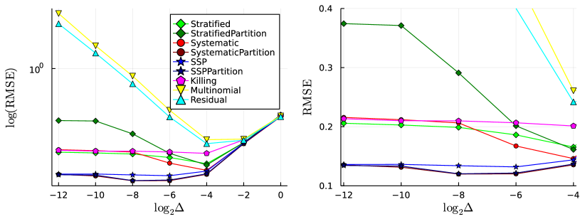
Figure 1. Normalising constant estimates with $N=512$ in the OU example. While the left panel uses a log scale and compares all the resampling schemes, the right panel uses a linear scale to compare more finely those resampling schemes that do not diverge as $\Delta\rightarrow 0$.

Figure 1 shows the normalising constant estimate mean squared errors (MSEs) in the case $N=512$. When $\Delta=2^{0}$, the performance is almost identical across resampling schemes, as we are not in the weakly informative setting, but this is no longer the case as $\Delta\to 0$. As expected, the performance of multinomial and residual resampling decay as $\Delta\to 0$, while other resampling schemes remain stable. The increase in relative RMSE for the multinomial scheme supports related results in [5] that show the variance of the normalising constant estimate increases exponentially with the number of resampling instances. Similar to multinomial, residual resampling rate does not stabilise (see comment after Assumption 2) and hence the observed variance increase as $\Delta$ decreases. The zoomed figure on the right suggests that the best performance is obtained with SystematicPartition and SSPPartition. SSP resampling is also close, and seems indistinguishable in the $\Delta\to 0$ limit.

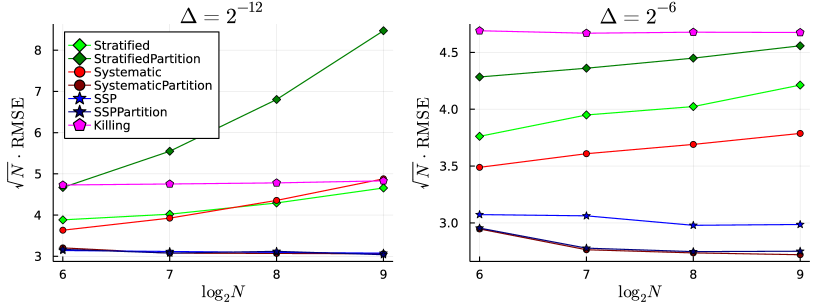
Figure 2. Normalising constant estimates with different $N$ in the OU example. Each panel corresponds to a different value of $\Delta$.

Figure 2 shows a similar picture for varying $N$, with two choices of $\Delta$. The values of the y-axis are RMSEs multiplied by $\sqrt{N}$, which is expected to stabilise if a central limit theorem type result holds. The results suggest that Killing, SSP, SSPPartition and SystematicPartition indeed stabilise, with the latter two being again the best.

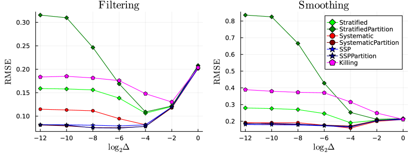
Figure 3. Filtering and smoothing estimates with $N=512$ in the OU example.

Figure 3 shows filtering and smoothing estimate MSEs for stable resampling schemes similar to Figure 1. The conclusions are similar, except for systematic resampling, which seems to be competitive with the best schemes in smoothing, but not in filtering.

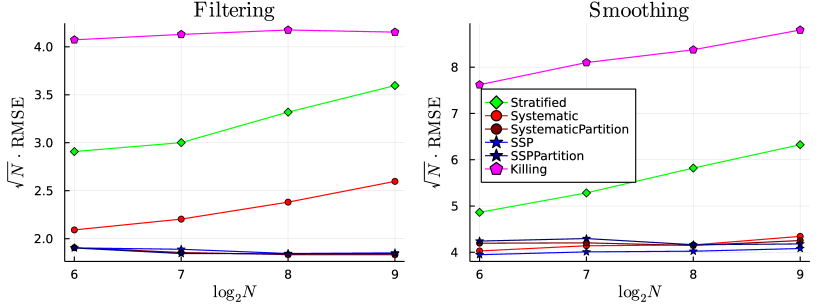
Figure 4. Filtering and smoothing estimates with $\Delta=2^{-12}$ and varying $N$ in the OU example.

Figure 4 shows filtering and smoothing estimate MSEs scaled with $\sqrt{N}$ similar to Figure 2. Again, Killing, SSP, SSPPartition and SystematicPartition seem stable in the case of filtering, but smoothing with Killing has not stabilised yet.

7.2. Comparison with adaptive resampling

Adaptive resampling [25] is a commonly used method with particle filters, where resampling is performed only when so-called effective sample size of the weights falls below a predefined threshold (fraction of particles). Adaptive resampling is out of the scope of our theoretical framework, but can be useful in practice also in the weak potentials setting, so we compare empirically how adaptive resampling performs in the OU example (Section 7.1).

Figure 5 shows the performance with adaptive resampling with $N=512$ particles and threshold $t_{\mathrm{res}}=0.5$, in the filtering and smoothing, similar to Figure 3.

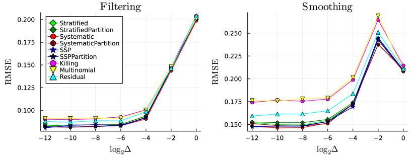
Figure 5. Adaptive resampling with threshold $0.5$ and $N=512$ in the OU example.

Adaptive resampling seems stable with all resamplings, the differences between resamplings are small, and the performance is competitive with the best non-adaptive resamplings. The behaviour with smaller number of particles is qualitatively similar to $N=512$ (results not shown).

The threshold value, which controls how often resampling is triggered, is a tuning parameter of the method. We repeated the experiment with a range of thresholds $t_{\mathrm{res}}\in\{k/8\,:\,k=0,\ldots,8\}\cup\{1-2^{-k}\,:\,k=4,\ldots,9\}$. Figure 6 shows a comparison of the results with finest discretisation $\Delta=2^{-12}$.

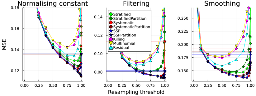
Figure 6. Adaptive resampling with $\log_{2}\Delta=-12$ and varying threshold in the OU example. The horizontal lines indicate the performance with non-adaptive resmplings ($t_{\mathrm{res}}=1.0$).

The differences between resamplings are small with low threshold values, but more noticeable with higher thresholds. For normalising constant estimation and filtering, adaptive Multinomial resampling does not reach the efficiency of the best non-adaptive schemes. In contrast, adaptive resampling can improve on the smoothing performance, and for instance with $t_{\mathrm{res}}=0.5$ all adaptive resamplings outperform the best non-adaptive resampling. Interestingly, the optimal threshold value appears to depend on the resampling. For Multinomial, Residual and Killing, the optimal value is close to $0.5$, but for SSPPartition and SystematicPartition, the optimal threshold is closer to one.

7.3. Cox process with Particle marginal Metropolis-Hastings

In our second example, we consider a Cox process model, that is, an inhomogeneous Poisson process with random intensity. We infer the latent intensity based on event times $0<\tau_{1}<\cdots<\tau_{m}<\tau$, leading to the following model:

(13) $$\Pi(\phi)\mathrel{\mathop{:}}=\frac{1}{\mathcal{Z}_{\mathbb{M}}}\mathbb{E}_{\mathbb{M}}\bigg{[}\phi\big{(}Z_{[0,\tau]}\big{)}\exp\bigg{(}-\int_{0}^{\tau}V_{u}(Z_{u})\mathrm{d}u\bigg{)}\prod_{i=1}^{m}V_{\tau_{i}}(Z_{\tau_{i}})\bigg{]},$$

where $\mathbb{M}$ stands for the law of a reflected Brownian motion on $[a,b]$, and the potential $V_{u}(z)=\beta e^{-\alpha z}$.

We approximate the reflected Brownian motion with the discrete-time dynamics $M_{1}=N(0,1)$ and $M_{k}(\cdot\mid X_{k-1})$ for $k\geq 1$:

$$\hat{X}_{k}\sim N(X_{k-1},\Delta_{k}\sigma^{2});\qquad X_{k}=\mathrm{reflect}(\hat{X}_{k};a,b),$$

where $\Delta_{k}=t_{k}-t_{k-1}$ is the time difference between $X_{k-1}$, and $X_{k}$ and $\mathrm{reflect}$ implements a folding back to $[a,b]$.

We consider synthetic data $\tau=(\tau_{1},\ldots,\tau_{n})$ generated from the model, where $Z_{t}$ is the càdlàg extension of the skeleton $Z_{t_{k}}=X_{k}$ on $[0,T]$. We use the constant step size $\Delta_{k}=\Delta=0.01$ and the parameter values $\sigma=0.3$, $\alpha=1.0$, $\beta=0.5$ and $T=200$ in the simulation.

We then use the particle marginal Metropolis-Hastings (PMMH) [1] to do posterior inference with independent $N(0,2.5)$ prior for all log-transformed parameters $\theta=(\log\sigma,\log\alpha,\log\beta)$. The discretisation mesh is a uniform grid as in the data generation, augmented with the data points. The potentials are defined as follows:

$$\log G_{k}(x)=-\Delta_{k+1}\beta\exp(-\alpha X_{k})+1(t_{k}\in\tau)(\log(\beta)-\alpha X_{k})$$

That is, the latter part is only included in case of data point is observed at $t_{k}$. The initial value of the PMMH is set to $\theta_{0}=(0,0,0)$. We use the continuous covariance adaptation scheme of [19] within PMMH [cf. 30] during the entire simulation of 500,000 iterations, with 50,000 taken as as burn-in. We repeat the experiment with $N\in\{16,32,64,128,256\}$ particles and the same range of resampling algorithms as in the previous experiment.

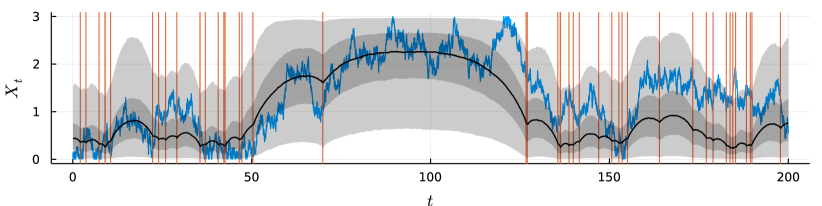
Figure 7. Generated latent state (blue) and observed times $y$ (red) in the Cox process experiment, as well as the posterior smoothing 50% and 90% credible intervals with PMMH using SystematicPartition and 32 particles.

Figure 7 shows the data in the experiment, and illustrates the inference outcome for the latent state. It is intuitive that there is substantial uncertainty in longer intervals with no observations. In these intervals, the potentials are weak, and so the resampling strategy is expected to have an impact in the efficiency.

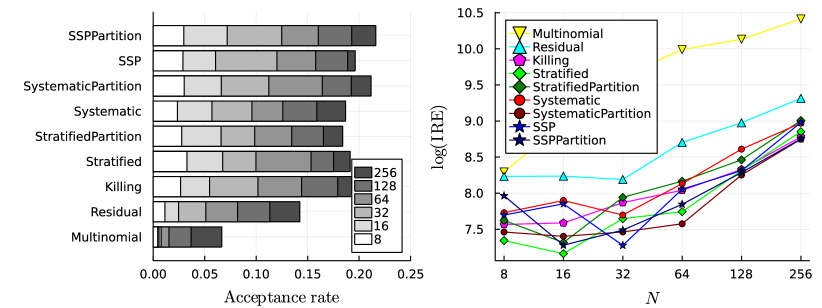
Figure 8. Acceptance rate (left) and mean inverse relative efficiency (right) of PMMH in the Cox process experiment.

Figure 8 (left) shows the PMMH acceptance rate in the different scenarios. The same group of SSP, SSPPartition and SystematicPartition attains the highest rates, and with multinomial and residual resampling, the acceptance remains notably lower. To attain a 10% acceptance rate, residual resampling needs 128 particles in contrast with 32 particles for the best resampling schemes.

Figure 8 (right) illustrates the mean inverse relative efficiencies (IREs) [17], that is, mean asymptotic variances of the standardised log-transformed parameters, multiplied by number of particles. The asymptotic variances are calculated by batch means [15], and standardisation is based on mean and variance estimates calculated from all outputs. The results are in line with earlier findings, but suggest that a low number of particles (even as low as 8) might be optimal in some cases. However, this might well be anomaly due to underestimation of asymptotic variance, which is supported by inspection of autocorrelation plots of the first parameter ($\log\alpha$) shown in Figure 9. Note that the lags are chosen inversely proportional to $N$ to account for varying cost per iteration.

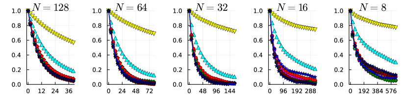
Figure 9. Autocorrelation functions of $\log\alpha$ in the Cox process experiment.

8. Discussion

We investigated the effect of resampling methods in a particle filter targeting a HMM with uninformative observations, by considering discretisations of continuous-time path integral models. We introduced a general condition for discrete-time resampling schemes which guarantees convergence to a non-degenerate particle system the continuous-time limit. We are unaware of earlier results establishing continuous-time limits of particle filters with different resampling strategies.

Resampling methods which satisfy our condition are ‘safe’ to use with weakly informative observations/potentials. We introduced modified versions of stratified/systematic/SSP resampling, which are shown to satisfy the condition. The modified strategies add a simple (and computationally cheap) algorithmic step to the resampling schemes, which orders the weights about their mean value. The modified algorithms lend themselves to a theoretical analysis, which reveals that systematic and SSP resampling schemes yield the smallest overall resampling rate, and may therefore be preferable.

Our empirical results complement our theoretical findings: systematic and SSP resampling with mean ordering had the best performance in all experiments. Because of the appealing theoretical properties of SSP resampling [cf. 16], it can be recommended also in the weakly informative regime. However, the systematic resampling may remain preferable in some settings, because of its slightly lower computational cost. Interestingly, the mean partition order, which was necessary for theoretical analysis, appears to improve the performance of systematic resampling as well. Based on our findings, we recommend that systematic resampling is always used together with the mean partition ordering of the weights. SSP resampling appears to perform well also without such pre-ordering.

Adaptive resampling [25] and further refinements, such as partial interaction schemes [32], can also be useful in the weakly informative setting, but are out of the scope of our theoretical framework. Our empirical comparison suggests that adaptive resampling can further improve performance of the studied resampling algorithms. However, optimal choice of threshold is non-trivial, as it seems to depend on the resampling scheme.

Appendix A Proofs for Section 4

We first establish results for weights that are mean partitioned and nearly constant.

Assumption 24.

Let $w^{{1:N}}$ be normalised weights and write $w^{{i}}=\frac{1+\epsilon^{{i}}}{N}$ where $\epsilon^{{i}}=Nw^{{i}}-1$. Suppose that $\sum_{i}|\epsilon^{{i}}|<2$ and that there exists $m\in[N]$ such that $\epsilon^{{1}},\ldots,\epsilon^{{m}}\leq 0$ and $\epsilon^{{m+1}},\ldots,\epsilon^{{N}}>0$.

In what follows, under Assumption 24, we denote $c^{{0}}=0$ and $c^{{i}}\mathrel{\mathop{:}}=-\sum_{j=1}^{i}\epsilon^{{j}}$ for $i\in[N]$. Then we may write the distribution function corresponding to $w^{{1:N}}$ as follows:

$$F(i)=\sum_{j=1}^{i}w^{{j}}=\frac{1}{N}\bigg{(}i-c^{i}\bigg{)}\qquad\text{for}\qquad i=0,\ldots,N.$$

Lemma 25.

Under Assumption 24:

1. $c^{{1}}\leq\cdots\leq c^{{m}}$, $c^{{m}}>\cdots>c^{{N}}$ and $c^{{i}}\in[0,1)$ for $i\in[m]$.

2. For $u\in(0,1)$ and $\check{u}^{{i}}\mathrel{\mathop{:}}=(i-1+u)/N$, the following hold:

   $$F(i-1)<\check{u}^{i}\leq F(i) \iff u\leq 1-c^{{i}}$$

   $$F(i)<\check{u}^{i}\leq F(i+1) \iff u>1-c^{{i}}.$$

Proof.

Because $\sum_{i}|\epsilon^{{i}}|=\sum_{i}(\epsilon^{{i}})_{+}+\sum_{i}(-\epsilon^{{i}})_{+}<2$, and $\sum_{i}\epsilon^{{i}}=0$ so $\sum_{i}(\epsilon^{{i}})_{+}=\sum_{i}(-\epsilon^{{i}})_{+}<1$, from which (i) follows, and (ii) is a direct consequence of $c^{i}\in[0,1)$. ∎

Lemma 26.

Let $A^{{1:N}}$ be indices from stratified resampling (Definition 6). If Assumption 24 holds, then $A^{{i}}\in\{i,i+1\}$ for all $i\in[N]$ and for any $K\subset[N-1]$ and $S=[N]\setminus K$,

$$\mathbb{P}(A^{{i}}=i,\,A^{{j}}=j+1\,\text{for all $i\in S$ and $j\in K$})=\bigg{(}\prod_{j\in S}(1-c^{{j}})\bigg{)}\bigg{(}\prod_{i\in K}c^{{i}}\bigg{)}.$$

Proof.

Because the $\check{U_{i}}$’s are independent, we may write the probability of interest as

$$\bigg{(}\prod_{j\in S}\mathbb{P}\big{(}F(j-1)<\check{U}^{{j}}\leq F(j)\big{)}\bigg{)}\bigg{(}\prod_{i\in K}\mathbb{P}\big{(}F(i)<\check{U}^{{i}}\leq F(i+1)\big{)}\bigg{)},$$

from which the result follows by Lemma 25. ∎

Lemma 27.

Let $v^{{1:N}}\geq 0$. The normalised weights $w_{\Delta}^{{1:N}}$ corresponding to unnormalised weights $g_{\Delta}^{{i}}=\exp(-\Delta v^{{i}})$ may be written as

$$w_{\Delta}^{{i}}=\frac{1+\epsilon^{{i}}_{\Delta}}{N},\qquad\text{where}\qquad\epsilon^{{i}}_{\Delta}=\Delta(\bar{v}-v^{{i}})+r_{\Delta}^{{i}}$$

where $\bar{v}=N^{-1}\sum_{i=1}^{N}v^{{i}}$ stands for the mean potential and the error terms $r_{\Delta}^{{i}}=o(\Delta)$ and satisfy $|r_{\Delta}^{{i}}|\leq c\Delta$ for all $\Delta\in(0,1)$, where the constant $c$ depends only on $N$ and $\max_{i}v^{{i}}$. Consequently,

$$c_{\Delta}^{{i}}\mathrel{\mathop{:}}=-\sum_{j=1}^{i}\epsilon_{\Delta}^{{j}}=\Delta\sum_{j=1}^{i}(v^{{j}}-\bar{v})+\tilde{r}_{\Delta}^{{i}},\qquad\tilde{r}_{\Delta}^{{i}}=o(\Delta),\qquad|\tilde{r}_{\Delta}^{{i}}|\leq\tilde{c}\Delta.$$

Proof.

Direct calculation for $\epsilon_{\Delta}^{{i}}=Ng_{\Delta}^{{i}}/\sum_{j=1}^{N}g_{\Delta}^{{j}}-1$ yields that

$$\lim_{\Delta\to 0}\frac{d}{d\Delta}\epsilon^{{i}}_{\Delta}=\frac{1}{N}\sum_{j=1}^{N}v^{{j}}-v^{{i}}=\bar{v}-v^{{i}},$$

and properties of the error term can be verified, for instance, by using a Taylor expansion for the exponential function. ∎

Proof of Proposition 9.

Suppose first that $-v^{{1:N}}$ are mean ordered, and that $\Delta$ is sufficiently small so that also $w_{\Delta}^{{1:N}}\propto\exp(-\Delta v^{{1:N}})$ satisfy Assumption 24. Lemma 27 together with Lemma 26 give

$$\lim_{\Delta\to 0+}\frac{1}{\Delta}r\big{(}a^{{1:N}}\mid\exp(-\Delta v^{{1:N}})\big{)}=\begin{cases}\sum_{j=1}^{i}(v^{{j}}-\bar{v}),&a^{{i}}=i+1$ and $a^{{\neg i}}=\neg i.\\ 0,&\text{otherwise.}\end{cases}$$

The corresponding overall resampling rate is therefore

$$\sum_{i=1}^{N}\sum_{j=1}^{i}(v^{{j}}-\bar{v})=\sum_{j=1}^{N}(N+1-j)(v^{{j}}-\bar{v})=\sum_{j=1}^{N}j(\bar{v}-v^{{j}}).$$

The claim follows from this result applied to re-indexed $v_{\varpi}$ and $a_{\varpi}$. ∎

Lemma 28.

Let $A^{{1:N}}$ be indices from systematic resampling (Definition 5). If Assumption 24 holds, then for any $k\in[m]$ and $\ell\in[N]\setminus[m]$,

$$\mathbb{P}\big{(}A^{{i}}=i\text{ for }i<k\text{ and }i\geq\ell,\;A^{{j}}=j+1\text{ for }k\leq j<\ell\big{)}$$

$$=\big{(}\min\{c^{{k}},c^{{\ell-1}}\}-\max\{c^{{k-1}},c^{{\ell}}\}\big{)}_{+},$$

and these events are the only possible in addition to the ‘no resampling’ event, for which

$$\mathbb{P}(A^{{1:N}}=1{:}N)=1-c^{{m}}.$$

Proof.

By Lemma 25, the event is equivalent to

$$\mathbb{P}\big{(}U\leq 1-c^{i}\text{ for }i<k\text{ and }i\geq\ell,\;U>1-c^{j}\text{ for }k\leq j<\ell\big{)}$$

$$=\mathbb{P}\big{(}U\in(1-c^{{k}},1-c^{{k-1}}],U\in(1-c^{{\ell-1}},1-c^{{\ell}}]\big{)},$$

thanks to the monotonicity properties of $c^{{1:m}}$ and $c^{{m+1:N}}$. The latter follows similarly because $c^{{m}}=\max_{i\in[N]}c^{{i}}$. ∎

Proof of Proposition 10.

Suppose first that $-v^{{1:N}}$ are mean ordered. Lemma 27 with Lemma 28 yield

$$\lim_{\Delta\to 0+}\frac{1}{\Delta}r\big{(}a^{{1:N}}\mid\exp(-\Delta v^{{1:N}})\big{)}=\begin{cases}\big{(}\min\{s^{{k}},s^{{\ell-1}}\}-\max\{s^{{k-1}},s^{{\ell}}\}\big{)}_{+}&a^{{1:N}}=[k\to\ell]_{N},\\ 0,&\text{otherwise},\end{cases}$$

where $s^{{0}}=0$ and $s^{{i}}=\sum_{j=1}^{i}(v^{j}-\bar{v})$. The overall resampling rate is

$$\sum_{k=1}^{m}\sum_{\ell=m+1}^{N}\big{(}\min\{s^{{k}},s^{{\ell-1}}\}-\max\{s^{{k-1}},s^{{\ell}}\}\big{)}_{+}=\sum_{k=1}^{m}(s^{{k}}-s^{{k-1}})=s^{{m}},$$

because $s^{{0:m}}$ is increasing and $s^{{m:N}}$ is decreasing. The result follows by re-indexing wrt. $\varpi$. ∎

Proposition 29.

Suppose that the normalised weights $w^{{1:N}}$ satisfy Assumption 24 and $\sum_{i=1}^{N}|\epsilon_{i}|<1$. Then, for the SSP resampling with identity order $\varpi$, the only events with non-zero probability in addition to $1{:}N$ are of the form $A^{{1:N}}=[k\to\ell]_{N}$, with probabilities:

$$\mathbb{P}(A^{{1:N}}=[k\to\ell]_{N})=\frac{(-\epsilon^{{k}})_{+}(\epsilon^{{\ell}})_{+}}{\sum_{i=1}^{N}(\epsilon^{{i}})_{+}},\qquad\text{for }k,\ell\in[N].$$

Proof.

Thanks to Assumption 24, the initial values of $p^{{1:N}}$ satisfy $p^{{i}}=1+\epsilon^{{i}}$ for $i=1,\ldots,m$ and $p^{{i}}=\epsilon^{{j}}$ for $j=m+1,\ldots,N$, and now $c^{{i}}=-\sum_{j=1}^{i}\epsilon^{{j}}\in[0,1/2)$.

Note that the state of Algorithm 2 after lines 3–4 is independent of the order of the indices $(i,j)$ before, so without loss of generality, we may assume that $i<j=k$ always before line 3. We may deduce inductively that after line 3 with $k\in\{2{:}m\}$:

• $p^{{i}}=1-c^{{k-1}}$ and $p^{{j}}=1+\epsilon^{{k}}$, and

• $p^{{i}}>1/2$ and $p^{{j}}>1/2$ and therefore $\delta^{{i}}=1-p^{{i}}=c^{{k-1}}$ and $\delta^{{j}}=1-p^{{j}}=-\epsilon^{{k}}$.

With probability $\delta^{{j}}/(\delta^{{i}}+\delta^{{j}})=-\epsilon^{{k}}/c^{{k}}$, the indices at next iteration will be $i=k$ and $j=k+1$, and $r^{1:k-1}$ have all been incremented by one. The probability to end up with indices $i=k$ and $j=m+1$ after iteration $m$ is $(-\epsilon^{{k}}/c^{{k}})\prod_{i=k+1}^{m}(c^{{i-1}}/c^{{i}})=-\epsilon^{{k}}/c^{{m}}$, in which case all $r^{{1:m}}$ have been incremented by one, except for $r^{{k}}$.

Given the above scenario happens, then in the steps $k\in\{(m+1){:}(N-1)\}$ of the algorithm, it is again easy to see inductively that $p^{{i}}+p^{{j}}=1-c^{{k}}<1$ so $\delta^{{i,j}}=p^{{j,i}}$ and that $p^{{i}}=1-c^{{j-1}}$. The probability to end up with $i=\ell$ and $j=N$ after iteration $N-1$ is therefore $\epsilon^{{\ell}}/(1-c^{{\ell}})\prod_{j=\ell+1}^{N-1}(1-c^{{j-1}})/(1-c^{{j}})=\epsilon^{{\ell}}/(1-c^{{N-1}})$, in which case in the beginning of the last step, $p^{{i}}+p^{{j}}=1-c^{{N}}=1$. Now, $r^{{\ell}}$ will be incremented by one with probability $(1-c^{{N-1}})$. We conclude the overall probability of outcome $[k\to\ell]_{N}$, which is equivalent to incrementing $r^{{\ell}}$ and $r^{{1:m}}$ by one except for $r^{{k}}$. ∎

Proof of Theorem 15.

Note that for any $i$ such that $(\bar{v}-v^{{i}})_{+}>0$, that is, $v^{{i}}<\bar{v}$, we have

$$(\bar{v}-v^{{i}})_{+}=\bar{v}-v^{{i}}\leq\bar{v}-v_{\min},$$

and there are of course at most $N-1$ such $i$, so

$$\iota_{\mathrm{systematic}}^{*}(v^{{1:N}})\leq\#\{i\,:\,v^{{i}}<\bar{v}\}(\bar{v}-v_{\min})\leq(N-1)(\bar{v}-v_{\min})=\iota_{\mathrm{killing}}^{*}(v^{{1:N}}).$$

Assuming mean ordered $-v^{{1:N}}$ we may write

$$\iota_{\mathrm{stratified}}^{*}(v^{{1:N}})-\iota_{\mathrm{systematic}}^{*}(v^{{1:N}}) =\sum_{j=1}^{m}j(\bar{v}-v^{{j}})+\sum_{j=m+1}^{N}(j-1)(\bar{v}-v^{{j}})$$

$$\geq m\sum_{j=1}^{m}(\bar{v}-v^{{j}})+m\sum_{j=m+1}^{N}(\bar{v}-v^{{j}})=0.$$

To see that there cannot be such an order between $\iota^{*}_{\mathrm{killing}}$ and $\iota^{*}_{\mathrm{stratified}}$, consider $N=3$ and strictly decreasing $v^{{1:3}}$. Now, $v_{\min}=v^{{3}}$ and

$$\iota_{\mathrm{killing}}^{*}(v^{{1:N}})-\iota_{\mathrm{stratified}}^{*}(v^{{1:N}}) =2(\bar{v}-v^{{3}})-(\bar{v}-v^{{1}})-2(\bar{v}-v^{{2}})-3(\bar{v}-v^{{3}})=v^{{2}}-\bar{v}$$

$$=\frac{2}{3}\Big{(}v^{{2}}-\frac{v^{{1}}+v^{{3}}}{2}\Big{)},$$

which can be positive or negative depending on $v^{{2}}\in(v^{{3}},v^{{1}})$. A similar example can be constructed for any $N>3$ (we omit the details). ∎

Appendix B Proof of Theorem 19

This section is dedicated to the proof of Theorem 19. Because of the technical nature of the theorem and its proof, we shall introduce some additional notation conventions specific to this section.

We use $(^{d})^{N}$ and ^dN interchangeably for the state space of the particle filters $X^{\Delta_{n}}$, $n\in\mathbb{N}$ with the following identification: for $x\in^{dN}$, write $x^{{j}}$, $j\in[N]$, for the vector $[x_{(j-1)d+1},x_{(j-1)d+2},\cdots,x_{jd-1},x_{jd}]^{\intercal}\in^{d}$, so that $x$ can be identified with $(x^{{1}},\cdots,x^{{N}})\in(^{d})^{N}$ and vice versa. In particular, superscripts ^j refer to vector components and subscripts _j to real coordinates. This distinction will mostly be clear from context in the sequel, but we will emphasise it where necessary.

B.1. A new construction of $X^{\Delta}_{k}$ in Theorem 19

For notational convenience, we present a new (equivalent) construction for the $(^{d})^{N}$-valued Markov chains $\{X^{\Delta}_{k}\}_{k\in\mathbb{N}_{0}}$ for $\Delta\in\{\Delta_{n}\,:\,n\in\mathbb{N}\}$. This new construction is self-contained in the sense that it does not make reference to Algorithm 1 (which we did when introducing this chain in Section 5).

Denote by $\mu\mathrel{\mathop{:}}=M_{1}\in\mathcal{P}(^{d})$ the initial distribution for the particles, and by $W\mathrel{\mathop{:}}=(W^{1},\cdots,W^{{N}})$ a fixed $dN$-dimensional Brownian motion (so that the $W^{{j}}$’s are independent $d$-dimensional Brownian motions) with respect to a filtration $(\mathcal{F}_{t})_{t\geq 0}$. We then redefine the Markov chain $X^{\Delta}\mathrel{\mathop{:}}=(X^{\Delta}_{k})_{k\in\mathbb{N}_{0}}$ by $(X^{\Delta}_{0})^{{j}}\sim\mu$ independently for $j\in[N]$ and

$$(X^{\Delta}_{k+1})^{{j}}=(X^{\Delta}_{k})^{{A_{k}(j)}}+b\big{(}(X^{\Delta}_{k})^{{A_{k}(j)}}\big{)}\Delta+\sigma\big{(}(X^{\Delta}_{k})^{{A_{k}(j)}}\big{)}\big{(}W^{{j}}_{(k+1)\Delta}-W^{{j}}_{k\Delta}\big{)}$$

for $k\in\mathbb{N}_{0}$ and $j\in[N]$. Here $A_{k}\in[N]^{N}$ stands for the multi-index resulting from the resampling at time $k$, i.e. $A_{k}\sim r(\cdot\mid\nu^{\Delta}(X^{\Delta}_{k}))$, and $A_{k}(j)\in[N]$ stands for the $j$’th index of $A_{k}$.

More precisely, we may write

(14) $$A_{k}=\sum_{\ell=1}^{N^{N}}\mathbf{1}\Big{(}\sum_{i=1}^{\ell-1}r(a_{i}\mid\nu^{\Delta}(X^{\Delta}_{k}))<U^{\Delta}_{k}\leq\sum_{i=1}^{\ell}r(a_{i}\mid\nu^{\Delta}(X^{\Delta}_{k}))\Big{)}a_{\ell},$$

where $\{a_{1},\cdots,a_{N^{N}}\}$ is some fixed enumeration of $[N]^{N}$, and the $U^{\Delta}_{k}$’s are uniform random variables on $(0,1)$ independent of each other and the $W^{{j}}$’s. We can take each $U^{\Delta}_{k}$ to be $\mathcal{F}_{k\Delta}$-measurable. The Markov chain $X^{\Delta}$ is then $(\mathcal{F}_{k\Delta})_{k\in\mathbb{N}_{0}}$-adapted for all $\Delta\in\{\Delta_{n}\,:\,n\in\mathbb{N}\}$.

Now define the continuous-time scaling $Z^{\Delta}$ of this Markov chain by

(15) $$Z^{\Delta}_{t}\mathrel{\mathop{:}}=X^{\Delta}_{\lfloor t/\Delta\rfloor},\quad t\in[0,\infty),$$

so that $Z^{\Delta}$ is for all $\Delta$ an $(\mathcal{F}_{t})_{t\geq 0}$-adapted process with paths in $D_{{}^{dN}}[0,\infty)$, the Skorohod space of càdlàg paths in ^dN. Recall the standard modulus of continuity of $D_{{}^{dN}}[0,\infty)$, defined for $z\in D_{{}^{dN}}[0,\infty)$, $\delta>0$ and $t>0$ by

$$\omega_{\delta,t}(z)\mathrel{\mathop{:}}=\inf_{\begin{subarray}{c}0=t_{0}<t_{1}<\cdots<t_{n-1}<t\leq t_{n}\\ t_{i}-t_{i-1}>\delta\end{subarray}}\,\max_{i\in[n]}\,\sup_{s,\,s^{\prime}\in[t_{i-1},t_{i})}|z(s^{\prime})-z(s)|.$$

B.2. Outline of the proof of Theorem 19

The main steps in the proof of parts (i) and (ii) of the theorem are as follows:

• In order to use a convergence result from [14], our first goal is to show that the family of processes $(Z^{\Delta_{n}})_{n\in\mathbb{N}}$ is relatively compact with respect to convergence in distribution, i.e. that $\{\mathbb{P}(Z^{\Delta_{n}}\in\cdot)\,:\,n\in\mathbb{N}\}$ is a relatively compact set in the weak topology of $\mathcal{P}(D_{{}^{dN}}[0,\infty))$. This is done in Proposition 30 below.

• The second step is to declare the continuous-time process $(Z_{t})_{t\geq 0}$ that the càdlàg extensions $(Z^{\Delta_{n}}_{t})_{t\geq 0}$ will converge to. The process $(Z_{t})_{t\geq 0}$ is the canonical càdlàg process $({\mathbb{X}}_{t})_{t\geq 0}$ introduced immediately before Proposition 31, equipped with a law possessing the generator ${\mathcal{L}}$. Proposition 31 proves (by establishing the well-posedness of the corresponding martingale problem) that this law is uniquely determined and Markovian.

• We then show in Proposition 32 that the appropriately-scaled discrete-time derivative of the transition kernel of $(X^{\Delta_{n}}_{k})_{k\in\mathbb{N}_{0}}$, the skeleton of $(Z^{\Delta_{n}}_{t})_{t\geq 0}$, converges in a suitable sense to the generator $\mathcal{L}$ as $n\to\infty$.

• Proposition 33 and Theorem 34 then complete the proof of parts (i) and (ii).

• The proof of part (iii) is presented in the end of the section.

B.3. The proof

Proposition 30.

The family of processes $(Z^{\Delta_{n}})_{n\in\mathbb{N}}$ satisfies

(i) the following compact containment condition:

$$\lim_{C\to\infty}\sup_{n}\mathbb{P}\big{(}|Z_{t}^{\Delta_{n}}|>C\big{)}=0$$

for every $t>0$;

(ii) the following uniform modulus of continuity condition:

$$\lim_{\delta\to 0^{+}}\sup_{n}\mathbb{P}\big{(}\omega_{\delta,t}(Z^{\Delta_{n}})>\varepsilon\big{)}=0$$

for every $t>0$ and $\varepsilon>0$.

Hence the family $(Z^{\Delta_{n}})_{n\in\mathbb{N}}$ is relatively compact with respect to convergence in distribution.

We refer to e.g. [14, Chapter 3] or [3, Chapter 3] for details on the spaces $D_{{}^{dN}}[0,\infty)$ and $\mathcal{P}(D_{{}^{dN}}[0,\infty))$. In particular, see [14, Chapter 3, Theorem 7.2] for why the conditions (i) and (ii) above together imply relative compactness. By [14, Chapter 3, Remark 7.3], relative compactness further implies the following stronger version of part (i):

(16) $$\lim_{C\to\infty}\sup_{n}\mathbb{P}\big{(}\sup_{u\in[0,t]}|Z_{u}^{\Delta_{n}}|>C\big{)}=0\quad\text{for all}\quad t>0.$$

Proof.

(i) Fix $\Delta\in(\Delta_{n})_{n\in\mathbb{N}}$. In order to avoid dealing with the jumps resulting from the resampling $r$ directly, we shall construct a larger tree of suitable discretisations of the underlying diffusion (9) which will at time $\lfloor t/\Delta\rfloor$ contain each of the $N$ particles of $X^{\Delta}_{\lfloor t/\Delta\rfloor}$ with sufficiently high probability – this will be made precise in the argument below.

Denote by $\tau_{k}$, the time indices corresponding to the resampling events of the particles $X^{\Delta}$, i.e.

$$\tau_{1}=\min\{i\geq 0\,:\,A_{i}\neq 1{:}N\}$$

and inductively

$$\tau_{k+1}=\min\{i>\tau_{k}\,:\,A_{i}\neq 1{:}N\}$$

for $k\in\mathbb{N}$. These random times are obviously stopping times with respect to the filtration $(\mathcal{F}_{k\Delta})_{k\in\mathbb{N}_{0}}$ (and well-defined with probability $1$).

For multi-indices $a$ of length $|a|=1$, i.e. $a=(j)$ for $j\in[N]$, define the Markov chains $Y^{(j)}_{k}$ in ^d by

$$Y^{(j)}_{0}=(X^{\Delta}_{0})^{{j}}\quad\textrm{and}\quad Y^{(j)}_{k+1}=Y^{(j)}_{k}+b(Y^{(j)}_{k})\Delta+\sigma(Y^{(j)}_{k})\big{(}W^{{j}}_{(k+1)\Delta}-W^{{j}}_{k\Delta}\big{)},$$

so that $Y^{(j)}_{k}=(X^{\Delta}_{k})^{{j}}$ for $k\leq\tau_{1}$, and write

$$\mathcal{Y}^{1}\mathrel{\mathop{:}}=\bigl{\{}(Y^{a}_{k})_{k\geq 0}\,:\,|a|=1\bigr{\}}$$

We then inductively define the trees $\mathcal{Y}^{\ell+1}\mathrel{\mathop{:}}=\{(Y^{a}_{k})_{k\geq 0}\,:\,|a|=\ell+1\}$ for integers $\ell>0$ by

$$Y^{a}_{k}=\begin{cases}Y^{(a(1),\cdots,a(\ell))}_{k}\quad\text{for }k\leq\tau_{\ell},\\ Y^{a}_{k-1}+b(Y^{a}_{k-1})\Delta+\sigma(Y^{a}_{k-1})\big{(}W^{{a(\ell+1)}}_{k\Delta}-W^{{a(\ell+1)}}_{(k-1)\Delta}\big{)}\quad\text{for }k>\tau_{\ell};\end{cases}$$

note in particular that for $Y^{a}\in\mathcal{Y}^{\ell+1}$, the states $Y^{(a(1),\cdots,a(\ell))}_{k}$ in the definition above come from $Y^{(a(1),\cdots,a(\ell))}\in\mathcal{Y}^{\ell}$. In other words, at time $\tau_{\ell}$ the chains in $\mathcal{Y}^{\ell}$ each branch into $N$ chains in $\mathcal{Y}^{\ell+1}$, evolving from time $\tau_{\ell}$ independently as Euler-Maruyama discretisations of the diffusion (9) driven by the $N$ Brownian motions driving the particles $(X^{\Delta})^{1:N}$.

It is then easy to see from the construction that if there have been less than $\ell$ resampling events of the particles before time $\lfloor t/\Delta\rfloor$, i.e.

$$\sum_{k=0}^{\lfloor t/\Delta\rfloor-1}\mathbf{1}\big{(}A_{k}\neq 1{:}N\big{)}<\ell,$$

then $(X^{\Delta}_{\lfloor t/\Delta\rfloor})^{{j}}\in\{Y^{a}_{\lfloor t/\Delta\rfloor}\,:\,|a|=\ell\}$ for all $j\in[N]$, so that

(17) $$|Z_{t}^{\Delta}|\leq N\sum_{|a|=\ell}|Y^{a}_{\lfloor t/\Delta\rfloor}|\leq c(\ell,N)\sqrt{\sum_{|a|=\ell}\big{(}|Y^{a}_{\lfloor t/\Delta\rfloor}-Y^{a}_{0}|^{2}+|Y^{a}_{0}|^{2}\big{)}},$$

with some constant $c(\ell,N)<\infty$ independent of $t$ and $\Delta$. On the other hand, the probability of at least $\ell$ resampling events before time $\lfloor t/\Delta\rfloor$ can be controlled independently of $\Delta$ as follows:

$$\mathbb{P}\Big{(}\sum_{k=0}^{\lfloor t/\Delta\rfloor-1}\mathbf{1}\big{(}A_{k}\neq 1{:}N\big{)}\geq\ell\Big{)} \leq\frac{1}{\ell}\sum_{k=0}^{\lfloor t/\Delta\rfloor-1}\mathbb{P}\big{(}A_{k}\neq 1{:}N\big{)}$$

(18) $$\leq\frac{1}{\ell}\sum_{k=0}^{\lfloor t/\Delta\rfloor-1}(c^{\prime}\Delta)\leq\frac{c^{\prime}t}{\ell},$$

where the constant $c^{\prime}$ is independent of $\Delta$, $t$ and $\ell$ (see (8) and (14)). Combining (17) and (18) thus yields

$$\mathbb{P}(|Z_{t}^{\Delta}|>C) \leq\mathbb{P}\Big{(}\sum_{|a|=\ell}\big{(}|Y^{a}_{\lfloor t/\Delta\rfloor}-Y^{a}_{0}|^{2}+|Y^{a}_{0}|^{2}\big{)}>\frac{C^{2}}{c(\ell,N)^{2}}\Big{)}+\frac{c^{\prime}t}{\ell}$$

$$\leq\mathbb{P}\Big{(}\sum_{|a|=\ell}|Y^{a}_{\lfloor t/\Delta\rfloor}-Y^{a}_{0}|^{2}>\frac{C^{2}}{2c(\ell,N)^{2}}\Big{)}+\mathbb{P}\Big{(}\sum_{|a|=\ell}|Y^{a}_{0}|^{2}>\frac{C^{2}}{2c(\ell,N)^{2}}\Big{)}+\frac{c^{\prime}t}{\ell}$$

$$\leq\frac{2c(\ell,N)^{2}}{C^{2}}\sum_{|a|=\ell}\mathbb{E}\big{[}|Y^{a}_{\lfloor t/\Delta\rfloor}-Y^{a}_{0}|^{2}\big{]}+\mathbb{P}\Big{(}\sum_{|a|=\ell}|Y^{a}_{0}|^{2}>\frac{C^{2}}{2c(\ell,N)^{2}}\Big{)}+\frac{c^{\prime}t}{\ell}.$$

Now the term $c^{\prime}t/\ell$ can be made arbitrarily small by a choice of $\ell$ independent of $\Delta$, and for fixed $\ell$ the term

$$\mathbb{P}\Big{(}\sum_{|a|=\ell}|Y^{a}_{0}|^{2}>\frac{C^{2}}{2c(\ell,N)^{2}}\Big{)}$$

obviously converges to zero as $C\to\infty$ uniformly in $\Delta$ (since each $Y^{a}_{0}$ is distributed as the initial distribution $\mu$). In other words, (i) follows if we can obtain an estimate for each $\mathbb{E}[|Y^{a}_{\lfloor t/\Delta\rfloor}-Y^{a}_{0}|^{2}]$ which may depend on $|a|=\ell$ and $t$ but not on $\Delta$.

To this end, note that the tree construction implies that

$$Y^{a}_{\lfloor t/\Delta\rfloor}-Y^{a}_{0} =\sum_{k=1}^{\lfloor t/\Delta\rfloor}\big{(}Y^{a}_{k}-Y^{a}_{k-1}\big{)}=\sum_{k=1}^{\lfloor t/\Delta\rfloor}\Big{(}b(Y^{a}_{k-1})\Delta+\sigma(Y^{a}_{k-1})\big{(}W^{{j^{a}_{k-1}}}_{k\Delta}-W^{{j^{a}_{k-1}}}_{(k-1)\Delta}\big{)}\Big{)}$$

(19) $$=\sum_{k=1}^{\lfloor t/\Delta\rfloor}b(Y^{a}_{k-1})\Delta+\sum_{k=1}^{\lfloor t/\Delta\rfloor}\sigma(Y^{a}_{k-1})\big{(}W^{{j^{a}_{k-1}}}_{k\Delta}-W^{{j^{a}_{k-1}}}_{(k-1)\Delta}\big{)},$$

where each $j^{a}_{k}$ is an $\mathcal{F}_{k\Delta}$-measurable random index. Since $b$ is bounded, we simply get

$$\mathbb{E}\Big{[}\big{|}\sum_{k=1}^{\lfloor t/\Delta\rfloor}b(Y^{a}_{k-1})\Delta\big{|}^{2}\Big{]}\leq\big{(}\lfloor t/\Delta\rfloor\|b\|_{L^{\infty}}\Delta]\big{)}^{2}\leq\|b\|_{L^{\infty}}^{2}t^{2}.$$

For the latter sum in (19), note that

(20) $$\sigma(Y^{a}_{k-1})\big{(}W^{{j^{a}_{k-1}}}_{k\Delta}-W^{{j^{a}_{k-1}}}_{(k-1)\Delta}\big{)}=\sum_{j\in[N]}\mathbf{1}\big{(}j^{a}_{k-1}=j\big{)}\sigma(Y^{a}_{k-1})\big{(}W^{{j}}_{k\Delta}-W^{{j}}_{(k-1)\Delta}\big{)},$$

where the terms $\mathbf{1}(j^{a}_{k-1}=j)$ and $\sigma(Y^{a}_{k-1})$ are $\mathcal{F}_{(k-1)\Delta}$-measurable and the terms $W^{{j}}_{k\Delta}-W^{{j}}_{(k-1)\Delta}$ are distributed as $\mathcal{N}(0,\Delta I_{{}^{d}})$ independently of $\mathcal{F}_{(k-1)\Delta}$, so it is fairly easy to see that each real component of the ^d-valued Markov chain

$$n\mapsto\sum_{k=1}^{n}\sigma(Y^{a}_{k-1})\big{(}W^{{j^{a}_{k-1}}}_{k\Delta}-W^{{j^{a}_{k-1}}}_{(k-1)\Delta}\big{)}$$

is a martingale, which leads to the estimate

$$\mathbb{E}\Big{[}\big{|}\sum_{k=1}^{\lfloor t/\Delta\rfloor}\sigma(Y^{a}_{k-1})\big{(}W^{{j^{a}_{k-1}}}_{k\Delta}-W^{{j^{a}_{k-1}}}_{(k-1)\Delta}\big{)}\big{|}^{2}\Big{]}$$

$$\qquad\qquad=\sum_{k=1}^{\lfloor t/\Delta\rfloor}\mathbb{E}\Big{[}\big{|}\sigma(Y^{a}_{k-1})\big{(}W^{{j^{a}_{k-1}}}_{k\Delta}-W^{{j^{a}_{k-1}}}_{(k-1)\Delta}\big{)}\big{|}^{2}\Big{]}$$

$$\qquad\qquad\leq\|\sigma\|_{L^{\infty}}^{2}\sum_{k=1}^{\lfloor t/\Delta\rfloor}\mathbb{E}\Big{[}\sum_{j\in[N]}\mathbf{1}\big{(}j^{a}_{k-1}=j\big{)}\big{|}W^{{j}}_{k\Delta}-W^{{j}}_{(k-1)\Delta}\big{|}^{2}\Big{]}$$

$$\qquad\qquad=\|\sigma\|_{L^{\infty}}^{2}\sum_{k=1}^{\lfloor t/\Delta\rfloor}\sum_{j\in[N]}\mathbb{E}\Big{[}\mathbf{1}\big{(}j^{a}_{k-1}=j\big{)}\mathbb{E}\big{[}\big{|}W^{{j}}_{k\Delta}-W^{{j}}_{(k-1)\Delta}\big{|}^{2}\big{|}\mathcal{F}_{(k-1)\Delta}\big{]}\Big{]}$$

$$\qquad\qquad=\|\sigma\|_{L^{\infty}}^{2}\lfloor t/\Delta\rfloor\Delta\leq\|\sigma\|_{L^{\infty}}^{2}t.$$

This finishes the proof of (i).

(ii) Fix $t>0$, $\varepsilon>0$ and $\gamma>0$, with $\gamma$ arbitrarily small. We will show that

(21) $$\limsup_{\delta\to 0^{+}}\Big{(}\sup_{\Delta\in(\Delta_{n})_{n\in\mathbb{N}}}\mathbb{P}\big{(}\omega_{\delta,t}(Z^{\Delta})>\varepsilon\big{)}\Big{)}\leq\gamma,$$

which by the arbitrariness of $\gamma>0$ implies (ii).

Consider parameters $0<\Delta\leq\delta\ll 1$ (since obviously $\omega_{\delta,t}(Z^{\Delta^{\prime}})\equiv 0$ for $\Delta^{\prime}>\delta$), where the condition “$\ll 1$” is quantified more precisely later on. Like in (18) above, it will be convenient to disregard the possibility of arbitrarily many resampling events of the Markov chain $X^{\Delta}$ before the time $\lfloor t/\Delta\rfloor$:

$$\mathbb{P}\Big{(}\sum_{k=0}^{\lfloor t/\Delta\rfloor-1}\mathbf{1}\big{(}A_{k}\neq 1{:}N\big{)}\geq\ell\Big{)}\leq\frac{c^{\prime}t}{\ell},$$

and $\ell\in\mathbb{N}$ can be taken so that the latter quantity is $<\gamma$. We can further limit our estimates to the case when the resampling events up to time $\tau_{\ell}$ happen happen sufficiently sparsely. Denoting $\tau_{0}\equiv 0$, we have

$$\mathbb{P}(\tau_{k}-\tau_{k-1}\leq m) =\sum_{n}\mathbb{P}(\tau_{k}\leq m+n\mid\tau_{k-1}=n)\mathbb{P}(\tau_{k-1}=n)$$

$$=\sum_{n}\mathbb{P}\Big{(}\sum_{i=n+1}^{n+m}\mathbf{1}\big{(}A_{i}\neq 1{:}N\big{)}\geq 1\mid\tau_{k-1}=n\Big{)}\mathbb{P}(\tau_{k-1}=n)$$

$$\leq\sum_{n}c^{\prime}\Delta m\mathbb{P}(\tau_{k-1}=n)=c^{\prime}\Delta m$$

for any $k$, $m\in\mathbb{N}$, and so

$$\mathbb{P}\Big{(}\bigcup_{k=1}^{\ell}\{\tau_{k}-\tau_{k-1}\leq\lfloor 2\delta/\Delta\rfloor\}\Big{)}\leq 2\ell c^{\prime}\delta.$$

Thus the event

(22) $$B\mathrel{\mathop{:}}=\Big{\{}\sum_{k=0}^{\lfloor t/\Delta\rfloor-1}\mathbf{1}\big{(}A_{k}\neq 1{:}N\big{)}<\ell\Big{\}}\cap\bigcap_{k=1}^{\ell}\{\tau_{k}-\tau_{k-1}>\lfloor 2\delta/\Delta\rfloor\}$$

has probability

(23) $$\mathbb{P}(B)\geq 1-\gamma-2\ell c^{\prime}\delta,$$

which is sufficiently high for our purposes.

Now consider $\omega_{\delta,t}(Z^{\Delta})$ within the event $B$. Denote by $\tau^{*}$ the smallest resampling time $\tau_{k}$ such that $\tau_{k}\geq\lfloor t/\Delta\rfloor$. By (22) we have $\tau^{*}\leq\tau_{\ell}$ and $(\tau_{k}-\tau_{k-1})\Delta>\lfloor 2\delta/\Delta\rfloor\Delta>\delta$ for $\tau_{k}\leq\tau^{*}$. Obviously $(\tau^{*}+1)\Delta\geq t$. Thus the partition

(24) $$0<(\tau_{1}+1)\Delta<(\tau_{2}+1)\Delta<\cdots<(\tau^{*}+1)\Delta$$

is a valid candidate for the infimum in the definition of $\omega_{\delta,t}$. However since some of the interval lengths $(\tau_{k}-\tau_{k-1})\Delta$ may be unnecessarily long for estimating $\omega_{\delta,t}(Z^{\Delta})$, we shall refine the partition (24) as follows. Let

$$0=t_{0}<t_{1}<\cdots<t_{m-1}<t\leq t_{m}$$

be such that $\{(\tau_{k}+1)\Delta\,:\,\tau_{k}<\tau^{*}\}\subset\{t_{i}\,:\,i<m\}$, $t_{i}-t_{i-1}\in(\delta,2\delta]$ and $t_{m}\leq\min((\tau^{*}+1)\Delta,t+2\delta)$. To see why this is possible, simply divide any interval of the form $[(\tau_{k-1}+1)\Delta,(\tau_{k}+1)\Delta)$ with length $>2\delta$ into sufficiently many smaller subintervals.

Note that we do not claim that the path-wise choice of the partition $\{t_{i}\}$ in $B$ is in any way measurable, but this will ultimately not be an issue below. The partition will be used as a stepping stone for a path-wise upper bound for $\omega_{\delta,t}(Z^{\Delta})$ (for paths in $B$) which is measurable.

The point of the above construction is that jumps induced by the resampling will not happen on continuous-time intervals of the type $[t_{i-1},t_{i})$, as is easily seen from the original partition (24). Thus

$$\omega_{\delta,t}(Z^{\Delta}) \leq\max_{i\in[m]}\,\sup_{s,\,s^{\prime}\in[t_{i-1},t_{i})}|Z^{\Delta}_{s^{\prime}}-Z^{\Delta}_{s}|=\max_{i\in[m]}\,\max_{\lfloor\frac{t_{i-1}}{\Delta}\rfloor\leq k,\,k^{\prime}<\lfloor\frac{t_{i}}{\Delta}\rfloor}|X^{\Delta}_{k^{\prime}}-X^{\Delta}_{k}|$$

$$\leq\sum_{j\in[N]}\max_{i\in[m]}\,\max_{\lfloor\frac{t_{i-1}}{\Delta}\rfloor\leq k,\,k^{\prime}<\lfloor\frac{t_{i}}{\Delta}\rfloor}|(X^{\Delta}_{k^{\prime}})^{{j}}-(X^{\Delta}_{k})^{{j}}|$$

$$=\sum_{j\in[N]}\max_{i\in[m]}\,\max_{\lfloor\frac{t_{i-1}}{\Delta}\rfloor\leq k<k^{\prime}<\lfloor\frac{t_{i}}{\Delta}\rfloor}\big{|}\sum_{k\leq i<k^{\prime}}b((X^{\Delta}_{i})^{{j}})\Delta+\sum_{k\leq i<k^{\prime}}\sigma((X^{\Delta}_{i})^{{j}})\big{(}W^{{j}}_{(i+1)\Delta}-W^{{j}}_{i\Delta}\big{)}\big{|}.$$

The first inner sum can be estimated as follows:

$$\big{|}\sum_{k\leq i<k^{\prime}}b((X^{\Delta}_{i})^{{j}})\Delta\big{|} \leq(k^{\prime}-k)\|b\|_{L^{\infty}}\Delta\leq\|b\|_{L^{\infty}}\Big{(}\Big{\lfloor}\frac{t_{i}}{\Delta}\Big{\rfloor}-\Big{\lfloor}\frac{t_{i-1}}{\Delta}\Big{\rfloor}\Big{)}\Delta$$

$$\leq\|b\|_{L^{\infty}}\Big{(}\frac{t_{i}}{\Delta}-\frac{t_{i-1}}{\Delta}+1\Big{)}\Delta\leq 3\|b\|_{L^{\infty}}\delta,$$

and here we specify the assumption (already implicitly made above) that $\delta<\varepsilon/(6N\|b\|_{L^{\infty}})$. Applying this estimate to the one above yields

$$\omega_{\delta,t}(Z^{\Delta})\leq\frac{\varepsilon}{2}+\sum_{j\in[N]}\max_{i\in[m]}\,\max_{\lfloor\frac{t_{i-1}}{\Delta}\rfloor\leq k<k^{\prime}<\lfloor\frac{t_{i}}{\Delta}\rfloor}\big{|}\sum_{k\leq i<k^{\prime}}\sigma((X^{\Delta}_{i})^{{j}})\big{(}W^{{j}}_{(i+1)\Delta}-W^{{j}}_{i\Delta}\big{)}\big{|}.$$

To sidestep the measurability issues arising from the path-wise choice of the partition $\{t_{i}\}$, note that for any $i\in[m]$ we can find $n\in\{0,\cdots,\lceil t/\delta\rceil\}$ such that

$$\Big{\{}\Big{\lfloor}\frac{t_{i-1}}{{\Delta}}\Big{\rfloor},\Big{\lfloor}\frac{t_{i-1}}{\Delta}\Big{\rfloor}+1,\cdots,\Big{\lfloor}\frac{t_{i}}{\Delta}\Big{\rfloor}-1\Big{\}}\subset\Big{\{}n\Big{\lceil}\frac{\delta}{\Delta}\Big{\rceil},n\Big{\lceil}\frac{\delta}{\Delta}\Big{\rceil}+1,\cdots,(n+3)\Big{\lceil}\frac{\delta}{\Delta}\Big{\rceil}-1\Big{\}},$$

so

$$\omega_{\delta,t}(Z^{\Delta}) \leq\frac{\varepsilon}{2}+\sum_{j\in[N]}\max_{0\leq n\leq\lceil\frac{t}{\delta}\rceil}\,\,\max_{n\lceil\frac{\delta}{\Delta}\rceil\leq k<k^{\prime}<(n+3)\lceil\frac{\delta}{\Delta}\rceil}\big{|}\sum_{k\leq i<k^{\prime}}\sigma((X^{\Delta}_{i})^{{j}})\big{(}W^{{j}}_{(i+1)\Delta}-W^{{j}}_{i\Delta}\big{)}\big{|}$$

$$\leq\frac{\varepsilon}{2}+2\sum_{j\in[N]}\max_{0\leq n\leq\lceil\frac{t}{\delta}\rceil}\,\,\underbrace{\max_{n\lceil\frac{\delta}{\Delta}\rceil<k<(n+3)\lceil\frac{\delta}{\Delta}\rceil}\big{|}\sum_{n\lceil\frac{\delta}{\Delta}\rceil\leq i<k}\sigma((X^{\Delta}_{i})^{{j}})\big{(}W^{{j}}_{(i+1)\Delta}-W^{{j}}_{i\Delta}\big{)}\big{|}}_{=:M^{{j}}_{n}}.$$

Combining this with (22) and (23) thus yields

$$\mathbb{P}\big{(}\omega_{\delta,t}(Z^{\Delta})>\varepsilon\big{)} \leq\mathbb{P}\Big{(}\frac{\varepsilon}{2}+2\sum_{j\in[N]}\max_{0\leq n\leq\lceil\frac{t}{\delta}\rceil}M^{{j}}_{n}>\varepsilon\Big{)}+2\ell c^{\prime}\delta+\gamma$$

$$\leq\sum_{j\in[N]}\mathbb{P}\Big{(}\max_{0\leq n\leq\lceil\frac{t}{\delta}\rceil}M^{{j}}_{n}>\frac{\varepsilon}{4N}\Big{)}+2\ell c^{\prime}\delta+\gamma$$

(25) $$\leq\sum_{j\in[N]}\sum_{0\leq n\leq\lceil t/\delta\rceil}\mathbb{P}\Big{(}M^{{j}}_{n}>\frac{\varepsilon}{4N}\Big{)}+2\ell c^{\prime}\delta+\gamma.$$

Then in order to estimate a term of the form $\mathbb{P}(M^{{j}}_{n}>\frac{\varepsilon}{4N})$, recall from the discussion following (20) that each real component of the ^d-valued Markov chain

$$k\mapsto S^{{j}}_{n,k}\mathrel{\mathop{:}}=\sum_{n\lceil\frac{\delta}{\Delta}\rceil\leq i<k}\sigma((X^{\Delta}_{i})^{{j}})\big{(}W^{{j}}_{(i+1)\Delta}-W^{{j}}_{i\Delta}\big{)},\qquad k\geq n\Big{\lceil}\frac{\delta}{\Delta}\Big{\rceil},$$

is a martingale starting from zero (i.e. the sum above is interpreted as zero for $k=n\lceil\delta/\Delta\rceil$). Write $[S^{{j}}_{n}]_{k}$ for

$$\sum_{n\lceil\frac{\delta}{\Delta}\rceil\leq i<k}\big{|}\sigma((X^{\Delta}_{i})^{{j}})\big{(}W^{{j}}_{(i+1)\Delta}-W^{{j}}_{i\Delta}\big{)}\big{|}^{2},$$

which is the sum of the quadratic variations of the real components of $S^{{j}}_{n,\cdot}$ up to time $k>n\lceil\delta/\Delta\rceil$. Then, for arbitrary fixed $p>2$, we may use the Burkholder-Davis-Gundy inequality (see e.g. [29, pp. 499] or [24, Theorem 18.7]) and Hölder’s inequality to obtain

$$\mathbb{P}\Big{(}M^{{j}}_{n}>\frac{\varepsilon}{4N}\Big{)} \lesssim\varepsilon^{-p}\mathbb{E}\big{[}|M^{{j}}_{n}|^{p}\big{]}\lesssim\varepsilon^{-p}\mathbb{E}\big{[}[S^{{j}}_{n}]_{(n+3)\lceil\frac{\delta}{\Delta}\rceil}^{p/2}\big{]}$$

$$\lesssim\varepsilon^{-p}\mathbb{E}\Big{[}\Big{(}\sum_{n\lceil\frac{\delta}{\Delta}\rceil\leq i<(n+3)\lceil\frac{\delta}{\Delta}\rceil}\big{|}\sigma((X^{\Delta}_{i})^{{j}})\big{(}W^{{j}}_{(i+1)\Delta}-W^{{j}}_{i\Delta}\big{)}\big{|}^{2}\Big{)}^{p/2}\Big{]}$$

$$\lesssim\varepsilon^{-p}\|\sigma\|_{L^{\infty}}^{p}\Big{\lceil}\frac{\delta}{\Delta}\Big{\rceil}^{(p-2)/2}\mathbb{E}\Big{[}\sum_{n\lceil\frac{\delta}{\Delta}\rceil\leq i<(n+3)\lceil\frac{\delta}{\Delta}\rceil}\big{|}W^{{j}}_{(i+1)\Delta}-W^{{j}}_{i\Delta}\big{|}^{p}\Big{]}$$

$$\lesssim\varepsilon^{-p}\|\sigma\|_{L^{\infty}}^{p}\Big{\lceil}\frac{\delta}{\Delta}\Big{\rceil}^{p/2}\Delta^{p/2}\lesssim\varepsilon^{-p}\|\sigma\|_{L^{\infty}}^{p}\delta^{p/2},$$

where the implicit multiplicative constant in each inequality is independent of $\delta$ and $\Delta$ (but can of course depend on $p$, $N$ and the dimension $d$ of the state space of the particles). Applying this estimate to (25) gives

$$\mathbb{P}\big{(}\omega_{\delta,t}(Z^{\Delta})>\varepsilon\big{)}\leq c^{\prime\prime}t\varepsilon^{-p}\|\sigma\|_{L^{\infty}}^{p}\delta^{(p/2)-1}+2\ell c^{\prime}\delta+\gamma$$

with constants $c^{\prime}$ and $c^{\prime\prime}$ independent of $\delta$ and $\Delta$, and since $(p/2)-1>0$, this yields (21) and thus finishes the proof of (ii). ∎

Our next step is to verify that the infinitesimal generator ${\mathcal{L}}$ in Theorem 19 is associated with a well-posed martingale problem. Let us briefly recall the concept of martingale problems.

Denote by ${\mathbb{X}}$ the canonical càdlàg process, given by the projections

$$D_{{}^{dN}}[0,\infty)\owns z\mapsto{\mathbb{X}}_{t}(z)\mathrel{\mathop{:}}=z(t)\in^{dN},$$

and by ${\mathbb{F}}$ the filtration generated by ${\mathbb{X}}$. The martingale problem for $({\mathcal{L}},C^{\infty}_{c}(^{dN}))$ concerns the existence of a probability measure $\mathbb{P}_{\eta}\in\mathcal{P}(D_{{}^{dN}}[0,\infty))$ for any given $\eta\in\mathcal{P}(^{dN})$ such that

$$(t,z)\mapsto f({\mathbb{X}}_{t}(z))-f({\mathbb{X}}_{0}(z))-\int_{0}^{t}{\mathcal{L}}f({\mathbb{X}}_{u}(z))\mathrm{d}u$$

is a martingale (with respect to ${\mathbb{F}}$) under $\mathbb{P}_{\eta}$ for any $f\in C^{\infty}_{c}(^{dN})$, and $\mathbb{P}_{\eta}\circ({\mathbb{X}}_{0})^{-1}=\eta$. The martingale problem is said to be well-posed if for every $\eta$ a solution $\mathbb{P}_{\eta}$ exists and is unique. To be more precise, “uniqueness” here means uniqueness in terms of finite-dimensional distributions – we refer to [14, Chapter 4] for a thorough examination of this subject.

In order to write the generator ${\mathcal{L}}$ explicitly, we slightly abuse notation and define the functions $b^{*}\colon^{dN}\to^{dN}$ and $\sigma^{*}\colon^{dN}\to^{dN}\times^{dN}$ for $x\mathrel{\mathop{:}}=(x^{{1}},x^{{2}},\cdots,x^{{N}})\in(^{d})^{N}$ by

$$b_{i}^{*}(x)=\big{(}b(x^{{j}})\big{)}_{i-(j-1)d}\qquad\text{for}\qquad j\in[N]\text{ and }(j-1)d<i\leq jd$$

and

$$\sigma^{*}_{i,j}(x)=\begin{cases}\big{(}\sigma(x^{{k}})\big{)}_{i-(k-1)d,j-(k-1)d}\quad&\text{if}\quad(k-1)d<i,\,j\leq kd\text{ for some }k\in[N],\\ 0&\text{otherwise}.\end{cases}$$

Recall that the subscripts _i are to be interpreted as real coordinates ^d or ^dN, the subscripts _i,j as real entries of a matrix in ${}^{d}\times^{d}$ or ${}^{dN}\times^{dN}$ and the superscripts ^j as ^d-components of $(^{d})^{N}$, keeping in line with our previous notation. The functions $b^{*}$ and $\sigma^{*}$ obviously have the same properties $b$ and $\sigma$, i.e. they are Lipschitz continuous and bounded, and $\sigma^{*}$ is uniformly non-degenerate in the sense of (10).

We then have

$${\mathcal{L}}f(x) =\Big{(}\sum_{i=1}^{dN}b^{*}_{i}(x)\partial_{i}f(x)+\frac{1}{2}\sum_{i,j=1}^{dN}\big{(}\sigma^{*}(x)^{\intercal}\sigma^{*}(x)\big{)}_{i,j}\partial_{i,j}f(x)\Big{)}$$

$$\quad\qquad\qquad+\sum_{a\in[N]^{N}\setminus\{1{:}N\}}\iota^{a}(x)\big{(}f(x^{{a(1{:}N)}})-f(x)\big{)}$$

(26) $$=:{\mathcal{L}}^{\textrm{mut}}f(x)+{\mathcal{L}}^{\textrm{jump}}f(x)$$

for $f\in C^{\infty}_{c}(^{dN})$, where the jump intensity functions $\iota^{a}\colon^{dN}\to[0,\infty)$ were assumed to be bounded and continuous. Recall that $x^{{a(1{:}N)}}$ above stands for $(x^{{a(1)}},\cdots,x^{{a(N)}})$.

Proposition 31.

The martingale problem for $({\mathcal{L}},C^{\infty}_{c}(^{dN}))$ is well-posed.

Proof.

Write $C^{\infty}_{c}\mathrel{\mathop{:}}=C^{\infty}_{c}(^{dN})$. A fairly general existence result by W. Hoh, see [22, Theorem 3.15] or [4, Theorem 3.24] and the references therein, implies that the martingale problem for $({\mathcal{L}},C^{\infty}_{c})$ with our assumptions for the coefficient functions has a solution for any initial distribution $\eta$.

In order to verify uniqueness, we first note that our assumptions on the coefficient functions $b^{*}$ and $\sigma^{*}$ imply that ${\mathcal{L}}^{\textrm{mut}}$ is a standard non-degenerate (in the sense of (10)) diffusion-type generator, so the martingale problem for $({\mathcal{L}}^{\textrm{mut}},C^{\infty}_{c})$ is well-posed, and in fact ${\mathcal{L}}^{\textrm{mut}}$ generates a Feller process – see e.g. [14, Chapter 8, Section 1] and [24, Theorem 17.24].

Then consider cutoff functions $\chi^{k}\in C^{\infty}_{c}$, $k\in\mathbb{N}$, such that $0\leq\chi^{k}\leq 1$ and $\chi^{k}(x)=1$ for $|x|\leq k$. A standard perturbation result implies that each ${\mathcal{L}}^{k}\mathrel{\mathop{:}}={\mathcal{L}}^{\textrm{mut}}+\chi^{k}{\mathcal{L}}^{\textrm{jump}}$, i.e.

$${\mathcal{L}}^{k}f(x)={\mathcal{L}}^{\textrm{mut}}f(x)+\chi^{k}(x)\sum_{a\in[N]^{N}\setminus\{1{:}N\}}\iota^{a}(x)\big{(}f(x^{{a(1{:}N)}})-f(x)\big{)},$$

is a Feller generator and that well-posedness holds for the martingale problem for $({\mathcal{L}}^{k},C^{\infty}_{c})$; see e.g. [14, Chapter 1, Theorem 7.1] or [23, Theorem 2.8.1]. The cutoff function $\chi^{k}$ is needed here to ensure that ${\mathcal{L}}^{k}$ maps functions in $C^{\infty}_{c}$ to continuous functions that vanish at infinity, which is not necessarily the case for ${\mathcal{L}}$ itself since the jump intensity functions $\iota^{a}$ are merely continuous and bounded.

Finally, since the martingale problem for $({\mathcal{L}},C^{\infty}_{c})$ has a solution for any initial distribution as noted above, and ${\mathcal{L}}$ always coincides locally with some ${\mathcal{L}}^{k}$, a standard localisation procedure for the well-posedness of martingale problems [14, Chapter 4, Theorems 6.1 and 6.2] yields well-posedness for the martingale problem for $({\mathcal{L}},C^{\infty}_{c})$. ∎

Finally, let us check that appropriately-scaled discrete generators of the Markov chains $X^{\Delta_{n}}$ converge to ${\mathcal{L}}$.

Proposition 32.

For $n\in\mathbb{N}$, write $\Gamma_{n}$ for the transition kernel of $X^{\Delta_{n}}$. Then

$${\mathcal{L}}_{n}f(x)\mathrel{\mathop{:}}=\frac{1}{\Delta_{n}}\Big{(}\int_{{}^{dN}}f(y)\Gamma_{n}(x,\mathrm{d}y)-f(x)\Big{)}\stackrel{{\scriptstyle n\to\infty}}{{\longrightarrow}}{\mathcal{L}}f(x)$$

for all $f\in C^{\infty}_{c}(^{dN})$ with bounded and pointwise convergence with respect to $x\in^{dN}$, i.e. ${\mathcal{L}}_{n}f$ is uniformly bounded for all $f$.

Proof.

Let $\Delta\mathrel{\mathop{:}}=\Delta_{n}$ for some $n$. With the notation introduced above, we have

$$X^{\Delta}_{k+1} =\sum_{a\in[N]^{N}}\mathbf{1}\big{(}A_{k}=a\big{)}\Big{(}(X^{\Delta}_{k})^{{a(1{:}N)}}+b^{*}\big{(}(X^{\Delta}_{k})^{{a(1{:}N)}}\big{)}\Delta$$

$$\qquad\qquad+\sigma^{*}\big{(}(X^{\Delta}_{k})^{{a(1{:}N)}}\big{)}(W_{(k+1)\Delta}-W_{k\Delta})\Big{)},$$

where $W_{t}\mathrel{\mathop{:}}=(W^{1}_{t},\cdots,W^{N}_{t})$. Thus, $\Gamma_{n}$ can be expressed as

$$\int_{{}^{dN}}f(y)\Gamma_{n}(x,\mathrm{d}y)=\mathbb{E}\Big{[}\sum_{a\in[N]^{N}}\mathbf{1}\big{(}A^{\Delta}(x)=a\big{)}f\big{(}x^{{a(1{:}N)}}+b^{*}(x^{{a(1{:}N)}})\Delta+\sigma^{*}(x^{{a(1{:}N)}})B^{\Delta}\big{)}\Big{]}$$

for $x\in^{dN}$ and bounded and Borel measurable $f\colon^{dN}\to$, where

$$A^{\Delta}(x)=\sum_{\ell=1}^{N^{N}}\mathbf{1}\Big{(}\sum_{i=1}^{\ell-1}r(a_{i}\mid\nu^{\Delta}(x))<U\leq\sum_{i=1}^{\ell}r(a_{i}\mid\nu^{\Delta}(x))\Big{)}a_{\ell}$$

for some $U\sim\mathcal{U}(0,1)$ and $B^{\Delta}\sim\mathcal{N}(0,\Delta I_{{}^{dN}})$ independent from $U$.

A standard application of Taylor’s theorem then justifies the following calculations for $f\in C^{\infty}_{c}(^{dN})$:

$$\int_{{}^{dN}}f(y)\Gamma_{n}(x,\mathrm{d}y)-f(x)$$

$$\quad=\int_{{}^{dN}}\big{(}f(y)-f(x)\big{)}\Gamma_{n}(x,\mathrm{d}y)$$

$$\quad=\sum_{a\in[N]^{N}}\mathbb{E}\Big{[}\mathbf{1}\big{(}A^{\Delta}(x)=a\big{)}\big{(}f\big{(}x^{{a(1{:}N)}}+b^{*}(x^{{a(1{:}N)}})\Delta$$

$$\qquad\qquad\qquad+\sigma^{*}(x^{{a(1{:}N)}})B^{\Delta}\big{)}-f(x)\big{)}\Big{]}$$

$$\quad=r\big{(}1{:}N\mid\nu^{\Delta}(x)\big{)}\big{(}{\mathcal{L}}^{\textrm{mut}}f(x)\Delta+o(\Delta)\big{)}$$

(27) $$\qquad\qquad\qquad+\sum_{a\in[N]^{N}\setminus\{1{:}N\}}r(a|\nu^{\Delta}(x))\big{(}f(x^{{a(1{:}N)}})-f(x)+O(\Delta)\big{)}.$$

To be more precise, note that if $a=a_{\ell}$, then within the event $\{A^{\Delta}(x)=a\}$ the term

$$f\big{(}x^{{a(1{:}N)}}+b^{*}(x^{{a(1{:}N)}})\Delta+\sigma^{*}(x^{{a(1{:}N)}})B^{\Delta}\big{)}$$

can be estimated by a sufficiently regular sum of terms of the form $g(x^{{a(1{:}N)}})h(B^{\Delta}),$ and

$$\mathbb{E}\Big{[}\mathbf{1}\big{(}A^{\Delta}(x)=a\big{)}g(x^{{a(1{:}N)}})h(B^{\Delta})\Big{]}$$

$$\quad=g(x^{{a(1{:}N)}})\mathbb{E}\Big{[}\mathbf{1}\Big{(}\sum_{i=1}^{\ell-1}r(a_{i}\mid\nu^{\Delta}(x))<U\leq\sum_{i=1}^{\ell}r(a_{i}\mid\nu^{\Delta}(x))\Big{)}h(B^{\Delta})\Big{]}$$

$$\quad=g(x^{{a(1{:}N)}})\mathbb{E}\Big{[}\mathbf{1}\Big{(}\sum_{i=1}^{\ell-1}r(a_{i}\mid\nu^{\Delta}(x))<U\leq\sum_{i=1}^{\ell}r(a_{i}\mid\nu^{\Delta}(x))\Big{)}\Big{]}\mathbb{E}[h(B^{\Delta})]$$

$$\quad=g(x^{{a(1{:}N)}})r(a\mid\nu^{\Delta}(x))\mathbb{E}[h(B^{\Delta})]$$

for each such term, and so the calculations and estimates for each multi-index can be carried out as one would when computing the generator a standard diffusion process.

In particular, from (27) and the assumption (8) we get

$$\lim_{n\to\infty}\frac{1}{\Delta_{n}}\Big{(}\int_{{}^{dN}}f(y)\Gamma_{n}(x,\mathrm{d}y)-f(x)\Big{)}={\mathcal{L}}^{\textrm{mut}}f(x)+{\mathcal{L}}^{\textrm{jump}}f(x)={\mathcal{L}}f(x),$$

with bounded and pointwise convergence with respect to $x$. ∎

From the last three auxiliary results we obtain

Proposition 33.

Let $Z$ be the solution to the martingale problem for $({\mathcal{L}},C^{\infty}_{c}(^{dN}))$ with initial distribution

$$\mu\times\mu\times\cdots\times\mu\in\mathcal{P}(^{dN})$$

(see Proposition 31). Then

$$\lim_{n\to\infty}Z^{\Delta_{n}}=Z$$

in distribution, i.e.

$$\lim_{n\to\infty}\mathbb{E}[F(Z^{\Delta_{n}})]=\mathbb{E}[F(Z)]$$

for all bounded and continuous $F\colon D_{{}^{dN}}[0,\infty)\to$.

Proof.

We aim to apply [14, Corollary 8.13, Chapter 4], which requires us to verify a number of conditions. The notation for the auxiliary processes below, $\xi^{f}_{n}$ and $\varphi^{f}_{n}$, follows closely the statement of said result.

Recall first that the family $(Z^{\Delta_{n}})_{n\in\mathbb{N}}$ is relatively compact in the sense of Proposition 30, and that the function space $C^{\infty}_{c}(^{dN})$ is separating in the sense that for $P$, $Q\in\mathcal{P}(^{dN})$,

$$\int f\,\mathrm{d}P=\int f\,\mathrm{d}Q\quad\forall f\in C^{\infty}_{c}(^{dN})$$

implies $P=Q$. For $f\in C^{\infty}_{c}(^{dN})$ and $t\geq 0$, write $\xi^{f}_{n}(t)\mathrel{\mathop{:}}=f(Z^{\Delta_{n}}_{t})$ and $\varphi^{f}_{n}(t)\mathrel{\mathop{:}}={\mathcal{L}}_{n}f(Z^{\Delta_{n}}_{t})$. Then we obviously have

$$\sup_{n}\sup_{s\leq t}\mathbb{E}[|\xi^{f}_{n}(s)|]<\infty\qquad\text{and}\qquad\sup_{n}\sup_{s\leq t}\mathbb{E}[|\varphi^{f}_{n}(s)|]<\infty$$

for all $f\in C^{\infty}_{c}(^{dN})$ and $t>0$,

$$\lim_{n\to\infty}\mathbb{E}\Big{[}\big{(}\xi^{f}_{n}(t)-f(Z^{\Delta_{n}}_{t})\big{)}\prod_{i=1}^{k}h_{i}\big{(}Z^{\Delta_{n}}_{t_{i}}\big{)}\Big{]}=0$$

for all $f\in C^{\infty}_{c}(^{dN})$, $\{h_{1},\cdots,h_{k}\}\subset C^{\infty}_{c}(^{dN})$ and $0\leq t_{1}<\cdots<t_{k}\leq t$ (trivially by the definition of $\xi^{f}_{n}$), and

$$\lim_{n\to\infty}\mathbb{E}\Big{[}\big{(}\varphi^{f}_{n}(t)-{\mathcal{L}}f(Z^{\Delta_{n}}_{t})\big{)}\prod_{i=1}^{k}h_{i}\big{(}Z^{\Delta_{n}}_{t_{i}}\big{)}\Big{]}=0$$

for $f$, $h_{i}$ and $t_{i}$ like above by dominated convergence via the bounded and pointwise convergence of the ${\mathcal{L}}_{n}f^{\prime}s$ (see Proposition 32). Thus [14, Corollary 8.13, Chapter 4] implies the desired convergence. ∎

Theorem 19 still does not automatically follow from this, since functions of finite-dimensional distributions are in general not continuous on $D_{{}^{dN}}[0,\infty)$. Let us thus formulate the following convergence result which essentially encapsulates the three parts of Theorem 19.

Theorem 34.

Let $Z$ be the càdlàg process in Proposition 33. Then

(28) $$\lim_{n\to\infty}\mathbb{E}[f(Z^{\Delta_{n}}_{t_{1}},\cdots,Z^{\Delta_{n}}_{t_{T}})F(Z^{\Delta_{n}})]=\mathbb{E}[f(Z_{t_{1}},\cdots,Z_{t_{T}})F(Z)]$$

for all finite $\{t_{1},\cdots,t_{T}\}\subset[0,\infty)$ and bounded and continuous functions $f\colon(^{dN})^{T}\to$ and $F\colon D_{{}^{dN}}[0,\infty)\to$.

Proof.

We first establish (28) with the additional assumption that $f$ is Lipschitz continuous. To this end, note that first that

$$z\mapsto\frac{1}{\delta}\int_{0}^{\delta}f(z_{t_{1}+h},\cdots,z_{t_{T}+h})dh\cdot F(z)=:Q^{\delta}(z)$$

is for any $\delta>0$ a continuous function on the Skorohod space $D_{{}^{dN}}[0,\infty)$, and by the càdlàg property

$$\lim_{\delta\to 0^{+}}Q^{\delta}(z)=f(z_{t_{1}},\cdots,z_{t_{T}})F(z)=:Q(z)$$

with bounded and pointwise convergence with respect to $z\in D_{{}^{dN}}[0,\infty)$. Thus,

$$|\mathbb{E}[Q(Z)]-\mathbb{E}[Q(Z^{\Delta_{n}})]|\leq |\mathbb{E}[Q(Z)-Q^{\delta}(Z)]|+|\mathbb{E}[Q^{\delta}(Z)-Q^{\delta}(Z^{\Delta_{n}})]|$$

(29) $$\qquad+|\mathbb{E}[Q^{\delta}(Z^{\Delta_{n}})-Q(Z^{\Delta_{n}})]|.$$

By the dominated convergence theorem, the first term on the right-hand side of (29) can be taken arbitrarily small by considering any sufficiently small $\delta>0$. For a fixed $\delta>0$, the second term is arbitrarily small for small enough $\Delta_{n}\in(0,\delta)$ by the convergence in distribution of the processes. For the third term, note that

$$|\mathbb{E}[Q^{\delta}(Z^{\Delta_{n}})-Q(Z^{\Delta_{n}})]| \leq c_{F}\mathbb{E}\Big{[}\frac{1}{\delta}\int_{0}^{\delta}|f(Z^{\Delta_{n}}_{t_{1}+h},\cdots,Z^{\Delta_{n}}_{t_{T}+h})-f(Z^{\Delta_{n}}_{t_{1}},\cdots,Z^{\Delta_{n}}_{t_{T}})|dh\Big{]}$$

$$\leq c_{f,F}\sum_{i=1}^{T}\mathbb{E}\big{[}\sup_{t_{i}<s<t_{i}+\delta}|Z^{\Delta_{n}}_{s}-Z^{\Delta_{n}}_{t}|\land 1\big{]}$$

$$\leq c_{f,F}\sum_{i=1}^{T}\Big{(}\mathbb{E}\big{[}\sup_{t_{i}<s<t_{i}+\delta}|Z^{\Delta_{n}}_{s}-Z^{\Delta_{n}}_{t}|^{2}\land 1\big{]}\Big{)}^{1/2}.$$

The expectation in the $i$th term above can be estimated by

$$\mathbb{E}\Big{[}\max_{\lfloor\frac{t_{i}}{\Delta_{n}}\rfloor<k\leq\lfloor\frac{t_{i}+\delta}{\Delta_{n}}\rfloor}|X^{\Delta_{n}}_{k}-X^{\Delta_{n}}_{\lfloor t_{i}/\Delta_{n}\rfloor}|^{2}\land 1\Big{]},$$

and we may estimate the latter quantity uniformly in $\Delta_{n}<\delta$ in a familiar manner: the probability of any resampling-induced jumps of $X^{\Delta_{n}}$ between the indices in the inner maximum is at most of order $\delta$, and outside of this event, the term

$$\max_{\lfloor\frac{t_{i}}{\Delta_{n}}\rfloor<k\leq\lfloor\frac{t_{i}+\delta}{\Delta_{n}}\rfloor}|X^{\Delta_{n}}_{k}-X^{\Delta_{n}}_{\lfloor t_{i}/\Delta_{n}\rfloor}|^{2}$$

can be estimated using a martingale decomposition and the Burkholder-Davis-Gundy inequality (with $p=2$ for the sake of simplicity) like in the proof part (ii) of Proposition 30, resulting in an upper bound of order $\delta$.

This finishes the proof of (28) for bounded and Lipschitz continuous $f$. The convergence then extends to bounded and uniformly continuous $f$ by a standard $\varepsilon/3$-argument, since any such function can be approximated uniformly by Lipschitz continuous functions.

Finally, if $f\colon(^{dN})^{T}\to$ is a bounded and continuous function, the compact containment condition (part (i) of Proposition 30) implies that there is a compact set $K\subset(^{dN})^{T}$ such that $(Z^{\Delta_{n}}_{t_{1}},\cdots,Z^{\Delta_{n}}_{t_{T}})\in K$ and $(Z_{t_{1}},\cdots,Z_{t_{T}})\in K$ with probability arbitrarily close to $1$. Subsequently there is a uniformly continuous $g\colon(^{dN})^{T}\to$ such that $g\equiv f$ on $K$ and $\|g\|_{L^{\infty}}\leq\|f\|_{L^{\infty}}$. Thus an $\varepsilon/3$-argument again establishes (28) for $f$. ∎

Proof of Theorem 19.

Parts (i) and (ii) follow automatically by taking $F\equiv 1$ in Theorem 34 above.

For part (iii), note first that for fixed $\tau>0$ the function

$$D_{{}^{dN}}[0,\infty)\owns z\mapsto F(z)\mathrel{\mathop{:}}=\exp\big{(}-\int_{0}^{\tau}\mathcal{V}(u,z_{u})\mathrm{d}u\big{)}$$

is continuous, so

(30) $$\lim_{n\to\infty}\mathbb{E}[f(Z^{\Delta_{n}}_{\tau})F(Z^{\Delta_{n}})]=\mathbb{E}[f(Z_{\tau})F(Z)]$$

by Theorem 34. On the other hand, using the simple estimate $|e^{-x}-e^{-y}|\leq|x-y|\land 1$ for $x$, $y\geq 0$, we can estimate

$$\Big{|}\mathbb{E}[f(Z^{\Delta_{n}}_{\tau})F(Z^{\Delta_{n}})]-\mathbb{E}\Big{[}f(X^{\Delta_{n}}_{\lfloor\tau/\Delta_{n}\rfloor})\prod_{k=0}^{\lfloor\tau/\Delta_{n}\rfloor-1}e^{-\Delta_{n}\mathcal{V}(k\Delta_{n},X^{\Delta_{n}}_{k})}\Big{]}\Big{|}$$

$$\qquad=\mathbb{E}\Big{[}|f(Z^{\Delta_{n}}_{\tau})|\big{|}F(Z^{\Delta_{n}})-\exp\big{(}-\Delta_{n}\sum_{k=0}^{\lfloor\tau/\Delta_{n}\rfloor-1}\mathcal{V}(k\Delta_{n},Z^{\Delta_{n}}_{k\Delta_{n}}\big{)}\big{|}\Big{]}$$

(31) $$\qquad\leq\|f\|_{L^{\infty}}\mathbb{E}\Big{[}\big{|}\int_{0}^{\tau}\mathcal{V}(u,Z^{\Delta_{n}}_{u})\mathrm{d}u-\Delta_{n}\sum_{k=0}^{\lfloor\tau/\Delta_{n}\rfloor-1}\mathcal{V}(k\Delta_{n},Z^{\Delta_{n}}_{k\Delta_{n}})\big{|}\land 1\Big{]}.$$

Now since $\mathcal{V}$ is uniformly continuous on compact subsets of $[0,\infty)\times^{dN}$ and the paths $(Z^{\Delta_{n}}_{u})_{0\leq u\leq\tau}$ stay inside some compact subset of ^dN with arbitrarily high probability (see the discussion after the statement of Proposition 30, in particular (16)), it is fairly easy to see that (31) converges to zero as $n\to\infty$. Combining this with (30) above yields the desired convergence. ∎

Appendix C Proof of Theorem 22

We start with the following auxiliary result, which states the intuitively simple fact that although the sample paths of the particle filter $Z$ are discontinuous with probability $1$, the probability of discontinuities (i.e. resampling-induced jumps) at any given time is negligible.

Proposition 35.

Let $Z$ be the càdlàg process in Theorem 19. Then

$$\mathbb{P}\big{(}Z_{t}=Z_{t-}\big{)}=1$$

for all $t>0$.

Proof.

We only give a brief outline of a proof. It suffices to show that

(32) $$\mathbb{E}\big{[}|f(Z_{t})-f(Z_{t-})|\big{]}=0$$

for any bounded and Lipschitz continuous $f\colon^{dN}\to$. The càdlàg property implies that

$$f(z_{t})-f(z_{t-})=\lim_{\delta\to 0^{+}}\frac{1}{\delta}\Big{(}\int_{t}^{t+\delta}f(z_{u})\mathrm{d}u-\int_{t-\delta}^{t}f(z_{u})\mathrm{d}u\Big{)}$$

for all $z\in D_{{}^{dN}}[0,\infty)$ and $t>0$ with bounded and pointwise convergence, and the expression inside the limit is for each $\delta>0$ a continuous function of $z\in D_{{}^{dN}}[0,\infty)$. We can then proceed as in the proof of Theorem 34, noting that resampling-induced jumps of the processes $Z^{\Delta_{n}}$ happen with arbitrarily small probability on arbitrarily small time intervals. ∎

Proof of Theorem 22.

It suffices to establish (12) for $f\in C^{\infty}_{c}(^{d})$, since any bounded and measurable function on ^d can be approximated pointwise by an uniformly bounded sequence of functions in $C^{\infty}_{c}(^{d})$.

Write

$${\mathcal{Q}}_{t}(F)\mathrel{\mathop{:}}=\mathbb{E}\Big{[}F(Z_{t})\exp\Big{(}-\int_{0}^{t}\overline{V}(Z_{u})\mathrm{d}u\Big{)}\Big{]}$$

for $F\in C^{\infty}_{c}(^{dN})$ and

$$Q_{t}(f)\mathrel{\mathop{:}}=\mathbb{E}\Big{[}f(z_{t})\exp\Big{(}-\int_{0}^{t}V(z_{u})\mathrm{d}u\Big{)}\Big{]}$$

for $f\in C^{\infty}_{c}(^{d})$.

For fixed $F$, the measure flow ${\mathcal{Q}}_{t}(F)$ is differentiable with respect to $t>0$. In order to show this and compute $\frac{\mathrm{d}}{\mathrm{d}t}{\mathcal{Q}}_{t}(F)$, write $E_{t}\mathrel{\mathop{:}}=\exp(-\int_{0}^{t}\overline{V}(Z_{u})\mathrm{d}u)$ for $t>0$. Then for $\delta>0$ with $\delta\ll 1$,

$$F(Z_{t+\delta})E_{t+\delta}-F(Z_{t})E_{t}=E_{t}\big{(}F(Z_{t+\delta})-F(Z_{t})\big{)}+F(Z_{t+\delta})\big{(}E_{t+\delta}-E_{t}\big{)}.$$

By the martingale problem (see Appendix B), $F(Z_{t+\delta})-F(Z_{t})$ can be written as $M_{t+\delta}-M_{t}+\int_{t}^{t+\delta}{\mathcal{L}}F(Z_{u})\mathrm{d}u$ for some martingale $M$ (with respect to the filtration $\mathcal{F}^{Z}$ generated by $Z$). Using this in combination with the tower property of conditional expectations (with respect to $\mathcal{F}^{Z}_{t}$), we can calculate

$${\mathcal{Q}}_{t+\delta}(F)-{\mathcal{Q}}_{t}(F)=\mathbb{E}\Big{[}E_{t}\int_{t}^{t+\delta}{\mathcal{L}}F(Z_{u})\mathrm{d}u\Big{]}+\mathbb{E}\big{[}F(Z_{t+\delta})\big{(}E_{t+\delta}-E_{t}\big{)}\big{]}.$$

The càdlàg property in conjunction with the dominated convergence theorem then implies

$$\lim_{\delta\to 0^{+}}\frac{{\mathcal{Q}}_{t+\delta}(F)-{\mathcal{Q}}_{t}(F)}{\delta}=\mathbb{E}[{\mathcal{L}}F(Z_{t})E_{t}]-\mathbb{E}[F(Z_{t})\overline{V}(Z_{t})E_{t}]={\mathcal{Q}}_{t}\big{(}({\mathcal{L}}-\overline{V})F\big{)}.$$

For negative $\delta$, we may compute ${\mathcal{Q}}_{t+\delta}(F)-{\mathcal{Q}}_{t}(F)$ in a similar manner by using the tower property with respect to the filtration $\mathcal{F}^{Z}_{t+\delta}$ instead of $\mathcal{F}^{Z}_{t}$. Then Proposition 35 above together with the dominated convergence theorem imply

(33) $$\lim_{\delta\to 0^{-}}\frac{{\mathcal{Q}}_{t+\delta}(F)-{\mathcal{Q}}_{t}(F)}{\delta}={\mathcal{Q}}_{t}\big{(}({\mathcal{L}}-\overline{V})F\big{)}.$$

In a similar (in fact easier since the sample paths of $z$ are automatically continuous) way we may calculate

(34) $$\frac{\mathrm{d}}{\mathrm{d}t}Q_{t}(f)=Q_{t}\big{(}(L-V)f\big{)}$$

for any $f\in C^{\infty}_{c}(^{d})$, where $L$ is the infinitesimal generator corresponding to the diffusion (9).

Now the left-hand side of the statement of the Theorem is ${\mathcal{Q}}_{t}(\overline{f})=:\hat{Q}_{t}(f)$ and the right-hand side is $Q_{t}(f)$. We will show that the evolution equation for $\hat{Q}$ is of the same form as (34). To this end, recall that ${\mathcal{L}}={\mathcal{L}}^{\textrm{mut}}+{\mathcal{L}}^{\textrm{jump}}$ as in (26). For $f\in C^{\infty}_{c}(^{d})$, we simply get ${\mathcal{L}}^{\textrm{mut}}(\overline{f})=\overline{Lf}$, and further

$${\mathcal{L}}^{\textrm{jump}}(\overline{f})(x) =\sum_{a\neq 1{:}N}\iota^{a}(x)\Big{(}\frac{1}{N}\sum_{i=1}^{N}f(x^{{a(i)}})-\frac{1}{N}\sum_{i=1}^{N}f(x^{{i}})\Big{)}$$

$$=\frac{1}{N}\sum_{i=1}^{N}\Big{(}\sum_{a\neq 1{:}N}\iota^{a}(x)(\#_{a,i}-1)\Big{)}f(x^{{i}}),$$

where $\#_{a,i}\mathrel{\mathop{:}}=\#\{j\,:\,a(j)=i\}$. Thus, comparing the right-hand sides of (33) and (34) (with $\overline{f}$ in place of $F$), we see that

$$\frac{\mathrm{d}}{\mathrm{d}t}\hat{Q}_{t}(f)=\hat{Q}_{t}\big{(}(L-V)f\big{)}$$

is equivalent to

(35) $${\mathcal{Q}}_{t}\Big{(}\frac{1}{N}\sum_{i=1}^{N}\Big{(}\sum_{a\neq 1{:}N}\iota^{a}(x)(\#_{a,i}-1)\Big{)}f(x^{{i}})\Big{)}={\mathcal{Q}}_{t}(\overline{V}\cdot\overline{f}-\overline{Vf}).$$

Writing out the expression inside the right-hand side parentheses and comparing the coefficients of the $f(x^{{i}})$’s, one sees that (35) will follow from the identity

(36) $$\sum_{a\neq 1{:}N}\iota^{a}(x)(\#_{a,i}-1)=\overline{V}(x)-V(x^{{i}})$$

for all $i$ and $x$, which is simply assumption (i) of the Theorem.

Thus the measure flows $Q$ and $\hat{Q}$ satisfy the same evolution equation, and by the assumptions we have $Q_{0}=\hat{Q}_{0}$. Our next task is to verify that this evolution equation is well-posed in a suitable sense.

In order to work in a space of probability measures, let us denote by $\dot{}^{d}$ the standard one-point compactification of ^d with infinity point $o$. Define the probability measures $Q_{t}^{o}\in\mathcal{P}(\dot{}^{d})$ and $\hat{Q}_{t}^{o}\in\mathcal{P}(\dot{}^{d})$, $t\geq 0$, by

$$Q_{t}^{o}(f)\mathrel{\mathop{:}}=Q_{t}(f_{|^{d}})+\big{(}1-Q_{t}(1_{|^{d}})\big{)}f(o)=Q_{t}\big{(}(f-f(o))_{|^{d}}\big{)}+f(o)$$

for (bounded and) continuous $f\colon\dot{}^{d}\to$ and similarly for $\hat{Q}$ in place of $Q$. Define $M$ as the collection of continuous functions $f$ on $\dot{}^{d}$ such that

$$\big{(}f-f(o)\big{)}_{|^{d}}\in C^{\infty}_{c}(^{d}),$$

and define the linear operator $A$ on $M$ by

$$Af(x)=L\big{(}f-f(o)\big{)}_{|^{d}}(x)+V(x)\big{(}f(o)-f(x)\big{)},\quad x\in\dot{}^{d},$$

with the understanding that $Af(o)=0$.

Now the flows $Q^{o}$ and $\hat{Q}^{o}$ both satisfy the forward equation

(37) $$\mu_{t}(f)=\mu_{0}(f)+\int_{0}^{t}\mu_{u}(Af)\mathrm{d}u,\quad t>0,$$

for (the natural extensions of) $f\in C^{\infty}_{c}(^{d})$, and it is easy to see that this extends to $f\in M$. We are thus in a place to apply a uniqueness result from [14]: it is routinely verified that $A$ satisfies the positive maximum principle, $M$ is an algebra of functions that is dense in the space of continuous functions on $\dot{}^{d}$ (with respect to the $\sup$-norm), and the $D_{\dot{}^{d}}[0,\infty)$-martingale problem for $(A,M)$ is well-posed (see Appendix B). Thus [14, Chapter 4, Proposition 9.19] yields well-posedness for the forward equation (37).

In particular, $Q^{o}_{t}(f)=\hat{Q}^{o}_{t}(f)$ for all $t>0$ and (extensions of) $f\in C^{\infty}_{c}(^{d})$, which translates to $Q_{t}(f)=\hat{Q}_{t}(f)$. ∎

Finally, let us prove Proposition 23:

Proof of Proposition 23.

Let $i\in[N]$, $v^{{1{:}N}}\in[0,\infty)^{N}$ and $\Delta>0$. By Assumption 1,

$$\frac{Ne^{-\Delta v^{{i}}}}{\sum_{j=1}^{N}e^{-\Delta v^{{j}}}} =\sum_{j=1}^{N}r\big{(}a(j)=i\mid\exp(-\Delta v^{{1{:}N}})\big{)}=\sum_{j=1}^{N}\sum_{a\in[N]^{N}}r\big{(}a\mid\exp(-\Delta v^{{1{:}N}})\big{)}\mathbf{1}\left(a(j)=i\right)$$

$$=\sum_{a\in[N]^{N}}r\big{(}a\mid\exp(-\Delta v^{{1{:}N}})\big{)}\#\{j\,:\,a(j)=i\},$$

and subtracting $\sum_{a\in[N]^{N}}r(a\mid\exp(-\Delta v^{{1{:}N}}))\equiv 1$ from this yields

$$\sum_{a\neq 1{:}N}r\big{(}a\mid\exp(-\Delta v^{{1{:}N}})\big{)}\big{(}\#\{j\,:\,a(j)=i\}-1\big{)}=\frac{Ne^{-\Delta v^{{i}}}-\sum_{j=1}^{N}e^{-\Delta v^{{j}}}}{\sum_{j=1}^{N}e^{-\Delta v^{{j}}}}.$$

Dividing this by $\Delta$ and taking $\Delta\to 0^{+}$ leads to (11), as in the proof of Lemma 27. ∎

Supplementary material

Source codes for the experiments are available at https://github.com/mvihola/weakly-informative-resampling-codes

References

• Andrieu et al. [2010] C. Andrieu, A. Doucet, and R. Holenstein. Particle Markov chain Monte Carlo methods. J. R. Stat. Soc. Ser. B Stat. Methodol., 72(3):269–342, 2010.
• Arnaudon and Del Moral [2020] M. Arnaudon and P. Del Moral. A duality formula and a particle Gibbs sampler for continuous time Feynman-Kac measures on path spaces. Electron. J. Probab., 25:Paper No. 157, 54, 2020. doi: 10.1214/20-ejp546.
• Billingsley [1999] P. Billingsley. Convergence of probability measures. John Wiley & Sons, Inc., New York, 2nd edition, 1999.
• Böttcher et al. [2013] B. Böttcher, R. Schilling, and J. Wang. Lévy Matters III. Lévy-type processes: construction, approximation and sample path properties. Springer, Cham, 2013.
• Cérou et al. [2011] F. Cérou, P. D. Moral, and A. Guyader. A nonasymptotic theorem for unnormalized Feynman–Kac particle models. Annales de l’Institut Henri Poincaré, Probabilités et Statistiques, 47(3):629 – 649, 2011.
• Chopin and Papaspiliopoulos [2020] N. Chopin and O. Papaspiliopoulos. An introduction to sequential Monte Carlo. Springer Series in Statistics. Springer, Cham, 2020.
• Crisan et al. [1999] D. Crisan, P. Del Moral, and T. Lyons. Discrete filtering using branching and interacting particle systems. Markov Process. Related Fields, 5(3):293–318, 1999. ISSN 1024-2953.
• Del Moral [2004] P. Del Moral. Feynman-Kac Formulae. Springer, 2004.
• Del Moral [2013] P. Del Moral. Mean field simulation for Monte Carlo integration. Chapman and Hall/CRC, 2013.
• Del Moral and Miclo [2000a] P. Del Moral and L. Miclo. A Moran particle system approximation of Feynman–Kac formulae. Stoch. Proc. Appl., 86(2):193–216, 2000a.
• Del Moral and Miclo [2000b] P. Del Moral and L. Miclo. Branching and interacting particle systems approximations of feynman-kac formulae with applications to non-linear filtering. In Séminaire de probabilités XXXIV, pages 1–145. Springer, 2000b.
• Del Moral et al. [2013] P. Del Moral, P. E. Jacob, A. Lee, L. Murray, and G. W. Peters. Feynman-Kac particle integration with geometric interacting jumps. Stoch. Anal. Appl., 31(5):830–871, 2013. ISSN 0736-2994. doi: 10.1080/07362994.2013.817247.
• Douc and Cappé [2005] R. Douc and O. Cappé. Comparison of resampling schemes for particle filtering. In Proc. ISPA 2005, pages 64–69, 2005.
• Ethier and Kurtz [1986] S. Ethier and T. Kurtz. Markov processes. Characterization and convergence. John Wiley & Sons, Inc., New York, 1986.
• Flegal and Jones [2010] J. M. Flegal and G. L. Jones. Batch means and spectral variance estimators in Markov chain Monte Carlo. Ann. Statist., 38(2):1034–1070, 2010.
• Gerber et al. [2019] M. Gerber, N. Chopin, and N. Whiteley. Negative association, ordering and convergence of resampling methods. Ann. Statist., 47(4):2236–2260, 2019.
• Glynn and Whitt [1992] P. W. Glynn and W. Whitt. The asymptotic efficiency of simulation estimators. Oper. Res., 40(3):505–520, 1992.
• Gordon et al. [1993] N. J. Gordon, D. J. Salmond, and A. F. M. Smith. Novel approach to nonlinear/non-Gaussian Bayesian state estimation. IEE Proceedings-F, 140(2):107–113, 1993.
• Haario et al. [2001] H. Haario, E. Saksman, and J. Tamminen. An adaptive Metropolis algorithm. Bernoulli, 7(2):223–242, 2001.
• Higuchi [1997] T. Higuchi. Monte Carlo filter using the genetic algorithm operators. J. Statist. Comput. Simulation, 59(1):1–23, 1997. ISSN 0094-9655.
• Hoare [1962] C. A. Hoare. Quicksort. The Computer Journal, 5(1):10–16, 1962.
• Hoh [1998] W. Hoh. Pseudo differential operators generating Markov processes. Habilitationsschrift Universität Bielefeld, Bielefeld, 1998.
• Jacob [2002] N. Jacob. Pseudo differential operators & Markov processes. Volume II: Generators and their potential theory. Imperial College Press, London, 2002.
• Kallenberg [2002] O. Kallenberg. Foundations of modern probability. Springer-Verlag, New York, 2002.
• Liu and Chen [1995] J. S. Liu and R. Chen. Blind deconvolution via sequential imputations. J. Amer. Statist. Assoc., 90(430):567–576, 1995.
• Liu and Chen [1998] J. S. Liu and R. Chen. Sequential Monte Carlo methods for dynamic systems. J. Amer. Statist. Assoc., 93(443):1032–1044, 1998.
• Murray et al. [2016] L. M. Murray, A. Lee, and P. E. Jacob. Parallel resampling in the particle filter. J. Comput. Graph. Statist., 25(3):789–805, 2016.
• Rousset [2006] M. Rousset. On the control of an interacting particle estimation of Schrödinger ground states. SIAM J. Math. Anal., 38(3):824–844, 2006. ISSN 0036-1410. doi: 10.1137/050640667.
• Shiryaev [1996] A. N. Shiryaev. Probability. Springer-Verlag, New York, 1996.
• Vihola [2020] M. Vihola. Ergonomic and reliable Bayesian inference with adaptive Markov chain Monte Carlo. In M. Davidian, R. Kenett, N. Longford, G. Molenberghs, W. Piegorsch, and F. Ruggeri, editors, Wiley StatsRef: Statistics Reference Online, number stat08286. Wiley, 2020.
• Vihola et al. [2020] M. Vihola, J. Helske, and J. Franks. Importance sampling type estimators based on approximate marginal MCMC. Scand. J. Stat., 47(4):1339–1376, 2020.
• Whiteley et al. [2016] N. Whiteley, A. Lee, and K. Heine. On the role of interaction in sequential Monte Carlo algorithms. Bernoulli, 22(1):494–529, 2016.