Stabilization of nonautonomous linear parabolic-like equations: oblique projections versus Riccati feedbacks

Abstract.

An oblique projections based feedback stabilizability result in the literature is extended to a larger class of reaction-convection terms. A discussion is presented including a comparison between explicit oblique projections based feedback controls and Riccati based feedback controls. Advantages and limitations of each type of feedback are addressed as well as their finite-elements implementation. Results of numerical simulations are presented comparing their stabilizing performances for the case of time-periodic dynamics. It is shown that the solution of the periodic Riccati based feedback can be computed iteratively.

1. Introduction

We consider controlled scalar linear parabolic equations as

$$\tfrac{\partial}{\partial t}y+(-\nu\Delta+{\mathbf{1}})y+ay+b\cdot\nabla y=\textstyle\sum\limits_{j=1}^{M_{0}}u_{j}(t)1_{\omega_{j}},$$ (1.1a)

$${\mathfrak{B}}y\left.\kern-2.4pt\right|_{\partial\Omega}=0,\quad y(0)=y_{0}.$$ (1.1b)

The state $y$ is assumed to be defined in a bounded connected open spatial subset $\Omega\in{\mathbb{R}}^{d}$, with $d\in{\mathbb{N}}_{+}\coloneqq\{1,2,\dots\}$ a positive integer. For simplicity, we assume that the domain $\Omega$ is either smooth or a convex polygon. The temporal interval is the semiline ${\mathbb{R}}_{+}\coloneqq(0,+\infty)$. Hence, the state is a function $y=y(x,t)$, defined for $(x,t)\in\Omega\times{\mathbb{R}}_{+}$. The operator ${\mathfrak{B}}$ sets the conditions on the boundary $\partial\Omega$ of $\Omega$,

$${\mathfrak{B}} ={\mathbf{1}}, \quad\mbox{for Dirichlet boundary conditions},$$

$${\mathfrak{B}} ={\mathbf{n}}\cdot\nabla=\tfrac{\partial}{\partial{\mathbf{n}}},$$ for Neumann boundary conditions,

where ${\mathbf{n}}={\mathbf{n}}(\bar{x})$ stands for the outward unit normal vector to $\partial\Omega$, at $\bar{x}\in\partial\Omega$. The functions $a=a(x,t)$ and $b=b(x,t)$ are assumed to satisfy

$$a\in L^{\infty}(\Omega\times{\mathbb{R}}_{+}),\qquad b\in L^{\infty}(\Omega\times{\mathbb{R}}_{+})^{d}.$$ (1.2)

The vector function $u\in L^{2}({\mathbb{R}}_{+},{\mathbb{R}}^{M_{0}})$, where $M_{0}\in{\mathbb{N}}_{+}$, is a control input at our disposal, and our actuators are the indicator functions of given open subsets $\omega_{i}$,

$$1_{\omega_{i}}(x)\coloneqq\begin{cases}1,&\mbox{ if }x\in\omega_{i},\\ 0,&\mbox{ if }x\in\Omega\setminus\omega_{i},\end{cases}\qquad\omega_{i}\subseteq\Omega.$$ (1.3)

We assume that the family of actuators is linearly independent,

$$U_{M_{0}}=\mathop{\rm span}\nolimits\{1_{\omega_{j}}\mid 1\leq j\leq M_{0}\},\qquad{\mathcal{U}}_{M_{0}}\coloneqq\mathop{\rm span}\nolimits U_{M_{0}},\qquad\dim{\mathcal{U}}_{M_{0}}=M_{0}.$$ (1.4)

In order to shorten the notation we define the spaces

$$H^{2}_{\mathfrak{B}}(\Omega) \coloneqq\{h\in H^{2}(\Omega)\mid{\mathfrak{B}}h\left.\kern-2.4pt\right|_{\partial\Omega}=0\},\mbox{ for }{\mathfrak{B}}\in\{{\mathbf{1}},\tfrac{\partial}{\partial{\mathbf{n}}}\},$$

and

$$V_{\mathbf{1}}(\Omega) \coloneqq\{h\in H^{1}(\Omega)\mid h\left.\kern-2.4pt\right|_{\partial\Omega}=0\},\qquad V_{\frac{\partial}{\partial{\mathbf{n}}}}(\Omega)\coloneqq H^{1}(\Omega),$$

and set the spaces

$$H\coloneqq L^{2}(\Omega),\quad V\coloneqq V_{{\mathfrak{B}}},\quad\mbox{and}\quad{\mathrm{D}}(A)\coloneqq H^{2}_{\mathfrak{B}}(\Omega),$$ (1.5)

and the operators $A\in{\mathcal{L}}(V,V^{\prime})$ and $A_{\rm rc}=A_{\rm rc}(t)\in{\mathcal{L}}(V,H)$, with

$$\langle Ay,z\rangle_{V^{\prime},V}\coloneqq\nu(\nabla y,\nabla z)_{(H)^{d}}+(y,z)_{H},\qquad\langle A_{\rm rc}y,z\rangle_{V^{\prime},V}\coloneqq(ay+b\cdot\nabla y,z)_{H}.$$ (1.6)

We discuss aspects related to the computation of linear stabilizing feedback input controls in the form $u(t)={\mathcal{K}}(t)y(t)\in{\mathbb{R}}^{M_{0}}$ depending on the state $y(t)$, at time $t\geq 0$. More precisely, we shall compare explicitly given oblique projection based feedbacks with the classical Riccati based feedbacks. Since the general class of parabolic-like equations considered in [38] does not include (1.1), we shall first extend the theoretical result in [38], on stabilizability by means of an oblique projections based feedback, to a more general class of abstract parabolic-like equations,

$$\dot{y}+Ay+A_{\rm rc}y=Bu,\qquad y(0)=y_{0},$$ (1.7)

with the control operator $B=B_{\Phi}$ as

$$Bu\coloneqq\textstyle\sum\limits_{j=1}^{M_{0}}u_{j}(t)\Phi_{j},$$ (1.8)

where $A$ and $A_{\rm rc}$ will play, respectively, the roles of $-\nu\Delta+{\mathbf{1}}$ and $a{\mathbf{1}}+b\cdot\nabla$, and where the functions $\Phi_{j}$ will play the role of actuators. Again, we assume that the family $\{\Phi_{j}\mid 1\leq j\leq{M_{0}}\}$ of actuators is linearly independent.

So, we shall be looking for time-dependent feedback control operators ${\mathcal{K}}(t)\in{\mathcal{L}}(V,{\mathbb{R}}^{M_{0}})$, giving us the control input $u(t)={\mathcal{K}}(t)y(t)$ such that the (norm of the) solution of the system

$$\dot{y}+Ay+A_{\rm rc}y=B{\mathcal{K}}y,\qquad y(0)=y_{0},$$ (1.9)

satisfies, for suitable constants $\varrho\geq 1$ and $\mu>0$, the inequality

$$\left|y(t)\right|_{H}\leq\varrho\mathrm{e}^{-\mu(t-s)}\left|y(s)\right|_{H},\quad\mbox{for all}\quad t\geq s\geq 0,\quad\mbox{and all}\quad y_{0}\in H.$$ (1.10)

The details shall be given in Theorem 2.8.

The discussion on this manuscript is focused on nonautonomous systems. Comparing Riccati based feedbacks to oblique projections based feedbacks, the former require the computation of the solution of a Riccati equation, while the latter require the computation of a suitable oblique projection $P_{{\mathcal{U}}_{M_{0}}}^{Y}$ onto the linear span ${\mathcal{U}}_{M_{0}}$ of the actuators along along a suitable auxiliary closed subspace $Y$ of $H$.

Definition 1.1.

Let $X$ and  $Y$ be closed subspaces of a Hilbert space ${\mathcal{H}}$. We write ${\mathcal{H}}=X\oplus Y$ if ${\mathcal{H}}=X+Y$ and $X\bigcap Y=\{0\}$. If ${\mathcal{H}}=X\oplus Y$, the (oblique) projection $P_{X}^{Y}\in{\mathcal{L}}({\mathcal{H}},X)\subseteq{\mathcal{L}}({\mathcal{H}})$ in ${\mathcal{H}}$ onto $X$ along $Y$ is defined as $P_{X}^{Y}h\coloneqq h_{X}$, where $h_{X}$ is defined by the relations $(h_{X},h_{Y})\in X\times Y$ and $h=h_{X}+h_{Y}$.

The computation of the Riccati feedback in the entire time interval $[0,+\infty)$ is likely not possible for general nonautonomous systems, hence we shall restrict the comparison to nonautonomous time-periodic dynamics. This brings us to another theoretical contribution of this manuscript where we shall show that the solution of the periodic Riccati equation can be found by an iterative process. The details shall be given in Theorem 2.15.

We focus on general rather than on specific numerical aspects of each feedback. We shall see that oblique projection feedbacks are an interesting alternative to Riccati feedbacks when there are no restrictions on the number and location of actuators and on the total energy spent during the stabilization process.

As a motivation, note that the free dynamics of system (1.9) (i.e., with ${\mathcal{K}}={\mathbf{0}}$) can be unstable, indeed the norm $\left|y(t)\right|_{H}$ of its solution may diverge exponentially to $+\infty$ as $t\to+\infty$, for some pairs $(A,A_{\rm rc})$. Therefore, we need to look for an input feedback control operator ${\mathcal{K}}$ in order to achieve stability. The reason to consider only a finite number $M_{0}$ of actuators is motivated mainly by the fact that in real world applications we will likely have only a finite number of actuators at our disposal.

The diffusion-like operator $A$ is assumed to be independent of time. As we have said, we focus on nonautonomous systems, where $A+A_{\rm rc}=A+A_{\rm rc}(t)$ is allowed to be time-dependent. In the autonomous case, where $A_{\rm rc}$ is time-independent, the spectral properties of the operator $A+A_{\rm rc}$ can play a crucial role in the derivation of stabilizability results, [13]. Such spectral properties are not an appropriate tool to deal with the nonautonomous case, as shown by the examples in [63]. For general nonautonomous systems, in [12] the spectral arguments are replaced by suitable truncated observability inequalities for the adjoint linear system. This approach makes direct use of the exact null controllability of the system (by means of infinite-dimensional controls). More recently, a different approach is proposed in [38], using suitable oblique projections in the Hilbert space $H$. Prior to the theoretical results in these works, works have been done towards the development of numerical methods motivated by stabilization of nonautonomous systems; see [34].

The problem of stabilization (to zero) of nonautonomous systems appears, for example, when we want to stabilize the system to a time-dependent trajectory; see [12]. Similarly, the problem of stabilization (to zero) of autonomous systems appears, for example, when we want to stabilize the system to a time-independent trajectory (steady state, equilibrium); see [13]. We refer the reader to [43, 4], for works focused on the stabilization to time-periodic trajectories (or, the stabilization to zero of time-periodic dynamical systems), a case where an interesting argument shows that the spectral properties of the so called Poincaré mapping, can be used to investigate the stabilizability of the system, and we can use arguments inspired in the ones used in the autonomous case.

One reason the stabilization to general time-dependent trajectories is important is that neither steady states nor time-periodic solutions will exist if our free dynamical system is subject to nonperiodic time-dependent external forces. However, when steady states do exist, then it is natural to consider their steady behavior as a desired one, which makes them natural targeted solutions. This is a reason many works are dedicated to the stabilization to these particular trajectories. We refer the reader to [13, 11, 9, 54, 5, 36, 37, 41, 10, 22, 49, 48, 53, 50, 47].

For real world applications, the knowledge of the existence of a stabilizing feedback input control operator ${\mathcal{K}}$ is not enough, it is equally important to know how to compute and implement such operators. The most popular of stabilizing feedbacks is the classical Riccati based one, which allows us to minimize a classical quadratic cost functional, representing the total energy spent during the stabilization process. A considerable number of works have been dedicated to the investigation of theoretical and numerical aspects of such feedback, we refer the reader to [17, 32, 25, 59, 7, 8, 18, 14, 39, 64] and references therein.

The numerical computation of Riccati feedbacks consists in solving a suitable nonlinear matrix Riccati equation. Finding such solution is an interesting nontrivial numerical task. The solution is often found through a Newton-like iteration, and one particular difficulty relies on the choice of an initial guess for starting such iteration. We shall recall/propose a strategy to deal with such problem.

The computation of Riccati feedbacks becomes more expensive (e.g., time consuming) as the size of the matrix increases, and can become unfeasible for accurate finite-elements approximations of parabolic equations. Ways to circumvent this fact can be either the use of an appropriate model reduction, or to compute it in a coarser mesh, or simply to look for alternative feedbacks. Here we shall consider the last two approaches (the first one of which can also be seen as a simple model reduction). An alternative to Riccati, including the case of general nonautonomous systems, is the explicit feedback introduced in [38], which involves a suitable oblique projection operator, and whose numerical implementation requires essentially the discretization of such projection.

Though we focus on Riccati and oblique projections feedbacks, we would like to briefly mention other feedbacks. Namely, the feedback in [10], also presented as an alternative to Riccati, in the context of stabilization of autonomous systems by means of boundary controls (see [30] for related simulations); the feedback in [3, 44], directly exploiting the existence of suitable determining parameters (e.g., nodes and Fourier modes) for parabolic-like equations, see also [24]; the backstepping approach in [36] for boundary controls, in [61, 62] for controls on transmission conditions, and in [58] for internal controls with a particular shape/profile.

Contents. The rest of the paper is organized as follows. In section 2 we present the theory involved in the construction of an explicit stabilizing feedback based on oblique projections, prove the main theoretical results, and recall the classical Riccati feedback. In section 3 we discuss a finite-elements numerical implementation for both Riccati and oblique projections feedbacks. Numerical simulations are presented in section 4, and concluding remarks are gathered in sections 5 and 6.

2. Stabilizability of nonautonomous parabolic-like equations

The abstract form (1.9) for (1.1) (with a feedback control) lies in a class of controlled linear parabolic-like systems as

$$\dot{y}+Ay+A_{\rm rc}y={\mathcal{F}}y,\qquad y(0)=y_{0}\in H,$$ (2.1)

under general assumptions on the operators $A$ and $A_{\rm rc}$, where we have written ${\mathcal{F}}=B{\mathcal{K}}$. Note that since $B\in{\mathcal{L}}({\mathbb{R}}^{M_{0}},{\mathcal{U}}_{M_{0}})$ is an isomorphism, looking for the input control feedback operator ${\mathcal{K}}\in{\mathcal{L}}(V,{\mathbb{R}}^{M_{0}})$ is equivalent to looking for the feedback operator ${\mathcal{F}}\in{\mathcal{L}}(V,{\mathcal{U}}_{M_{0}})$. Here ${\mathcal{U}}_{M_{0}}$ is the space spanned by the family $U_{M_{0}}$ of linearly independent actuators (cf. (1.4) and (1.8))

$$U_{M_{0}}=\mathop{\rm span}\nolimits\{\Phi_{j}\mid 1\leq j\leq{M_{0}}\}\subset H,\quad{\mathcal{U}}_{M_{0}}\coloneqq\mathop{\rm span}\nolimits U_{M_{0}},\quad\dim{\mathcal{U}}_{M_{0}}={M_{0}}.$$ (2.2)

For a given subset $S\subset{\mathcal{H}}$ of a separable real Hilbert space ${\mathcal{H}}$, we denote the orthogonal complement of $S$ by

$$S^{\perp{\mathcal{H}}}\coloneqq\{h\in{\mathcal{H}}\mid(h,s)_{\mathcal{H}}=0\mbox{ for all }s\in S\}.$$

For simplicity, in the case ${\mathcal{H}}=H$ is our pivot space, we denote $S^{\perp}\coloneqq S^{\perp H}$.

2.1. Assumptions

Hereafter the evolution of (2.1) is considered in a pivot Hilbert space $H$, $H=H^{\prime}$. All Hilbert spaces are assumed real and separable.

Assumption 2.1.

$V\subset H$ is a Hilbert space, $A\in{\mathcal{L}}(V,V^{\prime})$ is symmetric, and $(y,z)\mapsto\langle Ay,z\rangle_{V^{\prime},V}$ is a complete scalar product on $V.$

Hereafter, $V$ is endowed with the scalar product $(y,z)_{V}\coloneqq\langle Ay,z\rangle_{V^{\prime},V}$, which again makes $V$ a Hilbert space. Necessarily, $A\colon V\to V^{\prime}$ is an isometry.

Assumption 2.2.

The inclusion $V\subseteq H$ is dense, continuous, and compact.

Necessarily, we have that

$$\langle y,z\rangle_{V^{\prime},V}=(y,z)_{H},\quad\mbox{for all }(y,z)\in H\times V,$$

and also that the operator $A$ is densely defined in $H$, with domain ${\mathrm{D}}(A)$ satisfying

$${\mathrm{D}}(A)\xhookrightarrow{\rm d,\,c}V\xhookrightarrow{\rm d,\,c}H\xhookrightarrow{\rm d,\,c}V^{\prime}\xhookrightarrow{\rm d,\,c}{\mathrm{D}}(A)^{\prime}.$$

Further, $A$ has a compact inverse $A^{-1}\colon H\to H$, and we can find a nondecreasing system of (repeated accordingly to their multiplicity) eigenvalues $(\alpha_{n})_{n\in{\mathbb{N}}_{+}}$ and a basis of eigenfunctions $(e_{n})_{n\in{\mathbb{N}}_{+}}$ as

$$0<\alpha_{1}\leq\alpha_{2}\leq\dots\leq\alpha_{n}\to+\infty,\quad Ae_{n}=\alpha_{n}e_{n}.$$ (2.3)

We can define, for every $\zeta\in{\mathbb{R}}$, the fractional powers $A^{\zeta}$, of $A$, by

$$y=\sum_{n=1}^{+\infty}y_{n}e_{n},\quad A^{\zeta}y=A^{\zeta}\sum_{n=1}^{+\infty}y_{n}e_{n}\coloneqq\sum_{n=1}^{+\infty}\alpha_{n}^{\zeta}y_{n}e_{n},$$

and the corresponding domains ${\mathrm{D}}(A^{|\zeta|})\coloneqq\{y\in H\mid A^{|\zeta|}y\in H\}$, and ${\mathrm{D}}(A^{-|\zeta|})\coloneqq{\mathrm{D}}(A^{|\zeta|})^{\prime}$. We have that ${\mathrm{D}}(A^{\zeta})\xhookrightarrow{\rm d,\,c}{\mathrm{D}}(A^{\zeta_{1}})$, for all $\zeta>\zeta_{1}$, and we see that ${\mathrm{D}}(A^{0})=H$, ${\mathrm{D}}(A^{1})={\mathrm{D}}(A)$, ${\mathrm{D}}(A^{\frac{1}{2}})=V$.

Assumption 2.3.

For almost every $t>0$ we have $A_{\rm rc}(t)\in{\mathcal{L}}(H,V^{\prime})+{\mathcal{L}}(V,H)$, and we have a uniform bound, that is, $\left|A_{\rm rc}\right|_{L^{\infty}({\mathbb{R}}_{0},{\mathcal{L}}(H,V^{\prime})+{\mathcal{L}}(V,H))}\eqqcolon C_{\rm rc}<+\infty.$

Below, it is convenient to consider the number of actuators as $M_{0}=\sigma(M)$, as a term of a subsequence of positive integers.

Assumption 2.4.

There exists a sequence $(U_{\sigma(M)},E_{\sigma(M)})_{M\in{\mathbb{N}}_{+}}$, where for each $M$,

$${U_{\sigma(M)}}=\{\Phi_{M,j}\mid 1\leq j\leq{\sigma(M)}\}\subset H$$

is a set of actuators and

$${E_{\sigma(M)}}=\{e_{M,j}\mid 1\leq j\leq\sigma(M)\}\subset V$$

is a set of auxiliary eigenfunctions, satisfying the following:

1. $\sigma\colon{\mathbb{N}}_{+}\to{\mathbb{N}}_{+}$ is a strictly increasing function,

2. $H={\mathcal{U}}_{\sigma(M)}\oplus{\mathcal{E}}_{\sigma(M)}^{\perp}$, for all $M\in{\mathbb{N}}_{+}$, with ${\mathcal{U}}_{\sigma(M)}\coloneqq\mathop{\rm span}\nolimits{U_{\sigma(M)}}$, ${\mathcal{E}}_{\sigma(M)}\coloneqq\mathop{\rm span}\nolimits{E_{\sigma(M)}}$, and $\dim\,{{\mathcal{U}}_{\sigma(M)}}=\dim\,{{\mathcal{E}}_{\sigma(M)}}={\sigma(M)}$,

3. we have that $\sup\limits_{M\in{\mathbb{N}}_{+}}\left|P_{{\mathcal{U}}_{\sigma(M)}}^{{\mathcal{E}}_{\sigma(M)}^{\perp}}\right|_{{\mathcal{L}}(H)}\eqqcolon C_{P}<+\infty$,

4. defining, for each $M\in{\mathbb{N}}_{+}$, the Poincaré-like constants

   $$\overline{\xi}_{M}\coloneqq\inf_{\varTheta\in(V\bigcap{\mathcal{E}}_{\sigma(M)}^{\perp})\setminus\{0\}}\tfrac{\left|\varTheta\right|_{V}^{2}}{\left|\varTheta\right|_{H}^{2}}\quad\mbox{and}\quad\underline{\xi}_{M}\coloneqq\sup_{\theta\in(V\bigcap{\mathcal{E}}_{\sigma(M)})\setminus\{0\}}\tfrac{\left|\theta\right|_{V}^{2}}{\left|\theta\right|_{H}^{2}},$$

   we have that $\lim\limits_{M\to+\infty}\overline{\xi}_{M}=+\infty\quad\mbox{and}\quad\sup\limits_{M\in{\mathbb{N}}_{+}}\overline{\xi}_{M}^{-1}\underline{\xi}_{M}\eqqcolon C_{\mathcal{E}}<+\infty.$

Remark 2.5.

Assumption 2.3 is weaker than its analogous in [38, Assum. 2.3] where it was considered $A_{\rm rc}(t)\in{\mathcal{L}}(H,V^{\prime})$. Note that, if  $b(\raisebox{-1.07639pt}{\scalebox{1.25}{$\cdot$}},t)\in L^{\infty}(\Omega)$ (cf. (1.2)) with $\nabla\cdot b$ not regular enough, then $y\mapsto b(\raisebox{-1.07639pt}{\scalebox{1.25}{$\cdot$}},t)\cdot\nabla y$ (cf. (1.1)) is in ${\mathcal{L}}(V,H)\setminus{\mathcal{L}}(H,V^{\prime})$.

2.2. Oblique projection stabilizing feedbacks

Here, we construct an explicit stabilizing feedback. We show that the explicit feedback proposed in [38] can be used for more general reaction-convection terms as in Assumption 2.3.

Lemma 2.6.

For $\varTheta\in{\mathcal{E}}_{\sigma(M)}^{\perp}\setminus\{0\}$ and $\theta\in{\mathcal{E}}_{\sigma(M)}\setminus\{0\}$, we have the relations $\tfrac{\left|\varTheta\right|_{H}^{2}}{\left|\varTheta\right|_{V^{\prime}}^{2}}\geq\overline{\xi}_{M}$ and $\tfrac{\left|\theta\right|_{H}^{2}}{\left|\theta\right|_{V^{\prime}}^{2}}\leq\underline{\xi}_{M}.$

Proof.

Note that $A^{-\frac{1}{2}}{\mathcal{E}}_{\sigma(M)}^{\perp}\subseteq V\bigcap{\mathcal{E}}_{\sigma(M)}^{\perp}$ and $A^{-\frac{1}{2}}{\mathcal{E}}_{\sigma(M)}\subseteq V\bigcap{\mathcal{E}}_{\sigma(M)}$. The definitions of $\overline{\xi}_{M}$ and $\underline{\xi}_{M}$ give us $\tfrac{\left|\varTheta\right|_{H}^{2}}{\left|\varTheta\right|_{V^{\prime}}^{2}}=\tfrac{\left|A^{-\frac{1}{2}}\varTheta\right|_{V}^{2}}{\left|A^{-\frac{1}{2}}\varTheta\right|_{H}^{2}}\geq\overline{\xi}_{M}$ and $\tfrac{\left|\theta\right|_{H}^{2}}{\left|\theta\right|_{V^{\prime}}^{2}}=\tfrac{\left|A^{-\frac{1}{2}}\theta\right|_{V}^{2}}{\left|A^{-\frac{1}{2}}\theta\right|_{H}^{2}}\leq\underline{\xi}_{M}$. ∎

Lemma 2.7.

Let $H={\mathcal{U}}\oplus{\mathcal{E}}^{\perp}$, with ${\mathcal{U}}={\mathcal{U}}_{\sigma(M)}$ and ${\mathcal{U}}={\mathcal{E}}_{\sigma(M)}$ being finite-dimensional spaces as in Assumption 2.4. Then, $V^{\prime}={\mathcal{U}}\oplus{\mathcal{E}}^{\perp V^{\prime}}$ and the oblique projection $P_{{\mathcal{U}}}^{{\mathcal{E}}^{\perp V^{\prime}}}\in{\mathcal{L}}(V^{\prime})$ is an extension of $P_{{\mathcal{U}}}^{{\mathcal{E}}^{\perp}}\in{\mathcal{L}}(H)$. Furthermore, we have

$$P_{{\mathcal{E}}}^{{\mathcal{E}}^{\perp V^{\prime}}}\!\!=P_{{\mathcal{E}}}^{{\mathcal{E}}^{\perp V^{\prime}}}\!P_{{\mathcal{U}}}^{{\mathcal{E}}^{\perp V^{\prime}}},\quad P_{{\mathcal{U}}}^{{\mathcal{E}}^{\perp V^{\prime}}}\!\!=P_{{\mathcal{U}}}^{{\mathcal{E}}^{\perp V^{\prime}}}\!P_{{\mathcal{E}}}^{{\mathcal{E}}^{\perp V^{\prime}}},\quad\mbox{and}\quad P_{{\mathcal{E}}^{\perp V^{\prime}}}^{{\mathcal{U}}}=P_{{\mathcal{E}}^{\perp V^{\prime}}}^{{\mathcal{E}}}+P_{{\mathcal{E}}^{\perp V^{\prime}}}^{{\mathcal{U}}}P_{{\mathcal{E}}}^{{\mathcal{E}}^{\perp V^{\prime}}}\!.$$

Proof.

The first statements are shown in [38, Lems. 3.2 and 3.3]. We show the last identities (stated in [38, Lem. 3.4] without proof). For an arbitrary $f\in V^{\prime}$,

$$P_{{\mathcal{E}}}^{{\mathcal{E}}^{\perp V^{\prime}}}f=P_{{\mathcal{E}}}^{{\mathcal{E}}^{\perp V^{\prime}}}\left(P_{{\mathcal{U}}}^{{\mathcal{E}}^{\perp V^{\prime}}}f+P_{{\mathcal{E}}^{\perp V^{\prime}}}^{{\mathcal{U}}}f\right)=P_{{\mathcal{E}}}^{{\mathcal{E}}^{\perp V^{\prime}}}P_{{\mathcal{U}}}^{{\mathcal{E}}^{\perp V^{\prime}}}f,$$

$$P_{{\mathcal{U}}}^{{\mathcal{E}}^{\perp V^{\prime}}}f=P_{{\mathcal{U}}}^{{\mathcal{E}}^{\perp V^{\prime}}}\left(P_{{\mathcal{E}}}^{{\mathcal{E}}^{\perp V^{\prime}}}f+P_{{\mathcal{E}}^{\perp V^{\prime}}}^{{\mathcal{E}}}f\right)=P_{{\mathcal{U}}}^{{\mathcal{E}}^{\perp V^{\prime}}}P_{{\mathcal{E}}}^{{\mathcal{E}}^{\perp V^{\prime}}}f,$$

$$P_{{\mathcal{E}}^{\perp V^{\prime}}}^{{\mathcal{U}}}f=P_{{\mathcal{E}}^{\perp V^{\prime}}}^{{\mathcal{U}}}\left(P_{{\mathcal{E}}^{\perp V^{\prime}}}^{{\mathcal{E}}}f+P_{{\mathcal{E}}}^{{\mathcal{E}}^{\perp V^{\prime}}}f\right)=P_{{\mathcal{E}}^{\perp V^{\prime}}}^{{\mathcal{E}}}f+P_{{\mathcal{E}}^{\perp V^{\prime}}}^{{\mathcal{U}}}P_{{\mathcal{E}}}^{{\mathcal{E}}^{\perp V^{\prime}}}f,$$

which finishes the proof. ∎

The next result extends the result given in [38] for $A_{\rm rc}\in{\mathcal{L}}(H,V^{\prime})$ to the case $A_{\rm rc}\in{\mathcal{L}}(V,H)+{\mathcal{L}}(H,V^{\prime})$. It also considers the case where ${\mathcal{E}}_{\sigma(M)}$ is not necessarily spanned by the first eigenfunctions of $A$ as in [38], that is, we present the details for the claim in [38, Rem. 3.9]. See also [38, sect. 4.8] for examples where the appropriately chosen ${\mathcal{E}}_{\sigma(M)}$s are not spanned by the first eigenfunctions of $A$.

Hereafter $\overline{C}_{\left[a_{1},a_{2},\dots,a_{k}\right]}$, $k\in{\mathbb{N}}_{+}$, stands for a constant that increases with each of its nonnegative arguments $a_{i}$, $1\leq i\leq k$.

Theorem 2.8.

Let Assumptions 2.1–2.4 hold true and let $\mu>0$ and $\gamma>1$. Then, there exists $M_{*}=\overline{C}_{\left[C_{\mathcal{E}},C_{\rm rc},C_{P},\gamma\mu\right]}$ such that for all $M\geq M_{*}$ and all $\lambda\geq\mu$ the weak solution $y$ of system (2.1), with

$${\mathcal{F}}={\mathcal{F}}^{\rm obli}\coloneqq P_{{\mathcal{U}}_{\sigma(M)}}^{{\mathcal{E}}_{\sigma(M)}^{\perp V^{\prime}}}\Bigl{(}A+A_{\rm rc}-\lambda{\mathbf{1}}\Bigr{)},$$ (2.4)

satisfies inequality (1.10) with $\varrho=\overline{C}_{\left[C_{\mathcal{E}},C_{\rm rc},C_{P},\underline{\xi}_{M},\overline{\xi}_{M}^{-1}\lambda^{2},\left(\max\{\gamma\mu,\lambda\}-\mu\right)^{-1}\right]}$.

Proof.

Firstly, for the orthogonal component $z\coloneqq P_{{\mathcal{E}}_{\sigma(M)}}^{{\mathcal{E}}_{\sigma(M)}^{\perp}}y=P_{{\mathcal{E}}_{\sigma(M)}}^{{\mathcal{E}}_{\sigma(M)}^{\perp V^{\prime}}}y$, we find

$$\dot{z}=-\lambda z,$$ (2.5)

thus $z$ is stable. Let us fix $M$ and denote, for simplicity, ${\mathcal{U}}\coloneqq{\mathcal{U}}_{\sigma(M)}$ and ${\mathcal{E}}\coloneqq{\mathcal{E}}_{\sigma(M)}$. The complementary component $Z\coloneqq P_{{\mathcal{E}}^{\perp}}^{{\mathcal{E}}}y=P_{{\mathcal{E}}^{\perp V^{\prime}}}^{{\mathcal{E}}}y$ satisfies

$$\dot{Z} =-P_{{\mathcal{E}}^{\perp V^{\prime}}}^{{\mathcal{E}}}P_{{\mathcal{E}}^{\perp V^{\prime}}}^{{\mathcal{U}}}\left(Ay+A_{\rm rc}y\right)-\lambda P_{{\mathcal{E}}^{\perp V^{\prime}}}^{{\mathcal{E}}}P_{{\mathcal{U}}}^{{\mathcal{E}}^{\perp V^{\prime}}}y$$

$$=-AZ-P_{{\mathcal{E}}^{\perp V^{\prime}}}^{{\mathcal{U}}}A_{\rm rc}Z-p,$$

$$\mbox{with}\qquad p \coloneqq P_{{\mathcal{E}}^{\perp V^{\prime}}}^{{\mathcal{U}}}(Az+A_{\rm rc}z)+\lambda P_{{\mathcal{E}}^{\perp V^{\prime}}}^{{\mathcal{E}}}P_{{\mathcal{U}}}^{{\mathcal{E}}^{\perp V^{\prime}}}z$$

and, multiplying (testing) the dynamics equation with $2Z$ leads us to

$$\tfrac{{\mathrm{d}}}{{\mathrm{d}}t}\left|Z\right|_{H}^{2} =-2\left|Z\right|_{V}^{2}-2\left\langle P_{{\mathcal{E}}^{\perp V^{\prime}}}^{{\mathcal{U}}}A_{\rm rc}Z+p,Z\right\rangle_{V^{\prime},V}.$$ (2.6)

Let us fix an arbitrary $(A_{\rm rc1},A_{\rm rc2})\in{\mathcal{L}}(V,H)\times{\mathcal{L}}(H,V^{\prime})$ so that $A_{\rm rc}=A_{\rm rc1}+A_{\rm rc2}$. For the reaction-convection term, with $(w,Z)\in V\times(V\bigcap{\mathcal{E}}_{M}^{\perp})$ we obtain

$$-\left\langle P_{{\mathcal{E}}^{\perp V^{\prime}}}^{{\mathcal{U}}}A_{\rm rc1}w,Z\right\rangle_{V^{\prime},V}\leq\left|P_{{\mathcal{E}}^{\perp}}^{{\mathcal{U}}}\right|_{{\mathcal{L}}(H)}\left|A_{\rm rc1}\right|_{{\mathcal{L}}(V,H)}\left|w\right|_{V}\left|Z\right|_{H},$$ (2.7a)

$$-\left\langle P_{{\mathcal{E}}^{\perp V^{\prime}}}^{{\mathcal{U}}}A_{\rm rc2}w,Z\right\rangle_{V^{\prime},V}=-\left\langle P_{{\mathcal{E}}^{\perp V^{\prime}}}^{{\mathcal{E}}}A_{\rm rc2}w,Z\right\rangle_{V^{\prime},V}-\left\langle P_{{\mathcal{E}}^{\perp V^{\prime}}}^{{\mathcal{U}}}P_{{\mathcal{E}}}^{{\mathcal{E}}^{\perp V^{\prime}}}A_{\rm rc2}w,Z\right\rangle_{V^{\prime},V}$$

$$\hskip 20.00003pt\leq\left|A_{\rm rc2}\right|_{{\mathcal{L}}(H,V^{\prime})}\left|w\right|_{H}\left|Z\right|_{V}+\left|P_{{\mathcal{E}}^{\perp V^{\prime}}}^{{\mathcal{U}}}P_{{\mathcal{E}}}^{{\mathcal{E}}^{\perp V^{\prime}}}\right|_{{\mathcal{L}}(V^{\prime})}\left|A_{\rm rc2}\right|_{{\mathcal{L}}(H,V^{\prime})}\left|w\right|_{H}\left|Z\right|_{V},$$ (2.7b)

$$\left|P_{{\mathcal{E}}^{\perp V^{\prime}}}^{{\mathcal{U}}}P_{{\mathcal{E}}}^{{\mathcal{E}}^{\perp V^{\prime}}}\right|_{{\mathcal{L}}(V^{\prime})}=\left|P_{{\mathcal{E}}^{\perp}}^{{\mathcal{E}}}P_{{\mathcal{E}}^{\perp}}^{{\mathcal{U}}}P_{{\mathcal{E}}}^{{\mathcal{E}}^{\perp}}P_{{\mathcal{E}}}^{{\mathcal{E}}^{\perp V^{\prime}}}\right|_{{\mathcal{L}}(V^{\prime})}$$

$$\hskip 20.00003pt\leq\left|P_{{\mathcal{E}}^{\perp}}^{{\mathcal{E}}}\right|_{{\mathcal{L}}(H,V^{\prime})}\left|P_{{\mathcal{E}}^{\perp}}^{{\mathcal{U}}}\right|_{{\mathcal{L}}(H)}\left|P_{{\mathcal{E}}}^{{\mathcal{E}}^{\perp}}\right|_{{\mathcal{L}}(V^{\prime},H)}\leq(\overline{\xi}_{M})^{-\frac{1}{2}}\underline{\xi}_{M}^{\frac{1}{2}}\left|P_{{\mathcal{E}}^{\perp}}^{{\mathcal{U}}}\right|_{{\mathcal{L}}(H)}$$

$$\hskip 20.00003pt\leq C_{\mathcal{E}}^{\frac{1}{2}}(1+C_{P}),$$ (2.7c)

with $C_{\mathcal{E}}$ and $C_{P}$ as in Assumption 2.4, and where we have used Lemma 2.6. Hence, from (2.7) with $w=Z$ and the Young inequality it follows that

$$-2\left\langle P_{{\mathcal{E}}^{\perp V^{\prime}}}^{{\mathcal{U}}}A_{\rm rc}Z,Z\right\rangle_{V^{\prime},V}\leq\tfrac{1}{2}\left|Z\right|_{V}^{2}+\overline{C}_{\left[C_{\mathcal{E}},C_{P}\right]}(\left|A_{\rm rc1}\right|_{{\mathcal{L}}(V,H)}^{2}+\left|A_{\rm rc2}\right|_{{\mathcal{L}}(H,V^{\prime})}^{2})\left|Z\right|_{H}^{2},$$

and taking the infimum over the pair $(A_{\rm rc1},A_{\rm rc2})$ it follows that

$$-2\left\langle P_{{\mathcal{E}}^{\perp V^{\prime}}}^{{\mathcal{U}}}A_{\rm rc}Z,Z\right\rangle_{V^{\prime},V} \leq\tfrac{1}{2}\left|Z\right|_{V}^{2}+\overline{C}_{\left[C_{\mathcal{E}},C_{P}\right]}\left|A_{\rm rc}\right|_{{\mathcal{L}}(V,H)+{\mathcal{L}}(H,V^{\prime})}^{2}\left|Z\right|_{H}^{2}$$

$$\leq\tfrac{1}{2}\left|Z\right|_{V}^{2}+\overline{C}_{\left[C_{\mathcal{E}},C_{P},C_{\rm rc}\right]}\left|Z\right|_{H}^{2},$$ (2.8)

with $C_{\rm rc}$ as in Assumption 2.3. Therefore, from (2.6) and (2.8) we find that

$$\tfrac{{\mathrm{d}}}{{\mathrm{d}}t}\left|Z\right|_{H}^{2} \leq-\tfrac{3}{2}\left|Z\right|_{V}^{2}+\overline{C}_{\left[C_{\mathcal{E}},C_{P},C_{\rm rc}\right]}\left|Z\right|_{H}^{2}-2\left\langle p,Z\right\rangle_{V^{\prime},V}.$$ (2.9)

Next, we observe that

$$-2\left\langle p,Z\right\rangle_{V^{\prime},V}=-2\left\langle P_{{\mathcal{E}}^{\perp V^{\prime}}}^{{\mathcal{U}}}(Az+A_{\rm rc}z)+\lambda P_{{\mathcal{E}}^{\perp V^{\prime}}}^{{\mathcal{E}}}P_{{\mathcal{U}}}^{{\mathcal{E}}^{\perp V^{\prime}}}z,Z\right\rangle_{V^{\prime},V},$$ (2.10a)

$$-2\left\langle P_{{\mathcal{E}}^{\perp V^{\prime}}}^{{\mathcal{U}}}Az,Z\right\rangle_{V^{\prime},V}=-2\left\langle P_{{\mathcal{E}}^{\perp}}^{{\mathcal{U}}}Az,Z\right\rangle_{V^{\prime},V}$$

$$\hskip 40.00006pt\leq 2\overline{\xi}_{M}^{-\frac{1}{2}}(1+C_{P})\underline{\xi}_{M}\left|z\right|_{H}\left|Z\right|_{V},$$ (2.10b)

$$-2\left\langle\lambda P_{{\mathcal{E}}^{\perp V^{\prime}}}^{{\mathcal{E}}}P_{{\mathcal{U}}}^{{\mathcal{E}}^{\perp V^{\prime}}}z,Z\right\rangle_{V^{\prime},V}=-2\left\langle\lambda P_{{\mathcal{E}}^{\perp}}^{{\mathcal{E}}}P_{{\mathcal{U}}}^{{\mathcal{E}}^{\perp}}z,Z\right\rangle_{V^{\prime},V}$$

$$\hskip 40.00006pt\leq 2\lambda\overline{\xi}_{M}^{-\frac{1}{2}}C_{P}\left|z\right|_{H}\left|Z\right|_{V}$$ (2.10c)

and, using (2.7) with $$w=z$$,

$$-2\left\langle P_{{\mathcal{E}}^{\perp V^{\prime}}}^{{\mathcal{U}}}A_{\rm rc}z,Z\right\rangle_{V^{\prime},V}$$

$$\hskip 40.00006pt\leq 2\overline{C}_{\left[C_{P}\right]}\left|A_{\rm rc1}\right|_{{\mathcal{L}}(V,H)}\left|z\right|_{V}\left|Z\right|_{H}+\overline{C}_{\left[C_{P},C_{\mathcal{E}}\right]}\left|A_{\rm rc2}\right|_{{\mathcal{L}}(H,V^{\prime})}\left|z\right|_{H}\left|Z\right|_{V}$$

$$\hskip 40.00006pt\leq\overline{C}_{\left[C_{P},C_{\mathcal{E}}\right]}(\left|A_{\rm rc1}\right|_{{\mathcal{L}}(V,H)}+\left|A_{\rm rc2}\right|_{{\mathcal{L}}(H,V^{\prime})})\left|z\right|_{H}\left|Z\right|_{V}.$$ (2.10d)

Thus, from (2.10) and the Young inequality it follows that

$$-2\left\langle p,Z\right\rangle_{V^{\prime},V}\leq\tfrac{1}{2}\left|Z\right|_{V}^{2}+\overline{C}_{\left[C_{P},C_{\mathcal{E}},\underline{\xi}_{M},\lambda\overline{\xi}_{M}^{-\frac{1}{2}}\right]}\left|z\right|_{H}^{2},$$

which together with (2.9) give us

$$\tfrac{{\mathrm{d}}}{{\mathrm{d}}t}\left|Z\right|_{H}^{2} \leq-\left|Z\right|_{V}^{2}+\overline{C}_{\left[C_{\mathcal{E}},C_{P},C_{\rm rc}\right]}\left|Z\right|_{H}^{2}+\overline{C}_{\left[C_{\mathcal{E}},C_{P},C_{\rm rc},\underline{\xi}_{M},\overline{\xi}_{M}^{-1}\lambda^{2}\right]}\left|z\right|_{H}^{2}$$ (2.11)

$$\leq-(\overline{\xi}_{M}-\overline{C}_{\left[C_{\mathcal{E}},C_{P},C_{\rm rc}\right]})\left|Z\right|_{H}^{2}+\overline{C}_{\left[C_{\mathcal{E}},C_{P},C_{\rm rc},\underline{\xi}_{M},\overline{\xi}_{M}^{-1}\lambda^{2}\right]}\left|z\right|_{H}^{2}.$$

Now, due to Assumption 2.4, we can choose $M_{*}\in{\mathbb{N}}_{+}$ such that

$$\tfrac{1}{2}(\overline{\xi}_{M}-\overline{C}_{\left[C_{\mathcal{E}},C_{P},C_{\rm rc}\right]})\eqqcolon\mu_{*}>\gamma\mu,\quad\mbox{for all}\quad M\geq M_{*},$$

which gives us

$$\tfrac{{\mathrm{d}}}{{\mathrm{d}}t}\left|Z\right|_{H}^{2} \leq-2\gamma\mu\left|Z\right|_{H}^{2}+\overline{C}_{\left[C_{\mathcal{E}},C_{P},C_{\rm rc},\underline{\xi}_{M},\overline{\xi}_{M}^{-1}\lambda^{2}\right]}\left|z\right|_{H}^{2},\quad\mbox{for all}\quad M\geq M_{*}.$$

Setting also $\lambda\geq\mu$, by Duhamel formula and recalling (2.5), it follows that

$$\left|Z(t)\right|_{H}^{2}\leq{\mathrm{e}}^{-2\gamma\mu(t-s)}\left|Z(s)\right|_{H}^{2}+\int_{s}^{t}{\mathrm{e}}^{-2\gamma\mu(t-\tau)}\overline{C}_{\left[C_{\mathcal{E}},C_{P},C_{\rm rc},\underline{\xi}_{M},\overline{\xi}_{M}^{-1}\lambda^{2}\right]}\left|z(\tau)\right|_{H}^{2}\,{\mathrm{d}}\tau$$

$$\hskip 20.00003pt\leq{\mathrm{e}}^{-2\gamma\mu(t-s)}\left|Z(s)\right|_{H}^{2}+\overline{C}_{\left[C_{\mathcal{E}},C_{P},C_{\rm rc},\underline{\xi}_{M},\overline{\xi}_{M}^{-1}\lambda^{2}\right]}\left|z(s)\right|_{H}^{2}\int_{s}^{t}{\mathrm{e}}^{-2\gamma\mu(t-\tau)}{\mathrm{e}}^{-2\lambda(\tau-s)}\,{\mathrm{d}}\tau.$$

Using [2, Prop. 3.2] to estimate the integral term, we find

$$\left|Z(t)\right|_{H}^{2} \leq{\mathrm{e}}^{-2\gamma\mu(t-s)}\left|Z(s)\right|_{H}^{2}+\overline{C}_{\left[C_{\mathcal{E}},C_{P},C_{\rm rc},\underline{\xi}_{M},\overline{\xi}_{M}^{-1}\lambda^{2},\frac{1}{\max\{\gamma\mu,\lambda\}-\mu}\right]}\left|z(s)\right|_{H}^{2}{\mathrm{e}}^{-2\mu(t-s)},$$

which allows us to conclude that

$$\left|y(t)\right|_{H}^{2} =\left|z(t)\right|_{H}^{2}+\left|Z(t)\right|_{H}^{2}\leq\varrho{\mathrm{e}}^{-2\mu(t-s)}\left|y(s)\right|_{H}^{2},\quad\mbox{for all}\quad M\geq M_{*},\quad\lambda\geq\mu,$$

with $\varrho=\overline{C}_{\left[C_{\mathcal{E}},C_{P},C_{\rm rc},\underline{\xi}_{M},\overline{\xi}_{M}^{-1}\lambda^{2},\frac{1}{\max\{\gamma\mu,\lambda\}-\mu}\right]}$. That is, we have stability with exponential rate $\mu>0$, for large enough $M$ and $\lambda$. ∎

Assumptions 2.1–2.3 are satisfied for systems (1.1) with the spaces and operators in (1.5) and (1.6), with (1.2). Examples of sequences $({\mathcal{U}}_{M},{\mathcal{E}}_{M})_{M\in{\mathbb{N}}_{+}}$ satisfying Assumption 2.4(i)–2.4(iii) are given in [57, Thms. 2.1 and 2.3] for equations evolving in one-dimensional spatial domain $(0,L)$, namely, for a given $r\in(0,1)$ we can take ${\mathcal{U}}_{M}$ as the span of the actuators $1_{\omega_{j}^{M}}$ whose supports are the intervals

$$\omega_{j}^{M}=\left(\tfrac{(2j-1)L}{2M}-\tfrac{rL}{2M},\tfrac{(2j-1)L}{2M}+\tfrac{rL}{2M}\right)\subset(0,L),\qquad 1\leq j\leq M,$$ (2.12)

and we can take ${\mathcal{E}}_{M}$ as the span of the first eigenfuntions of the Laplacian (for both Dirichlet and Neumann boundary conditions). Examples for equations evolving in higher-dimensional rectangular domains $\Omega\subset{\mathbb{R}}^{d}$ are given in [38, sect. 4.8.1], by taking Cartesian products of those one-dimensional ${\mathcal{U}}_{M}$ and ${\mathcal{E}}_{M}$, which correspond to take $M_{\sigma}=M^{d}$ actuators (cf. Assumption 2.4). Finally, in [55, sect. 2.2], it is shown that those Cartesian products also satisfy Assumption 2.4(iv).

Remark 2.9.

If $A_{\rm rc}\in{\mathcal{L}}(V,H)\subset{\mathcal{L}}(V,H)+{\mathcal{L}}(H,V^{\prime})$ we do not need to assume the uniform bound $C_{\mathcal{E}}$ for $\overline{\xi}_{M}^{-1}\underline{\xi}_{M}$ in Assumption 2.4(iv). Further, following the proof above we would obtain $\left|y(t)\right|_{H}^{2}\leq\overline{C}_{\left[C_{P},C_{\rm rc},\frac{1}{\max\{\gamma\mu,\lambda\}-\mu},\underline{\xi}_{M},\overline{\xi}_{M}^{-1}\lambda^{2}\right]}{\mathrm{e}}^{-2\mu(t-s)}\left|y(s)\right|_{H}^{2}$, for all $M\geq M_{*}$ and $\lambda\geq\mu.$ Reaction-convection terms as $A_{\rm rc}\in{\mathcal{L}}(V,H)$ have been considered in [55] for stabilization of strong solutions of semilinear equations with initial states $y_{0}\in V$. Here we consider stabilization of weak solutions of linear systems with initial states in a larger space; $y_{0}\in H\supset V$.

Corollary 2.10.

Let Assumptions 2.1–2.4 hold true and let $M_{*}\in{\mathbb{N}}_{*}$ and $\lambda\geq\mu$ be as in Theorem 2.8. Then for any $\overline{\mu}<\mu$ we have that

$$\left|{\mathrm{e}}^{(\raisebox{-0.75346pt}{\scalebox{1.25}{$\cdot$}}-s)\overline{\mu}}y\right|_{L^{2}((s,+\infty),H)}^{2}\leq\overline{C}_{\left[C_{\mathcal{E}},C_{P},C_{\rm rc},\underline{\xi}_{M},\overline{\xi}_{M}^{-1}\lambda^{2},\frac{1}{\max\{\gamma\mu,\lambda\}-\mu},\frac{1}{\mu-\overline{\mu}}\right]}\left|y(s)\right|_{H}^{2},$$

$$\left|{\mathrm{e}}^{(\raisebox{-0.75346pt}{\scalebox{1.25}{$\cdot$}}-s)\overline{\mu}}{\mathcal{F}}^{\rm obli}y\right|_{L^{2}((s,+\infty),H)}^{2}\leq\overline{C}_{\left[C_{\mathcal{E}},C_{P},C_{\rm rc},\underline{\xi}_{M},\overline{\xi}_{M}^{-1}\lambda^{2},\frac{1}{\max\{\gamma\mu,\lambda\}-\mu},\frac{1}{\mu-\overline{\mu}},\lambda,\alpha_{1}^{-1},\overline{\mu}\right]}\left|y(s)\right|_{H}^{2},$$

for all $s\geq 0$.

Proof.

For the state, with ${\mathbb{R}}_{+s}\coloneqq(s,+\infty)$ for $s\geq 0$, we find that

$$\left|{\mathrm{e}}^{(t-s)\overline{\mu}}y\right|_{L^{2}({\mathbb{R}}_{+s},H)}^{2} \leq\varrho\left|y(s)\right|_{H}^{2}\left|{\mathrm{e}}^{-(\mu-\overline{\mu})(t-s)}\right|_{L^{2}({\mathbb{R}}_{+s},{\mathbb{R}})}^{2}\leq\varrho\tfrac{1}{2(\mu-\overline{\mu})}\left|y(s)\right|_{H}^{2}$$ (2.13)

and, for the feedback control, denoting again ${\mathcal{U}}\coloneqq{\mathcal{U}}_{\sigma(M)}$ and ${\mathcal{E}}\coloneqq{\mathcal{E}}_{\sigma(M)}$, we find

$$\left|P_{{\mathcal{U}}}^{{\mathcal{E}}^{\perp V^{\prime}}}\Bigl{(}A+A_{\rm rc}-\lambda{\mathbf{1}}\Bigr{)}y\right|_{H}\leq\left|{\mathbf{1}}\left.\kern-2.4pt\right|_{{\mathcal{U}}}\right|_{{\mathcal{L}}(H,V^{\prime})}\left|P_{{\mathcal{U}}}^{{\mathcal{E}}^{\perp}}\right|_{{\mathcal{L}}(H)}\left|P_{{\mathcal{E}}}^{{\mathcal{E}}^{\perp V^{\prime}}}\Bigl{(}A+A_{\rm rc}-\lambda{\mathbf{1}}\Bigr{)}y\right|_{H}$$

$$\hskip 40.00006pt\leq\alpha_{1}^{-\frac{1}{2}}C_{P}\left|P_{{\mathcal{E}}}^{{\mathcal{E}}^{\perp V^{\prime}}}\Bigl{(}A+A_{\rm rc}-\lambda{\mathbf{1}}\Bigr{)}y\right|_{H}$$ (2.14a)

and, with $$z=P_{{\mathcal{E}}}^{{\mathcal{E}}^{\perp}}y$$,

$$\left|P_{{\mathcal{E}}}^{{\mathcal{E}}^{\perp V^{\prime}}}\Bigl{(}A-\lambda{\mathbf{1}}\Bigr{)}y\right|_{H}\leq(\underline{\xi}_{M}+\lambda)\left|z\right|_{H}\leq(\underline{\xi}_{M}+\lambda)\alpha_{1}^{-\frac{1}{2}}\left|z\right|_{V}$$ (2.14b)

and, for an arbitrary $$(A_{\rm rc1},A_{\rm rc2})\in{\mathcal{L}}(V,H)\times{\mathcal{L}}(H,V^{\prime}) A_{\rm rc}=A_{\rm rc1}+A_{\rm rc2}$$ so that ,

$$\left|P_{{\mathcal{E}}}^{{\mathcal{E}}^{\perp V^{\prime}}}A_{\rm rc}y\right|_{H}\leq\left|A_{\rm rc1}y\right|_{H}+\underline{\xi}_{M}^{\frac{1}{2}}\left|A_{\rm rc2}y\right|_{V^{\prime}}\leq\left|A_{\rm rc1}\right|_{{\mathcal{L}}(V,H)}\left|y\right|_{V}+\underline{\xi}_{M}^{\frac{1}{2}}\left|A_{\rm rc2}\right|_{{\mathcal{L}}(H,V^{\prime})}\left|y\right|_{H}$$

$$\hskip 40.00006pt\leq\bigl{(}\,\left|A_{\rm rc1}\right|_{{\mathcal{L}}(V,H)}+\underline{\xi}_{M}^{\frac{1}{2}}\left|A_{\rm rc2}\right|_{{\mathcal{L}}(H,V^{\prime})}\left|{\mathbf{1}}\left.\kern-2.4pt\right|_{V}\right|_{{\mathcal{L}}(V,H)}\,\bigr{)}\left|y\right|_{V}$$

$$\hskip 40.00006pt\leq\bigl{(}1+\underline{\xi}_{M}^{\frac{1}{2}}\alpha_{1}^{-\frac{1}{2}}\,\bigr{)}2^{\frac{1}{2}}\left|(A_{\rm rc1},A_{\rm rc2})\right|_{{\mathcal{L}}(V,H)\times{\mathcal{L}}(H,V^{\prime})}\left|y\right|_{V},$$ (2.14c)

which leads us to

$$\left|P_{{\mathcal{E}}}^{{\mathcal{E}}^{\perp V^{\prime}}}A_{\rm rc}y\right|_{H}\leq(1+\underline{\xi}_{M}^{\frac{1}{2}}\alpha_{1}^{-\frac{1}{2}})2^{\frac{1}{2}}\left|A_{\rm rc}\right|_{{\mathcal{L}}(V,H)+{\mathcal{L}}(H,V^{\prime})}\left|y\right|_{V}.$$ (2.14d)

Therefore, from (2.14), it follows that

$$\left|{\mathcal{F}}^{\rm obli}y\right|_{H}\leq D_{0}\left|y\right|_{V}\quad\mbox{with}\quad D_{0}=\overline{C}_{\left[C_{P},C_{\rm rc},\lambda,\underline{\xi}_{M},\alpha_{1}^{-1}\right]},$$

and, denoting

$$Z=P_{{\mathcal{E}}^{\perp}}^{{\mathcal{E}}}y=y-z,\quad\mbox{and}\quad\varphi(t)\coloneqq(t-s)\overline{\mu},$$ (2.15)

we obtain

$$\left|{\mathrm{e}}^{\varphi}{\mathcal{F}}^{\rm obli}y\right|_{L^{2}({\mathbb{R}}_{+s},H)}^{2} \leq D_{0}^{2}\left(\left|{\mathrm{e}}^{\varphi}z\right|_{L^{2}({\mathbb{R}}_{+s},V)}^{2}+\left|{\mathrm{e}}^{\varphi}Z\right|_{L^{2}({\mathbb{R}}_{+s},V)}^{2}\right)$$

$$\leq D_{0}^{2}\left(\underline{\xi}_{M}\left|{\mathrm{e}}^{\varphi}z\right|_{L^{2}({\mathbb{R}}_{+s},H)}^{2}+\left|{\mathrm{e}}^{\varphi}Z\right|_{L^{2}({\mathbb{R}}_{+s},V)}^{2}\right)$$ (2.16)

with $\underline{\xi}_{M}$ as in Assumption 2.4(iv). Next, we observe that

$$\tfrac{{\mathrm{d}}}{{\mathrm{d}}t}\left|{\mathrm{e}}^{\varphi}Z\right|_{H}^{2}=2\overline{\mu}{\mathrm{e}}^{2\varphi}\left|Z\right|_{H}^{2}+{\mathrm{e}}^{2\varphi}\tfrac{{\mathrm{d}}}{{\mathrm{d}}t}\left|Z\right|_{H}^{2}$$

and, by (2.11), we find

$${\mathrm{e}}^{2\varphi}\tfrac{{\mathrm{d}}}{{\mathrm{d}}t}\left|Z\right|_{H}^{2}\leq-{\mathrm{e}}^{2\varphi}\left|Z\right|_{V}^{2}+D_{1}{\mathrm{e}}^{2\varphi}\left|Z\right|_{H}^{2}+D_{2}{\mathrm{e}}^{2\varphi}\left|z\right|_{H}^{2}$$

with

$$D_{1}=\overline{C}_{\left[C_{\mathcal{E}},C_{P},C_{\rm rc}\right]}\quad\mbox{and}\quad D_{2}=\overline{C}_{\left[C_{\mathcal{E}},C_{P},C_{\rm rc},\underline{\xi}_{M},\overline{\xi}_{M}^{-1}\lambda^{2}\right]}.$$

Thus,

$$\tfrac{{\mathrm{d}}}{{\mathrm{d}}t}\left|{\mathrm{e}}^{\varphi}Z\right|_{H}^{2}+{\mathrm{e}}^{2\varphi}\left|Z\right|_{V}^{2}\leq 2\overline{\mu}{\mathrm{e}}^{2\varphi}\left|Z\right|_{H}^{2}+D_{1}{\mathrm{e}}^{2\varphi}\left|Z\right|_{H}^{2}+D_{2}{\mathrm{e}}^{2\varphi}\left|z\right|_{H}^{2}$$

and, time integration over $I_{T}\coloneqq(s,s+T)$, for arbitrary $T>0$, gives us

$$-\left|Z(s)\right|_{H}^{2}+\left|{\mathrm{e}}^{\varphi}Z\right|_{L^{2}(I_{T},V)}^{2}$$

$$\hskip 30.00005pt\leq 2\overline{\mu}\left|{\mathrm{e}}^{\varphi}Z\right|_{L^{2}(I_{T},H)}^{2}+D_{1}\left|{\mathrm{e}}^{\varphi}Z\right|_{L^{2}(I_{T},H)}^{2}+D_{2}\left|{\mathrm{e}}^{\varphi}z\right|_{L^{2}(I_{T},H)}^{2}$$

$$\hskip 30.00005pt\leq 2\overline{\mu}\left|{\mathrm{e}}^{\varphi}Z\right|_{L^{2}({\mathbb{R}}_{+s},H)}^{2}+D_{1}\left|{\mathrm{e}}^{\varphi}Z\right|_{L^{2}({\mathbb{R}}_{+s},H)}^{2}+D_{2}\left|{\mathrm{e}}^{\varphi}z\right|_{L^{2}({\mathbb{R}}_{+s},H)}^{2}.$$

Hence, since $T$ is arbitrary,

$$\left|{\mathrm{e}}^{\varphi}Z\right|_{L^{2}({\mathbb{R}}_{+s},V)}^{2}\leq(2\overline{\mu}+D_{1})\left|{\mathrm{e}}^{\varphi}Z\right|_{L^{2}({\mathbb{R}}_{+s},H)}^{2}+D_{2}\left|{\mathrm{e}}^{\varphi}z\right|_{L^{2}({\mathbb{R}}_{+s},H)}^{2}+\left|Z(s)\right|_{H}^{2}$$

and, by recalling (2.16), we find

$$\left|{\mathrm{e}}^{\varphi}{\mathcal{F}}^{\rm obli}y\right|_{L^{2}({\mathbb{R}}_{+s},H)}^{2} \leq D_{0}^{2}(\underline{\xi}_{M}+D_{2})\left|{\mathrm{e}}^{\varphi}z\right|_{L^{2}({\mathbb{R}}_{+s},H)}^{2}$$

$$\quad+D_{0}^{2}(2\overline{\mu}+D_{1})\left|{\mathrm{e}}^{\varphi}Z\right|_{L^{2}({\mathbb{R}}_{+s},H)}^{2}+D_{0}^{2}\left|Z(s)\right|_{H}^{2}.$$

Therefore, recalling now (2.13),

$$\left|{\mathrm{e}}^{\varphi}{\mathcal{F}}^{\rm obli}y\right|_{L^{2}({\mathbb{R}}_{+s},H)}^{2} \leq D_{0}^{2}(\underline{\xi}_{M}+D_{2})\varrho\tfrac{1}{2(\mu-\overline{\mu})}\left|y(s)\right|_{H}^{2}$$

$$\quad+D_{0}^{2}(2\overline{\mu}+D_{1})\varrho\tfrac{1}{2(\mu-\overline{\mu})}\left|y(s)\right|_{H}^{2}+D_{0}^{2}\left|Z(s)\right|_{H}^{2},$$

and, by setting

$$D_{3}\coloneqq D_{0}^{2}\max\{(\underline{\xi}_{M}+D_{2})\varrho\tfrac{1}{2(\mu-\overline{\mu})},1+(2\overline{\mu}+D_{1})\varrho\tfrac{1}{2(\mu-\overline{\mu})}\}$$

and recalling (2.15), we arrive at

$$\left|{\mathrm{e}}^{(\raisebox{-0.75346pt}{\scalebox{1.25}{$\cdot$}}-s)\overline{\mu}}{\mathcal{F}}^{\rm obli}y\right|_{L^{2}({\mathbb{R}}_{+s},H)}^{2} \leq D_{3}\left|y(s)\right|_{H}^{2},$$

which ends the proof. ∎

Corollary 2.11.

Let Assumptions 2.1–2.4 hold true and let $M_{*}\in{\mathbb{N}}_{*}$ and $\lambda\geq\mu$ be as in Theorem 2.8. Then the stabilizing input control $u=B^{-1}{\mathcal{F}}^{\rm obli}y$ is bounded:

$$\left|{\mathrm{e}}^{(\raisebox{-0.75346pt}{\scalebox{1.25}{$\cdot$}}-s)\overline{\mu}}u\right|_{L^{2}((s,+\infty),{\mathbb{R}}^{M_{\sigma}})}^{2}\leq D\left|B^{-1}\right|_{{\mathcal{L}}(H,{\mathbb{R}}^{M_{\sigma}})}^{2}\left|y(s)\right|_{H}^{2},$$

for all $s\geq 0$, with a constant $D=\overline{C}_{\left[C_{\mathcal{E}},C_{P},C_{\rm rc},\underline{\xi}_{M},\overline{\xi}_{M}^{-1}\lambda^{2},\frac{1}{\max\{\gamma\mu,\lambda\}-\mu},\frac{1}{\mu-\overline{\mu}},\lambda,\alpha_{1}^{-1},\overline{\mu}\right]}.$

Proof.

Straightforward, from Corollary 2.10. ∎

2.3. Optimal control and the classical Riccati feedback

From Theorem 2.8 and its Corollaries 2.10 and 2.11 it follows that we can find a set $U_{M_{0}}$, with $M_{0}=\sigma(M)\in{\mathbb{N}}_{+}$, of actuators and a control input such that, for an arbitrary initial state $y_{0}\in H$, the spent energy

$${\mathcal{J}}^{\overline{\mu},\beta}(y_{0};y,u)\coloneqq\tfrac{1}{2}\left|{\mathrm{e}}^{\overline{\mu}\raisebox{-0.75346pt}{\scalebox{1.25}{$\cdot$}}}y\right|_{L^{2}({\mathbb{R}}_{+},H)}^{2}+\tfrac{1}{2}\beta\left|{\mathrm{e}}^{\overline{\mu}\raisebox{-0.75346pt}{\scalebox{1.25}{$\cdot$}}}u\right|_{L^{2}({\mathbb{R}}_{+},{\mathbb{R}}^{M_{0}})}^{2}$$ (2.17)

is bounded and satisfies

$${\mathcal{J}}^{\overline{\mu},\beta}(y_{0};y,u)<C\left|y_{0}\right|_{H}^{2},$$ (2.18)

where $\beta>0$, $\overline{\mu}>0$ and the feedback control input $u(t)$ is given by

$$u(t)={\mathcal{K}}^{\rm obli}(t)y(t)\coloneqq B^{-1}{\mathcal{F}}^{\rm obli}(t)y(t),$$ (2.19)

and the control operator $B\in{\mathcal{L}}({\mathbb{R}}^{M_{0}},{\mathcal{U}}_{M})\subset{\mathcal{L}}({\mathbb{R}}^{M_{0}},H)$ is the isomorphism as in (1.8). In applications, it is (or, may be) important to minimize the spent energy. In such case we look for the pair $(\widetilde{y},\widetilde{u})$ minimizing the cost functional ${\mathcal{J}}^{\overline{\mu},\beta}$,

$${\mathcal{J}}^{\overline{\mu},\beta}(y_{0};\widetilde{y},\widetilde{u})=\min\left\{{\mathcal{J}}^{\overline{\mu},\beta}(y_{0};y,u)\mid(y,u)\in L^{2}({\mathbb{R}}_{+},H)\times L^{2}({\mathbb{R}}_{+},{\mathbb{R}}^{M_{0}})\right\}$$

subject to the constraints

$$\dot{y}+Ay+A_{\rm rc}y-Bu=0,\qquad y(0)-y_{0}=0.$$ (2.20)

Note that if we define $y_{\overline{\mu}}(t)\coloneqq{\mathrm{e}}^{\overline{\mu}t}y(t)$ and $u_{\overline{\mu}}(t)\coloneqq{\mathrm{e}}^{\overline{\mu}t}u(t)$, then $(y,u)$ solves (2.20) if, and only if, $(y_{\overline{\mu}},u_{\overline{\mu}})$ solves

$$\dot{y}_{\overline{\mu}}+Ay_{\overline{\mu}}+(A_{\rm rc}-{\overline{\mu}}{\mathbf{1}})y-Bu_{\overline{\mu}}=0,\qquad y_{\overline{\mu}}(0)-y_{0}=0.$$

Hence the optimal control problem above is equivalent to look for $(\widehat{y},\widehat{u})$ solving

$${\mathcal{J}}^{\beta}(y_{0};\widehat{y},\widehat{u})=\min\left\{{\mathcal{J}}^{\beta}(y_{0};y,u)\mid(y,u)\in L^{2}({\mathbb{R}}_{+},H)\times L^{2}({\mathbb{R}}_{+},{\mathbb{R}}^{M_{0}})\right\}$$ (2.21a)

subject to the constraints

$$\dot{y}+Ay+(A_{\rm rc}-{\overline{\mu}}{\mathbf{1}})y-Bu=0,\qquad y(0)-y_{0}=0,$$ (2.21b)

where

$${\mathcal{J}}^{\beta}(y_{0};y,u)\coloneqq\tfrac{1}{2}\left|y\right|_{L^{2}({\mathbb{R}}_{+},H)}^{2}+\tfrac{1}{2}\beta\left|u\right|_{L^{2}({\mathbb{R}}_{+},{\mathbb{R}}^{M_{0}})}^{2}.$$ (2.21c)

Indeed, we will have $(\widehat{y}(t),\widehat{u}(t))=({\mathrm{e}}^{\overline{\mu}t}\widetilde{y}(t),{\mathrm{e}}^{\overline{\mu}t}\widetilde{u}(t))$.

We show now that, for solutions of (2.21b), the boundedness of ${\mathcal{J}}^{\beta}(y_{0};y,u)$ follows from that of $\tfrac{1}{2}\left|P_{{\mathcal{E}}^{\mathrm{f}}_{M_{1}}}y\right|_{L^{2}({\mathbb{R}}_{+},L^{2})}^{2}+\tfrac{1}{2}\beta\left|u\right|_{L^{2}({\mathbb{R}}_{+},{\mathbb{R}}^{M_{0}})}^{2},$ for $M_{1}$ large enough and where $P_{{\mathcal{E}}^{\mathrm{f}}_{M_{1}}}$ is the orthogonal projection onto the linear span

$${\mathcal{E}}^{\mathrm{f}}_{M_{1}}\coloneqq\mathop{\rm span}\nolimits\{e_{i}\mid 1\leq i\leq M_{1}\}$$

of the first eigenfunctions of the diffusion-like operator $A$; see (2.3).

Theorem 2.12.

Let a solution $(y,u)$ of system (2.21b), with $B\in{\mathcal{L}}({\mathbb{R}}^{M_{0}},H)$ satisfy

$${\mathcal{J}}^{\beta}_{M_{1}}(y_{0};y,u)\coloneqq\tfrac{1}{2}\left|P_{{\mathcal{E}}^{\mathrm{f}}_{M_{1}}}y\right|_{L^{2}({\mathbb{R}}_{+},H)}^{2}+\tfrac{1}{2}\beta\left|u\right|_{L^{2}({\mathbb{R}}_{+},{\mathbb{R}}^{M_{0}})}^{2}\leq C_{J}\left|y_{0}\right|_{H}^{2}$$ (2.22)

for a constant $C_{J}>0$ independent of $y_{0}$. If $M_{1}$ is large enough we also have an estimate ${\mathcal{J}}^{\beta}(y_{0};y,u)=\tfrac{1}{2}\left|y\right|_{L^{2}({\mathbb{R}}_{+},L^{2})}^{2}+\tfrac{1}{2}\beta\left|u\right|_{L^{2}({\mathbb{R}}_{+},{\mathbb{R}}^{M_{0}})}^{2}\leq\widehat{C}_{J}\left|y_{0}\right|_{H}^{2}$ for a suitable constant $\widehat{C}_{J}>0$ independent of $y_{0}$.

Proof.

With $q\coloneqq P_{{\mathcal{E}}^{\mathrm{f}}_{M_{1}}}y$ and  $Q\coloneqq y-P_{{\mathcal{E}}^{\mathrm{f}}_{M_{1}}}y$, we find

$$\dot{Q}+AQ+({\mathbf{1}}-P_{{\mathcal{E}}^{\mathrm{f}}_{M_{1}}})(A_{\rm rc}-{\overline{\mu}}{\mathbf{1}})Q=({\mathbf{1}}-P_{{\mathcal{E}}^{\mathrm{f}}_{M_{1}}})F$$

with $F\coloneqq Bu-(A_{\rm rc}-{\overline{\mu}}{\mathbf{1}})q$ and

$$\tfrac{{\mathrm{d}}}{{\mathrm{d}}t}\left|Q\right|_{H}^{2}+2\left|Q\right|_{V}^{2} =-2\langle({\mathbf{1}}-P_{{\mathcal{E}}^{\mathrm{f}}_{M_{1}}})A_{\rm rc}Q,Q\rangle_{V^{\prime},V}+2\overline{\mu}\left|Q\right|_{H}^{2}+2\langle({\mathbf{1}}-P_{{\mathcal{E}}^{\mathrm{f}}_{M_{1}}})F,Q\rangle_{V^{\prime},V}$$

$$=-2\langle A_{\rm rc}Q,Q\rangle_{V^{\prime},V}+2\overline{\mu}\left|Q\right|_{H}^{2}+2\langle F,Q\rangle_{V^{\prime},V},$$

and using [56, Lem. 3.1] and the Young inequality

$$\tfrac{{\mathrm{d}}}{{\mathrm{d}}t}\left|Q\right|_{H}^{2}+2\left|Q\right|_{V}^{2} \leq\tfrac{1}{2}\left|Q\right|_{V}^{2}+8C_{\rm rc}\left|Q\right|_{H}^{2}+2\overline{\mu}\left|Q\right|_{H}^{2}+2\left|F\right|_{V^{\prime}}\left|Q\right|_{V}$$

$$\leq\left|Q\right|_{V}^{2}+(8C_{\rm rc}^{2}+2\overline{\mu})\left|Q\right|_{H}^{2}+2\left|F\right|_{V^{\prime}}^{2}.$$

We can see that $\left|F\right|_{V^{\prime}}\leq C_{B}\left|u\right|_{{\mathbb{R}}^{M_{0}}}+D_{0}\left|q\right|_{H}$ for suitable positive constants $C_{B}$ and $D_{0}=\overline{C}_{\left[C_{\rm rc},\overline{\mu},M_{1}\right]}$. Note also that, proceeding as in (2.7), with $A_{\rm rc}=A_{\rm rc1}+A_{\rm rc2}$ and $(A_{\rm rc1},A_{\rm rc2})\in{\mathcal{L}}(V,H)\times{\mathcal{L}}(H,V^{\prime})$, we find that, for an arbitrary $h\in V$,

$$\left|\left\langle A_{\rm rc}q,h\right\rangle_{V^{\prime},V}\right|_{{\mathbb{R}}} \leq\left|A_{\rm rc1}\right|_{{\mathcal{L}}(V,H)}\left|q\right|_{V}\left|h\right|_{H}+\left|A_{\rm rc2}\right|_{{\mathcal{L}}(H,V^{\prime})}\left|q\right|_{H}\left|h\right|_{V}$$

$$\leq(\alpha_{M_{1}}\alpha_{1}^{-1}\left|A_{\rm rc1}\right|_{{\mathcal{L}}(V,H)}+\left|A_{\rm rc2}\right|_{{\mathcal{L}}(H,V^{\prime})})\left|q\right|_{H}\left|h\right|_{V}$$

$$\leq(1+\alpha_{M_{1}}\alpha_{1}^{-1})2^{\frac{1}{2}}\left|A_{\rm rc}\right|_{{\mathcal{L}}(V,H)+{\mathcal{L}}(H,V^{\prime})}\left|q\right|_{H}\left|h\right|_{V}.$$

Therefore, we can arrive at

$$\tfrac{{\mathrm{d}}}{{\mathrm{d}}t}\left|Q\right|_{H}^{2}+\tfrac{1}{2}\left|Q\right|_{V}^{2} \leq-\tfrac{1}{2}\left|Q\right|_{V}^{2}+(8C_{\rm rc}^{2}+2\overline{\mu})\left|Q\right|_{H}^{2}+4(C_{B}^{2}\left|u\right|_{{\mathbb{R}}^{M_{0}}}^{2}+D_{0}^{2}\left|q\right|_{H}^{2}).$$

Now, since $Q\in({\mathcal{E}}^{\mathrm{f}}_{M_{1}})^{\perp}$, we find

$$\tfrac{{\mathrm{d}}}{{\mathrm{d}}t}\left|Q\right|_{H}^{2}+\tfrac{1}{2}\left|Q\right|_{V}^{2} \leq-(\tfrac{1}{2}\alpha_{M_{1}+1}-8C_{\rm rc}^{2}-2\overline{\mu})\left|Q\right|_{H}^{2}+4(C_{B}^{2}\left|u\right|_{{\mathbb{R}}^{M_{0}}}^{2}+D_{0}^{2}\left|q\right|_{H}^{2}).$$

Hence, if $M_{1}$ is large enough such that $\alpha_{M_{1}+1}\geq 16C_{\rm rc}^{2}-4\overline{\mu}$, we obtain

$$\tfrac{{\mathrm{d}}}{{\mathrm{d}}t}\left|Q\right|_{H}^{2}+\tfrac{1}{2}\left|Q\right|_{V}^{2} \leq 4(C_{B}^{2}\left|u\right|_{{\mathbb{R}}^{M_{0}}}^{2}+D_{0}^{2}\left|q\right|_{H}^{2}),$$

and time integration gives us, for all $t\geq 0$,

$$\left|Q(t)\right|_{H}^{2}+\tfrac{1}{2}\left|Q\right|_{L^{2}((0,t),V)}^{2} \leq\left|Q(0)\right|_{H}^{2}+4(C_{B}^{2}\left|u\right|_{L^{2}((0,t),{\mathbb{R}}^{M_{0}})}^{2}+D_{0}^{2}\left|q\right|_{L^{2}((0,t),H)}^{2}),$$

$$\leq\left|Q(0)\right|_{H}^{2}+4(C_{B}^{2}+D_{0}^{2})C_{J}\left|y_{0}\right|_{H}^{2},$$

which implies

$$\left|Q\right|_{L^{\infty}({\mathbb{R}}_{+},H)}^{2}+\tfrac{1}{2}\left|Q\right|_{L^{2}({\mathbb{R}}_{+},V)}^{2} \leq(1+4(C_{B}^{2}+D_{0}^{2})C_{J})\left|y_{0}\right|_{H}^{2}.$$

In particular,

$$\left|y\right|_{L^{2}({\mathbb{R}}_{+},H)}^{2}+\left|u\right|_{L^{2}({\mathbb{R}}_{+},{\mathbb{R}}^{M_{0}})}^{2}=\left|q\right|_{L^{2}({\mathbb{R}}_{+},H)}^{2}+\left|u\right|_{L^{2}({\mathbb{R}}_{+},{\mathbb{R}}^{M_{0}})}^{2}+\left|Q\right|_{L^{2}({\mathbb{R}}_{+},H)}^{2}$$

$$\hskip 30.00005pt\leq C_{J}\left|y_{0}\right|_{H}^{2}+\left|{\mathbf{1}}\right|_{{\mathcal{L}}(V,H)}^{2}\left|Q\right|_{L^{2}({\mathbb{R}}_{+},V)}^{2}$$

$$\hskip 30.00005pt\leq(C_{J}+2+8(C_{B}^{2}+D_{0}^{2})C_{J})\left|y_{0}\right|_{H}^{2},$$

and the result follows with $\widehat{C}_{J}\coloneqq 2+(1+8C_{B}^{2}+8D_{0}^{2})C_{J}$. ∎

Considering (2.22) instead of (2.21c) can make numerical computations of the optimal feedback operator easier/faster (at least, in the autonomous case). Thus, we shall look for the optimal pair $(\widehat{y},\widehat{u})$ solving problems as

$${\mathcal{J}}^{\beta}_{M_{1}}(y_{0};\widehat{y},\widehat{u})=\min\left\{{\mathcal{J}}^{\beta}_{M_{1}}(y_{0};y,u)\mid(y,u)\in L^{2}({\mathbb{R}}_{+},H)\times L^{2}({\mathbb{R}}_{+},{\mathbb{R}}^{M_{0}})\right\}$$ (2.23a)

subject to the constraints

$$\dot{y}+Ay+(A_{\rm rc}-\overline{\mu}{\mathbf{1}})y-Bu=0,\qquad y(0)-y_{0}=0.$$ (2.23b)

Following the arguments as in [12], as a consequence of the Karush–Kuhn–Tucker conditions and the Dynamic Programming Principle, it turns out that the optimal control function $\widehat{u}$ is given by

$$\widehat{u}(t)={\mathcal{K}}^{\rm ricc}(t)\widehat{y}(t)\coloneqq-\beta^{-1}B^{*}\Pi(t)\widehat{y}(t),$$ (2.24)

where $B^{*}\in{\mathcal{L}}(H,{\mathbb{R}}^{M_{\sigma}})$ “is” the adjoint of $B$ and $\Pi\succeq 0$ gives us the “cost to go” as

$$\tfrac{1}{2}(\Pi(t)\widehat{y}(t),\widehat{y}(t))_{H}=\tfrac{1}{2}\left|P_{{\mathcal{E}}^{\mathrm{f}}_{M_{1}}}\widehat{y}\right|_{L^{2}((t,+\infty),H)}^{2}+\tfrac{1}{2}\beta\left|\widehat{u}\right|_{L^{2}((t,+\infty),{\mathbb{R}}^{M_{0}})}^{2}.$$ (2.25)

Furthermore, $\Pi\succeq 0$ solves the operator differential Riccati equation

$$\dot{\Pi}+X^{*}\Pi+\Pi X-\beta^{-1}\Pi BB^{*}\Pi+P_{{\mathcal{E}}^{\mathrm{f}}_{M_{1}}}=0,\qquad t\geq 0,$$ (2.26)

where

$$X=X(t)=-A-A_{\rm rc}(t)+{\overline{\mu}}{\mathbf{1}}.$$ (2.27)

Remark 2.13.

Due to the identification $H=H^{\prime}$ that we have made, it follows that $B^{*}\in{\mathcal{L}}(H^{\prime},({\mathbb{R}}^{M_{0}})^{\prime})={\mathcal{L}}(H,({\mathbb{R}}^{M_{0}})^{\prime})$ for given $B\in{\mathcal{L}}({\mathbb{R}}^{M_{0}},H)$. Thus, the product $BB^{*}z$ makes sense if, and only if, we also identify $({\mathbb{R}}^{M_{0}})^{\prime}={\mathbb{R}}^{M_{0}}$. More precisely, let us identify ${\mathbb{R}}^{M_{0}}$ with column vectors ${\mathbb{R}}^{M_{0}}={\mathbb{R}}^{M_{0}\times 1}$, then $({\mathbb{R}}^{M_{0}})^{\prime}={\mathbb{R}}^{1\times M_{0}}$ is the space of row vectors. In this case  $BB^{*}z$ can (and should) be understood as $B(B^{*}z)^{\top}$. This also shows that we can identify $({\mathbb{R}}^{M_{0}})^{\prime}={\mathbb{R}}^{M_{0}}$ without entering in contradiction with the prior identification $H=H^{\prime}$. Recall that, in general we cannot consider two arbitrarily given Hilbert spaces simultaneously as pivot spaces.

2.4. Finding the periodic optimal control iteratively

Note that the initial condition $\Pi(0)$ is not given in (2.26). In fact (2.26) is to be solved backwards in time, in the unbounded time interval $[0,+\infty)$. Hence, in practice, the computation (of an approximation) of $\Pi$ is unfeasible for general $A_{\rm rc}\in L^{\infty}((0,+\infty),{\mathcal{L}}(V,H)+{\mathcal{L}}(H,V^{\prime}))$. This is why, hereafter, we will focus on the case where $A_{\rm rc}$ is time-periodic, say with period $\varpi>0$,

$$A_{\rm rc}(t)=A(t+\varpi)\quad\mbox{for all}\quad t\geq 0.$$

In this case, we can restrict the computations to a finite time interval $[\tau,\tau+\varpi]$, for fixed $\tau\geq 0$. We follow a strategy analogous to the one proposed in [35] plus one additional iterative step for periodicity:

1. firstly we choose $\tau\geq 0$ so that $A_{\rm rc}(\tau+\varpi)\in{\mathcal{L}}(V,H)+{\mathcal{L}}(H,V^{\prime})$ is well defined, at time $t=\tau+\varpi$, and look for the nonnegative definite ($\succeq 0$, for short) solution $\Pi_{\tau+\varpi}$ of the algebraic operator Riccati equation

   $$X^{*}(\tau+\varpi)\Pi_{\tau+\varpi}+\Pi_{\tau+\varpi}X(\tau+\varpi)-\beta^{-1}\Pi_{\tau+\varpi}BB^{*}\Pi_{\tau+\varpi}+{\mathcal{C}}^{*}{\mathcal{C}}=0,$$ (2.28a)

   $$\Pi_{\tau+\varpi}\succeq 0,\qquad{\mathcal{C}}\in{\mathcal{L}}(H)\quad\mbox{with}\quad{\mathcal{C}}^{*}{\mathcal{C}}=P_{{\mathcal{E}}^{\mathrm{f}}_{M_{1}}};$$

   satisfying

   $$\tfrac{1}{2}(\Pi_{\tau+\varpi}w,w)_{H}=\min\tfrac{1}{2}\left|P_{{\mathcal{E}}^{\mathrm{f}}_{M_{1}}}y\right|_{L^{2}((\tau+\varpi,+\infty),H)}^{2}+\tfrac{1}{2}\beta\left|u\right|_{L^{2}((\tau+\varpi,+\infty),{\mathbb{R}}^{M_{0}})}^{2},$$

   for $$(y,u)$$ subject to the autonomous dynamics

   $$\dot{y}+Ay+(A_{\rm rc}(\tau+\varpi)-\overline{\mu}{\mathbf{1}})y-Bu=0,\qquad y(\tau+\varpi)-w=0,\qquad t>\tau+\varpi.$$

2. then, we use $\Pi^{1}(\tau+\varpi)=\Pi_{\tau+\varpi}$ as final time condition and solve the differential operator Riccati equation backwards in time,

   $$\dot{\Pi}^{1}+X^{*}\Pi^{1}+\Pi^{1}X-\beta^{-1}\Pi^{1}BB^{*}\Pi^{1}+{\mathcal{C}}^{*}{\mathcal{C}}=0,\quad\Pi^{1}(\tau+\varpi)=\Pi_{\tau+\varpi},$$ (2.28b)

   $$\Pi^{1}(t)\succeq 0\quad\mbox{for all}\quad t\in[\tau,\tau+\varpi];$$

3. finally, if  $\left|\Pi^{1}(\tau)-\Pi^{1}(\tau+\varpi)\right|_{{\mathcal{L}}(H)}$ we accept $\Pi^{1}$ as periodic solution. Otherwise, we repeat step (Ric-ii), solving (2.28b) with final condition $\Pi^{n}(\tau+\varpi)=\Pi^{n-1}(\tau)$ until we find a solution with $\Pi^{n}(\tau)\approx\Pi^{n}(\tau+\varpi)$, $n\geq 2$.

Remark 2.14.

We can take ${\mathcal{C}}={\mathcal{C}}^{*}={\mathcal{C}}^{*}{\mathcal{C}}=P_{{\mathcal{E}}^{\mathrm{f}}_{M_{1}}}$ in (2.28a). We just write it as the product ${\mathcal{C}}^{*}{\mathcal{C}}$ to have a more canonical form for the Riccati equation.

The next result concerns the convergence of iterates of solutions of (2.28b).

Theorem 2.15.

Assume that $A_{\rm rc}$ satisfies Assumption 2.3, is time periodic with period $\varpi>0$, and is well defined at $t=\tau+\varpi\geq 0$ with $A_{\rm rc}(\tau+\varpi)\in{\mathcal{L}}(H,V^{\prime})+{\mathcal{L}}(V,H)$. Then, the sequence $\Pi^{n}(\tau)$ as in step (Ric-iii) above, with $\Pi^{1}(\tau+\varpi)=\Pi_{\tau+\varpi}$, concerning solutions of the differential Riccati equation (2.28b) converges, in the weak operator topology, to the operator $\Pi_{\rm p}(\tau)$ given by the evaluation at initial time $\tau$ of the periodic solution

$$\dot{\Pi}_{\rm p}+X^{*}\Pi_{\rm p}+\Pi_{\rm p}X-\beta^{-1}\Pi_{\rm p}BB^{*}\Pi_{\rm p}+{\mathcal{C}}^{*}{\mathcal{C}}=0,\quad\Pi_{\rm p}(\tau+\varpi)=\Pi_{\rm p}(\tau),$$ (2.29)

$$\Pi_{\rm p}(t)\succeq 0\quad\mbox{for all}\quad t\in[\tau,\tau+\varpi],$$

giving us the optimal cost to go (cf. (2.25))

$$\tfrac{1}{2}(\Pi_{\rm p}(\tau)w,w)_{H}=\min\tfrac{1}{2}\left|P_{{\mathcal{E}}^{\mathrm{f}}_{M_{1}}}y\right|_{L^{2}((\tau,+\infty),H)}^{2}+\tfrac{1}{2}\beta\left|u\right|_{L^{2}((\tau,+\infty),{\mathbb{R}}^{M_{0}})}^{2},$$

for $(y,u)$ subject to the nonautonomous time-periodic dynamics

$$\dot{y}+Ay+(A_{\rm rc}-\overline{\mu}{\mathbf{1}})y-Bu=0,\qquad y(\tau)-w=0,\qquad t\geq\tau.$$

Moreover, for all $(w_{1},w_{2})\in H\times H$, we have that $(\Pi^{n}(\tau)w_{1},w_{2})_{H}$ converges exponentially to $(\Pi_{\rm p}(\tau)w_{1},w_{2})_{H}$.

Proof.

We denote the optimal solution of the periodic dynamics by $(\widehat{y},\widehat{u})$, thus

$$\tfrac{1}{2}(\Pi_{\rm p}(\tau)w,w)_{H}=\tfrac{1}{2}\left|P_{{\mathcal{E}}^{\mathrm{f}}_{M_{1}}}\widehat{y}\right|_{L^{2}((\tau,+\infty),H)}^{2}+\tfrac{1}{2}\beta\left|\widehat{u}\right|_{L^{2}((\tau,+\infty),{\mathbb{R}}^{M_{0}})}^{2}.$$ (2.30)

Let us now consider the analog system where we take a time independent $A_{n,\rm rc}$ for time $t\geq\tau+n\varpi$, namely,

$$\dot{z}_{n}+Az_{n}+(A_{n,\rm rc}-\overline{\mu}{\mathbf{1}})z_{n}-Bv_{n}=0,\qquad z_{n}(\tau)=w,$$

with

$$A_{n,\rm rc}(t)\coloneqq\begin{cases}A_{\rm rc}(t),&\quad\mbox{for}\quad t\in(\tau,\tau+n\varpi),\\ A_{\rm rc}(\tau+n\varpi),&\quad\mbox{for}\quad t\in[\tau+n\varpi,+\infty).\end{cases}$$

Analogously, for the corresponding optimal cost and optimal pair $(\widehat{z}_{n},\widehat{v}_{n})$, we find

$$\tfrac{1}{2}(\Pi^{n}(\tau)w,w)_{H}=\tfrac{1}{2}\left|P_{{\mathcal{E}}^{\mathrm{f}}_{M_{1}}}\widehat{z}_{n}\right|_{L^{2}({\mathbb{R}}_{\tau+},H)}^{2}+\tfrac{1}{2}\beta\left|\widehat{v}_{n}\right|_{L^{2}({\mathbb{R}}_{\tau+},{\mathbb{R}}^{M_{0}})}^{2}$$ (2.31)

where $\Pi^{n}$ is the solution of the corresponding Riccati equation. By the dynamical programming principle, and the time-periodicity it follows that for $t\geq\tau+n\varpi$, we have that $\Pi^{n}(t)=\Pi^{n}(\tau+n\varpi)$ where $\Pi^{n}(\tau+n\varpi)$ solves the algebraic equation in (2.28a), hence

$$\Pi^{n}(t)=\Pi_{\tau+\varpi}=\Pi^{1}(\tau+\varpi)\quad\mbox{for all}\quad t\geq\tau+n\varpi,$$

with $\Pi_{\tau+\varpi}$ as in (2.28a) and (2.28b).

The optimal costs are bounded as follows.

$$\tfrac{1}{2}(\Pi_{\rm p}(\tau)w,w)_{H} \leq C_{J}\left|w\right|_{H}^{2},$$ (2.32a)

$$\tfrac{1}{2}(\Pi^{n}(\tau)w,w)_{H} \leq C_{J}\left|w\right|_{H}^{2},\quad\mbox{for all}\quad n\in{\mathbb{N}}_{+},$$ (2.32b)

for suitable positive constant $C_{J}$. Note that, by optimality, the Riccati feedback gives us a cost smaller that the one obtained with the explicit oblique projection feedback, hence by Theorem 2.8 and Corollary 2.11 the constant $C_{J}$ can be taken depending on the upper bound $C_{\rm rc}$ for the norm of $A_{\rm rc}$ as in Assumption 2.3, thus independent of $n$. Let us now denote the interval

$$I_{n}\coloneqq(\tau,\tau+n\varpi)$$

and the truncated cost functional

$${\mathcal{J}}_{\tau}^{n}(w;y,u) \coloneqq\tfrac{1}{2}\left|P_{{\mathcal{E}}^{\mathrm{f}}_{M_{1}}}y\right|_{L^{2}((I_{n},H)}^{2}+\tfrac{1}{2}\beta\left|u\right|_{L^{2}(I_{n},{\mathbb{R}}^{M_{0}})}^{2}.$$

By optimality and the dynamic programming principle we also find that

$$\tfrac{1}{2}(\Pi_{\rm p}(\tau)w,w)_{H} \leq{\mathcal{J}}_{\tau}^{n}(w;\widehat{z}_{n},\widehat{v}_{n})+\tfrac{1}{2}(\Pi_{\rm p}(\tau)\widehat{z}_{n}(\tau+n\varpi),\widehat{z}_{n}(\tau+n\varpi))_{H}$$

$$=\tfrac{1}{2}(\Pi^{n}(\tau)w,w)_{H}-\tfrac{1}{2}(\Pi_{\tau+\varpi}\widehat{z}_{n}(\tau+n\varpi),\widehat{z}_{n}(\tau+n\varpi))_{H}$$

$$\quad+\tfrac{1}{2}(\Pi_{\rm p}(\tau)\widehat{z}_{n}(\tau+n\varpi),\widehat{z}_{n}(\tau+n\varpi))_{H},$$

$$\tfrac{1}{2}(\Pi^{n}(\tau)w,w)_{H} \leq{\mathcal{J}}_{\tau}^{n}(w;\widehat{y},\widehat{u})+\tfrac{1}{2}(\Pi_{\tau+\varpi}\widehat{y}(\tau+n\varpi),\widehat{y}(\tau+n\varpi))_{H}$$

$$=\tfrac{1}{2}(\Pi_{\rm p}(\tau)w,w)_{H}-\tfrac{1}{2}(\Pi_{\rm p}(\tau)\widehat{y}(\tau+n\varpi),\widehat{y}(\tau+n\varpi))_{H}$$

$$\quad+\tfrac{1}{2}(\Pi_{\tau+\varpi}\widehat{y}(\tau+n\varpi),\widehat{y}(\tau+n\varpi))_{H},$$

which give us

$$(\Pi_{\rm p}(\tau)w,w)_{H}-(\Pi^{n}(\tau)w,w)_{H}$$

$$\hskip 20.00003pt\leq(\Pi_{\rm p}(\tau)\widehat{z}_{n}(\tau+n\varpi),\widehat{z}_{n}(\tau+n\varpi))_{H}-(\Pi_{\tau+\varpi}\widehat{z}_{n}(\tau+n\varpi),\widehat{z}_{n}(\tau+n\varpi))_{H}$$

$$\hskip 20.00003pt\leq 4C_{J}\left|\widehat{z}_{n}(\tau+n\varpi)\right|_{H}^{2},$$

$$(\Pi^{n}(\tau)w,w)_{H}-(\Pi_{\rm p}(\tau)w,w)_{H}$$

$$\hskip 20.00003pt\leq\tfrac{1}{2}(\Pi_{\tau+\varpi}\widehat{y}(\tau+n\varpi),\widehat{y}(\tau+n\varpi))_{H}-\tfrac{1}{2}(\Pi_{\rm p}(\tau)\widehat{y}(\tau+n\varpi),\widehat{y}(\tau+n\varpi))_{H}$$

$$\hskip 20.00003pt\leq 4C_{J}\left|\widehat{y}(\tau+n\varpi)\right|_{H}^{2}.$$

Since the optimal control is given in feedback form with a bounded feedback operator, the resulting dynamical system gives us a $C(0,e)$ evolution process (cf. [26, Def. 1]). Hence, by Datko Theorem [26, Thm. 1] (see also [28, Thm. 2.2]) we conclude that the optimal solutions converge exponentially to zero, that is,

$$\left|\widehat{z}_{n}(t)\right|_{H}^{2} \leq D{\mathrm{e}}^{-\epsilon(t-\tau)}\left|\widehat{z}_{n}(\tau)\right|_{H}^{2}=D{\mathrm{e}}^{-\epsilon(t-\tau)}\left|w\right|_{H}^{2},\quad\mbox{for all}\quad t\geq\tau,$$

$$\left|\widehat{y}(t)\right|_{H}^{2} \leq D{\mathrm{e}}^{-\epsilon(t-\tau)}\left|\widehat{y}(\tau)\right|_{H}^{2}=D{\mathrm{e}}^{-\epsilon(t-\tau)}\left|w\right|_{H}^{2},\quad\mbox{for all}\quad t\geq\tau,$$

with $D$ and $\epsilon$ independent of $n$. We refer the reader, in particular, to the arguments in the proof of [26, Thm. 1] where the exponential stability is derived from an inequality as (2.32), namely, [26, Equ. (7)]. Therefore, we have

$$(\Pi_{\rm p}(\tau)w,w)_{H}-(\Pi^{n}(\tau)w,w)_{H} \leq 4C_{J}D{\mathrm{e}}^{-\epsilon n\varpi}\left|w\right|_{H}^{2},$$

$$(\Pi^{n}(\tau)w,w)_{H}-(\Pi_{\rm p}(\tau)w,w)_{H} \leq 4C_{J}D{\mathrm{e}}^{-\epsilon n\varpi}\left|w\right|_{H}^{2},$$

thus $(\Pi^{n}(\tau)w,w)_{H}$ converges to $(\Pi_{\rm p}(\tau)w,w)_{H}$, exponentially with rate $\epsilon\varpi$,

$$\left|(\Pi^{n}(\tau)w,w)_{H}-(\Pi_{\rm p}(\tau)w,w)_{H}\right|_{{\mathbb{R}}} \leq 4C_{J}D{\mathrm{e}}^{-\epsilon\varpi n}\left|w\right|_{H}^{2},\quad\mbox{for all}\quad w\in H.$$

For an arbitrary pair $(w_{1},w_{2})\in H\times H$, using the symmetry and linearity of $\Pi_{\rm p}$ and $\Pi^{n}$, and the triangle inequality, we obtain

$$\left|2(\Pi_{\rm p}w_{1},w_{2})_{H}-2(\Pi^{n}w_{1},w_{2})_{H}\right|_{{\mathbb{R}}}$$

$$\hskip 15.00002pt\leq\left|(\Pi_{\rm p}(w_{1}+w_{2}),(w_{1}+w_{2}))_{H}-(\Pi^{n}(w_{1}+w_{2}),(w_{1}+w_{2}))_{H}\right|_{{\mathbb{R}}}$$

$$\hskip 25.00003pt+\left|-(\Pi_{\rm p}w_{1},w_{1})_{H}+(\Pi^{n}w_{1},w_{1})_{H}\right|_{{\mathbb{R}}}+\left|-(\Pi_{\rm p}w_{2},w_{2})_{H}+(\Pi^{n}w_{2},w_{2})_{H}\right|_{{\mathbb{R}}}$$

$$\hskip 15.00002pt\leq 4C_{J}D{\mathrm{e}}^{-\epsilon\varpi n}\left(\left|w_{1}+w_{2}\right|_{H}^{2}+\left|w_{1}\right|_{H}^{2}+\left|w_{2}\right|_{H}^{2}\right)\leq 12C_{J}D{\mathrm{e}}^{-\epsilon\varpi n}\left(\left|w_{1}\right|_{H}^{2}+\left|w_{2}\right|_{H}^{2}\right)\!,$$

which implies that, for all $(w_{1},w_{2})\in H\times H$, the scalar product $(\Pi^{n}w_{1},w_{2})_{H}$ converges exponentially to $(\Pi_{\rm p}w_{1},w_{2})_{H}$. In particular, $\Pi^{n}$ converges to $\Pi_{\rm p}$ in the weak operator topology. ∎

For results concerning the existence and uniqueness of solutions for general equations in the form (2.28b) we refer the reader to [25] and references therein.

2.5. Homotopy step for algebraic Riccati equations. Stabilizability and detectability

In the process of solving (2.28a), through a Newton iteration, we shall need to provide a stabilizing initial guess $\Pi_{G}$ so that $X-BB^{*}\Pi_{G}$ is stable. That is, essentially we need a stabilizing feedback operator. In general, finding $\Pi_{G}$ is nontrivial, we shall overcome this issue by considering the family of equations

$${\mathcal{X}}_{s}^{*}\Pi+\Pi{\mathcal{X}}_{s}-\beta^{-1}\Pi BB^{*}\Pi+{\mathcal{C}}^{*}{\mathcal{C}}=0,\qquad s\in[0,1],$$ (2.33a)

with

$${\mathcal{X}}_{s}\coloneqq-A-s(A_{\rm rc}(\tau+\varpi)-\overline{\mu}{\mathbf{1}}).$$ (2.33b)

Recalling (2.3), for $s=0$ the operator ${\mathcal{X}}_{0}=-A$ is stable and an initial stabilizing feedback is easier to find, for example,  ${\mathcal{X}}_{0}-BB^{*}\Pi_{G}$ is stable with $\Pi_{G}={\mathbf{0}}$.

Then we shall consider a discrete homotopy with $N+1$ steps connecting ${\mathcal{X}}_{0}=-A$ to ${\mathcal{X}}_{1}=X(\tau+\varpi)$, where we shall use the solution of the Riccati equation for $s=(k-1)\frac{1}{N}$ as initial guess to solve the equation for $s=k\frac{1}{N}$, $1\leq k\leq N$. Note that we are essentially replacing the reaction-convection term $A_{\rm rc}(\tau+\varpi)$ by $sA_{\rm rc}(\tau+\varpi)$ and asking for a smaller stability rate $s\overline{\mu}\leq\overline{\mu}$. Recall that we know that the number of actuators and in Theorem 2.8, to guarantee a stability rate $\overline{\mu}$, depends on an upper bound $C_{\rm rc}$ as in Assumption 2.3, since this bound is smaller for $0\leq s<1$, we have that there exists a set of actuators that stabilize the system with rate $\overline{\mu}$ for all $s\in[0,1]$. Analogously, we can see that the natural number $M_{1}$ in Theorem 2.12 also depends on the upper bound $C_{\rm rc}$ in Assumption 2.3, thus there exists such an $M_{1}$ for which the same theorem holds for all $s\in[0,1]$. Therefore, we can follow the arguments in section 2.3 to guarantee the existence of a nonnegative definite solution for (2.33) for each $s\in[0,1]$.

At this point we would like to recall that, in general, the existence of a nonnegative definite solution for general Riccati equations in the form (2.33) is related to concepts of stabilizability and detectability, which we recall now, for the sake of completeness. Let us be given Hilbert spaces $V$ and $H=H^{\prime}$, satisfying Assumption 2.2, and an operator ${\mathfrak{L}}\in{\mathcal{L}}(V,V^{\prime})$. We assume that, as expected for linear parabolic-like systems, weak solutions do exist for the autonomous linear system

$$\dot{y}={\mathfrak{L}}y,\qquad y(0)=y_{0}\in H,$$ (2.34)

and satisfy

$$y\in W_{\rm loc}({\mathbb{R}}_{+},V,V^{\prime})\coloneqq\{y\in L^{2}_{\rm loc}({\mathbb{R}}_{+},V)\mid\dot{y}\in L^{2}_{\rm loc}({\mathbb{R}}_{+},V^{\prime})\}\subset C(\overline{\mathbb{R}}_{+},H).$$

Definition 2.16.

The operator ${\mathfrak{L}}\in{\mathcal{L}}(V,V^{\prime})$ is said exponentially stable, if there are constants $\varrho\geq 1$ and $\mu>0$ such that every weak solution of (2.34) satisfies (1.10).

Definition 2.17.

The pair $({\mathcal{X}}_{s},B)\in{\mathcal{L}}(V,V^{\prime})\times{\mathcal{L}}({\mathbb{R}}^{M_{0}},H)$ is said stabilizable, if there exists $K\in{\mathcal{L}}(H,{\mathbb{R}}^{M_{0}})$ so that ${\mathcal{X}}_{s}+BK$ is exponentially stable.

Definition 2.18.

The pair $({\mathcal{X}}_{s},{\mathcal{C}})\in{\mathcal{L}}(V,V^{\prime})\times{\mathcal{L}}(H)$ is said detectable, if there exists $L\in{\mathcal{L}}(H)$ so that ${\mathcal{X}}_{s}+L{\mathcal{C}}$ is exponentially stable.

Observe that the detectability of $({\mathcal{X}}_{s},{\mathcal{C}})$, as in Definition 2.18, implies that if $u=u(t)\in{\mathbb{R}}^{M_{0}}$ is a control function so that, for the weak solution of

$$\dot{y}={\mathcal{X}}_{s}y+Bu,\qquad z(0)=z_{0}\in H,$$

we have that (cf. (2.22))

$$\tfrac{1}{2}\left|{\mathcal{C}}y\right|_{L^{2}({\mathbb{R}}_{+},H)}^{2}+\tfrac{1}{2}\beta\left|u\right|_{L^{2}({\mathbb{R}}_{+},{\mathbb{R}}^{M_{0}})}^{2}$$ (2.35)

is bounded, then also (cf. (2.21c))

$$\tfrac{1}{2}\left|y\right|_{L^{2}({\mathbb{R}}_{+},H)}^{2}+\tfrac{1}{2}\beta\left|u\right|_{L^{2}({\mathbb{R}}_{+},{\mathbb{R}}^{M_{0}})}^{2}$$ (2.36)

is bounded. Indeed, from

$$\dot{y}={\mathcal{X}}_{s}y+Bu={\mathcal{X}}_{s}y+L{\mathcal{C}}y-L{\mathcal{C}}y+Bu,$$

using the exponential stability of ${\mathcal{X}}_{s}+L{\mathcal{C}}$ and looking at

$$p\coloneqq-L{\mathcal{C}}y+Bu\in H,\qquad\left|p\right|_{L^{2}({\mathbb{R}}_{+},H)}^{2}<+\infty,$$

as a perturbation, by Duhamel (variation of constants) formula we can see that (2.36) is bounded. Finally, we recall that from the boundedness of (2.36), with the Riccati control $u=-\beta^{-1}B^{*}\Pi y$ minimizing (2.35), we can derive that ${\mathcal{X}}_{s}-\beta^{-1}BB^{*}\Pi$ is exponentially stable, due to Datko results [26, Lem. 1 and Thm. 1].

2.6. On the computation of the control input

Recalling (2.24), the control input for the Riccati feedback is given by $u=-\beta^{-1}B^{*}\Pi y$, while for the oblique projection feedback it is given by $u=B^{-1}{\mathcal{F}}^{\rm obli}y$; see (2.19). The oblique projection $P_{{\mathcal{U}}_{\sigma(M)}}^{{\mathcal{E}}_{\sigma(M)}^{\perp V^{\prime}}}$ in (2.4) is an extension of $P_{{\mathcal{U}}_{\sigma(M)}}^{{\mathcal{E}}_{\sigma(M)}^{\perp}}$ which can be computed as $P_{{\mathcal{U}}_{\sigma(M)}}^{{\mathcal{E}}_{\sigma(M)}^{\perp}}z=B[({\mathcal{E}}_{\sigma(M)},{\mathcal{U}}_{\sigma(M)})_{H}]^{-1}[({\mathcal{E}}_{\sigma(M)},z)_{H}]$, where $[({\mathcal{E}}_{\sigma(M)},z)_{H}]\in{\mathbb{R}}^{\sigma(M)\times 1}$ is the vector the $i$th row of which contains the scalar product $(e_{M,i},z)_{H}$, $1\leq i\leq M_{\sigma}$, involving the $i$th eigenfunction in the set spanning ${\mathcal{E}}_{\sigma(M)}$ and $[({\mathcal{E}}_{\sigma(M)},{\mathcal{U}}_{\sigma(M)})_{H}]$ is the matrix the entry of which in the $i$th row and $j$th column is given by $(e_{M,i},\Phi_{M,j})_{H}$ where $\Phi_{j}$ is the $j$th actuator in the set spanning ${\mathcal{U}}_{\sigma(M)}$ (cf. [38, Lem. 2.8]).

Therefore, in order to compare the optimal cost associated with Riccati feedback to the larger cost associated with the explicit oblique projection feedback, we can compute the corresponding control input vectors as

$$u^{\rm ricc}=-\beta^{-1}B^{*}\Pi y^{\rm ricc};$$ (2.37a)

$$u^{\rm obli}=[({\mathcal{E}}_{{\sigma(M)}},{\mathcal{U}}_{{\sigma(M)}})_{H}]^{-1}[({\mathcal{E}}_{{\sigma(M)}},Ay^{\rm obli}+A_{\rm rc}y^{\rm obli}-\lambda y^{\rm obli})_{H}].$$ (2.37b)

2.7. Stabilizability: Riccati versus oblique projection

Assumption 2.4 is required for stabilizability with oblique projection feedbacks as (2.4). For scalar parabolic equations, such assumption is satisfied for suitable locations of the actuators; recall (2.12). Riccati based stabilizing feedbacks can be found also for other locations where the explicit oblique projection feedback may be not stabilizing, namely, for actuators located in an apriori given subdomain ${\mathcal{O}}\subset\Omega$; see [23, 52]. Therefore, one advantage of Riccati feedback is that it may succeed to stabilize the system when the explicit feedback fails. A second advantage is that it gives us the solution minimizing a classical energy functional.

On the other hand some advantages of the explicit feedback are that it is less expensive to compute, and it can be computed online in real time, while Riccati has to be computed offline. The computation cost of the explicit feedback is essentially the same for autonomous and nonautonomous systems, while Riccati is more expensive for nonautonomous systems (involving the solution of a differential equation) than for autonomous systems (involving the solution of an algebraic equation). Furthermore, Riccati is impossible to solve in the entire time interval $[0,+\infty)$ for general nonautonomous systems.

For the particular case of nonautonomous time-periodic dynamics, it is possible to solve the Riccati equation, because its solution is also time-periodic with the same time-period, thus we can look for the periodic solution in a finite time interval with length equal to the time-period. Computing this solution is still an expensive numerical task, but if we succeed, then the resulting feedback will likely stabilize the system when the explicit one fails.

Here we should also mention that in practical applications we could be interested in feedback operators which are able to squeeze the norm of the solution after a certain time horizon $T$, say, with $T$ large enough. In this case Riccati feedbacks can also be useful (for general nonautonomous systems), as proposed in [35], with an appropriate guess/operator $\Pi_{T}$ at final time $t=T$ for the differential Riccati equation. Here, since the time interval of interest is $(0,T)$ we can, for example, assume that the dynamics is autonomous for time $t\geq T$ as done in [35, sect. 5.3.2] and use the corresponding solution of the algebraic Riccati equation for $\Pi_{T}$.

3. On the numerical implementation

We consider linear parabolic equations as (1.1). For simplicity, we restrict the exposition to the case of homogeneous Neumann boundary conditions,

$$\tfrac{\partial}{\partial t}y+(-\nu\Delta+{\mathbf{1}})y+ay+b\cdot\nabla y=B{\mathcal{K}}y,$$ (3.1a)

$$\tfrac{\partial y}{\partial{\mathbf{n}}}\left.\kern-2.4pt\right|_{\partial\Omega}=0,\qquad y(0)=y_{0},$$ (3.1b)

with a linear continuous input feedback control operator $${\mathcal{K}}\colon V=H^{1}(\Omega)\to{\mathbb{R}}^{M_{0}} B\in{\mathcal{L}}({\mathbb{R}}^{M_{0}},{\mathcal{U}}_{M})$$ and a linear isomorphism  as control operator, with

$${\mathcal{U}}_{M_{0}}=\mathop{\rm span}\nolimits\{\Phi_{i},\mid 1\leq i\leq M_{0}\}\subset H=L^{2}(\Omega).$$ (3.1c)

The procedure presented hereafter can be used for homogeneous Dirichlet boundary conditions as well, by taking the appropriate matrices after spatial discretization.

3.1. Discretization of the dynamical system

As spatial discretization we consider piecewise linear finite-elements (based on the classical hat functions), followed by a temporal discretization based on a Crank–Nicolson/Adams–Bashforth scheme. Briefly, for equations as (3.1), let ${\mathbf{S}}$ and ${\mathbf{M}}$ be the stiffness and mass matrices and denote ${\mathbf{S}}_{\nu}=\nu{\mathbf{S}}+{\mathbf{M}}$. Let ${\mathbf{G}}_{x_{i}}$ be the discretizations of the directional derivatives $\frac{\partial}{\partial x_{i}}$ and let ${\mathbf{D}}_{\overline{v}}$ be the diagonal matrix, the entries of which are those of the vector $\overline{v}\in{\mathbb{R}}^{N\times 1}$,  $({\mathbf{D}}_{\overline{v}})_{(n,n)}=\overline{v}_{(n,1)}$. After spatial discretization we obtain

$${\mathbf{M}}\dot{\overline{y}}=-{\mathbf{S}}_{\nu}\overline{y}-\tfrac{{\mathbf{M}}{\mathbf{D}}_{\overline{a}}+{\mathbf{D}}_{\overline{a}}{\mathbf{M}}}{2}\overline{y}-{\textstyle\sum\limits_{i=1}^{d}}({\mathbf{D}}_{\overline{b}_{i}}{\mathbf{G}}_{x_{i}})\overline{y}+{\mathbf{M}}{\mathbf{U}}{\mathbf{K}}\overline{y},\qquad\overline{y}(0)=\overline{y_{0}},$$ (3.2)

where $\overline{y}(t)\in{\mathbb{R}}^{N\times 1}$ is the vector of values of the state at the spatial mesh (triangulation) points at time $t\geq 0$, and

$${\mathbf{U}}\coloneqq[\overline{\Phi}_{1}\dots\overline{\Phi}_{M_{0}}]\in{\mathbb{R}}^{N\times M_{0}}$$ (3.3)

is the matrix the columns of which contain the finite-elements vectors corresponding to the actuators. Finally, ${\mathbf{u}}(t)={\mathbf{K}}(t)\overline{y}(t)\in{\mathbb{R}}^{M_{0}\times 1}$ is the computed input feedback control $u(t)={\mathcal{K}}(t)y(t)$ the computation of which shall be addressed in more detail in sections 3.6 and 3.7.

Let us denote our finite dimensional finite-elements space by

$$H_{N}=\mathop{\rm span}\nolimits\{{\mathfrak{h}}_{n}\mid 1\leq n\leq N\}\subset V\subset H,$$ (3.4)

which is spanned by the hat functions ${\mathfrak{h}}_{n}$, associated with the triangulation of the spatial domain $\Omega$. Essentially, we look for an approximation of the state $y(\raisebox{-1.07639pt}{\scalebox{1.25}{$\cdot$}},t)$ as

$$y(\raisebox{-1.07639pt}{\scalebox{1.25}{$\cdot$}},t)\approx\textstyle\sum\limits_{n=1}^{N}y(p_{n},t){\mathfrak{h}}_{n},\quad\overline{y}(t)\in{\mathbb{R}}^{N\times 1},\quad\overline{y}_{(n,1)}(t)\coloneqq y(p_{n},t),$$

where ${\mathfrak{h}}_{i}$ is the hat function satisfying ${\mathfrak{h}}_{i}(p_{i})=1$ and ${\mathfrak{h}}_{j}(p_{j})=0$ for $j\neq i$, where the $p_{n}$s, $1\leq n\leq N$, are the points in the mesh. Denoting

$${\mathbf{L}}^{0}\coloneqq\tfrac{{\mathbf{M}}{\mathbf{D}}_{\overline{a}}+{\mathbf{D}}_{\overline{a}}{\mathbf{M}}}{2},\qquad{\mathbf{L}}^{1}\coloneqq{\textstyle\sum\limits_{i=1}^{d}}({\mathbf{D}}_{\overline{b}_{i}}{\mathbf{G}}_{x_{i}}),\qquad\ {\mathbf{F}}\coloneqq{\mathbf{M}}{\mathbf{U}}{\mathbf{K}},$$

after subsequent temporal discretization, for a fixed time step $k>0$ we find

$$\tfrac{{\mathbf{M}}{\overline{y}}_{j+1}-{\mathbf{M}}{\overline{y}}_{j}}{k} =-\tfrac{{\mathbf{S}}_{\nu}{\overline{y}}_{j+1}+{\mathbf{S}}_{\nu}{\overline{y}}_{j}}{2}-\tfrac{{\mathbf{L}}^{0}_{j+1}{\overline{y}}_{j+1}+{\mathbf{L}}^{0}_{j}{\overline{y}}_{j}}{2}-\tfrac{{\mathbf{L}}^{1}_{j+1}{\overline{y}}_{j+1}+{\mathbf{L}}^{1}_{j}{\overline{y}}_{j}}{2}+\tfrac{{\mathbf{F}}_{j+1}{\overline{y}}_{j+1}+{\mathbf{F}}_{j}{\overline{y}}_{j}}{2}$$

where the subscript integer $j$ stands for evaluation at time $t_{j}\coloneqq(j-1)k$,

$${\overline{y}}_{j}={\overline{y}}(t_{j}),\quad{\mathbf{L}}^{m}_{j}={\mathbf{L}}^{m}(t_{j}),\quad{\mathbf{F}}_{j}={\mathbf{F}}(t_{j}),\qquad m\in\{0,1\},\quad j\geq 1.$$

Therefore, we arrive at

$$\quad(2{\mathbf{M}}+k{\mathbf{S}}_{\nu}+k{\mathbf{L}}^{0}_{j+1}){\overline{y}}_{j+1}$$

$$=(2{\mathbf{M}}-k{\mathbf{S}}_{\nu}-k{\mathbf{L}}^{0}_{j}){\overline{y}}_{j}-k({\mathbf{L}}^{1}_{j+1}{\overline{y}}_{j+1}+{\mathbf{L}}^{1}_{j}{\overline{y}}_{j})+k({\mathbf{F}}_{j+1}{\overline{y}}_{j+1}+{\mathbf{F}}_{j}{\overline{y}}_{j}).$$

Next, we use a linear extrapolation for the unknown terms in the right hand side, that is, we take $f(t_{j})+\bigl{(}f(t_{j})-f(t_{j-1})\bigr{)}$ as an approximation of $f(t_{j+1})$, which leads us to the implicit-explicit (IMEX) scheme

$$(2{\mathbf{M}}+k{\mathbf{S}}_{\nu}+k{\mathbf{L}}^{0}_{j+1}){\overline{y}}_{j+1}=h_{j},\quad\mbox{with}$$ (3.5)

$$h_{j}\coloneqq(2{\mathbf{M}}-k{\mathbf{S}}_{\nu}-k{\mathbf{L}}^{0}_{j}){\overline{y}}_{j}-k(3{\mathbf{L}}^{1}_{j}{\overline{y}}_{j}-{\mathbf{L}}^{1}_{j-1}{\overline{y}}_{j-1})+k(3{\mathbf{F}}_{j}{\overline{y}}_{j}-{\mathbf{F}}_{j-1}{\overline{y}}_{j-1}),$$

which we can solve to obtain ${\overline{y}}_{j+1}$, provided we know $({\overline{y}}_{j-1},{\overline{y}}_{j})$. An analogous IMEX time discretization is considered in [1] for convection-diffusion equations, in [27] for the FitzHugh–Nagumo system, in [31] and [46, sect. 19] for the Navier–Stokes system, and in [65] for the Burgers equation.

Note that ${\overline{y}}_{1}=\overline{y_{0}}$ is given, at initial time $t=t_{1}=0$, however, to start the solver/algorithm, in order to obtain ${\overline{y}}_{2}$ at time $t=k$, we need the “ghost” state ${\overline{y}}_{0}$ “at time $t=t_{0}=-k$”. We have set/chosen ${\overline{y}}_{0}=\overline{y_{0}}$.

Remark 3.1.

It is desirable that the matrix ${\mathbf{A}}_{j+1}\coloneqq 2{\mathbf{M}}+k{\mathbf{S}}_{\nu}+k{\mathbf{L}}^{0}_{j+1}$ “to be inverted” is sparse, symmetric and positive definite. Note/recall that both ${\mathbf{M}}$ and ${\mathbf{S}}_{\nu}$ are sparse, symmetric, and positive definite. Further, the reaction matrix ${\mathbf{L}}^{0}_{j+1}$ is sparse and symmetric. Hence ${\mathbf{A}}_{j+1}\coloneqq 2{\mathbf{M}}+k{\mathbf{S}}_{\nu}+k{\mathbf{L}}^{0}_{j+1}$ has the desired properties, for small time-step $k$. On the other hand, the feedback matrix ${\mathbf{F}}_{j+1}$ may be not a sparse matrix (as, in general, for the Riccati based feedback) and the convection matrix ${\mathbf{L}}^{1}_{j+1}$ is not symmetric; these are the reasons why we do not include neither ${\mathbf{F}}_{j+1}$ nor ${\mathbf{L}}^{1}_{j+1}$ in the matrix ${\mathbf{A}}_{j+1}$.

3.2. Solving the algebraic Riccati equation

We have seen that we need to solve equations as in (2.28) in order to compute $\Pi=\Pi(t)$ (defined for time $t\in[\tau,\tau+\varpi]$), from which we can construct the feedback input operator ${\mathcal{K}}={\mathcal{K}}^{\rm ricc}=-\beta^{-1}B^{*}\Pi$ making system (3.1) exponentially stable. This section is dedicated to the computation of a finite-elements approximation of equations as (2.28a),

$${\mathfrak{T}}_{{\mathcal{T}}}(\Pi)=0,\qquad\Pi\succeq 0,\quad\mbox{with}\quad{\mathcal{T}}\coloneqq({\mathcal{A}},{\mathcal{B}},{\mathcal{C}}),\quad\mbox{and}\quad$$ (3.6a)

$${\mathfrak{T}}_{{\mathcal{T}}}(\Pi)\coloneqq{\mathcal{A}}^{*}\Pi+\Pi{\mathcal{A}}-\Pi{\mathcal{B}}{\mathcal{B}}^{*}\Pi+{\mathcal{C}}^{*}{\mathcal{C}}.$$ (3.6b)

To solve (3.6) we shall use a Newton method, as in the software/routines available in [15], see [14]. As we have mentioned in section 2.5, a crucial point now concerns the choice of the initial guess $\Pi_{G}$ to start the Newton iteration. and finding such a “guess” is a nontrivial task, see the discussion in [33, after Eq. (1.4)], in [19, sect. 3, Rem. 2], and in [20, sect. 5.2].

To circumvent this issue we consider the homotopy as in (2.33) and proceed as we illustrate in Algorithm 1, where we connect the Riccati data triples

$$(-A,\beta^{-\frac{1}{2}}B,{\mathcal{C}})\quad\mbox{and}\quad(-A-A_{\rm rc}(\tau+\varpi)+\overline{\mu}{\mathbf{1}},\beta^{-\frac{1}{2}}B,{\mathcal{C}}).$$

Observe that $\beta^{-1}BB^{*}=\beta^{-\frac{1}{2}}B(\beta^{-\frac{1}{2}}B)^{*}$.

Algorithm 1 Homotopy for algebraic Riccati equation (2.28a)

0:  Riccati data $(A,A_{\rm rc},B,{\mathcal{C}},\beta,\overline{\mu})$ and homotopy step $\delta_{s}\in(0,1]$.

0:  $\Pi_{\tau+\varpi}$, with ${\mathfrak{T}}_{{\mathcal{T}}}(\Pi_{\tau+\varpi})=0$, with ${\mathcal{T}}=(-A-A_{\rm rc}+\overline{\mu}{\mathbf{1}},\beta^{-\frac{1}{2}}B,{\mathcal{C}})$.

1:  Set $i=0$;

2:  Set $\Pi^{\rm old}={\mathbf{0}}$;

3:  while $i\delta_{s}\leq 1$ do

4:     Set $\widehat{\mathcal{T}}=(-A-i\delta_{s}(A_{\rm rc}-\overline{\mu}{\mathbf{1}}),\beta^{-\frac{1}{2}}B,{\mathcal{C}})$;

5:     Solve ${\mathfrak{T}}_{\widehat{\mathcal{T}}}(\Pi_{\tau+\varpi})=0$, with initial guess $\Pi^{\rm old}$;

6:     Set $\Pi_{T}^{\rm old}=\Pi_{\tau+\varpi}$;

7:     Shift $i\to i+1$;

8:  end while

9:  if $(i-1)\delta_{s}<1$ then

10:     Set $\widehat{\mathcal{T}}=(-A-(A_{\rm rc}-\overline{\mu}{\mathbf{1}}),\beta^{-\frac{1}{2}}B,{\mathcal{C}})$;

11:     Solve ${\mathfrak{T}}_{\widehat{\mathcal{T}}}(\Pi_{\tau+\varpi})=0$, with initial guess $\Pi^{\rm old}$.

12:  end if

Remark 3.2.

To see why a stabilizing initial guess is important for solving algebraic Riccati equations as (2.28a) we can observe the following. After discretization, we will solve a matrix equation as

$${\mathbf{X}}^{\top}\mathbf{\Pi}+\mathbf{\Pi}{\mathbf{X}}-\mathbf{\Pi}{\mathbf{B}}{\mathbf{B}}^{\top}\mathbf{\Pi}+{\mathbf{C}}^{\top}{\mathbf{C}}=0,\qquad\mathbf{\Pi}\succeq 0,$$ (3.7)

and look for $\mathbf{\Pi}=\mathbf{\Pi}^{\top}$ through a Newton–Kleinman iteration, see [20, Equ. (18)],

$$\mathbf{\Pi}_{0}={\mathbf{G}}={\mathbf{G}}^{\top},\quad{\mathbf{G}}\succeq 0$$

$${\mathbf{X}}_{i}={\mathbf{X}}-{\mathbf{B}}{\mathbf{B}}^{\top}\mathbf{\Pi}_{i},\quad{\mathbf{X}}_{i}^{\top}\mathbf{\Pi}_{i+1}+\mathbf{\Pi}_{i+1}{\mathbf{X}}_{i}+\mathbf{\Pi}_{i}{\mathbf{B}}{\mathbf{B}}^{\top}\mathbf{\Pi}_{i}+{\mathbf{C}}^{\top}{\mathbf{C}}=0,$$ (3.8)

where we look for a nonnegative definite solution $\mathbf{\Pi}_{i+1}$ for the Lyapunov equation in (3.8). Let us now assume for simplicity that $B={\mathbf{1}}$, that ${\mathbf{X}}={\mathbf{X}}^{\top}$, and that ${\mathbf{X}}$ has an eigenvalue $\zeta>0$, ${\mathbf{X}}{\mathbf{v}}=\zeta{\mathbf{v}}$, with ${\mathbf{v}}\neq 0$. Then, if $0\leq\varepsilon<\zeta$ the initial guess $\mathbf{\Pi}_{0}={\mathbf{G}}=\varepsilon{\mathbf{1}}$ is not stabilizing and not appropriate. Indeed, it follows that $\zeta-\varepsilon>0$ is an eigenvalue of ${\mathbf{X}}_{0}={\mathbf{X}}-\varepsilon{\mathbf{1}}$, hence ${\mathbf{X}}_{0}={\mathbf{X}}_{0}^{\top}$ is not stable.

Suppose that, with $i=0$, there exists a nonnegative definite solution $\mathbf{\Pi}_{1}$ for (3.8), then ${\mathbf{H}}^{\delta}\coloneqq-\mathbf{\Pi}_{1}-\delta{\mathbf{1}}$ is negative definite for all $\delta>0$, and solves

$${\mathbf{X}}_{0}^{\top}{\mathbf{H}}^{\delta}+{\mathbf{H}}^{\delta}{\mathbf{X}}_{0}=-2\delta{\mathbf{X}}_{0}+\varepsilon^{2}{\mathbf{1}}+{\mathbf{C}}^{\top}{\mathbf{C}}.$$

Now, we can choose $\delta>0$ small enough such that $-2\delta{\mathbf{X}}_{0}+\varepsilon^{2}{\mathbf{1}}+{\mathbf{C}}^{\top}{\mathbf{C}}\succ 0$ is positive definite, and by the result in [40, sect. 13.1, Thm. 1(b)], we must have that ${\mathbf{X}}_{0}$ is stable, which is a contradiction. Therefore, for the initial guess $\mathbf{\Pi}_{0}=\varepsilon{\mathbf{1}}$, there will be no nonnegative definite solution $\mathbf{\Pi}_{1}$ for the first iteration in (3.8).

Remark 3.3.

In Algorithm 1, we propose to find the symmetric positive definite solution of the algebraic equation by solving a sequence of algebraic Riccati equations starting by solving an algebraic Riccati equation for which finding a stabilizing initial guess is easier, namely, the zero feedback. Note that to compute our feedback control input $u={\mathcal{K}}^{\rm ricc}y$, we need only the product ${\mathcal{K}}^{\rm ricc}=-B^{*}\Pi$. One approach to find ${\mathcal{K}}^{\rm ricc}$ directly is to use a Chandrasekhar iteration as in [6, sect. 2]. We refer also the reader to the partial stabilization Bernoulli equation based approach in [16]. Computing the solution of the algebraic Riccati equation has, however, the advantage to give us a way to compute an approximation of the optimal cost as $\tfrac{1}{2}\overline{y}_{0}^{\top}\mathbf{\Pi}\overline{y}_{0}\approx\tfrac{1}{2}(\Pi y_{0},y_{0})_{H}={\mathcal{J}}^{\beta}_{M_{1}}(y_{0};\widehat{y},\widehat{u})$, hence without solving (say, in a large time interval) the corresponding autonomous feedback control dynamical system issued from the initial state $y(0)=y_{0}$.

3.3. Solving the time-periodic differential Riccati equation

Once we have computed (e.g., with Algorithm 1) a solution $\Pi_{\tau+\varpi}$ for (2.28a), we can then solve the differential equation (2.28b), backwards in time,

$$\dot{\Pi}+X^{*}\Pi+\Pi X-\beta^{-1}\Pi BB^{*}\Pi+{\mathcal{C}}^{*}{\mathcal{C}}=0,\quad\Pi(\tau+\varpi)=\Pi_{\tau+\varpi},$$ (3.9)

$$\Pi(t)\succeq 0,\quad\mbox{for all}\quad t\in[\tau,\tau+\varpi].$$

Recall that for autonomous systems, where $X$ is independent of time, we have that the solution of the differential Riccati equation (2.26) is in fact time-independent and coincides with the solution of the algebraic Riccati equation (2.28a). For time-periodic $X(t)$ with period $\varpi>0$, $X(t+\varpi)=X(t)$ for all $t\geq 0$, then the optimal feedback, which solves of the differential Riccati equation (2.26), is also periodic in time with the same period, $\Pi(t+\varpi)=\Pi(t)$ for all $t\geq 0$. Let us denote

$${\mathfrak{T}}_{{\mathcal{T}}}^{\rm per}(\Pi) \coloneqq\left({\mathfrak{T}}_{{\mathcal{T}}}^{{\rm per},1}(\Pi),{\mathfrak{T}}_{{\mathcal{T}}}^{{\rm per},2}(\Pi)\right),\qquad{\mathcal{T}}\coloneqq({\mathcal{A}},{\mathcal{B}},{\mathcal{C}}),$$

with

$${\mathfrak{T}}_{{\mathcal{T}}}^{{\rm per},1}(\Pi) \coloneqq\dot{\Pi}+{\mathcal{A}}^{*}\Pi+\Pi{\mathcal{A}}-\beta^{-1}\Pi BB^{*}\Pi+{\mathcal{C}}^{*}{\mathcal{C}},\qquad t\in[\tau,\tau+\varpi]$$

$${\mathfrak{T}}_{{\mathcal{T}}}^{{\rm per},2}(\Pi) \coloneqq\left|\Pi(\tau)-\Pi(\tau+\varpi)\right|_{{\mathcal{L}}(H)}.$$

Note that $\Pi$ solves the periodic Riccati equation if

$${\mathfrak{T}}_{{\mathcal{T}}}^{\rm per}(\Pi)=({\mathbf{0}},0).$$

To compute the periodic Riccati solution we followed Algorithm 2, which is motivated by Theorem 2.15. In particular, note that we start at time $t=\tau+\varpi$ with the matrix $\mathbf{\Pi}_{R}=\mathbf{\Pi}_{\tau+\varpi}$ solving the algebraic Riccati equation ${\mathfrak{T}}_{({\mathbf{X}}(\tau+\varpi),{\mathbf{B}},{\mathbf{C}})}(\mathbf{\Pi}_{R})=0$.

Algorithm 2 Solution for $\varpi$-periodic Riccati feedback (2.28b)

0:  $({\mathcal{T}},\varpi,\varepsilon,\overline{n})$, where $\varpi>0$, $\varepsilon>0$, $\overline{n}\in{\mathbb{N}}$, and ${\mathcal{T}}(t)=(X(t),\beta^{-\frac{1}{2}}B,{\mathcal{C}})$, with $X(t)=X(t+\varpi)$ for all $t\in{\mathbb{R}}$.

0:  $\Pi$ solving (2.28b) with $\Pi(\tau)=\Pi(\tau+\varpi)$.

1:  Set $n=0$;

2:  Use Algorithm 1 to solve ${\mathfrak{T}}_{(X(\tau+\varpi),\beta^{-\frac{1}{2}}B,{\mathcal{C}})}(\Pi_{R})=0$;

3:  Solve ${\mathfrak{T}}_{{\mathcal{T}}}^{{\rm per},1}(\Pi)=0$, backwards for $t\in[\tau,\tau+\varpi]$, with $\Pi(\tau+\varpi)=\Pi_{R}$;

4:  Set $P_{L}=\Pi(\tau)$;

5:  Set $e=\left|\Pi_{L}-\Pi_{R}\right|_{{\mathcal{L}}(H)}$;

6:  while $e>\varepsilon$ and $n<\overline{n}$ do

7:     Set $P_{R}=P_{L}$;

8:     Solve ${\mathfrak{T}}_{{\mathcal{T}}}^{{\rm per},1}(\Pi)=0$, backwards for $t\in[\tau,\tau+\varpi]$, with $\Pi(\tau+\varpi)=\Pi_{R}$;

9:     Set $P_{L}=\Pi(\tau)$;

10:     Set $e=\left|P_{L}-P_{R}\right|_{{\mathcal{L}}(H)}$;

11:     Shift $n=n+1$;

12:  end while

For further works on matrix periodic Riccati equations, we refer to [60, 29].

3.4. Spatial discretization of the Riccati equations

We look for a symmetric positive semidefinite matrix $\mathbf{\Pi}\in{\mathbb{R}}^{N\times N}={\mathcal{L}}({\mathbb{R}}^{N})\sim{\mathcal{L}}(H_{N})$, representing the symmetric positive definite linear continuous operator $\Pi\in{\mathcal{L}}(H)$ in our piecewise linear finite-elements space $H_{N}$,

$$\overline{z}^{\perp}{\mathbf{R}}\overline{y}=0\quad\mbox{with}\quad(\Pi y,z)_{H}=\overline{z}^{\perp}\mathbf{\Pi}\overline{y},\quad\mbox{for all}\quad(y,z)\in H_{N}\times H_{N},$$

where ${\mathbf{R}}$ is as

$$\overline{z}^{\perp}{\mathbf{R}}\overline{y}=\langle(\dot{\Pi}+X^{*}\Pi+\Pi X-\beta^{-1}\Pi BB^{*}\Pi+{\mathcal{C}}^{*}{\mathcal{C}})y,z\rangle_{V^{\prime},V}.$$

We can see that algebraic computations lead us to the semi-discrete equation

$${\mathbf{R}}=\dot{\mathbf{\Pi}}+{\mathbf{X}}^{\top}\mathbf{\Pi}+\mathbf{\Pi}{\mathbf{X}}-\mathbf{\Pi}\overline{\mathbf{B}}{\mathbf{B}}^{\top}\mathbf{\Pi}+{\mathbf{C}}^{\top}{\mathbf{C}}=0,\quad t>0,$$

with ${\mathbf{X}}=-{\mathbf{M}}^{-1}({\mathbf{S}}_{\nu}+{\mathbf{L}}^{0}+{\mathbf{L}}^{1})+\overline{\mu}{\mathbf{1}}$ and where ${\mathbf{B}}$ and ${\mathbf{C}}$ satisfy

$$({\mathcal{C}}^{*}{\mathcal{C}}y,z)_{H} =\overline{z}^{\top}{\mathbf{C}}^{\top}{\mathbf{C}}\overline{y},$$ (3.10a)

$$\beta^{-1}(BB^{*}y,z)_{H} =\overline{z}^{\top}{\mathbf{M}}{\mathbf{B}}{\mathbf{B}}^{\top}{\mathbf{M}}\overline{y},$$ (3.10b)

for all $(y,z)\in H_{N}\times H_{N}$. Indeed, the above equation can be obtained by the following observation. If ${\mathbf{P}}\in{\mathbb{R}}^{N\times N}$ and $P\colon H\to H$ satisfy

$$\overline{z}^{\top}{\mathbf{P}}\overline{y}=(Py,z)_{H},\quad\mbox{for all}\quad(y,z)\in H_{N}\times H_{N},$$

then we can write

$$\overline{z}^{\top}{\mathbf{P}}\overline{y}=(Py,z)_{H}=\overline{z}^{\top}{\mathbf{M}}\overline{P}\overline{y},\quad\mbox{with}\quad\overline{P}\coloneqq{\mathbf{M}}^{-1}{\mathbf{P}}.$$

For a given $y\in H_{N}$, we define the vector $\overline{Py}\in{\mathbb{R}}^{N\times 1}$ as

$$\overline{Py}\coloneqq\overline{P}\overline{y}.$$

Note that $\overline{Py}$ is the unique vector $\overline{w}$ satisfying

$$\langle Py,z\rangle_{X^{\prime},X}\eqqcolon\overline{z}^{\top}{\mathbf{M}}\overline{w}\quad\mbox{for all}\quad z\in H_{N}.$$

Example 3.4.

If $P={\mathbf{1}}_{H}$, we have that ${\mathbf{P}}={\mathbf{M}}$ is the mass matrix and $\overline{P}={\mathbf{1}}_{{\mathbb{R}}^{N}}$.

For the composition ${\mathcal{C}}^{*}{\mathcal{C}}$ we consider the two cases ${\mathcal{C}}^{*}{\mathcal{C}}\in\left\{{\mathbf{1}},P_{{\mathcal{E}}^{\rm f}_{M_{1}}}\right\}$.

For the case ${\mathcal{C}}^{*}{\mathcal{C}}={\mathbf{1}}$ we can write

$$({\mathcal{C}}^{*}{\mathcal{C}}y,z)_{H}=\overline{z}^{\top}{\mathbf{M}}\overline{y}.$$

For the case ${\mathcal{C}}^{*}{\mathcal{C}}=P_{{\mathcal{E}}^{\rm f}_{M_{1}}}$ we can find (cf. [38, Lem. 2.8])

$$\overline{P_{{\mathcal{E}}^{\rm f}_{M_{1}}}}=\overline{{\mathcal{C}}^{*}{\mathcal{C}}}={\mathbf{E}}^{\rm f}{\mathbf{V}}^{-1}({\mathbf{E}}^{\rm f})^{\top}{\mathbf{M}},$$ (3.11)

where ${\mathbf{E}}^{\rm f}\in{\mathbb{R}}^{N\times M_{1}}$ is the matrix whose columns contain the (vectors corresponding to the) $M_{1}$ eigenfunctions, $\overline{e}_{i}\in{\mathbb{R}}^{N\times 1}$, $1\leq i\leq M_{1}$, spanning ${\mathcal{E}}^{\rm f}_{M_{1}}$ and where ${\mathbf{V}}\in{\mathbb{R}}^{M_{1}\times M_{1}}$ is the matrix with entries ${{\mathbf{V}}_{M_{1}}}_{(i,j)}=\overline{e}_{i}^{\top}{\mathbf{M}}\overline{e}_{j}$. Thus, we find

$$({\mathcal{C}}^{*}{\mathcal{C}}y,z)_{H}=\overline{z}^{\top}{\mathbf{M}}\overline{{\mathcal{C}}^{*}{\mathcal{C}}}\overline{y}=\overline{z}^{\top}{\mathbf{M}}{\mathbf{E}}^{\rm f}{\mathbf{V}}^{-1}({\mathbf{E}}^{\rm f})^{\top}{\mathbf{M}}\overline{y}.$$

Resuming we can take

$${\mathbf{C}}={\mathbf{M}}_{\mathbf{c}}, \quad\mbox{if}\quad{\mathcal{C}}^{*}{\mathcal{C}}={\mathbf{1}};$$ (3.12a)

$${\mathbf{C}}=({\mathbf{V}}^{-1})_{{\mathbf{c}}}({\mathbf{E}}^{\rm f})^{\top}{\mathbf{M}}, \quad\mbox{if}\quad{\mathcal{C}}^{*}{\mathcal{C}}=P_{{\mathcal{E}}^{\rm f}_{M_{1}}};$$ (3.12b)

where, the subscript ${\mathbf{c}}$ stands for the Cholesky factor of a given symmetric positive definite matrix $Z$, satisfying

$$Z=Z_{\mathbf{c}}^{\top}Z_{\mathbf{c}}.$$ (3.13)

Next for the term involving the control operator, with ${\mathcal{B}}=\beta^{-\frac{1}{2}}B$ we find

$$(\Pi{\mathcal{B}}{\mathcal{B}}^{*}\Pi y,z)_{H} =\overline{z}^{\top}{\mathbf{M}}\overline{\Pi{\mathcal{B}}{\mathcal{B}}^{*}\Pi y}=\overline{z}^{\top}{\mathbf{M}}\overline{\Pi}\,\overline{{\mathcal{B}}{\mathcal{B}}^{*}\Pi y}=\overline{z}^{\top}\mathbf{\Pi}\overline{{\mathcal{B}}{\mathcal{B}}^{*}}\,\overline{\Pi y}$$

$$=\overline{z}^{\top}\mathbf{\Pi}\overline{{\mathcal{B}}{\mathcal{B}}^{*}}\,{\mathbf{M}}^{-1}\mathbf{\Pi}\overline{y}.$$

Hence, if we find ${\mathbf{B}}$ as in (3.10), we can write $\overline{{\mathcal{B}}{\mathcal{B}}^{*}}={\mathbf{M}}^{-1}({\mathbf{M}}{\mathbf{B}}{\mathbf{B}}^{\top}{\mathbf{M}})$ and

$$(\Pi{\mathcal{B}}{\mathcal{B}}^{*}\Pi y,z)_{H} \approx\overline{z}^{\top}\mathbf{\Pi}{\mathbf{B}}{\mathbf{B}}^{\top}\mathbf{\Pi}\overline{y}.$$

It remains to find a suitable operator ${\mathbf{B}}$ as in (3.10). For this purpose, we note that

$$(Bu,z)_{H}=({\textstyle\sum_{j=1}^{M_{0}}}u_{j}\Phi_{j},z)_{H}=(u,v^{z})_{{\mathbb{R}}^{M_{0}}},$$

where $v^{z}=(v_{1},\dots,v_{M_{0}})$ is the vector with coordinates $v^{z}_{j}\coloneqq(\Phi_{j},z)_{H}$. Hence

$$B^{*}z=v^{z}\quad\mbox{and}\quad\beta^{-1}(BB^{*}y,z)_{H}=(\beta^{-\frac{1}{2}}B^{*}y,\beta^{-\frac{1}{2}}B^{*}z)_{{\mathbb{R}}^{M_{0}}},$$

which leads us to

$$\beta^{-1}(BB^{*}y,z)_{H}\approx({\mathbf{B}}^{\top}{\mathbf{M}}\overline{z})^{\top}{\mathbf{B}}^{\top}{\mathbf{M}}\overline{y}=\overline{z}^{\top}{\mathbf{M}}{\mathbf{B}}{\mathbf{B}}^{\top}{\mathbf{M}}\overline{y},$$

where ${\mathbf{B}}=\beta^{-\frac{1}{2}}{\mathbf{U}}\in{\mathbb{R}}^{N\times M_{0}}$ and ${\mathbf{U}}$ is the matrix the columns of which contain the finite-elements vectors corresponding to the actuators, as in (3.3).

3.5. Solving the differential Riccati equations. Time discretization

Here we restrict ourselves to the case case  ${\mathcal{C}}^{*}{\mathcal{C}}={\mathbf{1}}$, hence ${\mathbf{C}}^{\top}{\mathbf{C}}={\mathbf{M}}$; see (3.12). To solve (2.28) we shall first solve the algebraic matrix equation

$${\mathbf{X}}^{\top}({\tau+\varpi})\mathbf{\Pi}+\mathbf{\Pi}{\mathbf{X}}({\tau+\varpi})-\mathbf{\Pi}{\mathbf{B}}{\mathbf{B}}^{\top}\mathbf{\Pi}+{\mathbf{C}}^{\top}{\mathbf{C}}=0,$$ (3.14a)

and then solve, backwars in time, the differential matrix equation

$$\dot{\mathbf{\Pi}}+{\mathbf{X}}^{\top}\mathbf{\Pi}+\mathbf{\Pi}{\mathbf{X}}-\mathbf{\Pi}{\mathbf{B}}{\mathbf{B}}^{\top}\mathbf{\Pi}+{\mathbf{C}}^{\top}{\mathbf{C}}=0,,\qquad\mathbf{\Pi}(\tau+\varpi)=\mathbf{\Pi}_{\tau+\varpi},$$ (3.14b)

for time $$t\in[\tau,\tau+\varpi]$$, with

$${\mathbf{X}}(t)=-{\mathbf{M}}^{-1}({\mathbf{S}}_{\nu}+{\mathbf{L}}^{0}(t)+{\mathbf{L}}^{1}(t))+\overline{\mu}{\mathbf{1}},\quad{\mathbf{B}}\in{\mathbb{R}}^{N\times M_{0}},\quad{\mathbf{C}}\in{\mathbb{R}}^{N\times N},$$ (3.14c)

where

$${\mathbf{B}}=\beta^{-\frac{1}{2}}{\mathbf{U}}\quad\mbox{and}\quad{\mathbf{C}}={\mathbf{M}}_{\mathrm{c}},\quad\mbox{with}\quad{\mathbf{U}}=[\overline{\Phi}_{1}\;\dots\;\overline{\Phi}_{M_{0}}].$$ (3.14d)

To solve such differential equation, we set a positive time step

$$k_{\rm ric}\leq\varpi.$$ (3.15)

Then, we set the integer $\lfloor\frac{\varpi}{k_{\rm ric}}\rfloor\geq 1$, that is, the integer floor of $\frac{\varpi}{k_{\rm ric}}$ defined as

$$\lfloor s\rfloor\in{\mathbb{N}},\qquad\lfloor s\rfloor\leq s<\lfloor s\rfloor+1,\qquad\mbox{for}\quad s\in[0,+\infty),$$

and a new time step $\overline{k}_{\rm ric}$ as

$$k_{\rm ric}\leq\overline{k}_{\rm ric}\coloneqq\frac{\varpi}{\lfloor\frac{\varpi}{k_{\rm ric}}\rfloor}\leq\varpi,$$ (3.16)

obtaining the temporal mesh

$$\tau=\overline{t}_{1}<\overline{t}_{2}<\dots<\overline{t}_{\#\overline{t}-1}<\overline{t}_{\#\overline{t}}=\tau+\varpi,\qquad\overline{t}_{r}=\tau+(r-1)\overline{k}_{\rm ric},$$ (3.17)

where $\#\overline{t}=\lfloor\frac{\varpi}{k_{\rm ric}}\rfloor+1$ is the number of elements in $\overline{t}$.

Inspired in a Crank–Nicolson scheme, we set

$$\dot{\mathbf{\Pi}}(\tfrac{\overline{t}_{r}+\overline{t}_{r+1}}{2})\approx\tfrac{\mathbf{\Pi}^{r+1}-\mathbf{\Pi}^{r}}{\overline{k}_{\rm ric}},\qquad{{\mathfrak{R}}(\mathbf{\Pi})}(\tfrac{\overline{t}_{r}+\overline{t}_{r+1}}{2})\approx\tfrac{{{\mathfrak{R}}(\mathbf{\Pi})}(\overline{t}_{r+1})+{{\mathfrak{R}}(\mathbf{\Pi})}(\overline{t}_{r})}{2},$$

with $$1\leq r<\#\overline{t}-1$$,

$$\mathbf{\Pi}^{r}\coloneqq\mathbf{\Pi}(\overline{t}_{r}),\quad\mathbf{\Pi}^{r+1}\coloneqq\mathbf{\Pi}(\overline{t}_{r+1}),\quad\mbox{and}$$

$${\mathfrak{R}}(\mathbf{\Pi})(t)\coloneqq{\mathbf{X}}(t)^{\top}\mathbf{\Pi}(t)+\mathbf{\Pi}(t){\mathbf{X}}(t)-\mathbf{\Pi}(t){\mathbf{B}}{\mathbf{B}}^{\top}\mathbf{\Pi}(t)+{\mathbf{C}}^{\top}{\mathbf{C}},$$

we find that $2\tfrac{\mathbf{\Pi}^{r+1}-\mathbf{\Pi}^{r}}{\overline{k}_{\rm ric}}+{\mathfrak{R}}(\mathbf{\Pi})(t_{r+1})+{\mathfrak{R}}(\mathbf{\Pi})(t_{r})=0$, that is,

$${\mathbf{Y}}^{\top}_{r}\mathbf{\Pi}^{r}+\mathbf{\Pi}^{r}{\mathbf{Y}}_{r}-\mathbf{\Pi}^{r}{\mathbf{B}}{\mathbf{B}}^{\top}\mathbf{\Pi}^{r}+\overline{\mathbf{C}}^{\top}_{r+1}\overline{\mathbf{C}}_{r+1}=0$$ (3.18a)

with

$${\mathbf{Y}}(t)\coloneqq{\mathbf{X}}(t)-\tfrac{1}{\overline{k}_{\rm ric}}{\mathbf{1}}=-{\mathbf{M}}^{-1}\left({\mathbf{S}}_{\nu}+{\mathbf{L}}^{0}(t)+{\mathbf{L}}^{1}(t)+(\tfrac{1}{\overline{k}_{\rm ric}}-\overline{\mu}){\mathbf{M}}\right),$$

$${\mathbf{Y}}_{r}\coloneqq{\mathbf{Y}}(\overline{t}_{r}),\quad\mbox{and}$$ (3.18b)

$$\overline{\mathbf{C}}_{r+1}^{\top}\overline{\mathbf{C}}_{r+1}\coloneqq{\mathbf{Q}}_{r+1}\coloneqq{\mathfrak{R}}(\mathbf{\Pi})(\overline{t}_{r+1})+2{\mathbf{C}}^{\top}{\mathbf{C}}+\tfrac{2}{\overline{k}_{\rm ric}}\mathbf{\Pi}^{r+1}.$$ (3.18c)

Since ${\mathbf{C}}^{\top}{\mathbf{C}}={\mathbf{M}}$ is positive definite, then $\mathbf{\Pi}^{r+1}$ (defining the optimal cost to go) is positive definite. Hence, for small enough $k_{\rm ric}$ the matrix ${\mathbf{Q}}_{r+1}$ is symmetric and positive definite as well. Then we can choose $\overline{\mathbf{C}}_{r+1}={\mathbf{Q}}_{{\mathrm{c}}}$ as the Cholesky factor of ${\mathbf{Q}}_{r+1}={\mathbf{Q}}_{{\mathrm{c}}}^{\top}{\mathbf{Q}}_{{\mathrm{c}}}$. Finally, to find $\mathbf{\Pi}^{r}$ we solve (3.18a), where as starting point for the Newton iteration we will choose the natural guess

$$\mathbf{\Pi}^{r}_{0}\coloneqq\mathbf{\Pi}^{r+1}.$$ (3.18d)

In general, it may be hard to tell whether the chosen time step $k_{\rm ric}$ will be small enough at each discrete time step (so that ${\mathbf{Q}}_{r+1}$ is positive definite). Thus, we used the scheme above with a dynamic time-step as in Algorithm 3, leading us to a (possibly) nonuniform time mesh $\overline{t}^{\rm m}$,

$$\tau=\overline{t}^{\rm m}_{1}<\dots<\overline{t}^{\rm m}_{r-1}<\overline{t}^{\rm m}_{r}<\dots<\overline{t}^{\rm m}_{\#\overline{t}^{\rm m}}=\tau+\varpi$$ (3.19a)

and to the discretization $${\mathbf{F}}(\overline{t}^{\rm m}_{r}) \overline{t}^{\rm m}_{r} 1\leq r\leq\#\overline{t}^{\rm m} -\beta^{-1}BB^{*}\Pi(\overline{t}^{\rm m}_{r})$$, at time ,  , of the input Riccati operator , we need in our scheme (3.5), as

$${\mathbf{F}}(\overline{t}^{\rm m}_{r})={\mathbf{M}}{\mathbf{U}}{\mathbf{K}}(\overline{t}^{\rm m}_{r}),\quad\mbox{with}\quad{\mathbf{K}}(\overline{t}^{\rm m}_{r})\coloneqq-\beta^{-1}{\mathbf{U}}^{\top}\mathbf{\Pi}(\overline{t}^{\rm m}_{r})\in{\mathbb{R}}^{M_{0}\times N}.$$ (3.19b)

Algorithm 3 Solution for differential Riccati feedback (3.18)

0:  $({\mathbf{X}}(t),{\mathbf{B}},{\mathbf{C}},\mathbf{\Pi}_{\tau+\varpi},\tau,\varpi,k_{\rm ric})$, $\tau\leq t\leq\tau+\varpi$, $\tau>0$, $0<k_{\rm ric}\leq\varpi$, and positive definite product ${\mathbf{C}}^{\top}{\mathbf{C}}$.

0:  a positive definite $\mathbf{\Pi}(\overline{t}^{\rm m})$ solving (3.18) with $\Pi(\tau+\varpi)=\mathbf{\Pi}_{\tau+\varpi}$, in a temporal mesh $\overline{t}^{\rm m}$ of $[\tau,\tau+\varpi]$.

1:  Set $n=0$ and $\overline{k}_{\rm ric}$ as in (3.16);

2:  Set $\overline{t}^{\rm m}=[\tau+\varpi]\in{\mathbb{R}}^{1\times 1}$ and $T=\tau+\varpi$;

3:  Set $\mathbf{\Pi}(\tau+\varpi)=\mathbf{\Pi}_{\tau+\varpi}$ and  $\mathbf{\Pi}_{\rm old}=\mathbf{\Pi}_{\tau+\varpi}$;

4:  while $T>\tau$ do

5:     Set $k=\overline{k}_{\rm ric}$ and $p=0$;

6:     while $p=0$ do

7:        Set ${\mathbf{Q}}={\mathfrak{R}}(\mathbf{\Pi}_{\rm old})+2{\mathbf{C}}^{\top}{\mathbf{C}}+\tfrac{2}{k}\mathbf{\Pi}_{\rm old}$;

8:        if ${\mathbf{Q}}$ is positive definite then

9:           Set $p=1$ and $\overline{\mathbf{C}}={\mathbf{Q}}_{{\mathbf{c}}}$;

10:        else

11:           Set $k=\min\{\tfrac{1}{2}k,T-\tau\}$ and $T=T-k$;

12:        end if

13:     end while

14:     Set ${\mathbf{Y}}\coloneqq{\mathbf{X}}(T)-\tfrac{1}{k}{\mathbf{1}}$;

15:     Solve ${\mathbf{Y}}^{\top}\mathbf{\Pi}_{\rm new}+\mathbf{\Pi}_{\rm new}{\mathbf{Y}}-\mathbf{\Pi}_{\rm new}{\mathbf{B}}{\mathbf{B}}^{\top}\mathbf{\Pi}_{\rm new}+\overline{\mathbf{C}}^{\top}\overline{\mathbf{C}}=0$;

16:     Concatenate $\overline{t}^{\rm m}=[T\;\;\overline{t}^{\rm m}]$ and set $\mathbf{\Pi}(T)=\mathbf{\Pi}_{\rm new}$;

17:     Set $\mathbf{\Pi}_{\rm old}=\mathbf{\Pi}_{\rm new}$;

18:  end while

3.6. Computation of the Riccati input control

Suppose that we have computed the Riccati solution $\Pi$ for a given spatial triangulation/mesh and for a given temporal discretization. Now, we show how we can compute the input control coordinates $u$ for simulations of the evolution of our controlled system performed in refinements of such triangulation and for a possibly different temporal discretization.

3.6.1. Using the Riccati feedback in finer spatial discretizations

The computation time increases with the number of degrees of freedom. In order to speed the computations up, an option could be to compute the input Riccati operator (3.19) in a given initial spatial mesh, and then use it to construct a corresponding feedback for refinements of that mesh. If the initial mesh is not too coarse, such construction will give us a stabilizing feedback for the refined meshes as well, as illustrated in simulations presented hereafter.

Let $\widehat{p}$ be the set of $\widehat{N}$ points of a given mesh, which is refined to obtain a new mesh with points $p=\widehat{p}\cup\breve{p}$, where $\breve{p}$ is a set of additional $\breve{N}$ points. Let

$$\widehat{\mathbf{F}}(\overline{t}^{\rm m}_{r})=\widehat{\mathbf{M}}\widehat{\mathbf{U}}\widehat{\mathbf{K}}(\overline{t}^{\rm m}_{r})\in{\mathbb{R}}^{N\times N}$$

be as in (3.19) for the coarse initial mesh. We assume that the points $\widehat{p}$ of the coarse mesh correspond to the first coordinates in the refined mesh, and that the order of the points $\widehat{p}$ is unchanged. Note that the operator $\widehat{\mathbf{K}}(\overline{t}^{\rm m}_{r})$ gives us the actuator tuning parameters $u_{i}=u_{i}(t)\in{\mathbb{R}}$, $1\leq i\leq M_{0}$, for the feedback control $Bu$ in the coarse mesh; see (1.8). Now, we simply propose to use these parameters in refined meshes, with $N=\widehat{N}+\breve{N}$ points, by using the discrete feedback input control

$${\mathbf{u}}^{\rm ricc}(\overline{t}^{\rm m}_{r})\coloneqq\widehat{\mathbf{K}}(\overline{t}^{\rm m}_{r})\Xi_{\widehat{N}}^{N}\overline{y}^{\rm ricc}(\overline{t}^{\rm m}_{r})\in{\mathbb{R}}^{M_{0}\times 1},\qquad\mbox{for~{}\eqref{uy-ricc}},$$ (3.20)

where $\Xi_{\widehat{N}}^{N}$ is the matrix projection/mapping collecting the coordinates of $\overline{y}$ corresponding to the points in the coarse mesh as follows,

$$\Xi_{\widehat{N}}^{N}\coloneqq\begin{bmatrix}{\mathbf{1}}_{\widehat{N}\times\widehat{N}}&&{\mathbf{0}}_{\widehat{N}\times\breve{N}}\end{bmatrix}\in{\mathbb{R}}^{\widehat{N}\times N},\qquad\Xi_{\widehat{N}}^{N}\colon\overline{y}=\begin{bmatrix}\overline{y}(1,1)\\ \overline{y}(2,1)\\ \vdots\\ \overline{y}(N,1)\end{bmatrix}\mapsto\begin{bmatrix}\overline{y}(1,1)\\ \overline{y}(2,1)\\ \vdots\\ \overline{y}(\widehat{N},1)\end{bmatrix}.$$

3.6.2. Changing the temporal discretization

Assume we have computed the Riccati feedback input operator ${\mathbf{K}}(\overline{t}^{\rm m}_{r})$ for a given temporal discretization,

$$0\leq\tau=\overline{t}_{1}^{\mathrm{m}}<\dots<\overline{t}_{r}^{\mathrm{m}}<\dots<\overline{t}_{\#\overline{t}^{\mathrm{m}}}^{\mathrm{m}}=\tau+\varpi,\qquad\#\overline{t}^{\mathrm{m}}\geq 2,$$

of the time interval $[\tau,\tau+\varpi]$ (cf. Algorithm 3 and (3.19)). We can still perform simulations for a different temporal discretization of $[0,T]$, $T>0$. For this purpose, we proceed as follows. Let $t_{j}^{\mathrm{m}}\in[0,T]$ be a discrete time in a temporal mesh $t^{\mathrm{m}}$ as

$$0=t_{1}^{\mathrm{m}}<t_{2}^{\mathrm{m}}<\dots<t_{\#t^{\mathrm{m}}-1}^{\mathrm{m}}<t_{\#t^{\mathrm{m}}}^{\mathrm{m}}=T.$$

Then at time $t_{j}^{\mathrm{m}}$, $1\leq j\leq\#t^{\mathrm{m}}$, we use a convex combination (linear interpolation) based on the Riccati temporal mesh as follows,

$${\mathbf{u}}^{\rm ricc}(t_{j}^{\mathrm{m}})=\left((1-\theta)\widehat{\mathbf{K}}(\overline{t}^{\rm m}_{r_{j}})+\theta\widehat{\mathbf{K}}(\overline{t}^{\rm m}_{r_{j}+1})\right)\Xi_{\widehat{N}}^{N}\overline{y}^{\rm ricc}(t_{j}^{\mathrm{m}})\in{\mathbb{R}}^{M_{0}\times 1},$$ (3.21a)

$$\mbox{for~{}\eqref{uy-ricc}}.\hskip 10.00002pt\mbox{With}\quad\theta=\tfrac{t_{j}^{\mathrm{m}}-\varpi\bigl{\lfloor}\tfrac{t_{j}^{\mathrm{m}}-\tau}{\varpi}\bigr{\rfloor}-\overline{t}_{r_{j}}^{\mathrm{m}}}{\overline{t}_{r_{j}+1}^{\mathrm{m}}-\overline{t}_{r_{j}}^{\mathrm{m}}}\quad\mbox{and}\quad r_{j}\in{\mathbb{N}}_{+}\quad\mbox{such that}\quad$$ (3.21b)

$$r_{j}\coloneqq\min\left\{r_{j0}\mid 1\leq r_{j0}\leq\#\overline{t}^{\mathrm{m}}-1\mbox{ and }\overline{t}_{r_{j0}}^{\mathrm{m}}\leq t_{j0}^{\mathrm{m}}-\varpi\bigl{\lfloor}\tfrac{t_{j0}^{\mathrm{m}}-\tau}{\varpi}\bigr{\rfloor}\leq\overline{t}_{r_{j0}+1}^{\mathrm{m}}\right\}.$$ (3.21c)

Note that, by $\varpi$-periodicity we have that ${\mathbf{K}}^{e}(t_{j}^{\mathrm{m}})={\mathbf{K}}^{e}(t_{j}^{\mathrm{m}}-\varpi\bigl{\lfloor}\tfrac{t_{j}^{\mathrm{m}}+\tau}{\varpi}\bigr{\rfloor})$ and from $t_{j}^{\mathrm{m}}-\varpi\bigl{\lfloor}\tfrac{t_{j}^{\mathrm{m}}-\tau}{\varpi}\bigr{\rfloor}\in[\tau,\tau+\varpi]$ it follows that there exists one, and only one, $\overline{t}_{r_{j}}^{\mathrm{m}}$ in the Riccati temporal discretization satisfying (3.21c). In particular, $\theta\in[0,1]$.

3.7. Computation of the oblique projection input control

Here we address the discrete version of the explicit feedback in (2.4). Essentially, what remains is the construction of the oblique projection $P_{{\mathcal{U}}_{M}}^{{\mathcal{E}}_{M}^{\perp}}$, which is analogous to that of an orthogonal projection as in (3.11), and reads

$$P_{{\mathcal{U}}_{M}}^{{\mathcal{E}}_{M}^{\perp}}y\approx{\mathbf{U}}\widetilde{\mathbf{V}}^{-1}{\mathbf{E}}^{\top}{\mathbf{M}}\overline{y},$$

where, together with the matrix ${\mathbf{U}}\in{\mathbb{R}}^{N\times M_{0}}$, whose columns contain our $M_{0}=M_{\sigma}$ (vector) actuators $\overline{\Phi}_{j}=\overline{1}_{\omega_{j}}\in{\mathbb{R}}^{N\times 1}$, we consider also the matrix ${\mathbf{E}}\in{\mathbb{R}}^{N\times M_{0}}$, whose columns contain our $M_{0}$ (vector) auxiliary eigenfunctions $\overline{e}_{M,i}\in{\mathbb{R}}^{N\times 1}$. Now, $\widetilde{\mathbf{V}}\in{\mathbb{R}}^{M_{0}\times M_{0}}$ stands for the matrix whose entries are ${\widetilde{\mathbf{V}}}_{(i,j)}=\overline{e}_{M,i}^{\top}{\mathbf{M}}\overline{\Phi}_{j}$. For more details, see [57, sect. 8]. The discretized feedback control input reads, at time $t_{j}^{\mathrm{m}}$,

$${\mathbf{u}}^{\rm obli}(t_{j}^{\mathrm{m}})=\widetilde{\mathbf{V}}^{-1}{\mathbf{E}}^{\top}\Bigl{(}{\mathbf{S}}_{\nu}+{\mathbf{L}}^{0}(t_{j}^{\mathrm{m}})+{\mathbf{L}}^{1}(t_{j}^{\mathrm{m}})-\lambda{\mathbf{M}}\Bigr{)}\overline{y}(t_{j}^{\mathrm{m}})\in{\mathbb{R}}^{M_{0}\times 1},$$ (3.22)

$$\mbox{for~{}\eqref{uy-obli}}.$$

3.8. Short comparison

The computation of the feedback input as in (3.22) only requires the computation of the inverse of the matrix $\widetilde{\mathbf{V}}\in{\mathbb{R}}^{M_{0}\times M_{0}}$, whose size depends only the number of actuators, thus the numerical time needed to compute such inversion is independent of number $N$ of spatial mesh points. This is a computational advantage when compared to Riccati feedbacks as (3.21), which require more time as $N$ increases. Further, we do not need to compute and save, offline prior to solve the dynamical system (parabolic equation), the array feedback in (3.19), ${\mathbf{K}}\in{\mathbb{R}}^{M_{0}\times\widehat{N}\times m_{0}}$, containing the input feedback operator for each time $\overline{t}_{j}$ in the discrete temporal mesh. Indeed, (3.22) can be simply computed, online, at each time $t_{j}$, while solving the dynamical system.

On the other side the stabilization property of the explicit feedback in (2.4) is more sensitive to the number and placement of the actuators in concrete examples. For suitable actuator placements, the Riccati feedback may succeed to stabilize the system, when the explicit feedback fails to.

4. Stabilizing performance and set of actuators

The placement of the actuators is a crucial point, in particular, for the explicit feedback (2.4). In order to make a comparison with the Riccati feedbacks, we place the indicator functions actuators $1_{\omega_{j}}$ as illustrated in Figure 1 for the cases of $M_{0}=M_{\sigma}\in\{1,4,9\}$ actuators. Namely, we take actuators with rectangular supports ${\omega_{j}}$ as Cartesian products of the 1D actuators supports in (2.12) (cf. [38, sect. 4.8.1]), where we also show the coarsest mesh used for the computations.

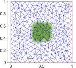
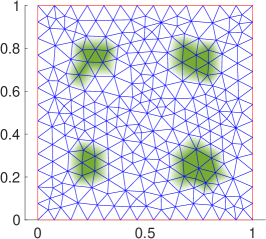
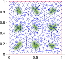
Figure 1. Initial spatial meshes ($\rho=0$) and supports $\omega_{i}$ of actuators $1_{\omega_{i}}$.

Since the mesh is unstructured and coarse the supports do not look like the rectangular supports we have the continuous level. We shall perform simulations is refinements of such mesh where the supports look more like those rectangular subdomains as we increase the number $\rho$ of refinements, as we can see in Fig. 2. The coarsest triangulation ${\mathcal{T}}^{0}$ corresponds to $\rho=0$, the refined triangulation ${\mathcal{T}}^{\rho}$ for $\rho\in\{1,2,3\}$ is obtained by dividing each triangle ${\mathcal{T}}^{\rho-1}_{k}$ of the triangulation ${\mathcal{T}}^{\rho-1}$ into $4$ congruent triangles by connecting the middle points of the edges of ${\mathcal{T}}^{\rho-1}_{k}$ (regular refinement).

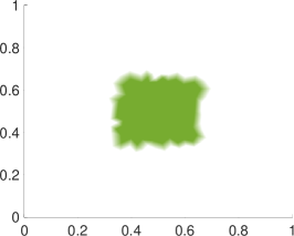
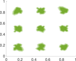
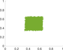
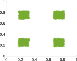
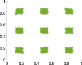
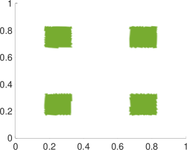
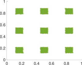
Figure 2. The $\rho$-th row shows the supports $\omega_{i}$ of actuators $1_{\omega_{i}}$ after $\rho$ regular refinement, $\rho\in\{1,2,3\}$.

We consider (3.1) under Neumann boundary conditions, and

$$\nu =0.1, \qquad a =-\tfrac{5}{2}+x_{1}-\left|\sin(6t+x_{1})\right|_{{\mathbb{R}}},$$ (4.1a)

$$y_{0} \coloneqq 1-2x_{1}x_{2}, \qquad b =\bigl{(}x_{1}+x_{2},\;\left|\cos(6t)x_{1}x_{2}\right|_{{\mathbb{R}}}\bigr{)}.$$ (4.1b)

The instability of the free dynamics is shown in Figure 3. Here, we used the coarsest spatial mesh with time step $k=0.01$ and the mesh obtained after $3$ regular refinements with time step $k=0.001$.

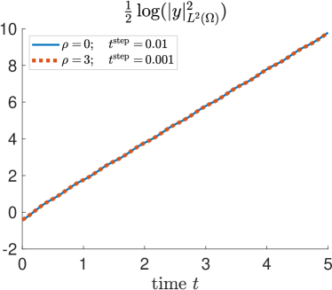
Figure 3. Free dynamics. Evolution of the norm of the solution.

We shall compare the time-truncated cost

$${\mathbf{J}}={\mathbf{J}}^{\rm feed}(y_{0},T)\coloneqq\tfrac{1}{2}\left|y^{\rm feed}\right|_{L^{2}((0,T),H)}^{2}+\beta\tfrac{1}{2}\left|u^{\rm feed}\right|_{L^{2}((0,T),{\mathbb{R}}^{M_{0}})}^{2},$$ (4.2)

associated to Riccati and oblique projection feedbacks, ${\rm feed}\in\{{\rm ricc},{\rm obli}\}$.

Note that $(a,b)$ in (4.1) is time-periodic with period $\tfrac{\pi}{6}$. We compute offline (prior to solve the parabolic equations), the input periodic Riccati feedback $\widehat{\mathbf{K}}={\mathbf{K}}$ as in (3.19), for corresponding actuators and coarse spatial mesh in Figure 1, for

$$t\in[\tau,\tau+\varpi],\quad\mbox{with}\quad\tau=0.1,\quad\varpi=\tfrac{\pi}{6},$$

(here, we could have chosen any $\tau\geq 0$) and with the parameters

$$\beta=1,\quad\overline{\mu}=\mu_{\rm ric}=1,\quad\mbox{and}\quad k_{\rm ric}=0.005.$$ (4.3)

Such feedback is then used as in (3.21) for refined meshes.

The explicit feedback (3.22) is computed online (while solving the equations), with the parameter

$$\lambda=1.$$

Since in the time interval $(0,+\infty)$, the cost (2.21c) is minimized by the Riccati feedback, we may expect to have that, for large $T$,

$${\mathbf{J}}^{\rm ricc}(y_{0},T)\leq{\mathbf{J}}^{\rm obli}(y_{0},T).$$ (4.4)

To construct the feedback in (3.22), as auxiliary eigenfunctions we have chosen the Cartesian products of the first $M_{0}^{\frac{1}{2}}$ one-dimensional (Neumann) eigenfunctions (as proposed in [38, sect. 4.8.1])

$${\mathcal{E}}_{M_{0}} =\mathop{\rm span}\nolimits\left\{e_{{\mathbf{j}}}\mid{\mathbf{j}}=({\mathbf{j}}_{1},{\mathbf{j}}_{2})\in\{1,2,\dots,M_{0}^{\frac{1}{2}}\}^{2}\right\},\qquad M_{0}\in\{1,4,9\},$$ (4.5a)

$$e_{{\mathbf{j}}} \coloneqq\cos\left(({\mathbf{j}}_{1}-1)\pi x_{1}\right)\cos\left(({\mathbf{j}}_{2}-1)\pi x_{2}\right).$$ (4.5b)

4.1. Using one actuator

In Figure 5 we see that the explicit oblique projection feedback (3.22) for the case of $1$ actuator is not able to stabilize the system, while in Figure 5 we see that the Riccati feedback (3.21) is (for the given initial state $y_{0}$). The later was computed for the coarsest mesh, and we can also see that it is still able to stabilize the system exponentially for refined meshes (again, for the given initial state). Note that we cannot conclude, from the present simulation result corresponding to a single initial condition, that the Riccati feedback will stabilize the solutions corresponding to an arbitrary initial state.

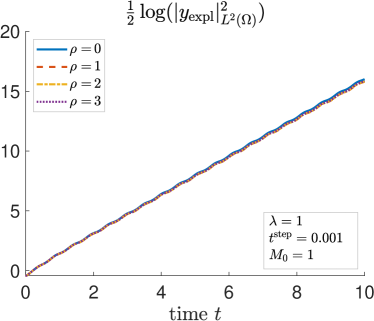
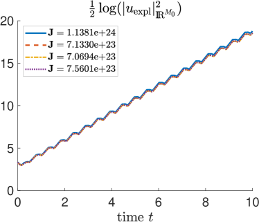
Figure 4. $M_{0}=1$. Oblique projection input feedback (3.22).

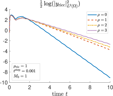
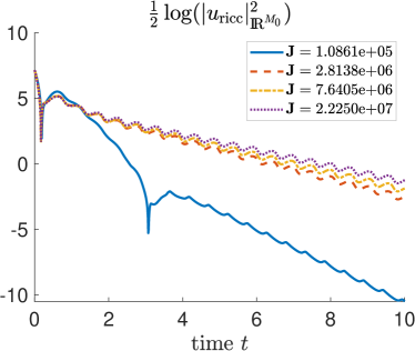
Figure 5. $M_{0}=1$. Riccati input feedback (3.21).

We also observe that the asked stability rate $\overline{\mu}=\mu_{\rm ric}=1$ is guaranteed for the coarsest mesh but not for the refined meshes. This shows that the Riccati feedback computed for the coarsest mesh does not lead to a good approximation of the Riccati operator solution and to the Riccati matrix solution for refined triangulations. This could also be a sign that one single actuator is not able to stabilize the system with exponential rate $\mu_{\rm ric}=1$ (for all initial states). Indeed for a rectangular with support $\omega=(\tfrac{1}{2}-r,\tfrac{1}{2}+r)$ centered at the center of our spatial square $\Omega$, this can be seen for the autonomous system corresponding to the reaction-convection pair $(a,b)=(c,(0,0))$ with small enough constant $c<0$, because for the solution of the system

$$\tfrac{\partial}{\partial t}z+(-\nu\Delta+{\mathbf{1}})z+cz=u1_{\omega},\qquad z(0)=z_{0}\coloneqq\cos(\pi x_{1})\cos(\pi x_{2}),$$

under Neumann boundary conditions, since $(z_{0},1_{\omega})_{L^{2}(\Omega)}=0$ and $z_{0}$ is an eigenfunction of $-\nu\Delta+{\mathbf{1}}+c{\mathbf{1}}$, we find that, for arbitrary control input $u\in L^{2}({\mathbb{R}}_{+},{\mathbb{R}})$ we will have

$$\tfrac{\partial}{\partial t}(P_{{\mathbb{R}}z_{0}}z)=(-2\pi^{2}\nu-1-c)P_{{\mathbb{R}}z_{0}}z,\quad P_{{\mathbb{R}}z_{0}}z(0)=z_{0},$$

where $P_{{\mathbb{R}}z_{0}}$ is the orthogonal projection onto the linear span ${{\mathbb{R}}z_{0}}$ of $\{z_{0}\}$. Hence,

$$P_{{\mathbb{R}}z_{0}}z(t)={\mathrm{e}}^{(-2\pi^{2}\nu-1-c)t}z_{0},$$

which diverges to $+\infty$ if $c<-2\pi^{2}\nu-1$.

4.2. Using four actuators

We increase the number of actuators (preserving the total volume covered by then). Figures 7 and 7 show that, with $4$ actuators, both oblique projection and Riccati based feedbacks are able to stabilize the system.

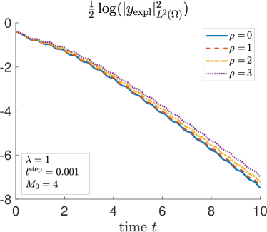
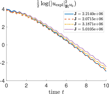
Figure 6. $M_{0}=4$. Oblique projection input feedback (3.22).

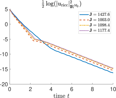
Figure 7. $M_{0}=4$. Riccati input feedback (3.21).

As expected, we also see that the quadratic cost functional (4.2) is smaller for Riccati.

Further, we see that an exponential stability rate $\mu\leq\lambda=1$ is provided by the oblique projection feedback and that an exponential stability rate $\mu>\mu_{\rm ric}=1$ is provided by the Riccati feedback. This confirms the theoretical results.

As we see in Fig. 1, we have a rough approximation of the $4$ actuators in the coarse mesh at least when compared with the approximation after $3$ refinements as in Fig 2. In spite of this fact, we still observe in Fig. 7 that the Riccati feedback computed for the coarsest mesh also provides a stability rate $\mu>\mu_{\rm ric}$ for the refined meshes. This is a first sign towards the validation the approach we propose of computing the Riccati input feedback operator in coarse meshes and using it in refined meshes.

4.3. Using nine actuators

To strengthen the validation of the proposed approach, we consider next the case of $9$ actuators, whose approximation in Fig. 1 is again rough when compared to the one obtained in the mesh after $3$ refinements shown in Fig 2. With $9$ actuators we see, in Figures 9 and 9, that both oblique projection and Riccati feedbacks are able to stabilize the system. Again we see that an exponential stability rate $\mu\leq\lambda=1$ is provided by the oblique projection feedback and that an exponential stability rate $\mu>\mu_{\rm ric}=1$ for both the coarsest and the refined meshes.

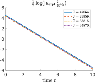
Figure 8. $M_{0}=9$. Oblique projection input feedback (3.22).

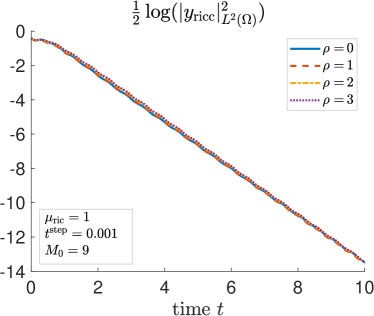
Figure 9. $M_{0}=9$. Riccati input feedback (3.21).

Furthermore, it is interesting to observe that, with the naked eye, we cannot see a difference on the behavior of the norm of the state in Figure 9. This shows that with the coarsest mesh we obtain already an accurate behavior of the controlled dynamics. This could be partially explained from the fact that the dynamics of the projection $z=P_{{\mathcal{E}}_{M_{0}}}y$ is explicitly imposed, $\dot{z}=-\lambda z$; see (2.5). Finally, we see that by taking a larger number $M_{0}$ of actuators the quadratic cost decreases for both feedbacks, note that this is a nontrivial observation because, in particular, by construction (following [38, sect. 4.8.1]), see Fig. 2, last row) the total volume (area) covered by the actuators is independent of the number of actuators. Our spatial domain is partitioned into $M_{0}$ rescaled copies of itself, and a rescaled actuator-subdomain is placed in each copy.

4.4. Performance of algorithm solving the periodic Riccati equation

In Fig. 10 we show the performance of iterative Algorithm 2, by showing the evolution of the error until it reaches a value smaller than ${\rm tol}=(N{\tt eps})^{\frac{1}{2}}\approx 2.4845\times 10^{-07}$. The error converges exponentially to zero, which confirms the result in Theorem 2.15. It is interesting to see that, after a suitable number $\underline{n}$ of iterations, the exponential rates for the cases $M_{0}\in\{1,4,9\}$ are close to each other, even likely the same with the naked eye as

$${\rm error}(n+1) \approx{\mathrm{e}}^{-0.4}{\rm error}(n)\approx{\mathrm{e}}^{-0.4(n+1-\underline{n})}{\rm error}(\underline{n}),\quad\mbox{for}\quad n\geq\underline{n},$$

where we have denoted

$${\rm error}(n) \coloneqq\left|\Pi^{n}(\tau)-\Pi^{n}(\tau+\varpi)\right|_{{\mathcal{L}}(L^{2}(\Omega)}.$$

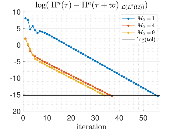
Figure 10. Error evolution for iterations of Algorithm 2.

We would like to report that, in the case of $4$ and $9$ actuators the Riccati time-step $k_{\rm ric}$ as in (4.3) turned out to be small enough so that step 11 in Algorithm 3 was never activated. Instead, in the case of $1$ actuators such step was often activated and more than once for some time instants $T$. That is, computing the optimal feedback for a single actuator took more time for each iteration of Algorithm 2. Roughly speaking this may suggest that stabilization with a single actuator is (at least; cf. section 4.1) more difficult (which somehow agrees with common sense).

5. Further remarks

We give additional details and comments on the followed procedure.

5.1. On the proposed strategy for solving the Riccati equations

For solving the algebraic Riccati equations within Algorithms 1 and 3, we have set the stopping criteria as $\frac{\left\|{\mathfrak{T}}_{({\mathbf{Y}},{\mathbf{B}},{\mathbf{C}})}(\mathbf{\Pi})\right\|}{\max\left\{1,\left\|\mathbf{\Pi}\right\|\right\}}<N^{\frac{1}{2}}{\tt eps}^{\frac{1}{2}}$, where ${\tt eps}\approx 10^{-16}$ is the Matlab epsilon/accuracy and $\left\|\raisebox{-1.07639pt}{\scalebox{1.25}{$\cdot$}}\right\|\coloneqq\left|\raisebox{-1.07639pt}{\scalebox{1.25}{$\cdot$}}\right|_{{\mathcal{L}}({\mathbb{R}}^{N})}$. This tolerance value is the minimal one used/proposed in the software [15], which we use hereafter.

Within Algorithm 2, for solving the periodic Riccati equation, we have set again the tolerance $\varepsilon=N^{\frac{1}{2}}{\tt eps}^{\frac{1}{2}}$ and replaced the norm in ${\mathcal{L}}(H)$ by the norm in ${\mathcal{L}}({\mathbb{R}}^{N})$ for the discretized equations.

Following Algorithm 3, we solve an algebraic Riccati equation at each time step. In order to speed the computations up, we could naturally think of taking a further linear approximation for the nonlinear unknown term in (3.18a), namely, we could take ${\mathbf{Z}}_{1}\coloneqq\frac{1}{2}(\mathbf{\Pi}^{r+1}{\mathbf{B}}{\mathbf{B}}^{\top}\mathbf{\Pi}^{r}+\mathbf{\Pi}^{r}{\mathbf{B}}{\mathbf{B}}^{\top}\mathbf{\Pi}^{r+1})$ instead of ${\mathbf{N}}\coloneqq\mathbf{\Pi}^{r}{\mathbf{B}}{\mathbf{B}}^{\top}\mathbf{\Pi}^{r}$. By taking such ${\mathbf{Z}}_{1}$ (linear on $\mathbf{\Pi}^{r}$) we would need to solve a single Lyapunov equation at each time step which would likely be cheaper/faster. An alternative could be to take an Adams–Bashforth linear extrapolation ${\mathbf{Z}}_{0}\coloneqq 2\mathbf{\Pi}^{r+1}{\mathbf{B}}{\mathbf{B}}^{\top}\mathbf{\Pi}^{r+1}-\mathbf{\Pi}^{r+2}{\mathbf{B}}{\mathbf{B}}^{\top}\mathbf{\Pi}^{r+2}$ (independent of $\mathbf{\Pi}^{r}$) instead of ${\mathbf{N}}$. However, by using an extra approximation for ${\mathbf{N}}$ we will induce an extra error which will back-propagate over the time interval $[\tau,\tau+\varpi]$, which we want to avoid (or minimize) when looking for the time $\varpi$-periodic solution of the time $\varpi$-periodic Riccati equation; see Algorithm 2.

5.2. On the Lyapunov equations

It is not our goal to discuss details on the numerical solution of the Lyapunov equation (3.8), but since it plays a crucial role in the solution of the algebraic Riccati equation, we refer the interested reader to the survey [20, sect. 5] where an ADI (alternating direction implicit) based iterative method is proposed for finding low-rank representations/approximations for the solution of Lyapunov matrix equations, and also to the related work [51] concerning Lyapunov operator equations in infinite-dimensional spaces and references therein. See also [42] for discussions on other methods. In this manuscript the Lyapunov equations were solved in factorized form with the matrix sign function [14, sect. IV].

5.3. On generalized Riccati equations

Note that in (3.14) we require the computation of the matrix ${\mathbf{X}}$ involving the inverse of the mass matrix, this is not a problem for the coarse discretizations we used to compute the solutions $\mathbf{\Pi}$ of the Riccati equations. In case we want or need to compute such solutions $\mathbf{\Pi}$ in fine discretizations, where we will have larger matrices, the inverse of the mass matrix can be an issue. In that case, an option to overcome this issue could be computing first the product $\mathbf{\Xi}={\mathbf{M}}^{-1}\mathbf{\Pi}{\mathbf{M}}^{-1}$, and then recover $\mathbf{\Pi}={\mathbf{M}}\mathbf{\Xi}{\mathbf{M}}$. Note that from (3.14) we find that $\mathbf{\Xi}$ solves a more general equation as follows

$${\mathbf{M}}\dot{\mathbf{\Xi}}{\mathbf{M}}+\widehat{\mathbf{X}}^{\top}\mathbf{\Xi}{\mathbf{M}}+{\mathbf{M}}\mathbf{\Xi}\widehat{\mathbf{X}}-{\mathbf{M}}\mathbf{\Xi}\widehat{\mathbf{B}}\widehat{\mathbf{B}}^{\top}\mathbf{\Xi}{\mathbf{M}}+{\mathbf{C}}^{\top}{\mathbf{C}}=0,$$

where $\widehat{\mathbf{X}}={\mathbf{M}}{\mathbf{X}}=-({\mathbf{S}}_{\nu}+{\mathbf{L}}^{0}+{\mathbf{L}}^{1}-\overline{\mu}{\mathbf{M}})$ and $\widehat{\mathbf{B}}={\mathbf{M}}{\mathbf{B}}$ (cf. [45, Equ. (15)], [21, below Equ. (8)], [32, Equ. (4.8)]). Thus, we can likely avoid the issues associated with the inverse of ${\mathbf{M}}$, with the expense of computing the solution of a more general equation. In any case, the solution of the Riccati equation $\mathbf{\Pi}$ is a full matrix at each instant of time time, for positive definite ${\mathbf{C}}^{\top}{\mathbf{C}}$, so we have anyway a constraint in the size of $\mathbf{\Pi}$. For the algebraic Riccati equation, in the case ${\mathbf{C}}$ has small rank (when compared to the size of ${\mathbf{M}}$) we can expect that $\mathbf{\Pi}$ is well approximated by products as $\mathbf{\Pi}_{\mathrm{f}}^{\top}\mathbf{\Pi}_{\mathrm{f}}$ where $\mathbf{\Pi}_{\mathrm{f}}$ has a small rank as well. For the solution of the differential Riccati equations this low-rank phenomenon is less clear. In any case, if $\mathbf{\Pi}$ is not necessarily positive definite, then we may need a different approach in Algorithm 3, where we have exploited the fact that $\mathbf{\Pi}$ is positive definite to guarantee the positive definiteness of ${\mathbf{Q}}$ for small time-step; see (3.18c).

6. Conclusions

At the theoretical level, we have shown that the explicit oblique projections based feedback operator introduced in [38] is able to stabilize parabolic equations with reaction-convection terms $A_{\rm rc}$ taking values in ${\mathcal{L}}(H,V^{\prime})+{\mathcal{L}}(V,H)$. We have also shown that the solution of the time-periodic Riccati equation can be found by an iterative process. At the numerical level, we have discussed general aspects from the finite-elements numerical implementation of stabilizing feedbacks, as the classical Riccati based feedbacks and oblique projections based feedbacks. The stabilizing performance of such feedbacks has been illustrated by results of simulations.

6.1. Oblique projections as an alternative to Riccati

Oblique projections feedbacks are an interesting alternative to the Riccati feedbacks, since they are easier to compute and implement numerically, and because we do not need to save the solution of the differential Riccati equation, prior to simulations. In particular, the oblique projections feedback input can be computed online in real time. Another disadvantage of Riccati based feedbacks is that its computation is unfeasible for general nonautonomous systems in the entire unbounded time interval. Thus we have restricted the numerical computations to the case of a time-periodic reaction-convection terms, where we can reduce the computations to a finite time interval with length equal to the time-period.

6.2. Oblique projections as a nonalternative to Riccati

An advantage of the Riccati based feedbacks is that it is less sensitive with respect to the number and location of the actuators, and it further minimizes the total spent energy (classical quadratic cost). So, if the minimization of the spent energy is important/asked in a given application and/or if we do not have an enough number of actuators at our disposal, then the oblique projections based feedbacks may be not an alternative to the Riccati based ones. In such case, we have to face the fact that for fine discretizations it is difficult, and maybe unfeasible, to compute and save the entire array with the solution of the input Riccati operator for each discrete instant of time, in the fixed (large) bounded time interval (e.g., for a large time-period). To circumvent this issue, we propose to compute the Riccati feedback for a coarse mesh, and use it to construct an “extended” feedback allowing us to perform simulations in appropriately refined meshes, in both spatial and temporal domains. We presented simulations showing that such strategy provides us with a stabilizing feedback.

6.3. Open questions. Possible future works

Concerning Riccati feedbacks, it is clear that the coarsest spatial and temporal meshes must be “fine enough”. It would be interesting to investigate this point in order to quantify “how fine” such meshes must be taken. This is expected to depend on the given system (free) dynamics. We have used Algorithm 2 to compute the solution of the time-periodic operator differential Riccati equation. This approach will be expensive (time consuming) if the time-period $\varpi$ is large. Though we expect the error in Algorithm 2 to convergence exponentially to zero (cf. Thm. 2.15 and Fig. 10), the exponential rate can be relatively small and we will need a large number of iterations. Thus it would be interesting to know more about such rate. In [29] the authors are able to compute the solution for large time-periods in a relatively short time. Unfortunately, from the results reported in [29, sect. 5] the methods evaluated/compared in the same reference are likely not appropriate for computing the periodic matrix Riccati solution for matrices as large as those coming from finite-element discretizations of partial differential equations; the sizes of the matrices considered [29, sect. 5.1.1, Table 2, and sect. 5.1.2] are far from the number of nodes of the mesh in Fig. 1.

Acknowledgments. The author acknowledges partial support from the Upper Austria Government and the Austrian Science Fund (FWF): P 33432-NBL.

References

• [1] U.M. Ascher, S.J. Ruuth, and B.T.R. Wetton. Implicit-explicit methods for time-dependent partial differential equations. SIAM J. Numer. Anal., 32(3):797–823, 1995. URL: http://www.jstor.org/stable/2158449.
• [2] B. Azmi and S. S. Rodrigues. Oblique projection local feedback stabilization of nonautonomous semilinear damped wave-like equations. J. Differential Equations, 269(7):6163–9192, 2020. doi:10.1016/j.jde.2020.04.033.
• [3] A. Azouani and E. S. Titi. Feedback control of nonlinear dissipative systems by finite determining parameters – a reaction-diffusion paradigm. Evol. Equ. Control Theory, 3(4):579–594, 2014. doi:10.3934/eect.2014.3.579.
• [4] M. Badra, D. Mitra, M. Ramaswamy, and J.-P. Raymond. Stabilizability of time-periodic evolution equations by finite dimensional controls. SIAM J. Control Optim., 58(3):1735–1768, 2020. doi:10.1137/19M1273451.
• [5] M. Badra and T. Takahashi. Stabilization of parabolic nonlinear systems with finite dimensional feedback or dynamical controllers: Application to the Navier–Stokes system. SIAM J. Control Optim., 49(2):420–463, 2011. doi:10.1137/090778146.
• [6] H. T. Banks and K. Ito. A numerical algorithm for optimal feedback gains in high dimensional linear quadratic regulator problems. SIAM J. Control Optim., 29(3):499–515, 1991. doi:10.1137/0329029.
• [7] H. T. Banks and K. Kunisch. The linear regulator problem for parabolic systems. SIAM J. Control Optim., 22(5):684–698, 1984. doi:10.1155/S1024123X00001320.
• [8] E. Bänsch, P. Benner, J. Saak, and H. K. Weichelt. Riccati-based boundary feedback stabilization of incompressible Navier–Stokes flows. SIAM J. Sci. Comput., 37(2):A832–A858, 2015. doi:10.1137/140980016.
• [9] V. Barbu. Stabilization of Navier–Stokes Flows. Comm. Control Engrg. Ser. Springer-Verlag London, 2011. doi:10.1007/978-0-85729-043-4.
• [10] V. Barbu. Boundary stabilization of equilibrium solutions to parabolic equations. IEEE Trans. Automat. Control, 58(9):2416–2420, 2013. doi:10.1109/TAC.2013.2254013.
• [11] V. Barbu, I. Lasiecka, and R. Triggiani. Abstract settings for tangential boundary stabilization of Navier–Stokes equations by high- and low-gain feedback controllers. Nonlinear Anal., 64(12):2704–2746, 2006. doi:10.1016/j.na.2005.09.012.
• [12] V. Barbu, S. S. Rodrigues, and A. Shirikyan. Internal exponential stabilization to a nonstationary solution for 3D Navier–Stokes equations. SIAM J. Control Optim., 49(4):1454–1478, 2011. doi:10.1137/100785739.
• [13] V. Barbu and R. Triggiani. Internal stabilization of Navier–Stokes equations with finite-dimensional controllers. Indiana Univ. Math. J., 53(5):1443–1494, 2004. doi:10.1512/iumj.2004.53.2445.
• [14] P. Benner. A matlab repository for model reduction based on spectral projection. In Proceedings of the 2006 IEEE Conference on Computer Aided Control Systems Design, pages 19–24, October 4-6 2006. doi:10.1109/CACSD-CCA-ISIC.2006.4776618.
• [15] P. Benner. MORLAB - Model Order Reduction LABoratory (version 1.0), package software, 2006. URL: http://www.mpi-magdeburg.mpg.de/projects/morlab.
• [16] P. Benner. Partial stabilization of descriptor systems using spectral projectors. In Numerical Linear Algebra in Signals, Systems and Control, chapter 3, pages 55–76. Springer, Dordrecht, 2011. doi:10.1007/978-94-007-0602-6_3.
• [17] P. Benner, Z. Bujanović, P. Kürschner, and J. Saak. A numerical comparison of different solvers for large-scale, continuous-time algebraic Riccati equations and LQR problems. SIAM J. Sci. Comput., 42(2):A957–A996, 2020. doi:10.1137/18M1220960.
• [18] P. Benner, A.J. Laub, and V. Mehrmann. Benchmarks for the numerical solution of algebraic Riccati equations. IEEE Control Systems Magazine, 17(5):18–28, 1997. doi:10.1109/37.621466.
• [19] P. Benner, J.-R. Li, and Th. Penzl. Numerical solution of large-scale Lyapunov equations, Riccati equations, and linear-quadratic optimal control problems. Numer. Linear Algebra Appl., 15(9):755–777, 2008. doi:10.1002/nla.622.
• [20] P. Benner and J. Saak. Numerical solution of large and sparse continuous time algebraic matrix Riccati and Lyapunov equations: a state of the art survey. GAMM-Mitt., 36(1):32–52, 2013. doi:10.1002/gamm.201310003.
• [21] T. Breiten, S. Dolgov, and M. Stoll. Solving differential Riccati equations: a nonlinear space-time method using tensor trains. Numer. Algebra Control Optim., 2020. doi:doi:10.3934/naco.2020034.
• [22] T. Breiten and K. Kunisch. Riccati-based feedback control of the monodomain equations with the FitzHugh–Nagumo model. SIAM J. Control Optim., 52(6):4057–4081, 2014. doi:10.1137/140964552.
• [23] T. Breiten, K. Kunisch, and S. S. Rodrigues. Feedback stabilization to nonstationary solutions of a class of reaction diffusion equations of FitzHugh–Nagumo type. SIAM J. Control Optim., 55(4):2684–2713, 2017. doi:10.1137/15M1038165.
• [24] B. Cockburn, D. A. Jones, and E. S. Titi. Estimating the number of asymptotic degrees of freedom for nonlinear dissipative systems. Math. Comp., 66(219):1073–1087, 1997. doi:10.1090/S0025-5718-97-00850-8.
• [25] R. Curtain and A. J. Pritchard. The infinite-dimensional Riccati equation for systems defined by evolution operators. SIAM J. Control Optim., 14(5):951–983, 1976. doi:10.1137/0314061.
• [26] R. Datko. Uniform asymptotic stability of evolutionary processes in a Banach space. SIAM J. Math. Anal., 3(3):428–445, 1972. doi:10.1137/0503042.
• [27] M. Ethier and Y. Bourgault. Semi-implicit time-discretization schemes for the bidomain model. SIAM J. Numer. Anal., 46(5):2443–2468, 2008. doi:10.1137/070680503.
• [28] J. S. Gibson. The Riccati integral equations for optimal control problems on Hilbert spaces. SIAM J. Control Optim., 17(4):537–565, 1979. doi:10.1137/0317039.
• [29] S. Gusev, S. Johansson, B. Kågström, A. Shiriaev, and A. Varga. A numerical evaluation of solvers for the periodic Riccati differential equation. BIT Numer. Math., 50(2):301–329, 2010. doi:10.1007/s10543-010-0257-5.
• [30] A. Halanay, C. M. Murea, and C. A. Safta. Numerical experiment for stabilization of the heat equation by Dirichlet boundary control. Numer. Funct. Anal. Optim., 34(12):1317–1327, 2013. doi:10.1080/01630563.2013.808210.
• [31] Y. He and W. Sun. Stability and convergence of the Crank–Nicolson/Adams–Bashforth scheme for the time-dependent Navier–Stokes equations. SIAM J. Numer. Anal., 45(2):837–869, 2007. doi:10.1137/050639910.
• [32] J. Heiland. A differential-algebraic Riccati equation for applications in flow control. SIAM J. Control Optim., 54(2):718–739, 2016. doi:10.1137/151004963.
• [33] S. Kesavan and J.-P. Raymond. On a degenerate Riccati equation. Control Cybernet., 38(4B):1393–1410, 2009. URL: http://control.ibspan.waw.pl:3000/mainpage/index.
• [34] A. A. Kornev. The method of asymptotic stabilization to a given trajectory based on a correction of the initial data. Comput. Math. Math. Phys., 46(1):34–48, 2006. doi:10.1134/S0965542506010064.
• [35] A. Kröner and S. S. Rodrigues. Remarks on the internal exponential stabilization to a nonstationary solution for 1D Burgers equations. SIAM J. Control Optim., 53(2):1020–1055, 2015. doi:10.1137/140958979.
• [36] M. Krstic, L. Magnis, and R. Vazquez. Nonlinear stabilization of shock-like unstable equilibria in the viscous Burgers PDE. IEEE Trans. Automat. Control, 53(7):1678–1683, 2008. doi:10.1109/TAC.2008.928121.
• [37] M. Krstic, L. Magnis, and R. Vazquez. Nonlinear control of the viscous Burgers equation: Trajectory generation, tracking, and observer design. J. Dyn. Syst. Meas. Control, 131(2):021012(1–8), 2009. doi:10.1115/1.3023128.
• [38] K. Kunisch and S. S. Rodrigues. Explicit exponential stabilization of nonautonomous linear parabolic-like systems by a finite number of internal actuators. ESAIM Control Optim. Calc. Var., 25, 2019. Art 67. doi:10.1051/cocv/2018054.
• [39] P. Kunkel and V. Mehrmann. Numerical solution of differential algebraic Riccati equations. Linear Algebra Appl., 137/138:39–66, 1990. doi:10.1016/0024-3795(90)90126-W.
• [40] P. Lancaster and M. Tismenetsky. The Theory of Matrices. Academic Press, 2nd edition, 1985. URL: https://www.elsevier.com/books/the-theory-of-matrices/lancaster/978-0-08-051908-1.
• [41] C. Lefter. Feedback stabilization of 2D Navier–Stokes equations with Navier slip boundary conditions. Nonlinear Anal., 70(1):553–562, 2009. doi:10.1016/j.na.2007.12.026.
• [42] A. Lu and E. L. Wachspress. Solution of Lyapunov equations by alternating direction implicit iteration. Computers Math. Applic., 21(9):43–58, 1991. doi:10.1016/0898-1221(91)90124-M.
• [43] A. Lunardi. Stabilizability of time-periodic parabolic equations. SIAM J. Control Optim., 29(4):810–828, 1991. doi:10.1137/0329044.
• [44] E. Lunasin and E. S. Titi. Finite determining parameters feedback control for distributed nonlinear dissipative systems – a computational study. Evol. Equ. Control Theory, 6(4):535–557, 2017. doi:10.3934/eect.2017027.
• [45] A. Malqvist, A. Persson, and T. Stillfjord. Multiscale differential Riccati equarions for linear quadratic regulator problems. SIAM J. Sci. Comput., 40(4):A2406–A2426, 2018. doi:10.1137/17M1134500.
• [46] M. Marion and R. Temam. Navier–Stokes equations: Theory and approximation. In Handbook of Numerical Analysis, volume VI, pages 503–689. Elsevier Science, 1998. doi:10.1016/S1570-8659(98)80010-0.
• [47] K. Morris. Linear-quadratic optimal actuator location. IEEE Trans. Automat. Control, 56(1):113–124, 2011. doi:10.1109/TAC.2010.2052151.
• [48] I. Munteanu. Normal feedback stabilization of periodic flows in a three-dimensional channel. Numer. Funct. Anal. Optim., 33(6):611–637, 2012. doi:10.1080/01630563.2012.662198.
• [49] I. Munteanu. Normal feedback stabilization of periodic flows in a two-dimensional channel. J. Optim. Theory Appl., 152(2):413–438, 2012. doi:10.1007/s10957-011-9910-7.
• [50] E. M. D. Ngom, A. Sène, and D. Y. Le Roux. Global stabilization of the Navier–Stokes equations around an unstable equilibrium state with a boundary feedback controller. Evol. Equ. Control Theory, 4(1):89–106, 2015. doi:10.3934/eect.2015.4.89.
• [51] M.R. Opmeer, T. Reis, and W. Wollner. Finite-rank ADI iteration for operator Lyapunov equations. SIAM J. Control Optim., 51(5):4084–4117, 2013. doi:10.1137/120885310.
• [52] D. Phan and S. S. Rodrigues. Stabilization to trajectories for parabolic equations. Math. Control Signals Syst., 30(2):(Art. 11), 2018. doi:10.1007/s00498-018-0218-0.
• [53] J.-P. Raymond. Stabilizability of infinite-dimensional systems by finite-dimensional controls. Comput. Methods Appl. Math., 19(4):797–811, 2019. doi:10.1515/cmam-2018-0031.
• [54] J.-P. Raymond and L. Thevenet. Boundary feedback stabilization of the two-dimensional Navier–Stokes equations with finite-dimensional controllers. Discrete Contin. Dyn. Syst., 27(3):1159–1187, 2010. doi:10.3934/dcds.2010.27.1159.
• [55] S. S. Rodrigues. Semiglobal exponential stabilization of nonautonomous semilinear parabolic-like systems. Evol. Equ. Control Theory, 9(3):635–672, 2020. doi:10.3934/eect.2020027.
• [56] S. S. Rodrigues. Oblique projection exponential dynamical observer for nonautonomous linear parabolic-like equations. SIAM J. Control Optim., 59(1):464–488, 2021. doi:10.1137/19M1278934.
• [57] S. S. Rodrigues and K. Sturm. On the explicit feedback stabilization of one-dimensional linear nonautonomous parabolic equations via oblique projections. IMA J. Math. Control Inform., 37(1):175–207, 2020. doi:10.1093/imamci/dny045.
• [58] D. Tsubakino, M. Krstic, and Sh. Hara. Backstepping control for parabolic PDEs with in-domain actuation. In Proceedings of the American Control Conference (ACC), Montréal, Canada, pages 2226–2231, 2012. doi:10.1109/ACC.2012.6315358.
• [59] V. M. Ungureanu and V. Dragan. Nonlinear differential equations of Riccati type on ordered Banach spaces. In Electron. J. Qual. Theory Differ. Equ., Proc. 9’th Coll. QTDE, number 17, pages 1–22, 2012. doi:10.14232/ejqtde.2012.3.17.
• [60] A. Varga. On solving periodic Riccati equations. Numer. Linear Algebra Appl., 15(9):809–835, 2008. doi:10.1002/nla.604.
• [61] S. Wang and F. Woittennek. Backstepping-method for parabolic systems with in-domain actuation. IFAC Proceedings Volumes, 46(26):43–48, 2013. doi:10.3182/20130925-3-FR-4043.00049.
• [62] F. Woittennek, S. Wang, and T. Knüeppel. Backstepping design for parabolic systems with in-domain actuation and Robin boundary conditions. IIFAC Proceedings Volumes, 47(3):5175–5180, 2014. doi:10.3182/20140824-6-ZA-1003.02285.
• [63] M.Y. Wu. A note on stability of linear time-varying systems. IEEE Trans. Automat. Control, 19(2):162, 1974. doi:10.1109/TAC.1974.1100529.
• [64] J. Zabczyk. Remarks on the algebraic Riccati equation in Hilbert space. Appl. Math. Optim., 2(3):251–258, 1975. doi:10.1007/BF01464270.
• [65] T. Zhang, J. Jin, and Y. HuangFu. The Crank–Nicolson/Adams–Bashforth scheme for the Burgers equation with $H^{1}$ and $H^{2}$ initial data. Appl. Num. Math., 125:103–142, 2018. doi:10.1016/j.apnum.2017.10.009.