Semileptonic $B_{s}\to K_{0}^{*}(1430)$ transitions with the light-cone sum rules

Abstract

In the $\rm SU(3)_{F}$ symmetry limit, using two- and three-particle distribution amplitudes of $B^{\pm}$-meson for $B_{s}$, the transition form factors of semileptonic $B_{s}\to K_{0}^{*}(1430)$ decays are calculated in the framework of the light-cone sum rules. The two-particle distribution amplitudes, $\varphi_{{}_{+}}(\omega)$ and $\varphi_{{}_{-}}(\omega)$ have the most important contribution in estimation of the form factors $f_{+}(q^{2})$, $f_{-}(q^{2})$ and $f_{T}(q^{2})$. The knowledge of the behavior of $\varphi_{{}_{+}}(\omega)$ is still rather limited. Therefore, we consider three different parametrizations for the shapes of $\varphi_{{}_{+}}(\omega)$ that are derived from the phenomenological models. Using the form factors $f_{+}$, $f_{-}$ and $f_{T}$, the semileptonic $B_{s}\to K_{0}^{*}(1430)l\bar{\nu_{l}}$ and $B_{s}\to K_{0}^{*}(1430)l\bar{l}/\nu\bar{\nu}$, $l=e,\mu,\tau$ decays are analyzed. The branching fractions for the aforementioned decays, in addition the longitudinal lepton polarization asymmetries are calculated. A comparison between our results with predictions of other approaches is provided.

I Introduction

The scalar meson is a meson with total spin $0$ and even parity. They are often produced in proton-antiproton annihilation, decays of heavy flavor mesons, meson-meson scattering, and radiative decays of vector mesons. Among the scalar mesons, study of the light scalar mesons up to $1.5\,\mbox{GeV}$ is important because their quark content is still a common problem for high energy physics and may be explained in a number of different ways, for example, considering as a meson-meson molecules state molecules or as a tetraquark multiplet tetraquark .

According to the quark model, the scalar mesons about $1\,\mbox{GeV}$ are arranged into two $SU(3)$ nonets, in two scenarios:

Scenario 1 (S1): the light scalar mesons are assumed to compose from two quarks. The nonet mesons below $1\,\mbox{GeV}$ are treated as the lowest lying states, and the nonet mesons near $1.5\,\mbox{GeV}$ are the excited states corresponding to the lowest lying states.

Scenario 2 (S2): the nonet mesons below $1\,\mbox{GeV}$ may be considered as four-quark bound states, and the other nonet mesons are composed from two quarks and viewed as the lowest lying states.

Both scenarios in quark model agree that $K^{*}_{0}(1430)$ with the mass of greater than $1\,\mbox{GeV}$ is a scalar meson with two quarks dominated by the $s\bar{u}$ or $s\bar{d}$ state. However in S1, it is regarded as an excited state, and in S2, it is seen as a ground state. In the framework of the light-cone sum rules (LCSR), differences between $K^{*}_{0}(1430)$ states in the two scenarios are applied through different distribution amplitudes (DA’s) and decay constants CheChuYan .

In this paper, our aim is to consider the semileptonic transitions of $B_{s}$ to $K_{0}^{*}(1430)$ in the LCSR using the $B_{s}$-meson DA’s. In usual, the LCSR method is applied to calculate the form factors of the heavy-to-light decays by utilizing the light meson DA’s. For this purpose, two-point correlation function is written based on the light meson. Therefore, light-cone distribution amplitudes (LCDA’s) of the light meson appear in theoretical calculations of the correlation function Ruckl ; Simma ; Belyaev ; Weinzierl ; BBraun ; Bagan ; Ball ; Zwicky ; BZwicky . The LCDA’s of the light mesons are related to the dynamics of partons in long distance. Still, there is very limited knowledge of the nonperturbative parameters determining these LCDA’s. In the case of the light scalar mesons, including $K_{0}^{*}(1430)$, this problem is twofold because their internal structures are basically unknown. For this reason, it is necessary to use a method of calculation that is independent of the DA’s of the scalar mesons.

In a new approach to the LCSR method related to the semileptonic $B$ decays, it was proposed to insert the correlation function between vacuum and $B$-meson Offen . In this technique the so-called soft or endpoint, the correlation function is expanded in terms of the DA’s of $B$-meson, near the light-cone region KMO ; BrKhod . Therefore, the transition form factors for exclusive decays of $B$ to light mesons are connected to the DA’s that depend on the dynamical information of $B$-meson. Two-particle DA of $B$-meson, $\varphi_{{}_{+}}(\omega)$ plays a particularly prominent role in this new approach to exclusive semileptonic decays. The knowledge of the behavior of $\varphi_{{}_{+}}(\omega)$ is still rather limited due to the poor understanding of nonperturbative QCD dynamics (for instance, see Refs. BraManash ; GalNeu ; XuZhao ; ZhaRad ). So far, several models for the shape of $\varphi_{{}_{+}}(\omega)$ have been proposed based on the QCD sum rules (QCDSR) Grozin ; Braun , the LCSR GenonSachrajda ; Kou ; LeeNeubert ; BellFeldmann ; FeldLange ; WangShen ; BeneBraun , and the QCD factorization JiMan . Also, the functional form of the three-particle $B$-meson DA’s have been estimated in several models KMO ; JiMan ; ShenWangWei .

In this work, the form factors of the semileptonic $B_{s}\to K_{0}^{*}(1430)$ transitions are investigated in the new approach of the LCSR with the two- and three-particle DA’s of $B_{s}$-meson in the $\rm SU(3)_{F}$ symmetry limit. Utilizing these form factors, the semileptonic $B_{s}\to K_{0}^{*}(1430)l\bar{\nu_{l}}$ and $B_{s}\to K_{0}^{*}(1430)l\bar{l}/\nu\bar{\nu}$, $l=e,\mu,\tau$ decays are analyzed. In the standard model (SM), the rare semileptonic $B_{s}\to K_{0}^{*}(1430)l\bar{l}$ decays occur at loop level instead of tree level, by electroweak penguin and weak box diagrams via the flavor changing neutral current (FCNC) transitions of $b\to dl^{+}l^{-}$ at quark level. In particle physics, reliable considering of the FCNC decays of $B$-meson is very important since they are sensitive to new physics (NP) contributions to penguin operators. So, to test the SM and look for NP, we need to determine the SM predictions for FCNC decays and compare these results to the corresponding experimental values.

This work is organized as follows: In Sec II, according to the effective weak Hamiltonian of the FCNC transition $b\to d~{}l^{+}l^{-}$, the form factors of the semileptonic $B_{s}\to K_{0}^{*}$ decays are calculated with the LCSR model using the $B_{s}$-meson DA’s. These form factors are basic parameters in studying the forward-backward asymmetry, longitudinal lepton polarization asymmetry and branching fraction of semileptonic decays. Our numerical and analytical results and their comparison with the predictions of other approaches are presented in Sec III. The last section is dedicated to conclusion. Future experimental measurement can give valuable information about these aforesaid decays and the nature of the scalar meson $K_{0}^{*}(1430)$.

II $B_{s}\to K_{0}^{*}\,l^{+}l^{-}$ Form Factors with the LCSR

According to the effective weak Hamiltonian of the $b\to d~{}l^{+}l^{-}$ transition presented in Appendix, the matrix element for the FCNC decay $b\to d$ can be written as:

$${\cal M}=\frac{G_{F}\alpha}{2\sqrt{2}\pi}V_{tb}V_{td}^{*}\Bigg{[}C_{9}^{\rm eff}\,\,\bar{d}\gamma_{\mu}(1-\gamma_{5})b~{}\overline{l}\gamma_{\mu}l+C_{10}\,\,\bar{d}\gamma_{\mu}(1-\gamma_{5})b~{}\overline{l}\gamma_{\mu}\gamma_{5}\l-2\,C_{7}^{\rm eff}\,\,\frac{m_{b}}{q^{2}}\,\bar{d}~{}i\sigma_{\mu\nu}q^{\nu}(1+\gamma_{5})b~{}\overline{l}\gamma_{\mu}l\Bigg{]},$$ (1)

where $G_{F}$ is the Fermi constant, $\alpha$ is the fine structure constant at $Z$ mass scale, and $V_{ij}$ are elements of the Cabbibo- Kobayashi-Maskawa (CKM) matrix. $\bar{d}\gamma_{\mu}(1-\gamma_{5})b$ and $\bar{d}\sigma_{\mu\nu}q^{\nu}(1+\gamma_{5})b$ are the transition currents denoted with $J^{V-A}_{\mu}$ and $J^{T}_{\mu}$, respectively. This decay amplitude also contains two effective Wilson coefficients $C_{7}^{\rm eff}$ and $C_{9}^{\rm eff}$, where $C_{7}^{\rm eff}=C_{7}-C_{5}/3-C_{6}$ and $C_{9}^{\rm eff}$ is explained in Appendix.

To investigate the form factors of $B_{s}\to K_{0}^{*}l^{+}l^{-}$ decays via the LCSR, the two-point correlation functions are constructed from the transition currents $J_{\mu}^{V-A(T)}$, and interpolating current $J^{K_{0}^{*}}$ of the scalar meson $K_{0}^{*}$, inserted between vacuum and $B_{s}$-meson as follows:

$$\Pi_{\mu}^{V-A(T)}(p^{\prime},q)=i\int{d^{4}x}~{}e^{ip^{\prime}.x}\langle 0|T\left\{J^{K_{0}^{*}}(x)J_{\mu}^{V-A(T)}(0)\right\}|B_{s}(p)\rangle,$$ (2)

where $T$ is the time ordering operator, $J^{K_{0}^{*}}=\bar{s}(x)d(x)$ and $q=p-p^{\prime}$. The external momenta $p^{\prime}$ and $q$ are related to the interpolating and transition currents, $J^{K_{0}^{*}}$ and $J_{\mu}^{V-A(T)}$ respectively, so that $p^{2}=(p^{\prime}+q)^{2}=m^{2}_{B}$. The leading-order diagram for $B_{s}\rightarrow K_{0}^{*}l^{+}l^{-}$ decays is depicted in Fig. 1.

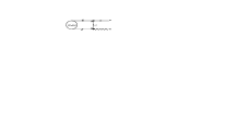
Figure 1: leading-order diagram for $B_{s}\rightarrow K_{0}^{*}l^{+}l^{-}$ decays.

The correlation functions in Eq. (2) are complex quantities and have two aspects: phenomenological and theoretical. Hadronic parameters like form factors appear in the phenomenological or physical representation of the correlation functions. The theoretical or QCD side of the correlation functions is obtained in terms of the DA’s of $B_{s}$-meson. Equating coefficients of the corresponding lorentz structures from both representations through the dispersion relation,

$$\Pi_{\mu}(p^{\prime},q)=\frac{1}{\pi}\int_{0}^{\infty}ds\frac{\mbox{Im}\,\Pi_{\mu}(s)}{s-p^{\prime 2}}\,,$$ (3)

and applying Borel transformation to suppress the contributions of the higher states and continuum, the form factors are calculated from the LCSR.

Inserting a complete set of intermediate states with the same quantum number as the interpolating current $J^{K_{0}^{*}}$, in Eq. (2), and isolating the pole term of the lowest scalar meson $K_{0}^{*}$, and then applying Fourier transformation, the phenomenological representations of the correlation functions are obtained, as follows:

$$\Pi_{\mu}^{V-A(T)}(p^{\prime},q) = \frac{1}{m_{K_{0}^{*}}^{2}-p^{\prime 2}}\langle 0|J^{K_{0}^{*}}(p^{\prime})|K_{0}^{*}(p^{\prime})\rangle\langle K_{0}^{*}(p^{\prime})|J^{V-A(T)}_{\mu}|B_{s}(p)\rangle$$ (4)

$$+ \sum_{h}\,\frac{1}{m_{h}^{2}-p^{\prime 2}}\langle 0|J^{K_{0}^{*}}(p^{\prime})|h(p^{\prime})\rangle\langle h(p^{\prime})|J^{V-A(T)}_{\mu}|B_{s}(p)\rangle\,.$$

To continue, we define the spectral density functions of higher resonances and the continuum of states as

$$\rho^{h,V-A(T)}_{\mu}(s)\equiv\pi\,\sum_{h}\,\langle 0|J^{K_{0}^{*}}(p^{\prime})|h(p^{\prime})\rangle\langle h(p^{\prime})|J^{V-A(T)}_{\mu}|B_{s}(p)\rangle\,\delta(s-m^{2}_{h}).$$ (5)

Inserting the spectral density functions in Eq. (4), the correlation functions are obtained as

$$\Pi^{V-A(T)}_{\mu}(p^{\prime},q) = \frac{1}{m_{K_{0}^{*}}^{2}-p^{\prime 2}}\langle 0|J^{K_{0}^{*}}(p^{\prime})|K_{0}^{*}(p^{\prime})\rangle\langle K_{0}^{*}(p^{\prime})|J^{V-A(T)}_{\mu}|B_{s}(p)\rangle+\frac{1}{\pi}\int_{s_{0}}^{\infty}ds\frac{\rho_{\mu}^{h,{V-A(T)}}(s)}{s-p^{\prime 2}},$$ (6)

where $s_{0}$ is the continuum threshold of $K_{0}^{*}$ meson. The matrix element, $\langle 0|J^{K_{0}^{*}}|K_{0}^{*}\rangle=f_{K_{0}^{*}}m_{K_{0}^{*}}$, where $f_{K_{0}^{*}}$ is the leptonic decay constant of the scalar meson $K_{0}^{*}$. Considering parity and using Lorentz invariance, the transition matrix elements, $\langle K_{0}^{*}(p^{\prime})|J^{V-A(T)}_{\mu}|B_{s}(p)\rangle$, can be parametrized as:

$$\langle K_{0}^{*}(p^{\prime})|J^{V-A}_{\mu}|B_{s}(p)\rangle = i\left[P_{\mu}f_{+}(q^{2})\,+\,q_{\mu}f_{-}(q^{2})\right],$$

$$\langle K_{0}^{*}(p^{\prime})|J^{T}_{\mu}|B_{s}(p)\rangle = -\frac{1}{m_{B_{s}}+m_{K_{0}^{*}}}\left[P_{\mu}q^{2}-q_{\mu}(m_{B_{s}}^{2}-m_{K_{0}^{*}}^{2})\right]f_{T}(q^{2}),$$ (7)

where $f_{+}(q^{2})$, $f_{-}(q^{2})$ and $f_{T}(q^{2})$  are the transition form factors, which only depend on the momentum transfer squared $q^{2}$, $P_{\mu}=(p^{\prime}+p)_{\mu}$, and $q_{\mu}=(p-p^{\prime})_{\mu}$. Substituting Eq. (II) in Eq. (6), we obtain

$$\Pi^{V-A}_{\mu}(p^{\prime},q) = if_{K_{0}^{*}}m_{K_{0}^{*}}\left[\frac{P_{\mu}f_{+}(q^{2})\,+\,q_{\mu}f_{-}(q^{2})}{m_{K_{0}^{*}}^{2}-p^{\prime 2}}\right]+\frac{1}{\pi}\int_{s_{0}}^{\infty}ds\frac{\rho_{\mu}^{h,{V-A}}(s)}{s-p^{\prime 2}}\,,$$

$$\Pi^{T}_{\mu}(p^{\prime},q) = -\frac{f_{K_{0}^{*}}m_{K_{0}^{*}}}{m_{B_{s}}+m_{K_{0}^{*}}}\left[\frac{P_{\mu}q^{2}-q_{\mu}(m_{B_{s}}^{2}-m_{K_{0}^{*}}^{2})}{m_{K_{0}^{*}}^{2}-p^{\prime 2}}\right]f_{T}(q^{2})+\frac{1}{\pi}\int_{s_{0}}^{\infty}ds\frac{\rho_{\mu}^{h,{T}}(s)}{s-p^{\prime 2}}\,.$$ (8)

To extract the theoretical or QCD side, the correlation functions in Eq. (2) are expanded in the limit of large $m_{b}$ in heavy quark effective theory (HQET). In the HQET, the relation between the momentum and four-velocity of $B_{s}$-meson is as: $p=m_{b}v+k$, where $k$ is the residual momentum. Using the relation $p=q+p^{\prime}$ and $p=m_{b}v+k$, the four-momentum transfer $\widetilde{q}$ is defined as: $k-p^{\prime}=q-m_{b}v\equiv\widetilde{q}$, where $\widetilde{q}$ is called static part of $q$. Up to $1/m_{b}$ corrections, the $B_{s}$-meson state can be estimated by the relativistic normalization of it $|B_{s}(p)\rangle=|B_{s}(v)\rangle$, and the correlation functions $\Pi_{\mu}^{V-A(T)}(p^{\prime},q)$ can be approximated to $\widetilde{\Pi}_{\mu}^{V-A(T)}(p^{\prime},\widetilde{q})$,

$$\Pi_{\mu}^{V-A(T)}(p^{\prime},q) = \widetilde{\Pi}_{\mu}^{V-A(T)}(p^{\prime},\widetilde{q})+\mathcal{O}(1/m_{b}).$$ (9)

Also, the $b$-quark field is substituted by the effective field as $b(x)=e^{-im_{b}vx}h_{v}(x)$. Therefore, the correlation functions in the heavy quark limit, ($m_{b}\to\infty$), become KMO :

$$\widetilde{\Pi}_{\mu}^{V-A}(p^{\prime},\widetilde{q}) = i\int d^{4}x~{}e^{ip^{\prime}.x}\langle 0|T\{\bar{s}(x)S_{d}(x)\gamma_{\mu}(1-\gamma_{5})h_{v}(0)\}|B_{s}(v)\rangle,$$

$$\widetilde{\Pi}_{\mu}^{T}(p^{\prime},\widetilde{q}) = i\int d^{4}x~{}e^{ip^{\prime}.x}\langle 0|T\{\bar{s}(x)S_{d}(x)\sigma_{\mu\nu}q^{\nu}(1+\gamma_{5})h_{v}(0)\}|B_{s}(v)\rangle.$$ (10)

The full-quark propagator, $S_{d}(x)$ of a massless quark in the external gluon field in the Fock-Schwinger gauge is as follows BalBra :

$$S_{d}(x) = i\int\frac{d^{4}k}{(2\pi)^{4}}e^{-ik.x}\left\{\frac{\not\!k}{k^{2}}+\int^{1}_{0}du~{}G_{\lambda\rho}(ux)\left[\frac{1}{k^{2}}ux^{\lambda}\gamma^{\rho}-\frac{1}{2k^{4}}\not\!k\sigma^{\lambda\rho}\right]\right\}.$$ (11)

When the full-quark propagator $S_{d}(x)$ in Eq. (11) is replaced in Eq. (II), operators between vacuum mode and $B_{s}(v)$-state create the nonzero matrix elements as $\langle 0|\bar{s}{{}_{\alpha}(x){h_{v\beta}(0)}}|B_{s}(v)\rangle$ and $\langle 0|\bar{s}_{\alpha}(x)G_{\lambda\rho}(ux)h_{v\beta}(0)|B_{s}(v)\rangle$. These matrix elements are obtained in terms of two- and three-particle DA’s of $B_{s}$-meson, as KMO

$$\langle 0|\bar{s}{{}_{\alpha}(x){h_{v\beta}(0)}}|B_{s}(v)\rangle = -\frac{if_{B}m_{B}}{4}\int^{\infty}_{0}d\omega~{}e^{-i\omega v.x}\left\{(1+\not\!v)\left[\varphi_{{}_{+}}(\omega)-\frac{\not\!x}{2v.x}(\varphi_{{}_{+}}(\omega)-\varphi_{{}_{-}}(\omega))\right]\gamma_{5}\right\}_{\beta\alpha},$$

$$\langle 0|\bar{s}_{\alpha}(x)G_{\lambda\rho}(ux)h_{v\beta}(0)|B_{s}(v)\rangle = \frac{f_{B}m_{B}}{4}\int_{0}^{\infty}d\omega\int_{0}^{\infty}d\xi e^{-i(\omega+u\xi)v.x}\Big{\{}(1+\not\!v)\Big{[}(v_{\lambda}\gamma_{\rho}-v_{\rho}\gamma_{\lambda})\left(\Psi_{{}_{A}}(\omega,\xi)-\Psi_{{}_{V}}(\omega,\xi)\right)$$ (12)

$$-i\sigma_{\lambda\rho}\Psi_{{}_{V}}(\omega,\xi)-\frac{x_{\lambda}v_{\rho}-x_{\rho}v_{\lambda}}{v.x}\,X_{{}_{A}}(\omega,\xi)+\frac{x_{\lambda}\gamma_{\rho}-x_{\rho}\gamma_{\lambda}}{v.x}\,Y_{{}_{A}}(\omega,\xi)\Big{]}\gamma_{5}\Big{\}}_{\beta\alpha},$$

where $\varphi_{{}_{+}}$ and $\varphi_{{}_{-}}$ are the two-particle DA’s and $\Psi_{{}_{A}}$, $\Psi_{{}_{V}}$, $X_{{}_{A}}$ and $Y_{{}_{A}}$ are four independent three-particle DA’s of $B_{s}$-meson.

To calculate the correlation functions in terms of the two- and three-particle DA’s, we substitute Eq. (II) in the matrix elements $\langle 0|\bar{s}{{}_{\alpha}(x){h_{v\beta}(0)}}|B_{s}(v)\rangle$ and $\langle 0|\bar{s}_{\alpha}(x)G_{\lambda\rho}(ux)h_{v\beta}(0)|B_{s}(v)\rangle$ that appear in the correlation functions and then the integrals are investigated. Generally, the results of the calculations can be arranged in the following form:

$$\widetilde{\Pi}_{\mu}^{V-A}(p^{\prime},\widetilde{q}) = i\,\left[\widetilde{\Pi}_{+}(p^{\prime},\widetilde{q})\,P_{\mu}+\widetilde{\Pi}_{-}(p^{\prime},\widetilde{q})\,q_{\mu}\right]\,,$$

$$\widetilde{\Pi}_{\mu}^{T}(p^{\prime},\widetilde{q}) = \widetilde{\Pi}_{T}(p^{\prime},\widetilde{q})\,P_{\mu}+...\,,$$ (13)

and $\widetilde{\Pi}_{+}$, $\widetilde{\Pi}_{-}$, and $\widetilde{\Pi}_{T}$ are presented as follows:

$$\widetilde{\Pi}_{j}(p^{\prime},\widetilde{q})=\frac{1}{\pi}\int_{0}^{\infty}\frac{d\sigma}{{\textbf{s}}(\sigma)-p^{\prime 2}}\,{g_{j}(\sigma)}\,,$$ (14)

where $j=+,-,T$. In this representation of the theoretical part of the correlation functions, $\sigma=\omega/m_{B_{s}}$ is the integration variable, $g_{j}(\sigma)$ is a function of $\sigma$ in terms of the $B_{s}$-meson DA’s, and ${\textbf{s}}(\sigma)$ is defined as

$${\textbf{s}}(\sigma)=\sigma\,m^{2}_{B_{s}}-\frac{\sigma}{\bar{\sigma}}\,q^{2}\,,$$ (15)

where $\bar{\sigma}=1-\sigma$.

On the other hand, using the dispersion relation, the theoretical part of the correlation functions $\widetilde{\Pi}_{j}$ can be related to its imaginary part as

$$\widetilde{\Pi}_{j}(p^{\prime},\widetilde{q}) = \frac{1}{\pi}\int_{0}^{\infty}ds\,\frac{{\rm{Im}}\widetilde{\Pi}_{j}(s)}{s-p^{\prime 2}}.$$ (16)

At large spacelike $p^{\prime 2}$, the quark-hadron duality approximation is employed as:

$$\frac{1}{\pi}\int_{s_{0}}^{\infty}ds\,\frac{{\rho}_{j}(s)}{s-p^{\prime 2}} \simeq \frac{1}{\pi}\int_{s_{0}}^{\infty}ds\,\frac{{\rm{Im}}\widetilde{\Pi}_{j}(s)}{s-p^{\prime 2}},$$ (17)

where ${\rho}_{j}(s)$ is the functional part of the tensor ${\rho}^{h}_{\mu}$ so that an expression similar to Eq. (II) can be written for it. Using Eqs. (16) and (17) in Eq. (II), and equating the coefficients of the Lorentz structures $P_{\mu}$ and $q_{\mu}$, leads to the following result.

$$\frac{1}{\pi}\int^{s_{0}}_{0}ds\frac{{\rm{Im}}\widetilde{\Pi}_{\pm}(s)}{s-p^{\prime 2}} = \frac{f_{K_{0}^{*}}m_{K_{0}^{*}}}{m_{K_{0}^{*}}^{2}-p^{\prime 2}}\,f_{\pm}(q^{2})\,,$$

$$\frac{1}{\pi}\int^{s_{0}}_{0}ds\frac{{\rm{Im}}\widetilde{\Pi}_{T}(s)}{s-p^{\prime 2}} = -\frac{f_{K_{0}^{*}}m_{K_{0}^{*}}}{m_{B_{s}}+m_{K_{0}^{*}}}\frac{q^{2}\,f_{T}(q^{2})}{m_{K_{0}^{*}}^{2}-p^{\prime 2}}\,.$$ (18)

Finally, according to Eq. (14) and Eq. (16), it can be concluded that

$$\frac{1}{\pi}\int_{0}^{\sigma_{0}}\frac{d\sigma}{{\textbf{s}}(\sigma)-p^{\prime 2}}\,{g_{\pm}(\sigma)} = \frac{f_{K_{0}^{*}}m_{K_{0}^{*}}}{m_{K_{0}^{*}}^{2}-p^{\prime 2}}\,f_{\pm}(q^{2})\,,$$

$$\frac{1}{\pi}\int_{0}^{\sigma_{0}}\frac{d\sigma}{{\textbf{s}}(\sigma)-p^{\prime 2}}\,{g_{T}(\sigma)} = -\frac{f_{K_{0}^{*}}m_{K_{0}^{*}}}{m_{K_{0}^{*}}^{2}-p^{\prime 2}}\,\frac{q^{2}\,f_{T}(q^{2})}{m_{B_{s}}+m_{K_{0}^{*}}}\,.$$ (19)

To determine the effective threshold $\sigma_{0}$, the continuum threshold of $K_{0}^{*}$ meson $s_{0}$ is replaced in Eq. (15) instead of s. A quadratic equation is created based on the variable $\sigma$. By solving this equation, the value of $\sigma_{0}$ is determined as follows:

$$\sigma_{0}=\frac{s_{0}+m_{B_{s}}^{2}-q^{2}-\sqrt{(s_{0}+m_{B_{s}}^{2}-q^{2})^{2}-4s_{0}m_{B_{s}}^{2}}}{2m_{B_{s}}^{2}}.$$ (20)

Applying Borel transformation with respect to the variable $p^{\prime 2}$ as:

$$B_{p^{\prime 2}}(M^{2})(\frac{1}{p^{\prime 2}-m^{2}})^{n} = \frac{(-1)^{n}}{\Gamma(n)}\frac{e^{-\frac{m^{2}}{M^{2}}}}{(M^{2})^{n}},$$ (21)

in Eq. (II) in order to suppress the contributions of the higher states, the form factors are obtained via the LCSR in terms of the two- and three-particle DA’s of $B_{s}$-meson. Our results for $f_{+}(q^{2})$, $f_{-}(q^{2})$, and $f_{T}(q^{2})$ are presented as:

$$f_{+}(q^{2}) = \frac{f_{B_{s}}m_{B_{s}}^{2}}{2f_{K_{0}^{*}}m_{K_{0}^{*}}}e^{\frac{m_{K_{0}^{*}}^{2}}{M^{2}}}\int_{0}^{\sigma_{0}}d\sigma\,e^{-\frac{{\textbf{s}}(\sigma)}{M^{2}}}\left\{\varphi_{{}_{+}}(\sigma m_{{}_{B_{s}}})-\frac{\widetilde{\varphi}_{{}_{+}}(\sigma m_{{}_{B_{s}}})-\widetilde{\varphi}_{{}_{-}}(\sigma m_{{}_{B_{s}}})}{\bar{\sigma}m_{{}_{B_{s}}}}\right.$$

$$+ \left.\int_{0}^{\sigma m_{B_{s}}}d\omega\int_{\sigma m_{B_{s}}-\omega}^{\infty}\frac{d\xi}{\xi}\left\{\left[(2u+2)\left(\frac{q^{2}-\bar{\sigma}^{2}m_{B_{s}}^{2}}{\bar{\sigma}^{3}M^{2}}+\frac{1}{\bar{\sigma}^{2}}\right)+\frac{(2u+1)m_{B_{s}}^{2}}{\bar{\sigma}M^{2}}\right]\frac{\Psi_{{}_{A}}(\omega,\xi)-\Psi_{{}_{V}}(\omega,\xi)}{m_{B_{s}}^{2}}\right.\right.$$

$$+ \left.\left.\frac{6u}{\bar{\sigma}M^{2}}\,\Psi_{{}_{V}}(\omega,\xi)+\left[(2u-1)\left(\frac{q^{2}-\bar{\sigma}^{2}m_{B_{s}}^{2}}{\bar{\sigma}^{3}M^{4}}+\frac{1}{{\bar{\sigma}}^{2}M^{2}}\right)+\frac{3}{{\bar{\sigma}^{2}}M^{2}}\right]\frac{\widetilde{X}_{{}_{A}}(\omega,\xi)}{m_{B_{s}}}-\frac{4(u+3)}{\bar{\sigma}^{2}M^{2}}\,\frac{\widetilde{Y}_{{}_{A}}(\omega,\xi)}{m_{B_{s}}}\right\}\right\},$$

$$f_{-}(q^{2}) = -\frac{f_{B_{s}}m_{B_{s}}^{2}}{2f_{K_{0}^{*}}m_{K_{0}^{*}}}e^{\frac{m_{K_{0}^{*}}^{2}}{M^{2}}}\int_{0}^{\sigma_{0}}d\sigma\,e^{-\frac{{\textbf{s}}(\sigma)}{M^{2}}}\left\{\frac{(1+\sigma)}{\bar{\sigma}}\varphi_{{}_{+}}(\sigma m_{{}_{B_{s}}})+\frac{\widetilde{\varphi}_{{}_{+}}(\sigma m_{{}_{B_{s}}})-\widetilde{\varphi}_{{}_{-}}(\sigma m_{{}_{B_{s}}})}{\bar{\sigma}m_{{}_{B_{s}}}}\right.$$

$$- \left.\int_{0}^{\sigma m_{B_{s}}}d\omega\int_{\sigma m_{B_{s}}-\omega}^{\infty}\frac{d\xi}{\xi}\left\{\left[(2u+2)\left(\frac{q^{2}-\bar{\sigma}^{2}m_{B_{s}}^{2}}{\bar{\sigma}^{3}M^{2}}+\frac{1}{\bar{\sigma}^{2}}\right)-\frac{(2u+1)(1+\sigma)m_{B_{s}}^{2})}{\bar{\sigma}^{2}M^{2}}\right]\frac{\Psi_{{}_{A}}(\omega,\xi)-\Psi_{{}_{V}}(\omega,\xi)}{m_{B_{s}}^{2}}\right.\right.$$

$$+ \left.\left.\frac{6u(1+\sigma)}{\bar{\sigma}^{2}M^{2}}\,\Psi_{{}_{V}}(\omega,\xi)+\left[\frac{(2u-1)(1+\sigma)}{\bar{\sigma}}\left(\frac{q^{2}-\bar{\sigma}^{2}m_{B_{s}}^{2}}{\bar{\sigma}^{3}M^{4}}+\frac{1}{{\bar{\sigma}}^{2}M^{2}}\right)+\frac{4(u+\bar{\sigma})}{{\bar{\sigma}^{3}}M^{2}}\right]\frac{\widetilde{X}_{{}_{A}}(\omega,\xi)}{m_{B_{s}}}\right.\right.$$

$$+ \left.\left.\frac{4(u+3)}{\bar{\sigma}^{2}M^{2}}\,\frac{\widetilde{Y}_{{}_{A}}(\omega,\xi)}{m_{B_{s}}}\right\}\right\},$$

$$f_{T}(q^{2}) = \frac{f_{B_{s}}m_{B_{s}}(m_{B_{s}}+{m_{K_{0}^{*}}})}{2f_{K_{0}^{*}}m_{K_{0}^{*}}}e^{\frac{m_{K_{0}^{*}}^{2}}{M^{2}}}\int_{0}^{\sigma_{0}}d\sigma\,e^{-\frac{{\textbf{s}}(\sigma)}{M^{2}}}\left\{\frac{\varphi_{{}_{+}}(\sigma m_{{}_{B_{s}}})}{\bar{\sigma}}\,+\int_{0}^{\sigma m_{B_{s}}}d\omega\int_{\sigma m_{B_{s}}-\omega}^{\infty}\frac{d\xi}{\xi}\left\{\left[\frac{6u}{\bar{\sigma}^{2}M^{2}}\right]\Psi_{{}_{V}}(\omega,\xi)\right.\right.$$ (22)

$$+ \left.\left.\left[\frac{2u+1}{\bar{\sigma}^{2}M^{2}}\right](\Psi_{{}_{A}}(\omega,\xi)-\Psi_{{}_{V}}(\omega,\xi))-\left[\frac{q^{2}-\bar{\sigma}^{2}m_{B_{s}}^{2}}{\bar{\sigma}^{4}M^{4}}+2\right]\frac{\widetilde{X}_{{}_{A}}}{m_{B_{s}}}\right\}\right\},$$

where:

$$u=\frac{\sigma m_{B_{s}}-\omega}{\xi},\qquad\widetilde{\varphi}_{{}_{\pm}}(\sigma m_{B_{s}})=\int_{0}^{\sigma m_{B_{s}}}d\tau{\varphi}_{{}_{\pm}}(\tau),\qquad\widetilde{X}{{}_{A}}(\omega,\xi)=\int_{0}^{\omega}d\tau X_{{}_{A}}(\tau,\xi),\qquad\widetilde{Y}{{}_{A}}(\omega,\xi)=\int_{0}^{\omega}d\tau Y_{{}_{A}}(\tau,\xi).$$

III Numerical Analysis

In this section, our numerical analysis of the form factors $f_{+}$, $f_{-}$ and $f_{T}$ is presented for the semileptonic $B_{s}\to K_{0}^{*}$ decays. The values are chosen for masses in GeV as: $m_{B_{s}}=5.37$, $m_{K_{0}^{*}}=(1.43\pm 0.05)$, $m_{\tau}=1.78$, and $m_{\mu}=0.11$ PDG . The leptonic decay constants are taken as: $f_{K_{0}^{*}}=(427\pm 85)\,\mbox{MeV}$ Dong , and $f_{B_{s}}=(230.3\pm 1.3)\,\mbox{MeV}$ Aoki . Moreover, the continuum threshold of $K_{0}^{*}$ meson, $s_{0}$ is equal to $(4.4\pm 0.4)\mbox{GeV}^{2}$ Dong . The values of the parameters $\lambda_{E}^{2}$ and $\lambda_{H}^{2}$ of the $B_{s}$-meson DA’s are chosen as: $\lambda_{E}^{2}=(0.01\pm 0.01)\,\mbox{GeV}^{2}$ and $\lambda_{H}^{2}=(0.15\pm 0.05)\,\mbox{GeV}^{2}$Rahimi .

The two-particle DA’s of $B_{s}$-meson, $\varphi_{{}_{+}}(\omega)$ and $\varphi_{{}_{-}}(\omega)$ have the most important contribution in estimation of the form factors $f_{+}$, $f_{-}$, and $f_{T}$. The knowledge of the behavior of $\varphi_{{}_{+}}(\omega)$ is still rather limited. However, the evolution effects shows that for sufficiently large values of $\mu$, the DA $\varphi_{{}_{+}}(\omega)$ satisfies the condition $\varphi_{{}_{+}}(\omega)\sim\omega$ as $\omega\rightarrow 0$ and falls off slower than $1/\omega$ for $\omega\rightarrow\infty$, which implies that the normalization integral of the $\varphi_{{}_{+}}$ is ultraviolet divergent. Without considering the radiative $\mathcal{O}(\alpha_{s})$ corrections, the ultraviolet behavior of the $\varphi_{{}_{+}}$ plays no role at the leading order (LO) BOLange . Also, the next-to-leading order (NLO) effects have already been taken into account in more elaborated models of $\varphi_{{}_{+}}$ based on the HQET sum rules Braun . In this work, we use three phenomenological models for the shape of the DA $\varphi_{{}_{+}}$ as BeneBraun :

$$\begin{aligned} \mbox{Model I}:\varphi{{}_{{}_{+}}}(\omega)&=\left[(1-a)+\frac{a\,\omega}{2\,\omega_{0}}\right]\frac{\omega}{\omega_{0}^{2}}\,\,e^{-{\omega}/{\omega_{0}}},&0\leq a\leq 1&\\ \mbox{Model II}:\varphi{{}_{{}_{+}}}(\omega)&=\frac{1}{\Gamma(2+b)}\,\frac{\omega^{1+b}}{\omega_{0}^{2+b}}\,e^{-{\omega}/{\omega_{0}}},&-0.5<b<1&\\ \mbox{Model III}:\varphi{{}_{{}_{+}}}(\omega)&=\frac{\sqrt{\pi}}{2\,\Gamma(3/2+c)}\,\frac{\omega}{\omega_{0}^{2}}\,e^{-{\omega}/{\omega_{0}}}\,U(c,3/2-c,\omega/\omega_{0}),&0<c<0.5&\end{aligned}$$ (23)

where $U(\alpha,\beta,z)$ is the confluent hypergeometric function of the second kind. In our calculations, we take the upper limiting values for two parameters $a$ and $c$, hence $a=1$, $c=0.5$. It is remarkable that for $b=1$, the shape of $\varphi{{}_{{}_{+}}}$ in model-II become the same as that in model-I for $a=1$, therefore we take $b=0.5$ . The corresponding expression of $\varphi_{{}_{-}}(\omega)$ for each model is determined by the equation-of-motion constraint in the absence of contributions from the three-particle DA’s as BenFel :

$$\varphi_{{}_{-}}(\omega)=\int_{0}^{1}\,\frac{d\tau}{\tau}\,\varphi_{{}_{+}}(\omega/\tau).$$ (24)

The shape parameter $\omega_{0}$, that is a parameter of $B_{s}$-meson, can be converted to $\lambda_{B}(\mu=1~{}\mbox{GeV})$ that is the inverse moment of $\varphi_{{}_{+}}(\omega,\mu)$ BOLange . Prediction of the $\lambda_{B}$ value is varied in different models, for example $\lambda_{B}=(460\pm 110)~{}\mbox{MeV}$ calculated using the two-point QCD sum rules Braun , $\lambda_{B}=(460\pm 160)~{}\mbox{MeV}$ estimated via the LCSR approach Offen , $\lambda_{B}=(350\pm 150)~{}\mbox{MeV}$ adopted in the QCD factorization approach Beneke , and $\lambda_{B}=(360\pm 110)\,~{}\mbox{MeV}$ inferred from analyzing the $\bar{B}_{u}\to\gamma{l}^{-}\bar{\nu}$ decay by the LCSR Janowski . In addition, a central value $\lambda_{B}>238~{}\rm{MeV}$ has been provided by the BELLE collaboration at $90\%$ credibility level Heller . The values of $\lambda_{B}$ discussed here, are valid just for $B^{\pm}$-meson and are applicable for $B_{s}$ only in the $\rm{SU(3)}_{F}$ symmetry limit. Recently, the inverse moment of the $B_{s}$-meson distribution amplitude has been predicted from the QCD sum rules (QCDSR) as $\lambda_{B_{s}}=(438\pm 150)~{}\rm{MeV}$ KhMaMa . This value is a reasonable choice for the numerical analysis of the semileptonic $B_{s}\to K_{0}^{*}$ form factors. In this work, we take $\omega_{0}=\lambda_{B_{s}}$ and use the value $(438\pm 150)~{}\rm{MeV}$ for it. The dependence of the two-particle DA’s with respect to $\omega$ is shown in Fig. 2 for the three models in Eq. (23).

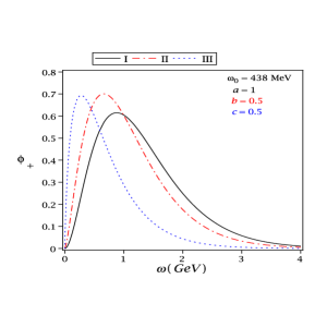
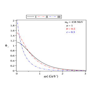
Figure 2: The dependence of $\varphi_{{}_{+}}(\omega)$ and $\varphi_{{}_{-}}(\omega)$ on $\omega$ for the three models.

Comparing to the two-particle DA’s, the contribution of the three-particle DA’s is less than $10\%$ in calculations of the form factors. The three-particle DA’s are related to a basis of DA’s such as $\phi_{3},\phi_{4},\psi_{4}$ and $\psi_{5}$ with definite twist, as follows JiMan :

$$\begin{aligned} \Psi_{{}_{A}}(\omega,\xi)&=\frac{1}{2}\,[\phi_{3}(\omega,\xi)+\phi_{4}(\omega,\xi)]\,,&\Psi_{{}_{V}}(\omega,\xi)&=\frac{1}{2}\,[-\phi_{3}(\omega,\xi)+\phi_{4}(\omega,\xi)]\,,\\ X_{{}_{A}}(\omega,\xi)&=\frac{1}{2}\,[-\phi_{3}(\omega,\xi)-\phi_{4}(\omega,\xi)+2\,\psi_{4}(\omega,\xi)]\,,&Y_{{}_{A}}(\omega,\xi)&=\frac{1}{2}\,[-\phi_{3}(\omega,\xi)-\phi_{4}(\omega,\xi)+\psi_{4}(\omega,\xi)-\psi_{5}(\omega,\xi)]\,.\end{aligned}$$ (25)

So far, several models have been proposed for the shape of $\phi_{3},\phi_{4},\psi_{4}$ and $\psi_{5}$. Since the structure of $\varphi_{{}_{+}}$ in three models in Eq. (23) is the exponential form, we choose the exponential model for the functions $\phi_{3},\phi_{4},\psi_{4}$ and $\psi_{5}$, presented as JiMan ; ShenWangWei :

$$\begin{aligned} \phi_{3}(\omega,\xi)&={\lambda_{E}^{2}-\lambda_{H}^{2}\over 6\,\omega_{0}^{5}}\,\omega\,\xi^{2}\,e^{-\frac{\omega+\xi}{\omega_{0}}}\,,&\phi_{4}(\omega,\xi)&={\lambda_{E}^{2}+\lambda_{H}^{2}\over 6\,\omega_{0}^{4}}\,\xi^{2}\,e^{-\frac{\omega+\xi}{\omega_{0}}}\,,\\ \psi_{4}(\omega,\xi)&={\lambda_{E}^{2}\over 3\,\omega_{0}^{4}}\,\omega\,\xi\,e^{-\frac{\omega+\xi}{\omega_{0}}}\,,&\psi_{5}(\omega,\xi)&=-{\lambda_{E}^{2}\over 3\,\omega_{0}^{3}}\,\xi\,e^{-\frac{\omega+\xi}{\omega_{0}}}\,.\end{aligned}$$ (26)

To analyze the form factors $f_{+}$, $f_{-}$, and $f_{T}$, the value of the Borel parameter $M^{2}$ must also be determined. The Borel parameter $M^{2}$ is not physical quantity, so the physical quantities, form factors, should be independent of it. The working region for $M^{2}$ is determined by requiring that the contributions of the higher states and continuum are effectively suppressed. The dependence of the form factors $f_{+}$, $f_{-}$ and $f_{T}$ on the Borel parameter $M^{2}$ is shown in Fig. 3, for the three models in $\omega_{0}=438\,\rm{MeV}$, and $q^{2}=0\,\rm{GeV^{2}}$.

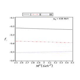
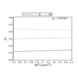
Figure 3: The dependence of the form factors $f_{+}$, $f_{-}$ and $f_{T}$ on the Borel parameter $M^{2}$ for the three models in $\omega_{0}=438\,\rm{MeV}$, and $q^{2}=0\,\rm{GeV^{2}}$.

This figure shows a good stability of the form factors with respect to the Borel parameter in the interval: $2.5\,\mbox{GeV}^{2}\leq M^{2}\leq 3.5\,\mbox{GeV}^{2}$. We take $M^{2}=3~{}\mbox{GeV}^{2}$ in our calculations. Uncertainties originated from the Borel parameter $M^{2}$ in this region, are about $5\%$.

Having all these input values and parameters, we proceed to carry out numerical calculations. Inserting the values of the masses, leptonic decay constants, continuum threshold, Borel mass, the parameters of the $B_{s}$-meson DA’s such as $\omega_{0}$ and other quantities that appear in the form factors in Eq. (II), we can calculate the form factors of the semileptonic $B_{s}\to K_{0}^{*}$ transitions at zero momentum transfer, $q^{2}=0\,\mbox{GeV}^{2}$. Table 1 shows central values of the form factors for the three models as well as sources of error and also uncertainties caused by them, separately. As can be seen $\omega_{0}$ and $f_{K_{0}^{*}}$ are the most significant sources of theory uncertainties.

Table 1: Central values of the form factors for the three models, as well as sources of error and also uncertainties of the form factors. The uncertainties $\Delta$ caused by the variations of the input parameters ($\delta{\omega_{0}}=\pm 0.150~{}\mbox{GeV}$, $\delta{f_{K_{0}^{*}}}=\pm 0.085~{}\mbox{GeV}$, $\delta{s_{0}}=\pm 0.4~{}\mbox{GeV}^{2}$, $\delta{m_{K_{0}^{*}}}=\pm 0.05~{}\mbox{GeV}$, $\delta{f_{B_{s}}}=\pm 0.001~{}\mbox{GeV}$, $\delta{\lambda_{E}^{2}}=\pm 0.01~{}\mbox{GeV}^{2}$, $\delta{\lambda_{H}^{2}}=\pm 0.05~{}\mbox{GeV}^{2}$, $\delta{M^{2}}=\pm 0.5~{}\mbox{GeV}^{2}$).

Model	Form Factor	Central Value	$\Delta(\omega_{0})$	$\Delta(f_{K_{0}^{*}})$	$\Delta(s_{0})$	$\Delta(m_{K_{0}^{*}})$	$\Delta(f_{B_{s}})$	$\Delta(\lambda_{E}^{2})$	$\Delta(\lambda_{H}^{2})$	$\Delta(M^{2})$
	$f_{+}(0)$	$+0.283$	${}^{+0.252}_{-0.114}$	${}^{+0.070}_{-0.047}$	${}^{+0.024}_{-0.027}$	${}^{+0.004}_{-0.003}$	${}^{+0.002}_{-0.003}$	${}^{+0.000}_{-0.000}$	${}^{+0.004}_{-0.004}$	${}^{+0.006}_{-0.007}$
I	$f_{-}(0)$	$-0.228$	${}^{+0.114}_{-0.262}$	${}^{+0.038}_{-0.056}$	${}^{+0.027}_{-0.024}$	${}^{+0.003}_{-0.003}$	${}^{+0.002}_{-0.002}$	${}^{+0.002}_{-0.002}$	${}^{+0.002}_{-0.001}$	${}^{+0.011}_{-0.008}$
	$f_{T}(0)$	$+0.324$	${}^{+0.326}_{-0.145}$	${}^{+0.080}_{-0.054}$	${}^{+0.030}_{-0.034}$	${}^{+0.007}_{-0.006}$	${}^{+0.003}_{-0.003}$	${}^{+0.000}_{-0.001}$	${}^{+0.001}_{-0.002}$	${}^{+0.009}_{-0.012}$
	$f_{+}(0)$	$+0.412$	${}^{+0.279}_{-0.145}$	${}^{+0.102}_{-0.069}$	${}^{+0.025}_{-0.030}$	${}^{+0.006}_{-0.005}$	${}^{+0.003}_{-0.004}$	${}^{+0.000}_{-0.000}$	${}^{+0.003}_{-0.004}$	${}^{+0.005}_{-0.005}$
II	$f_{-}(0)$	$-0.369$	${}^{+0.149}_{-0.293}$	${}^{+0.061}_{-0.092}$	${}^{+0.029}_{-0.027}$	${}^{+0.004}_{-0.006}$	${}^{+0.003}_{-0.004}$	${}^{+0.001}_{-0.001}$	${}^{+0.001}_{-0.002}$	${}^{+0.009}_{-0.009}$
	$f_{T}(0)$	$+0.495$	${}^{+0.363}_{-0.186}$	${}^{+0.123}_{-0.082}$	${}^{+0.033}_{-0.038}$	${}^{+0.011}_{-0.009}$	${}^{+0.004}_{-0.004}$	${}^{+0.001}_{-0.001}$	${}^{+0.002}_{-0.001}$	${}^{+0.009}_{-0.009}$
	$f_{+}(0)$	$+0.511$	${}^{+0.195}_{-0.124}$	${}^{+0.127}_{-0.085}$	${}^{+0.015}_{-0.018}$	${}^{+0.008}_{-0.005}$	${}^{+0.005}_{-0.004}$	${}^{+0.000}_{-0.000}$	${}^{+0.004}_{-0.003}$	${}^{+0.013}_{-0.007}$
III	$f_{-}(0)$	$-0.506$	${}^{+0.127}_{-0.188}$	${}^{+0.084}_{-0.125}$	${}^{+0.019}_{-0.014}$	${}^{+0.006}_{-0.007}$	${}^{+0.005}_{-0.004}$	${}^{+0.001}_{-0.001}$	${}^{+0.002}_{-0.001}$	${}^{+0.005}_{-0.008}$
	$f_{T}(0)$	$+0.644$	${}^{+0.243}_{-0.158}$	${}^{+0.161}_{-0.107}$	${}^{+0.019}_{-0.023}$	${}^{+0.014}_{-0.011}$	${}^{+0.006}_{-0.005}$	${}^{+0.001}_{-0.000}$	${}^{+0.002}_{-0.001}$	${}^{+0.013}_{-0.007}$

Taking into account all the uncertainty values except $\omega_{0}$, the numerical values of the form factors $f_{+}$, $f_{-}$ and $f_{T}$ in $q^{2}=0\,\mbox{GeV}^{2}$ are presented in Table 2 for the three models. This table also includes a comparison of our results with the predictions of other approaches such as the LCSR with the light-meson DA’s HanWuFu ; YMWang ; YJSun , perturbative QCD (PQCD) RHLi and QCDSR method MZYang ; Ghahramany . As can be seen, there is a very good agreement between our results in model II and predictions of the conventional LCSR with the light-meson DA’s in S2 YMWang . As a result, our calculations confirm scenario 2 for describing the scalar meson $K_{0}^{*}$.

Table 2: The form factors of the semileptonic $B_{s}\to K_{0}^{*}$ transitions at zero momentum transfer from the three models and different approaches.

Method	$f_{+}(0)$	$f_{-}(0)$	$f_{T}(0)$
(I)	${+0.28}^{+0.11}_{-0.09}$	${-0.10}^{+0.09}_{-0.19}$	${+0.32}^{+0.13}_{-0.11}$
This work    (II)	${+0.41}^{+0.14}_{-0.12}$	${-0.37}^{+0.11}_{-0.14}$	${+0.50}^{+0.18}_{-0.14}$
(III)	${+0.51}^{+0.16}_{-0.12}$	${-0.51}^{+0.12}_{-0.16}$	${+0.64}^{+0.22}_{-0.15}$
LCSR(S2)    YMWang	$+0.42^{+0.13}_{-0.08}$	$-0.34^{+0.10}_{-0.10}$	$+0.52^{+0.18}_{-0.08}$
LCSR(S2)    HanWuFu	$+0.39^{+0.04}_{-0.04}$	$-0.25^{+0.05}_{-0.05}$	$+0.41^{+0.04}_{-0.04}$
LCSR(S2)    YJSun	$+0.44$	$-0.44$	$--$
PQCD(S2)   RHLi	$+0.56^{+0.16}_{-0.13}$	$--$	$+0.72^{+0.27}_{-0.17}$
LCSR(S1)    YJSun	$+0.10$	$-0.10$	$--$
PQCD(S1)   RHLi	$-0.32^{+0.06}_{-0.07}$	$--$	$-0.41^{+0.08}_{-0.09}$
QCDSR        MZYang	$+0.24\pm 0.10$	$--$	$--$
QCDSR        Ghahramany	$+0.25\pm 0.05$	$-0.17\pm 0.04$	$+0.21\pm 0.04$

Due to the presence of cutoff in the QCD calculations, we look for a parametrization of the form factors to extend our results to the full physical region, $0\leq q^{2}\leq{(m_{B_{s}}-m_{K_{0}^{*}})}^{2}$. Through fitting the results of the LCSR among the region $0<q^{2}<8\,\rm{GeV}^{2}$, we extrapolate them with the pole model parametrization

$$f_{i}(q^{2})=\frac{f_{i}(0)}{1-\alpha(q^{2}/m_{B_{s}}^{2})+\beta{(q^{2}/m_{B_{s}}^{2})}^{2}},$$ (27)

with the constants $\alpha$ and $\beta$ determined from the fitting procedure. The values of the parameters $\alpha$ and $\beta$ are presented in Table 3 for the three models. The values of parameter $f_{i}(0)$ expressed the form factor results at $q^{2}=0\,\mbox{GeV}^{2}$ were listed in Table 2, before.

Table 3: The parameters $\alpha$ and $\beta$ obtained for the form factors of the semileptonic $B\to K_{0}^{*}$ transitions for the three models.

Form Factor	$f_{+}(q^{2})$				$f_{-}(q^{2})$				$f_{T}(q^{2})$
Model	I	II	III		I	II	III		I	II	III
$\alpha$	$-0.14$	$-0.24$	$-0.49$		$+0.09$	$+0.19$	$+0.46$		$-0.14$	$-0.27$	$-0.60$
$\beta$	$+0.26$	$+0.63$	$+3.89$		$-0.14$	$-0.45$	$-3.76$		$+0.25$	$+0.69$	$+5.00$

The dependence of the form factors $f_{+}$, $f_{-}$ and $f_{T}$ on $q^{2}$, for the three models, is shown in Fig. 4. In this work, the form factors are estimated in the LCSR approach up to the three-particle DA’s of the $B_{s}$-meson.

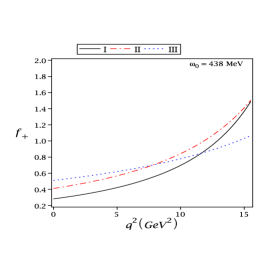
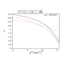
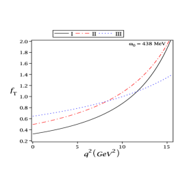
Figure 4: The dependence of the form factors $f_{+}(q^{2})$, $f_{-}(q^{2})$ and $f_{T}(q^{2})$ of the semileptonic $B_{s}\rightarrow K_{0}^{*}$ transitions on $q^{2}$ for the three models.

Our calculations show that the most contributions comes from the two-particle functions $\varphi_{\pm}$ for all form factors, so that the contributions of the three-particle DA’s are less than $10\%$ of the total. The contributions of the two- and three-particle DA’s in the form factors depict in Fig. 5 for model II, separately.

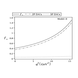
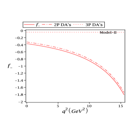
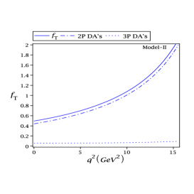
Figure 5: The contributions of the two-particle DA’s (2P DA’s) and three-particle DA’s (3P DA’s) in the form factors $f_{+}(q^{2})$, $f_{-}(q^{2})$ and $f_{T}(q^{2})$ for model II.

The form factors at large recoil should satisfy the following relations ColFazWan :

$$f_{T}(q^{2})=\frac{m_{B_{s}}+m_{K_{0}^{*}}}{m_{B_{s}}}f_{+}(q^{2})=-\frac{m_{b}}{m_{B_{s}}-m_{K_{0}^{*}}}f_{-}(q^{2}).$$ (28)

Figuer 6 shows that the computed form factors from the LCSR with the $B_{s}$-meson DA’s for the three models satisfy the relations in Eq. (28), by considering the errors.

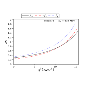
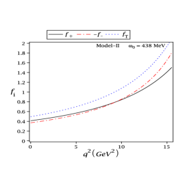
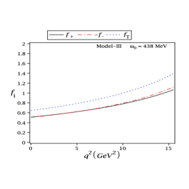
Figure 6: The dependence of the form factors $f_{+}(q^{2})$, $-f_{-}(q^{2})$ and $f_{T}(q^{2})$ on $q^{2}$ via the LCSR with the $B_{s}$-meson DA’s for the three models.

With the derived transition form factors, one can proceed to perform the calculations on some interesting observables in phenomenology, such as decay rate, polarization asymmetry, and forward-backward asymmetry. Note that the forward-backward asymmetry for the decay mode $B_{s}\to K_{0}^{*}l^{+}l^{-}$ is exactly equal to zero in the SM BelGen .

The effective Hamiltonian for $b\to ul\bar{\nu}_{l}$ transition is

$$\mathcal{H}_{\rm{eff}}(b\to ul\bar{\nu}_{l})=\frac{G_{F}}{\sqrt{2}}V_{ub}\,\bar{u}\gamma_{\mu}(1-\gamma_{5})b\,\,\bar{l}\gamma^{\mu}(1-\gamma_{5})\nu_{l}\,.$$ (29)

With this Hamiltonian, the $q^{2}$ dependant decay width $\frac{d\Gamma}{dq^{2}}$ can be expressed as YJSun

$$\frac{d\Gamma}{dq^{2}}(B_{s}\to K_{0}^{*}\,l\,\bar{\nu}_{l})=\frac{G_{F}^{2}|V_{ub}|^{2}}{384\,\pi^{3}\,m_{B_{s}}^{3}}\frac{(q^{2}-m_{l}^{2})^{2}}{(q^{2})^{3}}\sqrt{(m_{B_{s}}^{2}-m_{K_{0}^{*}}^{2}-q^{2})^{2}-4\,q^{2}\,m_{K_{0}^{*}}^{2}}\,\,\,\Big{\{}(m_{l}^{2}+2q^{2})$$

$$\times\sqrt{(m_{B_{s}}^{2}-m_{K_{0}^{*}}^{2}-q^{2})^{2}-4q^{2}m_{K_{0}^{*}}^{2}}\,\,f_{+}^{2}(q^{2})+3\,m_{l}^{2}\,(m_{B_{s}}^{2}-m_{K_{0}^{*}}^{2})^{2}\,\Big{[}f_{+}(q^{2})+\frac{q^{2}}{m_{B_{s}}^{2}-m_{K_{0}^{*}}^{2}}f_{-}(q^{2})\Big{]}^{2}\Big{\}},$$ (30)

where $V_{ub}=(3.82\pm 0.24)\times 10^{-3}$, and $m_{l}$ is the mass of the lepton. Integrating Eq. (III) over $q^{2}$ in the whole physical region $m_{l}^{2}\leq q^{2}\leq{(m_{B_{s}}-m_{K_{0}^{*}})}^{2},$ and using the total mean lifetime $\tau_{B_{s}}=(1.509\pm 0.004)~{}ps$ PDG , we present the branching ratio values of semileptonic decays $B_{s}\to K_{0}^{*}\,l\,\bar{\nu}_{l}$, ($l=\mu,\tau$) in Table 4, for the three models. Here, we should also stress that the results obtained for the electron are very close to the results of the muon, and for this reason, we only present the branching ratios for the muon in our table. This table contains the results estimated via the conventional LCSR with the light-meson DA’s YMWang and PQCD RHLi through S$2$ as well as QCDSR MZYang approaches. Considering the range of errors, the values obtained in this work are in a logical agreement with the LCSR and PQCD results. Especially, the obtained values of model II are in a good agreement with the conventional LCSR. As can be seen in this table, uncertainties in the values obtained for the branching ratios of the semileptonic decays $B_{s}\to K_{0}^{*}\,l\,\bar{\nu}_{l}$ are very large. The main source of errors comes from the form factor $f_{+}(q^{2})$.

Table 4: The branching ratio values of $B_{s}\to K_{0}^{*}\,l\,\bar{\nu}_{l}$ for the three models and different approaches.

Mode	This work			LCSR (S2) YMWang	PQCD (S2) RHLi	QCDSR MZYang
	I	II	III
$\mbox{Br}(B_{s}\to K_{0}^{*}\mu\,\nu_{\mu})\times 10^{4}$	$0.99^{+0.89}_{-0.37}$	$1.67^{+1.32}_{-0.53}$	$1.90^{+1.48}_{-0.63}$	$1.30^{+1.30}_{-0.40}$	$2.45^{+1.77}_{-1.05}$	$0.36^{+0.38}_{-0.24}$
$\mbox{Br}(B_{s}\to K_{0}^{*}\tau\,\nu_{\tau})\times 10^{4}$	$0.49^{+0.33}_{-0.17}$	$0.71^{+0.57}_{-0.26}$	$0.65^{+0.55}_{-0.24}$	$0.52^{+0.57}_{-0.18}$	$1.09^{+0.82}_{-0.47}$	$--$

We show the dependency of the differential branching ratios of $B_{s}\to K_{0}^{*}\,l\,\bar{\nu}_{l}$, ($l=\mu,\tau$) decays on $q^{2}$ for the three models in Fig. 7.

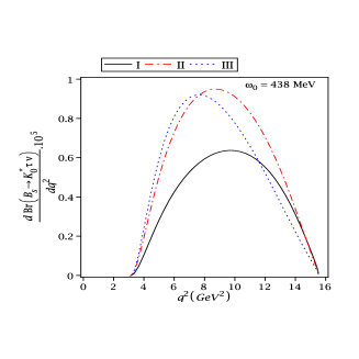
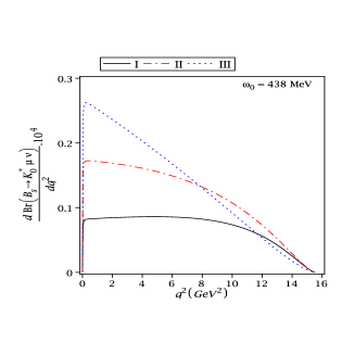
Figure 7: Differential branching ratios of the semileptonic $B\to K_{0}^{*}l\nu_{l}$ decays on $q^{2}$ for the three models.

The semileptonic decays $B_{s}\to K_{0}^{*}l^{+}l^{-}/\nu\bar{\nu}$ are induced by the FCNC (Appendix). Using the parametrization of these transitions in terms of the form factors, the differential decay width in the rest frame of $B_{s}$-meson can be written as:

$$\frac{d{\Gamma}}{dq^{2}}(B_{s}\rightarrow K_{0}^{*}{\nu}\bar{\nu}) = \frac{G_{F}^{2}{\mid}V_{td}V^{*}_{tb}{\mid}^{2}m_{B_{s}}^{3}\alpha^{2}}{2^{8}\pi^{5}}~{}\frac{{\mid}D_{\nu}(x_{t}){\mid}^{2}}{\rm{sin}^{4}\theta_{W}}~{}\phi^{3/2}(1,\hat{r},\hat{s}){\mid}f_{+}(q^{2}){\mid}^{2}~{},$$

$$\frac{d\Gamma}{dq^{2}}\left(B_{s}\rightarrow K_{0}^{*}l^{+}l^{-}\right) = \frac{G_{F}^{2}{\mid}V_{td}V^{*}_{tb}{\mid}^{2}m_{B_{s}}^{3}\alpha^{2}}{3\times 2^{9}\pi^{5}}v\,\phi^{1/2}(1,\hat{r},\hat{s})\left[\left(1+\frac{2\hat{l}}{\hat{s}}\right)\phi(1,\hat{r},\hat{s})\alpha_{1}+12~{}\hat{l}\beta_{1}\right],$$ (31)

where $\hat{r}$, $\hat{s}$, $\hat{l}$, $x_{t}$ and ${\hat{m}}_{b}$ and the functions $v$, $\phi(1,\hat{r},\hat{s})$, $D_{\nu}(x_{t})$, $\alpha_{1}$ and $\beta_{1}$ are defined as:

$$\hat{r}=\frac{m_{K_{0}^{*}}^{2}}{m_{B_{s}}^{2}}~{},\quad\quad\hat{s}=\frac{q^{2}}{m_{B_{s}}^{2}}~{},\quad\quad\hat{l}=\frac{m_{l}^{2}}{m_{B_{s}}^{2}}~{},\quad\quad x_{t}=\frac{m_{t}^{2}}{m_{W}^{2}}~{},\quad\quad{\hat{m}}_{b}=\frac{m_{b}}{m_{B_{s}}}~{},\quad\quad v=\sqrt{1-\frac{4\hat{l}}{\hat{s}}}~{},$$

$$D_{\nu}(x_{t})=\frac{x_{t}}{8}\Bigg{(}\frac{2+x_{t}}{x_{t}-1}+\frac{3x_{t}-6}{(x_{t}-1)^{2}}\ln x_{t}\Bigg{)}~{},\quad\quad\quad\quad{\phi}(1,\hat{r},\hat{s})=1+\hat{r}^{2}+\hat{s}^{2}-2\hat{r}-2\hat{s}-2\hat{r}\hat{s}~{},$$

$$\alpha_{1}=\biggl{|}C_{9}^{\rm eff}\,f_{+}(q^{2})+\frac{2\,{\hat{m}}_{b}\,C_{7}^{\rm eff}\,f_{T}(q^{2})}{1+\sqrt{\hat{r}}}\biggr{|}^{2}+|C_{10}f_{+}(q^{2})|^{2}~{},$$

$$\beta_{1}=|C_{10}|^{2}\biggl{[}\biggl{(}1+\hat{r}-{\hat{s}\over 2}\biggr{)}|f_{+}(q^{2})|^{2}+\biggl{(}1-\hat{r}\biggr{)}{\rm Re}(f_{+}(q^{2})f_{-}^{*}(q^{2}))+\frac{1}{2}\hat{s}|f_{-}(q^{2})|^{2}\biggr{]}.~{}$$ (32)

These expressions contain the Wilson coefficients $C^{\rm{eff}}_{7}=-0.313$, $C_{9}^{\rm{eff}}$ (see Appendix) and $C_{10}=-4.669$, the CKM matrix elements $|V_{td}V^{*}_{tb}|=0.008$, the form factors related to the fit functions, series of functions and constants. Integrating Eq. (III) over $q^{2}$ in the physical region $4m_{l}^{2}\leq q^{2}\leq{(m_{B_{s}}-m_{K_{0}^{*}})}^{2},$ and using $\tau_{B_{s}}$, the branching ratio results of the $B_{s}\rightarrow K_{0}^{*}l^{+}l^{-}/\nu\bar{\nu}$ are obtained for the three models as presented in Table 5. In this table, we show only the values obtained by considering the short distance (SD) effects contributing to the Wilson coefficient $C_{9}^{\rm eff}$ for charged lepton case. Predictions by the QCDSR Ghahramany , are smaller than those obtained in this work, because of their estimated form factors are smaller than ours (see Table 2).

Table 5: The branching ratios of the semileptonic $B_{s}\to K_{0}^{*}l^{+}l^{-}/\nu\bar{\nu}$ decays for the three models, including only the SD effects.

Mode	This work			QCDSRGhahramany
	I	II	III
$\mbox{Br}(B_{s}\to K_{0}^{*}\nu\bar{\nu})~{}~{}~{}~{}\times 10^{7}$	$0.98^{+0.55}_{-0.27}$	$1.66^{+0.95}_{-0.46}$	$1.89^{+1.07}_{-0.52}$	$0.25\pm 0.12$
$\mbox{Br}(B_{s}\to K_{0}^{*}\mu^{+}\mu^{-})\times 10^{8}$	$1.32^{+0.75}_{-0.36}$	$2.21^{+1.24}_{-0.62}$	$2.48^{+1.38}_{-0.69}$	$0.71\pm 0.29$
$\mbox{Br}(B_{s}\to K_{0}^{*}\tau^{+}\tau^{-})\times 10^{9}$	$0.61^{+0.34}_{-0.17}$	$0.63^{+0.35}_{-0.17}$	$0.45^{+0.25}_{-0.12}$	$0.35\pm 0.16$

It should be noted that we have computed the branching ratio values of $B_{s}\to K_{0}^{*}l^{+}l^{-}$ decays in the naive factorization approximation using the factorizable LO quark-loop, i.e., diagrams (a) and (b) in Fig. 8. In this method, contributions of the $O_{1-6}$ operators have the same form factor dependence as $C_{9}$ which can be absorbed into an effective Wilson coefficient $C^{\rm eff}_{9}$.

For a complete analysis of the branching ratio values of $B_{s}\to K_{0}^{*}l^{+}l^{-}$ decays at the LO, the contributions of the weak annihilation amplitude of diagram (c) must be added to the form factor amplitude related to diagrams (a) and (b) in Fig. 8.

Figure 8: Factorizable and nonfactorizable contributions in the LO. The circled cross marks the possible insertions of the virtual photon line.

Diagram (c) is related to the nonfactorizable effects at the LO. They arise from electromagnetic corrections to the matrix elements of purely hadronic operators in the weak effective Hamiltonian. Since the matrix elements of the semileptonic operators $O_{9,10}$ can be expressed through $B_{s}\to K_{0}^{*}$ form factors, nonfactorizable corrections contribute to the decay amplitude only through the production of a virtual photon, which then decays into the lepton pair LyZwi ; BenFelSei . These contributions for $B_{s}\to K_{0}^{*}(1430)$ decays are actually suppressed by small Wilson coefficients of the penguin operators and can therefore be neglected in the current analysis. In addition to the factorizable and nonfactorizable LO diagrams in Fig. 8, there are factorizable NLO quark-loop and nonfactorizable NLO hard-scattering and soft-gluon contributions in the FCNC $b\to s$ and $b\to d$ transitions and the effects of them must be taken into account KhodjRusov . Considering the large current uncertainties due to the form factors, the NLO effects can also be ignored in our calculations.

In this part, the branching ratios including LD effects are presented. In the range of $4m_{l}^{2}\leq q^{2}\leq(m_{B_{s}}-m_{K_{0}^{*}})^{2}$, there are two charm-resonances $J/\psi$ and $\psi(2S)$ used in our calculations. We introduce some cuts around the resonances of $J/\psi$ and $\psi(2S)$ and study the following three regions for muon:

$$\mbox{Region-1}: \ \ \ \ \ \ \ \ \sqrt{q^{2}_{min}}\;\leq\;\sqrt{q^{2}}\;\leq\;M_{J/\psi}-0.20,$$

$$\mbox{Region-2}: M_{J/\psi}+0.04\;\leq\;\sqrt{q^{2}}\;\leq\;M_{\psi(2S)}-0.10,$$

$$\mbox{Region-3}: \ \ M_{\psi(2S)}+0.02\;\leq\;\sqrt{q^{2}}\;\leq\;m_{B_{s}}-m_{K_{0}^{*}},$$ (33)

and for tau:

$$\mbox{Region-2}: \ \ \ \ \ \ \ \sqrt{q^{2}_{min}}\;\leq\;\sqrt{q^{2}}\;\leq\;M_{\psi(2S)}-0.02,$$

$$\mbox{Region-3}: M_{\psi(2S)}+0.02\;\leq\;\sqrt{q^{2}}\;\leq\;m_{B_{s}}-m_{K_{0}^{*}},$$ (34)

where $\sqrt{q^{2}_{min}}=2m_{l}$. The branching ratio values for muon and tau for the three models with LD effects are listed in Table 6.

Table 6: The branching ratios of the semileptonic $B_{s}\to K_{0}^{*}l^{+}l^{-}$ decays for the three models including LD effects.

Mode	Region-1				Region-2				Region-3				Total
	I	II	III		I	II	III		I	II	III		I	II	III
$\mbox{Br}(B_{s}\to K_{0}^{*}\mu^{+}\mu^{-})\times 10^{8}$	$0.94$	$1.73$	$2.14$		$0.20$	$0.27$	$0.21$		$0.02$	$0.02$	$0.01$		$1.16$	$2.02$	$2.36$
$\mbox{Br}(B_{s}\to K_{0}^{*}\tau^{+}\tau^{-})\times 10^{9}$	$--$	$--$	$--$		$0.21$	$0.24$	$0.17$		$0.31$	$0.30$	$0.22$		$0.52$	$0.54$	$0.39$

After numerical analysis, the dependency of the differential branching ratios for $B_{s}\to K_{0}^{*}l^{+}l^{-}/\nu\bar{\nu}$ on $q^{2}$ for model II, with and without LD effects is shown in Fig. 9.

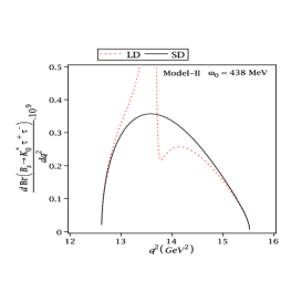
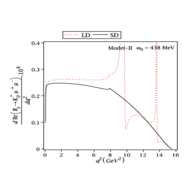
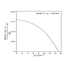
Figure 9: The differential branching ratios of the semileptonic $B_{s}\to K_{0}^{*}l^{+}l^{-}/\nu\bar{\nu}$ decays ($l=\mu,\tau$) on $q^{2}$ for model II. The solid and dotted lines show the results without and with the LD effects, respectively.

Finally, we want to calculate the longitudinal lepton polarization asymmetries for the considered decays. The longitudinal lepton polarization asymmetry formula for $B_{s}\to K_{0}^{*}l^{+}l^{-}$ is given as:

$$P_{L}=\frac{2v}{(1+\frac{2\hat{l}}{\hat{s}})\phi(1,\hat{r},\hat{s})\alpha_{1}+12\hat{l}\beta_{1}}{\rm{Re}}\left[\phi(1,\hat{r},\hat{s})\left(C_{9}^{eff}f_{+}(q^{2})-\frac{2C_{7}f_{T}(q^{2})}{1+\sqrt{\hat{r}}}\right)(C_{10}f_{+}(q^{2}))^{*}\right],$$ (35)

where $v,~{}\hat{l},~{}\hat{r},~{}\hat{s},~{}\phi(1,\hat{r},\hat{s}),\alpha_{1}$ and $\beta_{1}$ were defined before. The dependence of the longitudinal lepton polarization asymmetries for the $B_{s}\to K_{0}^{*}l^{+}l^{-},~{}(l=\mu,\tau)$ decays on the transferred momentum square $q^{2}$ for model II, with and without LD effects is plotted in Fig. 10.

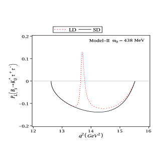
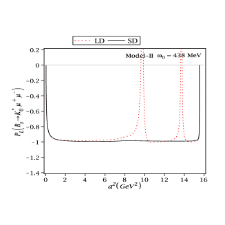
Figure 10: The dependence of the longitudinal lepton polarization asymmetries on $q^{2}$ for model II. The solid and dotted lines show the results without and with the LD effects, respectively.

The averaged values of the lepton polarization asymmetries of these decays for the three models, without the LD contributions are obtained and presented in Table 7. These polarization asymmetries provide valuable information on the flavor changing loop effects in the SM.

Table 7: Averaged values of the lepton polarization asymmetries of $B_{s}\to K_{0}^{*}l^{+}l^{-},~{}(l=\mu,\tau)$ decays for the three models, without the LD contributions.

Model	I	II	III
$\langle P_{L}\rangle_{\mu}$	$-0.80$	$-0.88$	$-0.98$
$\langle P_{L}\rangle_{\tau}$	$-0.12$	$-0.13$	$-0.11$

IV Conclusion

In summary, the transition form factors of the semileptonic $B_{s}\to K_{0}$ transitions were calculated via the LCSR with the $B_{s}$-meson DA’s in the $\rm SU(3)_{F}$ symmetry limit. We considered the three different models for the shapes of the two-particle DA’s, $\varphi_{\pm}$. It was shown that in estimation of the form factors, the main uncertainties came from the shape parameter $\omega_{0}$ and the decay constant of the $K_{0}^{*}$-meson. In this work, we used $\omega_{0}=\lambda_{B_{s}}$. Recently, the inverse moment of the $B_{s}$-meson distribution amplitude, $\lambda_{B_{s}}$ has been predicted from the QCDSR method as $\lambda_{B_{s}}=(438\pm 150)~{}\rm{MeV}$. There was a very good agreement between our results for the form factors at zero momentum transfer in model II and predictions of the conventional LCSR with the light-meson DA’s in scenario 2. Therefore, our calculations confirmed scenario 2 for describing the scalar meson $K_{0}^{*}(1430)$. Using the form factors $f_{+}(q^{2})$, $f_{-}(q^{2})$ and $f_{T}(q^{2})$, the branching ratio values for the semileptonic $B_{s}\to K_{0}^{*}l\bar{\nu_{l}}$ and $B_{s}\to K_{0}^{*}l\bar{l}/\nu\bar{\nu}$ ($l=e,\mu,\tau$) decays were calculated. It is worth mentioning that we computed the branching ratio values of $B_{s}\to K_{0}^{*}l^{+}l^{-}$ decays in the naive factorization approximation. Considering the SD and LD effects, the dependence of the differential branching ratios as well as the longitudinal lepton polarization asymmetries for $B_{s}\to K_{0}^{*}l\bar{l}$ decays were investigated with respect to $q^{2}$. Future experimental measurement can give valuable information about these aforesaid decays and the nature of the scalar meson $K_{0}^{*}(1430)$.

Appendix: The effective weak Hamiltonian of the $b\to d~{}l^{+}l^{-}$ transition

The effective weak Hamiltonian of the $b\to d~{}l^{+}l^{-}$ transition has the following form in the SM:

$$\mathcal{H}^{b\to d}_{\rm eff}=-\frac{G_{F}}{\sqrt{2}}\left(V_{ub}V_{ud}^{*}\sum_{i=1}^{2}C_{i}(\mu)O^{u}_{i}(\mu)+V_{cb}V_{cd}^{*}\sum_{i=1}^{2}C_{i}(\mu)O^{c}_{i}(\mu)-V_{tb}V_{td}^{*}\sum_{i=3}^{10}C_{i}(\mu)O_{i}(\mu)\right),$$

where $V_{jk}$ and $C_{i}(\mu)$ are the CKM matrix elements and Wilson coefficients, respectively. The local operators are current-current operators $O^{u,c}_{1,2}$, QCD penguin operators $O_{3-6}$, magnetic penguin operators $O_{7,8}$, and semileptonic electroweak penguin operators $O_{9,10}$. The explicit expressions of these operators for $b\to dl^{+}l^{-}$ transition are written as Buras0

$$\begin{array}[]{ll}O_{1}=(\bar{d}_{i}c_{j})_{V-A},(\bar{c}_{j}b_{i})_{V-A},&O_{2}=(\bar{d}c)_{V-A}(\bar{c}b)_{V-A},\\ O_{3}=(\bar{d}b)_{V-A}\sum_{q}(\bar{q}q)_{V-A},&O_{4}=(\bar{d}_{i}b_{j})_{V-A}\sum_{q}(\bar{q}_{j}q_{i})_{V-A},\\ O_{5}=(\bar{d}b)_{V-A}\sum_{q}(\bar{q}q)_{V+A},&O_{6}=(\bar{d}_{i}b_{j})_{V-A}\sum_{q}(\bar{q}_{j}q_{i})_{V+A},\\ O_{7}=\frac{e}{8\pi^{2}}m_{b}(\bar{d}\sigma^{\mu\nu}(1+\gamma_{5})b)F_{\mu\nu},&O_{8}=\frac{g}{8\pi^{2}}m_{b}(\bar{d}_{i}\sigma^{\mu\nu}(1+\gamma_{5}){T}_{ij}b_{j}){G}_{\mu\nu},\\ O_{9}=\frac{e}{8\pi^{2}}(\bar{d}b)_{V-A}(\bar{l}l)_{V},&O_{10}=\frac{e}{8\pi^{2}}(\bar{d}b)_{V-A}(\bar{l}l)_{A},\end{array}$$

where ${G}_{\mu\nu}$ and $F_{\mu\nu}$ are the gluon and photon field strengths, respectively; ${T}_{ij}$ are the generators of the $SU(3)$ color group; $i$ and $j$ denote color indices. Labels $(V\pm A)$ stand for $\gamma^{\mu}(1\pm\gamma^{5})$. The magnetic and electroweak penguin operators $O_{7}$, and $O_{9,10}$ are responsible for the SD effects in the FCNC $b\to d$ transition, but the operators $O_{1-6}$ involve both SD and LD contributions in this transition. In the naive factorization approximation, contributions of the $O_{1-6}$ operators have the same form factor dependence as $C_{9}$ which can be absorbed into an effective Wilson coefficient $C^{\rm eff}_{9}$. The effective Wilson coefficient $C_{9}^{\rm{eff}}$ includes both the SD and LD effects as

$$C^{\rm eff}_{9}=C_{9}+Y_{SD}(q^{2})+Y_{LD}(q^{2}),$$

where $Y_{SD}(q^{2})$ describes the SD contributions from four-quark operators far away from the resonance regions, which can be calculated reliably in perturbative theory as Buras0 ; Aliev0 :

$$Y_{SD}(q^{2}) = 0.138~{}\omega(s)+h(\hat{m_{c}},s)C_{0}+\lambda_{u}\,h(\hat{m_{c}},s)(3C_{1}+C_{2})-\frac{1}{2}h(1,s)(4C_{3}+4C_{4}+3C_{5}+C_{6})$$

$$- \frac{1}{2}h(0,s)(2\lambda_{u}[3C_{1}+C_{2}]+C_{3}+3C_{4})+\frac{2}{9}(3C_{3}+C_{4}+3C_{5}+C_{6}),$$

where $s=q^{2}/m_{b}^{2}$, $\hat{m_{c}}=m_{c}/m_{b}$, $C_{0}=3C_{1}+C_{2}+3C_{3}+C_{4}+3C_{5}+C_{6}$, $\lambda_{u}=\frac{V_{ub}V^{*}_{ud}}{V_{tb}V^{*}_{td}}$, and

$$\omega(s)=-\frac{2}{9}\pi^{2}-\frac{4}{3}{\rm Li}_{2}(s)-\frac{2}{3}\ln(s)\ln(1-s)-\frac{5+4s}{3(1+2s)}\ln(1-s)-\frac{2s(1+s)(1-2s)}{3(1-s)^{2}(1+2s)}\ln(s)+\frac{5+9s-6s^{2}}{3(1-s)(1+2s)},$$

represents the ${\cal O}(\alpha_{s})$ correction coming from one gluon exchange in the matrix element of the operator $O_{9}$ Jezabek , while $h(\hat{m}_{c},s)$ and $h(0,s)$ represent one-loop corrections to the four-quark operators $O_{1-6}$ Misiak . The functional form of the $h(\hat{m_{c}},s)$ and $h(0,s)$ are as:

$$h(\hat{m}_{c},s)=-\frac{8}{9}\ln\frac{m_{b}}{\mu}-\frac{8}{9}\ln\hat{m}_{c}+\frac{8}{27}+\frac{4}{9}x-\frac{2}{9}(2+x)|1-x|^{1/2}\left\{\begin{array}[]{ll}\left(\ln\left|\frac{\sqrt{1-x}+1}{\sqrt{1-x}-1}\right|-i\pi\right),&\mbox{for }x\equiv\frac{4\hat{m}_{c}^{2}}{s}<1\\ &\\ 2\arctan\frac{1}{\sqrt{x-1}},&\mbox{for }x\equiv\frac{4\hat{m}_{c}^{2}}{s}>1\end{array}\right.$$

and

$$h(0,s)=\frac{8}{27}-\frac{8}{9}\ln\frac{m_{b}}{\mu}-\frac{4}{9}\ln\ s+\frac{4}{9}i\pi\,.$$

The LD contributions, $Y_{LD}(q^{2})$ from four-quark operators near the $u\bar{u}$, $d\bar{d}$ and $c\bar{c}$ resonances cannot be calculated from the first principles of QCD and are usually parametrized in the form of a phenomenological Breit-Wigner formula as Buras0 ; Aliev0 :

$$Y_{LD}(q^{2}) = \frac{3\pi}{\alpha^{2}}\left\{\left(C_{0}+\lambda_{u}[3C_{1}+C_{2}]\right)\sum_{V_{i}=J/\psi,\psi(2S)}\frac{\Gamma(V_{i}\to l^{+}l^{-})m_{V_{i}}}{m_{V_{i}}^{2}-q^{2}-im_{V_{i}}\Gamma_{V_{i}}}\right\}.$$

In the range of $4m_{l}^{2}\leq q^{2}\leq(m_{B_{s}}-m_{K_{0}^{*}})^{2}$, there are two charm-resonances $J/\psi(3.097)$ and $\psi(3.686)$ used in our calculations.

References

(1)
J. Weinstein and N. Isgur, Phys. Rev. Lett. 48, 659 (1982);
Phys. Rev. D 27, 588 (1983); R. Kaminski, L. Lesniak, and J.
P. Maillet, Phys. Rev. D 50, 3145 (1994); G. Janssen, B. C.
Pearce, K. Holinde, and J. Speth, Phys. Rev. D 52, 2690
(1995); R. Kaminski, L. Lesniak, and B. Loiseau, Phys. Lett. B 413, 130 (1997); J. A. Oller and E. Oset, Nucl. Phys. A620,
438 (1997); M. P. Locher, V. E. Markushin, and H. Q. Zheng, Eur.
Phys. J. C 4, 317 (1998).
(2)
R. L. Jaffe, Phys. Rev. D 15, 267 (1977); N. N. Achasov and
V.V. Gubin, Phys. Rev. D 56, 4084 (1997); M. N. Achasov et
al., Phys. Lett. B 438, 441 (1998); D. Black, A. Fariborz, and
J. Schechter, Phys. Rev. D 61, 074001 (2000); R. L. Jaffe and
F. Wilczek, Phys. Rev. Lett. 91, 232003 (2003); L. Maiani, F.
Piccinini, A. D. Polosa, and V. Riquer, Phys. Rev. Lett. 93,
212002 (2004).
(3)
H. Y. Cheng, C. K. Chua, and K. C. Yang, Phys. Rev. D 73,
014017 (2006).
(4)
V. M. Belyaev, A. Khodjamirian, and R. Ruckl, Z. Phys. C 60,
349 (1993).
(5)
A. Ali, V. M. Braun, and H. Simma, Z. Phys. C 63, 437 (1994).
(6)
V. M. Belyaev, V. M. Braun, A. Khodjamirian, and R. Ruckl, Phys.
Rev. D 51, 6177 (1995).
(7)
A. Khodjamirian, R. Ruckl, S. Weinzierl, and O. I. Yakovlev, Phys.
Lett. B 410, 275 (1997).
(8)
P. Ball and V. M. Braun, Phys. Rev. D 58, 094016 (1998).
(9)
E. Bagan, P. Ball, and V. M. Braun, Phys. Lett. B 417, 154
(1998).
(10)
P. Ball, JHEP 9809, 005 (1998).
(11)
P. Ball and R. Zwicky, JHEP 0110, 019 (2001).
(12)
P. Ball and R. Zwicky, Phys. Rev. D 71, 014015 (2005).
(13)
A. Khodjamirian, T. Mannel, and N. Offen, Phys. Lett. B 620,
52 (2005).
(14)
A. Khodjamirian, T. Mannel, and N. Offen, Phys. Rev. D 75,
054013 (2007).
(15)
V. M. Braun and A. Khodjamirian, Phys. Lett. B 718, 1014
(2013).
(16)
V. M. Braun, Y. Ji, and A. N. Manashov, Phys. Rev. D 100,
014023 (2019).
(17)
A. M. Galda and M. Neubert, Phys. Rev. D 102, 071501 (2020).
(18)
W. Wang, Y. M. Wang, J. Xu, and S. Zhao, Phys. Rev. D 102,
011502 (2020).
(19)
S. Zhao and A. V. Radyushkin, Phys. Rev. D 103, 054022 (2021).
(20)
A. G. Grozin and M. Neubert, Phys. Rev. D 55, 272 (1997).
(21)
V. M. Braun, D. Yu. Ivanov, and G. P. Korchemsky, Phys. Rev. D 69, 034014 (2004).
(22)
S. D. Genon and C. T. Sachrajda, Nucl. Phys. B650, 356
(2003).
(23)
P. Ball and E. Kou, JHEP 0304, 029 (2003).
(24)
S. J. Lee and M. Neubert, Phys. Rev. D 72, 094028 (2005).
(25)
G. Bell, T. Feldmann, Y. M. Wang, and M. W. Y. Yip, JHEP 11,
191 (2013).
(26)
T. Feldmann, B. O. Lange, and Y. M. Wang, Phys. Rev. D 89,
114001 (2014).
(27)
Y. M. Wang and Y. L. Shen, Nucl. Phys. B898, 563 (2015).
(28)
M. Beneke, V. Braun, Y. Ji, and Y. B. Wei, JHEP 07, 154
(2018).
(29)
V. M. Braun, Y. Ji, and A. N. Manashov, JHEP 1905, 022(2017).
(30)
C. D. Lü, Y. L. Shen, Y. M. Wang, and Y. B. Wei, JHEP 1901, 024 (2019).
(31)
I. I. Balitsky and V. M. Braun, Nucl. Phys. B311, 541 (1989).
(32)
P. A. Zyla et al. (Particle Data Group), Prog. Theor. Exp. Phys.
2020, 083C01 (2020).
(33)
D. S. Du, J. W. Li, and M. Z. Yang, Phys. Lett. B 619, 105
(2005).
(34)
S. Aoki, Y. Aoki, D. Becirevic et al. (FLAG Review 2019), Eur. Phys.
J. C 80, 113 (2020).
(35)
M. Rahimi and M. Wald, Phys. Rev. D 104, 016027 (2021).
(36)
B. O. Lange and M. Neubert, Phys. Rev. Lett. 91, 102001
(2003).
(37)
M. Beneke and T. Feldmann, Nucl. Phys. B592, 3 (2001).
(38)
M. Beneke, G. Buchalla, M. Neubert, and C. T. Sachrajda, Nucl. Phys.
B591, 313 (2000).
(39)
T. Janowski, B. Pullin, and R. Zwicky, JHEP 12, 008 (2021).
(40)
A. Heller et al. (Belle Collaboration), Phys. Rev. D 91 112009
(2015).
(41)
A. Khodjamirian, R. Mandal, and T. Mannel, JHEP 10, 043
(2020).
(42)
Y. M. Wang, M. J. Aslam, and C. D. Lü, Phys. Rev. D 78,
014006 (2008).
(43)
H. Y. Han, X. G. Wu, H. B. Fu, Q. L. Zhang, and T. Zhong, Eur. Phys.
J. C 49, 78 (2013).
(44)
Y. J. Sun, Z. H. Li, and T. Huang, Phys. Rev. D 83, 025024
(2011).
(45)
R. H. Li, C. D. Lü, W. Wang, and X. X. Wang, Phys. Rev. D 79, 014013 (2009).
(46)
M. Z. Yang, Phys. Rev. D 73, 034027 (2006) [Erratum-ibid. D
73, 079901 (2006)].
(47)
N. Ghahramany and R. Khosravi, Phys. Rev. D 80, 016009 (2009).
(48)
P. Colangelo, F. D. Fazio, and W. Wang, Phys. Rev. D 81,
074001 (2010).
(49)
G. Belanger, C. Q. Geng, and P. Turcotte, Nucl. Phys. B390,
253 (1993).
(50)
J. Lyon and R. Zwicky, Phys. Rev. D 88, 094004 (2013).
(51)
M. Beneke, Th. Feldmann, and D. Seidel, Eur. Phys. J. C 41,
173 (2005).
(52)
A. Khodjamirian, T. Mannel, A. A. Pivovarov, and Y. M. Wang, JHEP
1009, 089 (2010); A. Khodjamirian, T. Mannel, and Y. M. Wang,
JHEP 02, 010 (2013); C. Hambrock, A. Khodjamirian, and A.
Rusov, Phys. Rev. D 92, 074020 (2015); A. Khodjamirian and A.
V. Rusov, JHEP 08, 112 (2017).
(53)
A. J. Buras and M. Muenz, Phys. Rev. D 52, 186 (1995).
(54)
T. M. Aliev, V. Bashiry, and M. Savci, Phys, Rev, D 72, 034031
(2005).
(55)
M. Jezabek and J. H. Kuhn, Nucl. Phys. B320, 20 (1989).