Kramers-Kronig Relations for Nonlinear Rheology: 1. General Expression and Implications

Abstract

The principle of causality leads to linear Kramers-Kronig relations (KKR) that relate the real and imaginary parts of the complex modulus $G^{*}$ through integral transforms. Using the multiple integral generalization of the Boltzmann superposition principle for nonlinear rheology, and the principle of causality, we derived nonlinear KKR, which relate the real and imaginary parts of the $n^{\text{th}}$ order complex modulus $G_{n}^{*}$. For $n$=3, we obtained nonlinear KKR for medium amplitude parallel superposition (MAPS) rheology. A special case of MAPS is medium amplitude oscillatory shear (MAOS); we obtained MAOS KKR for the third-harmonic MAOS modulus $G_{33}^{*}$; however, no such KKR exists for the first harmonic MAOS modulus $G_{31}^{*}$. We verified MAPS and MAOS KKR for the single mode Giesekus model. We also probed the sensitivity of MAOS KKR when the domain of integration is truncated to a finite frequency window. We found that that (i) inferring $G_{33}^{\prime\prime}$ from $G_{33}^{\prime}$ is more reliable than vice-versa, (ii) predictions over a particular frequency range require approximately an excess of one decade of data beyond the frequency range of prediction, and (iii) $G_{33}^{\prime}$ is particularly susceptible to errors at large frequencies.

I Introduction

In the linear viscoelastic (LVE) regime, soft materials are subjected to infinitesimal deformations so that the mechanical response may be probed without perturbing the equilibrium microstructure. Linear viscoelasticity is commonly examined using three types of experiments: (i) step strain, (ii) creep or step stress, and (iii) oscillatory strain. These experiments lead, respectively, to the linear response functions: (i) stress relaxation modulus $G(t)$, (ii) creep compliance $J(t)$, and (iii) complex modulus $G^{*}(\omega)$. Here, $t$ and $\omega$ represent time and frequency, respectively. These LVE response functions provide insights into material microstructure, and are part of standard rheological characterization [1, 2, 3, 4]. These response functions are interrelated. If complete knowledge of any one property is available, the remaining two can be inferred. The relaxation modulus $G(t)$ and creep compliance $J(t)$ are related to each other by the convolution relation. The complex modulus $G^{*}(\omega)$, on the other hand, is related to the Fourier transform of $G(t)$. The complex modulus has real and imaginary parts, $G^{*}(\omega)=G^{\prime}(\omega)+iG^{\prime\prime}(\omega)$, called the storage (or elastic) and loss (or viscous) modulus, respectively. These moduli are related to each other via Kramers-Kronig relations (KKR) [5, 6]. They can be experimentally measured by performing oscillatory shear (OS) experiments.

I.1 Linear Kramers-Kronig Relations

Suppose a material is subjected to an arbitrary time-dependent shear strain $\gamma(t)$. In the LVE regime, the induced shear stress $\sigma(t)$ is related to the deformation history by the Boltzmann superposition principle [2, 3, 4],

$$\sigma(t)=\int_{-\infty}^{t}G(t-t^{\prime})\dfrac{d\gamma(t^{\prime})}{dt^{\prime}}\,dt^{\prime},$$ (1)

where $t$ is the current time, and ${t}^{\prime}$ is the time associated with application of deformation field. The principle of causality stipulates that the relaxation modulus $G(t-t^{\prime})=0$ for $t-t^{\prime}<0$. Using this principle, the complex modulus can be related to the relaxation modulus via a modified Fourier transform,

$$G^{*}(\omega)=i\omega\int_{-\infty}^{\infty}G(t)\,e^{-i\omega t}\,dt=i\omega\int_{0}^{\infty}G(t)\,e^{-i\omega t}dt.$$ (2)

Note that the complex viscosity $\eta^{*}(\omega)=\eta^{\prime}(\omega)-i\eta^{\prime\prime}(\omega)=G^{*}(\omega)/(i\omega)$ and the relaxation modulus $G(t)$ form a standard Fourier transform pair.

Using the principle of causality again to write $G(t)$ as a sum of an even and odd function, it can be shown that [3, 4],

$$G(t)=\dfrac{2}{\pi}\int_{0}^{\infty}\dfrac{G^{\prime}(\omega)}{\omega}\sin\omega t\,d\omega=\dfrac{2}{\pi}\int_{0}^{\infty}\dfrac{G^{\prime\prime}(\omega)}{\omega}\cos\omega t\,d\omega.$$ (3)

This constrains the functional forms of $G^{\prime}(\omega)$ and $G^{\prime\prime}(\omega)$ to be even and odd functions of $\omega$, respectively. By manipulating equations 2 and 3, we obtain the linear KKR :

$$G^{\prime}(\omega) =-\dfrac{2\omega^{2}}{\pi}\int_{0}^{\infty}\dfrac{G^{\prime\prime}(u)/u}{u^{2}-\omega^{2}}du$$

$$G^{\prime\prime}(\omega) =\dfrac{2\omega}{\pi}\int_{0}^{\infty}\dfrac{G^{\prime}(u)}{u^{2}-\omega^{2}}du.$$ (4)

Since the integrals have a singularity at $u=\omega$, the Cauchy principal value of the integrals is implied. Originally, KKR were proposed for specific atomic systems using physical arguments [6, 8, 9], but subsequently generalized using complex analysis, and assumptions of linearity, causality, and analyticity [10, 11]. Indeed, KKR can be derived in a succinct form from the residue theorem in complex analysis with deceptive simplicity as [12],

$$\eta^{*}(\omega)=\dfrac{i}{\pi}\int_{-\infty}^{\infty}\dfrac{\eta^{*}(u)}{u-\omega}du.$$ (5)

This equation is equivalent to the two relations in equation 4. Table 1 summarizes different forms in which linear KKR can be expressed .

	Complex Form	Pair Form
modulus	$\dfrac{G^{*}(\omega)}{\omega}=\dfrac{i}{\pi}\int\limits_{-\infty}^{\infty}\dfrac{G^{*}(u)/u}{u-\omega}du.$	$G^{\prime}(\omega)=-\dfrac{2\omega^{2}}{\pi}\int\limits_{0}^{\infty}\dfrac{G^{\prime\prime}(u)/u}{u^{2}-\omega^{2}}du$
		$G^{\prime\prime}(\omega)=\dfrac{2\omega}{\pi}\int\limits_{0}^{\infty}\dfrac{G^{\prime}(u)}{u^{2}-\omega^{2}}du$
viscosity	$\eta^{*}(\omega)=\dfrac{i}{\pi}\int\limits_{-\infty}^{\infty}\dfrac{\eta^{*}(u)}{u-\omega}du.$	$\eta^{\prime}(\omega)=\dfrac{2}{\pi}\int\limits_{0}^{\infty}\dfrac{u\eta^{\prime\prime}(u)}{u^{2}-\omega^{2}}\,du$
		$\eta^{\prime\prime}(\omega)=\dfrac{2\omega}{\pi}\int\limits_{0}^{\infty}\dfrac{\eta^{\prime}(u)}{\omega^{2}-u^{2}}\,du$

Table 1: Different forms of linear Kramers-Kronig relations.

It is useful to emphasize that the relationship between the real and imaginary parts of $G^{*}(\omega)$ implied by KKR is underpinned by the principle of causality. It is merely a mathematical reflection of the physical constraint $G(t<0)=0$, mediated through the Fourier transform of a real causal function. Nevertheless, it can be practically useful. For example, in small amplitude oscillatory shear (SAOS) experiments a sinusoidal strain $\gamma(t)=\gamma_{0}\sin\omega t$ with amplitude $\gamma_{0}$ and angular frequency $\omega$ is applied [3, 14]. In the LVE limit, the stress response is given by,

$$\sigma(t)=\sigma_{\text{SAOS}}(t)=\gamma_{0}\left(G^{\prime}(\omega)\sin\omega t+G^{\prime\prime}(\omega)\cos\omega t\right).$$ (6)

Modern rheometers can measure this response, and infer $G^{\prime}(\omega)$ and $G^{\prime\prime}(\omega)$ over a range of frequencies in a typical frequency sweep experiment. For thermo-rheologically simple materials, this frequency range can be widened to several decades using the time-temperature superposition principle [3]. Manual shifting of individual datasets to produce master-curves of $G^{*}(\omega)$ can result in violation of KKR. Thus, KKR can be used for data-validation of experimentally measured $G^{*}(\omega)$ [15, 16].

I.2 MAOS and MAPS Rheology

In the LVE limit of $\gamma_{0}\rightarrow 0$, stresses induced in a material are small and harmonic. As the magnitude of the deformation is gradually increased, nonlinear viscoelastic features start to manifest, and the stress response becomes non-harmonic. In conventional large amplitude oscillatory shear (LAOS) experiments, an oscillatory strain field $\gamma(t)=\gamma_{0}\sin\omega t$ similar to SAOS experiments, is applied [17, 18, 19]. For large values of amplitude $\gamma_{0}$, higher nonlinear modes are activated, and the stress response is often represented by a power series [20],

$$\sigma(t)=\sum\limits_{n\in\text{odd}}^{\infty}\sigma_{n}(t)=\sum\limits_{n\in\text{odd}}^{\infty}\sum\limits_{m\in\text{odd}}^{n}\gamma_{0}^{n}\left[G_{nm}^{\prime}(\omega)\sin(m\omega t)+G_{nm}^{\prime\prime}(\omega)\cos(m\omega t)\right],$$ (7)

where the nonlinear complex moduli $G_{nm}^{*}(\omega)=G_{nm}^{\prime}(\omega)+iG_{nm}^{\prime\prime}(\omega)$ are functions of only frequency. The summations include only odd values of $m$ and $n$ due to the odd symmetry of shear stress with shear strain. In the medium amplitude oscillatory shear (MAOS) regime, only the weakest nonlinear modes are activated, and the stress response $\sigma(t)=\sigma_{1}(t)+\sigma_{3}(t)+\mathcal{O}(\gamma_{0}^{5})$ can be truncated after the leading nonlinear term $n=3$ in equation 7 as,

$$\sigma(t)= \gamma_{0}\left[G_{11}^{\prime}\sin\omega t+G_{11}^{\prime\prime}\cos\omega t\right]+$$

$$\gamma_{0}^{3}\left[G_{31}^{\prime}\sin\omega t+G_{31}^{\prime\prime}\cos\omega t+G_{33}^{\prime}\sin 3\omega t+G_{33}^{\prime\prime}\cos 3\omega t\right],$$ (8)

where $\sigma_{1}=\sigma_{\text{SAOS}}$ and the LVE complex modulus is given by $G^{*}=G_{11}^{\prime}+iG_{11}^{\prime\prime}$. The stress term $\sigma_{3}(t)$ associated with cubic power of strain is the MAOS contribution; the MAOS moduli associated with the first and third harmonic are $G^{*}_{31}=G^{\prime}_{31}+iG^{\prime\prime}_{31}$, and $G^{*}_{33}=G^{\prime}_{33}+iG^{\prime\prime}_{33}$, respectively. MAOS measurements have been used to discriminate between linear and branched polymers [21, 22, 23], evaluate nanoparticle dispersion quality [24, 25], droplet size dispersion in polymer blends [26, 27], quantify filler-matrix interactions in filled rubbers [28, 29] etc.

Experimentally, extraction of the MAOS moduli is indirect, and involves careful extrapolation. The effort and care required is significantly greater than that required in the measurement of LVE moduli $G^{\prime}(\omega)$ and $G^{\prime\prime}(\omega)$, in part, due to the narrow window of suitable strain amplitudes [30]. If $\gamma_{0}$ is too small, MAOS signals are too weak and difficult to measure. If $\gamma_{0}$ is too large, the stress response is contaminated by the contribution of modes higher than the third harmonic. Furthermore, the optimal range of $\gamma_{0}$ is frequency-dependent; at low frequencies, higher strain amplitudes are necessary to ferret out MAOS signatures. In practice, the stress response is measured at multiple strain-amplitudes in the target zone, and the “true” MAOS moduli are extracted by extrapolation. Due to the complicated process involved, validating experimental data before interpretation is paramount. The companion paper provides a method for efficiently accomplishing this task [31].

Medium amplitude parallel superposition (MAPS) can be seen as a generalization of the MAOS protocol [32]. Instead of the single-tone sinusoidal strain in MAOS, the strain waveform in MAPS consists of a superposition of three sine waves with frequencies $\omega_{1}$, $\omega_{2}$, and $\omega_{3}$,

$$\gamma_{\text{MAPS}}(t)=\gamma_{0}\left(\sin(\omega_{1}t)+\sin(\omega_{2}t)+\sin(\omega_{3}t)\right).$$ (9)

This perturbation elicits a much richer asymptotic nonlinear response than MAOS. Indeed, as introduced formally in section II it leads to a strain-independent third-order complex modulus $G_{3}^{*}(\omega_{1},\omega_{2},\omega_{3})$ which offers a complete characterization of the material’s asymptotic nonlinear behavior. By complete, we mean that using $G_{3}^{*}(\omega_{1},\omega_{2},\omega_{3})$ the nonlinear response to any arbitrary medium amplitude deformation history can be predicted via a generalization of Boltzmann superposition principle.

Therefore, MAOS can be thought of as a special, low-dimensional projection of MAPS: it can be shown that the MAOS moduli, $G_{31}^{*}$ and $G_{33}^{*}$, are special cases of the third order or MAPS modulus $G_{3}^{*}(\omega_{1},\omega_{2},\omega_{3})$ [32],

$$G_{31}^{*}(\omega) =\dfrac{3}{4}G_{3}^{*}(\omega,-\omega,\omega)$$

$$G_{33}^{*}(\omega) =-\dfrac{1}{4}G_{3}^{*}(\omega,\omega,\omega).$$ (10)

Due to experimental challenges, characterization of materials using MAPS has barely started [33, 34, 35]. Regardless, for the purposes of this work, MAPS provides a convenient general theoretical lens for interpreting MAOS measurements and KKR.

I.3 Organization

This paper is organized as follows: we begin with a generalization of the Boltzmann superposition principle to nonlinear rheology using a multiple integral expansion in section II. We highlight similarities and connections between higher-order terms and their LVE counterparts. We then mathematically derive a general nonlinear KKR (equation 24).

In section III, we narrow our focus by specializing these general KKR to MAPS and MAOS rheology. It turns out that for the MAOS modulus $G_{33}^{*}$ we can formulate a KKR (equation 29); unfortunately no such KKR exists for $G_{31}^{*}$. Finally, in section IV, we test KKR on the single mode Giesekus model for which the third-order complex modulus $G_{3}^{*}(\omega_{1},\omega_{2},\omega_{3})$ is analytically known. In particular, we verify that the MAPS moduli are consistent with the appropriate KKR. Finally, we explore the sensitivity of the MAOS KKR when the domain of integration is limited to a finite frequency window.

II Derivation of Kramers-Kronig Relations for Nonlinear Rheology

The Boltzmann superposition principle can be generalized to nonlinear rheology using a multiple integral expansion [36, 37, 38, 39, 32]. The general framework for stress induced due to imposed strain can be represented using an infinite Volterra series,

$$\sigma(t)=\sum_{n\in\text{odd}}^{\infty}\,\sigma_{n}(t),$$ (11)

where the summation includes only odd values of $n$ due to the odd symmetry between shear stress and strain, i.e, $\sigma(-\gamma)=-\sigma(\gamma)$. The contribution of the $n^{\text{th}}$ mode is given by,

$$\sigma_{n}(t)=\int_{-\infty}^{t}\cdots\int_{-\infty}^{t}G_{n}(t-t_{1},t-t_{2},\cdots,t-t_{n})\prod_{m=1}^{n}\dot{\gamma}(t_{m})\,dt_{m},$$ (12)

where $\dot{\gamma}(t)$ is the shear rate, and $G_{n}(t-t_{1},t-t_{2},\cdots,t-t_{n})$ is the $n^{\text{th}}$ order relaxation modulus that generalizes the linear relaxation modulus. The principle of causality stipulates that $G_{n}(t-t_{1},t-t_{2},\cdots,t-t_{n})=0$ if $t-t_{i}<0$ for any $i=1,2,\cdots,n$. The first term in this series,

$$\sigma_{1}=\int_{-\infty}^{t}G_{1}(t-t_{1})\,\dot{\gamma}(t_{1})dt_{1}$$ (13)

is identical to the Boltzmann superposition principle given by equation 1 with $G_{1}(t)\equiv G(t)$. Subsequent terms ($n\geq 3$) in equation 12 take into account stress induced due to the interaction of strains applied at different times $t_{i}$ and $t_{j}$. In LVE, such cross-effects are negligible.

Nonlinear effects in oscillatory shear flow can evaluated by taking a Fourier transform (denoted by “hat”) of equation 11,

$$\hat{\sigma}(\omega)=\sum_{n\in\text{odd}}^{\infty}\,\hat{\sigma}_{n}(\omega)=\sum_{n\in\text{odd}}^{\infty}\int_{-\infty}^{\infty}\sigma_{n}(t)\,e^{-i\omega t}dt$$ (14)

where the contribution of the $n^{\text{th}}$ mode is,

$$\hat{\sigma}_{n}(\omega)=\dfrac{1}{(2\pi)^{n-1}}\int_{-\infty}^{\infty}\overset{n}{\cdots}\,\int_{-\infty}^{\infty}G_{n}^{*}(\omega_{1},\ldots,\omega_{n})\,\delta\left(\omega-\sum_{m=1}^{n}\omega_{m}\right)\left(\prod_{m=1}^{n}\hat{\dot{\gamma}}(\omega_{m})\,d\omega_{m}\right).$$ (15)

The nonlinear complex relaxation modulus $G_{n}^{*}\left({\omega_{1}},{\omega_{2}},\ldots,{\omega_{n}}\right)$ is the modified Fourier transform of the nonlinear relaxation modulus $G_{n}(t_{1},\ldots,t_{n})$,

$$G_{n}^{*}(\omega_{1},\ldots,\omega_{n})=\left(\prod_{m=1}^{n}i\omega_{m}\right)\int_{0}^{\infty}\overset{n}{\cdots}\,\int_{0}^{\infty}G_{n}(t_{1},\cdots,t_{n})\left(\prod_{m=1}^{n}e^{-i\omega_{m}t_{m}}dt_{m}\right).$$ (16)

Note that the first term corresponding to $n=1$ is the usual linear complex modulus $G_{1}^{*}(\omega)=G^{*}(\omega)$ encountered in the LVE regime as equation 2. The next odd term corresponding to $n=3$, or $G_{3}^{*}(\omega_{1},\omega_{2},\omega_{3})$, represents the leading nonlinear term that can be experimentally characterized using MAPS rheology. Due to the Volterra representation, $G_{n}^{*}$ obeys permutation symmetry and is invariant with respect to the permutation of its arguments. Thus, for example, $G_{3}^{*}(\omega_{1},\omega_{2},\omega_{3})=G_{3}^{*}(\omega_{2},\omega_{1},\omega_{3})=G_{3}^{*}(\omega_{3},\omega_{2},\omega_{1})$, etc.

Analogous to the linear complex viscosity $\eta^{*}(\omega)=G^{*}(\omega)/(i\omega)$, it is convenient to introduce the $n^{\text{th}}$ order complex viscosity $\eta_{n}^{*}(\omega_{1},\cdots,\omega_{n})=\eta_{n}^{\prime}(\omega_{1},\cdots,\omega_{n})-i\eta_{n}^{\prime\prime}(\omega_{1},\cdots,\omega_{n})$, which is related to the $n^{\text{th}}$ order complex modulus $G_{n}^{*}$ via,

$$G_{n}^{*}(\omega_{1},\cdots,\omega_{n})=\left(\prod_{m=1}^{n}i\omega_{j}\right)\eta_{n}^{*}(\omega_{1},\cdots,\omega_{n}).$$ (17)

Using this definition, we can write equation 16 as,

$$\eta^{*}_{n}(\omega_{1},\cdots,\omega_{n})=\int_{0}^{\infty}\overset{n}{\cdots}\,\int_{0}^{\infty}G_{n}(t_{1},\cdots,t_{n})\left(\prod_{m=1}^{n}e^{-i\omega_{m}t_{m}}dt_{m}\right).$$ (18)

Now that we have defined all the relevant terms, we can begin deriving a general form of KKR following the approach of Hutchings et al. [40]. Let $u$ and $\omega$ denote arbitrary frequencies. Consider the following integral with $p_{i}\geq 0$ for all $i=1,\cdots,n$,

$$I=\int_{-\infty}^{\infty}\dfrac{\eta^{*}_{n}(\omega_{1}+p_{1}u,\cdots,\omega_{n}+p_{n}u)}{u-\omega}du$$ (19)

Substituting equation 18 for $\eta_{n}^{*}$,

$$I=\int_{-\infty}^{\infty}\int_{0}^{\infty}\overset{n}{\cdots}\,\int_{0}^{\infty}G_{n}(t_{1},\cdots,t_{n})\,e^{-i\sum\omega_{m}t_{m}}\cdot\dfrac{e^{-iu\sum p_{m}t_{m}}}{u-\omega}\,\left(\prod_{m=1}^{n}dt_{m}\right)du,$$ (20)

where the summations that occur as arguments to exponential functions, $\sum\omega_{m}t_{m}$ and $\sum p_{m}t_{m}$, run from $m=1$ to $n$. We can switch the order of integration to isolate terms that involve $u$ and obtain,

$$I=\int_{0}^{\infty}\overset{n}{\cdots}\,\int_{0}^{\infty}G_{n}(t_{1},\cdots,t_{n})\,e^{-i\sum\omega_{m}t_{m}}\left(\prod_{m=1}^{n}dt_{m}\right)\int_{-\infty}^{\infty}\dfrac{e^{-iu\sum p_{m}t_{m}}}{u-\omega}du$$ (21)

We can analytically compute the integral over $u$, by using the following result for constant $a\neq 0$,

$$\int_{-\infty}^{\infty}\dfrac{e^{-iua}}{u-\omega}du=(-i\pi)e^{-i\omega a}.$$ (22)

Using equation 22 in equation 21, and invoking equation 18 in the last step, we can show that,

$$I =(-i\pi)\int_{0}^{\infty}\overset{n}{\cdots}\,\int_{0}^{\infty}G_{n}(t_{1},\cdots,t_{n})e^{-i\sum\omega_{m}t_{m}}\cdot e^{-i\omega\sum p_{m}t_{m}}\left(\prod_{m=1}^{n}dt_{m}\right)$$

$$=(-i\pi)\int_{0}^{\infty}\overset{n}{\cdots}\,\int_{0}^{\infty}G_{n}(t_{1},\cdots,t_{n})e^{-i\sum(\omega_{m}+p_{m}\omega)t_{m}}\left(\prod_{m=1}^{n}dt_{m}\right)$$

$$=(-i\pi)\,\eta^{*}_{n}(\omega_{1}+p_{1}\omega,\cdots,\omega_{n}+p_{n}\omega).$$ (23)

We can equate the RHS of equations 19 and 23 to obtain a general form of nonlinear KKR,

$$\eta^{*}_{n}(\omega_{1}+p_{1}\omega,\cdots,\omega_{n}+p_{n}\omega)=\dfrac{i}{\pi}\int_{-\infty}^{\infty}\dfrac{\eta_{n}^{*}(\omega_{1}+p_{1}u,\cdots,\omega_{n}+p_{n}u)}{u-\omega}du.$$ (24)

Note that this relation holds when $p_{i}\geq 0$ for all $i=1,\cdots,n$, with at least one $p_{i}>0$, due to equation 22. This is the most general form of KKR for nonlinear rheology in this work. Several other useful forms are special cases of this relation. A particular special case is obtained by substituting $p_{j}=1$ and $p_{i}=0$ for all $i\neq j$ where $1\leq i,j\leq n$, $\omega_{j}=0$, $u=\omega_{j}^{\prime}$, and $\omega=\omega_{j}$,

$$\eta^{*}_{n}(\omega_{1},\cdots,\omega_{j},\cdots,\omega_{n})=\dfrac{i}{\pi}\int_{-\infty}^{\infty}\dfrac{\eta^{*}_{n}(\omega_{1},\cdots,\omega_{j}^{\prime},\cdots,\omega_{n})}{\omega_{j}^{\prime}-\omega_{j}}d\omega_{j}^{\prime}.$$ (25)

Note that the RHS involves integrating over the $j^{\text{th}}$ input frequency. For $n=1$, the correspondence with the linear KKR in equation 5 is obvious. We can obtain an equivalent form in terms of higher order complex modulus by using equation 17,

$$\dfrac{G^{*}_{n}(\omega_{1},\cdots,\omega_{j},\cdots,\omega_{n})}{\omega_{j}}=\dfrac{i}{\pi}\int_{-\infty}^{\infty}\dfrac{G^{*}_{n}(\omega_{1},\cdots,\omega_{j}^{\prime},\cdots,\omega_{n})/\omega_{j}^{\prime}}{\omega_{j}^{\prime}-\omega_{j}}d\omega_{j}^{\prime}.$$ (26)

III Kramers-Kronig Relations for MAPS and MAOS

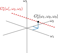
Figure 1: KKR for MAPS relates the third-order modulus at a point (black circle) to an integral over the first input frequency ($\omega_{1}^{\prime}$) (see equation 27) illustrated by the dashed red line.

We can specialize the general forms of KKR derived for nonlinear rheology (equations 24 - 26) for MAPS and MAOS experiments. For MAPS, two useful forms follow directly from equations 25 and 26 with $n=3$, and (say) $j=2$:

$$\eta^{*}_{3}(\omega_{1},\omega_{2},\omega_{3}) =\dfrac{i}{\pi}\int_{-\infty}^{\infty}\dfrac{\eta^{*}_{3}(\omega_{1},\omega_{2}^{\prime},\omega_{3})}{\omega_{2}^{\prime}-\omega_{2}}d\omega_{2}^{\prime}.$$

$$\dfrac{G^{*}_{3}(\omega_{1},\omega_{2},\omega_{3})}{\omega_{2}} =\dfrac{i}{\pi}\int_{-\infty}^{\infty}\dfrac{G^{*}_{3}(\omega_{1},\omega_{2}^{\prime},\omega_{3})/\omega_{j}^{\prime}}{\omega_{2}^{\prime}-\omega_{2}}d\omega_{2}^{\prime}.$$ (27)

For concreteness, the RHS of the equations above involve integrating over the second input frequency. Due to permutation symmetry, equivalent relations can also be furnished for first and third input frequencies. Figure 1 illustrates this relation for the case where the integral is expressed over the first input frequency. This family of KKR is useful for validating MAPS experiments where $G_{3}^{*}(\omega_{1},\omega_{2},\omega_{3})$ or $\eta_{3}^{*}(\omega_{1},\omega_{2},\omega_{3})$ is available.

III.1 KKR for MAOS

We can manipulate the general KKR relation (equation 24) to develop KKR that are useful for relating the real and imaginary parts of the MAOS moduli $G_{33}^{*}$, where the perturbation is single-tone. With $n=3$, we set $\omega_{1}=\omega_{2}=\omega_{3}=0$, and $p_{1}=p_{2}=p_{3}=1$ to obtain,

$$\eta^{*}_{3}(\omega,\omega,\omega)=\dfrac{i}{\pi}\int_{-\infty}^{\infty}\dfrac{\eta^{*}_{3}(u,u,u)}{u-\omega}du.$$ (28)

Using equation 10 and 17, we can rewrite the corresponding KKR in terms of the modulus,

$$G_{33}^{*}(\omega)=\dfrac{i}{\pi}\omega^{3}\int_{-\infty}^{\infty}\dfrac{1}{u^{3}}\dfrac{G_{33}^{*}(u)}{u-\omega}du.$$ (29)

We can equate the real and imaginary parts separately to obtain a pair of KKR relations. Using $G_{33}^{\prime}(-\omega)=G_{33}^{\prime}(\omega)$ and $G_{33}^{\prime\prime}(-\omega)=-G_{33}^{\prime\prime}(\omega)$, we can express these KKR for MAOS moduli $G_{33}^{*}$ on a non-negative frequency domain similar to the linear KKR as,

$$G_{33}^{\prime}(\omega) =-\dfrac{2\omega^{4}}{\pi}\int_{0}^{\infty}\dfrac{1}{u^{3}}\dfrac{G_{33}^{\prime\prime}(u)}{\left(u^{2}-\omega^{2}\right)}du$$

$$G_{33}^{\prime\prime}(\omega) =\dfrac{2\omega^{3}}{\pi}\int_{0}^{\infty}\dfrac{1}{{{u}^{2}}}\dfrac{G_{33}^{\prime}(u)}{\left(u^{2}-\omega^{2}\right)}du.$$ (30)

Just like linear KKR, these MAOS KKR can be used for numerically evaluating one signal from the other, or for data validation. Similar relations for the third-harmonic are widely used in nonlinear optics [40, 41, 42].

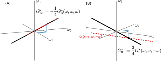
Figure 2: Schematic diagram illustrating KKR MAOS within the context of MAPS: (A) for $G_{33}^{*}$, application of KKR at a point (blue co-ordinates) involves an integral (dashed red line) that coincides with $G_{33}^{*}$ at all frequencies; (B) for $G_{31}^{*}$ the corresponding integral involves a quantity (dashed red line) that does not coincide with $G_{31}^{*}$.

Interestingly, while we can write specific expressions relating the real and and imaginary parts of $G_{33}^{*}(\omega)$ (equation 30), MAOS KKR relating the real and imaginary parts of $G_{31}^{*}(\omega)$ do not exist. In equation 24, since $p_{i}\geq 0$, the integrand on the RHS cannot be expressed as $\eta^{*}_{3}(u,u,-u)$, which is equal to $\eta_{31}^{*}(u)$. However, by using $p_{1}=1,p_{2}=0,p_{3}=0$ and $\omega_{1}=0,\omega_{2}=\omega,\omega_{3}=-\omega$, we obtain $\eta^{*}_{3}(u,\omega,-\omega)$ with two fixed input frequencies in the integrand, leading to:

$$\eta_{31}^{*}(\omega) =\eta_{3}^{*}(\omega,\omega,-\omega)=\dfrac{i}{\pi}\int\limits_{-\infty}^{\infty}\dfrac{\eta_{3}^{*}(u,\omega,-\omega)}{u-\omega}du$$

$$G_{31}^{*}(\omega) =G_{3}^{*}(\omega,\omega,-\omega)=\dfrac{i\omega}{\pi}\int\limits_{-\infty}^{\infty}\dfrac{G_{3}^{*}(u,\omega,-\omega)/u}{u-\omega}du.$$ (31)

The same expression can also be obtained by using $\omega_{1}=\omega$ and $\omega_{3}=-\omega$ in equation 27. This is the closest we can approach a KKR involving the MAOS modulus $G_{31}^{*}(\omega)$. This situation arises because MAOS moduli are a projection or subspace of the MAPS modulus $G_{3}^{*}(\omega_{1},\omega_{2},\omega_{3})$. As illustrated in figure 2, the MAOS moduli can be visualized as two particular diagonal vectors (marked by black lines) in the three-dimensional domain of $G_{3}^{*}$. For $G_{33}^{*}$, the integrand of the corresponding KKR relation (equation 30) lives in the same subspace shown by the dashed red line in figure 2A. Unfortunately, the integrand of equation 31 shown by the dashed red line in figure 2B lives in a different subspace and does not yield a KKR.

general nonlinear KKR
$\eta^{*}_{n}(\omega_{1}+p_{1}\omega,\cdots,\omega_{n}+p_{n}\omega)=\dfrac{i}{\pi}\int\limits_{-\infty}^{\infty}\dfrac{\eta_{n}^{*}(\omega_{1}+p_{1}u,\cdots,\omega_{n}+p_{n}u)}{u-\omega}du,\quad p_{i}\geq 0$
general	$\eta_{n}^{*}$	$\eta^{*}_{n}(\omega_{1},\cdots,\omega_{j},\cdots,\omega_{n})=\dfrac{i}{\pi}\int\limits_{-\infty}^{\infty}\dfrac{\eta^{*}_{n}(\omega_{1},\cdots,\omega_{j}^{\prime},\cdots,\omega_{n})}{\omega_{j}^{\prime}-\omega_{j}}d\omega_{j}^{\prime}$
	$G_{n}^{*}$	$\dfrac{G^{*}_{n}(\omega_{1},\cdots,\omega_{j},\cdots,\omega_{n})}{\omega_{j}}=\dfrac{i}{\pi}\int\limits_{-\infty}^{\infty}\dfrac{G^{*}_{n}(\omega_{1},\cdots,\omega_{j}^{\prime},\cdots,\omega_{n})/\omega_{j}^{\prime}}{\omega_{j}^{\prime}-\omega_{j}}d\omega_{j}^{\prime}$
MAPS	$\eta_{3}^{*}$	$\eta^{*}_{3}(\omega_{1},\omega_{2},\omega_{3})=\dfrac{i}{\pi}\int\limits_{-\infty}^{\infty}\dfrac{\eta^{*}_{3}(\omega_{1},\omega_{2}^{\prime},\omega_{3})}{\omega_{2}^{\prime}-\omega_{2}}d\omega_{2}^{\prime}$
	$G_{3}^{*}$	$\dfrac{G^{*}_{3}(\omega_{1},\omega_{2},\omega_{3})}{\omega_{2}}=\dfrac{i}{\pi}\int\limits_{-\infty}^{\infty}\dfrac{G^{*}_{3}(\omega_{1},\omega_{2}^{\prime},\omega_{3})/\omega_{j}^{\prime}}{\omega_{2}^{\prime}-\omega_{2}}d\omega_{2}^{\prime}$
MAOS	$\eta_{33}^{*}$	$\eta_{33}^{*}(\omega)=\dfrac{i}{\pi}\int\limits_{-\infty}^{\infty}\dfrac{\eta_{33}^{*}(u)}{u-\omega}du$
	$G_{33}^{*}$	$G_{33}^{*}(\omega)=\dfrac{i}{\pi}\omega^{3}\int\limits_{-\infty}^{\infty}\dfrac{1}{u^{3}}\dfrac{G_{33}^{*}(u)}{u-\omega}du$

Table 2: Summary of nonlinear KKR for general ($n^{\text{th}}$ order), MAPS and MAOS (third order) complex moduli. These equations can be derived from the general nonlinear KKR listed at the top of the table, which is derived in section II.

IV Validation of KKR for MAPS and MAOS

The various KKR expressions developed hitherto are tabulated in Table 2 for convenience. In this section, we verify the KKR expressions corresponding to the MAPS (equation 27) and MAOS moduli (equations 30 and 31) for the single mode Giesekus model. For this model, analytical expressions for the MAPS and MAOS moduli are available in the literature [32, 43, 44].

IV.1 KKR for MAPS

The single mode Giesekus model has three parameters, the two linear parameters: modulus $G_{0}$, and the relaxation time $\tau_{0}$, and the nonlinear parameter $\alpha_{G}$. The zero shear viscosity is related to the linear parameters via $\eta_{0}=G_{0}\tau_{0}$. Lennon et al. [32] derived the third-order complex modulus for various constitutive equations including the single mode Giesekus model, which can be written as,

$$\dfrac{\eta_{3}^{*}(\omega_{1},\omega_{2},\omega_{3})}{\eta_{0}\tau_{0}^{2}}=\dfrac{\alpha_{G}\left((3-2\alpha_{G})+i\sum\limits_{j}{{z_{j}}}\right)}{3\left(\prod\limits_{j}{\left(1+iz_{j}\right)}\right)}\dfrac{\left[-3-4i\sum\limits_{j}z_{j}+\sum\limits_{j}z_{j}^{2}+3\sum\limits_{j}\left(\prod\limits_{k\neq j}z_{k}\right)\right]}{\left[\prod\limits_{j}\left(1+i\sum\limits_{k\neq j}{{z_{k}}}\right)\right]\left(1+i\sum\limits_{j}z_{j}\right)},$$ (32)

using the dimensionless frequency $z_{i}=\omega_{i}\tau_{0}$, with $i=1,2,3$, for brevity. To validate the MAPS KKR (equation 27), we consider the integral,

$$\dfrac{1}{\eta_{0}\tau_{0}^{2}}\int_{-\infty}^{\infty}\dfrac{\eta_{3}^{*}\left(\omega_{1},u,\omega_{3}\right)}{\left(u-{\omega_{2}}\right)} du=\int_{-\infty}^{\infty}\dfrac{\alpha_{G}}{3(z-z_{2})}\dfrac{\left(3-2\alpha_{G}\right)+i\left({z_{1}}+z+{z_{3}}\right)}{\left(1+iz_{1}\right)\left(1+iz\right)\left(1+iz_{3}\right)}\times$$

$$\dfrac{-3-4i(z_{1}+z+z_{3})+\left(z_{1}^{2}+{{z}^{2}}+z_{3}^{2}\right)+3\left(z_{1}z+zz_{3}+z_{3}z_{1}\right)}{\left(1+i\left(z_{1}+z\right)\right)\left(1+i\left(z+z_{3}\right)\right)\left(1+i\left(z_{3}+z_{1}\right)\right)\left(1+i\left(z_{1}+z+z_{3}\right)\right)}dz,$$ (33)

where $z=\tau_{0}u$. This integral over $z$ can be evaluated analytically. As expected from the MAPS KKR equation 27, it leads to original expression for $\eta_{3}^{*}(\omega_{1},\omega_{2},\omega_{3})$ given by equation 32 with the appropriate prefactors. It is perhaps useful to point out that in trying to verify the MAPS KKR, a small typo was discovered in equation 61 and D8 of ref. [32] (the authors reported missing a factor of $i$ in the numerator of the first term on the RHS, which is fixed in equation 32). Note that verification of the MAPS KKR automatically validates equation 31 for $\eta_{31}^{*}$, which, as alluded to before, is strictly not a KKR as it does not relate the real and imaginary parts of the same property through an integral transform.

It is known that for inelastic constitutive equations such as generalized Newtonian fluids, the linear elastic moduli at all frequencies is ${G}^{\prime}=0$. Consequently, generalized Newtonian fluids do not obey the Fourier transform relation between $G^{\prime\prime}(\omega)$ and $G(t)$ given by equation 2. They violate the principle of causality, and even linear KKR given by equation 5 do not apply. For a generalized Newtonian fluid $\eta_{3}^{*}({\omega_{1}},{\omega_{2}},{\omega_{3}})=\eta^{\prime}(0)$ = constant [32]. For this case, we get $\int_{-\infty}^{\infty}\eta_{3}^{*}\left({\omega_{1}},u,{\omega_{3}}\right)/\left(u-{\omega_{2}}\right)du=0$, and hence MAPS KKR does not hold either. This result is expected because a generalized Newtonian fluid is an idealization; no real fluid demonstrates $G^{\prime}(\omega)=0$ at all frequencies.

IV.2 KKR for MAOS: Finite Frequency Window

Unlike $\eta_{31}^{*}$, the real and imaginary parts of $\eta_{33}^{*}$ are related through a KKR (equation 28). As with $\eta_{31}^{*}$, the validity of the corresponding specialized KKR is automatically implied by the validity of the MAPS KKR. MAOS KKR (equation 30) may can also be directly verified using the relations for $G_{33}^{*}$ derived by Gurnon and Wagner [43], and Bharadwaj and Ewoldt [44]. We obtain the same expressions from the MAPS relation (equation 32) using $\omega_{1}=\omega_{2}=\omega_{3}=\omega$,

$$\dfrac{G_{33}^{\prime}(\omega)}{G_{0}}=-\dfrac{1}{4}\dfrac{G_{3}^{\prime}(\omega,\omega,\omega)}{G_{0}} =\dfrac{\alpha_{G}z^{4}(-21+30z^{2}+51z^{4}+4\alpha_{G}(4-17z^{2}+3z^{4}))}{4(1+z^{2})^{3}(1+4z^{2})(1+9z^{2})}$$

$$\dfrac{G_{33}^{\prime\prime}(z)}{G_{0}}=-\dfrac{1}{4}\dfrac{G_{3}^{\prime\prime}(\omega,\omega,\omega)}{G_{0}} =\dfrac{\alpha_{G}z^{3}(-3+48z^{2}+33z^{4}-18z^{6}+\alpha_{G}(2-48z^{2}+46z^{4}))}{4(1+z^{2})^{3}(1+4z^{2})(1+9z^{2})},$$ (34)

with $z=\omega\tau_{0}$. Note that there is a small typo in Bharadwaj and Ewoldt [44] in the expression for $G_{33}^{\prime}$ where the term $+30z^{2}$ in the numerator is accidentally replaced by $-30z^{2}$.

Note that MAOS KKR require knowledge of $G_{33}^{*}$ over an infinite frequency window. In what follows, we explore the sensitivity of MAOS KKR when experimental data are available only over a limited frequency range, $\omega_{\min}\leq u\leq\omega_{\max}$. We denote these approximations of MAOS KKR by decorating the corresponding moduli with a tilde,

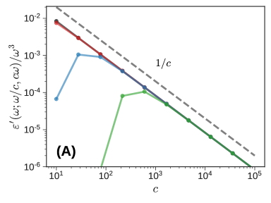
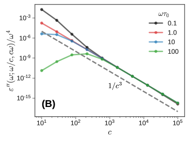
Figure 3: Normalized errors for finite-frequency approximations of MAOS KKR for the single mode Giesekus model with $G_{0}=\tau_{0}=1$ and $\alpha_{G}=0.2$: (A) $\varepsilon_{33}^{\prime}/\omega^{3}$ and (B) $\varepsilon_{33}^{\prime\prime}/\omega^{3}$ are plotted as a function of the parameter $c$, which controls the width of the frequency window via $\omega_{\min}=\omega/c$ and $\omega_{\max}=c\omega$. Four different values of the frequency $\omega\tau_{0}$ are selected. When the low frequency correction dominates the error, we expect $\varepsilon_{33}^{\prime}\propto\omega^{3}/c$ and $\varepsilon_{33}^{\prime\prime}\propto\omega^{4}/c^{3}$, which are indicated by the dashed gray lines.

$$\tilde{G}_{33}^{\prime}(\omega) =-\dfrac{2\omega^{4}}{\pi}\int_{\omega_{\min}}^{\omega_{\max}}\dfrac{1}{u^{3}}\dfrac{G_{33}^{\prime\prime}(u)}{\left(u^{2}-\omega^{2}\right)}du$$

$$\tilde{G}_{33}^{\prime\prime}(\omega) =\dfrac{2\omega^{3}}{\pi}\int_{\omega_{\min}}^{\omega_{\max}}\dfrac{1}{{{u}^{2}}}\dfrac{G_{33}^{\prime}(u)}{\left(u^{2}-\omega^{2}\right)}du.$$ (35)

Fortunately, these integrals can be evaluated analytically for the Giesekus model, although the resulting expressions are somewhat elaborate. We can define the absolute error between the true and approximate moduli to quantify the sensitivity of KKR to truncation of the frequency window as,

$$\epsilon_{33}^{\prime}(\omega;\omega_{\min},\omega_{\max}) =\left|G_{33}^{\prime}(\omega)-\tilde{G}_{33}^{\prime}(\omega;\omega_{\min},\omega_{\max})\right|$$

$$\epsilon_{33}^{\prime\prime}(\omega;\omega_{\min},\omega_{\max}) =\left|G_{33}^{\prime\prime}(\omega)-\tilde{G}_{33}^{\prime\prime}(\omega;\omega_{\min},\omega_{\max})\right|.$$ (36)

The error due to truncation has contributions from the left, $u\in[0,\omega_{\min}]$, and right, $u\in[\omega_{\max},\infty]$, tails. At large frequencies $u\rightarrow\infty$, the integrands of both the MAOS KKR decay rapidly as $1/u^{6}$,

$$\lim_{u\rightarrow\infty}\dfrac{1}{u^{3}}\dfrac{G_{33}^{\prime\prime}(u)}{\left(u^{2}-\omega^{2}\right)}\propto\dfrac{1}{u^{6}},\quad\lim_{u\rightarrow\infty}\dfrac{1}{{{u}^{2}}}\dfrac{G_{33}^{\prime}(u)}{\left(u^{2}-\omega^{2}\right)}\propto\dfrac{1}{u^{6}}.$$ (37)

Thus, the typical correction due to truncation of the high frequency or right tail is relatively modest compared to the truncation of the left tail, which we consider next. At low frequencies,

$$\lim_{u\rightarrow 0}\dfrac{1}{u^{3}}\dfrac{G_{33}^{\prime\prime}(u)}{\left(u^{2}-\omega^{2}\right)}\propto\dfrac{u^{0}}{\omega^{2}},\quad\lim_{u\rightarrow 0}\dfrac{1}{{{u}^{2}}}\dfrac{G_{33}^{\prime}(u)}{\left(u^{2}-\omega^{2}\right)}\propto\dfrac{u^{2}}{\omega^{2}}.$$ (38)

This left tail contribution to the error in equation 36 can be approximated as,

$$\epsilon_{33}^{\prime}(\omega;\omega_{\min},\infty) =-\dfrac{2\omega^{4}}{\pi}\int_{0}^{\omega_{\min}}\dfrac{1}{u^{3}}\dfrac{G_{33}^{\prime\prime}(u)}{\left(u^{2}-\omega^{2}\right)}du\approx-\dfrac{2\omega^{4}}{\pi}\int_{0}^{\omega_{\min}}\dfrac{u^{0}}{\omega^{2}}du\propto\omega^{2}\omega_{\min}$$

$$\epsilon_{33}^{\prime\prime}(\omega;\omega_{\min},\infty) =\dfrac{2\omega^{3}}{\pi}\int_{0}^{\omega_{\min}}\dfrac{1}{u^{2}}\dfrac{G_{33}^{\prime}(u)}{\left(u^{2}-\omega^{2}\right)}du\approx\dfrac{2\omega^{3}}{\pi}\int_{0}^{\omega_{\min}}\dfrac{u^{2}}{\omega^{2}}du\propto\omega\omega_{\min}^{3}.$$ (39)

Figure 3 depicts the total truncation error (equation 36) at four different frequencies $\omega\tau_{0}=$ 0.1, 1, 10, and 100 as a function of the width of the frequency window, which is controlled by the parameter $c$. We set $\omega_{\min}=\omega/c$ and $\omega_{\max}=c\omega$ for each choice of $\omega$ and $c$. As $c\rightarrow\infty$, the frequency window becomes infinite, and the errors $\varepsilon_{33}^{\prime}$ and $\varepsilon_{33}^{\prime\prime}$ go to zero. Error analysis (equation 39), which assumes that the left tail is primarily responsible suggests, $\varepsilon_{33}^{\prime}\propto\omega^{2}(\omega/c)=\omega^{3}/c$. This is clearly evident in figure 3A at sufficiently large $c$, where the $1/c$ dependence is shown by the dashed line, and the error is normalized by $\omega^{3}$. Similar analysis suggests that $\varepsilon_{33}^{\prime\prime}\propto\omega(\omega/c)^{3}=\omega^{4}/c^{3}$, which is also evident at large $c$ in figure 3B.

At smaller values of $c$ deviations from the asymptotic trendlines are visible. These deviations surface when the finite frequency window $[\omega/c,c\omega]$ does not include a sufficient information around the characteristic relaxation time of the Giesekus model, $\tau_{0}$. That is, it is important for the finite frequency window to include sufficient information around the corresponding characteristic frequency, i.e. $\omega_{\min}\ll 2\pi/\tau_{0}\ll\omega_{\max}$. The dataseries corresponding to for $\omega\tau_{0}=1$ always includes this region for the range of $c$ explored in 3. Thus, it tracks the asymptotic trendline more faithfully than other frequencies.

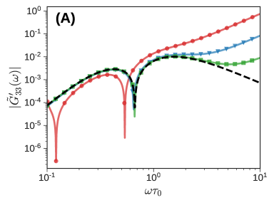
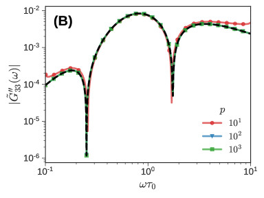
Figure 4: Finite-frequency window approximations of the third harmonic MAOS moduli $\tilde{G}_{33}^{\prime}(\omega)$ and $\tilde{G}_{33}^{\prime\prime}(\omega)$ for the single mode Giesekus model with $G_{0}=\tau_{0}=1$ and $\alpha_{G}=0.2$. Three different widths of the frequency window where $\omega_{\min}\tau_{0}=1/p$ and $\omega_{\max}\tau_{0}=p$ are shown. The dashed black lines are the true MAOS moduli.

Two other practical observations can be made from the figure: (i) at a given $\omega$ and $c$, the magnitude of the error $\varepsilon_{33}^{\prime\prime}$ is smaller, often much smaller, than the corresponding error $\varepsilon_{33}^{\prime}$, and (ii) for a fixed but sufficiently large frequency window, both errors increase rapidly with frequency $\omega$. This suggests that limiting the frequency window adversely affects high frequency predictions of $\tilde{G}_{33}^{\prime}(\omega)$ and $\tilde{G}_{33}^{\prime\prime}(\omega)$.

In practice, standard rheometers have a fixed frequency range, typically between $10^{-3}$ to $10^{3}$ rad/s. Hence, we can explore the sensitivity of $\tilde{G}_{33}^{\prime}(\omega)$ and $\tilde{G}_{33}^{\prime\prime}(\omega)$, when the experimental data are available from a fixed frequency window $\omega_{\min}=1/p$ and $\omega_{\max}=p$. Figure 4 shows $\tilde{G}_{33}^{\prime}(\omega)$ for $\omega\tau_{0}\in[0.1,10]$, at three different values of $p$ = 10, 100, and 1000.

As expected, the agreement between the approximate and true moduli improves as $p$ increases. Note that when $p=10$, the prediction, particularly for $\tilde{G}_{33}^{\prime}(\omega)$, is poor. The corresponding prediction for $\tilde{G}_{33}^{\prime\prime}(\omega)$ is not quite as bad. This seems to be a general trend: predictions of $G_{33}^{\prime\prime}(\omega)$ using MAOS KKR on limited frequency data for $G_{33}^{\prime}(\omega)$ are far more reliable than vice versa. This was foreshadowed by figure 3B, where the error $\varepsilon^{\prime\prime}<\varepsilon^{\prime}$ at the same value of $\omega$ and $c$.

However, even for $G_{33}^{\prime\prime}(\omega)$ we need data approximately one order of magnitude larger ($p=100$ corresponds to $\omega_{\min}=10^{-2}$ and $\omega_{\max}=10^{2}$) than the range of reliable prediction ($\omega\tau_{0}\in[0.1,10]$) shown in figure 4B. Increasing $p$ by another order of magnitude to 1000, results only in minor improvements in prediction of $G_{33}^{\prime\prime}(\omega)$. Unlike $G_{33}^{\prime\prime}(\omega)$, the predictions of $\tilde{G}_{33}^{\prime}(\omega)$ at high frequency, even at $p=1000$ are quite poor. This is anticipated by equation 39, which suggested that the error for the storage modulus is proportional to $\omega^{2}/p$, unlike the loss modulus which is proportional to $\omega/p^{3}$ and much better behaved.

V Summary

Linear KKR are integral transforms that relate the real and imaginary parts of the complex modulus $G^{*}$ (or complex viscosity $\eta^{*}$). These relations are a mathematical reflection of the principle of causality which constrains the linear relaxation modulus ($G(t<0)=0$). We started with a multiple integral expansion that generalizes the Boltzmann superposition principle to nonlinear rheology. Nonlinear KKR, similar to their linear counterparts, arises from the principle of causality which also constrains $n^{\text{th}}$ order relaxation modulus $G_{n}(t_{1},\cdots,t_{n})$.

We derived a general form of nonlinear KKR (equation 24) following the approach of Hutchings et al. [40]. We specialized this general KKR to MAPS rheology which relates the real and imaginary parts of the third-order complex modulus $G_{3}^{*}(\omega_{1},\omega_{2},\omega_{3})$ or complex viscosity $\eta_{3}^{*}(\omega_{1},\omega_{2},\omega_{3})$ (equation 27). Recall that knowledge of $G_{3}^{*}(\omega_{1},\omega_{2},\omega_{3})$ allows us to predict the asymptotically nonlinear material response to any arbitrary medium amplitude deformation history. MAOS rheology can then be considered as a popular special case of MAPS rheology that is characterized by two moduli $G_{31}^{*}=(3/4)G_{3}^{*}(\omega,-\omega,\omega)$ and $G_{33}^{*}=(-1/4)G_{3}^{*}(\omega,\omega,\omega)$. While a MAOS KKR relating the real and imaginary parts of $G_{33}^{*}$ can be written, no such expression relating the the real and imaginary parts of $G_{31}^{*}$ exists.

We verified the MAPS KKR relations on the single mode Giesekus model for which the third-order complex modulus $G_{3}^{*}(\omega_{1},\omega_{2},\omega_{3})$ is analytically known. With practical applications in mind, we investigated the sensitivity of the MAOS KKR when the domain of integration is truncated and data is limited to a finite frequency window. We found that: (i) the truncation error is typically dominated by the low-frequency or left tail, (ii) inferring $G_{33}^{\prime\prime}$ from $G_{33}^{\prime}$ is more reliable than vice versa, (iii) making predictions over a particular frequency range requires approximately an extra decade of data beyond the frequency range of prediction, and (iv) predictions of $G_{33}^{\prime}$ at large frequencies are poor, even when two decades of data beyond the prediction range are available.

Data Availability Statement

Data that support the findings of this study are available from the corresponding author upon reasonable request.

References

• Pipkin [1972] A. C. Pipkin, Lectures on viscoelasticity theory (Springer-Verlag, New York, NY, 1972).
• Tschoegl [1989] N. W. Tschoegl, The phenomenological theory of linear viscoelastic behavior: An introduction$1^{\text{st}}$ ed. (Springer-Verlag, Munich, Germany, 1989).
• Ferry [1980] J. D. Ferry, Viscoelastic properties of polymers$3^{\text{rd}}$ ed. (John Wiley & Sons, New York, NY, 1980).
• Cho [2016] K. S. Cho, Viscoelasticity of Polymers: Theory and Numerical Algorithms (Springer, Dordrecht, the Netherlands, 2016).
• Kramers [1929] H. Kramers, Die dispersion und absorption von röntgenstrahlen, Phys. Z 30, 522 (1929).
• de L. Kronig [1926] R. de L. Kronig, On the theory of dispersion of X-rays, J. Opt. Soc. Am. 12, 547 (1926).
• Note [1] For convenience and brevity, we assume that $G^{\prime}(0)=0$ (viscoelastic liquids), in this work. Generalizations of KKR to include nonzero equilibrium modulus $G^{\prime}(0)\not=0$ are straightforward.
• Kramers [1927] H. A. Kramers, La diffusion de la lumiere par les atomes, in Atti Cong. Intern. Fisica, Como, Vol. 2 (1927) pp. 545–557.
• Bohren [2010] C. F. Bohren, What did Kramers and Kronig do and how did they do it?, Eur. J. Phys. 31, 573 (2010).
• Toll [1956] J. S. Toll, Causality and the dispersion relation: Logical foundations, Phys. Rev. 104, 1760 (1956).
• King [2006] F. W. King, Alternative approach to the derivation of dispersion relations for optical constants, J. Phys. A: Math. Gen. 39, 10427 (2006).
• Hu [1989] B. Y. Hu, Kramers-Kronig in two lines, Am. J. Phys 57, 821 (1989).
• Note [2] Note that $\eta^{*}(\omega)$ is analogous to susceptibility $\chi(\omega)$ in optics. However, unlike $\eta^{*}=\eta^{\prime}-i\eta^{\prime\prime}$, susceptibility is defined as $\chi^{*}=\chi^{\prime}+i\chi^{\prime\prime}$. This difference in definition results in the comparable KKR, χ(ω)=1/(iπ)\ilimits@χ(u)uω𝑑u.superscript𝜒𝜔1𝑖𝜋superscriptsubscript\ilimits@superscript𝜒𝑢𝑢𝜔differential-d𝑢\chi^{*}(\omega)=1/(i\pi)\intop\ilimits@_{-\infty}^{\infty}\genfrac{}{}{}{0}{\chi^{*}(u)}{u-\omega}du..
• Dealy and Plazek [2009] J. Dealy and D. Plazek, Time-temperature superposition – a users guide, Rheol. Bull 78, 16 (2009).
• Winter [1997] H. Winter, Analysis of dynamic mechanical data: inversion into a relaxation time spectrum and consistency check, J. Non-Newtonian Fluid Mech. 68, 225 (1997), papers presented at the Polymer Melt Rheology Conference.
• Rouleau et al. [2013] L. Rouleau, J.-F. Deü, A. Legay, and F. Le Lay, Application of Kramers-Kronig relations to time-temperature superposition for viscoelastic materials, Mech. Mater. 65, 66 (2013).
• Tee and Dealy [1975] T. Tee and J. M. Dealy, Nonlinear viscoelasticity of polymer melts, Trans. Soc. Rheol. 19, 595 (1975).
• Giacomin and Dealy [1998] A. J. Giacomin and J. M. Dealy, Using large-amplitude oscillatory shear, in Rheological Measurement, edited by A. A. Collyer and D. W. Clegg (Springer Netherlands, Dordrecht, 1998) pp. 327–356.
• Hyun et al. [2011] K. Hyun, M. Wilhelm, C. O. Klein, K. S. Cho, J. G. Nam, K. H. Ahn, S. J. Lee, R. H. Ewoldt, and G. H. McKinley, A review of nonlinear oscillatory shear tests: Analysis and application of large amplitude oscillatory shear (LAOS), Prog. Polym. Sci. 36, 1697 (2011).
• Pearson and Rochefort [1982] D. S. Pearson and W. E. Rochefort, Behavior of concentrated polystyrene solutions in large-amplitude oscillating shear fields, J. Polym. Sci. Polym. Phys. 20, 83 (1982).
• Hyun and Wilhelm [2009] K. Hyun and M. Wilhelm, Establishing a new mechanical nonlinear coefficient Q from FT-rheology: First investigation of entangled linear and comb polymer model systems, Macromolecules 42, 411 (2009).
• Wagner et al. [2011] M. H. Wagner, V. H. Rolón-Garrido, K. Hyun, and M. Wilhelm, Analysis of medium amplitude oscillatory shear data of entangled linear and model comb polymers, J. Rheol. 55, 495 (2011).
• Song et al. [2016] H. Y. Song, O. S. Nnyigide, R. Salehiyan, and K. Hyun, Investigation of nonlinear rheological behavior of linear and 3-arm star 1,4-cis-polyisoprene (PI) under medium amplitude oscillatory shear (MAOS) flow via FT-rheology, Polymer 104, 268 (2016), rheology.
• Lee et al. [2016] S. H. Lee, H. Y. Song, and K. Hyun, Effects of silica nanoparticles on copper nanowire dispersions in aqueous pva solutions, Korea Aust. Rheol. J. 28, 111 (2016).
• Lim et al. [2013] H. T. Lim, K. H. Ahn, J. S. Hong, and K. Hyun, Nonlinear viscoelasticity of polymer nanocomposites under large amplitude oscillatory shear flow, J. Rheol. 57, 767 (2013).
• Ock et al. [2016] H. G. Ock, K. H. Ahn, S. J. Lee, and K. Hyun, Characterization of compatibilizing effect of organoclay in poly(lactic acid) and natural rubber blends by FT-rheology, Macromolecules 49, 2832 (2016).
• Salehiyan et al. [2014] R. Salehiyan, Y. Yoo, W. J. Choi, and K. Hyun, Characterization of morphologies of compatibilized polypropylene/polystyrene blends with nanoparticles via nonlinear rheological properties from FT-rheology, Macromolecules 47, 4066 (2014).
• Xiong and Wang [2018] W. Xiong and X. Wang, Linear-nonlinear dichotomy of rheological responses in particle-filled polymer melts, J. Rheol. 62, 171 (2018).
• Wang [1998] M.-J. Wang, Effect of polymer-filler and filler-filler interactions on dynamic properties of filled vulcanizates, Rubber Chem. Technol. 71, 520 (1998).
• Ewoldt and Bharadwaj [2013] R. H. Ewoldt and N. A. Bharadwaj, Low-dimensional intrinsic material functions for nonlinear viscoelasticity, Rheol. Acta 52, 201 (2013).
• Shanbhag and Joshi [2022] S. Shanbhag and Y. M. Joshi, Kramers-Kronig relations for nonlinear rheology: 2. Validation of medium amplitude oscillatory shear (MAOS) measurements (2022).
• Lennon et al. [2020a] K. R. Lennon, G. H. McKinley, and J. W. Swan, Medium amplitude parallel superposition (MAPS) rheology. Part 1: Mathematical framework and theoretical examples, J. Rheol. 64, 551 (2020a).
• Lennon et al. [2020b] K. R. Lennon, M. Geri, G. H. McKinley, and J. W. Swan, Medium amplitude parallel superposition (maps) rheology. Part 2: Experimental protocols and data analysis, J. Rheol. 64, 1263 (2020b).
• Lennon et al. [2021a] K. R. Lennon, G. H. McKinley, and J. W. Swan, The medium amplitude response of nonlinear Maxwell-Oldroyd type models in simple shear, J. Non-Newtonian Fluid Mech. 295, 104601 (2021a).
• Lennon et al. [2021b] K. R. Lennon, G. H. McKinley, and J. W. Swan, Medium amplitude parallel superposition (MAPS) rheology of a wormlike micellar solution, Rheol. Acta 60, 729 (2021b).
• Volterra [1959] V. Volterra, Theory of Functionals and of Integral and Integro-Differential Equations (Dover, New York, 1959).
• Bierwirth et al. [2019] S. P. Bierwirth, G. Honorio, C. Gainaru, and R. Böhmer, First-order and third-order nonlinearities from medium-amplitude oscillatory shearing of hydrogen-bonded polymers and other viscoelastic materials, Macromolecules 52, 8690 (2019).
• Findley et al. [1976] W. N. Findley, J. S. Lai, and K. Onaran, Chapter 7 - multiple integral representation, in Creep and Relaxation of Nonlinear Viscoelastic Materials, North-Holland Series in Applied Mathematics and Mechanics, Vol. 18 (North-Holland, 1976) pp. 131–175.
• Davis and Macosko [1978] W. M. Davis and C. W. Macosko, Nonlinear dynamic mechanical moduli for polycarbonate and pmma, J. Rheol. 22, 53 (1978).
• Hutchings et al. [1992] D. C. Hutchings, M. Sheik-Bahae, D. J. Hagan, and E. W. Van Stryland, Kramers-Krönig relations in nonlinear optics, Optical and Quantum Electronics 24, 1 (1992).
• Peiponen et al. [2004] K.-E. Peiponen, V. Lucarini, J. J. Saarinen, and E. Vartiainen, Kramers-Kronig relations and sum rules in nonlinear optical spectroscopy, Appl. Spectrosc. 58, 499 (2004).
• Boyd [2008] R. W. Boyd, Chapter 1: The nonlinear optical susceptibility, in Nonlinear Optics, edited by R. W. Boyd (Academic Press, Burlington, 2008) third edition ed., pp. 1–67.
• Kate Gurnon and Wagner [2012] A. Kate Gurnon and N. J. Wagner, Large amplitude oscillatory shear (LAOS) measurements to obtain constitutive equation model parameters: Giesekus model of banding and nonbanding wormlike micelles, J. Rheol. 56, 333 (2012).
• Bharadwaj and Ewoldt [2015] N. A. Bharadwaj and R. H. Ewoldt, Constitutive model fingerprints in medium-amplitude oscillatory shear, J. Rheol. 59, 557 (2015).