Chaos in the three-site Bose-Hubbard model — classical vs quantum

Abstract

We consider a quantum many-body system — the Bose-Hubbard system on three sites — which has a classical limit, and which is neither strongly chaotic nor integrable but rather shows a mixture of the two types of behavior. We compare quantum measures of chaos (eigenvalue statistics and eigenvector structure) in the quantum system, with classical measures of chaos (Lyapunov exponents) in the corresponding classical system. As a function of energy and interaction strength, we demonstrate a strong overall correspondence between the two cases. In contrast to both strongly chaotic and integrable systems, the largest Lyapunov exponent is shown to be a multi-valued function of energy.

I Introduction and Overview

How to translate classical chaos to quantum systems has been studied since the very beginning of quantum mechanics [1]. Classical chaos is the sensitivity of dynamics to initial perturbations [2], while quantum chaos manifests itself in various quantum properties, such as in level spacing distributions [3, 4, 5]. Level spacings of quantum models with an integrable classical limit typically follow Poisson’s law [6], while level spacings of models with a classically chaotic limit typically obey Wigner distributions [7, 8] typical of random matrices. In this work we will address the question how classical chaos relates to quantum notions of chaos in a many-body system that is neither integrable nor strongly chaotic, but rather shows a mixture of both behaviors, i.e., is a “mixed” system.

Regular and chaotic motion coexist in the phase space of mixed classical Hamiltonian systems, and corresponding quantum systems show a combination of chaotic and non-chaotic features. For Hamiltonian systems with a few degrees of freedom, mixed behavior is considered generic [9, 10, 11, 12, 13, 14, 15, 16, 17, 18, 19, 20]. In contrast, mixed systems are less commonly considered in many-body systems. In particular, in the thermodynamic limit, proximity to integrability is expected to have negligible effects and systems are expected to be driven to be chaotic/ergodic by infinitesimal perturbations away from integrable points. In this work, we will consider the classical limit instead of the thermodynamic limit, by considering a system of $N$ bosons and taking the $N\to\infty$ limit on a fixed lattice geometry. For a small number of lattice sites, this can lead to mixed behavior both for the quantum system and for the classical limit.

To connect the classical and quantum worlds we will refine the classical phase space into energy manifolds and compare with eigenvalues/eigenstates of the quantum Hamiltonian in the corresponding energy ranges.

The sensitivity to initial conditions of the classical motion will be measured by the largest Lyapunov exponent $\lambda_{\rm max}$. It is generically not possible to calculate the largest Lyapunov exponents analytically or exactly; we will therefore estimate them numerically by integrating classical motion up to a finite time, the finite-time Lyapunov exponents (FTLEs). We will use the terms “Lyapunov exponents” and “FTLEs” interchangeably — it is to be understood that all presented data for $\lambda_{\rm max}$ are best available numerical estimates and that analytically exact values are generally not available.

The model we consider is the celebrated Bose-Hubbard model. It attains a classical limit for fixed number of sites $L$ and increasing particle number $N$. In this limit it is equivalent to the well-known discrete non-linear Schrödinger equation (DNLS) [21, 22, 23, 24], which is a classical Hamiltonian system. The DNLS can be regarded as a mean-field approximation or as a classical limit of the Bose-Hubbard model. As a classical limit, it is widely used as the basis for semi-classical studies of the Bose-Hubbard model [25, 26, 27, 28, 29, 30, 31, 32, 33, 34, 35, 36, 37, 38, 39, 40, 41, 42, 43, 44, 45, 46]. The behavior of the quantum model has been compared to that of the DNLS [47, 48, 49, 50, 51, 52, 53, 54, 55, 56]. When considering the classical limit, it is convenient to parametrize the interaction by $\Lambda=UN$, where $U$ is the on-site interaction and $N$ is the number of particles. In the limits $\Lambda\to 0$ and $\Lambda\to\infty$ it can be analytically solved and is therefore integrable. In the special case of $L=2$ sites the model is integrable for all $\Lambda$. For finite $\Lambda$ the Bose-Hubbard model on three or more sites is known to be non-integrable [57, 58]. Despite being non-integrable, for $L=3$ and to some extent for $L=4$ the system is not strongly chaotic but rather highly mixed [28, 59, 49, 60, 61, 62, 63, 64, 53, 65, 66]. We will mainly restrict our analysis to $L=3$ sites. (In the appendix, for comparison we present some classical results for $L=4$ and $L=7$ sites.)

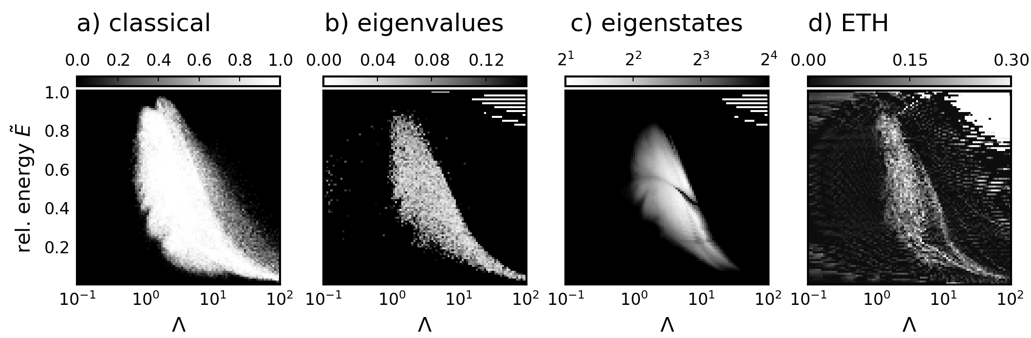
Figure 1: Heatmap of classical chaos indicator a) and quantum chaos indicators b), c) and d). Relative energy 0 corresponds to the minimal (ground state) energy while 1 corresponds to the maximal energy and $\Lambda$ is the onsite interaction strength. The lighter the color the more chaotic. a) Fraction of states with positive largest Lyapunov exponent b) Kullback-Leibler divergence of the distribution of level ratios from the distribution of level ratios of Gaussian orthogonal matrices; capped at 0.15. c) Excess kurtosis of eigenstates; capped at $2^{4}$. d) Exponent of the exponential decay of ETH fluctuations with Hilbert space size of normalized operators, clipped between 0 and 0.3.

We will compare the FTLEs for the classical system to several chaos indicators on the quantum side — level statistics, eigenstate statistics, and the scaling of fluctuations of eigenstate expectation values (EEVs). Figure 1 provides an overview of the results. Here we show chaoticity as a function of interaction parameter $\Lambda$ and relative energy. Chaos is visualized as greyscale heatmaps, where the intensity indicates how chaotic that region is — the lighter the more chaotic.

Figure 1 a) shows chaos of the classical Bose-Hubbard model, while b), c) and d) show chaos measures of the quantum system. In a) we show the fraction of positive FTLEs of the classical model. We consider a FTLE as positive if it is greater than $10^{-4}$, and zero otherwise. In b) we show the deviation of level statistics of the quantum model from Wigner’s GOE distribution measured by the Kullback-Leibler divergence. In c) we show how much eigenstates of the quantum model deviate from Gaussian states via the kurtosis. The kurtosis obtained from the eigenstate coefficients in two different bases are combined — the larger of the two is used at every point of the heatmap. In d) we show the exponent in the size-dependence of the fluctuations of eigenstate expectation values (EEV’s). This is motivated by the scaling of the eigenstate thermalization hypothesis (ETH) and may be described as the size dependence of ETH fluctuations in approaching the classical limit [65]. The data in panels b), c) are for $N=150$ bosons, while the exponents in d) are obtained by fitting EEV fluctuations between $N=90$ and $N=170$. Overall, we have found these quantum results to be broadly independent of $N$.

Figure 1 a) reveals features of the classical phase space, i.e., the phase space of the three-site discrete nonlinear Schrödinger equation. For $\Lambda\lesssim 1$ all Lyapunov exponents are close to 0. For $\Lambda>1$ regions with a non-zero fraction of positive Lyapunov exponents emerge at intermediate energies. At $\Lambda\approx 3$ there are positive largest FTLEs at most energies, except for smallest and largest energies. For $\Lambda>3$ the region of non-zero fractions of positive Lyapunov exponents shrinks and shifts to lower energies, where it survives even for the largest $\Lambda=100$ we investigated. These results highlight the mixed nature of the classical phase space. In particular, zero and non-zero Lyapunov exponents exist at the same energy for the same $\Lambda$. This will be further elaborated in section III and figure 2.

The same shape of the heatmap in figure 1 a) is observed in b) – d) as well. The white bars at the top right of the quantum plots do not show chaotic regions; these are finite size defects (gaps in the spectra which are larger than the energy windows used to compile the heatmaps). The exact measures used in these panels and the subtleties encountered for the quantum cases will be detailed in Sections IV, V and VI, which focus respectively on level statistics, panel b), on eigenstate amplitude statistics, panel c), and on EEV scaling, panel d).

The overall visual agreement between classical chaos regions, panel a), and quantum chaos regions, panels b)–d), is striking. Chaotic energy regions of the classical phase space correspond generally to chaotic regions of the spectrum of the quantum Hamiltonian. Even fine structures in the heatmaps show some agreement. For $1<\Lambda<3$ small bulbs appear at the chaotic-regular boundary in the classical spectrum a), which can be recognized in the level statistics b) as well as in the kurtosis of eigenstates c). We conclude that overall there is a close correspondence of chaotic and non-chaotic regions of the classical model and the quantum model. There are, of course, some discrepancies, also among the various quantum measures, and various artifacts due to the particular measures used. These issues will be discussed in the body of this paper.

In section II we introduce the version of the quantum Bose-Hubbard model we use, and its classical limit. Lyapunov exponents of the classical model are analyzed in section III, where the data of figure 1a) is explained, and other ways of using the FTLEs to demarcate chaotic and non-chaotic regions are explored. In section IV we investigate the eigenvalues of the quantum model leading to the results shown in figure 1b). In section V eigenstates are compared to Gaussian states and the numerical derivation of figure 1c) is explained. In section VI, we describe quantifying chaos using EEV scaling exponents, and explain how figure 1d) is obtained. We end the main text with some discussion in section VII. In the Appendices, we provide an outline of how to calculate Lyapunov exponents, and we also show and briefly discuss Lyapunov exponents for $L=4$ and $L=7$ sites.

II Model and parametrizations

II.1 Quantum model and classical limit

We will investigate Bose-Hubbard systems restricted to open-boundary chains of length $L$, with nearest neighbor hoppings and on-site interactions. The quantum Hamiltonian is

$$H=-\frac{1}{2}\sum_{\langle j,l\rangle}J_{j,l}a_{j}^{\dagger}a_{l}+\frac{U}{2}\sum_{j=1}^{L}n_{j}(n_{j}-1),$$ (1)

where $\langle j,l\rangle$ denotes summation over adjacent sites ($l=j\pm 1$), $a_{j}^{\dagger}$ and $a_{j}$ are the bosonic creation and annihilation operators for the $j$-th site and $n_{j}=a_{j}^{\dagger}a_{j}$ is the corresponding occupation number operator. $J_{j,l}=J_{l,j}$ is the symmetric tunneling coefficient and $U$ is the two-particle on-site interaction strength. We choose $J_{1,2}=1.5$ and $J_{j,l}=1$ for $j,l\geq 2$ to avoid reflection symmetry. The number of bosons $N$ is conserved by the Hamiltonian. We introduce the tuning parameter $\Lambda=UN$. The Hilbert space dimension $D$ of the quantum Hamiltonian is $D=\binom{N+L-1}{L-1}$. For constant $L$, this grows with boson number $N$ as $D\sim N^{L-1}$.

The Bose-Hubbard model has a classical limit for $N\to\infty$ while keeping the number of sites $L$ fixed. This limit can be taken by renormalizing the creation and annihilation operators via $a\to a/\sqrt{N}=\bar{a}$, so $[\bar{a}^{\dagger}_{j},\bar{a}_{j}]=1/N=\hbar_{eff}\to 0$ for $N\to\infty$, where we let $\hbar=1$. The renormalized Hamiltonian is then given by

$$\bar{H}=H/N=-\frac{1}{2}\sum_{\langle j,l\rangle}J_{j,l}\bar{a}_{j}^{\dagger}\bar{a}_{l}+\frac{\Lambda}{2}\sum_{j}\bar{n}_{j}(\bar{n}_{j}-1/N),$$ (2)

where $\bar{n}=\bar{a}^{\dagger}\bar{a}$. The corresponding classical Hamiltonian $\mathcal{H}$ in the large $N$-limit is then obtained by replacing the operators $\bar{a}$, $\bar{a}^{\dagger}$ by complex numbers $\psi$, $\psi^{*}$:

$$\mathcal{H}=-\frac{1}{2}\sum_{\langle j,l\rangle}J_{j,l}\psi_{j}^{*}\psi_{l}+\frac{\Lambda}{2}\sum_{j}|\psi_{j}|^{4}.$$ (3)

Conservation of the total number of particles $N$ in the quantum systems enforces

$$\sum_{j}|\psi_{j}|^{2}=1,$$ (4)

so the phase space of the classical model is restricted to the real hyper-sphere $S^{2L-1}\subset\mathbb{R}^{2L}$.

The dynamics of the classical Bose-Hubbard Hamiltonian are given by Hamilton’s equations of motion

$$i\frac{\partial}{\partial t}\psi_{j}=\frac{\partial\mathcal{H}}{\partial\psi_{j}^{*}}=-\frac{1}{2}\sum_{\langle j,l\rangle}J_{j,l}\psi_{l}+\Lambda|\psi_{j}|^{2}\psi_{j},$$ (5)

which is also known as the discrete nonlinear Schrödinger equation, or the discrete Gross-Pitaevskii equation.

Identifying the complex plane $\mathbb{C}$ with the real plane $\mathbb{R}^{2}$ one can rewrite the $L$ complex equations in Eq. (5) as $2L$ real equations. For computational reasons we chose Cartesian coordinates and let $x=\operatorname{Re}\psi$ and $y=\operatorname{Im}\psi$. Then Hamilton’s equation of motion read

$$\frac{\partial\mathcal{H}}{\partial x_{j}}=-\sum_{\langle j,k\rangle}J_{j,k}x_{k}+2\Lambda\sum_{j}(x_{j}^{2}+y_{j}^{2})x_{j}$$ (6)

and

$$\frac{\partial\mathcal{H}}{\partial y_{j}}=-\sum_{\langle j,k\rangle}J_{j,k}y_{k}+2\Lambda\sum_{j}(x_{j}^{2}+y_{j}^{2})y_{j}.$$ (7)

In the limits $\Lambda\to 0$ and $\Lambda\to\infty$, both the quantum and the classical systems are integrable. If $\Lambda=0$ then Eq. (1) and Eq. (3) reduce to free particle Hamiltonians.

If $\Lambda\to\infty$ then one effectively can neglect $J$, so that Eq. (1) is diagonal in the computational basis of mutual eigenstates of $n_{j}$ and the equations of motion Eq. (5) are decoupled.

In the remainder of the paper we mainly focus on the Bose-Hubbard model on $L=3$ sites, so as to focus on a system with very mixed behavior. Computationally, since the Hilbert space size $D$ grows only quadratically in $N$ for $L=3$, we are able to consider the quantum Hamiltonian far into the classical limit (small $\hbar_{eff}=1/N$) while keeping the Hilbert space size accessible for numerical diagonalization.

II.2 Relative energy and energy intervals

Our classical-quantum comparison is energy-resolved. For each $\Lambda$, we will compare the degree of chaos in individual energy regions of the classical system with the degree of chaos in corresponding energy regions of the quantum system.

Numerically, for each interaction $\Lambda$ the possible energies are divided into 100 evenly spaced energy intervals. We also rescale and shift the energy for each $\Lambda$ to define the relative energy

$$\tilde{E}=\frac{E-E_{\min}}{E_{\max}-E_{\min}}$$ (8)

which takes values in the range $[0,1]$. For the classical system, $E_{\min}$ and $E_{\max}$ are the lowest and highest possible classical energies. For the quantum system, they are respectively the lowest eigenenergy (ground state energy) and the highest eigenenergy. Each energy interval corresponds to an interval of $\tilde{E}$ having width $0.01$. When we refer to the interval at relative energy $\tilde{E}$, we mean the interval $[\tilde{E}-0.01,\tilde{E}]$.

For the classical calculation (figure 1a, section III), Lyapunov exponents are collected for phase space points whose energy is in the desired interval. For the quantum eigenvalue statistics (figure 1b, section IV), the spacing between eigenvalues within the desired interval is analyzed. For quantum measures based on eigenstates (figure 1c and 1d, sections V and VI), all eigenstates whose eigenvalues lie in the interval are considered.

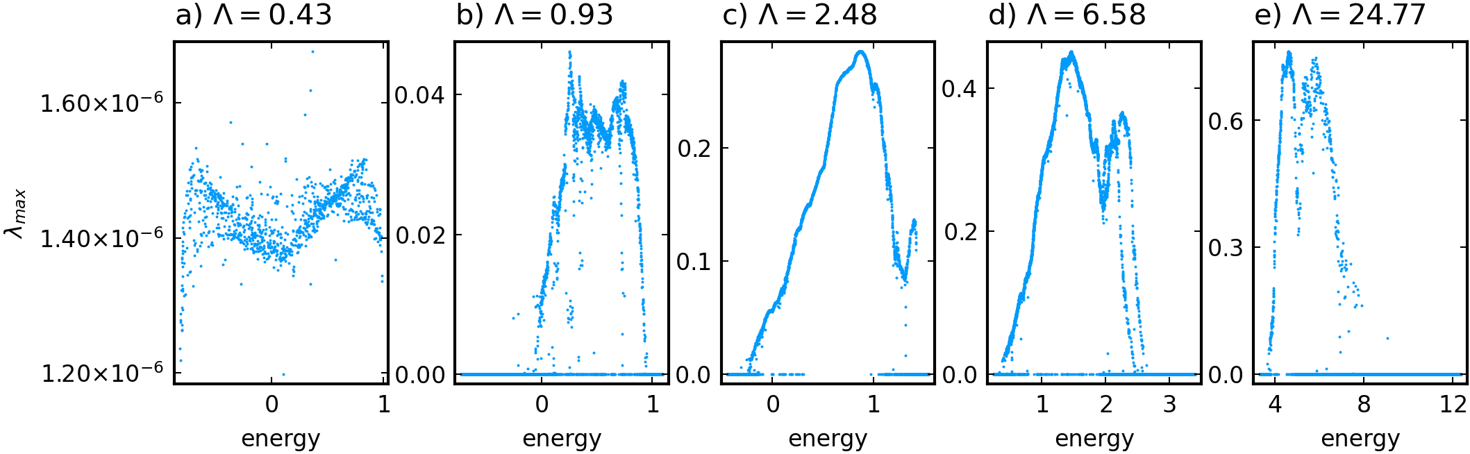
Figure 2: FTLE estimates for largest Lyapunov exponent $\lambda_{\text{max}}$ for the classical limit, Eq. (5). The numerical estimates for $\lambda_{\text{max}}$ are plotted against energy, for several different values of the interaction parameter $\Lambda$.

III Classical Lyapunov exponents

In this section we describe the largest Lyapunov exponents, $\lambda_{\rm max}$, of the classical model, Eq. (5). Some background on Lyapunov exponents and their numerical calculation (calculating FTLE’s) is provided in Appendix B.

In ergodic Hamiltonian systems, $\lambda_{\rm max}$ depends solely on the single conserved quantity, the energy. We will show that the Bose-Hubbard system on three sites is not an ergodic system in this sense — there exist states with the same energy but different largest Lyapunov exponents.

III.1 Preliminaries

For the $L$-site system, because there are $2L$ real equations of motion, we have $2L$ different Lyapunov exponents $\lambda_{\text{max}}=\lambda_{1}\geq\dots\geq\lambda_{2L}$. These exponents are arranged in $L$ pairs of equal magnitude and opposite sign. Two pairs are zero because of the conservation of energy and the conservation of norm, Eq. (4). Thus at most $L-2$ exponents can be positive. For $L=3$, which we will focus on, there is at most one positive Lyapunov exponent. This is $\lambda_{\text{max}}$.

The classical phase space is continuous, so a numerical calculation of the Lyapunov exponents for all states is not possible. One could sample states according to a uniform distribution on the phase space. Due to the conservation of total norm (4), the classical phase space is restricted to the sphere $S^{5}$ in $\mathbb{R}^{6}$. Choosing the $2L$ components of the state from a Gaussian distribution, and then normalizing the resulting state, amounts to sampling uniformly on $S^{5}$. Unfortunately, sampling uniformly on $S^{5}$ can lead to a dearth of samples for small energies and large energies. To sample uniformly in energy we divide the energy spectrum into 100 evenly spaced intervals and sample states uniformly within these energy intervals by the rejection method. We sample states uniformly on $S^{5}$ and reject samples unless the energy of the state lies in the desired energy interval. In this way for each interaction $\Lambda$ we sample up to $10^{4}$ states uniformly distributed in energy.

Obtaining good estimates of Lyapunov exponents is numerically challenging for imperfectly chaotic systems. The system needs to be evolved for long times. The FTLE’s presented in this work are obtained by evolving up to one million time units.

III.2 Numerical observations

In figure 2 we plot FTLE’s of sampled states against the energy of these states, for several interaction parameters $\Lambda$. Only estimates of the largest Lyapunov exponent $\lambda_{\rm max}$ are presented — the other LE’s are either zero or the negative of $\lambda_{\rm max}$.

For $\Lambda=0$, the model is integrable and hence $\lambda_{\text{max}}=0$.

Figure 2a) shows the numerical estimates for $\lambda_{\text{max}}$ for non-zero but still small $\Lambda$ ($\Lambda\approx 0.43$). The numerical estimates for all six Lyapunov exponents have the same order of magnitude, $10^{-6}$. This implies that $\lambda_{\text{max}}$ is either zero or vanishingly small up to some finite value of the interaction.

For larger $\Lambda$, panels b)-e), we find cases of $\lambda_{\text{max}}$ being unambiguously zero, together with cases of the FTLE being smaller than the cutoff $10^{-4}$, which we interpret as $\lambda_{\text{max}}$ being zero. In each of these panels, there are low-energy and high-energy regimes where there are only zero $\lambda_{\text{max}}$, and a central energy regime with nonzero positive $\lambda_{\text{max}}$. For smaller $\Lambda$, the positive-$\lambda_{\text{max}}$ behavior is concentrated at higher energies (there is an extended $\lambda_{\text{max}}=0$ range of low energies), panel b). For large $\Lambda$, the converse is true: $\lambda_{\text{max}}>0$ is seen at lower energies, panel d),e).

In general, when there are nonzero exponents, they coexist with zero exponents at the same energy, i.e., the $\lambda_{\text{max}}$ vs energy function is multi-valued. The only exception is in the intermediate-interaction panel c), $\Lambda\approx 2.48$, for which an energy window with a single nonzero branch is seen. In fact, for any $\Lambda\gtrapprox 1$, there appears always to be some energy window where $\lambda_{\text{max}}$ is multi-valued — we did not see any exceptions.

The coexistence of zero and nonzero $\lambda_{\text{max}}$ is a peculiar manifestation of the mixed nature of the system. This is in contrast to integrable systems (for which $\lambda_{\text{max}}$ is always zero except a measure zero set) and to strongly chaotic or ergodic systems (for which $\lambda_{\text{max}}$ is always positive except a measure zero set). To highlight this contrast, we give examples of systems with stronger chaos, the same Hamiltonian on $L=4$ sites and $L=7$ sites, in the appendix, figure 8.

In an ergodic system the largest Lyapunov exponent is a smooth single valued function of energy. We showed that $\lambda_{\rm max}$ is not a single valued function, but rather often has two branches. One can ask whether each branch is smooth. There are some noisy features in the plots, especially in panels a), b) and e). Presumably, these are finite-time effects, and each branch would resolve into smooth lines if we could integrate up to infinite times. While this conjecture could not be verified conclusively, we observed that integrating up to longer times generally reduces the noisy aspect.

In one case, panel d), $\lambda_{\rm max}$ even appears to have three branches (one zero and two nonzero). We have not seen any indication that this is a finite-time effect, although we cannot rule it out. The data suggests that the mixed nature of the system even allows for three $\lambda_{\rm max}$ values. Apparently, the same fixed-energy region of phase space can consist of a regular (non-chaotic) sub-manifold as well as two different sub-manifolds with different nonzero $\lambda_{\rm max}$!

In figure 1 a) we used as an indicator of chaos the fraction of $\lambda_{\rm max}$ which are nonzero; the same measure has been used in Ref. [67].

III.3 Using the magnitude of Lyapunov exponents

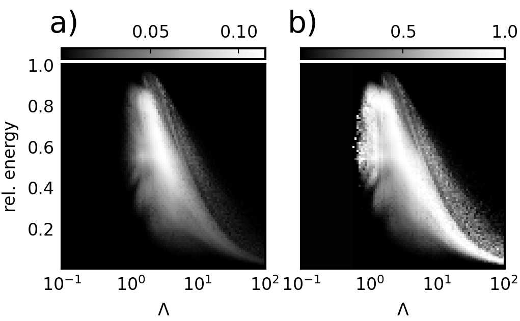
Figure 3: Average largest Lyapunov exponent $\bar{\lambda}_{\rm max}$ per relative energy interval renormalized by a) $\beta_{\Lambda}$ given by Eq. (9) and b) $\gamma_{\Lambda}$ given by Eq. (10).

The procedure of using the fraction of non-zero $\lambda_{\rm max}$’s to characterize chaos neglects the magnitudes of $\lambda_{\rm max}$ altogether. One could also make use of the magnitude as a chaos indicator. This raises the issue of comparing values of $\lambda_{\rm max}$ for different systems (systems with different interactions $\Lambda$). We consider two ways of rescaling the $\lambda_{\rm max}$ values; the resulting heatmaps in figure 3 show reasonable agreement with that in figure 1a).

The magnitude of $\lambda_{\text{max}}$ depends on the timescales of the dynamics of the system. From Eq. (5) one could expect that the dominant timescale will be given by the inverse of the maximum of the Hamiltonian parameters, $J$ and $\Lambda$. We fixed $J_{12}=1.5$ and $J_{23}=1$ throughout the paper so $\max(J,\Lambda)=\max(1.5,\Lambda)$. In figure 3 a) we show the average largest Lyapunov exponent $\overline{\lambda}_{\text{max}}$ per energy interval, rescaled by

$$\beta_{\Lambda}=\max(1.5,\Lambda).$$ (9)

The resulting heatmap in figure 3a), by construction, shows appreciable chaos in the same region as in figure 1a). But figure 3a) shows more detail as it encapsulates the information about the magnitude of $\lambda_{\text{max}}$ as well. We observe the highest intensities in the mid of the spectrum for $1<\Lambda<10$. From there it falls of in all directions. At the top end of figure 3a) we observe a dip in intensity and a sudden increase again, before $\bar{\lambda}_{\rm max}$ becomes zero. These reflect the dips seen in figure 2 c) and d).

Another approach is to rescale all largest Lyapunov exponents in a system with fixed interaction $\Lambda$ by the maximal largest Lyapunov exponent $\lambda_{\text{max}}$ in that specific system. A problem occurs when all largest Lyapunov exponents are close to zero, as for Bose-Hubbard systems with $\Lambda\ll 1$. In these systems there is simply no appreciable positive $\lambda_{\text{max}}$. Therefore we choose the cutoff $10^{-4}$ by which all Lyapunov exponents are minimally divided. The rescaling parameter is

$$\gamma_{\Lambda}=\max(10^{-4},\max_{\psi}\lambda_{\text{max}}(\psi)),$$ (10)

where the maximum runs over all states $\psi$ in the phase space and $\lambda_{\text{max}}(\psi)$ denotes the corresponding largest Lyapunov exponent. A heatmap of the average largest Lyapunov exponent $\bar{\lambda}_{\rm max}$ with this rescaling is shown in figure 3b).

The overall features are the same as in panel 3a). There are some artifacts at the boundary between chaotic and non-chaotic regions, around $\Lambda\approx 0.7$ in panel b), presumably because of numerical uncertainties when $\lambda_{\text{max}}$ is around $10^{-4}$. The intensity of the heatmap does not decrease with $\Lambda$ beyond $\Lambda\approx 10$, unlike panel a) where this decrease is built into the scaling function $\beta_{\Lambda}$.

IV Eigenvalue statistics

In this section we will compare the distribution of spacing ratios of energy levels of the Bose-Hubbard trimer to the level ratio distribution of Gaussian orthogonal random matrices and Poisson level ratios. We will compare the first moment and the whole distribution and describe how we numerically obtain the results leading to figure 1b).

IV.1 Definitions & Background

For ordered energy levels $E_{\alpha}<E_{\alpha+1}$ of a Hamiltonian we denote energy level spacings by $s_{\alpha}=E_{\alpha+1}-E_{\alpha}$. Instead of examining the distribution of $s_{\alpha}$ itself, it has become common to investigate instead the distribution of spacing ratios [68, 69]

$$r_{\alpha}=\frac{s_{\alpha+1}}{s_{\alpha}}\quad\text{and}\quad\tilde{r}_{\alpha}=\min\left(r_{\alpha},\frac{1}{r_{\alpha}}\right).$$ (11)

Studying the ratio distribution bypasses the need to unfold the energy spectrum (to account for the density of states). The quantity $\tilde{r}_{\alpha}$ has the additional advantage that it has bounded support, $\tilde{r}_{\alpha}\in[0,1]$. In the following, when we refer to level spacing ratios, we mean $\tilde{r}_{\alpha}$ (and not $r_{\alpha}$).

The level spacing ratio distribution for matrices in the Gaussian Orthogonal Ensemble (GOE) is given approximately by

$$p_{\rm GOE}(\tilde{r})=\frac{2}{Z_{GOE}}\frac{\tilde{r}+\tilde{r}^{2}}{(1+\tilde{r}+\tilde{r}^{2})^{5/2}},$$ (12)

where the normalization constant is $Z_{GOE}=8/27$. This is the expected spectral behavior of highly chaotic systems. For uncorrelated (Poisson) eigenvalues, the ratio distribution is

$$p_{\rm Poi}(\tilde{r})=\frac{2}{(\tilde{r}+1)^{2}}.$$ (13)

In both cases, the distribution is understood to vanish outside $[0,1]$. GOE spectra have level repulsion, $p_{\rm GOE}(0)=0$, while Poisson spectra do not, $p_{\rm Poi}(0)\neq 0$.

It is usual to compare level spacing distributions over the complete spectrum (sometimes omitting spectral edges) with standard distributions like GOE or Poisson. In this work, we would like to characterize the degree chaos at different energies; hence we compare the distributions obtained from the energy levels within each of the energy intervals described in Subsection II.2. Such energy-resolved comparisons of level statistics have appeared e.g., in [70, 54, 65].

To compare with GOE or Poisson distributions, we use a common measure of the difference between two distributions, namely the Kullback-Leibler (KL) divergence [71]. The KL divergence between an observed distribution $P(z)$ and a reference distribution $Q(z)$ is

$$D_{\mathrm{KL}}(P|Q)=\int_{-\infty}^{\infty}P(z)\log\frac{P(z)}{Q(z)}dz.$$ (14)

This quantity vanishes if $P(z)$ is identical to $Q(z)$. Generally, a larger KL divergence indicates stronger deviation of $P(z)$ from $Q(z)$. In this work, $P(z)$ will be the ratio distributions obtained from the Bose-Hubbard energy levels within each energy interval. We will use either the GOE or the Poisson distribution, Eq. (12) or (13), as the reference $Q(z)$.

IV.2 Numerical Observations — entire distribution and KL divergence

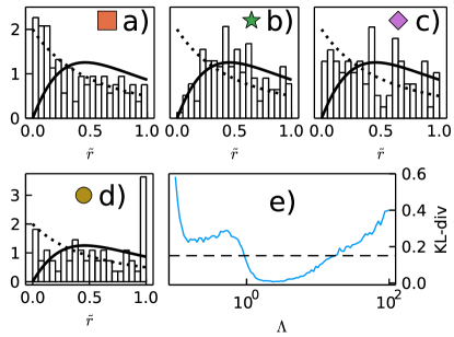
Figure 4: a)–d) Level ratio distributions for combinations of interaction $\Lambda$ and relative energy $\tilde{E}$. a) $\Lambda\approx 0.28$ and $\tilde{E}=0.25$, b) $\Lambda\approx 2.48$ and $\tilde{E}=0.4$, c) $\Lambda\approx 12.33$ and $\tilde{E}=0.65$ and d) $\Lambda\approx 0.28$ and $\tilde{E}=0.13$. Solid and dashed lines are $p_{\text{GOE}}(\tilde{r})$ and $p_{\text{Poi}}(\tilde{r})$, respectively. e) KL divergence of the distribution of the level ratios over the full spectrum from the GOE distribution.

In figures 4 a)-c) we show the observed ratio distributions for three different combinations of relative energy $\tilde{E}$ and interaction parameter $\Lambda$. Since these distributions are estimated from a finite number of energy eigenvalues within the respective energy windows, they are shown as histograms. The data here is extracted from calculations with $N=150$ bosons; the histograms are expected to converge to a smooth distribution in the limit $N\to\infty$.

For visual guidance, the parameters $(\Lambda,\tilde{E})$ corresponding to the panels in figure 4 are marked with respective symbols in figure 5a).

The distribution in panel 4a) is visually seen to be close to the Poisson case. Hence we expect the KL divergence from the Poisson distribution ($D^{\text{Poi}}$) to be small and the KL divergence from the GOE ($D^{\text{GOE}}$) to be large. The situation in panel 4b) is the opposite (close to GOE), while panel 4c) shows an intermediate case. These expectations are borne out by the calculated KL divergences:

a) $$D^{\text{Poi}}\approx 0.05,\quad D^{\text{GOE}}\approx 0.4;$$

b) $$D^{\text{Poi}}\approx 0.22,\quad D^{\text{GOE}}\approx 0.06;$$

c) $$D^{\text{Poi}}\approx 0.16,\quad D^{\text{GOE}}\approx 0.29.$$

In figure 1b), we used $D^{\text{GOE}}$ as a quantifier of chaos and presented its values in the entire $(\Lambda,\tilde{E})$ plane as a heatmap. We capped the values at $0.15$, meaning that values $D^{\text{GOE}}>0.15$ are considered fully non-chaotic and are not distinguished. There is some arbitrariness in the exact choice of this value, but the main results — the overall shape in figure 1b) and its close correspondence with the classical case, figure 1a) — are not strongly affected by the use of a cutoff. In figure 4e), we show $D^{\text{GOE}}$ for the complete energy spectrum as a function of $\Lambda$, to provide a visual sense of the role of the cutoff in separating chaotic from non-chaotic parameter values.

IV.3 Average ratio

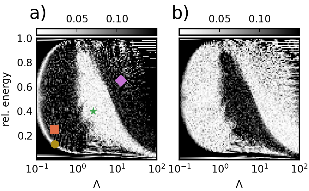
Figure 5: Distance of the mean of the level ratios $\langle\tilde{r}\rangle$ from a) the GOE level ratio mean $\langle\tilde{r}\rangle_{\rm GOE}$ and b) the Poisson level ratio mean $\langle\tilde{r}\rangle_{\rm Poisson}$. The markers in a) indicate the systems shown in figure 4. The square corresponds to figure 4 a), the star to b), the rhombus to c) and the circle to d).

Often only the first moment (mean) of the level ratio distribution is used as a measure of closeness to GOE or Poisson behavior.

The mean of level ratios for the GOE and Poisson cases are $\langle\tilde{r}\rangle_{\rm GOE}\approx 4-2\sqrt{3}\approx 0.53590$ and $\langle\tilde{r}\rangle_{\rm Poi}=2\log 2-1\approx 0.38629$. In cases a), b) and c) above, the means are 0.39, 0.51, and 0.44. i.e., they are respectively close to $\langle\tilde{r}\rangle_{\rm Poi}$, close to $\langle\tilde{r}\rangle_{\rm GOE}$, and intermediate, as expected.

In figure 5 we use the absolute distance from a) $\langle\tilde{r}\rangle_{\rm GOE}$ or from b) $\langle\tilde{r}\rangle_{\rm Poi}$ as possible alternate measures of chaos. Compared to Figure 1 b), we see that the same information is captured — a more chaotic region at intermediate $\Lambda$ and intermediate $\tilde{E}$ is clearly visible in both these cases. Overall, the mean of level ratios is closer to $\langle\tilde{r}\rangle_{\rm GOE}$ inside this region and closer to $\langle\tilde{r}\rangle_{\rm Poi}$ outside. Even the fine structures at the boundary between the two regions, previously seen in the classical case in figure 1a), are visible.

However, there are some artifacts. The most prominent is the arc at the left (small $\Lambda$) region, in figure 5a) The reason is that, at small $\Lambda$, the spectrum shows features specific to the free-boson case, deviating from the Poisson model of completely uncorrelated models. We can see this in figure 4d), which corresponds to a $(\Lambda,\tilde{E})$ combination falling on the arc of panel 5a). The distribution is neither Poisson-like nor GOE-like: it is nonzero for $\tilde{r}\to 0$ and has a pronounced peak at $\tilde{r}\to 1$. Together, these lead to an average $\langle\tilde{r}\rangle\approx 0.52$ which is coincidentally close to $\langle\tilde{r}\rangle_{\rm GOE}$. The deviation from Poisson at very small $\Lambda$ is also seen in panel 5b), in the form of a darker region at the very left of the heatmap.

To summarize: the chaos-regular demarcation in the $(\Lambda,\tilde{E})$ plane can also be visualized using the mean $\langle\tilde{r}\rangle$, modulo some artifacts.

V Eigenstate statistics

In this section, we discuss characterizing chaoticity in the Bose-Hubbard system using the deviation of eigenstate structure from those of GOE matrices. We describe the calculations leading to figure 1c).

The eigenstates of random GOE matrices are uniformly distributed on the $(D-1)$ dimensional unit sphere $S^{D-1}$. For large $D$, a uniform distribution on $S^{D-1}$ is well approximated by a $D$-dimensional Gaussian distribution with independent entries and mean zero and variance $1/D$ [72, 73]. To compare the Bose-Hubbard system with the GOE case, we will compare the coefficients of Bose-Hubbard eigenstates with the Gaussian distribution with mean 0 and variance $1/D$. It has been observed that mid-spectrum eigenstates of chaotic/ergodic many-body systems generally have coefficients with a near-Gaussian distribution [74, 75, 76, 77, 78, 79, 80, 81, 54, 82], in accord with Berry’s conjecture [83]. On the other hand, eigenstates of integrable or many-body-localized systems, as well as eigenstates at the spectral edges of nominally chaotic systems, typically have markedly non-Gaussian distributions [84, 74, 75, 78].

To compare distributions of eigenstate coefficients, we used the excess kurtosis, $\kappa$, of the set of coefficients. The kurtosis is the fourth standardized moment. The excess kurtosis of a distribution is the difference between the kurtosis of that distribution and the kurtosis of a Gaussian distribution, which is 3. Thus, large values of $\kappa$ represent larger deviations from Gaussianity and hence from GOE/chaotic behavior, whereas small values represent more chaotic behavior. When we report values of the kurtosis, we always mean the excess kurtosis $\kappa$, even when the word ‘excess’ is omitted.

The deviation of many-body eigenstates from Gaussianity could also be measured using the KL divergence, as in [75], or using the inverse participation ratio (IPR) or multifractal exponents, as in [84, 85, 77, 78, 86, 54, 55]. We expect these measures to provide very similar overall pictures as the one we present using the kurtosis. In fact, when the mean is negligible (which is true for most eigenstates excepting some at the spectral edges), the kurtosis is proportional to the IPR.

Eigenstate coefficients are defined with respect to a basis. We will investigate eigenstates of the Bose-Hubbard system with respect to three bases:

1. the computational basis, which is given by the mutual eigenstates of the number operators $n_{i}$;

2. the mutual eigenbasis of the hopping operators $a_{i}^{\dagger}a_{j}$, i.e., the eigenbasis of the non-interacting (free) system;

3. the eigenbasis of a perturbed free system with hopping terms $J_{ij}=1$ and small on-site perturbing potentials $\sum_{i}\epsilon_{i}n_{i}$ with values $\epsilon_{1}=-0.01$, $\epsilon_{2}=0.02$ and $\epsilon_{3}=-0.03$ on the three sites.

We name the kurtosis of the coefficients in the three bases as $\kappa_{1}$, $\kappa_{2}$, $\kappa_{3}$ respectively. In Figure 1c), the quantity presented is obtained from a combination of the first and third choices above, namely $\max(\kappa_{1},\kappa_{3})$.

We assume that the distributions underlying the eigenstate components of two eigenstates close in energy are similar. As before, we divide the energy spectrum of each Bose-Hubbard system with interaction strength $\Lambda$ into 100 equally spaced intervals and refer to them by their relative energy $\tilde{E}$. We compute the kurtosis $\kappa$ for every eigenstate and average the calculated kurtosis over each energy interval. If the mean is zero, the averaged kurtosis in an energy interval equals the kurtosis of all components of all eigenstates in that energy interval.

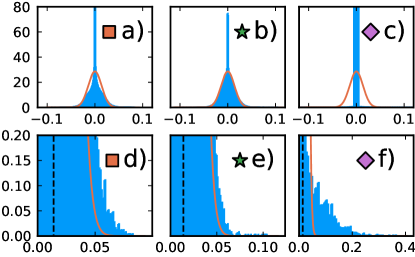
Figure 6: Histograms of eigenstate components of Bose-Hubbard systems with $N=100$ particles, in the computational basis. In a)-c), the interaction and energy intervals, $(\Lambda,\tilde{E})$, are the same as those used in figure 4a)-c). Panels d)-f) are zoomed into the right tails of a)-c). The dashed line indicates the standard deviation. The orange line is a Gaussian density with mean 0 and standard deviation $1/D$. The excess kurtosis is a) $\kappa_{1}\approx 1.6$, b) $\kappa_{1}\approx 0.8$, c) $\kappa_{1}\approx 122$.

In Figure 6a)-c), we show the eigenstate coefficient distributions in the computational ($n_{i}$) basis, for the three $(\Lambda,\tilde{E})$ combinations used previously in Figure 4. (Visual guidance to these three parameter combinations is provided in Figure 5a) and 7a) using corresponding symbols.) The calculated excess kurtosis for these cases are respectively $\kappa_{1}\approx 1.6$, $\kappa_{1}\approx 0.8$ and $\kappa_{1}\approx 122$. The case b) is thus closest to Gaussian, followed by a), while case c) is very far from Gaussian. This is consistent with the visual appearance of the full distributions. It is also consistent with the comparison of the tails of the distibutions against the tails of the Gaussian distribution, as shown in d)-f).

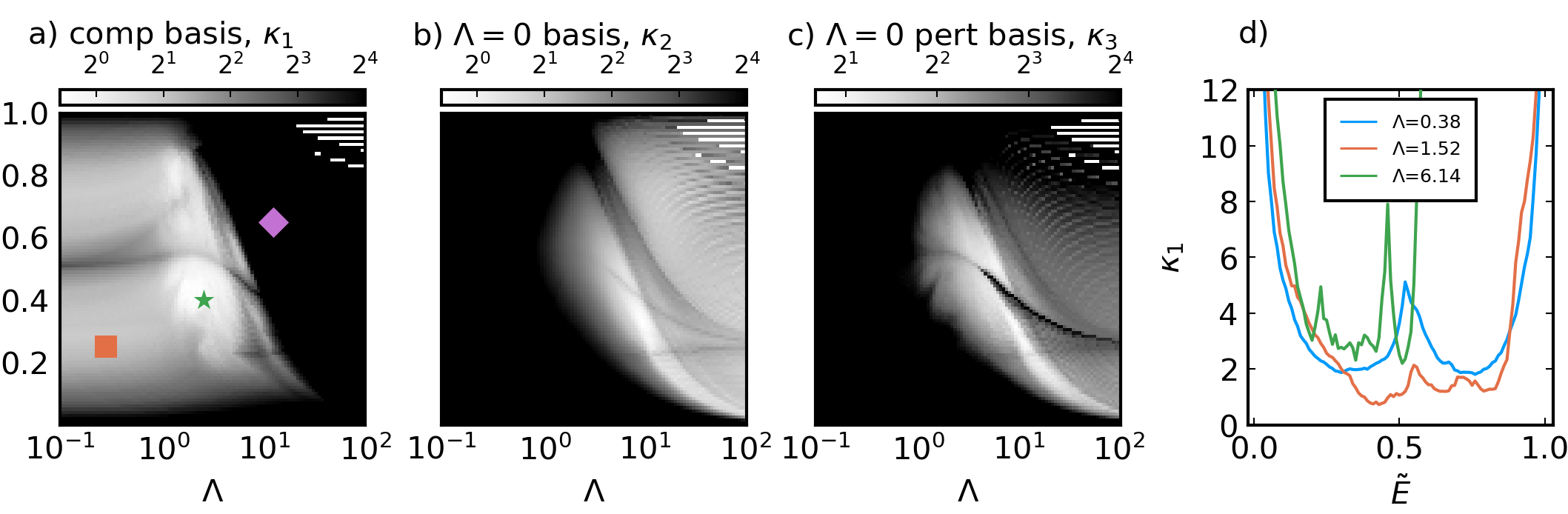
Figure 7: Heatmaps of kurtosis of eigenstate coefficients, for three different bases, listed in the text. The kurtosis is cut off at $2^{4}$ in each case. Markers in a) indicate the $(\Lambda,\tilde{E})$ values for which histograms are shown in Figure 6. The kurtosis heatmap shown in the Introduction, Figure 1b), is a combination of panels a) and c) here — for each $(\Lambda,\tilde{E})$, the larger of the two values is chosen in Figure 1b).

We note in Figure 6b) that the coefficient distribution, although closest to Gaussian, has a large peak near zero. Even in the most chaotic region of the $(\Lambda,\tilde{E})$ plane, the eigenstates depart considerably from the random-matrix case. This is a manifestation of the three-site Bose-Hubbard system being a very mixed system.

In Figure 7a) we show the kurtosis $\kappa_{1}$ for eigenstates in the computational basis as a heatmap in the $(\Lambda,\tilde{E})$ plane. Comparing with previous sections, we see that small $\kappa_{1}$ correlates with non-zero Lyapunov exponents and GOE level statistics, while intermediate and large $\kappa_{1}$ correlates with zero Lyapunov exponents and non-GOE level statistics. The shape of the small-$\kappa_{1}$ region matches the more chaotic region identified previously using classical Lyapunov exponents or using level statistics. Even subtle features from the heatmaps in the previous sections, such as the bulges around $\Lambda\approx 1$ and $\tilde{E}\approx 0.5$ are visible.

For small $\Lambda$, the kurtosis in the computational basis in Figure 7a) shows intermediate rather than large kurtosis, thus failing to fully capture the highly non-chaotic nature of the system in this region. The reason is probably that the small-$\Lambda$ eigenstates are so different from the computational basis states (which are $\Lambda\to\infty$ eigenstates) that they have overlap with a large number of the basis states, leading to a small IPR (hence small kurtosis).

A complementary view is obtained via $\kappa_{2}$ in figure 7b), where $\Lambda=0$ eigenstates have been used as basis. (Because of the large degeneracy at $\Lambda=0$, there is some computational arbitrariness in the choice of this basis.) This basis now has the opposite problem — it fails to show the non-chaotic nature of large-$\Lambda$ region. The problem is partially alleviated by choosing as basis the eigenstates of a non-interacting Hamiltonian with small on-site perturbing potentials; the resulting excess kurtosis $\kappa_{3}$ is shown in figure 7c).

For random-matrix eigenstates, one expects Gaussian behavior with respect to almost any basis. In figure 7, the high-chaos region is marked by low kurtosis in all three basis choices, consistent with the idea of basis-independence. The other regions appear more or less Gaussian-like depending on basis choice. To demarcate the highly chaotic region from less chaotic regions, we can use a combination of kurtosis calculations, taking the larger one from the kurtosis obtained in the first and third basis, i.e., $\max(\kappa_{1},\kappa_{3})$. This is what we did in figure 1b).

VI Scaling of eigenstate expectation values

According to the Eigenstate Thermalization Hypothesis (ETH) [87, 88, 89, 90], the expectation values of physical operators in eigenstates become smooth functions of energy in the thermodynamic limit — the fluctuations of eigenstate expectation values (EEV’s) decreases with system size in a specific manner [91]. Instead of the thermodynamic limit, one could also ask how EEV fluctuations die off in the classical limit $N\to\infty$ [65], which is the limit we are considering in this work. We examine the operator

$$\bar{A}=\frac{a_{2}^{\dagger}a_{1}}{N}.$$

The fluctuations of the EEV’s of this operator, $\sigma(\bar{A})$, scales as a power law,

$$\sigma(\bar{A})\sim D^{-e},$$

with the Hilbert space dimension $D=\binom{N+L-1}{L-1}$. If the eigenstates of the system were fully chaotic, i.e., if the eigenstate coefficients were well-approximated by Gaussian independent variables, one can show that the scaling exponent would be $e=\frac{1}{2}$ [65]. The deviation from $e=\frac{1}{2}$ is thus a measure of departure from chaoticity.

In Figure 1d), we have presented a heatmap of the exponents $e$, determined numerically, for each energy window and interaction parameter. The exponents are determined by fitting the $\sigma(\bar{A})$ vs $D$ data, for system sizes ranging from $N=90$ to $N=170$ in steps of $10$, i.e., $D$ ranging from $\approx 4000$ to $\approx 15000$. As found in Ref. [65], even in the most chaotic regions of the $(\Lambda,\tilde{E})$ plane, the exponent falls well below the ideal value $\frac{1}{2}$. The numerically observed exponent ranges from $0$ in the regular regions to $\approx 0.3$ in the most chaotic regions. The resulting heatmap, Figure 1d), is noisier and less sharp than those obtained from the other measures discussed in previous sections. But the overall demarcation of chaotic and non-chaotic regimes is clearly visible.

VII Context and Discussion

In this article we considered a quantum many-body model that has a classical limit and is well-known to be ‘mixed’, the Bose-Hubbard trimer. We compared the classical Lyapunov exponents of the classical limit against quantum measures of chaos obtained from eigenvalues (statistics of level spacing ratios) and eigenstates (coefficient statistics, fluctuations of expectation values of an operator). Overall, the agreement in the chaos-regular demarcation between the classical case and the various quantum measures is very good.

This reflects the general agreement of chaos measures between quantum systems and their classical limit, when such a limit exists, observed computationally in many different Hamiltonian systems over decades. Perhaps most prominently, single-particle systems in a potential (‘billiards’) have an obvious classical limit — one simply treats the system classically. The literature on quantum-classical correspondence in different billiard systems is vast. Other than billiards, classical and quantum chaos measures have been compared in coupled rotors or coupled tops [9, 10, 92, 19, 93],

bosonic systems [48, 51, 53], the Dicke model and other spin-boson systems [94, 95, 96, 97, 67, 98, 99, 100, 101, 102], the Sherrington-Kirkpatrick model [103], and spin systems [14, 17, 104, 105]. A common theme is that, for spin systems or systems with angular momentum, the large-spin (or large angular momentum) limit is the classical limit, whereas for bosonic systems, the large-boson-number system is the classical limit.

For classical systems, it is common in the literature to demarcate chaotic and non-chaotic regimes using Poincaré sections [9, 12, 13, 14, 14, 94, 95, 100, 101]. We have focused instead on the Lyapunov exponent, and presented it as a multi-branched function of energy. Inspired by Ref. [67], we have used the fraction of Lyapunov exponents which are positive as a chaos measure, and compared it with other ways of exploiting the FTLE results to demarcate highly chaotic and less chaotic behaviors. It is clear that, if the phase space at fixed energy is separated into regular and chaotic regions, then the Lyapunov exponent plotted against energy (with many phase space points sampled in each energy window) will have to be a multi-valued plot. We hope that explicitly presenting and analyzing this multi-valued dependence will contribute to the intuition available on mixed systems.

For quantum systems, we used several measures: (1) the statistics of level spacing ratios based on eigenvalues alone; (2) the coefficients of eigenstates, based on eigenstates expressed in different bases; (3) the scaling of fluctuations of eigenstate expectation values (EEVs), based on eigenstate properties. Level spacing statistics and eigenstate coefficients have been been considered and used as chaos measures for several decades. The EEV fluctuation scaling is based on understanding that has emerged in recent years, motivated by studies of thermalization and ETH.

Of course, there are other interesting measures of quantum chaos that could be considered for comparison. A new candidate is the out-of-time-ordered correlator or OTOC [106, 107, 44, 67] whose behavior (exponential growth) defines a quantum Lyapunov exponent for chaotic systems. For our mixed system, we were unable to unambiguously identify or rule out exponential regimes in the dynamics, for the parameter combinations we attempted. It remains unclear to us whether the OTOC is a useful measure for numerically demarcating more-chaotic parameter regimes from less-chaotic and non-chaotic parameter regimes in mixed systems.

There are some peculiar features in both the eigenvalue and eigenstate statistics, whose origins remain unclear and might be clarified in future studies. In figure 5a, the arc in the small-$\Lambda$ part of the heatmap is due to the level spacing having peculiar statistics, as shown in figure 4d), due to a significant number of successive equal spacings. In the eigenvector statistics, there are some mid-spectrum states that are highly non-Gaussian, even at intermediate $\Lambda$, as seen through the dark nearly horizontal line in figure 7a) at intermediate energies, and the dark curved line in figure 1c), running through the more-chaotic light-colored region at intermediate energies. These might be due to scar-like eigenstates embedded within the more-chaotic eigenstates. Presumably, such peculiar features are less likely to appear in more fully ergodic systems, such as the Bose-Hubbard system with larger number of sites.

Appendix A Lyapunov exponents for more chaotic systems

In figure 8 we present, for comparison, FTLE’s calculated for the 4-site chain and the 7-site chain. The classical Hamiltonian is the same as that presented in Section II.

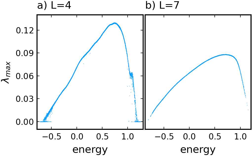
Figure 8: FTLE estimates for the classical largest Lyapunov exponent $\lambda_{\text{max}}$ plotted against energy, for the classical limits of Bose-Hubbard chains with $L=4$ (left) and $L=7$ (right) sites. The interaction parameter is $\Lambda=1.52$. The variational equations were evolved to time $t=10^{6}$.

The systems are increasingly more chaotic with increasing $L$. The arguably most remarkable signature of mixedness in the $L=3$ case was the multi-branched behavior of the Lyapunov exponents, as presented in figure 2 in the main text. For the $L=4$ case, which is more chaotic, some signature of the same phenomenon can be seen at small and large energies, figure 8a). In the $L=7$ case, which is much more chaotic, the phenomenon is absent, figure 8b).

Obtaining good estimates for the Lyapunov exponents is more challenging for mixed systems. Comparing figure 2 and the two panels of figure 8, we see cleaner (less noisy) data for larger $L$, for the same time of propagation, even though there are more variables/equations ($2L$) to be evolved for larger $L$.

Appendix B Numerical calculation of Lyapunov exponents

In this Appendix, we provide an outline of how the largest Lyapunov exponent are estimated numerically [108, 109]. Calculation of the full set of Lyapunov exponents is slightly more involved and so not described here.

We will use the symbol $\psi(t)$ to represent a state or phase space point of the classical system at time $t$. For the Bose-Hubbard chain, $\psi(t)$ is a vector of $L$ complex variables, or $2L$ real variables. The symbol $\psi_{0}$ will be used for the initial state, i.e., $\psi_{0}=\psi(0)$. (In the main text, subscripts to $\psi$ have been used as site indices, but there should be no confusion with our use of the subscript $0$ here.)

Intuitively, the largest Lyapunov exponent $\lambda_{\rm max}$ is given by

$$e^{t\lambda_{\rm max}}\approx\frac{\|\tilde{\psi}(t)-\psi(t)\|}{\|\tilde{\psi}_{0}-\psi_{0}\|},$$ (15)

at large times. Here $\psi(0)=\psi_{0}$ and $\tilde{\psi}(0)=\tilde{\psi}_{0}$ are two initial states which are ‘close’ to each other, and $\psi$ and $\tilde{\psi}$ are time-evolving according to Hamilton’s equations of motion $i\frac{d}{dt}\psi=\frac{\partial\mathcal{H}}{\partial\psi^{*}}$. The largest Lyapunov exponent $\lambda_{\text{max}}$ is independent of the choice of the norm in eq. (15), as long as the phase space is finite-dimensional.

Eq. (15) implies that if the largest Lyapunov exponent $\lambda_{\text{max}}$ is positive the two states $\psi$ and $\psi^{\prime}$ separate exponentially, while a zero largest Lyapunov exponent $\lambda_{\text{max}}=0$ means an at most polynomial spread. For Hamiltonian systems the Lyapunov exponents come in pairs of equal magnitude and opposite sign, so that the largest Lyapunov exponent $\lambda_{\text{max}}$ is at least 0. This is a consequence of Liouville’s theorem.

To calculate the Lyapunov exponent numerically, one might be tempted to choose two initially close states and calculate the right hand side of eq. (15) for large times $t$. Unfortunately, this does not work for bounded systems.

This problem is circumvented by solving the so called variational equations. Denote the time-evolution of the dynamical system corresponding to Hamilton’s equation of motion as

$$\Phi(t,\psi_{0})=\psi(t),\;\text{where }\psi(0)=\psi_{0}.$$ (16)

The dynamical system obeys the semi-group property $\Phi(t+s,x_{0})=\Phi(s,\Phi(t,x_{0}))$ for all times $t$ and $s$. Eq. (15) now reads in terms of $\Phi$ and $\phi_{0}=\psi_{0}-\tilde{\psi}_{0}$ as

$$e^{t\lambda_{\text{max}}}\approx\frac{\|\Phi(t,\psi_{0}+\phi_{0})-\Phi(t,\psi_{0})\|}{\|\phi_{0}\|}.$$ (17)

By linearizing Eq. 17 we obtain the largest Lyapunov exponent as

$$\lambda_{\text{max}}=\lim_{t\to\infty}\frac{1}{t}\log\left\|\partial_{\psi}\Phi(t,\psi)|_{\psi=\psi_{0}}\cdot\frac{\phi_{0}}{\|\phi_{0}\|}\right\|.$$ (18)

Note that $\partial_{\psi}\Phi$ is in general a matrix so the product $\cdot$ denotes the matrix-vector product. The existence of the above limit is ensured by Osedelets theorem [110]. One can show that $\partial_{\psi}\Phi$ evolves in time according to so called variational equations

$$i\frac{d}{dt}\partial_{\psi}\Phi(t,\psi)=\partial_{\psi}\partial_{\psi^{*}}\mathcal{H}(\psi(t))\cdot\partial_{\psi}\Phi(t,\psi),$$ (19)

where $\partial_{\psi}\partial_{\psi^{*}}\mathcal{H}$ denotes the Hessian of the Hamiltonian $\mathcal{H}$ in the variables $\psi$ and $\psi^{*}$ and the initial condition is $\partial_{\psi}\Phi(0,\psi_{0})=\operatorname{Id}$.

In eq. (18) the knowledge of the full matrix $\partial_{\psi}\Phi$ is not required. Only the deviation vector $\phi(t)=\partial_{\psi}\Phi(t,\psi)|_{\psi=\psi_{0}}\phi_{0}/\|\phi_{0}\|$ is needed. The deviation vector evolves according to the variatonal equations (19) as well. This follows from the linearity of $d/dt$.

In principle one could now evolve Hamilton’s equations together with the variational equations to obtain $\phi(t)$ for some large time $t$ and determine $\lambda_{\rm max}$ via eq. (18). However, for positive $\lambda_{\rm max}$ the norm of $\phi(t)$ will blow up exponentially and will quickly be unmanageable by finite precision. This is circumvented by renormalizing $\phi(t)$ and restarting the time evolution, whenever it becomes too large.

References

- Einstein [1917] A. Einstein, Zum Quantensatz von Sommerfeld und Epstein, Verh. Deutsch. Phys. Ges. 19, 82 (1917).
- Schuster and Just [2006] H. Schuster and W. Just, Deterministic Chaos: An Introduction (Wiley, 2006).
- Wigner [1957] E. P. Wigner, Characteristic vectors of bordered matrices with infinite dimensions II (Annals of Mathematics, 1957) pp. 203–207.
- Haake [2010] F. Haake, Quantum Signatures of Chaos, Springer Series in Synergetics (Springer Berlin Heidelberg, 2010).
- Stöckmann [2000] H.-J. Stöckmann, Quantum chaos: an introduction (2000).
- Berry and Tabor [1977] M. Berry and M. Tabor, Level clustering in the regular spectrum, Proceedings of the Royal Society of London. A. Mathematical and Physical Sciences 356, 375 (1977).
- Bohigas et al. [1984a] O. Bohigas, M. J. Giannoni, and C. Schmit, Characterization of chaotic quantum spectra and universality of level fluctuation laws, Phys. Rev. Lett. 52, 1 (1984a).
- Bohigas et al. [1984b] O. Bohigas, M. J. Giannoni, and C. Schmit, Spectral properties of the Laplacian and random matrix theories, Journal de physique. Lettres 45, 1015 (1984b).
- Feingold and Peres [1983] M. Feingold and A. Peres, Regular and chaotic motion of coupled rotators, Physica D: Nonlinear Phenomena 9, 433 (1983).
- Feingold et al. [1984] M. Feingold, N. Moiseyev, and A. Peres, Ergodicity and mixing in quantum theory. ii, Phys. Rev. A 30, 509 (1984).
- Wintgen and Friedrich [1987] D. Wintgen and H. Friedrich, Classical and quantum-mechanical transition between regularity and irregularity in a hamiltonian system, Phys. Rev. A 35, 1464 (1987).
- Bohigas et al. [1993] O. Bohigas, S. Tomsovic, and D. Ullmo, Manifestations of classical phase space structures in quantum mechanics, Physics Reports 223, 43 (1993).
- Dullin et al. [1996] H. R. Dullin, P. H. Richter, and A. Wittek, A two‐parameter study of the extent of chaos in a billiard system, Chaos: An Interdisciplinary Journal of Nonlinear Science 6, 43 (1996).
- Robb and Reichl [1998] D. T. Robb and L. E. Reichl, Chaos in a two-spin system with applied magnetic field, Phys. Rev. E 57, 2458 (1998).
- Ketzmerick et al. [2000] R. Ketzmerick, L. Hufnagel, F. Steinbach, and M. Weiss, New class of eigenstates in generic hamiltonian systems, Phys. Rev. Lett. 85, 1214 (2000).
- Dullin and Bäcker [2001] H. R. Dullin and A. Bäcker, About ergodicity in the family of limaçon billiards, Nonlinearity 14, 1673 (2001).
- Emerson and Ballentine [2001] J. Emerson and L. Ballentine, Characteristics of quantum-classical correspondence for two interacting spins, Phys. Rev. A 63, 052103 (2001).
- Bäcker [2007] A. Bäcker, Random waves and more: Eigenfunctions in chaotic and mixed systems, The European Physical Journal Special Topics 145, 161 (2007).
- Fan et al. [2017] Y. Fan, S. Gnutzmann, and Y. Liang, Quantum chaos for nonstandard symmetry classes in the Feingold-Peres model of coupled tops, Phys. Rev. E 96, 062207 (2017).
- Batistić et al. [2019] B. Batistić, C. Lozej, and M. Robnik, Statistical properties of the localization measure of chaotic eigenstates and the spectral statistics in a mixed-type billiard, Phys. Rev. E 100, 062208 (2019).
- Trombettoni and Smerzi [2001] A. Trombettoni and A. Smerzi, Discrete solitons and breathers with dilute Bose-Einstein condensates, Phys. Rev. Lett. 86, 2353 (2001).
- Smerzi et al. [2002] A. Smerzi, A. Trombettoni, P. G. Kevrekidis, and A. R. Bishop, Dynamical superfluid-insulator transition in a chain of weakly coupled Bose-Einstein condensates, Phys. Rev. Lett. 89, 170402 (2002).
- Smerzi and Trombettoni [2003] A. Smerzi and A. Trombettoni, Nonlinear tight-binding approximation for Bose-Einstein condensates in a lattice, Phys. Rev. A 68, 023613 (2003).
- Kevrekidis [2009] P. Kevrekidis, The Discrete Nonlinear Schrödinger Equation: Mathematical Analysis, Numerical Computations and Physical Perspectives (Springer, 2009).
- Polkovnikov [2003] A. Polkovnikov, Quantum corrections to the dynamics of interacting bosons: Beyond the truncated Wigner approximation, Phys. Rev. A 68, 053604 (2003).
- Mahmud et al. [2005] K. W. Mahmud, H. Perry, and W. P. Reinhardt, Quantum phase-space picture of Bose-Einstein condensates in a double well, Phys. Rev. A 71, 023615 (2005).
- Hiller et al. [2006] M. Hiller, T. Kottos, and T. Geisel, Complexity in parametric Bose-Hubbard Hamiltonians and structural analysis of eigenstates, Phys. Rev. A 73, 061604 (2006).
- Mossmann and Jung [2006] S. Mossmann and C. Jung, Semiclassical approach to Bose-Einstein condensates in a triple well potential, Phys. Rev. A 74, 033601 (2006).
- Graefe and Korsch [2007] E. M. Graefe and H. J. Korsch, Semiclassical quantization of an -particle Bose-Hubbard model, Phys. Rev. A 76, 032116 (2007).
- Trimborn et al. [2009] F. Trimborn, D. Witthaut, and H. J. Korsch, Beyond mean-field dynamics of small Bose-Hubbard systems based on the number-conserving phase-space approach, Phys. Rev. A 79, 013608 (2009).
- Cassidy et al. [2009] A. C. Cassidy, D. Mason, V. Dunjko, and M. Olshanii, Threshold for chaos and thermalization in the one-dimensional mean-field Bose-Hubbard model, Phys. Rev. Lett. 102, 025302 (2009).
- Polkovnikov [2010] A. Polkovnikov, Phase space representation of quantum dynamics, Annals of Physics 325, 1790 (2010).
- Pawłowski et al. [2011] K. Pawłowski, P. Ziń, K. Rzażewski, and M. Trippenbach, Revivals in an attractive Bose-Einstein condensate in a double-well potential and their decoherence, Phys. Rev. A 83, 033606 (2011).
- Simon and Strunz [2012] L. Simon and W. T. Strunz, Analytical results for Josephson dynamics of ultracold bosons, Phys. Rev. A 86, 053625 (2012).
- Simon and Strunz [2014] L. Simon and W. T. Strunz, Time-dependent semiclassics for ultracold bosons, Phys. Rev. A 89, 052112 (2014).
- Veksler and Fishman [2015] H. Veksler and S. Fishman, Semiclassical analysis of Bose-Hubbard dynamics, New Journal of Physics 17, 053030 (2015).
- Engl et al. [2015] T. Engl, J. D. Urbina, and K. Richter, Periodic mean-field solutions and the spectra of discrete bosonic fields: Trace formula for Bose-Hubbard models, Phys. Rev. E 92, 062907 (2015).
- Engl et al. [2016] T. Engl, J. D. Urbina, and K. Richter, The semiclassical propagator in Fock space: dynamical echo and many-body interference, Philosophical Transactions of the Royal Society A: Mathematical, Physical and Engineering Sciences 374, 20150159 (2016).
- Ray et al. [2016a] S. Ray, P. Ostmann, L. Simon, F. Grossmann, and W. T. Strunz, Dynamics of interacting bosons using the Herman-Kluk semiclassical initial value representation, Journal of Physics A: Mathematical and Theoretical 49, 165303 (2016a).
- Dubertrand and Müller [2016] R. Dubertrand and S. Müller, Spectral statistics of chaotic many-body systems, New Journal of Physics 18, 033009 (2016).
- Kidd et al. [2017] R. A. Kidd, M. K. Olsen, and J. F. Corney, Finite-time Lyapunov exponents in chaotic Bose-Hubbard chains, (2017), arXiv:1707.00393 .
- Tomsovic et al. [2018] S. Tomsovic, P. Schlagheck, D. Ullmo, J.-D. Urbina, and K. Richter, Post-Ehrenfest many-body quantum interferences in ultracold atoms far out of equilibrium, Phys. Rev. A 97, 061606 (2018).
- Tomsovic [2018] S. Tomsovic, Complex saddle trajectories for multidimensional quantum wave packet and coherent state propagation: Application to a many-body system, Phys. Rev. E 98, 023301 (2018).
- Rammensee et al. [2018] J. Rammensee, J. D. Urbina, and K. Richter, Many-body quantum interference and the saturation of out-of-time-order correlators, Physical Review Letters 121, 124101 (2018).
- Kidd et al. [2019] R. A. Kidd, M. K. Olsen, and J. F. Corney, Quantum chaos in a Bose-Hubbard dimer with modulated tunneling, Phys. Rev. A 100, 013625 (2019).
- Schlagheck et al. [2019] P. Schlagheck, D. Ullmo, J. D. Urbina, K. Richter, and S. Tomsovic, Enhancement of many-body quantum interference in chaotic bosonic systems: The role of symmetry and dynamics, Phys. Rev. Lett. 123, 215302 (2019).
- Nemoto et al. [2000] K. Nemoto, C. A. Holmes, G. J. Milburn, and W. J. Munro, Quantum dynamics of three coupled atomic Bose-Einstein condensates, Phys. Rev. A 63, 013604 (2000).
- Weiss and Teichmann [2008] C. Weiss and N. Teichmann, Differences between mean-field dynamics and -particle quantum dynamics as a signature of entanglement, Phys. Rev. Lett. 100, 140408 (2008).
- Viscondi and Furuya [2011] T. F. Viscondi and K. Furuya, Dynamics of a Bose-Einstein condensate in a symmetric triple-well trap, Journal of Physics A: Mathematical and Theoretical 44, 175301 (2011).
- Gertjerenken and Weiss [2013] B. Gertjerenken and C. Weiss, Beyond-mean-field behavior of large Bose-Einstein condensates in double-well potentials, Phys. Rev. A 88, 033608 (2013).
- Kolovsky [2016] A. R. Kolovsky, Bose-Hubbard hamiltonian: Quantum chaos approach, International Journal of Modern Physics B 30, 1630009 (2016).
- Heinisch and Holthaus [2016] C. Heinisch and M. Holthaus, Entropy production within a pulsed Bose–Einstein condensate, Zeitschrift für Naturforschung A 71, 875 (2016).
- Rautenberg and Gärttner [2020] M. Rautenberg and M. Gärttner, Classical and quantum chaos in a three-mode bosonic system, Phys. Rev. A 101, 053604 (2020).
- Pausch et al. [2021a] L. Pausch, E. G. Carnio, A. Rodríguez, and A. Buchleitner, Chaos and ergodicity across the energy spectrum of interacting bosons, Phys. Rev. Lett. 126, 150601 (2021a).
- Pausch et al. [2021b] L. Pausch, E. G. Carnio, A. Buchleitner, and A. Rodríguez, Chaos in the Bose-Hubbard model and random two-body Hamiltonians, New Journal of Physics 23, 123036 (2021b).
- Castro et al. [2021] E. R. Castro, J. Chávez-Carlos, I. Roditi, L. F. Santos, and J. G. Hirsch, Quantum-classical correspondence of a system of interacting bosons in a triple-well potential, Quantum 5, 563 (2021), 2105.10515v3 .
- Kolovsky and Buchleitner [2004] A. R. Kolovsky and A. Buchleitner, Quantum chaos in the Bose-Hubbard model, Europhysics Letters (EPL) 68, 632 (2004).
- Kollath et al. [2010] C. Kollath, G. Roux, G. Biroli, and A. M. Läuchli, Statistical properties of the spectrum of the extended Bose-Hubbard model, Journal of Statistical Mechanics: Theory and Experiment 2010, P08011 (2010).
- Hiller et al. [2009] M. Hiller, T. Kottos, and T. Geisel, Wave-packet dynamics in energy space of a chaotic trimeric Bose-Hubbard system, Phys. Rev. A 79, 023621 (2009).
- Arwas et al. [2014] G. Arwas, A. Vardi, and D. Cohen, Triangular Bose-Hubbard trimer as a minimal model for a superfluid circuit, Phys. Rev. A 89, 013601 (2014).
- Vardi [2015] A. Vardi, Chaos, ergodization, and thermalization with few-mode bose-einstein condensates, Rom. Rep. Phys 67, 67 (2015).
- Han and Wu [2016] X. Han and B. Wu, Ehrenfest breakdown of the mean-field dynamics of Bose gases, Phys. Rev. A 93, 023621 (2016).
- Bürkle and Anglin [2019] R. Bürkle and J. R. Anglin, Threshold coupling strength for equilibration between small systems, Phys. Rev. A 99, 063617 (2019).
- Bychek et al. [2020] A. A. Bychek, P. S. Muraev, D. N. Maksimov, E. N. Bulgakov, and A. R. Kolovsky, Chaotic and regular dynamics in the three-site Bose-Hubbard model, AIP Conference Proceedings 2241, 020007 (2020).
- Nakerst and Haque [2021] G. Nakerst and M. Haque, Eigenstate thermalization scaling in approaching the classical limit, Physical Review E 103, 042109 (2021).
- W. et al. [2021] K. W. W., E. R. Castro, A. Foerster, and L. F. Santos, Interacting bosons in a triple well: Preface of many-body quantum chaos, (2021), arXiv:2111.13714 .
- Chávez-Carlos et al. [2019] J. Chávez-Carlos, B. López-del Carpio, M. A. Bastarrachea-Magnani, P. Stránský, S. Lerma-Hernández, L. F. Santos, and J. G. Hirsch, Quantum and classical Lyapunov exponents in atom-field interaction systems, Physical Review Letters 122, 024101 (2019), 1807.10292 .
- Oganesyan and Huse [2007] V. Oganesyan and D. A. Huse, Localization of interacting fermions at high temperature, Phys. Rev. B 75, 155111 (2007).
- Atas et al. [2013] Y. Y. Atas, E. Bogomolny, O. Giraud, and G. Roux, Distribution of the ratio of consecutive level spacings in random matrix ensembles, Phys. Rev. Lett. 110, 084101 (2013).
- Luitz et al. [2015] D. J. Luitz, N. Laflorencie, and F. Alet, Many-body localization edge in the random-field Heisenberg chain, Phys. Rev. B 91, 081103 (2015).
- Kullback and Leibler [1951] S. Kullback and R. A. Leibler, On information and sufficiency, The Annals of Mathematical Statistics 22, 79 (1951).
- Pinelis [2015] I. Pinelis, Exact bounds on the closeness between the Student and standard normal distributions, ESAIM - Probability and Statistics 19, 24 (2015).
- Pinelis and Molzon [2016] I. Pinelis and R. Molzon, Optimal-order bounds on the rate of convergence to normality in the multivariate delta method, Electronic Journal of Statistics 10, 1001 (2016).
- Luitz and Bar Lev [2016] D. J. Luitz and Y. Bar Lev, Anomalous thermalization in ergodic systems, Phys. Rev. Lett. 117, 170404 (2016).
- Beugeling et al. [2018] W. Beugeling, A. Bäcker, R. Moessner, and M. Haque, Statistical properties of eigenstate amplitudes in complex quantum systems, Phys. Rev. E 98, 022204 (2018).
- Khaymovich et al. [2019] I. M. Khaymovich, M. Haque, and P. A. McClarty, Eigenstate thermalization, random matrix theory, and Behemoths, Phys. Rev. Lett. 122, 070601 (2019).
- Bäcker et al. [2019] A. Bäcker, M. Haque, and I. M. Khaymovich, Multifractal dimensions for random matrices, chaotic quantum maps, and many-body systems, Phys. Rev. E 100, 032117 (2019).
- Luitz et al. [2020] D. J. Luitz, I. M. Khaymovich, and Y. B. Lev, Multifractality and its role in anomalous transport in the disordered XXZ spin-chain, SciPost Phys. Core 2, 6 (2020).
- De Tomasi et al. [2021] G. De Tomasi, I. M. Khaymovich, F. Pollmann, and S. Warzel, Rare thermal bubbles at the many-body localization transition from the Fock space point of view, Phys. Rev. B 104, 024202 (2021).
- Srdinšek et al. [2021] M. Srdinšek, T. Prosen, and S. Sotiriadis, Signatures of chaos in nonintegrable models of quantum field theories, Phys. Rev. Lett. 126, 121602 (2021).
- Sugimoto et al. [2021] S. Sugimoto, R. Hamazaki, and M. Ueda, Test of the eigenstate thermalization hypothesis based on local random matrix theory, Phys. Rev. Lett. 126, 120602 (2021).
- Haque et al. [2022] M. Haque, P. A. McClarty, and I. M. Khaymovich, Entanglement of midspectrum eigenstates of chaotic many-body systems: Reasons for deviation from random ensembles, Phys. Rev. E 105, 014109 (2022).
- Berry [1977] M. V. Berry, Regular and irregular semiclassical wavefunctions, Journal of Physics A: Mathematical and General 10, 2083 (1977).
- Luca and Scardicchio [2013] A. D. Luca and A. Scardicchio, Ergodicity breaking in a model showing many-body localization, EPL (Europhysics Letters) 101, 37003 (2013).
- Beugeling et al. [2015] W. Beugeling, A. Andreanov, and M. Haque, Global characteristics of all eigenstates of local many-body hamiltonians: participation ratio and entanglement entropy, Journal of Statistical Mechanics: Theory and Experiment 2015, P02002 (2015).
- De Tomasi and Khaymovich [2020] G. De Tomasi and I. M. Khaymovich, Multifractality meets entanglement: Relation for nonergodic extended states, Phys. Rev. Lett. 124, 200602 (2020).
- Deutsch [1991] J. M. Deutsch, Quantum statistical mechanics in a closed system, Phys. Rev. A 43, 2046 (1991).
- Srednicki [1994] M. Srednicki, Chaos and quantum thermalization, Phys. Rev. E 50, 888 (1994).
- Srednicki [1999] M. Srednicki, The approach to thermal equilibrium in quantized chaotic systems, Journal of Physics A: Mathematical and General 32, 1163 (1999).
- Rigol et al. [2008] M. Rigol, V. Dunjko, and M. Olshanii, Thermalization and its mechanism for generic isolated quantum systems, Nature 452, 854 (2008).
- Beugeling et al. [2014] W. Beugeling, R. Moessner, and M. Haque, Finite-size scaling of eigenstate thermalization, Phys. Rev. E 89, 042112 (2014).
- Ballentine [2004] L. E. Ballentine, Quantum-to-classical limit in a hamiltonian system, Phys. Rev. A 70, 032111 (2004).
- Mondal et al. [2020] D. Mondal, S. Sinha, and S. Sinha, Chaos and quantum scars in a coupled top model, Phys. Rev. E 102, 020101 (2020).
- Bastarrachea-Magnani et al. [2014] M. A. Bastarrachea-Magnani, S. Lerma-Hernández, and J. G. Hirsch, Comparative quantum and semiclassical analysis of atom-field systems. ii. chaos and regularity, Phys. Rev. A 89, 032102 (2014).
- Bastarrachea-Magnani et al. [2015] M. A. Bastarrachea-Magnani, B. L. del Carpio, S. Lerma-Hernández, and J. G. Hirsch, Chaos in the Dicke model: quantum and semiclassical analysis, Physica Scripta 90, 068015 (2015).
- Ray et al. [2016b] S. Ray, A. Ghosh, and S. Sinha, Quantum signature of chaos and thermalization in the kicked Dicke model, Phys. Rev. E 94, 032103 (2016b).
- Bastarrachea-Magnani et al. [2016] M. A. Bastarrachea-Magnani, B. López-del Carpio, J. Chávez-Carlos, S. Lerma-Hernández, and J. G. Hirsch, Delocalization and quantum chaos in atom-field systems, Phys. Rev. E 93, 022215 (2016).
- Lewis-Swan et al. [2019] R. Lewis-Swan, A. Safavi-Naini, J. J. Bollinger, and A. M. Rey, Unifying scrambling, thermalization and entanglement through measurement of fidelity out-of-time-order correlators in the Dicke model, Nature communications 10, 1 (2019).
- Lerose and Pappalardi [2020] A. Lerose and S. Pappalardi, Bridging entanglement dynamics and chaos in semiclassical systems, Phys. Rev. A 102, 032404 (2020).
- Wang and Robnik [2020] Q. Wang and M. Robnik, Statistical properties of the localization measure of chaotic eigenstates in the Dicke model, Phys. Rev. E 102, 032212 (2020).
- Villaseñor et al. [2020] D. Villaseñor, S. Pilatowsky-Cameo, M. A. Bastarrachea-Magnani, S. Lerma-Hernández, L. F. Santos, and J. G. Hirsch, Quantum vs classical dynamics in a spin-boson system: manifestations of spectral correlations and scarring, New Journal of Physics 22, 063036 (2020).
- Pilatowsky-Cameo et al. [2021] S. Pilatowsky-Cameo, D. Villaseñor, M. A. Bastarrachea-Magnani, S. Lerma-Hernández, L. F. Santos, and J. G. Hirsch, Quantum scarring in a spin-boson system: fundamental families of periodic orbits, New Journal of Physics 23, 033045 (2021).
- Pappalardi et al. [2020] S. Pappalardi, A. Polkovnikov, and A. Silva, Quantum echo dynamics in the Sherrington-Kirkpatrick model, SciPost Phys. 9, 21 (2020).
- Pappalardi et al. [2018] S. Pappalardi, A. Russomanno, B. Žunkovič, F. Iemini, A. Silva, and R. Fazio, Scrambling and entanglement spreading in long-range spin chains, Phys. Rev. B 98, 134303 (2018).
- Ray et al. [2019] S. Ray, S. Sinha, and D. Sen, Dynamics of quasiperiodically driven spin systems, Phys. Rev. E 100, 052129 (2019).
- Maldacena et al. [2016] J. Maldacena, S. H. Shenker, and D. Stanford, A bound on chaos, Journal of High Energy Physics 2016, 106 (2016).
- Stanford [2016] D. Stanford, Many-body chaos at weak coupling, Journal of High Energy Physics 2016, 9 (2016).
- Benettin et al. [1980a] G. Benettin, L. Galgani, A. Giorgilli, and J.-M. Strelcyn, Lyapunov characteristic exponents for smooth dynamical systems and for Hamiltonian systems; a method for computing all of them. Part 1: Theory, Meccanica 15, 9 (1980a).
- Benettin et al. [1980b] G. Benettin, L. Galgani, A. Giorgilli, and J. Strelcyn, Lyapunov characteristic exponents for smooth dynamical systems and for Hamiltonian systems; a method for computing all of them. Part 2: Numerical application, Meccanica 15, 21 (1980b).
- Oseledets [1968] V. I. Oseledets, A multiplicative ergodic theorem. Characteristic Ljapunov, exponents of dynamical systems, Trudy Moskovskogo Matematicheskogo Obshchestva 19, 179 (1968).