Convergence properties of an Objective-Function-Free
Optimization regularization algorithm, including
an $\mathcal{O}(\epsilon^{-3/2})$ complexity bound

Abstract

An adaptive regularization algorithm for unconstrained nonconvex optimization is presented in which the objective function is never evaluated, but only derivatives are used. This algorithm belongs to the class of adaptive regularization methods, for which optimal worst-case complexity results are known for the standard framework where the objective function is evaluated. It is shown in this paper that these excellent complexity bounds are also valid for the new algorithm, despite the fact that significantly less information is used. In particular, it is shown that, if derivatives of degree one to $p$ are used, the algorithm will find an $\epsilon_{1}$-approximate first-order minimizer in at most ${\cal O}(\epsilon_{1}^{-(p+1)/p})$ iterations, and an $(\epsilon_{1},\epsilon_{2})$-approximate second-order minimizer in at most ${\cal O}(\max[\epsilon_{1}^{-(p+1)/p},\epsilon_{2}^{-(p+1)/(p-1)}])$ iterations. As a special case, the new algorithm using first and second derivatives, when applied to functions with Lipschitz continuous Hessian, will find an iterate $x_{k}$ at which the gradient’s norm is less than $\epsilon_{1}$ in at most ${\cal O}(\epsilon_{1}^{-3/2})$ iterations.

Keywords: nonlinear optimization, adaptive regularization methods, evaluation complexity,
objective-function-free optimization (OFFO).

1 Introduction

This paper is about the (complexity-wise) fastest known optimization method which does not evaluate the objective function. Such methods, coined OFFO for Objective-Function-Free Optimization, have recently been very popular in the context of noisy problems, in particular in deep learning applications (see [26, 18, 32, 31] among many others), where they have shown remarkable insensitivity to the noise level. This is a first motivation to consider them, and it is our point of view that their deterministic (noiseless) counterparts are good stepping stones to understand their behaviour. Another motivation is the observation that other more standard methods (using objective function evaluations) have been proposed in the noisy case, but these typically require the noise on the function values to be tightly controlled at a level lower than that allowed for derivatives [12, 13, 6, 15, 4, 3, 2, 1]

The convergence anaysis of OFFO algorithms is not a new subject, and has been considered for instance in [16, 31, 22, 21, 19, 32]. However, as far as the authors are aware, the existing theory focuses on the case where only gradients are used (with the exception of [25]) and establish a worst-case iteration complexity of, at best, ${\cal O}(\epsilon^{-2})$ for finding an $\epsilon$-approximate first-order stationary point [27]. It is already remarkable that this bound is, in order and for the same goal, identical to that of standard methods using function values. But methods using second-derivatives have proved to be globally more efficient in this latter context, and the (complexity-wise) fastest such method is known to have an ${\cal O}(\epsilon^{-3/2})$ complexity bound [28, 14, 30, 8, 5, 11]. Moreover, this better bound was shown to be sharp and optimal among a large class of optimization algorithms using second-derivatives for the noiseless case [9]. Is such an improvement in complexity also possible for (noiseless) OFFO algorithms? We answer this question positively in what follows.

The theory developed here combines elements of standard adaptive regularization methods such as AR$p$ [5] and of the OFFO approaches of [32] and [19]. We exhibit an OFFO regularization method whose iteration complexity is identical to that obtained when objective function values are used. In particular, we consider convergence to approximate first-order and second-order critical points, and provide sharp complexity bounds depending on the degree of derivatives used.

The paper is organized as follows. After introducing the new algorithm in Section 2, we present and discuss a first-order worst-case complexity analysis in Section 3, while convergence to approximate second-order minimizers is considered in Section 4. Some numerical expirements showing the impact of noise are then presented in Section 5. Conclusions and perspectives are outlined in Section 6.

2 An OFFO adaptive regularization algorithm

We now consider the problem of finding approximate minimizers of the unconstrained nonconvex optimization problem

$$\min_{x\in\hbox{I\hskip-2.0ptR}^{n}}f(x),$$ (2.1)

where $f$ is a sufficiently smooth function from $\hbox{I\hskip-2.0ptR}^{n}$ into IR. As motivated in the introduction, our aim is to design an algorithm in which the objective function value is never computed. Our approach is based on regularization methods. In such methods, a model of the objective function is build by “regularizing” a truncated Taylor expansion of degree $p\geq 1$. We now detail the assumption on the problems that ensure this approach makes sense.

AS.1 $f$ is $p$ times continuously differentiable in $\hbox{I\hskip-2.0ptR}^{n}$.

AS.2 There exists a constant $f_{\rm low}$ such that $f(x)\geq f_{\rm low}$ for all $x\in\hbox{I\hskip-2.0ptR}^{n}$.

AS.3 The $p$th derivative of $f$ is globally Lipshitz continuous, that is, there exist a non-negative constant $L_{p}$ such that

$$\|\nabla_{x}^{p}f(x)-\nabla_{x}^{p}f(y)\|\leq L_{p}\|x-y\|\,\text{ for all }x,y\in\hbox{I\hskip-2.0ptR}^{n},$$ (2.2)

where $\|.\|$ denotes the Euclidean norm in $\hbox{I\hskip-2.0ptR}^{n}$.

AS.4 If $p>1$, there exists a constant $\kappa_{\mbox{\tiny high}}\leq 0$ such that

$$\min_{\|d\|\leq 1}\nabla_{x}^{i}f(x)[d]^{i}\geq\kappa_{\mbox{\tiny high}}\;\;\mbox{for all}\;\;x\in\hbox{I\hskip-2.0ptR}^{n}\;\;\mbox{and}\;\;i\in\{2,\ldots,p\},$$ (2.3)

where $\nabla_{x}^{i}f(x)$ is the $i$th derivative tensor of $f$ computed at $x$, and where $T[d]^{i}$ denotes the $i$-dimensional tensor $T$ applied on $i$ copies of the vector $d$. (For notational convenience, we set $\kappa_{\mbox{\tiny high}}=0$ if $p=1$.)

We note that AS.4 is weaker than assuming uniform boundedness of the derivative tensors of degree two and above (there is no upper bound on the value of $\nabla_{x}^{i}f(x)[d]^{i}$), or, equivalently, Lipschitz continuity of derivatives of degree one to $p-1$.

2.1 The OFFAR$p$ algorithm

Adaptive regularization methods are iterative schemes which compute a step from an iterate $x_{k}$ to the next by approximately minimizing a $p$th degree regularized model $m_{k}(s)$ of $f(x_{k}+s)$ of the form

$$m_{k}(s)\stackrel{{\scriptstyle\rm def}}{{=}}T_{f,p}(x_{k},s)+\frac{\sigma_{k}}{(p+1)!}\|s\|^{p+1},$$ (2.4)

where $T_{f,p}(x,s)$ is the $p$th order Taylor expansion of functional $f$ at $x$ truncated at order $p$, that is,

$$T_{f,p}(x,s)\stackrel{{\scriptstyle\rm def}}{{=}}f(x)+\sum_{i=1}^{p}\frac{1}{i!}\nabla_{x}^{i}f(x)[s]^{i}.$$ (2.5)

In (2.4), the $p$th order Taylor series is “regularized” by adding the term $\frac{\sigma_{k}}{(p+1)!}\|s\|^{p+1}$, where $\sigma_{k}$ is known as the “regularization parameter”. This term guarantees that $m_{k}(s)$ is bounded below and thus makes the procedure of finding a step $s_{k}$ by (approximately) minimizing $m_{k}(s)$ well-defined. Our proposed algorithm follows the outline line of existing AR$p$ regularization methods [8, 5, 11], with the significant difference that the objective function $f(x_{k})$ is never computed, and therefore that the ratio of achieved to predicted reduction (a standard feature for these methods) cannot be used to accept or reject a potential new iterate and to update the regularization parameter. Instead, such potential iterates are always accepted and the regularization parameter is updated in a manner independent of this ratio. We now state the resulting OFFAR$p$ algorithm in detail 2.1.

Algorithm 2.1: OFFO adaptive regularization of degree $p$ (OFFAR$p$)
Step 0: Initialization: An initial point $x_{0}\in\hbox{I\hskip-2.0ptR}^{n}$, a regularization parameter $\nu_{0}>0$ and a requested final gradient accuracy $\epsilon_{1}\in(0,1]$ are given, as well as the parameters $$\theta_{1}>1\;\;\mbox{ and }\;\;\vartheta\in(0,1].$$ (2.6) Set $k=0$. Step 1: Check for termination: Evaluate $g_{k}=\nabla_{x}^{1}f(x_{k})$. Terminate with $x_{\epsilon}=x_{k}$ if $$\|g_{k}\|\leq\epsilon_{1}.$$ (2.7) Else, evaluate $\{\nabla_{x}^{i}f(x_{k})\}_{i=2}^{p}$. Step 2: Step calculation: If $k>0$, set $$\mu_{1,k}=\frac{p!\|g_{k}\|}{\|s_{k-1}\|^{p}}-\theta_{1}\sigma_{k-1}$$ (2.8) and select $$\sigma_{k}\in\left[\vartheta\nu_{k},\max\left(\nu_{k},\mu_{1,k}\right)\right].$$ (2.9) Otherwise (i.e. if $k=0$), set $\sigma_{0}=\mu_{0}=\nu_{0}$.
Then compute a step $s_{k}$ which sufficiently reduces the model $m_{k}$ defined in (2.4) in the sense that $$m_{k}(s_{k})-m_{k}(0)<0$$ (2.10) and $$\|\nabla_{s}^{1}T_{f,p}(x_{k},s_{k})\|\leq\theta_{1}\frac{\sigma_{k}}{p!}\|s_{k}\|^{p}.$$ (2.11) Step 3: Updates. Set $$x_{k+1}=x_{k}+s_{k}$$ (2.12) and $$\nu_{k+1}=\nu_{k}+\nu_{k}\|s_{k}\|^{p+1}.$$ (2.13) Increment $k$ by one and go to Step 1.

The test (2.11) follows [24] and extends the more usual condition where the step $s_{k}$ is chosen to ensure that

$$\|\nabla_{s}^{1}m_{k}(s_{k})\|\leq\theta_{1}\|s_{k}\|^{p}.$$

It is indeed easy to verify that (2.11) holds at a local minimizer of $m_{k}$ with $\theta_{1}\geq 1$ (see [24] for details). The motivation for the introduction of $\mu_{1,k}$ in (2.8) and (2.9) will become clearer after Lemma 3.4.

3 Evaluation complexity for the OFFAR$p$ algorithm

Before discussing our analysis of evaluation complexity, we first restate some classical lemmas for AR$p$ algorithms, starting with Lipschitz error bounds.

Lemma 3.1

Suppose that AS.1 and AS.3 hold. Then $$|f(x_{k+1})-T_{f,p}(x_{k},s_{k})|\leq\frac{L_{p}}{(p+1)!}\|s_{k}\|^{p+1},$$ (3.1) and $$\|g_{k+1}-\nabla_{s}^{1}T_{f,p}(x_{k},s_{k})\|\leq\frac{L_{p}}{p!}\|s_{k}\|^{p}.$$ (3.2)

• Proof.   This is a standard result (see [10, Lemma 2.1] for instance). $\Box$

We start by stating a simple lower bound on the Taylor series’ decrease.

Lemma 3.2

$$\Delta T_{f,p}(x_{k},s_{k})\stackrel{{\scriptstyle\rm def}}{{=}}T_{f,p}(x_{k},0)-T_{f,p}(x_{k},s_{k})\geq\frac{\sigma_{k}}{(p+1)!}\|s_{k}\|^{p+1}.$$ (3.3)

• Proof.   The bound directly results from (2.10) and (2.4). $\Box$

This and AS.2 allow us to establish a lower bound on the decrease in the objective function (although it is never computed).

Lemma 3.3

Suppose that AS.1 and AS.3 hold and that $\sigma_{k}\geq 2L_{p}$. Then $$f(x_{k})-f(x_{k+1})\geq\frac{\sigma_{k}}{2(p+1)!}\|s_{k}\|^{p+1}.$$ (3.4)

• Proof.    From (3.1) and (3.3), we obtain that

  $$f(x_{k})-f(x_{k+1})\geq\frac{\sigma_{k}-L_{p}}{(p+1)!}\|s_{k}\|^{p+1}$$

  and (3.4) immediately follows from our assumption on $\sigma_{k}$. $\Box$

The next lemma provides a useful lower bound on the step length, in the spirit of [5, Lemma 2.3] or [24].

Lemma 3.4

Suppose that AS.1 and AS.3 hold. Then, for all $k\geq 0$, $$\|s_{k}\|^{p}>\frac{p!}{L_{p}+\theta_{1}\sigma_{k}}\|g(x_{k+1})\|,$$ (3.5) $$\mu_{1,k}\leq\max[\nu_{0},L_{p}]$$ (3.6) and $$\sigma_{k}\leq L_{p}+\nu_{k}.$$ (3.7)

• Proof.    Successively using the triangle inequality, condition (2.11) and (3.2), we deduce that

  $$\|{g(x_{k+1})}\|\leq\|g(x_{k+1})-\nabla_{s}^{1}T_{f,p}(x_{k},s_{k})\|+\|\nabla_{s}^{1}T_{f,p}(x_{k},s_{k})\|\leq\frac{\displaystyle 1}{\displaystyle p!}L_{p}\|s_{k}\|^{p}+\theta_{1}\frac{\sigma_{k}}{p!}\|s_{k}\|^{p}.$$

  The inequality (3.5) follows by rearranging the terms. Combining this inequality with (2.8) and the identity $\mu_{0}=\nu_{0}$ then gives (3.6), from which (3.7) directly follows using (2.9). $\Box$

Observe that (3.6) motivates our choice in (2.9) to allow the regularization parameter to be of size $\mu_{1,k}$.

Inspired by [19, Lemma 7], we now establish an upper bound on the number of iterations needed to enter the algorithm’s phase where Lemma 3.3 applies and thus all iterations produce a decrease in the objective function.

Lemma 3.5

Suppose that AS.1 and AS.3 hold, and that the OFFAR$p$ algorithm does not terminate before or at iteration of index $$k\geq k_{*}\stackrel{{\scriptstyle\rm def}}{{=}}\left\lceil\left(\frac{2L_{p}}{\epsilon_{1}\vartheta p!}\left((1+\theta_{1})\frac{L_{p}}{\sigma_{0}}+\theta_{1}\right)\right)^{\scriptstyle\frac{p+1}{p}}\right\rceil.$$ (3.8) Then, $$\nu_{k}\geq\frac{2L_{p}}{\vartheta}$$ (3.9) which implies that $$\sigma_{k}\geq 2L_{p}.$$ (3.10)

• Proof.    Note that (3.10) is a direct consequence of (2.9) if (3.9) is true. Suppose the opposite and that for some $k\geq k_{*}$, $\nu_{k}<\frac{2L_{p}}{\vartheta}$. Since $\nu_{k}$ is a non-decreasing sequence, we have that $\nu_{j}<\frac{2L_{p}}{\vartheta}$ for $j\in\{0,\ldots,k\}$. Successively using the form of the $\nu_{k}$ update rule (2.13), (3.5), (3.7) and the fact that, if the algorithm has reached iteration $k_{*}$, it must be that (2.7) has failed for all iterations of index at most $k_{*}$, we derive that

  $$\nu_{k} >\sum_{j=0}^{k-1}\nu_{j}\|s_{j}\|^{p+1}\geq\sum_{j=0}^{k-1}\nu_{j}\left(\frac{p!\|g(x_{j+1})\|}{L_{p}+\theta_{1}\sigma_{j}}\right)^{{\scriptstyle\frac{p+1}{p}}}\geq\sum_{j=0}^{k-1}\nu_{j}\left(\frac{p!\|g(x_{j+1})\|}{L_{p}+\theta_{1}(L_{p}+\nu_{j})}\right)^{{\scriptstyle\frac{p+1}{p}}}$$

  $$=\sum_{j=0}^{k-1}\nu_{j}^{-{\scriptstyle\frac{1}{p}}}\left(\frac{p!\|g(x_{j+1})\|}{(1+\theta_{1})\frac{L_{p}}{\nu_{j}}+\theta_{1}}\right)^{{\scriptstyle\frac{p+1}{p}}}>\sum_{j=0}^{k-1}\nu_{j}^{-{\scriptstyle\frac{1}{p}}}\left(\frac{p!\|g(x_{j+1})\|}{(1+\theta_{1})\frac{L_{p}}{\sigma_{0}}+\theta_{1}}\right)^{{\scriptstyle\frac{p+1}{p}}}$$

  $$>\frac{\displaystyle k_{*}\,\vartheta^{\scriptstyle\frac{1}{p}}(p!\epsilon_{1})^{{\scriptstyle\frac{p+1}{p}}}}{\displaystyle(2L_{p})^{\scriptstyle\frac{1}{p}}\left((1+\theta_{1})\frac{L_{p}}{\sigma_{0}}+\theta_{1}\right)^{\scriptstyle\frac{p+1}{p}}}.$$

  Substituting the definition of $k_{*}$ in the last inequality, we obtain that

  $$\frac{2L_{p}}{\vartheta}<\nu_{k_{*}}<\frac{2L_{p}}{\vartheta},$$

  which is impossible. Hence no index $k\geq k_{*}$ exists such that $\nu_{k}<\frac{2L_{p}}{\vartheta}$ and (3.9) and (3.10) hold. $\Box$

Observe that (3.8) depends on the ratio $\frac{L_{p}}{\sigma_{0}}$ which is the fraction by which $\sigma_{0}$ underestimates the Lipschitz constant. This ratio will percolate in the rest of our analysis. We now define

$$k_{1}=\min\left\{k\geq 1\mid\nu_{k}\geq\frac{2L_{p}}{\vartheta}\right\},$$ (3.11)

the first iterate such that significant objective function decrease is guaranteed. The next series of Lemmas provide bounds on $f(x_{k_{1}})$ and $\sigma_{k_{1}}$, which in turn will allow establishing an upper bound on the regularization parameter. We start by proving an upper bound on $s_{k}$ generalizing those proposed in [7, 24] to the case where $p$ is arbitrary.

Lemma 3.6

Suppose that AS.1 and AS.4 hold. At each iteration $k$, we have that $$\|s_{k}\|\leq 2\eta+2\left(\frac{(p+1)!\|g_{k}\|}{\sigma_{k}}\right)^{\scriptstyle\frac{1}{p}},$$ (3.12) where $$\eta=\sum_{i=2}^{p}\left[\frac{\max[0,-\kappa_{\mbox{\tiny high}}](p+1)!}{i!\,\vartheta\nu_{0}}\right]^{\scriptstyle\frac{1}{p-i+1}}.$$ (3.13)

• Proof.   If $p=1$, we obtain from (2.10) and the Cauchy-Schwarz inequality that

  $${\scriptstyle\frac{1}{2}}\sigma_{k}\|s_{k}\|^{2}<-g_{k}^{T}s_{k}\leq\|g_{k}\|\,\|s_{k}\|$$

  and (3.12) holds with $\eta=0$. Suppose now that $p>1$. Again (2.10) gives that

  $$\frac{\sigma_{k}}{(p+1)!}\|s_{k}\|^{p+1}\leq-g_{k}^{T}s_{k}-\sum_{i=2}^{p}\frac{1}{i!}\nabla_{x}^{i}f(x_{k})[s_{k}]^{i}\leq\|g_{k}\|\|s_{k}\|+\sum_{i=2}^{p}\frac{\max[0,-\kappa_{\mbox{\tiny high}}]}{i!}\|s_{k}\|^{i}.$$

  Applying now the Lagrange bound for polynomial roots [33, Lecture VI, Lemma 5] with $x=\|s_{k}\|$, $n=p+1$, $a_{0}=0$, $a_{1}=\|g_{k}\|$, $a_{i}=\max[0,-\kappa_{\mbox{\tiny high}}]/i!$ $i\in\{2,\ldots,p\}$ and $a_{p+1}=\sigma_{k}/(p+1)!$, we know from (2.10) that the equation $\sum_{i=0}^{n}a_{i}x^{i}=0$ admits at least one strictly positive root, and we may thus derive that

  $$\|s_{k}\| \leq 2\left(\frac{(p+1)!\|g_{k}\|}{\sigma_{k}}\right)^{\scriptstyle\frac{1}{p}}+2\sum_{i=2}^{p}\left[\frac{\max[0,-\kappa_{\mbox{\tiny high}}](p+1)!}{i!\,\sigma_{k}}\right]^{\scriptstyle\frac{1}{p-i+1}}$$

  $$\leq 2\left(\frac{(p+1)!\|g_{k}\|}{\sigma_{k}}\right)^{\scriptstyle\frac{1}{p}}+2\sum_{i=2}^{p}\left[\frac{\max[0,-\kappa_{\mbox{\tiny high}}](p+1)!}{i!\,\vartheta\nu_{k}}\right]^{\scriptstyle\frac{1}{p-i+1}}$$

  $$\leq 2\left(\frac{(p+1)!\|g_{k}\|}{\sigma_{k}}\right)^{\scriptstyle\frac{1}{p}}+2\sum_{i=2}^{p}\left[\frac{\max[0,-\kappa_{\mbox{\tiny high}}](p+1)!}{i!\,\vartheta\nu_{0}}\right]^{\scriptstyle\frac{1}{p-i+1}},$$

  and (3.12) holds with (3.13). $\Box$

Our next step is to prove that $\nu_{k_{1}}$ is bounded by constants only depending on the problem and the fixed algorithmic parameters.

Lemma 3.7

Suppose that AS.1, AS.3 and AS.4 hold. Let $k_{1}$ be defined by (3.11). We have that, $$\nu_{k_{1}}\leq\nu_{\max}=\max\left[\sigma_{0}+\sigma_{0}\left(2\eta+2\left(\frac{(p+1)!\|g_{0}\|}{\sigma_{0}}\right)^{\scriptstyle\frac{1}{p}}\right)^{p+1},\,\frac{2\kappa_{1}L_{p}}{\vartheta}\right]$$ (3.14) where $\eta$ is defined in (3.13) and $$\kappa_{1}\stackrel{{\scriptstyle\rm def}}{{=}}1+2^{2p+1}\eta^{p+1}+2^{2p+1}\left[\frac{p+1}{\vartheta}\left((1+\theta_{1})\frac{L_{p}}{\sigma_{0}}+\theta_{1}\right)\right]^{\scriptstyle\frac{p+1}{p}}.$$ (3.15)

• Proof.    If $k_{1}=1$, we have that

  $$\nu_{1}=\sigma_{0}+\sigma_{0}\|s_{0}\|^{p+1}.$$

  Using Lemma 3.6 to bound $\|s_{0}\|^{p+1}$, we derive the bound corresponding to the first term in the maximum of (3.14). Suppose now that $k_{1}\geq 2$. Successively using (2.13), Lemma 3.6, the fact that $(x+y)^{p+1}\leq 2^{p}(x^{p+1}+y^{p+1})$, the updates rule for $\nu_{k}$ (2.13) and $\sigma_{k}$ (2.9) and Lemma 3.4, we derive that

  $$\nu_{k_{1}} =\nu_{k_{1}-1}+\nu_{k_{1}-1}\|s_{k_{1}-1}\|^{p+1}$$

  $$\leq\nu_{k_{1}-1}+\nu_{k_{1}-1}\left(2\left((p+1)!\frac{\|g_{k_{1}-1}\|}{\sigma_{k_{1}-1}}\right)^{\scriptstyle\frac{1}{p}}+2\eta\right)^{p+1}$$

  $$\leq\nu_{k_{1}-1}+2^{p}\nu_{k_{1}-1}\left[2^{p+1}\eta^{p+1}+2^{p+1}\left({\frac{(p+1)!\|g_{k_{1}-1}\|}{\sigma_{k_{1}-1}}}\right)^{\scriptstyle\frac{p+1}{p}}\right]$$

  $$\leq\nu_{k_{1}-1}+2^{2p+1}\nu_{k_{1}-1}\left[\eta^{p+1}+\left({\frac{(p+1)!\|g_{k_{1}-1}\|}{\vartheta\,\nu_{k_{1}-1}}}\right)^{\scriptstyle\frac{p+1}{p}}\right]$$

  $$\leq\nu_{k_{1}-1}+2^{2p+1}\nu_{k_{1}-1}\eta^{p+1}+2^{2p+1}\left(\frac{(p+1)!}{\vartheta}\right)^{\scriptstyle\frac{p+1}{p}}\frac{\|g_{k_{1}-1}\|^{\scriptstyle\frac{p+1}{p}}}{{\nu_{k_{1}-1}}^{\scriptstyle\frac{1}{p}}}$$

  $$\leq\nu_{k_{1}-1}+2^{2p+1}\nu_{k_{1}-1}\eta^{p+1}+2^{2p+1}\!\left[\frac{(p+1)!}{\vartheta\,p!}(L_{p}+\theta_{1}\sigma_{k_{1}-2})\right]^{\scriptstyle\frac{p+1}{p}}\!\!\nu_{k_{1}-1}^{-{\scriptstyle\frac{1}{p}}}\|s_{k_{1}-2}\|^{p+1}.$$

  Now $\nu_{k}$ is a non decreasing sequence, and therefore, using (3.7) and the identity $\nu_{0}=\sigma_{0}$,

  $$\nu_{k_{1}} \leq\nu_{k_{1}-1}+2^{2p+1}\nu_{k_{1}-1}\eta^{p+1}+2^{2p+1}\!\left[\frac{p+1}{\vartheta}\big{(}(1+\theta_{1})L_{p}+\theta_{1}\nu_{k_{1}-2}\big{)}\right]^{\scriptstyle\frac{p+1}{p}}\!\!\nu_{k_{1}-2}^{-{\scriptstyle\frac{1}{p}}}\|s_{k_{1}-2}\|^{p+1}$$

  $$\leq\nu_{k_{1}-1}+2^{2p+1}\nu_{k_{1}-1}\eta^{p+1}+2^{2p+1}\!\left[\frac{p+1}{\vartheta}\left((1+\theta_{1})\frac{L_{p}}{\nu_{k_{1}-2}}+\theta_{1}\right)\right]^{\scriptstyle\frac{p+1}{p}}\!\!\nu_{k_{1}-2}^{-{\scriptstyle\frac{1}{p}}}\nu_{k_{1}-2}^{\scriptstyle\frac{p+1}{p}}\|s_{k_{1}-2}\|^{p+1}$$

  $$\leq\nu_{k_{1}-1}+2^{2p+1}\nu_{k_{1}-1}\eta^{p+1}+2^{2p+1}\!\left[\frac{p+1}{\vartheta}\left((1+\theta_{1})\frac{L_{p}}{\sigma_{0}}+\theta_{1}\right)\right]^{\scriptstyle\frac{p+1}{p}}\!\!\nu_{k_{1}-2}\|s_{k_{1}-2}\|^{p+1}$$

  $$\leq\nu_{k_{1}-1}+2^{2p+1}\nu_{k_{1}-1}\eta^{p+1}+2^{2p+1}\!\left[\frac{p+1}{\vartheta}\left((1+\theta_{1})\frac{L_{p}}{\sigma_{0}}+\theta_{1}\right)\right]^{\scriptstyle\frac{p+1}{p}}\!\!(\nu_{k_{1}-1}-\nu_{k_{1}-2})$$

  $$\leq\nu_{k_{1}-1}+2^{2p+1}\nu_{k_{1}-1}\eta^{p+1}+2^{2p+1}\!\left[\frac{p+1}{\vartheta}\left((1+\theta_{1})\frac{L_{p}}{\sigma_{0}}+\theta_{1}\right)\right]^{\scriptstyle\frac{p+1}{p}}\!\!\nu_{k_{1}-1}.$$

  We then obtain the second part of (3.14) by observing that $\nu_{k_{1}-1}\leq\frac{\displaystyle 2L_{p}}{\displaystyle\vartheta}$. $\Box$

This result allows us to establish an upperbound on $f(x_{k_{1}})$ as a function of $\nu_{\max}$.

Lemma 3.8

Suppose that AS.1, AS.3 and AS.4 hold. Then $$f(x_{k_{1}})\leq f(x_{0})+\frac{1}{(p+1)!}\left(\frac{L_{p}}{\sigma_{0}}\nu_{\max}+\vartheta\sigma_{0}\right).$$ (3.16)

• Proof.    From (3.1) and (3.3), we know that

  $$f(x_{j+1})-f(x_{j})\leq(L_{p}-\sigma_{j})\frac{\|s_{j}\|^{p+1}}{(p+1)!}.$$ (3.17)

  Using now the identity $\sigma_{0}=\nu_{0}$, (2.13) and the fact that $\nu_{k}$ is a non-decreasing function, we derive that

  $$\nu_{k_{1}}\geq\sigma_{0}+\sigma_{0}\sum_{j=0}^{k_{1}-1}\|s_{j}\|^{p+1}.$$ (3.18)

  Summing the inequality (3.17) for $j\in\{0,\ldots,k_{1}-1\}$ and using (3.18), (2.13) and (2.9), we deduce that

  $$f(x_{k_{1}}) \leq f(x_{0})+\frac{L_{p}}{(p+1)!}\sum_{j=0}^{k_{1}-1}\|s_{j}\|^{p+1}-\frac{1}{(p+1)!}\sum_{j=0}^{k_{1}-1}\sigma_{j}\|s_{j}\|^{p+1}$$

  $$\leq f(x_{0})+\frac{L_{p}}{(p+1)!}\left(\frac{\nu_{k_{1}}-\sigma_{0}}{\sigma_{0}}\right)-\frac{1}{(p+1)!}\sum_{j=0}^{k_{1}-1}\vartheta\nu_{j}\|s_{j}\|^{p+1}$$

  $$\leq f(x_{0})+\frac{L_{p}}{(p+1)!}\left(\frac{\nu_{k_{1}}-\sigma_{0}}{\sigma_{0}}\right)-\frac{\vartheta}{(p+1)!}(\nu_{k_{1}}-\sigma_{0}).$$

  We then obtain (3.16) by ignoring the negative terms in the right-hand side of this last inequality and using Lemma 3.7 to bound $\nu_{k_{1}}$. $\Box$

The two bounds in Lemma  3.8 and Lemma 3.7 are useful in that they now imply an upper bound on the regularization parameter, a crucial step in standard theory for regularization methods.

Lemma 3.9

Suppose that AS.1, AS.3 and AS.4 hold. Suppose also that $k\geq k_{1}$. Then $$\sigma_{k}\leq\sigma_{\max}\stackrel{{\scriptstyle\rm def}}{{=}}\max\left[\frac{\displaystyle 2(p+1)!}{\displaystyle\vartheta}\left(f(x_{0})-f_{\rm low}+\frac{1}{(p+1)!}\left(\frac{L_{p}}{\sigma_{0}}\nu_{\max}+\vartheta\sigma_{0}\right)\right)+\nu_{\max},L_{p},\nu_{0}\right].$$ (3.19)

• Proof.    Let $j\in\{k_{1},\ldots,k\}$. By the definition of $k_{1}$ in (3.11), $\sigma_{j}\geq 2L_{p}$. From Lemma 3.3, we then have that

  $$f(x_{j})-f(x_{j+1})\geq\frac{\sigma_{j}}{2(p+1)!}\|s_{j}\|^{p+1}\geq\vartheta\frac{\nu_{j}}{2(p+1)!}\|s_{j}\|^{p+1}.$$

  Summing the previous inequality from $j=k_{1}$ to $k-1$ and using the $\nu_{j}$ update rule (2.13) and AS.2, we deduce that

  $$f(x_{k_{1}})-f_{\rm low}\geq f(x_{k_{1}})-f(x_{k})\geq\frac{\vartheta}{2(p+1)!}(\nu_{k}-\nu_{k_{1}}).$$

  Rearranging the previous inequality and using Lemma 3.7,

  $$\nu_{k}\leq\frac{2(p+1)!}{\vartheta}\left(f(x_{k_{1}})-f_{\rm low}\right)+\nu_{\max}.$$ (3.20)

  Combining now Lemma 3.8 (to bound $f(x_{k_{1}})$), (2.9) and (3.6) gives (3.19). $\Box$

We may now resort to the standard “telescoping sum” argument to obtain the desired evaluation complexity bound.

Theorem 3.10

Suppose that AS.1–AS.4 hold. Then the OFFAR$p$ algorithm requires at most $$\left[\kappa_{\mbox{\tiny OFFARp}}\,\left(f(x_{0})-f_{\rm low}+\frac{1}{(p+1)!}\left(\frac{L_{p}}{\sigma_{0}}\nu_{\max}+\vartheta\sigma_{0}\right)\right)+\left(\frac{2L_{p}}{\vartheta p!}\left(\frac{L_{p}}{\sigma_{0}}+\theta_{1}\right)\right)^{\scriptstyle\frac{p+1}{p}}\right]\epsilon_{1}^{-{\scriptstyle\frac{p+1}{p}}}+2$$ iterations and evaluations of $\{\nabla_{x}^{i}f\}_{i=1}^{p}$ to produce a vector $x_{\epsilon}\in\hbox{I\hskip-2.0ptR}^{n}$ such that $\|{g(x_{\epsilon})}\|\leq\epsilon_{1}$, where $$\kappa_{\mbox{\tiny OFFARp}}\stackrel{{\scriptstyle\rm def}}{{=}}2(p+1)!\,\sigma_{\max}^{1/p}\left(\frac{1}{\vartheta p!}\left(\frac{L_{p}}{\sigma_{0}}+\vartheta\theta_{1}\right)\right)^{\scriptstyle\frac{p+1}{p}}$$ where $\sigma_{\max}$ is defined in Lemma 3.9 and $\nu_{\max}$ is defined in Lemma 3.7.

• Proof.    Suppose that the algorithm terminates at an iteration $k<k_{1}$, where $k_{1}$ is given by (3.11). The desired conclusion then follows from the fact that, by this definition and Lemma 3.5,

  $$k_{1}\leq k_{*}\leq\left(\frac{2L_{p}}{\epsilon_{1}\vartheta p!}\left(\frac{L_{p}}{\sigma_{0}}+\theta_{1}\right)\right)^{\scriptstyle\frac{p+1}{p}}+1.$$ (3.21)

  Suppose now that the algorithm has not terminated at iteration $k_{1}$ and consider an iteration $j\geq k_{1}$. From $k_{1}$ definition (3.11) and Lemma 3.9, we have that $2L_{p}\leq\sigma_{j}\leq\sigma_{\max}$. Since $\sigma_{j}\geq 2L_{p}$, Lemma 3.3 is valid for iteration $j$. But $\sigma_{j}\in[\vartheta\sigma_{0},\sigma_{\max}]$ because of Lemma 3.9 and $\|g(x_{j+1})\|\geq\epsilon_{1}$ before termination, and we therefore deduce that

  $$f(x_{j})-f(x_{j+1})\geq\frac{\sigma_{j}\|s_{j}\|^{p+1}}{2(p+1)!}\geq\frac{\sigma_{j}(p!)^{\scriptstyle\frac{p+1}{p}}\|g(x_{j+1})\|^{\scriptstyle\frac{p+1}{p}}}{2(p+1)!(L_{p}+\theta_{1}\sigma_{j})^{\scriptstyle\frac{p+1}{p}}}\geq\frac{(p!)^{\scriptstyle\frac{p+1}{p}}\epsilon_{1}^{\scriptstyle\frac{p+1}{p}}}{2(p+1)!\sigma_{\max}^{\scriptstyle\frac{1}{p}}\left(\frac{L_{p}}{\vartheta\sigma_{0}}+\theta_{1}\right)^{\scriptstyle\frac{p+1}{p}}}.$$ (3.22)

  Summing this inequality from $k_{1}$ to $k\geq k_{1}$ and using AS.3, we obtain that

  $$f(x_{k_{1}})-f_{\rm low}\geq f(x_{k_{1}})-f(x_{k})\geq\frac{(k-k_{1})}{\kappa_{\mbox{\tiny OFFARp}}}\epsilon_{1}^{\scriptstyle\frac{p+1}{p}}.$$ (3.23)

  Rearranging the terms of the last inequality and using (3.21) and Lemma 3.8 then yields the desired result. $\Box$

While this theorem covers all model’s degrees, it is worthwhile to isolate the most commonly used cases.

Corollary 1

Suppose that AS.1–AS.3 hold and that $p=1$. Then the OFFAR1 algorithm requires at most $$\left[\frac{4\sigma_{\max}}{\vartheta}\left(\frac{L_{1}}{\sigma_{0}}+\vartheta\theta_{1}\right)^{2}\!\left[f(x_{0})\!-\!f_{\rm low}\!+\!\frac{1}{2}\left(\frac{L_{1}}{\sigma_{0}}\nu_{\max}+\vartheta\sigma_{0}\right)\right]\!+\!\left(\frac{2L_{1}}{\vartheta}\left(\frac{L_{1}}{\sigma_{0}}+\theta_{1}\right)\right)^{2}\right]\epsilon_{1}^{-2}+2$$ iterations and evaluations of the gradient to produce a vector $x_{\epsilon}\in\hbox{I\hskip-2.0ptR}^{n}$ such that $\|{g(x_{\epsilon})}\|\leq\epsilon_{1}$, where $\sigma_{\max}$ is defined in Lemma 3.9 and $\nu_{\max}$ is defined in Lemma 3.7. If $p=2$ and AS.4 holds, the OFFAR2 algorithm requires at most $$\left[\frac{12\sigma_{\max}^{1/2}}{(2\vartheta)^{\scriptstyle\frac{3}{2}}}\!\left(\frac{L_{2}}{\sigma_{0}}+\vartheta\theta_{1}\right)^{\scriptstyle\frac{3}{2}}\!\left[f(x_{0})\!-\!f_{\rm low}\!+\!\frac{1}{6}\left(\frac{L_{2}}{\sigma_{0}}\nu_{\max}+\vartheta\sigma_{0}\right)\right]\!+\!\left(\frac{L_{2}}{\vartheta}\left(\frac{L_{2}}{\sigma_{0}}+\theta_{1}\right)\right)^{\scriptstyle\frac{3}{2}}\right]\epsilon_{1}^{-{\scriptstyle\frac{3}{2}}}+2$$ iterations and evaluations of the gradient and Hessian to achieve the same result.

We now prove that the complexity bound stated by Theorem 3.10 is sharp in order.

Theorem 3.11

Let $\epsilon_{1}\in(0,1]$ and $p\geq 1$. Then there exists a $p$ times continuously differentiable function $f_{p}$ from IR into IR such that the OFFAR$p$ applied to $f_{p}$ starting from the origin takes exactly $k_{\epsilon}=\lceil\epsilon_{1}^{-{\scriptstyle\frac{p+1}{p}}}\rceil$ iterations and derivative’s evaluations to produce an iterate $x_{k_{\epsilon}}$ such that $|\nabla_{x}^{1}f_{p}(x_{k_{\epsilon}})|\leq\epsilon_{1}$.

• Proof.    To prove this result, we first define a sequence of function and derivatives’ values such that the gradients converge sufficiently slowly and then show that these sequences can be generated by the OFFAR$p$ algorithm and also that there exists a function $f_{p}$ satisfying AS.1–AS.4 which interpolate them.

  First select $\vartheta=1$ (implying that $\sigma_{k}=\nu_{k}$ for all $k$), some $\sigma_{0}=\nu_{0}>0$ and define, for all $k\in\{0,\ldots,k_{\epsilon}\}$,

  $$\omega_{k}=\epsilon_{1}\,\frac{k_{\epsilon}-k}{k_{\epsilon}}\in[0,\epsilon_{1}]$$ (3.24)

  and

  $$g_{k}=-(\epsilon_{1}+\omega_{k})\;\;\mbox{ and }\;\;D_{i,k}=0,\;\;\;\;(i=2,\ldots,p),$$ (3.25)

  so that

  $$|g_{k}|\in[\epsilon_{1},2\epsilon_{1}]\subset[0,2]\;\;\mbox{for all}\;\;k\in\{0,\ldots,k_{\epsilon}\}.$$ (3.26)

  We then set, for all $k\in\{0,\ldots,k_{\epsilon}\}$,

  $$s_{k}=\left(\frac{p!|g_{k}|}{\sigma_{k}}\right)^{\frac{1}{p}},$$ (3.27)

  so that

  $$\sigma_{k} \stackrel{{\scriptstyle\rm def}}{{=}}\sigma_{0}+\sum_{j=0}^{k-1}\sigma_{j}|s_{j}|^{p+1}$$ (3.28)

  $$=\sigma_{0}+\sum_{j=0}^{k-1}\sigma_{j}\left(\frac{p!|g_{j}|}{\sigma_{j}}\right)^{\frac{p+1}{p}}=\sigma_{0}+(p!)^{\frac{p+1}{p}}\sum_{j=0}^{k-1}\frac{(\epsilon_{1}+\omega_{j})^{\frac{p+1}{p}}}{\sigma_{j}^{\frac{1}{p}}}$$

  $$\leq\sigma_{0}+\left(\frac{(2p!)^{p+1}}{\sigma_{0}}\right)^{\frac{1}{p}}\sum_{j=0}^{k-1}\epsilon_{1}^{\frac{p+1}{p}}\leq\sigma_{0}+\left(\frac{(2p!)^{p+1}}{\sigma_{0}}\right)^{\frac{1}{p}}k_{\epsilon}\epsilon_{1}^{\frac{p+1}{p}}\leq\sigma_{0}+2\left(\frac{(2p!)^{p+1}}{\sigma_{0}}\right)^{\frac{1}{p}}$$

  $$\stackrel{{\scriptstyle\rm def}}{{=}}\sigma_{\max},$$

  where we successively used (3.27), (3.25), (3.24) and the definition of $k_{\epsilon}$. We finally set

  $$f_{0}=2^{\frac{2p+1}{p}}\left(\frac{p!}{\sigma_{0}}\right)^{\frac{1}{p}}\;\;\mbox{and}\;\;f_{k+1}\stackrel{{\scriptstyle\rm def}}{{=}}f_{k}+g_{k}s_{k}+\sum_{i=2}^{p}\frac{1}{i!}D_{i,k}[s_{k}]^{i}=f_{k}-\left(\frac{p!}{\sigma_{k}}\right)^{\frac{1}{p}}(\epsilon_{1}+\omega_{k})^{\frac{p+1}{p}},$$

  yielding, using (3.28) and the definition of $k_{\epsilon}$, that

  $$f_{0}-f_{k_{\epsilon}}=\sum_{k=0}^{k_{\epsilon}-1}\left(\frac{p!}{\sigma_{k}}\right)^{\frac{1}{p}}(\epsilon_{1}+\omega_{k})^{\frac{p+1}{p}}\leq 2^{\frac{p+1}{p}}\left(\frac{p!}{\sigma_{0}}\right)^{\frac{1}{p}}k_{\epsilon}\epsilon_{1}^{\frac{p+1}{p}}\leq 2^{\frac{2p+1}{p}}\left(\frac{p!}{\sigma_{0}}\right)^{\frac{1}{p}}=f_{0}.$$

  As a consequence

  $$f_{k}\in[0,f_{0}]\;\;\mbox{for all}\;\;k\in\{0,\ldots,k_{\epsilon}\}.$$ (3.29)

  Observe that (3.27) satisfies (2.10) (for the model (2.4)) and (2.11) for $\theta_{1}=1$. Moreover (3.28) is the same as (2.13)-(2.9). Hence the sequence $\{x_{k}\}$ generated by

  $$x_{0}=0\;\;\mbox{and}\;\;x_{k+1}=x_{k}+s_{k}$$

  may be viewed as produced by the OFFAR$p$ algorithm given (3.25). Defining

  $$T_{k,p}(s)=f_{k}+g_{k}s+\sum_{i=2}^{p}\frac{1}{i!}D_{i,k}s^{i},$$

  observe also that

  $$|f_{k+1}-T_{k,p}(s_{k})|=|g_{k}s_{k}|\leq 2(p!)^{\frac{1}{p}}\sigma_{\max}\left(\frac{\epsilon_{1}+\omega_{k}}{\sigma_{k}}\right)^{\frac{p+1}{p}}\leq\frac{2\sigma_{\max}}{p!}\,|s_{k}|^{p+1}$$ (3.30)

  and

  $$|g_{k+1}-\nabla_{s}^{1}T_{k,p}(s_{k})|=|g_{k+1}-g_{k}|\leq|\omega_{k}-\omega_{k+1}|=\frac{\epsilon_{1}}{k_{\epsilon}}\leq\epsilon_{1}^{\frac{2p+1}{p}}\leq\frac{\sigma_{\max}}{\sigma_{k}}(\epsilon_{1}+\omega_{k})=\frac{\sigma_{\max}}{p!}|s_{k}|^{p}$$ (3.31)

  (we used $k_{\epsilon}\leq\epsilon_{1}^{-{\scriptstyle\frac{p+1}{p}}}+1$ and $\epsilon_{1}\leq 1$), while, if $p>1$,

  $$|D_{i,k+1}-\nabla_{s}^{i}T_{k,p}(s_{k})|=|D_{i,k+1}-D_{i,k}|=0\leq\frac{\sigma_{\max}}{p!}\,|s_{k}|^{p+1-i}$$ (3.32)

  for $i=2,\ldots,p$. In view of (3.26), (3.29) and (3.30)-(3.32), we may then apply classical Hermite interpolation to the data given by $\{(x_{k},f_{k},g_{k},D_{2,k},\ldots,D_{p,k})\}_{k=0}^{k_{\epsilon}}$ (see [11, Theorem A.9.2] with $\kappa_{f}=\max[2,f_{0},2\sigma_{\max}/p!],$ for instance) and deduce that there exists a $p$ times continuously differentiable piecewise polynomial function $f_{p}$ satisfying AS.1–AS.4 and such that, for $k\in\{0,\ldots,k_{\epsilon}\}$,

  $$f_{k}=f_{p}(x_{k}),\;\;\;\;g_{k}=\nabla_{x}^{1}f_{p}(x_{k})\;\;\mbox{and}\;\;D_{i,k}=\nabla_{x}^{i}f_{p}(x_{k}),\;\;\;\;(i=2,\ldots,p).$$

  The sequence $\{x_{k}\}$ may thus be interpreted as being produced by the OFFAR$p$ algorithm applied to $f_{p}$ starting from $x_{0}=0$. The desired conclusion then follows by observing that, from (3.24) and (3.25),

  $$|g_{k}|>\epsilon_{1}\;\;\mbox{for}\;\;k\in\{0,\ldots,k_{\epsilon}-1\}\;\;\mbox{and}\;\;|g_{k_{\epsilon}}|=\epsilon_{1}.$$

  $\Box$

It is remarkable that the complexity bound stated by Theorems 3.10 and 4.3 are identical (in order) to that known for the standard setting where the objective function is evaluated at each iteration. Moreover, the ${\cal O}(\epsilon^{-3/2})$ bound for $p=2$ was shown in [9] to be optimal within a very large class of second-order methods. One then concludes that, from the sole viewpoint of evaluation complexity, the computation of the objective function’s values is an unnecessary effort for achieving convergence at optimal speed.

One may also ask, at this point, if keeping track of $\nu_{k}$ is necessary, that is, when considering OFFAR2, if a simplified update of the form

$$\sigma_{k}=\max[\sigma_{k-1},\mu_{1,k}]$$ (3.33)

would not be sufficient to ensure convergence at the desired rate. As we show in appendix, this is not the case, because $\mu_{1,k}$ only measures change in second derivatives along the direction $s_{k-1}$, thereby producing an underestimate of $L_{p}$. As a result, $\sigma_{k}$ may fail to reach this value and a simplified OFFAR2 algorithm using (3.33) instead of (2.9) may fail to converge altogether. Another mechanism (such as that provided by $\nu_{k}$) is thus necessary to force the growth of the regularization parameter beyond the Lispchitz constant.

4 Second-order optimality

If second-derivatives are available and $p\geq 2$, it is also possible to modify the OFFAR$p$ algorithm to obtain second-order optimality guarantees. We thus assume in this section that $p\geq 2$ and restate the algorithm 4.

Algorithm 4.1: Modified OFFO adaptive regularization of degree $p$ (MOFFAR$p$)
Step 0: Initialization: An initial point $x_{0}\in\hbox{I\hskip-2.0ptR}^{n}$, a regularization parameter $\nu_{0}>0$, a requested final gradient accuracy $\epsilon_{1}\in(0,1]$ and a requested final curvature accuracy $\epsilon_{2}\in(0,1]$ are given, as well as the parameters $$\theta_{1},\theta_{2}>1\;\;\mbox{ and }\;\;\vartheta\in(0,1]$$ (4.1) Set $k=0$. Step 1: Check for termination: Evaluate $g_{k}=\nabla_{x}^{1}f(x_{k})$ and $\nabla_{x}^{2}f(x_{k})$. Terminate with $x_{\epsilon}=x_{k}$ if $$\|g_{k}\|\leq\epsilon_{1}\;\;\mbox{ and }\;\;\lambda_{\min}[\nabla_{x}^{2}f(x_{k})]\geq-\epsilon_{2}.$$ (4.2) Else, evaluate $\{\nabla_{x}^{i}f(x_{k})\}_{i=3}^{p}$. Step 2: Step calculation: If $k>0$, set $$\mu_{1,k}=\frac{p!\|g_{k}\|}{\|s_{k-1}\|^{p}}-\theta_{1}\sigma_{k-1},\;\;\;\;\mu_{2,k}=\frac{(p-1)!\max\Big{[}0,-\lambda_{\min}[\nabla_{x}^{2}f(x_{k})]\Big{]}}{\|s_{k-1}\|^{p-1}}-\theta_{2}\sigma_{k-1}$$ (4.3) and select $$\sigma_{k}\in\left[\vartheta\nu_{k},\max\left(\nu_{k},\mu_{1,k},\mu_{2,k}\right)\right].$$ (4.4) Otherwise (i.e. if $k=0$), set $\sigma_{0}=\mu_{1,0}=\mu_{2,0}=\nu_{0}$.
Then compute a step $s_{k}$ which sufficiently reduces the model $m_{k}$ defined in (2.4) in the sense that $$m_{k}(s_{k})-m_{k}(0)<0,$$ (4.5) $$\|\nabla_{s}^{1}T_{f,p}(x_{k},s_{k})\|\leq\theta_{1}\frac{\sigma_{k}}{p!}\|s_{k}\|^{p}$$ (4.6) and $$\lambda_{\min}[\nabla_{s}^{2}T_{f,p}(x_{k},s_{k})]\geq-\theta_{2}\frac{\sigma_{k}}{(p-1)!}\|s_{k}\|^{p-1}.$$ (4.7) Step 3: Updates. Set $$x_{k+1}=x_{k}+s_{k},$$ (4.8) and $$\nu_{k+1}=\nu_{k}+\nu_{k}\|s_{k}\|^{p+1}.$$ (4.9) Increment $k$ by one and go to Step 1.

The modified algorithm only differs from that of page 2.1 by the addition of the second part of (4.2), the inclusion of $\mu_{2,k}$ (whose purpose parallels that of $\mu_{1,k}$) and condition (4.7) on the step $s_{k}$. As was the case for (2.11)/(4.6), note that (4.7) holds with $\theta_{2}=1$ at a second-order minimizer of the model $m_{k}(s)$, and is thus achievable for $\theta_{2}>1$. Moreover, because the modified algorithm subsumes the original one, all properties derived in the previous section continue to hold. In addition, we may complete the bounds of Lemma 3.1 by noting that AS.3 for $p>1$ also implies that

$$\|\nabla_{x}^{2}f(x_{k+1})-\nabla_{s}^{2}T_{f,p}(x_{k},s_{k})\|\leq\frac{L_{p}}{(p-1)!}\|s_{k}\|^{p-1}.$$ (4.10)

We now derive a second-order analog of the step lower bound of Lemma 3.4.

Lemma 4.1

Suppose that AS.1 and AS.3 hold and that the modified algorithm is applied. Then, for all $k\geq 0$, $$\|s_{k}\|^{p-1}>\frac{(p-1)!}{L_{p}+\theta_{2}\sigma_{k}}\max\Big{[}0,-\lambda_{\min}[\nabla_{x}^{2}f(x_{k+1})]\Big{]}$$ (4.11) and $$\mu_{2,k}\leq\max[\nu_{0},L_{p}].$$ (4.12)

• Proof.    Successively using the triangle inequality, (4.10) and (4.7), we obtain that

  $$\lambda_{\min}[\nabla_{x}^{2}f(x_{k+1})] =\min_{\|d\|\leq 1}\nabla_{x}^{2}f(x_{k+1})[d]^{2}$$

  $$=\min_{\|d\|\leq 1}\Big{[}\nabla_{x}^{2}f(x_{k+1})[d]^{2}-\nabla_{s}^{2}T_{f,p}(x_{k},s_{k})[d]^{2}+\nabla_{s}^{2}T_{f,p}(x_{k},s_{k})[d]^{2}\Big{]}$$

  $$\geq\min_{\|d\|\leq 1}\Big{[}\nabla_{x}^{2}f(x_{k+1})[d]^{2}-\nabla_{s}^{2}T_{f,p}(x_{k},s_{k})[d]^{2}\Big{]}+\min_{\|d\|\leq 1}\nabla_{s}^{2}T_{f,p}(x_{k},s_{k})[d]^{2}$$

  $$=\min_{\|d\|\leq 1}\Big{[}(\nabla_{x}^{2}f(x_{k+1})-\nabla_{s}^{2}T_{f,p}(x_{k},s_{k}))[d]^{2}\Big{]}+\lambda_{\min}[\nabla_{s}^{2}T_{f,p}(x_{k},s_{k})]$$

  $$\geq-\|\nabla_{x}^{2}f(x_{k+1})-\nabla_{s}^{2}T_{f,p}(x_{k},s_{k})\|-\theta_{2}\frac{\sigma_{k}}{(p-1)!}\|s_{k}\|^{p-1}$$

  $$=-\frac{L_{p}}{(p-1)!}\|s_{k}\|^{p-1}-\theta_{2}\frac{\sigma_{k}}{(p-1)!}\|s_{k}\|^{p-1},$$

  which proves (4.11). The bound (4.12) then results from the identity $\mu_{2,0}=\nu_{0}$, (4.4) and (4.12). $\Box$

Observe that (4.4), (3.6) and (4.12) ensure that (3.7) continues to hold.

We now have to adapt our argument since the termination test (4.2) may fail if either its first or its second part fails. Lemma 3.4 then gives a lower bound on the step if the first part fails, while we have to use Lemma 4.1 otherwise. This is formalized in the following lemma.

Lemma 4.2

Suppose that AS.1 and AS.3 hold, and that the MOFFAR$p$ algorithm has reached iteration of index $$k\geq k_{**}\stackrel{{\scriptstyle\rm def}}{{=}}\left\lceil\frac{2L_{p}}{\kappa_{\mbox{\tiny both}}^{p+1}\vartheta}\max\left[\left(\frac{2L_{p}}{\vartheta}\right)^{{\scriptstyle\frac{1}{p}}},\left(\frac{2L_{p}}{\vartheta}\right)^{{\scriptstyle\frac{2}{p-1}}}\right]\max\Big{[}\epsilon_{1}^{-{\scriptstyle\frac{p+1}{p}}},\epsilon_{2}^{-{\scriptstyle\frac{p+1}{p-1}}}\Big{]}\right\rceil,$$ (4.13) where $$\kappa_{\mbox{\tiny both}}\stackrel{{\scriptstyle\rm def}}{{=}}\min\left[\left(\frac{p!}{(1+\theta_{1})\frac{L_{p}}{\sigma_{0}}+\theta_{1}}\right)^{\scriptstyle\frac{1}{p}},\left(\frac{(p-1)!}{(1+\theta_{2})\frac{L_{p}}{\sigma_{0}}+\theta_{2}}\right)^{\scriptstyle\frac{1}{p-1}}\right].$$ (4.14) Then $$\nu_{k}\geq\frac{2L_{p}}{\vartheta},$$ (4.15) which implies that $$\sigma_{k}\geq 2L_{p}.$$ (4.16)

• Proof.    As in Lemma 3.5, (4.16) is a direct consequence of (4.4) if (4.15) is true. In order to adapt the proof of Lemma 3.5, we observe that, at iteration $k$, (3.5) and (4.11) hold and

  $$\|s_{k}\|>\min\left[\left(\frac{p!}{L_{p}+\theta_{1}\sigma_{k}}\|g(x_{k+1})\|\right)^{\scriptstyle\frac{1}{p}},\left(\frac{(p-1)!}{L_{p}+\theta_{2}\sigma_{k}}\max\Big{[}0,-\lambda_{\min}[\nabla_{x}^{2}f(x_{k+1})]\Big{]}\right)^{\scriptstyle\frac{1}{p-1}}\right]$$

  which, given (3.7), that termination has not yet occured and that $\nu_{k}>\nu_{0}=\sigma_{0}$, implies that

  $$\|s_{k}\| >\min\left[\nu_{k}^{-{\scriptstyle\frac{1}{p}}}\left(\frac{p!}{(1+\theta_{1})\frac{L_{p}}{\sigma_{0}}+\theta_{1}}\right)^{\scriptstyle\frac{1}{p}},\nu_{k}^{-{\scriptstyle\frac{1}{p-1}}}\left(\frac{(p-1)!}{(1+\theta_{2})\frac{L_{p}}{\sigma_{0}}+\theta_{2}}\right)^{\scriptstyle\frac{1}{p-1}}\right]\min\Big{[}\epsilon_{1}^{\scriptstyle\frac{1}{p}},\epsilon_{2}^{\scriptstyle\frac{1}{p-1}}\Big{]}$$

  $$\geq\kappa_{\mbox{\tiny both}}\min\left[\nu_{k}^{-{\scriptstyle\frac{1}{p}}},\nu_{k}^{-{\scriptstyle\frac{1}{p-1}}}\right]\min\Big{[}\epsilon_{1}^{\scriptstyle\frac{1}{p}},\epsilon_{2}^{\scriptstyle\frac{1}{p-1}}\Big{]}.$$ (4.17)

  Suppose now that (4.15) fails, i.e. that for some $k\geq k_{**}$, $\nu_{k}<\frac{2L_{p}}{\vartheta}$. Since $\nu_{k}$ is a non-decreasing sequence, we have that $\nu_{j}<\frac{2L_{p}}{\vartheta}$ for $j\in\{0,\ldots,k\}$. Successively using (4.9) and (4.17), we obtain that

  $$\nu_{k} >\sum_{j=0}^{k-1}\nu_{j}\|s_{j}\|^{p+1}\geq\sum_{j=0}^{k-1}\kappa_{\mbox{\tiny both}}^{p+1}\min\left[\nu_{j}^{-{\scriptstyle\frac{1}{p}}},\nu_{j}^{-{\scriptstyle\frac{2}{p-1}}}\right]\min\Big{[}\epsilon_{1}^{\scriptstyle\frac{1}{p}},\epsilon_{2}^{\scriptstyle\frac{1}{p-1}}\Big{]}^{p+1}$$

  $$\geq\sum_{j=0}^{k-1}\kappa_{\mbox{\tiny both}}^{p+1}\min\left[\left(\frac{2L_{p}}{\vartheta}\right)^{-{\scriptstyle\frac{1}{p}}},\left(\frac{2L_{p}}{\vartheta}\right)^{-{\scriptstyle\frac{2}{p-1}}}\right]\min\Big{[}\epsilon_{1}^{\scriptstyle\frac{1}{p}},\epsilon_{2}^{\scriptstyle\frac{1}{p-1}}\Big{]}^{p+1}$$

  $$=k_{**}\kappa_{\mbox{\tiny both}}^{p+1}\min\left[\left(\frac{2L_{p}}{\vartheta}\right)^{-{\scriptstyle\frac{1}{p}}},\left(\frac{2L_{p}}{\vartheta}\right)^{-{\scriptstyle\frac{2}{p-1}}}\right]\min\Big{[}\epsilon_{1}^{\scriptstyle\frac{1}{p}},\epsilon_{2}^{\scriptstyle\frac{1}{p-1}}\Big{]}^{p+1}.$$

  Using the definition of $k_{**}$ in the last inequality, we see that

  $$\frac{2L_{p}}{\vartheta}<\nu_{k_{**}}<\frac{2L_{p}}{\vartheta},$$

  which is impossible. Hence no index $k\geq k_{**}$ exists such that $\nu_{k}<\frac{2L_{p}}{\vartheta}$ and (4.15) and (4.16) hold. $\Box$

We then continue to use the theory of the previous section with a value of $k_{1}$ now satisfying the improved bound

$$k_{1}\leq k_{**},$$ (4.18)

instead of $k_{1}\leq k_{*}$. This directly leads us to the following strengthened complexity result.

Theorem 4.3

Suppose that AS.1–AS.4 hold and that $p>1$ Then the MOFFAR$p$ algorithm requires at most $\displaystyle\left[\kappa_{\mbox{\tiny MOFFARp}}\,\left(f(x_{0})-f_{\rm low}+\frac{1}{(p+1)!}\left(\frac{L_{p}}{\sigma_{0}}\nu_{\max}+\vartheta\sigma_{0}\right)\right)\right]$ $\displaystyle\hskip 56.9055pt+\frac{2L_{p}}{\kappa_{\mbox{\tiny both}}^{p+1}\vartheta}\max\left[\left(\frac{2L_{p}}{\vartheta}\right)^{{\scriptstyle\frac{1}{p}}},\left(\frac{2L_{p}}{\vartheta}\right)^{{\scriptstyle\frac{2}{p-1}}}\right]\max\Big{[}\epsilon_{1}^{-{\scriptstyle\frac{p+1}{p}}},\epsilon_{2}^{-{\scriptstyle\frac{p+1}{p-1}}}\Big{]}+2$ iterations and evaluations of $\{\nabla_{x}^{i}f\}_{i=1}^{p}$ to produce a vector $x_{\epsilon}\in\hbox{I\hskip-2.0ptR}^{n}$ such that $\|{g(x_{\epsilon})}\|\leq\epsilon_{1}$ and $\lambda_{\min}[\nabla_{x}^{2}f(x_{\epsilon})]\geq-\epsilon_{2}$, where $$\kappa_{\mbox{\tiny MOFFARp}}\stackrel{{\scriptstyle\rm def}}{{=}}2(p+1)!\max\left[\sigma_{\max}^{1/p}\left(\frac{\frac{L_{p}}{\sigma_{0}}+\vartheta\theta_{1}}{\vartheta p!}\right)^{\scriptstyle\frac{p+1}{p}},\sigma_{\max}^{2/p-1}\left(\frac{\frac{L_{p}}{\sigma_{0}}+\vartheta\theta_{2}}{\vartheta(p-1)!}\right)^{\scriptstyle\frac{p+1}{p-1}}\right]$$ and where $\sigma_{\max}$ is defined in Lemma 3.9, $\nu_{\max}$ is defined in Lemma 3.7 and $\kappa_{\mbox{\tiny both}}$ in (4.14).

• Proof.    The bound of Theorem 3.10 remains valid for obtaining a vector $x_{\epsilon}\in\hbox{I\hskip-2.0ptR}^{n}$ such that $\|{g(x_{\epsilon})}\|\leq\epsilon_{1}$, but we are now interested to satisfy the second part of (4.2) as well. Using (4.11) instead of (3.5), we deduce (in parallel to (3.22)) that before termination,

  $$f(x_{j})-f(x_{j+1}) \geq\frac{\sigma_{j}\|s_{j}\|^{p+1}}{2(p+1)!}$$

  $$\geq\frac{\sigma_{j}((p-1)!)^{{\scriptstyle\frac{p+1}{p-1}}}\max[0,-\lambda_{\min}[\nabla_{x}^{2}f(x_{k+1})]]^{{\scriptstyle\frac{p+1}{p-1}}}}{2(p+1)!(L_{p}+\theta_{2}\sigma_{j})^{\scriptstyle\frac{p+1}{p-1}}}$$

  $$\geq\frac{((p-1)!)^{\scriptstyle\frac{p+1}{p-1}}\epsilon_{2}^{\scriptstyle\frac{p+1}{p-1}}}{2(p+1)!\sigma_{\max}^{\scriptstyle\frac{2}{p-1}}\left(\frac{L_{p}}{\vartheta\sigma_{0}}+\theta_{2}\right)^{\scriptstyle\frac{p+1}{p}}},$$

  so that, summing this inequality from $k_{1}$ to $k\geq k_{1}$ and using AS.3 now gives (in parallel to (3.23)) that, before the second part of (4.2) is satisfied,

  $$f(x_{k_{1}})-f_{\rm low}\geq f(x_{k_{1}})-f(x_{k})\geq\frac{(k-k_{1})}{\kappa_{\mbox{\tiny 2nd}}}\epsilon_{2}^{\scriptstyle\frac{p+1}{p-1}}$$

  where

  $$\kappa_{\mbox{\tiny 2nd}}\stackrel{{\scriptstyle\rm def}}{{=}}2(p+1)!\,\sigma_{\max}^{2/p-1}\left(\frac{\frac{L_{p}}{\sigma_{0}}+\vartheta\theta_{2}}{\vartheta(p-1)!}\right)^{\scriptstyle\frac{p+1}{p-1}}.$$

  As a consequence, we deduce, using (4.18), that the second part of (4.2) must hold at the latest after

  $$\left[\kappa_{\mbox{\tiny 2nd}}\,\left(f(x_{0})-f_{\rm low}+\frac{1}{(p+1)!}\left(\frac{L_{p}}{\sigma_{0}}\nu_{\max}+\vartheta\sigma_{0}\right)\right)\right]\epsilon_{2}^{-{\scriptstyle\frac{p+1}{p-1}}}\!\!+k_{**}+2$$

  iterations and evaluations of the derivatives, where $k_{**}$ is defined in (4.13). Combining this result with that of Theorem 3.10 then yields the desired conclusion. $\Box$

Focusing again on the case where $p=2$ and upperbounding complicated constants, we may state the following corollary.

Corollary 2

Suppose that AS.1–AS.4 hold and that $p=2$. Then there exists constants $\kappa_{*}$ such that the MOFFAR2 algorithm requires at most $$\kappa_{*}\max\left[\epsilon_{1}^{-3/2},\epsilon_{2}^{-3}\right]$$ iterations and evaluations of the gradient and Hessian to produce a vector $x_{\epsilon}\in\hbox{I\hskip-2.0ptR}^{n}$ such that $\|{g(x_{\epsilon})}\|\leq\epsilon_{1}$ and $\lambda_{\min}[\nabla_{x}^{2}f(x_{k_{\epsilon}})]\geq-\epsilon_{2}$.

We finally prove that the complexity for reaching approximate second order points, as stated by Theorem 4.3, is also sharp.

Theorem 4.4

Let $\epsilon_{1},\epsilon_{2}\in(0,1]$ and $p>1$. Then there exists a $p$ times continuously differentiable function $f_{p}$ from IR into IR such that the MOFFAR$p$ applied to $f_{p}$ starting from the origin takes exactly $k_{\epsilon}=\lceil\epsilon_{2}^{-{\scriptstyle\frac{p+1}{p-1}}}\rceil$ iterations and derivative’s evaluations to produce an iterate $x_{k_{\epsilon}}$ such that $|\nabla_{x}^{1}f_{p}(x_{k_{\epsilon}})|\leq\epsilon_{1}$ and $\lambda_{\min}[\nabla_{x}^{2}f(x_{k_{\epsilon}})]\geq-\epsilon_{2}$.

• Proof.   The proof is very similar to that of Theorem 3.11, this time taking a uniformly zero gradient but a minimal eigenvalue of the Hessian slowly converging to $-\epsilon_{2}$ from below. It is detailed in appendix. $\Box$

5 The effect of noise

We have mentioned in the introduction that OFFO algorithms like that presented above are interesting not only because of their remarkable theoretical properties covered in the previous sections, but also because they show remarkable insensitivity to noise. This section is devoted to illustrating this statement while, at the same time, proposing a more detailed algorithm which exploits the freedom left in (2.9) (or (4.4)). Focusing on the OFFAR2 algorithm (that is OFFAR$p$ for $p=2$), we rewrite (2.9) as

$$\sigma_{k}=\max[\vartheta\nu_{k},\xi_{k}\mu_{1,k}]$$

for some factor $\xi_{k}\in[\vartheta,1]$ which we adaptively update as follows. We first define, for some power $\beta\in(0,1]$, an initial gradient-norm “target” $t_{0}={\scriptstyle\frac{9}{10}}\|g_{k}\|^{\beta}$ and an initial factor $\xi_{0}=1$. For $k>0$, we then update $t_{k}$ and $\xi_{k}$, according to the rules

$$\xi_{k}=\left\{\begin{array}[]{ll}\max[\vartheta,{\scriptstyle\frac{1}{2}}\xi_{k-1}]&\;\;\mbox{if }\;\;\|g_{k}\|\leq t_{k-1},\\ {\scriptstyle\frac{1}{2}}(1+\xi_{k-1})&\;\;\mbox{if }\;\;\|g_{k}\|>\max[t_{k-1},\|g_{k-1}\|]\;\;\mbox{and}\;\;\xi_{k-1}<1,\\ \xi_{k-1}&\;\;\mbox{otherwise}\\ \end{array}\right.$$ (5.1)

and

$$t_{k}=\left\{\begin{array}[]{ll}{\scriptstyle\frac{9}{10}}\|g_{k}\|^{\beta}&\;\;\mbox{if }\;\;\|g_{k}\|\leq t_{k-1},\\ t_{k-1}&\;\;\mbox{otherwise.}\end{array}\right.$$ (5.2)

Thus the factor $\xi_{k}$ decreases when the gradient’s norms converge to zero at a sufficiently fast rate (determined by the power $\beta$), while $\xi_{k}$ increases to one if the gradient norms increase. In addition, we choose the value of $\nu_{0}=\sigma_{0}$ with the objective of getting $\|s_{0}\|$ of the order of unity, and set

$$\nu_{0}=\max\left[\varsigma,6\|g_{0}\|\right].$$

Finally, we use $\vartheta=0.001$.

In what follows, we compare the standard second-order regularization algorithm AR2 with two variants of the OFFAR2 method we just described. The first variant, called OFFAR2a uses $\beta=1$ in the definition of $t_{0}$ and (5.2) and the second, OFFAR2b, uses $\beta=2/3$. All on the algorithms were run on the low dimensional instances of the problems of the OPM collection [23, January 2022] listed with their dimension in Table 1, until either $\|\nabla_{x}^{1}f(x_{k})\|_{2}\leq\epsilon_{1}$, or a maximum of 50000 iterations was reached, or evaluation of the gradient or Hessian returned an error.

Problem	$n$	Problem	$n$	Problem	$n$	Problem	$n$	Problem	$n$	Problem	$n$
argauss	3	chebyqad	10	dixmaanl	12	heart8ls	8	msqrtals	16	scosine	10
arglina	10	cliff	2	dixon	10	helix	3	msqrtbls	16	sisser	2
arglinb	10	clplatea	16	dqartic	10	hilbert	10	morebv	12	spmsqrt	10
arglinc	10	clplateb	16	edensch	10	himln3	2	nlminsurf	16	tcontact	49
argtrig	10	clustr	2	eg2	10	himm25	2	nondquar	10	trigger	7
arwhead	10	cosine	10	eg2s	10	himm27	2	nzf1	13	tridia	10
bard	3	crglvy	4	eigfenals	12	himm28	2	osbornea	5	tlminsurfx	16
bdarwhd	10	cube	2	eigenbls	12	himm29	2	osborneb	11	tnlminsurfx	16
beale	2	curly10	10	eigencls	12	himm30	3	penalty1	10	vardim	10
biggs5	5	dixmaana	12	engval1	10	himm32	4	penalty2	10	vibrbeam	8
biggs6	6	dixmaanb	12	engval2	3	himm33	2	penalty3	10	watson	12
brownden	4	dixmaanc	12	expfit	2	hypcir	2	powellbs	2	wmsqrtals	16
booth	2	dixmaand	12	extrosnb	10	indef	10	powellsg	12	wmsqrtbls	16
box3	3	dixmaane	12	fminsurf	16	integreq	10	powellsq	2	woods	12
brkmcc	2	dixmaanf	12	freuroth	4	jensmp	2	powr	10	yfitu	3
brownal	10	dixmaang	12	genhumps	5	kowosb	4	recipe	2	zangwill2	2
brownbs	2	dixmaanh	12	gottfr	2	lminsurg	16	rosenbr	10	zangwill3	3
broyden3d	10	dixmaani	12	gulf	4	mancino	10	sensors	10
broydenbd	10	dixmaanj	12	hairy	2	mexhat	2	schmvett	3
chandheu	10	dixmaank	12	heart6ls	6	meyer3	3	scurly10	10

Table 1: The OPM test problems and their dimension

Before considering the results, we recall two important comments made in [21]. The first is that very few of the test functions satisfy AS.3 on the whole of $\hbox{I\hskip-2.0ptR}^{n}$. While this is usually not a problem when testing standard first-order descent methods (because AS.3 may then be true in the level set determined by the starting point), this is no longer the case for significantly non-monotone methods like the ones tested here. As a consequence, it may (and does) happen that the gradient evaluation is attempted at a point where its value exceeds the Matlab overflow limit, causing the algorithm to fail on the problem. The second comment is that the non-monotonicity of the OFFAR2 methods has another consequence in practice: it happens on several nonconvex problems that convergence of different algorithmic variants occurs to points with gradient norm within termination tolerance (the methods are thus achieving their objective), but these points can be far apart and have different function values. It is therefore impossible to meaningfully compare the convergence performance to such points across algorithmic variants. This reduces the set of problems where several variants can be compared.

We first consider the noiseless case, in which all algorithms were terminated as soon as an iterate $x_{k}$ was found such that $\|\nabla_{x}^{1}f(x_{k})\|\leq 10^{-6}$. Figure 1 shows the corresponding performance profile [17] for the algorithms, but we also follow [29] and consider the derived “global” measure $\pi_{\tt algo}$ to be ${\scriptstyle\frac{1}{50}}$ of the area below the curve corresponding to algo in the performance profile, for abscissas in the interval $[1,50]$. The larger this area and closer $\pi_{\tt algo}$ to one, the closer the curve to the right and top borders of the plot and the better the global performance. In addition, $\rho_{\tt algo}$ denotes the percentage of successful runs taken on all problems were comparison is meaningful. Table 2 presents the values of the $\pi_{\tt algo}$ and $\rho_{\tt algo}$ statistics. Failure of the OFFAR2 methods essentially occurs on ill-conditioned problems, while AR2 only fails on one problems.

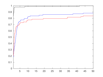
Figure 1: Performance profile for deterministic OFFO algorithms on noiseless OPM problems: AR2 (black), OFFAR2a (red) and OFFAR2b (blue)

	AR2	OFFAR2a	OFFAR2b
$\pi_{\tt algo}$	0.99	0.78	0.83
$\rho_{\tt algo}$	97.48	81.51	88.24

Table 2: Performance and reliability statistics on OPM problems without noise

Obviously, if we were to consider noiseless problems only, there would be little motivation (beyond theoretical curiosity) to consider the OFFAR2 algorithms. This is not unexpected since AR2 does exploit objective function values and we know that identical global convergence orders may not directly translate into similar practical behaviour. We nevertheless note that the global behaviour of the OFFAR2 algorithms is far from poor on reasonably well-conditioned cases.

However, as we have announced, the situation is quite different when considering the noisy case. When noise is present and because the value of $\mu_{1,k}$ (which is crucial to the performance of the OFFAR2 algorithnm) directly depends on the now noisy gradient, we have modified (2.8) slightly in an attempt to attenuate the impact of noise. We then use the smoothed update

$$\delta_{k}=\frac{9}{10}\delta_{k-1}+\frac{1}{10}\left(\frac{2\|g_{k}\|}{\|s_{k-1}\|^{2}}\right),\;\;\;\;\mu_{1,k}=\delta_{k}-\theta_{1}\sigma_{k-1},$$

where $\delta_{0}=\max[\varsigma,\|g_{0}\|]$, instead of (2.8). Similarly we use a smoothed version of the gradient’s norm

$$\tau_{k}=\frac{9}{10}\tau_{k-1}+\frac{1}{10}\|g_{k}\|$$

(with $\tau_{-1}=\|g_{0}\|$) instead of $\|g_{k}\|$ in (5.1) and (5.2).

Table 3 shows the reliability score $\rho_{\tt algo}$ of the three algorithms for four increasing percentages of relative random Gaussian noise added to the derivatives (and the objective function for AR2), averaged over 10 runs. The tolerance $\epsilon_{1}$ was set to $10^{-3}$ for these runs.

	$5\%$	$15\%$	$25\%$	$50\%$
AR2	40.67	30.84	24.54	6.81
OFFAR2a	80.76	75.38	70.76	56.30
OFFAR2b	85.97	80.67	72.69	47.98

Table 3: Reliability statistics $\rho_{\tt algo}$ for 5%, 15%, 25% and 50% relative random Gaussian noise (averaged on 10 runs)

As anounced, the reliability of AR2 decreases sharply when the noise level increases, essentially because the decision to accept or reject an iteration, which is based on function values, is strongly affected by noise. By contrast, the reliability of the OFFAR2 variants decreases remarkably slowly, especially for the OFFAR2a variant (using the more conservative $\beta=1$). That this variant is able to solve more that 50% of the problems with 50% relative Gaussian noise is quite encouraging.

6 Conclusions and Perspectives

We have presented an adaptive regularization algorithm for nonconvex unconstrained minimization where the objective function is never calculated and which has, for a given degree of used derivatives, the best-known worst-case complexity order, not only among OFFO methods, but also among all known optimization algorithms seeking first-order critical points. In particular, the algorithm using gradients and Hessians requires at most ${\cal O}(\epsilon_{1}^{-3/2})$ iterations to produce an iterate such that $\|\nabla_{x}^{1}f(x_{k})\|\leq\epsilon_{1}$, and at most ${\cal O}(\epsilon_{2}^{-3})$ iterations to additionally ensure that $\lambda_{\min}[\nabla_{x}^{2}f(x_{k})]\geq-\epsilon_{2}$. Moreover, all stated complexity bounds are sharp.

These results may be extended in different ways, which we have not included in our development to avoid too much generality and reduce the notational burden. The first is to allow errors in derivatives of orders 2 to $p$. If we denote by $\widehat{\nabla_{x}^{i}f}$ the approximation of $\nabla_{x}^{i}f$, it is easily seen in the proof of Lemma 3.4 that the argument remains valid as long as, for some $\kappa_{D}\geq 0$,

$$\|\widehat{\nabla_{x}^{i}f}(x_{k})-\nabla_{x}^{i}f(x_{k})\|\leq\kappa_{D}\|s_{k}\|^{p+1-i}.$$ (6.1)

Since, for first-order analysis, the accuracy of derivatives of degree larger than one only occurs in this lemma, we conclude that Theorem 3.10 still hold if (6.1) holds.

The second extension is to replace the Euclidean norm by a more general (possibly non-smooth) norm in $\hbox{I\hskip-2.0ptR}^{n}$. As in [24], this can be achieved without modification if first-order points are sought. When searching for second-order points, the second-order optimality measure $\min_{\|d\|=1}\nabla_{x}^{2}f(x_{k})[d]^{2}$ must then be used instead of $\lambda_{\min}[\nabla_{x}^{2}f(x_{k})]$.

The third extension is to weaken the gradient Lipschitz continuity in AS.3 by only asking Hölder continuity, namely that there exist non-negative constant $L_{p}$ and $\beta\in(0,1]$ such that

$$\|\nabla_{x}^{p}f(x)-\nabla_{x}^{p}f(y)\|\leq L_{p}\|x-y\|^{\beta}\,\text{ for all }x,y\in\hbox{I\hskip-2.0ptR}^{n}.$$ (6.2)

It then possible to verify that all our result remain valid with $p+1$ replaced by $p+\beta$.

Further likely generalizations include optimization in infinite-dimensional smooth Banach spaces, a development presented for the standard framework in [20]. This requires specific techniques for computing the step and a careful handling of the norms involved. We may also consider imposing convex constraints on the variables [11, Chapter 6]. An extension to guarantee third-order optimality conditions (in the case where third derivatives are available) may also be possible along the lines discussed in [11, Chapter 4].

We also observe that the lower bound $\sigma_{k}\geq\max[\mu_{1,k},\mu_{2,k}]$ has not yet, to the best of our knowledge, been used in implementations of the standard AR2 algorithm. Its incorporation in this method is clearly possible and worth investigating.

Given the prowess of OFFO methods on noisy problems, the transition from the present deterministic theory to the noisy context is clearly of interest and is the object of ongoing research. More extensive numerical experiments involving both regularization and trust-region methods using a variety of approximate derivatives are beyond the scope of this paper and will be reported separately.

References

[1]
S. Bellavia, G. Gurioli, B. Morini, and Ph. L. Toint.
A stochastic ARC method with inexact function and random
derivatives evaluations.
In Proceedings of the International Conference on Machine
Learning (ICML2020), 2020.
[2]
S. Bellavia, G. Gurioli, B. Morini, and Ph. L. Toint.
Quadratic and cubic regularization methods with inexact function and
random derivatives for finite-sum minimization.
In Proceedings of the ICCSA 2021, 2021.
[3]
S. Bellavia, G. Gurioli, B. Morini, and Ph. L. Toint.