Formally Modeling Autonomous Vehicles in LNT for Simulation and Testing

Abstract

We present two behavioral models of an autonomous vehicle and its interaction with the environment. Both models use the formal modeling language LNT provided by the CADP toolbox. This paper discusses the modeling choices and the challenges of our autonomous vehicle models, and also illustrates how formal validation tools can be applied to a single component or the overall vehicle.

1 Introduction

Autonomous vehicles (AV) are complex safety critical systems, as undesired behaviours can lead to fatal accidents [2]. Both the complete AV and its components need to be tested to handle critical scenarios. Because these critical scenarios are unlikely to happen in real environments, a common practice in robotics [20] is to reproduce these critical scenarios in an autonomous driving (AD) simulator, such as CARLA [6]. The specifications of these critical scenarios are obtained manually, by random generation, or by derivation from a (formal) model [7, 19, 10].

The main contributions of this paper are (a) two formal models of an AV and its environment, which can be used to generate relevant critical scenarios for testing AVs and/or their components, and (b) a discussion comparing the models and motivating the existence of two different models by their intended principal uses. Both models describe an autonomous ego vehicle, called car, moving around in a scene, called (geographical) map, towards a goal or destination position, and interacting with its environment, i.e., a given set of moving obstacles (pedestrians, cyclists, other cars, etc.) to avoid collisions. The formal models are written in the LNT language [9, 4], which is the most recent modeling language supported by the CADP verification toolbox [8] and a state-of-the-art replacement for the international standards LOTOS and E-LOTOS [9]. We chose LNT rather than a scenario modeling language such as Scenic [7] to illustrate a model-based, formal verification and testing approach [17, 10]. The first formal model specifies the control of the car (including route planning), considering an abstract representation of the geographical map as a graph. The second model focuses on the perception components of the car, and therefore it does not need to include a specification of the vehicle’s control, but requires a refined, more precise representation of the map. Both models were not yet fully disclosed.

We validated both models using different approaches supported by the CADP tools. First, we checked several safety and liveness properties characterizing the correct behavior of an AV. Concretely, we expressed the properties in the MCL [18] data-handling, action-based temporal property language, and verified them on the models using the on-the-fly model checker of CADP. Second, we generated several relevant AD scenarios from the models. More precisely, we used TESTOR [16], a tool developed on top of CADP for on-the-fly conformance test case generation guided by test purposes, to generate abstract test cases, which were automatically translated into AD scenarios [10].

The rest of this paper is organized as follows. Section 2 presents the first formal model of an AV, including its control, and the validation of the model using safety and liveness properties. Section 3 presents the second formal model of an AV, with a refined map, and generation of AD scenarios based on the model. Section 4 compares both models and gives concluding remarks. Appendices A and B give the complete LNT source code of the first and second model, respectively.

2 Model focused on control

Figure 1: Architecture of the autonomous vehicle LNT model focused on control

Arrows indicate messages sent between components and arrow labels denote the gates used.

In the first model, the autonomous car itself consists of four components: a GPS, a radar, a decision (or trajectory) controller, and an action controller. We chose these four components in order to represent the essential functionalities present in an autonomous car: perception (GPS and radar), decision, and action. The GPS keeps the current position of the car updated. The radar detects the presence of the obstacles close to the car and builds a perception grid summarizing information about perceived obstacles. The decision controller computes an itinerary from the current position to the destination, avoiding streets containing obstacles. The action controller commands the engine and direction to follow the itinerary computed by the decision controller, using the perception grid built by the radar to avoid collisions. As shown in Figure 1 these four components communicate in various ways: the GPS sends the current position to the decision controller upon request, the radar periodically sends the perception grid to the action controller, and the action controller requests a new itinerary from the decision controller. This LNT model is a translation of the GRL model [14, Appendix B] used to illustrate the combination of synchronous and asynchronous test generation tools [15] to validate GALS (Globally Asynchronous, Locally Synchronous) systems.

2.1 Elements and processes composing the model

The car has an initial position and a destination. Each obstacle has an initial position and a list of moves. The model’s behavior is defined such that inevitably either the car arrives, a collision occurs between the car and an obstacle, or all obstacles finish their list of moves. The LNT model is generic and is instantiated for a particular scene by providing global constants for the map, the initial position and destination of the car, and the set of obstacles with their initial positions and lists of moves.

Car.

Each component of the car is specified as a LNT process, and a process CAR defines the overall behavior as the parallel composition of these four processes (PERCEPTION_RADAR, PERCEPTION_GPS, DECISION, and ACTION) as shown in the following LNT fragment (the visible gates of a process are specified between square brackets “[…]”; a process must synchronize on the gates before the arrow “->”):

⬇

par

CURRENT_GRID ->

PERCEPTION_RADAR [UPDATE_GRID, CURRENT_GRID]

||

REQUEST_POSITION, CURRENT_POSITION ->

PERCEPTION_GPS [UPDATE_POSITION, REQUEST_POSITION, CURRENT_POSITION]

||

REQUEST_PATH, CURRENT_PATH, REQUEST_POSITION, CURRENT_POSITION ->

DECISION [REQUEST_PATH, CURRENT_PATH, REQUEST_POSITION,

CURRENT_POSITION, ARRIVAL] (map, destination)

||

CURRENT_PATH, CURRENT_GRID, REQUEST_PATH ->

ACTION [REQUEST_PATH, CURRENT_PATH, CURRENT_GRID,CAR_MOVE,COLLISION]

end par

Car components.

The LNT process PERCEPTION_RADAR has two local variables to keep track of the current and previous perception grid. A perception grid is represented by a list of edges corresponding to the streets occupied by the obstacles. This grid is initially empty (i.e., it has the value Radar ({})). After each obstacle or car move, the radar receives the current grid as a message from the environment, but informs the driving controller only in case of a change.

The LNT process PERCEPTION_GPS initializes the car position, receives updates of the car position (on gate UPDATE_POSITION) and position requests from the decision controller (on gate REQUEST_POSITION). Upon request, it sends the car position to the decision controller (on gate CURRENT_POSITION).

The LNT process DECISION has two value parameters: the initial map and the destination of the car. Process DECISION waits for receiving from process ACTION (on gate REQUEST_PATH) a request to compute a path avoiding obstacles, then requests the current position from process PERCEPTION_GPS (on gate REQUEST_POSITION). When process DECISION receives the current position (on gate CURRENT_POSITION), it checks if the car arrived at the destination, in which case it performs a rendezvous on gate ARRIVAL and stops; otherwise it computes an itinerary (using classical graph exploration algorithms) and sends it to process ACTION (on gate CURRENT_PATH). An itinerary is a list of controls, i.e., a turn in one of the crossroads (turned_n (N: Nat)) or a brake (brakes). If there is no possible itinerary avoiding the obstacles, an empty itinerary is sent (if the obstacles have finished their moves, this leads to a deadlock).

The LNT process ACTION requests an itinerary avoiding the obstacles from process DECISION (on gate REQUEST_PATH), and then it checks if the itinerary is feasible: if yes, it moves the car according to the first control in the itinerary (e.g., turn in the 5th crossroad), if not it waits for obstacles moves. Finally, after each perception change received from process PERCEPTION_RADAR, it requests a new itinerary with the updated list of obstacle positions (on gate REQUEST_PATH).

Geographical map.

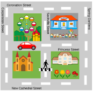
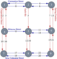
(A) Map (with the car and a crossing pedestrian)	(B) Map representation as directed graph

Figure 2: Example of a geographical map and its corresponding graph representation

The geographical map is represented as a directed graph as illustrated in Figure 2.B, in which edges correspond to streets and nodes correspond to crossroads; for simplicity, we assume that an actor (car or an obstacle) occupies a street completely (a longer street can be represented by several edges in the graph). A set of functions is defined to explore this graph, to compute itineraries, etc. The example below shows a a fragment of the LNT constant initial_map that returns the graph corresponding to the map illustrated on Figure 2.

⬇

function initial_map : Graph is

var g: Graph, e: Edges, v: Vertices in

v := {0, 1, 2, 3, 4, 5, 6, 7, 8};

e := {Edge (0, Coronation_Street, 1),

Edge (0, Corporation_Street, 3),

Edge (1, Coronation_Street_bis, 0),

... };

g := Graph (v, e);

return g

end var

end function

Obstacles.

As the car, obstacles move from a street-segment to an (adjacent) street-segment. If an obstacle is on the same segment as the car, this corresponds to a collision. To limit the complexity, each obstacle executes a fixed number of random or statically chosen moves. More precisely, there are three types of obstacle moves: (1) the obstacle can either leave, (2) turn in one of the crossroads, or (3) perform a random move. These moves are defined by the following LNT type Operation.

⬇

type Operation is – obstacle operations

random,

turned_n (N: Nat),

leave

end type

The behaviour of an obstacle is specified in the process OBSTACLE. It consists of executing the sequence of the obstacle’s moves and then stop. The first move corresponds to the appearance of the obstacle at its initial position. For random, the next move is chosen randomly among those possible in the current map (e.g., leave or turn (0)) as shown in the following LNT fragment of the process OBSTACLE.

⬇

if opi == random then

select

opi := leave

[] var n0, n1: Nat in

n1 := length (succ_l (map.G.E, o.position));

n0 := any Nat where n0 <= n1;

opi := turned_n (n0)

end var

end select

end if;

Note that the LNT operator select specifies non-deterministic choice. Finally, when the next move is chosen, the obstacle only executes the move if the destination segment is free; otherwise, it waits. Note that the process OBSTACLE receives from the process ENVIRONMENT updates of the positions of the car and obstacles. The LNT process OBSTACLES_MANAGER groups several obstacles in a parallel composition, providing the initial list of moves to each obstacle.

Map management.

The map is akin to a global variable modified at each move of the car or an obstacle. The updates of the map are handled by the process MAP_MANAGEMENT, which ensures that: (1) the geographical map information, such as the position of the car (map.c) and obstacles (grid), is shared with the process RADAR (by sending this information to RADAR on gate POSITIONS); (2) the geographical map information is updated when the car or the obstacles move (by receiving these moves from the processes ACTION and RADAR); and (3) the processes can only be executed as long as the car did neither arrive at destination nor crash, and at least one obstacle has still some moves to execute. The environment is defined as the parallel composition of the process OBSTACLES_MANAGER and MAP_MANAGEMENT in the process ENVIRONMENT.

2.2 Module hierarchy and scenario module

The model is split in three different parts. First, a part with definitions independent of the AV, e.g., types related to graph definitions together with the classical graph functions. Second, a generic part, defining types, functions, and processes common to all configurations. Finally, a particular part, defining the constants characterizing the considered configuration: the geographical map, the number of obstacles, as well as the initial position and behaviour of these obstacles.

Stats.

The resulting LNT specification has 881 lines dispatched in four modules, containing 14 types, 19 functions, six channels, and ten processes. Using CADP, for the map with 22 streets and 8 crossroads represented in Figure 2 and two obstacles, each with one random move, we generated (in about a minute on a standard laptop) the corresponding LTS (Labelled Transition System): 59,781 states and 179,884 transitions (13,305 states and 28,601 transitions after strong bisimulation minimization).

2.3 Validation by model checking

We validated our LNT model by checking several safety and liveness properties characterizing the correct behavior of the AV. We expressed the properties in MCL [18], the data-handling, action-based, branching-time temporal logic of the on-the-fly model checker of CADP. We describe here two properties in natural language and in MCL—more were verified for the associated GRL model [15].

Property 1:

“The position of the car is correctly updated after each move of the car.” This safety property expresses that on each transition sequence, an update of the car position (“UPDATE_POSITION ?current_street”, where current_street is the street on which the car currently is) followed by a car move (“CAR_MOVE ?control”, where control is a move) cannot be followed by an update of the car position inconsistent with current_street, control, and the map. This can be expressed in MCL using the necessity modality below, which forbids transition sequences containing inconsistent position updates:

⬇

[ true* .

{ UPDATE_POSITION ?current_street:String } .

(not ({ CAR_MOVE ... } or { UPDATE_POSITION ... }))* .

{ CAR_MOVE ?control:String } .

(not ({ CAR_MOVE ... } or { UPDATE_POSITION ... }))* .

{ UPDATE_POSITION ?new_street:String where

not (Consistent_Move (current_street, control, new_street)) }

] false

The values of the current position, the move, and the new position of the car occurring as offers for the gates UPDATE_POSITION and CAR_MOVE are captured in the variables current_street, control, and new_street of the corresponding action predicates (surrounded by curly braces) and reused in the where clause of the last action predicate. The Boolean function Consistent_Move defines all valid combinations for current_street, control, and new_street allowed by the map.

Property 2:

“Inevitably, the system should reach a state where either the car arrived (ARRIVED), or a collision occurred between the car and an obstacle (COLLISION), or all obstacles have finished their list of moves (END_OBSTACLE).” This property can be expressed in MCL using the formula below, which forbids infinite transition sequences not containing one of the three terminal actions (TERMINATE):

⬇

not <(not TERMINATE)>@

Here, TERMINATE encompasses all three terminal actions ARRIVED, COLLISION, and END_OBSTACLE. Note that this formula correctly expresses the property if and only if the model is free of deadlocks, which can be easily verified by another check.

Note that we also specified test purposes and generated test cases from this model using TESTOR [16] as part of the evaluation of a test generation approach [17].

2.4 Discussion

We specified an AV close to a deployed one, i.e., we considered an AV as consisting of several components for action, decision, and perception. To naturally specify the search of an itinerary, we represented the geographical map as a graph, and formalized classical graph exploration algorithms. This model is a translation of a GALS model [15, 14] previously described in the formal GRL language [13, 12], where the various components of the car are represented as synchronous programs interacting globally in an asynchronous manner.

This first model can directly be used to test the control of an AV, since it computes the possible itineraries avoiding collisions. However, the abstraction of each component can be refined according to different evaluation goals. For instance, to only test the perception component (e.g., radar) the current formal model is too general and the current abstraction of the map is not optimal to verify a perception component. In particular, more precision is required for the geographical map (e.g., concrete angles and lengths of street segments) and (the trajectories of) obstacles (e.g., their size and speed). On the other hand, some information might not be necessary to test a particular component (e.g., the control and action processes might be irrelevant to test the perception): thus, these aspects can be dropped from the model, consequently improving validation performance by reducing the size of the underlying LTS.

In the next section, we will present a second formal model for an AV. If the overall structure of the second model is the same (in particular the module hierarchy and the processes OBSTACLES_MANAGER and MAP_MANAGEMENT), the second model focuses on the perception component, which requires a more precise representation of the geographical map.

3 Model focused on perception

To validate the perception components, which are crucial for an AV, it is necessary to devise a model focused on perception aspects. We present below such a model in LNT, derived from the control-focused model given in Section 2. This second model keeps the same management of actors and important events (arrival of the car at destination, end of obstacle trajectories, and collision), but represents the map using an array instead of a graph, and abstracts away most car components, except for the perception LiDAR. This perception-focused model was used to generate scenarios to be executed on an AD simulator.

3.1 Elements and processes composing the model

Figure 3: Architecture of the autonomous vehicle LNT model focused on perception

Constants and Channels.

The principal constants are the height and width of the array defining the map, and those of the array defining the perception grid of the LIDAR component. They are mostly used to verify if an actor is present on the map or not. The default size of the map is ten$\times$ten cells, and it can be increased for a higher resolution. The various processes in the model communicate through gates defined with channels used to convey specific data values. We defined seven different channels in the model.

Obstacles.

The obstacles are actors on the map that represent various objects and elements of the environment. Obstacles can have various sizes (minimum one cell) as they can be pedestrians, cars, or buildings. Each obstacle has a unique identifier defined as a value of an enumerated type. Obstacles can be static or mobile, the latter ones being able to move in any direction. Each move consists in traversing a number of cells determined by the obstacle speed. Some obstacles can hide the view (e.g., a car or a building) and some cannot (e.g., a pedestrian or a pole).

In a configuration, each obstacle has a list of moves defining its behavior. Its moves depend on its speed and direction. An obstacle may also choose not to move or may randomly choose between several possible directions, which adds nondeterminism to the model and enables the exploration of further scenarios. As in the first model, obstacle moves must not lead to collisions (i.e., end on occupied cells of the map) in order to yield relevant scenarios. To keep the model size tractable, we enable full random moves only for obstacles close enough to the car, the random moves of the farther obstacles being restricted to directions bringing them closer to the car.

Each obstacle is modeled by an instance of the OBSTACLE process, which has as parameters the obstacle’s identifier, its list of moves, and a flag indicating whether the obstacle has a cyclic movement. Before attempting the next obstacle move (at the head of the list), process OBSTACLE obtains, via gate GRID_UPDATE, the current map from the MAP_MANAGER process. Based on the map, on the current obstacle information (position and speed), and on the direction of the next move, the obstacle determines whether the move is valid, i.e., does not lead to a collision. Then, process OBSTACLE sends on gate OBSTACLE_POSITION the previous position, next position, and new direction of the obstacle (including the case when the obstacle does not move) to process MAP_MANAGER, in charge of updating the map. If the next direction of move is random, the possible moves of the obstacle are constrained by the RESTRAND process, described later in this section. When the list of moves is finished, process OBSTACLE performs an END_OBSTACLE action and stops moving, except when it has a cyclic behaviour, in which case it starts again using its list of moves given initially. The process OBSTACLES_MANAGER is the parallel composition of all OBSTACLE processes in the considered configuration.

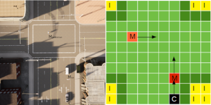
Figure 4: Representation of the map with three actors (car and two mobile obstacles)

Map.

The map is essentially the representation of the ground truth, the world in which the different actors move. The map is represented as a 2–dimensional array composed of cells with different values: free when there is no obstacle nor car on the cell, occupied (obstacle) when the cell is occupied by an obstacle (including all the obstacle information), and car_pos when the cell is occupied by the car (we consider only one car on the map). The map is defined and initialized in LNT as follows:

⬇

type Map_Info is free, car_pos, occupied (O:Obstacle) end type

type Map_Line is array [0..9] of Map_Info end type

type Map is array [0..9] of Map_Line end type

function initiate_map (out var m:Map) is

– create an empty map

m := Map (Map_line (free));

– add static obstacles into the ground truth array

add_obstacle (!?m, Obstacle (Scenery,

CellRectPosition (Position (0, 0)),

Obstacle_Speed (0), none, false));

...

– add mobile obstacles into the ground truth array

add_obstacle (!?m, Obstacle (Other_Car,

CellRectPosition (Position (6, 7)),

Obstacle_Speed (1), up, false));

...

end function

The MAP_MANAGER process is a central part of the model, in charge of maintaining the map (ground truth) and of communicating with the other processes to update the position of the actors. The map is initialized with the positions of static obstacles and the initial positions of mobile obstacles. It is sent on gate GRID_UPDATE to the OBSTACLE processes to determine their next moves, and is also sent on gate GRID_CAR (accompanied by the car position) to the process LIDAR_MANAGER to generate the perception grid. If at some moment the position of the car becomes the same as one of the obstacles, MAP_MANAGER performs an action COLLISION and stops, entailing the termination of the whole scenario. The ENVIRONMENT process is the parallel composition of MAP_MANAGER and OBSTACLES_MANAGER.

Car.

The CAR process is the parallel composition of the LIDAR_MANAGER and CAR_MOVE processes, the latter being in charge of managing the car moves. Process CAR_MOVE has as parameters the car’s information (position, list of moves, speed, and a flag indicating if the car has a cyclic movement) and is similar to process OBSTACLE. The car moves essentially in the same way as the obstacles, except that it can also move to an occupied cell, and thus trigger a COLLISION action from the GRID_MANAGER process. Upon each move of the car, its previous and current positions are transferred to the MAP_MANAGER process on gate CAR_POSITION to be updated on the map. If the car has finished its list of moves, it performs an action ARRIVAL, which terminates the scenario.

LiDAR.

The perception grid represents the perception of the car (as computed by the LiDAR) up to a certain distance. It is modeled as a 2-dimensional array centered on the car position and having a default size of 5x5 cells. The cells of the perception grid have different values from those of the map: F for free cells, C for the car position, O for occupied cells, M for cells that were free on the last grid but became occupied, T for cells occupied by a transparent obstacle, N similar to M but for cells occupied by transparent obstacles, and U for unknown cells, i.e., those out of the map (if the grid exceeds the map boundaries) or those hidden from view (behind an opaque obstacle). The perception grid is defined as follows and initialized as an empty array:

⬇

type Perception_Info is C, F, O, M, T, N, U end type

type L is array [0..4] of Perception_Info end type

type P is array [0..4] of L end type

There are several functions calculating the perception grid. The principal one takes the map, the previous perception grid and the current position of the car to calculate the new grid by translating the values of map cells into the values of the corresponding grid cells. Other functions calculate the hidden cells depending on the presence of opaque obstacles around the car, and update the value of grid cells from F to M or to N if these changed between two consecutive grids. The perception grid is maintained by the LIDAR_MANAGER process, which sends on gate LIDAR_MAP the new value of the grid and map to process MOVE_CAR to compute the next car moves. Process LIDAR_MANAGER also has a special parameter to indicate whether the contents of the grid must be kept available in the LTS for validation purposes.

Scheduler and Restrand.

Two auxiliary processes optimize the model regarding both its scalability and its realism when connected to an AD simulator. The SCHEDULER process introduces additional synchrony in the model to bring it closer to its physical counterpart, by enforcing that between two consecutive time instants, every actor must perform one move (at its own speed). Process SCHEDULER monitors the moves of the car and the obstacles by synchronizing on gates CAR_POSITION and OBSTACLE_POSITION, indicates consecutive time periods by emitting signals on a special gate TICK, and forces all actors (in a fixed order) to perform one move between two TICK actions (note that an obstacle may choose not to move, which amounts to keep its position unchanged). This improves the execution of transition sequences in the AD simulator, by allowing all actor moves between two TICK actions to be performed in parallel, yielding realistic movements, as opposed to jerky ones induced by equivalent, but less realistic interleavings in the absence of TICK actions. This also reduces the size of the LTS by pruning redundant interleavings of actions (equivalent orderings of obstacle moves between two TICK actions). Between two TICK actions, the car moves after all obstacles, because at the end of the scenario (car arrival or a collision), the obstacles must still be able to finish their moves in the simulator.

⬇

process SCHEDULER [OBSTACLE_POSITION:O, CAR_POSITION:C, TICK:none] is

loop

OBSTACLE_POSITION (?Obstacle (Pedestrian, any RectPosition,

any Obstacle_Speed, any Direction, true),

?any Obstacle, ?any Direction);

... – all the other obstacles

CAR_POSITION (?any Position, ?any Position);

TICK

end loop

end process

The RESTRAND (for “restraining random”) process limits the random moves of the obstacles to keep them in a meaningful neighbourhood of the car. This is useful both for specifying scenarios with relevant obstacle trajectories (obstacles close enough to be perceived by the LiDAR) and for reducing the LTS. Process RESTRAND monitors the obstacle moves by synchronizing on gate OBSTACLE_POSITION and constrains the random moves (depending on the car position, the previous obstacle position, a direction and the minimal distance) to force obstacles to get close enough to the car to be perceived.

⬇

OBSTACLE_POSITION (?any Obstacle, ?any Obstacle, dir)

where dir != random

[] OBSTACLE_POSITION (?obst, ?obst_prev, random)

where moveAllowed (car, obst_prev, obst.dir, distMin)

3.2 Module hierarchy and scenario module

The LNT model is structured as a hierarchy of modules, depending on the type of data the functions or processes work on. All type definitions are grouped in the top module of the hierarchy, which is then separated in two branches, one for the modules concerning the environment (obstacles, map) and the other for the modules concerning the car. The main module inherits from both branches.

The modules are the following: types contains the data types, constants, and generic functions; lidar contains the functions and the process for the perception grid; car defines the behaviour of the car; map contains the functions for updating the map; obstacles contains the functions and processes to move obstacles; scenario contains the definitions specific to a configuration; map_manager contains the process monitoring the map; finally, the main module contains the parallel composition of the principal processes.

To easily build various configurations of the LNT model, the scenario module enables to choose the map, the initial positions of (static and dynamic) obstacles, and the behaviour of the car. The only parameter not defined in the scenario module is the size of the map, defined in the types module because of the hierarchy. The example SCENARIO given in Appendix B contains four static obstacles and two moving obstacles (another car and a pedestrian) with a simple trajectory. We decided to place the processes RESTRAND and SCHEDULER in the scenario module because these processes depend on the number of obstacles and, for RESTRAND, on the distance from the car that is chosen for randomly moving obstacles.

Stats.

The resulting LNT specification has 1059 lines (excluding the scenario module, the size of which depends on the configuration—the one given in Appendix B has 161 lines) dispatched in eight modules, containing 13 types, 38 functions, seven channels, and eleven processes. Using CADP, for the map of size ten$\times$ten represented in Figure 4 and two obstacles, we generated (in less than a minute on a standard laptop) the corresponding LTS with 27,168 states and 50,719 transitions (14,595 states and 28,287 transitions after strong bisimulation minimization).

3.3 Test case generation for simulation scenarios

The model focused on perception was devised for the synthesis of AD simulation scenarios from conformance test cases generated using the TESTOR [16] tool, as reported in [10]. The model was first validated by checking several temporal logic properties expressed in MCL [18].

The generation of test cases is guided by test purposes, which are high-level descriptions of the sequences of actions to be reached by testing. A test purpose is an LNT process specifying a sequence of actions terminated by a TESTOR_ACCEPT action characterizing the desired situation. An example of test purpose defining a sequence of (zero or more) actions leading to a COLLISION is given below.

⬇

process PURPOSE [TESTOR_ACCEPT: none, COLLISION: COLLISION_O] is

COLLISION (Pedestrian);

loop TESTOR_ACCEPT end loop

end process

We tested the model with ten different configurations, on three different maps, with three different test purposes. The first configuration was the one represented on Figure 4. On a crossroad, a car (moving obstacle) is going straight to the north, the car is following it, and a pedestrian is trying to cross and walk between them. The two different outcomes defined in test purposes are that a collision happens or not. Three other configurations were variants of this one on the same map. In two other configurations, the obstacles do not have defined trajectories, their moves being specified in the test purpose (reaching a collision or a particular perception grid). Another configuration involved a map representing a highway where three vehicles (including the car) move at different speeds in the same direction and try to change the lane. A further configuration involved a T-shaped crossroad, where another vehicle ignores the signalisation, leading to a collision with the car. Finally, we specified two configurations containing an additional obstacle that may produce near misses, where the car would be just next to an obstacle but not collide with it.

3.4 Discussion

This second model focuses on a particular component (i.e., the perception), with a more precise representation of the geographical map. The advantage of this focus is the possibility to refine the precision of the moves of the obstacles and the car (e.g., by increasing the resolution of the map and perception grid) and to fine-tune the model to cover a large number of relevant AD perception scenarios. For instance, this model enables random trajectories for the obstacles with different speeds around the car, within an area of parameterized size managed by the RESTRAND process. Although the second model focuses on the perception component, (re)integrating a control component could enrich the car’s trajectory, which also impacts the perception in AD scenarios. However, a simple control component computing a random trajectory (or executing a precomputed one) for the car would be sufficient.

4 Conclusion

Existing work in formal models of autonomous driving (AD) systems focuses either on modelling one component in particular as in [11], or on verifying a given AD scenario as in [5], where a DSL is proposed to specify AD scenarios, which are subsequently translated into networks of stochastic hybrid automata and are verified using the UPPAAL-SMC model checker [3].

In contrast, we presented two formal LNT models specifying the interaction of an AV with its environment, for the purpose of generating AD scenarios and testing the vehicle or some of its components in an deployment environment. Our first model is more general, i.e., consists of a higher abstraction of both the AV and the environment, and includes several components (perception, decision, action) of the AV, whereas our second model focuses more on a particular component of the vehicle (i.e., the perception component) and considers a fragment of the geographical map, which results in a more refined representation of both the component and the geographical map representation. Both models can be and have been used to test AVs: the first one to generate tests for the entire system, which does not require a refined abstraction of each AV component, and the second one to generate tests for validating a particular perception component, which requires a more precise representation of the map.

As future work, we plan to unify both models. This could be beneficial for the generation of more refined test cases, i.e., including the control of the car on a precise fragment of the geographical map. We then plan to transform these refined test cases into scenarios for an AD simulator such as CARLA, using the approach of [10]. Finally, we plan to take advantage of both the refined test cases and the corresponding derived AD scenario to test the control component using online conformance testing techniques.

Acknowledgments. This work was partly supported by project ArchitectECA2030 that has been accepted for funding within the Electronic Components and Systems for European Leadership Joint Undertaking in collaboration with the European Union’s H2020 Framework Programme (H2020/2014-2020) and National Authorities, under grant agreement No. 877539.

Appendix A Full model focused on control

This appendix presents the first LNT model of the autonomous vehicle (AV) and its interaction with the environment. This model is fully self-contained and does not depend on any externally-defined library. For readability, the specification has been split into 8 parts, each part being devoted to a particular module, or a collection of test purpose. The first parts contain general definitions that could be independent of the autonomous vehicle; starting from Section A.2, the definitions become increasingly more AV-specific.

A.1 Definitions of generic graph functions and datatypes

The module graph_car defines the types related to graph definitions together with usual graph-exploration functions. This module is independent of the autonomous vehicle: for a use in another context, one only needs to replace the type Street by an appropriate type characterising edge labels, e.g., the generic type String or another type specific to a domain. The module clause with request the automatic definition of predefined functions for all types defined in the module.

⬇

module graph_car

with ==, !=, get, set, inter, union

is

————————————————————————

– Types

————————————————————————

type Street is

Coronation_Street,

Corporation_Street,

Coronation_Street_bis,

two_Coronation_Street,

Sackville,

two_Coronation_Street_bis,

Spring_Gardens,

Corporation_Street_bis,

Princess_Street,

two_Corporation_Street,

two_Princess_Street,

two_Sackville,

Spring_Gardens_bis,

two_Princess_Street_bis,

two_Spring_Gardens,

two_Corporation_Street_bis,

New_Cathedral_Street,

two_Sackville_bis,

New_Cathedral_Street_bis,

two_New_Cathedral_Street,

two_Spring_Gardens_bis,

two_New_Cathedral_Street_bis,

– obstacle labels:

Lily,

Theo,

HIDDEN

end type

————————————————————————

type Corner is

0,

1,

2,

3,

4,

5,

6,

7,

8

end type

————————————————————————

type Edge is

Edge (q1: Corner, l: Street, q2: Corner)

end type

————————————————————————

type Edges is

list of Edge

with head, tail, reverse, length, member

end type

————————————————————————

type Vertices is

list of Corner

with head, tail, member

end type

————————————————————————

type Graph is

– Digraph (directed graph)

Graph (V: Vertices, E: Edges)

end type

————————————————————————

– Functions

————————————————————————

function add_Edge (q1, q2: Corner, l: Street, e: Edges) : Edges is

– add (q1, l, q2) to e

return cons (Edge (q1, l, q2), e)

end function

————————————————————————

function succ_s (in var E: Edges, s: Corner) : Vertices is

– return targets of all edges in E leaving s

var list_succ: Vertices in

list_succ := {};

loop

case E

var q1, q2: Corner in

NIL ->

return list_succ

| CONS (Edge (q1, any Street, q2), E) ->

if q1 == s then

list_succ := cons (q2, list_succ)

end if

end case

end loop

end var

end function

————————————————————————

function succ_l (in var L: Edges, e: Edge) : Edges is

– return all edges of E that leave the target of e

var list_succ: Edges in

list_succ := {};

loop

case L

var q1, q2: Corner, s: Street in

NIL ->

return reverse (list_succ)

| CONS (Edge (q1, s, q2), L) ->

if q1 == e.q2 then

list_succ := add_Edge (q1, q2, s, list_succ)

end if

end case

end loop

end var

end function

————————————————————————

function succ_l_s (in var E: Edges, l: Street) : Corner is

– return target state of a succesor edge for a label

return edge_l (E, l).q2

end function

————————————————————————

function edge_l (in var E: Edges, l: Street) : Edge is

– return edge in E with label l

loop

assert E != {};

if head (E).l == l then

return head (E)

end if;

E := tail (E)

end loop

end function

————————————————————————

function is_l_in_E (in var E: Edges, l: Street) : Bool is

– return true iff there is an edge in E with label l

loop

case E

var l1: Street in

NIL ->

return false

| CONS (Edge (any Corner, l1, any Corner), E) ->

if l1 == l then

return true

end if

end case

end loop

end function

————————————————————————

function pred_edge (E: Edges, in var D: Edge) : Edges is

– return all edges of E that have the source of D as target

var pred, temp: Edges in

pred := {D};

temp := E;

loop L in

if temp == {} then

return pred

end if;

if (head (temp).q2 == D.q1) then

D := head (temp);

pred := cons (D, pred)

else

temp := tail (temp)

end if

end loop

end var

end function

————————————————————————

function delete_l_in_E (in var E: Edges, l: Street) : Edges is

– delete from E all edges with label l

var new: Edges in

new := {};

loop

case E

var q1, q2: Corner, l1: Street in

NIL ->

return new

| CONS (Edge (q1, l1, q2), E) ->

if l1 != l then

new := add_Edge (q1, q2, l1, new)

end if

end case

end loop

end var

end function

————————————————————————

function is_q1q2_in_E (in var E: Edges, A: Edge) : Bool is

– return true iff E has an edge with same source and target as A

loop

case E

var q1, q2: Corner in

NIL ->

return false

| CONS (Edge (q1, any Street, q2), E) ->

if (q1 == A.q1) and (q2 == A.q2) then

return true

end if

end case

end loop

end function

————————————————————————

end module

A.2 Definitions of AV specific datatypes

Using the types and functions defined in module graph_car (see Section A.1), the module types defines the AV specific datatypes together with their functions. It also defines the channels, i.e., the types of the offers exchanged during rendezvous.

⬇

module types (graph_car)

with ==, !=, get, set

is

————————————————————————

– Types

————————————————————————

type Localization is !printedby "PRINT_LOCALIZATION"

– global localization (perception of the GPS), annotated with the

– current position of the car

Localization (c: Edge, – current street (i.e., edge) of the car

G: Graph) – current state of the global map)

end type

————————————————————————

type Radar_Grid is

– local localization

– grid (obstacles or mvnt or nothing) (RADAR Grid)

– S0 initial states

Radar (E: Edges)

end type

————————————————————————

type Direction is

turn_n (N: Nat) – 5th if crossroads

end type

————————————————————————

type Itinerary is

– instruction list (– rename itinerary)

list of Direction

with head, tail, reverse

end type

————————————————————————

type Control is

– direction

turned_n (N: Nat),

brakes

end type

————————————————————————

type Obstacle is

Obstacle (name: Street, position: Edge)

end type

————————————————————————

type Operation is

– obstacle operations

random,

turned_n (N: Nat), – 5th if crossroads,

leave

end type

————————————————————————

type Obstacle_behaviour is

list of Operation

with head, tail

end type

————————————————————————

– Functions

————————————————————————

function succ_avoid_reach_D (E: Edges, P: Edge, D: Edge, avoid: Edges)

: Edges is

– compute successors leading to D avoiding the edges in a given list

var a: Edge, pred, succ, succ_t: Edges, dejavu: Vertices in

if member (P, E) == false then

return {}

end if;

a := P;

pred := {a};

succ := succ_l (E, a);

succ_t := succ;

dejavu := {a.q2};

loop

if member (D, succ_t) then

return pred_edge (pred, D)

elsif succ == {} then

return {}

else

a := head (succ);

succ := tail(succ);

if (member (a.q2, dejavu) == false) and

(member (a, avoid) == false) then

succ_t := succ_l (E, a);

pred := cons (a, pred);

succ := union (succ_t, succ);

dejavu := cons (a.q2, dejavu)

end if

end if

end loop

end var

end function

————————————————————————

function edges_to_itinerary (map: Localization, in var succ: Edges)

: Itinerary is

var eg: Edges, it: Itinerary, I: Nat in

it := {};

eg := map.G.E;

loop

if (succ == {}) or (eg == {}) then

return reverse (it)

end if;

if head (eg) == head (succ) then

I:= 0;

succ := tail (succ);

loop L in

if (succ != {}) then

eg := tail (eg);

if eg == {} then

eg := map.G.E

end if;

if head(eg).q1 == head (succ).q1 then

if head(eg).q2 == head (succ).q2 then

it := cons (turn_n (I), it);

break L

end if;

I := I + 1

end if

else

return it

end if

end loop;

eg := map.G.E

else

eg := tail (eg)

end if

end loop

end var

end function

————————————————————————

function compute_itinary (map: Graph, position, destination: Edge,

avoid: Edges)

: Itinerary is

– return if possible an itinerary leading from S to D in map

var succ: Edges in

succ := succ_avoid_reach_D (map.E, position, destination, avoid);

return edges_to_itinerary (Localization (position, map), succ)

end var

end function

————————————————————————

function car_controls (dir: Direction) : Control is

case dir

var N: Nat in

turn_n (N) -> return turned_n (N)

end case

end function

————————————————————————

function move_n (G: Graph, P: Edge, N: Nat) : Edge is

– return the car advancing in the n-th neighbourd

var eg: Edges, i: Nat in

eg := G.E;

i := 0;

loop L in

if eg == {} then

– no successor found: do not move

return P

end if;

if head (eg).q1 == P.q2 then

if i == N then

return head(eg)

else

i := i + 1

end if

end if;

eg := tail (eg)

end loop

end var

end function

————————————————————————

function move_car (map: Localization, action: Control) : Localization is

case action

var N: Nat in

turned_n (N) ->

return Localization (move_n (map.G, map.c, N), map.G)

| any ->

return map

end case

end function

————————————————————————

function move_obstacle (g: Graph, movement: Operation, o: Obstacle)

: Edge is

case movement

var N: Nat in

turned_n (N) -> return move_n (g, o.position, N)

| leave -> return Edge (0, HIDDEN,1)

| random -> return Edge (0, HIDDEN,1)

end case

end function

————————————————————————

function move_obstacle_grid (in var maj_radar: Radar_grid,

obst: Obstacle)

: Radar_Grid is

– return the same obstacle position exists

if is_q1q2_in_E (maj_radar.E, obst.position) then

return maj_radar

end if;

– delete the previous obstacle position

maj_radar := Radar (delete_l_in_E (maj_radar.E, obst.name));

– add the new obstacle position

return Radar (add_Edge (obst.position.q1, obst.position.q2,

obst.name, maj_radar.E))

end function

————————————————————————

function succ_edge (in var R: Radar_Grid, D: Edge)

: Radar_Grid is

– sucesseur of D

var succ: Edges, temp: Edge in

succ := {};

loop L in

if R.E == {} then

return Radar (succ)

end if;

temp := head (R.E);

if (temp.q1 == D.q2) then

succ := cons (temp, succ)

end if;

R := R.{E -> tail (R.E)}

end loop

end var

end function

————————————————————————

– Channels

————————————————————————

channel C is (c: Control) end channel

channel E is (e: Edges) end channel

channel G is (g: Radar_Grid) end channel

channel I is (i: Itinerary) end channel

channel O is (o: Obstacle) end channel

channel P is (e: Edge) end channel

————————————————————————

end module

A.3 Definitions for the autonomous vehicle

The four component of the autonomous car are defined as separate LNT processes PERCEPTION_RADAR, PERCEPTION_GPS, DECISION, and ACTION. These four components are composed in parallel in the process CAR and synchronize on their shared actions using the parallel composition operator.

⬇

————————————————————————

process PERCEPTION_RADAR [UPDATE_GRID, CURRENT_GRID: G] is

– local detection of obstacles

var current, previous: Radar_Grid in

UPDATE_GRID (?current);

previous := current;

CURRENT_GRID (current);

loop

– receive the current grid

UPDATE_GRID (?current);

– if the grid has changed, inform the driving controller

if current != previous then

CURRENT_GRID (current);

previous := current

end if

end loop

end var

end process

————————————————————————

process PERCEPTION_GPS [UPDATE_POSITION: P,

REQUEST_POSITION: none,

CURRENT_POSITION: P] is

– global localization

var current_street: Edge, pending_request: Bool in

– initialize the car’s position (i.e., the current street/edge)

UPDATE_POSITION (?current_street);

pending_request := false;

loop

select

– update the car’s position (i.e., the current street/edge)

UPDATE_POSITION (?current_street)

[]

– trajectory controller requests the position

REQUEST_POSITION;

pending_request := true

[]

– upon request, send the position to the trajectory controller

only if pending_request then

CURRENT_POSITION (current_street);

pending_request := false

end if

end select

end loop

end var

end process

————————————————————————

process DECISION [REQUEST_PATH: E,

CURRENT_PATH: I,

REQUEST_POSITION: none,

CURRENT_POSITION: P,

ARRIVAL: none]

(map: Graph, destination: Edge) is

var l_avoid: Edges, path: Itinerary, current_street: Edge in

loop

– wait for a request from the driving controller

REQUEST_PATH (?l_avoid);

– request the current position

REQUEST_POSITION;

CURRENT_POSITION (?current_street);

if current_street == destination then

– the car arrived to the final destination

ARRIVAL;

– stop

loop i end loop

end if;

– compute an itineray and send it to the driving controller

path := compute_itinary (map, current_street, destination,

l_avoid);

CURRENT_PATH (path)

end loop

end var

end process

————————————————————————

process ACTION [REQUEST_PATH: E,

CURRENT_PATH: I,

CURRENT_GRID: G,

CAR_MOVE: C,

COLLISION: P] is

var grid: Radar_Grid, path: Itinerary in

grid := Radar ({});

loop

– check feasibility of the itinerary

REQUEST_PATH (grid.E);

CURRENT_PATH (?path);

if path == {} then

– wait for the obstacles to move …

CURRENT_GRID (?grid)

else

loop L in

select

if path == {} then – last direction sent

break L

else

CAR_MOVE (car_controls (head (path)));

path := tail (path)

end if

[]

– receive the current local grid from the radar

– this branch should be prior than the previous one to

– never block the reception of a new grid from the radar

CURRENT_GRID (?grid);

break L

[]

COLLISION (?any Edge);

loop i end loop

end select

end loop

end if

end loop

end var

end process

————————————————————————

process CAR [UPDATE_GRID: G,

UPDATE_POSITION: P,

CURRENT_GRID: G,

REQUEST_POSITION: none,

CURRENT_POSITION: P,

REQUEST_PATH: E,

CURRENT_PATH: I,

CAR_MOVE: C,

ARRIVAL: none,

COLLISION: P]

(map: Graph, destination: Edge) is

par

CURRENT_GRID ->

PERCEPTION_RADAR [UPDATE_GRID, CURRENT_GRID]

||

REQUEST_POSITION, CURRENT_POSITION ->

PERCEPTION_GPS [UPDATE_POSITION, REQUEST_POSITION,

CURRENT_POSITION]

||

REQUEST_PATH, CURRENT_PATH, REQUEST_POSITION, CURRENT_POSITION ->

DECISION [REQUEST_PATH, CURRENT_PATH, REQUEST_POSITION,

CURRENT_POSITION, ARRIVAL] (map, destination)

||

CURRENT_PATH, CURRENT_GRID, REQUEST_PATH ->

ACTION [REQUEST_PATH, CURRENT_PATH, CURRENT_GRID, CAR_MOVE,

COLLISION]

end par

end process

————————————————————————

A.4 Definitions for the autonomous vehicles environment

The environment of the car is modeled by two LNT processes. First, the process OBSTACLE specifies the behaviour of an obstacle. Second, the process MAP_MANAGEMENT manages the ground truth, i.e., the positions of the car and obstacles on the map. Because many obstacles can be interacting with the AV, we added a third process OBSTACLES_MANAGER instantiating the number of obstacles, this process is presented in the next section. The MAP_MANAGEMENT and OBSTACLES_MANAGER processes are composed in the process Environment.

⬇

————————————————————————

process OBSTACLE [CAR_POSITION: P, OBSTACLES_GRID: G, OBSTACLE_MOVE: O]

(map: Localization,

o: Obstacle,

in var operations: Obstacle_behaviour) is

– execute the sequence of operations and then stop

var present: Bool, grid: Radar_grid, car_street: Edge in

present := false;

grid := Radar ({});

car_street := map.c;

loop

select

– apparition of the obstacle at its initial position

only if not (present or

is_q1q2_in_E (cons (car_street, grid.E),

o.position))

then

if member (o.position, map.G.E) then

OBSTACLE_MOVE (o);

present := true

end if

end if

[]

– movement of the obstacle

only if present and (operations != {}) then

var pos: Edge, opi: Operation in

opi := head (operations);

if opi == random then

select

opi := leave

[]

var n0, n1: Nat in

n1 := length (succ_l (map.G.E, o.position));

n0 := any Nat where n0 <= n1;

opi := turned_n (n0)

end var

end select

end if;

pos := move_obstacle (map.G, opi, o);

if is_q1q2_in_E (cons (car_street, grid.E),

pos) == false

then

OBSTACLE_MOVE (Obstacle (o.name, pos));

operations := tail (operations)

else

i – to avoid problems with the translation to LOTOS

end if

end var

end if

[]

– update the map with the current street of the car

CAR_POSITION (?car_street)

[]

– update the grid with the current position of the obstacles

OBSTACLES_GRID (?grid)

end select

end loop

end var

end process

————————————————————————

process MAP_MANAGEMENT [UPDATE_POSITION: P,

UPDATE_GRID: G,

CAR_POSITION: P,

OBSTACLES_GRID: G,

CAR_MOVE: C,

OBSTACLE_MOVE: O,

COLLISION: P]

(in global_loc: Localization) is

var map: Localization, grid: Radar_Grid, car_control: Control in

map := global_loc;

grid := Radar ({});

– initialize the position of the car: the map in the GPS does not

– change, thus send only the current street

UPDATE_POSITION (map.c);

loop

select

– handle car movement

CAR_MOVE (?car_control);

– compute car position and new grid for the radar

map := move_car (map, car_control);

– check if the car is in the same edge as an obstacle

if is_q1q2_in_E (grid.E, map.c) then

COLLISION (map.C);

– stop

loop i end loop

end if;

– inform the GPS, the radar, and the obstacles

– as before, no need for a parallel composition

UPDATE_POSITION (map.c);

CAR_POSITION (map.c);

UPDATE_GRID (succ_edge(grid, map.c))

[]

var obst: Obstacle in

– handle obstacle movement

OBSTACLE_MOVE (?obst);

– compute new grid for the radar

grid := move_obstacle_grid (grid, obst);

– inform the radar and the obstacles about the change

– no need for a parallel composition, as long as the

– environment itself is sequential

UPDATE_GRID (succ_edge(grid, map.c));

OBSTACLES_GRID (grid)

end var

end select

end loop

end var

end process

————————————————————————

process ENVIRONMENT [UPDATE_POSITION: P,

UPDATE_GRID: G,

CAR_MOVE: C,

OBSTACLE_MOVE: O,

ARRIVAL: none,

COLLISION: P]

(in global_loc: Localization) is

disrupt

hide CAR_POSITION: P, OBSTACLES_GRID: G in

par OBSTACLE_MOVE, CAR_POSITION, OBSTACLES_GRID in

OBSTACLES_MANAGER [CAR_POSITION, OBSTACLES_GRID, OBSTACLE_MOVE]

(global_loc)

||

MAP_MANAGEMENT [UPDATE_POSITION, UPDATE_GRID,

CAR_POSITION, OBSTACLES_GRID,

CAR_MOVE,

OBSTACLE_MOVE,

COLLISION]

(global_loc)

end par

end hide

by

– stop the environment, when the car arrives at the destination

ARRIVAL;

loop i end loop – livelock to avoid warnings from the LNT compiler

end disrupt

end process

————————————————————————

The processes described in Sections A.3 and A.4 are grouped into a module car, collecting the behavioral specification.

A.5 Example of a simulation scenario (scene and actor behaviour)

A scenario, or specific instance of the model, is characterized by the map, together with the initial position and destination of the car, and the set of obstacles with their initial position and behavior. This information is grouped in the main module, providing the (constant) functions for the initial_map, the process handling the parallel composition of the various obstacles, and the principal process MAIN instantiating everything.

⬇

module main (car) is

————————————————————————

function initial_map : Graph is

var g: Graph, e: Edges, v: Vertices in

v := {0, 1, 2, 3, 4, 5, 6, 7, 8};

– ATTENTION: the list e must be ordered by increasing source states

e := {Edge (0, Coronation_Street, 1),

Edge (0, Corporation_Street, 3),

Edge (1, Coronation_Street_bis, 0),

Edge (1, two_Coronation_Street, 2),

Edge (1, Sackville, 4),

Edge (2, two_Coronation_Street_bis, 1),

Edge (2, Spring_Gardens, 5),

Edge (3, Corporation_Street_bis, 0),

Edge (3, Princess_Street, 4),

Edge (3, two_Corporation_Street, 6),

Edge (4, two_Princess_Street, 5),

Edge (4, two_Sackville, 7),

Edge (5, Spring_Gardens_bis, 2),

Edge (5, two_Princess_Street_bis, 4),

Edge (5, two_Spring_Gardens, 8),

Edge (6, two_Corporation_Street_bis, 3),

Edge (6, New_Cathedral_Street, 7),

Edge (7, two_Sackville_bis, 4),

Edge (7, New_Cathedral_Street_bis, 6),

Edge (7, two_New_Cathedral_Street, 8),

Edge (8, two_Spring_Gardens_bis, 5),

Edge (8, two_New_Cathedral_Street_bis, 7)

};

g := Graph (v, e);

return g

end var

end function

————————————————————————

process OBSTACLES_MANAGER [CAR_POSITION: P,

OBSTACLES_GRID: G,

OBSTACLE_MOVE: O]

(map: Localization) is

var baby, cyclist: Obstacle, b1, b2: Obstacle_behaviour in

– initialisation of obstacle position

baby := Obstacle (Lily, Edge (1, Sackville, 4));

cyclist := Obstacle (Theo, Edge (5, two_Princess_Street_bis, 4));

– initialisation of obstacle behaviours

b1 := {random};

b2 := {random};

par CAR_POSITION, OBSTACLES_GRID in

Obstacle [CAR_POSITION, OBSTACLES_GRID, OBSTACLE_MOVE]

(map, baby, b1)

||

Obstacle [CAR_POSITION, OBSTACLES_GRID, OBSTACLE_MOVE]

(map, cyclist, b2)

end par

end var

end process

————————————————————————

process MAIN [UPDATE_GRID: G,

UPDATE_POSITION: P,

CURRENT_GRID: G,

REQUEST_POSITION: none,

CURRENT_POSITION: P,

REQUEST_PATH: E,

CURRENT_PATH: I,

CAR_MOVE: C,

OBSTACLE_MOVE: O,

ARRIVAL: none,

COLLISION: P,

raise BAD_PARAMETERS: none]

(source, destination: Street) is

if not (is_l_in_E (initial_map.E, source) and

is_l_in_E (initial_map.E, destination)) then

raise BAD_PARAMETERS

end if;

par UPDATE_GRID, UPDATE_POSITION, CAR_MOVE, ARRIVAL, COLLISION in

CAR [UPDATE_GRID, UPDATE_POSITION,

CURRENT_GRID, REQUEST_POSITION, CURRENT_POSITION,

REQUEST_PATH, CURRENT_PATH, CAR_MOVE,

ARRIVAL, COLLISION]

(initial_map, edge_l (initial_map.E, destination))

||

ENVIRONMENT [UPDATE_POSITION, UPDATE_GRID,

CAR_MOVE, OBSTACLE_MOVE, ARRIVAL, COLLISION]

(Localization (edge_l (initial_map.E, source),

initial_map))

end par

end process

————————————————————————

end module

Appendix B Full model focused on perception

Figure 5: Hierarchy of the LNT modules

This appendix contains the full LNT code of the model with the refined array-based representation of the map required by the focus on the perception. There is a separate subsection for each module. The order of subsections follows the module inclusion as shown in architecture depicted in Figure 5 (from the deepest inclusion to the top level module).

B.1 Definitions of datatypes

Module modele_types defines the constants (including the size of the arrays representing the map and the perception grid), the data types encoding the different actors and their attributes, and the channels used for communication between processes, together with two extra functions used to factor the update of the position for the obstacle data type.

⬇

module modele_types

with ==, !=, get, set

is

————————————————————————

– Constants

————————————————————————

– constant defining the height of the array representing the map

function max_map_height : Nat is

return 9

end function

– same constant as an Int (rather than a Nat)

function max_map_height_int : Int is

return NatToInt (max_map_height)

end function

————————————————————————

– constant defining the width of the array representing the map

function max_map_width : Nat is

return 9

end function

– same constant as an Int (rather than a Nat)

function max_map_width_int : Int is

return NatToInt (max_map_width)

end function

————————————————————————

– constant defining the size of the square array representing the LiDAR

function max_lidar_size : Nat is

return 4

end function

————————————————————————

– constant given as coordinate to an obstacle outside of the map array

– note: must be greater than both max_map_height and max_map_width

function out_of_array : Nat is

return 50

end function

– same constant as an Int (rather than a Nat)

function out_of_array_int : Int is

return NatToInt (out_of_array)

end function

————————————————————————

– Types

————————————————————————

– name of the obstacles

type Obstacle_name is

Pedestrian,

PedestrianB,

Other_car,

Other_carB,

Cyclist,

Scenery,

Misc

end type

————————————————————————

– possible value of the map’s cells

type Map_Info is

occupied (O:Obstacle),

car_pos,

free

end type

————————————————————————

– one line of the map

type Map_line is

array [0..9 (* max_map_width *)] of Map_Info

end type

————————————————————————

– the map (ground truth)

type Map is

array [0..9 (* max_map_height *)] of Map_line

end type

————————————————————————

– Possible value of the perception’s cells

type Perception_Info is

C, – car position

F, – free

O, – occupied by an obstacle

M, – occupied by a moving obstacle

T, – occupied by a transparent obstacle

N, – occupied by a moving transparent obstacle

U – unknown

end type

————————————————————————

– one line of the perception grid

type L (* Perception_Line *) is

array [0..4 (* max_lidar_size *)] of Perception_Info

end type

————————————————————————

– the perception grid

type P (* Perception *) is

array [0..4 (* max_lidar_size *)] of L

end type

————————————————————————

– position of an element on the map; x column, y line

– note: Int rather than Nat to allow actors to leave the map

type Position is

Position (x: Int, y: Int)

end type

————————————————————————

– position of a rectangular object (upper left and bottom right corner)

type RectPosition is

RectPosition (pos1: Position, pos2: Position)

end type

————————————————————————

– number of cells an obstacle can travel in a single move

type Obstacle_Speed is

– static obstacles (speed = 0)

range 0..3 of NAT

with <, <=, >, >=, first, last

end type

————————————————————————

– directions in which an actor can move, one random direction

type Direction is

– moves to adjacent cells

up,

down,

right,

left,

– diagonal moves

upright,

upleft,

downright,

downleft,

– particular moves

none,

random

with ==

end type

————————————————————————

– list of directions defining an actor behavior

type Directions is

!card 35

list of Direction

with head, tail, reverse, length

end type

————————————————————————

– obstacle, charaterized by a name, a rectangular position, a speed

– an initial direction, and whether it is transparent or not

type Obstacle is

Obstacle (name: Obstacle_name,

position: RectPosition,

speed: Obstacle_Speed,

dir: Direction,

transparent: Bool)

end type

————————————————————————

– Channels

————————————————————————

channel C is

(current: Position, previous: Position)

end channel

channel G is

(ground_truth: Map)

end channel

channel O is

(current: Obstacle, previous: Obstacle, move: Direction)

end channel

channel L is

(perception: P, ground_truth: Map)

end channel

channel CG is

(current: Position, ground_truth: Map)

end channel

channel COLLISION_T is

(collision_at: Position)

end channel

channel COLLISION_O is

(collision_with: Obstacle_name)

end channel

————————————————————————

– Functions

————————————————————————

– wrapper of + for type Obstacle_Speed

function + (s1, s2: Obstacle_Speed) : Obstacle_Speed is

return Obstacle_Speed (Nat (s1) + Nat (s2))

end function

————————————————————————

– return the value of the cell of the array m in the coordinates (x, y)

function cell_value (m: Map, x, y: Int) : Map_Info is

return m[IntToNat (y)][IntToNat (x)]

end function

————————————————————————

– function transformg a Position into a single-cell RectPosition

function CellRectPosition (pos: Position) : RectPosition is

return RectPosition (pos, pos)

end function

————————————————————————

– return the distance (computed as the sum of the squared differences

– between coordinates) between two positions

function dist (pos1, pos2: position) : Int is

var x, y: Int in

x := pos2.x - pos1.x;

y := pos2.y - pos1.y;

return (x * x) + (y * y)

end var

end function

————————————————————————

– return true iff position (x, y) is free in m

function free (m: Map, x, y: Int) : Bool is

return cell_value (m, x, y) == free

end function

————————————————————————

– update map m by setting contents of cell (x, y) to v

function update_cell (in out m: Map, x, y: Int, v: Map_Info) is

var l: Map_line in

l := m[IntToNat (y)];

l[IntToNat (x)] := v;

m[IntToNat (y)] := l

end var

end function

————————————————————————

– update the parameter x for a Position

function update_position_x (pos: Position, N: Int) : Position is

return pos.{x -> N}

end function

————————————————————————

– update the parameter y for a Position

function update_position_y (pos: Position, N: Int) : Position is

return pos.{y -> N}

end function

————————————————————————

– update the parameter x for a RectPosition

– N1 is for the top left corner, N2 for the bottom right one

function update_rectpos_x (in var pos: RectPosition, N1, N2: Int)

: RectPosition is

pos := pos.{pos1 -> pos.pos1.{x -> N1}};

return pos.{pos2 -> pos.pos2.{x -> N2}}

end function

————————————————————————

– update the parameter y for a RectPosition

– N1 is for the top left corner, N2 for the bottom right one

function update_rectpos_y (in var pos: RectPosition, N1, N2: Int)

: RectPosition is

pos := pos.{pos1 -> pos.pos1.{y -> N1}};

return pos.{pos2 -> pos.pos2.{y -> N2}}

end function

————————————————————————

end module

B.2 Definition of the LiDAR

Module modele_lidar contains the functions to create and modify the perception grid, together with the process managing the grid.

⬇

module modele_lidar (modele_types) is

————————————————————————

– Functions

————————————————————————

– convert the contents of a cell of the ground truth into the contents

– of the corresponding cell of the perception grid

function array_to_perception (cell: Map_Info) : Perception_Info is

case cell in

occupied (any Obstacle) ->

if cell.O.transparent then

return T

else

return O

end if

| car_pos ->

return C

| free ->

return F

end case

end function

————————————————————————

– shorthand to access cell map[y+j][x+i]

function map_value (map: Map, x, y: Int, i, j: Nat) : Map_Info is

return map [IntToNat (y + NatToInt (j))][IntToNat (x + NatToInt (i))]

end function

————————————————————————

– change the LiDAR cell in the position (x, y) to the perception info v

function update_lidar (in out lid: P, x, y: Nat, v: Perception_Info) is

var b: L in

b := lid[y];

b[x] := v;

lid[y] := b

end var

end function

————————————————————————

– change the LiDAR grid by setting to U all cells hidden by a non

– transparent obstacle at position (x, y) ; the positions of the

– cells to hide are (a, b), (c, d), and (e, f)

function hide_cells (in out lid: P, x, y, a, b, c, d, e, f: Nat) is

if lid[y][x] == O then

update_lidar (!?lid, a, b, U);

update_lidar (!?lid, c, d, U);

update_lidar (!?lid, e, f, U)

end if

end function

————————————————————————

– compare two LiDAR grids lid and prev_lid, and change any O to M and

– T to N in lid, if the cells are free in prev_lid

function report_moving_cells (in out lid: P, prev_lid: P) is

var I, J: Nat in

I := 0;

while I <= max_lidar_size loop

J := 0;

while J <= max_lidar_size loop

if prev_lid[J][I] == F then

if lid[J][I] == O then

update_lidar (!?lid, I, J, M)

else

if lid[J][I] == T then

update_lidar (!?lid, I, J, N)

end if

end if

end if;

J := J + 1

end loop;

I := I + 1

end loop

end var

end function

————————————————————————

– create a perception grid depending on the position of the car and the

– elements around it, and hide the cells behind any non transparent

– obstacle

function fill_lidar (car: Position, map: Map, prev:P) : P is

var newLid: P, X, Y: Int, I, J: Nat in

X := car.x - 2;

Y := car.y - 2;

newLid := P (L (F)); – initially, all cells are considered free

I := 0;

while I <= max_lidar_size loop

J := 0;

while J <= max_lidar_size loop

if (Y + NatToInt (J) > max_map_height_int) or

(X + NatToInt (I) > max_map_width_int) or

(Y + NatToInt (J) < 0) or

(X + NatToInt (I) < 0) then

– car cannot perceive beyond the edge of the map

update_lidar (!?newLid, I, J, U)

else

update_lidar (!?newLid, I, J,

array_to_perception (map_value (map, X, Y, I, J)))

end if;

J := J + 1

end loop;

I := I + 1

end loop;

– check the cells around the car and compute appropriate hiding

hide_cells (!?newLid, 1, 1, 0, 0, 0, 1, 1, 0);

hide_cells (!?newLid, 1, 2, 0, 1, 0, 2, 0, 3);

hide_cells (!?newLid, 1, 3, 0, 3, 0, 4, 1, 4);

hide_cells (!?newLid, 2, 1, 1, 0, 2, 0, 3, 0);

hide_cells (!?newLid, 2, 3, 1, 4, 2, 4, 3, 4);

hide_cells (!?newLid, 3, 1, 3, 0, 4, 0, 4, 1);

hide_cells (!?newLid, 3, 2, 4, 1, 4, 2, 4, 3);

hide_cells (!?newLid, 3, 3, 3, 4, 4, 3, 4, 4);

report_moving_cells (!?newLid, prev);

return newLid

end var

end function

————————————————————————

– Processes

————————————————————————

– process updating the LiDAR depending one the position of the car

– and the state of the map

process LIDAR_MANAGER [GRID_CAR:CG, LIDAR_MAP: L] (updateLidar: Bool) is

var lid, prev_lid: P, grid : Map, car: Position in

lid := P (L (F));

loop

prev_lid := lid;

GRID_CAR (?car, ?grid);

if updateLidar then

lid := fill_lidar (car, grid, prev_lid)

end if;

LIDAR_MAP (lid, grid)

end loop

end var

end process

————————————————————————

end module

B.3 Definitions of the car

Module modele_car contains the functions to compute the moves of the car and the process managing the car’s behaviour, according to the current configuration of the ground truth and the arguments given in the scenario module to define the car’s behaviour.

⬇

module modele_car (modele_lidar) is

————————————————————————

– Functions

————————————————————————

– function to move the car c in the fixed direction dir for a number of

– steps corresponding to speed ; the move stops earlier if it traverses

– a non free cell ; diagonal moves move one cell at a time to allow

– different turn ranges independent from speed

function car_move (in out c: Position, dir: Direction, grid: Map,

speed: Nat) is

var N, N2: Int, S: Nat in

S := 0;

case dir in

up -> – y-1

loop L in

if ((c.y == 0) or (S == speed)) then

break L

end if;

N := c.y - 1;

c := update_position_y (c, N);

if not (free (grid, c.x, c.y)) then

break L

end if;

S := S + 1

end loop

| down -> – y+1

loop L in

if (c.y == max_map_height_int) or (S == speed) then

break L

end if;

N := c.y + 1;

c := update_position_y (c, N);

if not (free (grid, c.x, c.y)) then

break L

end if;

S := S + 1

end loop

| right -> – x+1

loop L in

if (c.x == max_map_width_int) or (S == speed) then

break L

end if;

N := c.x + 1;

c := update_position_x (c, N);

if not (free (grid, c.x, c.y)) then

break L

end if;

S := S + 1

end loop

| left -> – x-1

loop L in

if (c.x == 0) or (S == speed) then

break L

end if;

N := c.x - 1;

c := update_position_x (c, N);

if not (free (grid, c.x, c.y)) then

break L

end if;

S := S + 1

end loop

| upright -> – x+1 y-1

if not ((c.x == max_map_width_int) or (c.y == 0)) then

N := c.x + 1;

N2 := c.y - 1;

c := update_position_x (c, N);

c := update_position_y (c, N2)

end if

| upleft -> – x-1 y-1

if not ((c.x == 0) or (c.y == 0)) then

N := c.x - 1;

N2 := c.y - 1;

c := update_position_x (c, N);

c := update_position_y (c, N2)

end if

| downright -> – x+1 y+1

if not ((c.x == max_map_width_int) or

(c.y == max_map_height_int)) then

N := c.x + 1;

N2 := c.y + 1;

c := update_position_x (c, N);

c := update_position_y (c, N2)

end if

| downleft -> – x-1 y+1

if not ((c.x == 0) or (c.y == max_map_height_int)) then

N := c.x - 1;

N2 := c.y + 1;

c := update_position_x (c, N);

c := update_position_y (c, N2)

end if

| any -> null – never reached

end case

end var

end function

————————————————————————

– Processes

————————————————————————

– animate the car according to behaviour

process MOVE_CAR [LIDAR_MAP:L, CAR_POSITION:C, ARRIVAL: none]

(in var pos: Position,

in var behaviour: Directions,

cycle: Bool,

speed: Nat)

is

var initial_behaviour: Directions, prev_pos: Position, grid: Map in

initial_behaviour := behaviour;

prev_pos := pos;

select

null

[]

LIDAR_MAP (?any P, ?any Map)

end select;

CAR_POSITION (pos, prev_pos);

loop

LIDAR_MAP (?any P, ?grid);

select

null

[]

if behaviour == {} then

if cycle then

behaviour := initial_behaviour

else

ARRIVAL;

loop i end loop

end if

end if;

prev_pos := pos;

eval car_move (!?pos, head (behaviour), grid, speed);

CAR_POSITION (pos, prev_pos);

behaviour := tail (behaviour)

end select

end loop

end var

end process

————————————————————————

end module

B.4 Definitions of the geographical map

Module modele_map contains all necessary functions to manage the array representing the ground truth. These functions are used to update the array and check the value of cells when moving an actor. The module also contains functions factoring some features, such as the update of an attribute or the access to an array cell.

⬇

module modele_map (modele_types) is

————————————————————————

– Functions

————————————————————————

– update the position of an obstacle for the x coordinates

function obst_update_position_x (in out obst: Obstacle, N1, N2: Int) is

obst := obst.{position -> update_rectpos_x (obst.position, N1, N2)}

end function

————————————————————————

– update the position of an obstacle for the y coordinates

function obst_update_position_y (in out obst: Obstacle, N1, N2: Int) is

obst := obst.{position -> update_rectpos_y (obst.position, N1, N2)}

end function

————————————————————————

– update all coordinates of an obstacle out of the map to out_of_array

function obst_update_position (in out obst: Obstacle) is

if obst.position.pos1.x == out_of_array_int then

– by construction, all other coordinates of O are also out_of_array

null – nothing to do

else

obst_update_position_x (!?obst, out_of_array_int, out_of_array_int);

obst_update_position_y (!?obst, out_of_array_int, out_of_array_int)

end if

end function

————————————————————————

– return true iff the coordinates (x, y) are outside the ground truth

function is_outside (x, y: Int) : Bool is

return (x > max_map_width_int) or (x < 0) or

(y > max_map_height_int) or (y < 0)

end function

————————————————————————

– return true iff obstacle obst is completely out of the ground truth

function is_obstacle_out (obst: Obstacle) : Bool is

return is_outside (obst.position.pos1.x, obst.position.pos1.y) and

is_outside (obst.position.pos2.x, obst.position.pos2.y)

end function

————————————————————————

– add obstacle obst in the right position on the ground truth array and

– return the updated grid, checking whether the obstacle is at least

– partially in the array

function add_obstacle (in out m: Map, obst: Obstacle) is

if obst.position.pos1 == obst.position.pos2 then

– special case of a single-cell obstacle

update_cell (!?m, obst.position.pos1.x, obst.position.pos1.y,

Occupied (obst))

else

var x, y: Int in

x := obst.position.pos1.x;

while x <= obst.position.pos2.x loop

y := obst.position.pos1.y;

while y <= obst.position.pos2.y loop

if not (is_outside (x, y)) then

update_cell (!?m, x, y, Occupied(obst))

end if;

y := y + 1

end loop;

x := x + 1

end loop

end var

end if

end function

————————————————————————

– remove obstacle obst from the ground truth array m

function remove_obstacle (in out m: Map, obst: Obstacle) is

if obst.position.pos1 == obst.position.pos2 then

– special case of a single-cell obstacle

update_cell (!?m, obst.position.pos1.x, obst.position.pos1.y, free)

else

var x, y: Int in

x := obst.position.pos1.x;

while x <= obst.position.pos2.x loop

y := obst.position.pos1.y;

while y <= obst.position.pos2.y loop

if not (is_outside (x, y)) then

update_cell (!?m, x, y, free)

end if;

y := y + 1

end loop;

x := x + 1

end loop

end var

end if

end function

————————————————————————

– for an obstacle O at RectPosition p moving in direction dir, return

– true iff at least one cell of the next RectPosition occupied by O

– after the move is not free

– note: currently, diagonal moves are only supported for single-cell

– obstacles

function is_next_pos_occupied (p: RectPosition, dir: Direction, m: Map)

: Bool is

var x, y: Int in

case dir in

up ->

y := p.pos1.y - 1;

if y >= 0 then

for x := p.pos1.x while x <= p.pos2.x by x := x + 1 loop

if not (free (m, x, y)) then

return true

end if

end loop

end if;

return false

| down ->

y := p.pos1.y - 1;

if y <= max_map_height_int then

for x := p.pos1.x while x <= p.pos2.x by x := x + 1 loop

if not (free (m, x, y)) then

return true

end if

end loop

end if;

return false

| right ->

x := p.pos1.x + 1;

if x <= max_map_width_int then

for y := p.pos1.y while y <= p.pos2.y by y := y + 1 loop

if not (free (m, x, y)) then

return true

end if

end loop

end if;

return false

| left ->

x := p.pos1.x - 1;

if x >= 0 then

for y := p.pos1.y while y <= p.pos2.y by y := y + 1 loop

if not (free (m, x, y)) then

return true

end if

end loop

end if;

return false

| upright ->

return (p.pos1.x + 1 <= max_map_width_int) and

(p.pos1.y - 1 >= 0) and

not (free (m, p.pos1.x + 1, p.pos1.y - 1))

| upleft ->

return (p.pos1.x - 1 >= 0) and

(p.pos1.y - 1 >= 0) and

not (free (m, p.pos1.x - 1, p.pos1.y - 1))

| downleft ->

return (p.pos2.x - 1 >= 0) and

(p.pos2.y + 1 <= max_map_height_int) and

not (free (m, p.pos2.x - 1, p.pos2.y + 1))

| downright ->

return (p.pos2.x + 1 <= max_map_width_int) and

(p.pos2.y + 1 <= max_map_height_int) and

not (free (m, p.pos2.x + 1, p.pos2.y + 1))

| none ->

– the obstacle already occupies the cells

return false

| any ->

return false – never reached

end case

end var

end function

————————————————————————

end module

B.5 Definitions of the obstacles

Module modele_obstacles contains the function to correctly compute obstacle moves and the process managing the behaviour of the obstacles, depending on the arguments given in the scenario module (see Section B.6 and the current version of the grid received via the gate with channel G. It also contains the functions used to restrain the random moves of an obstacle.

⬇

module modele_obstacles (modele_map) is

————————————————————————

– compute a move of obstactle O, according to its current position,

– speed and direction; in the case O completely leaves the ground

– truth array, all its coordinates become the constant out_of_array,

– so that the obstacle cannot return to the map; diagonal moves are

– currently supported only for one-cell obstacles and execute always

– a one cell move (regardless of the speed of the obstacle)

function move_obstacle (in var O: Obstacle, m: Map) : RectPosition is

case O.dir of Direction in

up | down | right | left ->

var n: Obstacle_Speed in

n := 0 of Obstacle_Speed;

while n < O.speed loop

– check whether O moves out of the map

if is_obstacle_out (O) then

obst_update_position (!?O);

return O.position

end if;

– compute obstacle move

if is_next_pos_occupied (O.position, O.dir, m) then

– case next cell is not free

return O.position

else

– case next cell is free

case O.dir of Direction in

up -> – y-1

obst_update_position_y (!?O, O.position.pos1.y - 1,

O.position.pos2.y - 1)

| down -> – y+1

obst_update_position_y (!?O, O.position.pos1.y + 1,

O.position.pos2.y + 1)

| right -> – x+1

obst_update_position_x (!?O, O.position.pos1.x + 1,

O.position.pos2.x + 1)

| left -> – x-1

obst_update_position_x (!?O, O.position.pos1.x - 1,

O.position.pos2.x - 1)

| any ->

null – never reached

end case

end if;

n := n + (1 of Obstacle_Speed)

end loop;

return O.position

end var

| upright | upleft | downright | downleft ->

– currently, only a one step move

– check whether O moves out of the map

if is_obstacle_out (O) then

obst_update_position (!?O);

return O.position

end if;

– compute obstacle move

if is_next_pos_occupied (O.position, O.dir, m) then

– case next cell is not free

return O.position

else

– case next cell is free

case O.dir of Direction in

upright ->

obst_update_position_x (!?O, O.position.pos1.x + 1,

O.position.pos2.x + 1);

obst_update_position_y (!?O, O.position.pos1.y - 1,

O.position.pos2.y - 1)

| upleft ->

obst_update_position_x (!?O, O.position.pos1.x - 1,

O.position.pos2.x - 1);

obst_update_position_y (!?O, O.position.pos1.y - 1,

O.position.pos2.y - 1)

| downright ->

obst_update_position_x (!?O, O.position.pos1.x + 1,

O.position.pos2.x + 1);

obst_update_position_y (!?O, O.position.pos1.y + 1,

O.position.pos2.y + 1)

| downleft ->

obst_update_position_x (!?O, O.position.pos1.x - 1,

O.position.pos2.x - 1);

obst_update_position_y (!?O, O.position.pos1.y + 1,

O.position.pos2.y + 1)

| any ->

null – never reached

end case

end if

| none -> – the position of 0 remains unchanged

return O.position

| any->

null – never reached

end case;

return O.position

end function

————————————————————————

– return the Position of the center of gravity of a RectPosition

function center (r: RectPosition) : Position is

return Position ((r.pos1.x + r.pos2.x) div 2,

(r.pos1.y + r.pos2.y) div 2)

end function

————————————————————————

– returns true iff obstacle obst can move in direction dir, depending

– on the distance to the car; this is useful to reduce the state space

– by forcing obstacles to move towards the car and avoid uninteresting

– obstacle moves (too far from the car to impact the scenario)

– this function is used for random obstacle movements only

function moveAllowed (car: Position, obst: Obstacle, dir: Direction,

distMin:Int) : Bool is

var oc: Position, dx, dy : Int in

oc := center (obst.position);

if (oc.x >= (car.x - distMin)) and (oc.x <= (car.x + distMin)) and

(oc.y >= (car.y - distMin)) and (oc.y <= (car.y + distMin))

then

return true

else

dx := car.x - oc.x;

dy := car.y - oc.y;

if abs (dx) >= abs (dy) then

return ((dx < 0) and (dir == left)) or

((dx >= 0) and (dir == right))

else

return ((dy < 0) and (dir == up)) or

((dx >= 0) and (dir == down))

end if

end if

end var

end function

————————————————————————

– Processes

————————————————————————

– process potentially updating the position of the obstacle obst

process POSITION_UPDATE [OBSTACLE_POSITION: O] (obst: Obstacle) is

select

null

[]

OBSTACLE_POSITION (obst, obst, obst.dir)

end select

end process

————————————————————————

– process to manage one obstacle, depending on the behavior,

– the direction and the speed of the obstacle

process OBSTACLE [GRID_UPDATE: G, OBSTACLE_POSITION: O,

END_OBSTACLE: none]

(in var obst: Obstacle,

in var behavior: Directions, cycle: Bool) is

var m: Map, prev_obst: Obstacle,

initial_behavior: Directions, rand_dir: Direction

in

initial_behavior := behavior;

loop

GRID_UPDATE (?m);

select

null – case of an GRID_UPDATE from the car

[]

if (behavior == {}) and (not (cycle)) then

END_OBSTACLE;

POSITION_UPDATE [OBSTACLE_POSITION] (obst);

loop

GRID_UPDATE (?any Map);

POSITION_UPDATE [OBSTACLE_POSITION] (obst)

end loop

else

select

only if (behavior != {}) and

(head (behavior) != random)

then

OBSTACLE_POSITION (obst, obst, obst.dir)

end if

[]

if behavior == {} and cycle then

behavior := initial_behavior

end if;

prev_obst := obst;

obst := obst.{dir -> head (behavior)};

if (head (behavior) == random) then

rand_dir := any Direction

where (rand_dir != random) and

(rand_dir != upright) and

(rand_dir != upleft) and

(rand_dir != downright) and

(rand_dir != downleft);

obst := obst.{dir -> rand_dir}

end if;

obst := obst.{position -> move_obstacle (obst, m)};

OBSTACLE_POSITION (obst, prev_obst, head (behavior));

behavior := tail (behavior)

end select

end if

end select

end loop

end var

end process

————————————————————————

end module

B.6 Example of a simulation scenario (scene and actor behaviour)

Module modele_scenario is an example of a scenario definition. It illustrates how the model is configured for a particular scenario (scenery and actors with their behaviour). Concretely, module modele_scenario defines a ten$\times$ten ground truth array scenery with four buildings (i.e., a X-shaped crossroad as shown in Figure 4 (x-coordinates increase from zero on the left to ten on the right, y-coordinates increase from zero on top to ten on the bottom). Moving actors are a pedestrian (moving to the right at speed one), a car (moving upwards at speed two), and the ego vehicle (moving upwards after waiting a bit).

Besides functions to initialize the scenario, module modele_scenario contains also a process with a parallel composition with an instance of process OBSTACLE for each moving obstacle and a process instantiating the ego vehicle as a parallel composition of the motion control process MOVE_CAR and the perception process LIDAR_MANAGER.

Last, but not least, module modele_scenario contains also the processes SCHEDULER and RESTRAND, which depend on the initial position of the car and the number of moving obstacles in the scenario.

⬇

module modele_scenario (modele_obstacles, modele_car) is

————————————————————————

– Constants

————————————————————————

– initial position of the car (ego vehicle)

function initial_car_position : Position is

return Position (6, 9)

end function

————————————————————————

– half diagonal of the square around the car, where the random moves of

– obstacles are not restricted

function distMin : Int is

return 2

end function

————————————————————————

– Function

————————————————————————

– function creating an initial configuration (obstacles in the scenery)

function initiate_map (out var m: Map) is

– create an empty map

m := Map (Map_line (free));

– add static obstacles (buildings)

add_obstacle (!?m, Obstacle (Scenery,

CellRectPosition (Position (0, 0)),

Obstacle_Speed (0),

none,

false));

add_obstacle (!?m, Obstacle (Scenery,

RectPosition (Position (8, 0),

Position (9, 0)),

Obstacle_Speed (0),

none,

false));

add_obstacle (!?m, Obstacle (Scenery,

RectPosition (Position (0, 8),

Position (0, 9)),

Obstacle_Speed (0),

none,

false));

add_obstacle (!?m, Obstacle (Scenery,

RectPosition (Position (8, 8),

Position (9, 9)),

Obstacle_Speed (0),

none,

false));

– add mobile obstacles

add_obstacle (!?m, Obstacle (Other_Car,

CellRectPosition (Position (6, 7)),

Obstacle_Speed (1),

up,

false));

add_obstacle (!?m, Obstacle (Pedestrian,

CellRectPosition (Position (2, 3)),

Obstacle_Speed (1),

right,

true))

end function

————————————————————————

– Processes

————————————————————————

– process handling all dynamically moving obstacles: the parallel

– composition contains for each of them a dedicated instance of

– process OBSTACLES

process OBSTACLES_MANAGER [GRID_UPDATE: G, OBSTACLE_POSITION: O,

END_OBSTACLE: none] is

par GRID_UPDATE in

OBSTACLE [GRID_UPDATE, OBSTACLE_POSITION, END_OBSTACLE]

(Obstacle (Other_Car,

RectPosition (Position (6, 7),

Position (6, 7)),

Obstacle_Speed (2),

up,

false),

{up, up, up, up, up, up, up, up, up, up, up},

false)

||

OBSTACLE [GRID_UPDATE, OBSTACLE_POSITION, END_OBSTACLE]

(Obstacle (Pedestrian,

RectPosition (Position (2, 3),

Position (2, 3)),

Obstacle_Speed (1),

right,

true),

{right, right, right, right, right, right},

false)

end par

end process

————————————————————————

– process handlign the ego vehicle (car) by instantiating MOVE_CAR

– with appropriate values

process CAR [LIDAR_MAP: L, CAR_POSITION: C, GRID_CAR: CG,

ARRIVAL: none] is

par LIDAR_MAP in

MOVE_CAR [LIDAR_MAP, CAR_POSITION, ARRIVAL]

(initial_car_position,

{none, none, up, up, up, up, up, up, up, up, up, up},

false,

2)

||

LIDAR_MANAGER [GRID_CAR, LIDAR_MAP] (true)

end par

end process

————————————————————————

– process enforcing a round-robin execution of all moving actors: each

– actor (car or obstacle) moves once between two TICK actions

process SCHEDULER [OBSTACLE_POSITION: O, CAR_POSITION: C, TICK: none] is

loop

OBSTACLE_POSITION (?Obstacle (Pedestrian, any RectPosition,

any Obstacle_Speed, any Direction,

true),

?any Obstacle,

?any Direction);

OBSTACLE_POSITION (?Obstacle (Other_Car, any RectPosition,

any Obstacle_Speed, any Direction,

false),

?any Obstacle,

?any Direction);

CAR_POSITION (?any Position, ?any Position);

TICK

end loop

end process

————————————————————————

– process restraining the random moves of obstacles to force them to

– move towards the car, whenever they are too far away from the car

process RESTRAND [OBSTACLE_POSITION: O, CAR_POSITION: C] is

var car: Position, dir: Direction, obst, obst_prev: Obstacle in

car := initial_car_position;

loop

select

– observe the moves of the ca to update the car’s position

CAR_POSITION (?car, ?any Position)

[]

– unconstraint non-random move of an obstacle

OBSTACLE_POSITION (?any Obstacle, ?any Obstacle, ?dir)

where dir != random

[]

– constrained random move of an obstacle

OBSTACLE_POSITION (?obst, ?obst_prev, random)

where moveAllowed (car, obst_prev, obst.dir, distMin)

end select

end loop

end var

end process

————————————————————————

end module

Different scenarios are obtained by simply modifying the contents of module modele_scenario.

B.7 Definitions for the environment of the autonomous vehicle

Module modele_map_manager contains the process managing the ground truth map. Observing the moves of the actors (car and obstacles), process MAP_MANAGER updates the map accordingly. It also detects and signals a collision of the car with an obstacle.

Module modele_map_manager also contains the process ENVIRONMENT, which models the environment of the autonomous vehicle, i.e., the parallel composition of the moving obstacles and the map manager.

⬇

module modele_map_manager (modele_scenario) is

————————————————————————

– Processes

————————————————————————

– process handling the map (ground truth array); this process observes

– the moves of the car and the obstacles and broadcasts the updated

– map to all actors; it also detects and signal any collision of the

– car with an obstacle

process MAP_MANAGER [GRID_UPDATE: G, OBSTACLE_POSITION: O,

CAR_POSITION: C, GRID_CAR: CG,

COLLISION: COLLISION_O] is

var m: Map, obst, prev_obst: Obstacle, car, prev_car: Position in

eval initiate_map (?m);

loop

GRID_UPDATE (m);

select

Рrecup̬re position obstacle

OBSTACLE_POSITION (?obst, ?prev_obst, ?any Direction);

if not (is_obstacle_out (prev_obst)) then

eval remove_obstacle (!?m, prev_obst)

end if;

if not (is_obstacle_out (obst)) then

eval add_obstacle (!?m, obst)

end if

[]

Рrecup̬re position voiture

CAR_POSITION (?car, ?prev_car);

if not (free (m, car.x, car.y)) and

(cell_value (m, car.x, car.y) != car_pos)

then

– the car collided with an obstacle

COLLISION (cell_value (m, car.x, car.y).O.name);

loop i end loop – stop (livelock)

end if;

– move the car

if not (is_outside (prev_car.x, prev_car.y)) then

eval update_cell (!?m, prev_car.x, prev_car.y, free)

end if;

eval update_cell (!?m, car.x, car.y, car_pos);

GRID_CAR (car, m)

end select

end loop

end var

end process

————————————————————————

– parallel composition between MAP_MANAGER and OBSTACLES_MANAGER,

– synchronized on gates GRID_UPDATE and OBSTACLE_POSITION

process ENVIRONMENT [GRID_UPDATE: G, OBSTACLE_POSITION: O,

CAR_POSITION: C, GRID_CAR: CG,

COLLISION: COLLISION_O, END_OBSTACLE: none] is

par OBSTACLE_POSITION, GRID_UPDATE in

MAP_MANAGER [GRID_UPDATE, OBSTACLE_POSITION, CAR_POSITION, GRID_CAR,

COLLISION]

||

OBSTACLES_MANAGER [GRID_UPDATE, OBSTACLE_POSITION, END_OBSTACLE]

end par

end process

————————————————————————

end module

B.8 Definition of the principal process

The main module contains the principal process MAIN, mandatory to compile and generate the model. This process is the parallel composition of the two major processes ENVIRONMENT and CAR, together with the processes SCHEDULER and RESTRAND adding the global constraints.

⬇

module main_modele (modele_map_manager) is

————————————————————————

– Main process

————————————————————————

process MAIN [GRID_UPDATE: G, OBSTACLE_POSITION: O, CAR_POSITION: C,

GRID_CAR: CG, COLLISION, ARRIVAL: none, LIDAR_MAP: L,

END_OBSTACLE, TICK: none] is

par CAR_POSITION, OBSTACLE_POSITION in

par CAR_POSITION, GRID_CAR in

CAR [LIDAR_MAP, CAR_POSITION, GRID_CAR, ARRIVAL]

||

ENVIRONMENT [GRID_UPDATE, OBSTACLE_POSITION, CAR_POSITION,

GRID_CAR, COLLISION, END_OBSTACLE]

end par

||

SCHEDULER [OBSTACLE_POSITION, CAR_POSITION, TICK]

||

RESTRAND [OBSTACLE_POSITION, CAR_POSITION]

end par

end process

————————————————————————

end module

References

- [1]
- [2] Neil Boudette (2021): “It Happened So Fast”: Inside a Fatal Tesla Autopilot Accident. https://www.nytimes.com/2021/08/17/business/tesla-autopilot-accident.html.
- [3] Peter E. Bulychev, Alexandre David, Kim Guldstrand Larsen, Marius Mikucionis, Danny Bøgsted Poulsen, Axel Legay & Zheng Wang (2012): UPPAAL-SMC: Statistical Model Checking for Priced Timed Automata. In Herbert Wiklicky & Mieke Massink, editors: Proceedings of the 10th Workshop on Quantitative Aspects of Programming Languages and Systems (QAPL’2012), Tallinn, Estonia, EPTCS 85, pp. 1–16, 10.4204/EPTCS.85.1.
- [4] David Champelovier, Xavier Clerc, Hubert Garavel, Yves Guerte, Christine McKinty, Vincent Powazny, Frédéric Lang, Wendelin Serwe & Gideon Smeding (2021): Reference Manual of the LNT to LOTOS Translator (Version 7.0). INRIA, Grenoble, France.
- [5] Biao Chen & TengFei Li (2021): Formal Modeling and Verification of Autonomous Driving Scenario. In: Proceedings of the International Information Communication and Software Engineering (ICICSE’2021), IEEE, pp. 313–321, 10.1109/ICICSE52190.2021.9404128.
- [6] Alexey Dosovitskiy, German Ros, Felipe Codevilla, Antonio Lopez & Vladlen Koltun (2017): CARLA: An Open Urban Driving Simulator. In: 1st Annual Conference on Robot Learning, pp. 1–16. Available at https://arxiv.org/abs/1711.03938.
- [7] Daniel J. Fremont, Tommaso Dreossi, Shromona Ghosh, Xiangyu Yue, Alberto L. Sangiovanni-Vincentelli & Sanjit A. Seshia (2019): Scenic: A Language for Scenario Specification and Scene Generation. In: Proceedings of the 40th ACM SIGPLAN Conference on Programming Language Design and Implementation, Association for Computing Machinery, New York, NY, USA, pp. 63–78, 10.1145/3314221.3314633.
- [8] Hubert Garavel, Frédéric Lang, Radu Mateescu & Wendelin Serwe (2013): CADP 2011: A Toolbox for the Construction and Analysis of Distributed Processes. Springer International Journal on Software Tools for Technology Transfer (STTT) 15(2), pp. 89–107, 10.1007/s10009-012-0244-z.
- [9] Hubert Garavel, Frédéric Lang & Wendelin Serwe (2017): From LOTOS to LNT. In: ModelEd, TestEd, TrustEd – Essays Dedicated to Ed Brinksma on the Occasion of His 60th Birthday, Lecture Notes in Computer Science 10500, Springer, pp. 3–26, 10.1007/978-3-319-68270-9_1.
- [10] Jean-Baptiste Horel, Christian Laugier, Lina Marsso, Radu Mateescu, Lucie Muller, Anshul Paigwar, Alessandro Renzaglia & Wendelin Serwe (2022): Using Formal Conformance Testing to Generate Scenarios for Autonomous Vehicles. In: Proceedings of the 25th International Conference on Design, Automation & Test in Europe: Autonomous Systems Design DATE ASD’2022, IEEE 000, Springer, p. 06.
- [11] Félix Ingrand (2019): Recent Trends in Formal Validation and Verification of Autonomous Robots Software. In: Proceedings of the 3rd International Conference on Robotic Computing (IRC’19), Naples, Italy, IEEE, pp. 321–328, 10.1109/IRC.2019.00059.
- [12] Fatma Jebali (2016): Formal Framework for Modelling and Verifying Globally Asynchronous Locally Synchronous Systems. Ph.D. thesis, Grenoble Alpes University, France. Available at https://tel.archives-ouvertes.fr/tel-01679311.
- [13] Fatma Jebali, Frédéric Lang & Radu Mateescu (2016): Formal Modelling and Verification of GALS systems using GRL and CADP. Formal Aspects of Computing 28(5), pp. 767–804, 10.1007/s00165-016-0373-3.
- [14] Lina Marsso (2019): On Model-based Testing of GALS Systems. (Etude de génération de tests à partir d’un modèle pour les systèmes GALS). Ph.D. thesis, Grenoble Alpes University, France. Available at https://tel.archives-ouvertes.fr/tel-02948083.
- [15] Lina Marsso, Radu Mateescu, Ioannis Parissis & Wendelin Serwe (2019): Asynchronous Testing of Synchronous Components in GALS Systems. In Wolfgang Ahrendt & Silvia Lizeth Tapia Tarifa, editors: Proceedings of the 15th International Conference on Integrated Formal Methods (IFM’2019), Bergen, Norway, LNS 11918, Springer, pp. 360–378, 10.1007/978-3-030-34968-4_20.
- [16] Lina Marsso, Radu Mateescu & Wendelin Serwe (2018): TESTOR: A Modular Tool for On-the-Fly Conformance Test Case Generation. In Dirk Beyer & Marieke Huisman, editors: Proceedings of the 24th International Conference on Tools and Algorithms for the Construction and Analysis of Systems (TACAS’18), Thessaloniki, Greece, Lecture Notes in Computer Science 10806, Springer, pp. 211–228, 10.1007/978-3-319-89963-3_13.
- [17] Lina Marsso, Radu Mateescu & Wendelin Serwe (2020): Automated Transition Coverage in Behavioural Conformance Testing. In: 32nd IFIP Int. Conference on Testing Software and Systems (ICTSS’20), pp. 219–235, 10.1007/978-3-030-64881-7_14.
- [18] Radu Mateescu & Damien Thivolle (2008): A Model Checking Language for Concurrent Value-Passing Systems. In Jorge Cuéllar, T. S. E. Maibaum & Kaisa Sere, editors: Proceedings of the 15th International Symposium on Formal Methods (FM’08), Turku, Finland, Lecture Notes in Computer Science 5014, Springer, pp. 148–164, 10.1007/978-3-540-68237-0_12.
- [19] Stefan Riedmaier, Thomas Ponn, Dieter Ludwig, Bernhard Schick & Frank Diermeyer (2020): Survey on Scenario-Based Safety Assessment of Automated Vehicles. IEEE Access 8, pp. 87456–87477, 10.1109/ACCESS.2020.2993730.
- [20] World Forum for the Harmonization of Vehicle Regulations (2021): New Assessment/Test Method for Automated Driving (NATM) - Master Document. Technical Report, UNECE. Available at https://unece.org/transport/documents/2021/04/working-documents/grva-new-assessmenttest-method-automated-driving-natm.