A WISE view on extreme AGB stars

Abstract

Context. Variability is a key property of stars on the asymptotic giant branch (AGB). Their pulsation period is related to the luminosity and mass-loss rate (MLR) of the star. Long-period variables (LPVs) and Mira variables are the most prominent of all types of variability of evolved stars. However, the reddest, most obscured AGB stars are too faint in the optical and have eluded large variability surveys.

Aims. Our goal is to obtain a sample of LPVs with large MLRs by analysing WISE W1 and W2 light curves (LCs) for about 2000 sources, photometrically selected to include known C-stars with the 11.3 $\mu$m silicon carbide dust feature in absorption, and Galactic O-stars with periods longer than 1000 days.

Methods. Epoch photometry was retrieved from the AllWISE and NEOWISE database and fitted with a sinus curve. Photometry from other variability surveys was also downloaded and fitted. For a subset of 316 of the reddest stars, spectral energy distributions (SEDs) were constructed, and, together with mid-infrared (MIR) spectra when available, fitted with a dust radiative transfer programme in order to derive MLRs.

Results. WISE based LCs and fits to the data are presented for all stars. Periods from the literature and periods from refitting other literature data are presented. The results of the spatial correlation with several (IR) databases is presented. About one-third of the sources are found to be not real, but it appears that these cannot be easily filtered out by using WISE flags. Some are clones of extremely bright sources, and in some cases the LCs show the known pulsation period. Inspired by a recent paper, a number of non-variable OH/IRs are identified. Based on a selection on amplitude, a sample of about 750 (candidate) LPVs is selected of which 145 have periods $>$1000 days, many of them being new. For the subset of the stars with the colours of C-rich extremely red objects (EROs) the fitting of the SEDs (and available MIR spectra) separates them into C- and O-rich objects. Interestingly, the fitting of MIR spectra of mass-losing C-stars is shown to be a powerful tracer of interstellar reddening when $A_{\rm V}$ $\stackrel{{\scriptstyle>}}{{\sim}}$2 mag. The number of Galactic EROs appears to be complete up to about 5 kpc and a total dust return rate in the solar neighbourhood for this class is determined. In the LMC 12 additional EROs are identified. Although this represents only about 0.15% of the total known LMC C-star population adding their MLRs increases the previously estimated dust return by 8%. Based on the EROs in the Magellanic Clouds, a bolometric period luminosity is derived. It is pointed out that due to their faintness, EROs and similar O-rich objects are ideal targets for a NIR version of Gaia to obtain distances, observing in the $K$-band or, even more efficiently, in the $L$-band.

1 Introduction

At the end of their lives almost all low- and intermediate-mass stars (with initial masses from $\sim 0.9$ to $\sim 10$ M_⊙) will go through the (super)-asymptotic giant branch ((S-)AGB) phase. They end up as $\sim 0.55-1.4$ M_⊙ white dwarfs which implies that a large fraction of the initial mass of a star is returned to the interstellar medium (ISM). Pulsation is an important characteristic of AGB stars, and they are typically divided into stars with small amplitudes (the semi-regular variables, SRVs) and the large-amplitude Mira variables. The term long-period variable (LPV) is now commonly used for a pulsating AGB star, regardless of pulsation amplitude. The most promising mechanisms to explain wind driving are pulsation-induced shock waves and radiation pressure on dust, especially regarding the more evolved AGB stars with low effective temperatures, large pulsation amplitudes, and high mass-loss rates (MLRs; see the review by Höfner & Olofsson 2018).

Analysis of the MLRs of essentially complete samples of AGB stars in the Magellanic Clouds (MCs) has shown that the gas and dust return to the ISM is dominated by a small percentage of stars with the highest MLRs (e.g. Matsuura et al. 2009; Boyer et al. 2012; Nanni et al. 2019, and references therein). These stars are often characterised by the longest pulsation periods.

Current surveys in the optical domain (including OGLE and Gaia) will, however, miss the reddest, most obscured AGB stars. At the very end of the AGB the (dust) MLR may become so high that the object becomes very faint, beyond the OGLE $I$-band detection limit of about 21 mag or the Gaia $G$-band limit of about 21.5 mag. The dust grains in the circumstellar envelope (CSE) scatter and absorb the emission in the optical to re-emit it in the NIR and mid-infrared (MIR), where they become bright sources. These stars are known to exist in the MCs. They were initially selected and identified as having Infrared Astronomical Satellite (IRAS) colours similar to obscured AGB stars in our Galaxy, and later on photometric and spectroscopic observations with the Spitzer Space Telescope (SST, Werner et al. 2004) confirmed this and added additional examples of this class of extreme mass-losing objects, mostly being carbon-rich AGB stars (Gruendl et al., 2008; Sloan et al., 2016; Groenewegen & Sloan, 2018).

In an earlier related work, Groenewegen et al. (2020) presented a sample of 217 likely LPVs in the MCs. This paper investigated the variability of 1299 objects in the $K$-band, based on VISTA Magellanic Cloud (VMC) survey data (Cioni et al., 2011), supplemented with literature data. The aim of that paper was also to find red AGB stars with long periods, although potentially not as red as the sources studied here as the very reddest sources will also be faint or invisible even in the $K$-band. Although the VMC data are of high quality the sampling is not optimal for detecting LPVs (typically 15 data points spread over 6 months ordinarily). Although $K$-band data from the literature was added (e.g. 2MASS (Cutri et al., 2003), 2MASS 6X (Cutri et al., 2012), IRSF (Kato et al., 2007), DENIS (DENIS Consortium, 2005), as well as the pioneering monitoring works of Wood et al. 1992, Wood 1998, and Whitelock et al. 2003), in some cases, no unique period could be derived and several periods could fit the $K$-band data.

The Wide-field Infrared Survey Explorer (WISE) (Wright et al., 2010) and the Near-Earth Object WISE (NEOWISE) and NEOWISE Reactivation mission (Mainzer et al., 2011, 2014) are ideal surveys to study LPVs. The total time span covered is about nine years which covers two or more pulsation cycles even for extremely long periods. Other advantages are that they survey at wavelengths where the reddest objects are the brightest, and they survey the entire sky.

Previous studies already explored the time variability offered by the WISE mission. Chen et al. (2018) presented a catalogue of $\sim$ 50 000 periodic variables with periods shorter than 10 days, Petrosky et al. (2021) presented a similar catalogue of $\sim$ 63 500 periodic variables with periods shorter than 10 days (using different criteria), while Uchiyama & Ichikawa (2019) studied the MIR variability in massive young stellar objects (YSOs).

The outline of the paper is as follows. Section 2 introduces the sample of known very red C- and O-rich AGB stars that will serve as templates to select candidates based on photometric selection criteria using AllWISE data. Section 3 describes the selection of the time series data both from the WISE mission and other literature data, and the analysis and fitting of the time series data. Section 4 outlines the results of an extensive literature study into the classification of the objects. Section 5 briefly describes the various tables that contain the results of the literature search and the period analysis. Section 6 discusses these results by addressing various topics in more detail, including the discovery of new LPVs with periods over 1000 days and new AGB stars with extremely large MLRs.

Table 1: Template sample of extreme AGB stars

Name	W1	error	S/N	W2	error	S/N	W3	error	S/N	W4	error	S/N
	(mag)	(mag)		(mag)	(mag)		(mag)	(mag)		(mag)	(mag)
known EROs in the Galaxy
AFGL 190	7.445	0.025	42.7	3.264	0.255	4.3	-1.449	0.346	3.1	-3.137	0.002	575.
AFGL 3068	4.689	0.288	3.8	-0.085	-	0.9	-3.063	-	0.6	-3.975	0.002	625.
AFGL 3116	-0.480	-	0.4	1.721	-	-9.3	-2.966	-	1.3	-3.493	0.002	703.
IRAS 08171$-$2134	7.340	0.053	20.5	3.795	0.313	3.5	-0.755	0.395	2.8	-2.766	0.001	816.
IRAS 19075$+$0921	6.802	0.064	16.9	3.044	0.416	2.6	-1.165	0.354	3.1	-3.105	0.002	462.
IRAS 15471$-$5644	6.063	0.097	11.2	1.907	-	1.9	-1.333	0.386	2.8	-3.191	0.001	865.
IRAS 21318$+$5631	6.276	0.037	29.3	1.707	-	1.8	-1.859	0.349	3.1	-3.263	0.002	580.
Known EROs in the LMC
ERO 0502315	17.233	0.067	16.2	12.693	0.021	51.7	5.553	0.012	73.7	3.131	0.015	72.7
ERO 0504056	18.692	-	1.9	13.058	0.023	47.0	5.919	0.014	77.5	3.653	0.014	77.9
ERO 0518117	14.752	0.026	42.6	11.481	0.020	53.9	5.366	0.014	76.2	2.887	0.011	98.8
ERO 0518484	16.293	0.476	2.3	12.770	0.036	30.2	5.597	0.014	79.2	3.406	0.020	55.0
ERO 0525406	16.831	-	-0.5	13.427	0.040	27.1	6.136	0.010	105.	3.855	0.020	54.5
ERO 0529379	13.672	0.023	47.0	10.259	0.020	54.4	5.491	0.014	76.0	3.649	0.017	64.2
ERO 0550261	14.939	0.031	35.3	10.787	0.020	54.9	4.848	0.015	74.6	2.793	0.012	89.6
IRAS 05133$-$6937	19.082	-	-48.	14.289	0.042	26.0	5.955	0.018	59.7	3.444	0.023	47.7
IRAS 05315$-$7145	13.910	0.026	41.2	11.992	0.022	49.9	5.779	0.014	76.2	2.939	0.013	82.5
IRAS 05495$-$7034	15.733	0.030	36.1	13.558	0.024	45.7	5.864	0.012	87.7	2.608	0.009	116.
IRAS 05568$-$6753	11.113	0.023	47.6	8.238	0.020	53.1	4.316	0.014	77.0	2.787	0.011	95.5
Known Galactic O-stars with $P>$1000 days (Menzies et al., 2019)
V1360 Aql, OH 30.7$+$0.4	5.360	0.075	14.5	1.309	-	1.4	0.237	0.423	2.6	-2.138	0.009	119.6
V1362 Aql, OH 30.1$-$0.7	6.935	0.143	7.6	1.625	-	1.6	-0.659	0.477	2.3	-3.453	0.006	188.8
V1363 Aql, OH 32.0$-$0.5	7.609	0.027	40.1	3.626	0.173	6.3	0.282	0.083	13.1	-1.654	0.003	325.9
V1365 Aql, OH 32.8$-$0.3	6.908	0.062	17.4	3.010	0.356	3.0	0.085	0.406	2.7	-2.751	0.010	103.7
V1366 Aql, OH 39.7$+$0.5	1.522	-	1.2	-1.304	-	0.8	-1.603	0.368	3.0	-3.138	0.003	345.8
V1368 Aql, OH 42.3$-$0.1	7.686	0.024	44.7	3.814	0.040	26.9	0.407	0.030	35.9	-1.480	0.006	186.1
V669 Cas, OH 127.8$-$0.0	3.829	0.334	3.3	-0.393	-	0.8	-1.031	0.311	3.5	-2.948	0.003	421.2
OH104.9$+$2.4, AFGL 2885	2.695	0.016	68.2	1.647	0.028	39.3	-1.963	0.235	4.6	-4.075	0.001	1601.2
IRAS 03293$+$6010, OH 141.7$+$3.5	4.602	0.215	5.0	1.675	-	2.0	-0.209	0.380	2.9	-2.347	0.001	768.4
IRAS 05131$+$4530, AFGL 712	3.291	0.527	2.1	0.190	-	0.8	-0.214	0.359	3.0	-2.307	0.002	674.7
IRAS 07222$-$2005	4.518	0.257	4.2	3.240	0.236	4.6	1.656	0.018	59.0	0.435	0.007	150.3
V1185 Sco, OH 357$-$1.3 AFGL 5379	4.524	0.275	4.0	-1.250	-	0.5	-3.008	-	1.1	-3.513	0.011	103.1
V437 Sct, OH 26.5$+$0.6	-0.614	-	0.3	-2.449	-	0.5	-2.837	-	1.4	-3.879	0.016	69.2
V438 Sct, OH 26.2$-$0.6	4.213	0.273	4.0	0.749	-	1.2	-0.448	0.345	3.1	-2.539	0.003	320.2
V441 Sct, OH 21.5$+$0.5	9.035	0.025	44.3	4.047	0.051	21.2	0.130	0.022	49.5	-1.761	0.010	109.1
IRAS 03206$+$6521, OH 138.0$+$7.2	4.186	0.267	4.1	0.443	-	0.9	-0.341	0.334	3.3	-2.540	0.001	815.0

2 The template sample and source selection

This section describes the template sources of very long-period variables and very red sources that were used to create a WISE colour-selected sample of candidate very evolved AGB stars.

2.1 Carbon-rich AGB stars

The term extreme AGB star is not well defined. It was probably first used by Volk et al. (1992) in connection with carbon-rich AGB stars (hereafter C-stars). Their investigation was spurred by the fact that previous surveys in the infrared, such as the Two-micron sky survey (Neugebauer & Leighton, 1969) and the Air Force Geophysics Lab (AFGL, Price & Walker 1976) survey discovered C-stars with unusually thick dust shells, such as IRC +10 216 (CW Leo) or AFGL 3068. They selected a group of 31 stars based on certain spectral characteristics observed in 8-23 $\mu$m Low Resolution Spectrograph (LRS) data taken during the IRAS mission. Independently, Groenewegen et al. (1992) listed eight sources (out of 109, their ‘group V’ class) in their flux-limited (IRAS $S_{12}>100$ Jy) sample of C-stars with very similar properties to those in Volk et al. (1992) based on the IRAS colour-colour diagram and LRS types. Later, Speck et al. (2009) studied ten of these sources (one new) using superior Infrared Space Observatory (ISO) Short Wavelength Spectrometer (SWS) data. Many of these sources displayed the silicon carbide (SiC) 11.3 $\mu$m dust feature in absorption, indicating a very large optical depth as the feature is normally seen in emission in C-stars. The sample of seven known C-stars with SiC in absorption is listed in Table 1, together with the WISE magnitude, the error in the magnitude, and the signal-to-noise (some being negative) in the four bands of WISE (W1 at 3.4 $\mu$m, W2 at 4.6 $\mu$m, W3 at 12 $\mu$m, and W4 at 22 $\mu$m).

Then, Gruendl et al. (2008) discussed a dozen sources in the direction of the Large Magellanic Cloud (LMC) characterised by extremely red MIR colours ([4.5]-[8.0] $>$ 4.0) based on SST colours and spectral energy distributions (SEDs), peaking between 8 and 24 $\mu$m. Seven of those show a flat red continuum or SiC in absorption based on Infrared Spectrograph (IRS; Houck et al. 2004) data. They introduced the term extremely red objects (EROs). They did not discuss any link with the known similar objects in the Milky Way.

Table 1 lists the properties of those seven sources together with four other LMC sources with SiC in absorption based on other IRS programmes, see Sloan et al. (2016) and Groenewegen & Sloan (2018). Interestingly, no known EROs exist in the SMC. Ventura et al. (2016) explained the fact that the reddest C-stars in the LMC are redder than the reddest C-stars in the Small Magellanic Cloud (SMC), which is related to a difference in initial mass (2.5–3 M_⊙, respectively, $\sim$1.5 M_⊙), consistent with the difference in star formation histories between the two galaxies.

To complete the description of the terminology, the term extreme AGB stars (often designated x-AGB stars or X-stars) is also used in the literature based on photometric criteria (and it can refer to C-stars or oxygen-rich AGB stars (hereafter O-stars)), for example Blum et al. (2006) who used a limit of $J$–[3.6] $>3.1$. As x-AGB stars can be invisible in the $J$-band, other criteria have been adopted, for example [3.6]–[8.0] $>$ 0.8 (Boyer et al., 2011) or [3.6]–[4.5] $>$ 0.1 (Boyer et al., 2015). As discussed in Sloan et al. (2016), this terminology is something of a misnomer as sources with such colours produce an appreciable amount of dust, but this is a common phenomenon as stars evolve on the AGB, and they are not ‘extreme’ in that sense. The C-stars with a red flat continua or SiC in absorption are a subset of x-AGB stars, and they represent the reddest colours, for example [3.6]–[4.5] $\stackrel{{\scriptstyle>}}{{\sim}}$ 1.5 (Sloan et al., 2016).

2.2 Oxygen-rich AGB stars

As a class, the OH/IR stars (see Hyland 1974 for an early review) come closest to being called extreme O-stars, as they can be very red ($K-L>7$, Jones et al. 1982) and are recognised as the O-stars with the largest MLRs (Herman & Habing, 1985). In C-stars SiC is a minor dust species compared to amorphous carbon and so for the 11.3 $\mu$m to go into absorption very high dust densities are required. On the other hand, silicates are the dominant species in the CSEs around O-stars and therefore stars with the 9.8 $\mu$m silicate feature in absorption are not uncommon (although in most O-rich stars it is seen in emission). At even larger densities the silicate 18 $\mu$m feature also goes into absorption, and these sources have been called extreme OH/IR stars (Justtanont et al., 2015), and OH 26.5+0.6 is a prime example (Etoka & Diamond, 2007).

Early on it was also recognised that (extreme) OH/IR stars are associated with Mira-like large-amplitude variability with (very) long periods (Engels et al. 1983; e.g. OH 26.5+0.6 has a period of 1559 days, Suh & Kim 2002). The template sample for extreme O-stars that is used to define selection criteria in WISE colours is the compilation of known Galactic O-stars with periods over 1000 days from Menzies et al. (2019), and the WISE properties of these stars are listed in Table 1. Menzies et al. (2019) also lists SMC and LMC variables with periods over 1000 days. These have not been used to define WISE colour-based criteria, but are all included in the final sample (except for two supergiants).

2.3 WISE colour selection

The AllWISE source catalogue (Cutri & et al., 2014) contains over 747 million sources. Based on the colours and signal-to-noise ratios (SNs) in Table 1, a query

ΩWHEREΩ((( (w2mpro-w3mpro) >2.2 and (w3mpro-w4mpro) >1.4Ωand w2snr >20. and w3snr >50. and w4snr >40.)ΩorΩ( (w1mpro-w2mpro) >2.8 and (w2mpro-w3mpro) >2.2Ωand (w3mpro-w4mpro) >1.4 and w1snr >2.0Ωand w2snr >0.75 and w3snr >0.5 and w4snr >100.)ΩorΩ( (w1mpro-w4mpro) >3.0 and w4snr >60.)))Ω\end{verbatim}Ω

was run on the AllWISE source catalogue as available through the IPAC Infrared Science Archive (IRSA) to select a sub-sample of about 60 000 sources, containing all of the 34 sources in Table 1).

Figure 1 shows the colour-colour diagrams (CCDs) of that sample in WISE colours. The sources from Table 1 are plotted as red triangles. To help identify the location of (post-) AGB (P-AGB) stars in these CCDs dust radiative transfer calculations were performed with the code More of DUSTY (MoD, Groenewegen 2012), which is an extension of the radiative transfer code DUSTY (Ivezić et al., 1999). This was done by using combinations of the effective temperature and temperature at the inner dust radius of ($T_{\rm eff},T_{\rm inn}$) (2600, 1000), (3300, 800), and (4000, 400 K), representative of late-AGB and early P-AGB evolution. This was done for C-stars, with model atmospheres from Aringer et al. (2009) and a dust mixture of SiC and amorphous carbon, and O-stars, with MARCS model atmospheres (Gustafsson et al., 2008) and a dust mixture of silicate and metallic iron, for 20 optical depths at 0.55 $\mu$m ranging from 0.001 to 1000. The WISE magnitudes were calculated from the SEDs and the resulting colours were plotted using different colours and symbols (see the figure caption). As expected the sequences start at blue colours and then become increasingly red as the optical depth increases.

Based on the location of the known sources and the sequence of theoretical colours, the following further selection was applied:

• (W2 - W3) $>-2.0$ $\cdot$ (W1 - W2) $+9.0$

• or

• (W2 - W3) $<+2.0$ $\cdot$ (W1 - W2) $-3.0$

and

• (W3 - W4) $<0.333$ $\cdot$ (W2 - W3) $+1.0$

• or

• (W2 - W3) $<2.3$ and (W3 - W4) $<2.8$.

The sources fulfilling these conditions were plotted as small triangles in Fig. 1. To avoid cluttering in the plot, the non-selected sources (small dots) were only plotted when additional criteria were fulfilled (SN $>45$ in all four WISE filters). As one can notice, some known sources (big red triangles) were not selected by these conditions (they are not over plotted by a small black triangle). In most cases, this is due to the extreme brightness of these sources (e.g. OH 21.5 and AFGL 3068), corrupting their colours. These sources were added to the sample manually. As discussed below, the (NEO)WISE epoch databases often do not contain useful data for these types of very bright sources, but they often have parasitic sources for which a period can be derived. Figure 2 shows the distribution on the sky with the sources in the direction of the MCs and in the Galactic plane showing up prominently.

To this pure WISE colour-selected all-sky sample the sample of 217 likely LPVs in the MCs from Groenewegen et al. (2020) was added. As mentioned in the introduction, this sample is based on the analysis of the $K$-band from the VMC survey (Cioni et al., 2011), supplemented with literature data. In some cases no unique period could be derived and several periods could fit the $K$-band data. The WISE time series data will allow one to independently determine these periods.

The total sample for which the WISE time series will be studied is 1992 objects. It is stressed that the sample (in particular the sample of about 1750 Galactic objects) should not be considered as a complete sample. The selection on the colour and SN will introduce biases.

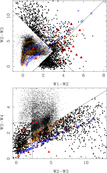
Figure 1: [W2–W3]$-$[W1–W2] and [W3–W4]$-$[W2–W3] CCDs. Red triangles are the sources from the template sample in Tab. 1. Small black triangles are selected sources (see main text). Small dots are non-selected sources; to avoid cluttering stricter SN criteria were applied for them to be plotted (see main text). Other symbols indicate sequences of increasing MLRs (see main text). Blue colours represent C-star models while orange colours represent O-star models for ($T_{\rm eff},T_{\rm inn}$) combinations of (2600, 1000), (3300, 800), and (4000, 400 K) in diamonds, five-pointed stars, and open plus signs, respectively.

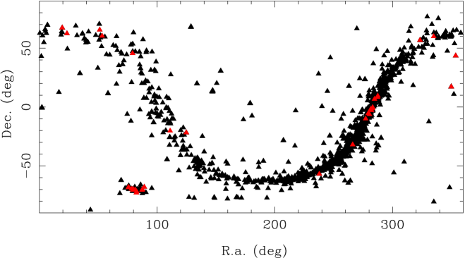
Figure 2: Distribution on the sky of the sample. Symbols are as in Fig. 1

3 Time series data and analysis

3.1 WISE

From the AllWISE multi-epoch photometry table and the NEOWISE-R single exposure source table all entries within 1″ of the AllWISE coordinates were downloaded in the W1 and W2 filters with the additional constraint that the error bars on the magnitudes were $<0.25$ mag and applying the flags saa_sep $>5$ and moon_masked $=0$ (e.g. Uchiyama & Ichikawa 2019). No other flags were applied (see Sect. 6.1).

At the bright end the WISE and NEOWISE data suffer from saturation that influences the photometry, and a correction was applied. Table 2 in Sect. II.1.c.iv.a of the NEOWISE Explanatory Supplement contains correction tables in the W1 and W2 filters for all phases of the mission. The corrections are negligible to small at W1 and W2 $\sim 7-8$ mag and reach almost 1.5 mag in W2 in NEOWISE-R. For stars brighter than the brightest entry in the tables the corresponding correction was kept without attempting any extrapolation. The Explanatory Supplement furthermore states that even with a correction, no useful information is available for sources brighter than W1 $\stackrel{{\scriptstyle<}}{{\sim}}$ 2 and W2 $\stackrel{{\scriptstyle<}}{{\sim}}$ 0 mag.

3.2 SAGE-VAR

For stars in the direction of the MCs the WISE W1 and W2 data were combined with IRAC 3.6 $\mu$m and IRAC 4.5 $\mu$m data, respectively, from the SAGE-VAR survey (Riebel et al., 2015) that adds four epochs from the warm SST mission at 3.6 and 4.5 $\mu$m for portions of the LMC and SMC. The filters of the IRAC 3.6 and 4.5 bands are similar but not identical to the WISE W1 and W2 filters and the transformation from Sloan et al. (2016) was used to bring the IRAC photometry to the WISE system.

3.3 Other time series data

As will be discussed below in detail, the literature was searched for known periods of the stars in the sample. However, next to quoting these periods, it turned out useful or even necessary to refit the original data in many cases for several reasons. In some cases the period in the literature seemed inconsistent with that expected for an LPV or inconsistent with that derived from the WISE data. In cases with multiple periods available from the literature these were sometimes inconsistent with each other. Also in the case of no or insufficient WISE data it seemed valuable to provide a pulsation period based on other data to the community. The major sources of additional time series photometry are described below.

The All-Sky Automated Survey for SuperNovae (ASAS-SN) (Shappee et al., 2014; Kochanek et al., 2017; Jayasinghe et al., 2018) identified 666 502 variables. From the survey website the basic data of these variables was downloaded which included the coordinates and the pulsation period. A search radius of 2″ was used to correlate it with the target list. In case the LC was refitted the $V$-band data were retrieved from this website as well.

The Asteroid Terrestrial-impact Last Alert System (ATLAS) (Tonry et al., 2018) published data on over 4.3 million candidate variable objects (Heinze et al., 2018). This dataset is available through the VizieR database and it was correlated with the target list using a search radius of 2″. The ATLAS team derived periods in several different ways and two are quoted, called fp-LSper (’original period from fourierperiod’s Lomb-Scargle periodogram’) and fp-lngfitper (’final master period from the long-period Fourier fit’). The original data were retrieved via a website following the instructions in Appendix B in Heinze et al. (2018). ATLAS observed in two bands and the redder one (the $o$-band peaking at 0.68 $\mu$m) is used to refit the LC.

Data from the Zwicky Transient Facility (ZTF) (Masci et al., 2019; Bellm et al., 2019) was downloaded following the suggestions on their website. This involved user-customised scripts using wget and a query to select the data. For the sources in the target list data is available in the Sloan $g$- and $r$-filters, and the redder one was used to refit the LC.

The VISTA Variables in the Vía Láctea (VVV) ESO Public Survey (Minniti et al., 2010) has been mapping the NIR variability in the $K_{\rm s}$-band of the Milky Way Bulge and the adjacent southern disk. Recently, Ferreira Lopes et al. (2020) published the VVV Infrared Variability Catalogue (VIVA-I) containing data on almost 45 million variable star candidates. The catalogue contains periods based on five different methods, and also a ’best period’, bestPeriod. From the VISTA Science Archive (VSA) the basic data of the 6.7 million sources in VIVA-I with a bestPeriod $>$ 0.5 days were downloaded, which was then cross-matched with the target sample using a search radius of 3″. In case the LC was refitted, the timeseries data were downloaded from a website using a dedicated query

ΩSELECT #upload.*, #proxtab.distance, d.RA, d.Dec,Ωd.filterID, d.mjd, d.aperMag3, d.aperMag3err,Ωd.ppErrBits FROM #upload leftΩouter join #proxtab on #upload.upload_id=upidΩleft outer join vvvDetection as d onΩd.objID=archiveID left outer join multiframe onΩmultiframe.multiframeId=d.multiframeID where frametypeΩlike ’tilestack’ order by upload_idΩ\end{verbatim}Ω

to obtain the publically available data.

The analysis of 3.6 years of data from the Diffuse Infrared Background Experiment (DIRBE) provided a list 597 (candidate) variables (Price et al., 2010). The data are available through VizieR and this includes coordinates, mean magnitudes and errors, amplitudes, and periods in four photometric bands. A pairing radius of 8″ was used. The VizieR table also includes a link to the time series data, which is used when the DIRBE data are refitted. In those cases the data at 4.9 $\mu$m was used as they are typically the brightest for the sources in the target list.

Data from other surveys has been analysed for a handful of sources, namely the Optical Monitoring Camera (OMC) data on board INTEGRAL (Alfonso-Garzón et al. 2012; one source), from the Catalina Sky Survey (CSS; Drake et al. 2009; three sources), the Bochum Galactic Disk Survey (GDS; Hackstein et al. 2015; two sources), and $K$-band photometry from Kerschbaum et al. (2006) with photometry from the literature being added (two sources). In addition, VMC $K$-band data from Groenewegen et al. (2020) were refitted with an improved initial period from the present work.

3.4 Period analysis and LC modelling

The automatic analysis of the LCs was carried out with the Fortran codes available in numerical recipes (Press et al., 1992) as described in Appendix A of Groenewegen (2004) and modified to analyse the VMC $K$-band data as described in Groenewegen et al. (2020). The Fourier analysis was done using the subroutine fasper. However, as a cross-check, most of the stars in the sample were analysed manually with the code Period04 (Lenz & Breger, 2005) as well. After an initial guess for the period was determined (either through the automatic routine, a period found in the literature, or from the manual fitting of the LC), a function of the form

$$m(t)=m_{0}+A\sin(2\pi\;t\;e^{f})+B\cos(2\pi\;t\;e^{f})$$ (1)

was fitted to the LC using the weighted linear least-squares fitting routine mrqmin. This results in the parameters listed in Tables LABEL:WISEREALPer, LABEL:noWISEPerbutREAL, and LABEL:WISEPernotREAL, namely mean magnitudes ($m_{0}$), periods ($\exp(-f)$), and amplitudes ($\sqrt{A^{2}+B^{2}}$) with their associated uncertainties. Equation 1 implies that the LC can be described by a single period. It is well known that the LCs of LPVs are not strictly single-periodic (as many of the fitted LCs show). However with the limited number of data points available one is in general not able to comment on the presence of more than one period.

A comparison of the LC with the fit sometimes suggested that alternative periods may be possible as well. These cases were inspected by the manual fitting of the LC using Period04, and alternative periods (denoted Palt) are sometimes indicated in the comments for Tables LABEL:WISEREALPer, LABEL:noWISEPerbutREAL, and LABEL:WISEPernotREAL. The tables also include the reduced $\chi^{2}$, defined as $\chi_{\rm r}^{2}=\sum_{\rm i}\left(((m_{\rm i}-o_{\rm i})/\sigma_{\rm o_{\rm i}})^{2}\right)/(N-N_{\rm p}),$ with $m$, $o$ and $\sigma_{\rm o}$ indicating the model magnitude, the observed magnitude, and the error, respectively, $N$ is the number of data points, and $N_{\rm p}$ = 1 or 4, depending on whether Eq. 1 is fitted without or with the period.

The Fourier analysis and the LC modelling were done on the W1 and W2 data separately. If the total time span of the data is less than 400 days, or the total number of data points is less than eight, the LC fitting process was terminated. This resulted in cases where only one LC was generated and these cases were inspected more closely. In most cases ($\sim 100$ stars) the data refer to a fake source in the AllWISE catalogue (see Sect. 6.1) and that source was removed from the fitting all together; in $\sim 15$ cases, the fit seemed reliable and in those cases the fitting process was carried out in the other filter using the available data, even if there were fewer than eight data points covering a shorter time span.

4 Literature data

To characterise the sources better, the target list was correlated with other databases. From the SIMBAD database, some common names and the object type were retrieved using a search radius of 3″.

Real sources that were detected in the W1 and W2 filters are expected to have been detected in other IR bands as well. To verify that, the target list was correlated with the following photometric catalogues which are all available through VizieR: 2MASS (Cutri et al., 2003) using a search radius of 1.0″; the Akari/IRC MIR all-sky survey (Ishihara et al., 2010a) using a search radius of 3.0″; the Midcourse Space Experiment (MSX) (Egan et al., 2003a) using a search radius of 5.0″; the Herschel infrared Galactic Plane Survey (Hi-GAL) 70 $\mu$m catalogue (Molinari et al., 2016), using a search radius of 4.5″; the Galactic Legacy Infrared Midplane Survey Extraordinaire (GLIMPSE) (Benjamin et al., 2003; Spitzer Science, 2009) using a search radius of 3.0″, and the MIPSGAL survey at 24 $\mu$m (Gutermuth & Heyer, 2015a) using a search radius of 2.0″. The first three surveys are all-sky, while the latter three are surveys mainly of the galactic plane.

Figure 2 shows that many sources are located in the galactic plane which has been surveyed extensively for OH maser emission. A double-peaked OH profile is a characteristic of evolved O-stars. The target list was correlated with the OH database of Engels & Bunzel (2015) using a search radius of 3.5″. OH maser sources in the MCs (Goldman et al., 2017, 2018) were also considered. The target list is also correlated with the classification of over 11 000 sources from IRAS LRS spectra (Kwok et al., 1997) that contains information on the dust species and continuum shape in the 8–23 $\mu$m region using a search radius of 12″, and with the compilation of spectral types (Skiff, 2014) using a search radius of 3.2″.

Finally, the target list was correlated with a number of catalogues containing extra galactic sources. There are no matches with the catalogues of ‘Quasars and Active Galactic Nuclei’ (13th ed., Véron-Cetty & Véron 2010), the ‘Large Quasar Astrometric Catalogue 4’ (Gattano et al., 2018), and the ‘SDSS quasar catalogue’ (DR16, Lyke et al. 2020). There are two matches in ‘The Million Quasars’ catalogue (version 7.2, April 2021; Flesch 2015), that lists a source at Ra= 286.187653, Dec= +48.885826 as having a 91% probability of being a QSO with a redshift of 0.700, and at Ra= 80.513848, Dec= -68.322622 as having a 69% probability of being a QSO with a redshift of 0.900.

There are more matches in catalogues listing AGN and QSO candidates, such as the ‘Gaia DR2 quasar and galaxy classification’ (Bailer-Jones et al. 2019, 60 matches), the ’QSO candidates catalogue with APOP and ALLWISE’ (Guo et al. 2018, 3 matches), and the ‘The WISE AGN candidates catalogues’ (the R90 90% reliability catalogue, Assef et al. 2018, 2 matches). The recent Gaia EDR3 list of AGN and QSOs (Gaia Collaboration et al., 2021a, b) contains 3 matches within 1 arcsec. These matches are listed in Tables LABEL:WISEREALSam, LABEL:noWISESambutREAL, and LABEL:WISESamnotREAL from which it is clear that many are actually stellar sources. For example, of the 60 candidate QSOs in Bailer-Jones et al. (2019) 39 show LPV-like pulsations (see Sect. 6.4). The target list was also correlated with the catalogue of Solarz et al. (2017). They used a novel approach (one-class support vector machines, OCSVM) to identify anomalous patterns in AllWISE colours. Their method allowed them to detect anomalies (e.g. objects with spurious photometry), and also real sources such as a sample of heavily reddened AGN/quasar candidates.

5 Results

The results of the literature search and the period analysis are compiled in Tables LABEL:WISEREALSam-LABEL:WISEPernotREAL. There is a table listing the results of the literature search and a table listing the results of the period analysis for three classes of objects: 1224 bona fide stellar sources with a period analysis based on WISE data (Tables LABEL:WISEREALSam, LABEL:WISEREALPer); 118 bona fide stellar sources without sufficient WISE data for the LC analysis in both filters, but possibly with a period from the literature or analysis of literature data (Tables LABEL:noWISESambutREAL, LABEL:noWISEPerbutREAL); and 650 other sources that may contain a few extra galactic objects, but most are not bona fide sources (Tables LABEL:WISESamnotREAL, LABEL:WISEPernotREAL).

The distinction between the bona fide stellar sources and those that (very likely) are not is based on the number of associations with a SIMBAD object and the other external catalogues mentioned in Sect. 4, an inspection of the LC, and the result of the LC fitting. Signatures of a fake source are no, or only one association with an external catalogue (often close to the limit of the search radius used), and a LC with a few points. They are further discussed in Sect. 6.1.

Tables LABEL:WISEREALSam, LABEL:noWISESambutREAL, and LABEL:WISESamnotREAL contain the results of the literature search and they include the distance to the closest SIMBAD object and the other photometric catalogues discussed in Sect. 4. This also includes the blue and red velocity of any OH maser emission, the IRAS LRS classification, and the spectral type. Tables LABEL:WISEREALPer, LABEL:noWISEPerbutREAL, and LABEL:WISEPernotREAL contain the periods quoted in the literature, the periods derived from fitting literature data, and the results of fitting the WISE data (period with error, amplitude with error, mean magnitude with error, and the reduced $\chi^{2}$ in the W1 and W2 filters). Examples of the lightcurve and the fits are shown for both the WISE data (Fig. 8) and the other fitted data from the literature (Figs. 9-13). The complete set of fitted LCs is available at https://doi.org/10.5281/zenodo.5825878. Figures 14–18 show the LCs for the datasets with a limited number of matches that can fit in a single figure.

6 Discussion

6.1 AllWISE sources that are very likely not real

In inspecting the coordinates of the mostly fake objects (Table LABEL:WISESamnotREAL) it is striking to observe that they can be very similar, and in fact many are related to very bright objects (hereafter, ‘clones’). The most conspicuous example are the clones of CW Leo. CW Leo is located at (Ra, Dec)= (146.989193, $+13.278768$) and it is not present in the AllWISE catalogue. In the target list, there are 42 sources located up to 17′ from this position not associated with any other known source. Other well-known IR bright sources have clones, including AFGL 3068 (Ra, Dec= 349.802533, $+17.192628$, W1= 4.7 mag, W2 is unreliable; 16 sources up to 9′), VY CMa (Ra, Dec= 110.7430362, $-25.7675659$, W1 $\sim$ 1.7 mag and W2 $\sim$ 3.4 mag but both are unreliable; nine sources up to 10′), or IRC +10 420 (Ra, Dec= 291.700408, $+11.354634$, not in AllWISE; seven sources up to 9′). For a slightly fainter source such as IRAS 08171$-2134$ (Ra, Dec= 124.8263077, $-21.737400$, W1=7.3 mag and W2=3.8 mag), the number is reduced to three sources up to 1.2′ distance.

Some of these clones have LCs that are periodic (see Fig. 3) with periods in agreement with the literature values. These are CW Leo $P=643\pm 1.4$ d (the weighted mean of the periods obtained in the W1 and W2 bands, cf. Table LABEL:WISEPernotREAL) compared to $P=639\pm 4$ (e.g. Groenewegen et al. 2012 and references therein), IRAS 15194-5115 $P=565\pm 2.3$ d compared to $P=580$ (Le Bertre, 1992) and $P=576$ (Whitelock et al., 2006), IRC +20 326 $P=549\pm 3.6$ d compared to $P=540$ (Uttenthaler et al., 2019), AFGL 3116 $P=630\pm 3.3$ d compared to $P=620$ (Jones et al., 1990) or $P=599$ (Drake et al., 2014), and AFGL 2135 $P=619\pm 13$ d compared to $P=655$ (Whitelock et al., 2006).

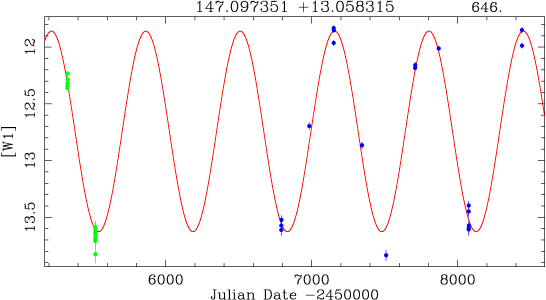
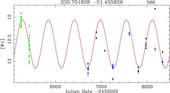
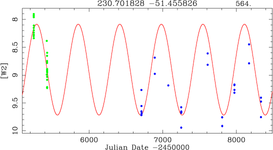
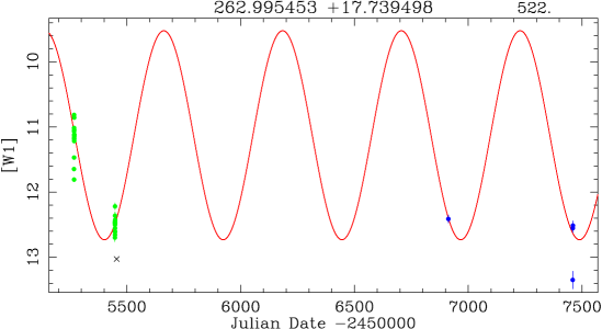
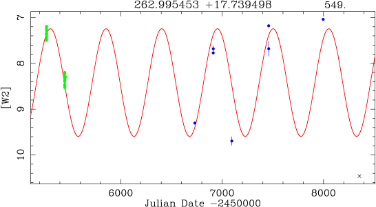
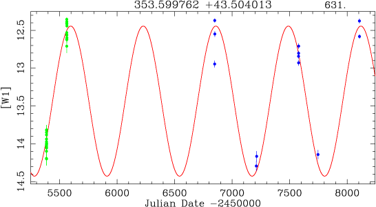
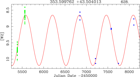
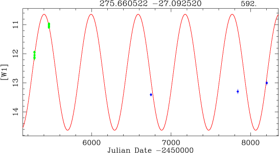
Figure 3: Examples of LC fits (W1 in the left-hand panel and W2 in the right-hand panel) to clones of CW Leo (Ra= 147.097351), IRAS 15194-5115 (Ra= 230.701828), IRC +20 326 (Ra= 262.995453), AFGL 3116 (Ra= 353.599762), and AFGL 2135 (Ra= 275.660522). The identifier is listed on top of each panel, with the period to the right.

The number of fake sources is almost one-third of the sample and one may wonder if these could have been filtered out using flags available in the AllWISE catalogue. Both Chen et al. (2018) and Uchiyama & Ichikawa (2019) used additional selection criteria, for example on the photometric quality (ph_qual), contamination and confusion flag (cc_flags), variability flag (var_flag), fraction of saturated pixels (w?sat), or poor PSF profile fitting (w?rchi2), where ‘?’ stands for ‘1’ or ‘2’ depending on the filter.

Among the fake sources 86% have a cc_flag in the W1 and W2 filter which is not equal to ’00’, but so do 77% of the bona fide sources. The fake sources also do not necessarily have poor photometric quality flags (77% in fact have a ph_flag in the W1 and W2 filter of ‘AA’). Other flags were inspected, but in conclusion, many bona fide sources with good quality data would be eliminated by applying stricter selection criteria, although this implies including a significant number of fake sources.

6.2 Sources in the VVV survey

Of the 122 sources analysed by Ferreira Lopes et al. (2020), 51 are listed with a period of 1 day (when rounded to one digit) and another ten with periods below 10 days. Out of the remaining 61, only nine periods agree to within 10% with the periods derived here; while in 32 cases, the difference in period is more than a factor of two, and up to a factor of ten. The reason for this large discrepancy is very likely related to the frequency range that was explored in Ferreira Lopes et al. (2020), which is namely larger than $\frac{2}{T}$ $d^{-1}$, with $T$ being the time span (see Sect. 4.2 of that paper). This time span is not explicitly given and likely varies from source to source, but it probably leads to a lower frequency limit that is too large. In fact, an earlier paper by the VVV team (Contreras Peña et al., 2017) that searched for high-amplitude infrared variable stars lists different periods for a number of stars (they do not state what frequency range they searched). Out of the ten sources in the sample with periods in Contreras Peña et al. (2017), nine have a period from WISE data of which seven agree to within 10% and all nine to within 20%. The periods listed in Ferreira Lopes et al. (2020) for those stars are all incorrect (three have a period of one day or periods are too small by factors of 1.7 to 3.2).

As an additional check, for a sample of 49 stars the $K$-band data from the VVV sources were reanalysed using the publically available data. For 42, the periods derived in this way agreed to within 10% with the period from the WISE data. All the revised periods and LCs are available in the Appendices, as explained at the end of Section 5.

6.3 Non-variable OHIR stars

In a recent paper, Kamizuka et al. (2020) investigated the NIR brightening of non-variable OH/IR stars. The OH maser emission of OH/IR stars on the AGB is expected to follow the pulsation period of the underlying star, see Sect. 2.2. However, non-variable OH/IR stars are known to exist (Herman & Habing, 1985) and this is expected to happen in the transition from the AGB to the P-AGB phase when large-amplitude pulsations stop.

Kamizuka et al. (2020) selected 16 stars from the sample in Herman & Habing (1985), which had the smallest variability amplitudes in their OH/IR maser emission. They established NIR multi-epoch data for six objects, based on archival data from 2MASS (Cutri et al., 2003), UKIDSS (Lucas et al., 2008), and data taken with the Okayama Astrophysical Observatory Wide Field Camera (OAOWFC; Yanagisawa et al. 2019). For all six stars, they derived a brightening in the $K$-band in the range $0.01-0.13$ mag/year over a 20 year period for five objects.

Of the 16 objects studied in Kamizuka et al. (2020), four are in the WISE sample: OH $17.7-2.0$ (ra=277.627928) and OH $31.0+0.0$ (ra=281.921407) that are not among the six for which Kamizuka et al. (2020) determined a NIR brightening, and OH $31.0-0.2$ (ra=282.179217) and OH $37.1$$-0.8$ (ra=285.526137) for which they determined a brightening of 2.04 mag over 2250 d (0.33 mag/yr) and 0.35 mag over 2170 d (0.06 mag/yr), respectively, however based on only two data points in both cases.

The W1 and W2 LCs for these four objects are shown in the top four panels of Fig. 4. We note that OH $17.7-2.0$ is becoming fainter by $\sim 0.7$ (W1) and $\sim 0.4$ (W2) mag over $\sim 3200$ d ($\sim 0.05-0.08$ mag/year). For OH $31.0+0.0$, the situation is less clear in W1, but in the W2 filter there is a faintening by $\sim 0.4$ mag. Also, OH $31.0-0.2$ is not clearly brightening or faintening. The formal LC fitting gives very long periods, which must be taken with caution as the time span of the WISE observations covers less than half of the putative pulsation period. The two $K$-band data points considered by Kamizuka et al. (2020) were taken at epochs 2453536 and 2455787. The WISE LCs do show a brightening between 2455200 and the last $K$-band epoch. Furthermore, OH $37.1-0.8$ shows a marginal brightening of order 0.2 mag over 8.7 years in both filters.

Along similar lines, Lewis (2002) observed the OH maser emission of 328 stars after 12 years again to find four with undetectable emission at re-observation, and one in ’terminal decline’. One of these five stars is in the sample (IRAS 18455+0448, ra=282.009613) and its WISE LC is shown in the bottom panels of Fig. 4. Its WISE emission is consistent with no variation.

To investigate this more systematically, the light curves of all stars in the sample were inspected that either have a SIMBAD classification as an OH/IR star (Col. 5 in Tables LABEL:WISEREALSam, LABEL:noWISESambutREAL, LABEL:WISESamnotREAL) or an entry in the database of Engels & Bunzel (2015) (Col. 12/13 in those tables). All stars with a period from analysis of the WISE data, a period from the literature or from refitting literature data, as well as stars not detected in OH and classified different from an O-rich star, were removed. Twenty new candidate non-variable OH/IR stars were identified. They are labelled with ‘nvoh’ in column 20 in Tables LABEL:WISEREALPer and LABEL:noWISEPerbutREAL. The five objects in the sample previously identified in the literature are labelled with ‘NVOH’ in those tables.

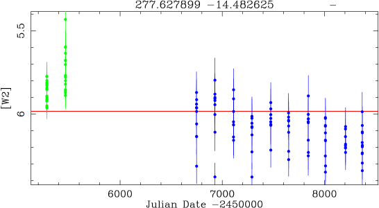
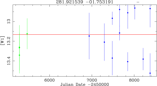
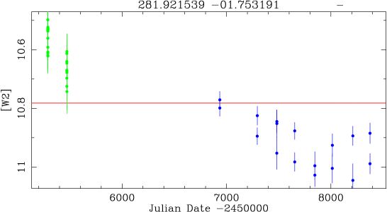
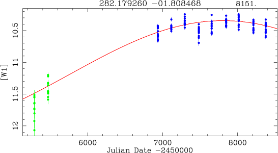
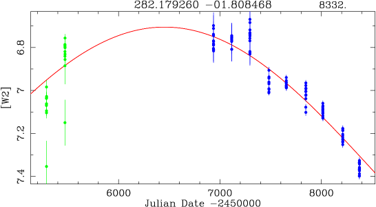
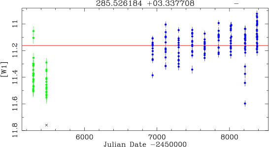
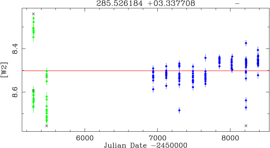
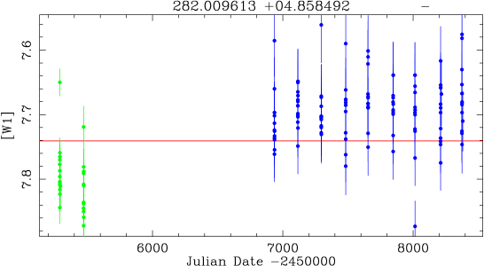
Figure 4: WISE LCs of non-variable OH/IR stars in the sample.

6.4 Selecting LPVs

The selection of (candidate) LPVs from the WISE data is based on the amplitude. The geometric mean of the amplitude in the W1 and W2 filters (AmpW) and the errors therein ($\sigma_{\rm AmpW}$) were calculated. LPV candidates are those with AmpW $>0.2$ mag, AmpW/$\sigma_{\rm AmpW}>2.5$ and a SN $>6$ in the amplitude detection in either the W1 or W2 filter. One well-known LPV (AFGL 3068, Ra= 349.802533) was added manually to this list. The cut in amplitude is chosen to correspond roughly with typical cut-off values of about 0.45 mag used in the $I$-band and of about 0.2 mag in the and $K$-band. The cuts on the SN ratio were determined empirically by visually inspecting the LCs and fits to the LCs of stars selected in this way, and those that are not. In this way 752, LPVs were selected, of which 356 appear to be newly classified as such. They are marked ‘LPV’ in Tables LABEL:WISEREALSam and LABEL:noWISESambutREAL. However, there always remain some borderline cases where the LC of an LPV candidate appears noisy, and only higher precision photometry over a sufficiently long time span may resolve the variable nature of some sources. One hundred fourty-five sources have periods longer than 1000 days of which 109 are new (13 had previously quoted periods below 1000, typically 160-700 days), which is a significant increase in the 16 template sources in Table 1 from Menzies et al. (2019). The referee directed us to the paper by Chen et al. (2020) which analysed and classified a large number of variable stars based on ZTF data. A comparison with the periods derived in the present paper based on WISE data and ZTF data is presented in Appendix E.

The list of non-LPV candidates selected in this way (the complementary sample) contains interesting sources, some of which are periodic, but with a smaller amplitude, or where a good LC fit is obtained in one filter only, or they show peculiar LCs. These sources are marked ‘PER’ in Tables LABEL:WISEREALPer and LABEL:noWISEPerbutREAL. They include known OH/IR stars, also sometimes with a period derived from the literature, but with poor WISE data in one filter, in addition to Sakurai’s object (see Evans et al. 2020 for a detailed discussion on its $K$ and WISE LC). Examples of LCs for such sources are displayed in Fig. 19.

6.5 EROs and the mass return to the ISM

As the (rare) C-rich stars with the highest MLRs dominate the mass return by AGB stars to the ISM (see references in the introduction) it is of interest to identify new objects in this class, both in the Galaxy and the MCs. The template sample in Table 1 of EROs is based on the shape of the spectrum in the MIR (a red flat continuum or the SiC feature in absorption), but spectral data are generally not available, only photometric data are. Based on the colours in Table 1, the spectral energy distributions (SEDs) of the 316 objects with W2$-$W3 $>$ 3.0 mag were constructed using data in the literature. For a subset of 141 stars, MIR spectra were available. The SEDs were fitted with the dust radiative transfer code more of DUSTY (MoD, Groenewegen 2012), which is an extension of the radiative transfer code DUSTY (Ivezić et al., 1999), allowing the derivation of luminosities and MLRs; the details are given in Appendix C.

Distances to the galactic sources were derived as follows. Based on the C-rich objects in the MCs the following period-luminosity ($PL$) relation was derived (see details in Appendix C and shown in Fig. 20),

$$M_{\rm bol}=-5.07\cdot(\log P-2.8)-4.47\leavevmode\nobreak\ {\rm mag},$$ (2)

based on 31 objects and with an rms of 0.31 mag. This $PL$ relation was then applied to the Galactic objects for which a period was available, O- and C-rich alike. The $PL$ relation was derived using stars with periods up to $\log P\approx 3.1$ (about 1260 days), while the longest period for which it has been applied has a period of about 2600 days ($\log P\approx 3.4$). For C-stars without a period the median luminosity of 7100 L_⊙ of the MCs objects with a period was used; for the O-rich objects without a period an arbitrary distance of 2.0 kpc was adopted. Interstellar (IS) reddening was included (see Appendix C). That notion that the $PL$ relation derived for ERO C-stars in the MCs would hold for Galactic C-stars, and for O-stars, is an assumption made here. Data for less reddened and shorter period ($P\raisebox{-3.1298pt}{$\stackrel{{\scriptstyle<}}{{\sim}}$}400$ d) Miras are consistent with the premise that any differences are small (Whitelock et al., 2008). We note that, to first order, ignoring the dependence of the reddening on distance, $L\sim d^{2}$ and $\dot{M}$$\sim d$ if the reader prefers another distance.

Based on the MIR spectra and the fitting of the SED, the sample was divided into 197 C-rich and 119 O-rich sources. Of the C-rich sources, 18 belong to the sample of Galactic and LMC template sources of EROs (and are labelled ERO in Tables LABEL:WISEREALSam and LABEL:noWISESambutREAL), 65 sources (including eight in the LMC) are EROs with MIR spectra (and are labelled eroS in these Tables), 110 sources (including two in the direction of the SMC, and 26 in the direction of the LMC) are candidate EROs based on the fitting of the SEDs (and are labelled eroP in these Tables), and the remaining four are classified as C-rich non-ERO sources (and are labelled sedC in these Tables) The O-rich sources appear to be a mixture of O-rich AGB and P-AGB stars, Hii regions, planetary nebulae and YSOs (and are labelled sedO in these Tables).

Table 2 show the results for the C-stars and Table 9 for the O-stars. Only the first entries are shown, and the full tables are available at the CDS. Displayed are the adopted distance and reddening and the results of fitting the SEDs. The last column shows the total MLR, which assumes spherical symmetry of the CSE, a dust-to-gas (DTG) ratio of 0.005, and a CSE expansion velocity of 10 km s^-1 for every star.

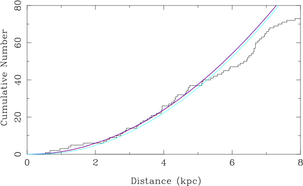
Figure 5: Cumulative number distribution of ERO (candidates) versus distance. The right-hand panel is a zoom, and it shows model predictions for combinations of local space density and vertical scale height of 1.6 kpc^-3, 150 pc (dark blue); 0.8 kpc^-3, 300 pc (red); and 0.30 kpc^-3, 800 pc (light blue), respectively.

Figure 5 shows the cumulative number distributions of ERO (candidates) versus distance up to 30 kpc on the left, and up to 8 kpc on the right. When the number density of stars is assumed to depend exponentially on the height above the Galactic plane the number of stars within a certain radius can be calculated analytically, see Eq. 19 in Groenewegen et al. (1992), while Eq. 20 in that paper can be used to determine the scale height. The right-hand panel of Figure 5 shows some models for different scale heights ($H$) and local space densities ($\rho_{0}$). The number of objects scales to first order with ($H\cdot\rho_{0}$) and the three models that show a very similar behaviour all have $H\cdot\rho_{0}=0.24$ kpc kpc^-3. Groenewegen et al. (1992). based on a very small number of EROs derived $H$ = 195 $\pm$ 20 pc, and $H\cdot\rho_{0}=0.23-0.27$ kpc kpc^-3.

The predicted number of stars versus distance suggests that the sample of EROs may be complete up to 5 kpc. There are 36 stars in a cylinder around the Sun with this distance with a total estimated MLR of 4.1 $\cdot 10^{-4}$ M_⊙ yr^-1 (or 5.2 $\cdot 10^{-6}$ M_⊙ yr^-1/kpc²) and an estimated scale height of 180 pc. The average MLR is this sample is 1.1 $\cdot 10^{-5}$ M_⊙ yr^-1. As the DTG ratio is an assumed quantity (1/200), a more certain number is the dust-production rate (DPR) which is 2.0 $\cdot 10^{-6}$ M_⊙ yr^-1 (or 2.6 $\cdot 10^{-8}$ M_⊙ yr^-1/kpc²). To estimate an uncertainty on these numbers, Monte Carlo calculations were performed generating samples with other distances and MLRs, assuming Gaussian distributions with a width of 0.3 mag in $M_{\rm bol}$ (which leads to a change in distance and in MLR), a condensation temperature taking the estimated error from Table 2 (with a minimum of 50 K), and an optical depth taking the estimated error from Table 2. The 2.7%, 97.3%, and 50% percentiles (corresponding to $\pm$2$\sigma$ in a Gaussian distribution and the median) indicate a number of stars of 37 (33-41; 0.4-0.5 kpc^-2), a cumulative MLR of 4.0 (3.3-6.0 $\cdot 10^{-4}$ M_⊙ yr^-1), and a $H=190$ (156-224 pc). Changing the limiting distance to 3 kpc has some impact on the estimated DPR per unit surface area from 2.6 (2.1-3.8 $\cdot 10^{-8}$ M_⊙ yr^-1/kpc²) to 2.3 (1.7-3.0 $\cdot 10^{-8}$ M_⊙ yr^-1/kpc²). The number of stars is reduced to the range 13 to 18 with a median of 16. All (dust) MLRs quoted above are based on an average expansion velocity of 10 km s^-1. If this were 15 km s^-1 (as assumed in e.g. Jura & Kleinmann 1989), all MLRs would increase by a factor of 1.5.

The cumulative mass-loss return of the 45 ERO sources in the LMC is 1.0 $\cdot 10^{-3}$ M_⊙ yr^-1  (or 5.0 $\cdot 10^{-6}$ M_⊙ yr^-1 in dust). Thirty-three were modelled by Nanni et al. (2019), finding a total MLR of 7.8 $\cdot 10^{-3}$ M_⊙ yr^-1 (and 3.3 $\cdot 10^{-6}$ M_⊙ yr^-1 in dust) and implying an average gas-to-dust ratio of 240. Here we find 7.3 $\cdot 10^{-3}$ M_⊙ yr^-1  (or 3.7 $\cdot 10^{-6}$ M_⊙ yr^-1 in dust) for that sub-sample, which is in good agreement. What is interesting and in highlighting, again, the importance of the EROs is the impact of the only 12 stars not included in the study by Nanni et al. (2019). The total dust return by C-stars for the entire LMC is 16.0 $\cdot 10^{-6}$ M_⊙ yr^-1 (J1000 models; Nanni et al. 2019) from 8239 stars, of which 82% (13.1 $\cdot 10^{-6}$ M_⊙ yr^-1) are by the 16% (1332) classified as X-stars. The sub-sample of 33 stars (0.4%) already contributes 21% to the total dust return. Adding the other 12 stars (0.15%) augments the total dust return by 8% to about 17.3 $\cdot 10^{-6}$ M_⊙ yr^-1.

Table 2: Fit results of the C-star sample (first entries)

RA	Dec	Period	$d$	$A_{\rm V}$	$T_{\rm eff}$	$L$	$\tau_{0.5}$	$T_{\rm c}$	f	$p$	f	$\dot{M}$
(deg)	(deg)	(days)	(kpc)	(mag)	(K)	(L⊙)		(K)				(M⊙ yr-1)
19.463942	67.231445	1047	2.74	3.73	3300	13214 $\pm$ 75	170 $\pm$ 1.5	1000 $\pm$ 0	0	2.0 $\pm$ 0.0	0	0.262E-04
349.802521	17.192619	746	0.77	0.23	2700	6661 $\pm$ 108	95 $\pm$ 0.9	1000 $\pm$ 0	0	2.0 $\pm$ 0.0	0	0.893E-05
353.599762	43.504013	629	0.67	0.36	2500	4729 $\pm$ 66	15 $\pm$ 0.2	716 $\pm$ 7	1	2.0 $\pm$ 0.0	0	0.206E-05
124.826309	-21.737400	939	2.80	0.20	3300	10621 $\pm$ 219	136 $\pm$ 3.9	1000 $\pm$ 0	0	2.0 $\pm$ 0.0	0	0.167E-04
287.486908	9.447611	1071	2.32	5.45	2800	13014 $\pm$ 341	99 $\pm$ 1.6	1201 $\pm$ 0	0	2.0 $\pm$ 0.0	0	0.977E-05
237.773834	-56.890007	951	2.51	1.54	2500	10605 $\pm$ 262	57 $\pm$ 0.5	655 $\pm$ 17	1	2.0 $\pm$ 0.0	0	0.149E-04
323.345001	56.743065	930	2.03	2.54	2600	10334 $\pm$ 187	109 $\pm$ 2.6	1000 $\pm$ 0	0	2.0 $\pm$ 0.0	0	0.122E-04
75.631233	-68.093285	1884	50.00	0.22	2700	7897 $\pm$ 44	251 $\pm$ 1.8	1000 $\pm$ 0	0	2.0 $\pm$ 0.0	0	0.304E-04
76.023376	-68.394501	-	50.00	0.22	3100	5992 $\pm$ 10	248 $\pm$ 0.9	1000 $\pm$ 0	0	2.0 $\pm$ 0.0	0	0.262E-04
79.548790	-70.507469	-	50.00	0.22	3200	9496 $\pm$ 18	273 $\pm$ 1.0	1000 $\pm$ 0	0	2.0 $\pm$ 0.0	0	0.330E-04
79.701599	-69.559563	-	50.00	0.22	3100	6935 $\pm$ 10	189 $\pm$ 0.6	1000 $\pm$ 0	0	2.0 $\pm$ 0.0	0	0.199E-04
81.419411	-70.140877	-	50.00	0.22	3000	4000 $\pm$ 10	205 $\pm$ 1.1	1000 $\pm$ 0	0	2.0 $\pm$ 0.0	0	0.167E-04
82.407959	-72.831322	678	50.00	0.22	2800	5498 $\pm$ 18	125 $\pm$ 0.7	1000 $\pm$ 0	0	2.0 $\pm$ 0.0	0	0.116E-04
87.608788	-69.934212	1110	50.00	0.22	2600	10351 $\pm$ 12	111 $\pm$ 3.8	743 $\pm$ 15	1	2.0 $\pm$ 0.0	0	0.245E-04
78.257469	-69.564110	-	50.00	0.22	2600	6381 $\pm$ 21	274 $\pm$ 1.4	1000 $\pm$ 0	0	2.0 $\pm$ 0.0	0	0.307E-04
82.684006	-71.716766	954	50.00	0.22	3600	8233 $\pm$ 29	46 $\pm$ 1.8	269 $\pm$ 5	1	2.0 $\pm$ 0.0	0	0.103E-03
87.249886	-70.556229	3434	50.00	0.22	3000	12280 $\pm$ 28	85 $\pm$ 1.4	283 $\pm$ 3	1	2.0 $\pm$ 0.0	0	0.182E-03
89.161446	-67.892776	1220	50.00	0.22	4000	20161 $\pm$ 136	74 $\pm$ 0.8	1000 $\pm$ 0	0	2.0 $\pm$ 0.0	0	0.121E-04
5.961981	62.636379	1065	4.98	2.21	2800	13619 $\pm$ 261	93 $\pm$ 2.3	1000 $\pm$ 0	0	2.0 $\pm$ 0.0	0	0.116E-04
38.251453	58.035065	827	2.33	1.69	2400	8209 $\pm$ 803	46 $\pm$ 1.5	642 $\pm$ 33	1	2.0 $\pm$ 0.0	0	0.119E-04
39.529259	54.587803	905	4.63	1.04	2400	9856 $\pm$ 223	75 $\pm$ 2.7	1000 $\pm$ 0	0	2.0 $\pm$ 0.0	0	0.770E-05
41.103512	55.187542	477	3.95	1.64	2400	2691 $\pm$ 78	78 $\pm$ 5.6	514 $\pm$ 32	1	2.0 $\pm$ 0.0	0	0.187E-04
47.976738	60.956123	1163	8.11	3.52	3300	16391 $\pm$ 266	68 $\pm$ 1.9	1000 $\pm$ 0	0	2.0 $\pm$ 0.0	0	0.899E-05
57.080860	44.701607	731	1.65	1.33	2400	6370 $\pm$ 104	27 $\pm$ 0.6	842 $\pm$ 19	1	2.0 $\pm$ 0.0	0	0.266E-05
72.919174	-68.792953	784	50.00	0.22	4000	5328 $\pm$ 15	80 $\pm$ 0.5	1000 $\pm$ 0	0	2.0 $\pm$ 0.0	0	0.729E-05
74.691780	-68.343849	777	50.00	0.22	5000	6900 $\pm$ 63	40 $\pm$ 1.5	736 $\pm$ 16	1	2.0 $\pm$ 0.0	0	0.859E-05
76.270149	-68.963379	938	50.00	0.22	3000	9645 $\pm$ 154	83 $\pm$ 2.0	1000 $\pm$ 0	0	2.0 $\pm$ 0.0	0	0.850E-05
76.646332	-70.280640	554	50.00	0.22	5000	8943 $\pm$ 92	22 $\pm$ 0.8	682 $\pm$ 15	1	2.0 $\pm$ 0.0	0	0.592E-05
78.003212	-70.540047	1182	50.00	0.22	4000	15047 $\pm$ 77	55 $\pm$ 0.5	1000 $\pm$ 0	0	2.0 $\pm$ 0.0	0	0.740E-05
82.525955	-70.511375	807	50.00	0.22	3200	9845 $\pm$ 115	64 $\pm$ 1.1	1200 $\pm$ 0	0	2.0 $\pm$ 0.0	0	0.474E-05
85.336433	-69.078796	895	50.00	0.22	2700	9363 $\pm$ 84	63 $\pm$ 2.7	764 $\pm$ 23	1	2.0 $\pm$ 0.0	0	0.108E-04
87.485626	-70.886604	1041	50.00	0.22	2600	17597 $\pm$ 264	27 $\pm$ 2.1	794 $\pm$ 26	1	2.0 $\pm$ 0.0	0	0.543E-05
91.000160	7.431088	696	1.28	0.83	2400	5818 $\pm$ 103	31 $\pm$ 0.5	775 $\pm$ 19	1	2.0 $\pm$ 0.0	0	0.353E-05
91.039764	47.795067	934	5.15	0.43	2400	10507 $\pm$ 225	86 $\pm$ 3.0	1000 $\pm$ 0	0	2.0 $\pm$ 0.0	0	0.935E-05
95.182762	-4.558214	1795	23.15	0.77	2700	39535 $\pm$ 1639	257 $\pm$ 11.1	1000 $\pm$ 0	0	2.0 $\pm$ 0.0	0	0.700E-04
99.256760	-1.450483	854	4.36	2.71	2400	8762 $\pm$ 243	42 $\pm$ 2.3	1000 $\pm$ 0	0	2.0 $\pm$ 0.0	0	0.371E-05

6.6 The nature of the EROs

Although the C-rich EROs are thought to be major contributors to the dust and mass return of AGB stars to the ISM the nature of these objects is not fully understood. Many are clearly pulsating with large amplitudes and are LPVs. They follow a well-defined $PL$ relation up to about 1260 days (see Fig. 20). These objects definitely show the characteristics of AGB evolution. However, there are also objects that are classified as EROs based on the SEDs and MIR spectra that show no clear evidence for pulsation or variability, or with different properties.

This was first recognised in Sloan et al. (2016) where it is remarked that some of the embedded sources are relatively non-variable and that some have relatively blue colours (compared to other embedded sources) at shorter wavelengths and that this can be interpreted as the central star revealing itself. They conclude that some deeply embedded stars may be evolving off of the AGB and/or they may have non-spherical dust geometries.

One of the parameters derived from the SED fitting is the temperature at the inner radius. In most cases, a standard value (800-1200 K, consistent with the condensation temperature of amorphous carbon dust) is sufficient to fit the data. However, for a non-negligible fraction of objects, a lower value has to be adopted, and this can be due to non-spherical dust geometries, or a spherical shell that expands, consistent with the drop in MLR when the AGB star evolves into the P-AGB phase. Of the 133 objects with a condensation temperature consistent with 800 K or more, 116 show a plausible pulsation period, and only 12% show no obvious variability or a period longer than 1300 days. For one-third of the sample (64 stars), a lower dust temperature at the inner radius is inferred of which 73% show no obvious variability or a period longer than 1300 days. This implies that lower temperatures at the inner radius are found for a non-negligible number of objects and that these show, on average, less pronounced variability.

However, one issue with the interpretation of some of these stars evolving from the AGB into the P-AGB phase is the timescale. To investigate this further the SEDs and MIR spectra were calculated for two objects under the assumption that the MLR drops abruptly to zero and that the CSE then expands at a velocity of 10 km s^-1. The results are shown in Fig. 6. The models in Fig. 6 were calculated for an effective temperatures typical for AGB stars (2600-2800 K). The P-AGB models of Miller Bertolami (2016) indicate that the effective temperature of stars with an initial mass of 2 and 3 M_⊙ is about 3800 K at an envelope mass of 0.01 M_⊙. Similar calculation were done for $T_{\rm eff}=3800$ K and are shown in Fig. 22. The differences are small. The change in effective temperature at that phase of the evolution is also small, 0.22-0.52 K/year. A first indication that the central star becomes slightly visible is present already after the order of 20-30 years. When the dynamical time increases the central star becomes increasingly visible, until after about 500 years one has the classical SED of a P-AGB star with a double-peaked SED. Important here is that the MIR bump remains bright and red, and so any selection of a sample based on MIR colours and magnitudes would be relatively insensitive to the expanding shell. One would therefore expect more objects in the sample of (candidate) EROs which show hints of a double-peaked SED, and this is not the case.

Recently Dell’Agli et al. (2021) propose that binary interaction mechanisms that involve common envelope evolution (CEE) could be a possible explanation, and that these stars could possibly hide binaries with orbital periods of the order of days. Their main argument is that single-star stellar evolution models combined with dust formation models could not produce the location of the EROs in certain colour-colour diagrams, and that this implies MLRs of 1-2 $\cdot 10^{-4}$ M_⊙ yr^-1 or larger. A binary scenario involving CEE might trigger the amount of dust to produce the observed colours. For the 11 stars in Table 1 in Dell’Agli et al. (2021), MLRs of (0.7-3.3) $\cdot 10^{-5}$ M_⊙ yr^-1 are found for nine in the present study, that is significantly lower than $10^{-4}$ M_⊙ yr^-1 (for our choice for the DTG ratio and expansion velocity). For SSID 125 (ra=82.684006) and SSID 190 (ra=87.249886), very large MLRs of 1.0 and 1.8 $\cdot 10^{-4}$ M_⊙ yr^-1 were indeed derived, respectively. The MLR in the latter source is the largest for all (candidate) EROs in the MCs, and only two show larger MLRs in our Galaxy, namely 2.1 $\cdot 10^{-4}$ M_⊙ yr^-1 (ra=283.812347), and 3.1 $\cdot 10^{-4}$ M_⊙ yr^-1 (ra=328.768372).

In the sample of EROs in the MCs that define the $PL$ relation, two objects were excluded as their periods (1884 and 3434 days but with large uncertainty) and luminosity did not match the relation. Similarly, among the Galactic ERO candidates, there are a few sources with (uncertain) periods in the range of 2000-5000 days where the $PL$ relation was not applied. The longest period for which it was applied was about 2600 days. For longer periods, the implied luminosity would no longer be compatible with the AGB ($L\raisebox{-3.1298pt}{$\stackrel{{\scriptstyle>}}{{\sim}}$}100\leavevmode\nobreak\ 000\leavevmode\nobreak\ \mbox{L${}_{\odot}$}$). For a few stars with shorter periods (1000-2000 days) located close to the Galactic plane, the $PL$ relation is also unlikely to be valid. The implied luminosities from the $PL$ relation are compatible with the AGB, but they lead to large distances ($\stackrel{{\scriptstyle>}}{{\sim}}$20 kpc) that imply large reddenings ($A_{\rm V}\raisebox{-3.1298pt}{$\stackrel{{\scriptstyle>}}{{\sim}}$}10$ mag) that are incompatible with the observed SEDs that show less extinction.

In summary, the nature of the EROs remain uncertain. Many show properties that are consistent with the properties expected for evolved AGB stars, but a significant fraction of them do not. The P-AGB channel may apply to some, but the time evolution of an expanding (spherical) shell would predict more objects with a classical double-peaked SED. The CEE channel is interesting, but it will be hard to prove the predicted binary period of the order of days. The derived MLRs are in general lower than predicted, although this depends on the assumed DTG ratio and expansion velocity, but in addition to the adopted MLR formalism in the stellar evolution models, which Dell’Agli et al. (2021) acknowledge might be too high. The effect of non-spherical CSEs is also a realistic option that needs to be investigated. Although challenging, high angular resolution observations in the MIR and the mm (with ALMA) might shed light on the morphology of the CSE. For an typical ERO at a 3 kpc distance, the inner dust radius is predicted to be at about 10 mas, while the total CSE is of order 10″.

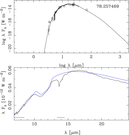
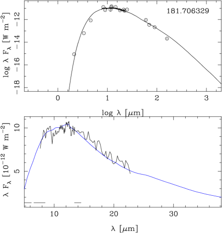
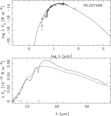
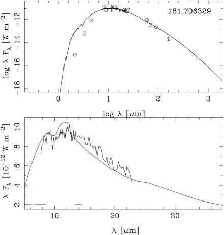
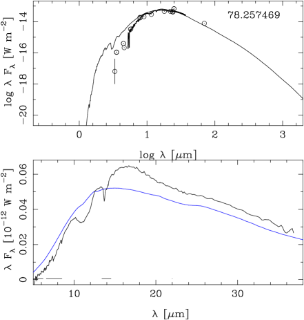
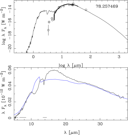
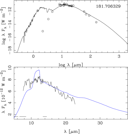
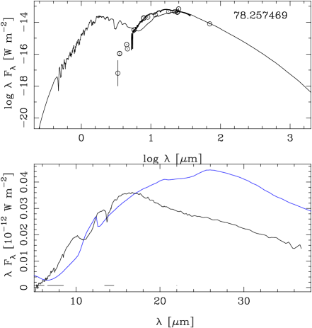
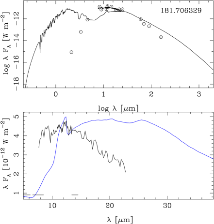
Figure 6: Predicted SEDs and MIR spectra as a function time for two stars (left-hand and right-hand panels) when the MLR stops abruptly and the CSE expands at 10 km s^-1. From top to bottom the SED at $t$=0, and after 30, 50, 200, and 500 years.

6.7 MIR spectra of mass-losing carbon stars as a tracer of interstellar extinction

As part of the fitting of the SEDs and MIR spectra, the observed photometry and spectra were corrected for IS extinction, including, in the MIR regime, the local ISM model of Chiar & Tielens (2006), using a ratio of $A_{\rm V}/A_{\rm K}=0.118$ to scale it to the adopted reddening law of Cardelli et al. (1989) with the improvements by O’Donnell (1994) from the UV to the NIR in MoD (Groenewegen, 2012). In this model, the extinction is smallest near 7.5 $\mu$m ($A_{\rm 7.5\leavevmode\nobreak\ \mu m}/A_{\rm K}=0.38$) and has a peak at the silicate feature ($A_{\rm 9.8\leavevmode\nobreak\ \mu m}/A_{\rm K}\approx 1.0$). In other words, for $A_{\rm V}\approx 8.5$ the extinction becomes $A_{\rm 9.8\leavevmode\nobreak\ \mu m}\approx 1.0$, which should be noticeable in an MIR spectrum.

Figure 7 shows this very clearly where the SEDs and MIR spectra are shown for three stars with estimated $A_{\rm V}$s (see Appendix C on how $A_{\rm V}$ was determined) of 2.4, 4.3, and 5.7 mag, respectively, and with no correction. Not only is the IS 9.8 $\mu$m feature very evident, but the MIR spectrum is better fit over the entire wavelength range. The difference in the SEDs in the upper panels appears quite small in the optical, and this is due to the fact that luminosity and optical depth were refitted in the models with no IS extinction.

The principle of using MIR spectra to trace (MIR) interstellar extinction works for every type of star of course but the highly mass-losing C-stars have an advantage as they are bright in the MIR and have no strong intrinsic features near 10 $\mu$m. The same three stars without mass loss would be 4.0-4.6 mag fainter in the $N$-band. The same would be the case when using normal (O-rich) red giants, while when using MIR brighter mass-losing O-rich stars one would have to distinguish between the circumstellar and IS silicate features which would be extremely challenging.

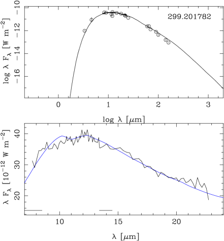
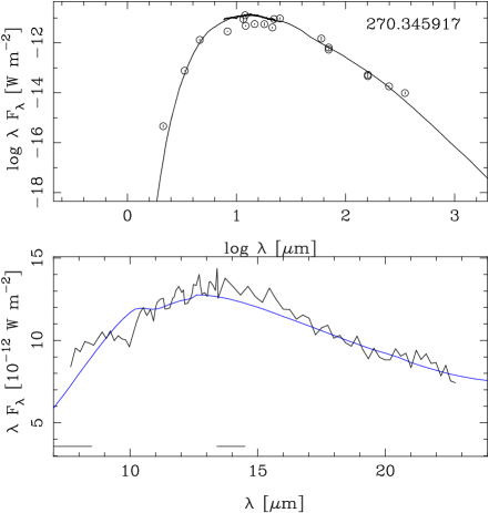
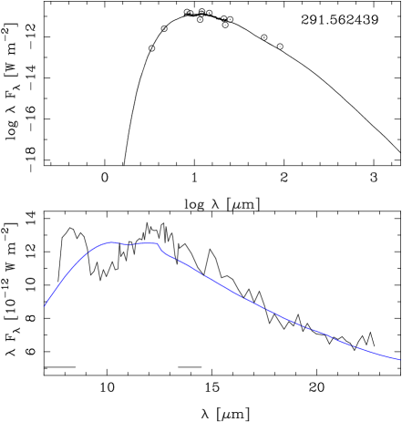
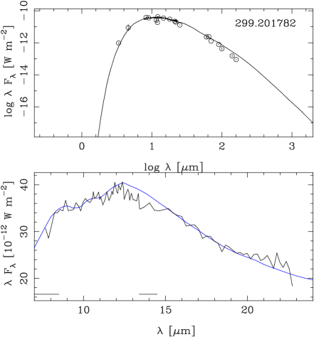
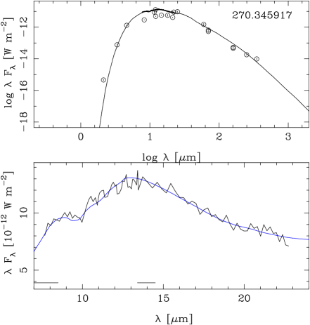
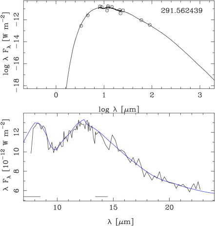
Figure 7: Effect of 9.8 $\mu$m silicate IS extinction feature. The top panels show the fits to the SEDs and MIR spectra without IS extinction correction ($A_{\rm V}$ = 0), while the bottom panels show the fits for three stars with, from left to right, $A_{\rm V}$ = 2.4, 4.3, and 5.7 mag, respectively. The luminosity and optical depth were refitted in the case of $A_{\rm V}$ = 0 and that is the reason that the difference in the SEDs appears small.

7 Final remarks

The period analysis of the WISE/NEOWISE time series data of 1775 objects colour selected to include known C-rich objects with flat MIR continua or SiC in absorption and known Galactic O-rich AGB stars with pulsation periods over 1000 days, supplemented with 217 AGB stars in the MCs previously studied in the $K$-band, is presented. In addition, periods from the literature and in many cases a reanalysis of time series data from other surveys is presented. The SEDs and MIR spectra were modelled with a dust RT programme for a subset of 316 stars as well. The results are presented in the seven subsections of Sect. 6. This includes the detection of new C-rich EROs and new LPVs, of which 145 have periods $>$1000 days.

The nature of the C-rich EROs remains uncertain. Most of the objects in the MCs follow a $PL$ relation and this relation was used to estimate the distance to the Galactic EROs with a period. However, a significant fraction of galactic sources show variability not consistent with an AGB nature (implausibly long periods or no variability). A P-AGB nature for some EROs is difficult to exclude, but given the lifetimes, one would expect a larger number of SEDs with double-peaked SEDs. A possibility is that the shape of some of the SEDs is linked to an aspherical CSE, which is possibly linked to binarity. High spatial resolution line and continuum observations in the MIR or (sub-)mm would be helpful to better characterise the CSE of some of these objects.

In general, distance determinations to these red sources are crucial as well as is investigating and understanding their nature, in particular for the ERO sources. The $PL$ relation is the only available method at the moment, but this has clear limitations. The targets studied here are ideal candidates for an IR astrometric mission (Hobbs et al., 2021). Of the 150 (candidate) EROs in our Galaxy about 85% have $K<$20 mag. Going to even slightly redder wavelengths would be even more advantageous as all Galactic ERO candidates have $L<$14.3 for example.

Appendix A Basic data and results from the period analysis

Tables LABEL:WISEREALSam, LABEL:WISEREALPer, LABEL:noWISESambutREAL, LABEL:noWISEPerbutREAL, LABEL:WISESamnotREAL, LABEL:WISEPernotREAL contain the basic data and the results of the period analysis.

1]

Table 3: Sample of bona fide stellar sources with a period analysis based on WISE data, general information (first entries).

Ra	Dec	Identifiers	Dist	ObjType	2M	GLP	Aka	MSX	MGL	HGL	$V_{\rm b}$	$V_{\rm r}$	LRS	Spec. Type	Comment
(deg)	(deg)		(″)		(″)	(″)	(″)	(″)	(″)	(″)	(km s-1)	(km s-1)
19.463942	67.231448	IRAS01144+6658 RAFGL190	0.22	C			1.1	1.7			nd	nd	U
124.826307	-21.737399	IRAS08171-2134 RAFGL5250	0.30	C	0.3		0.1				-	-	U
237.773837	-56.890007	IRAS15471-5644	0.20	Can.C	0.2		1.2	0.9			nd	nd	U
287.486914	9.447611	IRAS19075+0921 RAFGL2333	0.03	C	0.0		1.2	0.8		1.6	-	-	U
323.345002	56.743063	IRAS21318+5631 RAFGL5625S	0.51	C			1.1	0.5			nd	nd	U	C
349.802533	17.192628	IRAS23166+1655 RAFGL3068	0.33	C	0.3		0.7				-	-		C
89.161446	-67.892776	IRAS05568-6753	0.23	C			1.9	3.4			-	-
82.407959	-72.831322	ERO0529379 IRAS05305-7251	0.17	C			0.7	1.4			-	-			q(6)
87.608788	-69.934212	ERO0550261 IRAS05509-6956	0.16	C			0.8	0.7			-	-			q(6)
79.701599	-69.559563	ERO0518484 IRAS05191-6936	0.30	C			1.5	3.1			-	-
87.249886	-70.556229	IRAS05495-7034	0.77	AGB			0.6				-	-
75.631233	-68.093285	ERO0502315 SSTISAGE1CJ050231.47-680535.9	0.04	AGB			1.1	3.3			-	-
76.023376	-68.394501	ERO0504056 IRAS05042-6827	0.16	C			1.1				-	-
81.419411	-70.140877	ERO0525406 IRAS05260-7010	0.15	C			0.4	2.3			-	-
78.257469	-69.564110	IRAS05133-6937	0.28	C			0.8				-	-
79.548790	-70.507469	ERO0518117 IRAS05187-7033	0.12	C			0.7				-	-
82.684006	-71.716766	IRAS05315-7145	0.32	AGB			0.6				-	-			q(6)
281.468597	-1.778703	IRAS18432-0149 OH30.7+0.4	1.31	OH/IR			1.3	0.8		1.3	49.5	84.1	A
282.174774	-2.841357	IRAS18460-0254 OH30.1-0.7 RAFGL5535	0.06	OH/IR			1.0	1.0		1.2	78.5	118.9
282.859344	-1.064581	IRAS18488-0107 OH32.0-0.5	0.36	OH/IR			0.6	0.8		0.7	55.2	95.8	A
283.092775	-0.236713	IRAS18498-0017 OH32.8-0.3 RAFGL5540	0.37	OH/IR	0.4		0.8	1.0		1.5	45.6	76.0	H
287.284637	8.276116	GPSR042.309-0.133	0.78	Radio			1.7	1.2		0.3	42.3	75.3
23.463343	62.448162	IRAS01304+6211 OH127.8-0.0 RAFGL230	0.19	OH/IR	0.2		0.2	0.2			-65.2	-43.0	A
53.377491	60.335957	IRAS03293+6010 OH141.7+3.5 RAFGL5097	0.61	Mira	0.1		0.8				-69.1	-44.9	A
79.197746	45.567860	IRAS05131+4530 RAFGL712	0.22	OH/IR	0.2						nd	nd	F
111.101738	-20.198791	IRAS07222-2005	0.45	Star	0.4		0.6	1.5			76.9	93.2	E	M9:
266.099701	-31.927624	IRAS17411-3154 RAFGL5379	4.13	OH/IR				0.7		0.6	-39.2	-2.7
280.309784	-6.250149	IRAS18385-0617 OH26.2-0.6	0.22	OH/IR	0.2		2.0	1.3		0.9	49.8	93.0
277.128905	-9.970644	IRAS18257-1000 OH21.5+0.5	0.00	OH/IR			1.1	0.7		1.8	97.6	134.0
51.285198	65.535362	IRAS03206+6521 OH138.0+7.2 RAFGL5093	0.35	OH/IR	0.4		0.6				-46.4	-27.6	A
0.441592	62.748863	IRAS23592+6228	2.27	Star	0.1		0.9	1.4			-	-	F
3.853554	54.906147	IRAS00127+5437	0.21	Star	0.1		0.2				-	-	E
4.963700	65.991821	IRAS00170+6542	0.20	Can.PAGB	0.1		1.2	1.5			-65.0	-37.6	E

Table 3: continued.

2]

Table 4: Sample of bona fide stellar sources with a period analysis based on WISE data, period information (first entries).

Ra	Dec	Periods literature	P refit	$P1$	$\sigma_{\rm P1}$	$P2$	$\sigma_{\rm P2}$	Amp1	$\sigma_{\rm A1}$	$W1$	$\sigma_{\rm W1}$	$\chi_{\rm r,W1}^{2}$	Amp2	$\sigma_{\rm A2}$	$W2$	$\sigma_{\rm W2}$	$\chi_{\rm r,W2}^{2}$	Com	Class
(deg)	(deg)	(d)	(d)	(d)	(d)	(d)	(d)	(mag)	(mag)	(mag)	(mag)		(mag)	(mag)	(mag)	(mag)
19.463942	67.231448	1060 (24)		1053	4.1	1042	4.2	1.85	0.13	8.874	0.019	139.9	1.52	0.05	4.767	0.026	2.2		ERO LPV
124.826307	-21.737399			944	7.4	937	5.8	1.52	0.09	7.251	0.059	50.0	1.39	0.08	3.811	0.047	2.1		ERO LPV
237.773837	-56.890007	no (8) 453 (3)	925 $\pm$ 3 (43)	942	7.6	974	11.4	1.43	0.09	7.321	0.057	42.6	1.49	0.15	3.718	0.061	4.2		ERO LPV
287.486914	9.447611			1068	8.9	1075	9.7	1.19	0.06	6.144	0.078	9.7	1.55	0.12	2.496	0.062	1.9		ERO LPV
323.345002	56.743063			924	4.3	962	9.6	1.14	0.04	7.390	0.022	40.1	1.51	0.14	3.700	0.066	7.0		ERO LPV
349.802533	17.192628	696. (28) 520? (26) 700. (22)		747	4.6	705	674.4	0.89	0.04	5.283	0.032	1.7	0.63	2.01	1.813	2.042	6.0		ERO LPV
89.161446	-67.892776	1197 $\pm$ 32 (1) 1209 (2)		1223	1.2	1217	1.3	1.24	0.04	11.978	0.003	37.3	1.02	0.05	8.971	0.002	80.4		ERO LPV
82.407959	-72.831322	680 (2)		679	1.0	677	1.1	0.62	0.01	14.119	0.008	7.9	0.61	0.02	10.709	0.006	38.6		ERO LPV
87.608788	-69.934212	1052 (2)		1104	4.1	1113	2.6	0.65	0.01	15.485	0.012	2.8	0.72	0.03	11.466	0.005	35.4		ERO LPV
79.701599	-69.559563	no (2)						0.00	0.00	15.307	0.070	0.3	0.00	0.00	12.700	0.015	10.2		ERO
87.249886	-70.556229	no (2)		4453	1288	3429	98.6	0.06	0.05	15.502	0.011	2.1	0.12	0.01	13.502	0.007	1.6		ERO
75.631233	-68.093285	no (2)		1739	111.8	1890	20.7	0.76	0.26	15.662	0.125	19.8	0.31	0.02	13.074	0.007	4.4		ERO LPV
76.023376	-68.394501	no (2)						0.00	0.00	16.213	0.140	0.2	0.00	0.00	13.194	0.007	4.5		ERO
81.419411	-70.140877	no (2)						0.00	0.00	15.703	0.351	4.4	0.00	0.00	13.313	0.016	5.2		ERO
78.257469	-69.564110	no (2)				9094	3214	0.00	0.00	15.547	0.087	0.1	0.28	0.15	13.871	0.046	1.2		ERO
79.548790	-70.507469	no (2)		8188	2519	4666	81.4	0.63	0.34	14.815	0.285	2.5	0.48	0.01	11.941	0.004	4.2		ERO LPV
82.684006	-71.716766	no (2)		969	16.4	944	13.8	0.05	0.02	13.812	0.004	2.8	0.04	0.00	11.957	0.003	2.4		ERO
281.468597	-1.778703	1140 $\pm$ 30 (31)		1176	43.1	1125	17.4	1.05	0.10	5.754	0.184	31.7	1.35	0.10	2.518	0.106	0.5		LPV
282.174774	-2.841357	2013 $\pm$ 243 (32) 1730 $\pm$ 200 (31) 2173 (30)		1952	45.9	1524	16.8	0.67	0.06	7.430	0.031	8.0	0.88	0.08	2.966	0.053	1.3		LPV
282.859344	-1.064581	1417 $\pm$ 108 (32) 1519 (30) no (4)		1632	14.0	1605	21.6	0.89	0.07	7.506	0.060	9.0	1.34	0.12	3.400	0.068	2.5		LPV
283.092775	-0.236713	1539 $\pm$ 31 (32) 1750 $\pm$ 130 (31) 1691 (30) no (4)		1436	32.6	1666	25.8	0.67	0.07	7.296	0.048	10.5	1.32	0.13	2.694	0.087	2.8		LPV
287.284637	8.276116			2475	69.6	1976	51.4	0.68	0.09	7.659	0.056	73.0	0.88	0.15	4.566	0.100	5.0		LPV
23.463343	62.448162	759 (12) 1540 $\pm$ 16 (21) 1638 $\pm$ 57 (32) 1592 (30)						0.00	0.00	3.864	0.024	2.1	0.00	0.00	1.445	0.054	0.5
53.377491	60.335957	1800 $\pm$ 400 (25) 2210 (30)		1445	45.2	1833	293.3	0.62	0.09	4.502	0.097	2.4	0.33	0.29	2.418	0.152	5.7		LPV
79.197746	45.567860	1100 $\pm$ 100 (25) 1051 (30)		1182	16.0	1133	35.3	1.05	0.09	4.439	0.057	2.0	0.72	0.16	2.404	0.099	3.6		LPV
111.101738	-20.198791	5746/1411 (6) 1200 $\pm$ 200 (25) 7 (4)		1447	24.3	1488	21.0	0.62	0.10	4.016	0.104	0.8	1.09	0.11	2.999	0.082	3.8		LPV
266.099701	-31.927624	1440: (25) 1440 (33) 1 (3)	1766 $\pm$ 47 (43)	2054	58.6			0.72	0.11	4.086	0.134	0.8	0.00	0.00	0.708	0.106	0.0	1	PER
280.309784	-6.250149	1172 $\pm$ 94 (32) 1330 $\pm$ 50 (31)		1372	22.3	1206	66.3	0.62	0.09	4.485	0.120	0.4	0.48	0.16	2.468	0.132	2.4		LPV
277.128905	-9.970644	1785 $\pm$ 114 (32)		1548	96.5	1702	67.1	1.59	0.19	8.564	0.142	99.5	1.64	0.15	3.848	0.075	3.4		LPV
51.285198	65.535362	1276 $\pm$ 150 (32) 1410 (30)		1431	26.2	1300	77.7	0.53	0.05	4.075	0.059	0.8	0.30	0.12	2.009	0.103	1.5		LPV
0.441592	62.748863			731	1.5	720	3.8	1.02	0.03	5.201	0.015	0.9	1.06	0.07	3.209	0.036	2.5		LPV
3.853554	54.906147			613	6.4	627	6.4	0.46	0.04	3.738	0.033	0.6	0.59	0.12	2.268	0.079	2.9		LPV
4.963700	65.991821							0.00	0.00	3.746	0.037	2.8	0.00	0.00	2.475	0.047	3.1		nvoh

Table 4: continued.

3]

Table 5: Sample of bona fide stellar sources with a period analysis based on literature data, general information.

Ra	Dec	Identifiers	Dist	ObjType	2M	GLP	Aka	MSX	MGL	HGL	$V_{\rm b}$	$V_{\rm r}$	LRS	Spec. Type	Comment
(deg)	(deg)		(″)		(″)	(″)	(″)	(″)	(″)	(″)	(km s-1)	(km s-1)
353.614540	43.550311	IRAS23320+4316 IRC+40540 RAFGL3116	0.39	C	0.4		0.8				-	-	C	C C8,3.5e J M8+
284.625305	6.715967	IRAS18560+0638 RAFGL2290	0.39	OH/IR	0.4		0.5	2.3			2.4	34.8	A
334.864610	59.856052	IRAS22177+5936 NSV25875 RAFGL2885	0.22	OH/IR	0.2		1.0	2.6			-39.8	-10.0	A
279.385437	-5.399753	IRAS18348-0526 OH26.5+0.6 RAFGL2205	0.10	OH/IR	0.1			1.0		0.5	12.8	39.9	A
6.921023	69.647507	IRAS00247+6922 RAFGL67	0.75	C	0.6		0.6				-	-	C	C:
75.878654	-69.966820	IRAS05039-7002	0.48	Star			0.5				-	-
77.845406	-11.848938	IRAS05090-1154 RAFGL702 RXLep	0.66	AGB	0.7		0.2				nd	nd		M6III M7 M7II:
79.323730	53.586071	IRAS05132+5331 RAFGL715 RAur	0.19	S	0.4		1.5				nd	nd	E	M10 M6+e M7.5Se M9e
82.525955	-70.511375						1.5	1.3			-	-			q(6)
85.957069	32.701687	IRAS05405+3240 RAFGL809	0.15	C	0.3		0.7	1.5			nd	nd	C
86.374641	29.118120	IRAS05423+2905	0.24	OH/IR	0.2		0.4	0.5			-	-	E	M10.5 M9
88.954704	20.175150	IRAS05528+2010 RAFGL837 UOri	0.58	Mira	0.5		0.5	2.4			-41.2	-40.7	E	M6e M7e M8+e M9.5
97.072632	-13.053068	HD45677 IRAS06259-1301 RAFGL5195	0.17	Be*	0.2		0.6				nd	nd	E	B0e B2e B2IV/V[e]
97.397789	8.788045	IRAS06268+0849 RAFGL5196 V477Mon	0.58	C	0.5		1.3	1.9			-	-	C	C	q(2)
99.136795	38.445480	IRAS06331+3829 RAFGL966 UUAur	0.13	C	0.2		0.3				-	-	C	C5,3 C6,4 C7,4 N0 N3
99.226021	3.424734	IRAS06342+0328 RAFGL971	0.36	C	0.4		1.5	3.2			-	-	C	C5,9e	q(2)
105.929901	-11.551617	IRAS07013-1128 RAFGL1059 ZCMa	0.48	Ae	0.5		0.4	0.8			-	-	U	Beq Bneq+F F8III/IV[e]
108.111450	8.517594	IRAS07097+0836	0.06	IR			0.2				-	-
111.014603	-12.874392	IRAS07217-1246 RAFGL5230	0.50	C	0.5		1.0	0.4			-	-	C	C
112.697861	-9.776847	IRAS07284-0940 RAFGL1135 UMon	0.24	RVTau	0.3		0.3	0.9			-	-	E	F8Ibe G0I G2Ie G5 G8 K2
118.454765	-53.920090										-	-
139.178528	-47.939484	[LLN92]IRS49-1	1.60	IR				3.1			-	-	H
148.891602	-77.287849	HD86774 IRAS09555-7702	0.48	Star	0.3		0.5				-	-		M1III
149.819809	-56.911324						1.0	3.1			-	-
159.787247	-77.956032	EZCha IRAS10383-7741	0.35	LPV	0.4		1.0				-	-	E	M5/7
161.142731	-60.092995						1.6	2.6			-	-
182.255554	-63.264767						2.6	4.8		3.4	nd	nd	H
184.390961	-67.960808	epsMus IRAS12148-6741 RAFGL4149	2.53	LPV			1.1				-	-	S	M3 M3/5III M4III M5III
205.221130	-61.762733	IRAS13374-6130	1.50	HII			1.5				-	-
205.756912	-62.147499	IRAS13395-6153 RAFGL4176	0.39	IR	0.4			0.4		0.0	-	-
207.907654	-61.652130	IRAS13481-6124	0.20	YSO	0.2		0.6	0.6		3.1	-	-	A
211.898087	-61.455872	[HJF2013]G311.899+00.083	1.02	denseCore	0.6	0.4					-	-	H
216.240234	-60.378918	PMNJ1424-6022	2.17	HII		3.0	1.7	1.9			-	-	H
220.506821	-60.506161	[MHL2007]G316.1386-00.50091	2.06	Can.YSO		2.6		2.1			-	-	H
227.501114	-58.294167						0.9	4.6			-	-	H
237.410202	-54.639774	IRAS15457-5429	2.82	HII				2.4		4.3	-	-	H
237.682434	-53.345341	IRAS15469-5311	0.18	PAGB	0.3		0.4	0.3		1.6	-45.8	-36.3	F
240.578812	-52.924671	IRAS15584-5247	2.32	HII		1.4	2.8	2.7			-	-	P
242.593582	-52.100525	MSX5CG330.8849-00.3703	2.39	IR			2.0				-	-	H
242.660965	-49.097557	SFO76	0.85	Cloud				1.3			-	-	P
242.891373	-48.330719	IRAS16079-4812	0.35	C	0.3		0.6	0.4			-	-	C	C
244.379456	-50.541546	IRAS16137-5025	2.20	HII				3.0		3.6	-	-	P

Table 5: continued.

4]

Table 6: Sample of bona fide stellar sources with a period analysis based on literature data, period information (first entries).

Ra	Dec	Periods literature	P refit	$P1$	$\sigma_{\rm P1}$	$P2$	$\sigma_{\rm P2}$	Amp1	$\sigma_{\rm A1}$	$W1$	$\sigma_{\rm W1}$	$\chi_{\rm r,W1}^{2}$	Amp2	$\sigma_{\rm A2}$	$W2$	$\sigma_{\rm W2}$	$\chi_{\rm r,W2}^{2}$	Com	Class
(deg)	(deg)	(d)	(d)	(d)	(d)	(d)	(d)	(mag)	(mag)	(mag)	(mag)		(mag)	(mag)	(mag)	(mag)
353.614540	43.550311	620. (26) 59 (4)	686 $\pm$ 21 (71)
284.625305	6.715967	1430 $\pm$ 27 (32) 1260 (30)
334.864610	59.856052	1460 $\pm$ 24 (32) 1749 (30)
279.385437	-5.399753	1556 (27) 1589 $\pm$ 42 (32) 1559 $\pm$ 7 (21) (1500) (33) 1592 (30)
6.921023	69.647507	650. (26)	637 $\pm$ 55 (71)
75.878654	-69.966820																		ero
77.845406	-11.848938	/827 (7)
79.323730	53.586071	514/819 (7) 461 (4) 456 $\pm$ 36 (5)
82.525955	-70.511375	808 $\pm$ 4 (1) 806 (2)																	ero
85.957069	32.701687	683: $\pm$ 160 (29) 780. (26)	606 $\pm$ 85 (71)
86.374641	29.118120	508/508 (7) 708/498 (6) 449 $\pm$ 69 (29) 455 $\pm$ 50 (5)
88.954704	20.175150	370/122 (7) 376 (11) 378 (9) 369 (4)
97.072632	-13.053068
97.397789	8.788045	422: (23) no (4)	769 $\pm$ 75 (71)
99.136795	38.445480	429/426 (7)
99.226021	3.424734	653. (28)
105.929901	-11.551617	no (11) 785 (9) no (4)
108.111450	8.517594
111.014603	-12.874392	10 (4)	- (44)
112.697861	-9.776847
118.454765	-53.920090		451 $\pm$ 1 (54)
139.178528	-47.939484
148.891602	-77.287849
149.819809	-56.911324
159.787247	-77.956032	no (7) 62 (9)
161.142731	-60.092995
182.255554	-63.264767
184.390961	-67.960808	no (7)
205.221130	-61.762733
205.756912	-62.147499
207.907654	-61.652130
211.898087	-61.455872
216.240234	-60.378918
220.506821	-60.506161
227.501114	-58.294167
237.410202	-54.639774
237.682434	-53.345341
240.578812	-52.924671	1 (3)
242.593582	-52.100525	no (7)
242.660965	-49.097557
242.891373	-48.330719	710 (8) no (4)
244.379456	-50.541546

Table 6: continued.

5]

Table 7: Sample of likely non bona fide sources, general information (first entries).

Ra	Dec	Identifiers	Dist	ObjType	2M	GLP	Aka	MSX	MGL	HGL	$V_{\rm b}$	$V_{\rm r}$	LRS	Spec. Type	Comment
(deg)	(deg)		(″)		(″)	(″)	(″)	(″)	(″)	(″)	(km s-1)	(km s-1)
1.697865	43.074245										-	-
2.079027	-0.576736										-	-
2.224788	-0.267857										-	-
2.242542	-0.750332										-	-
2.248379	-0.725155										-	-
2.259252	-0.380092										-	-
2.262807	-0.495763										-	-
2.266214	-0.497638										-	-
2.293089	-0.716659										-	-
2.800782	60.514320										-	-	E
6.898109	69.647568										-	-
6.945048	69.648048										-	-
16.626133	12.590879										-	-
19.419439	67.217979										-	-
19.440771	67.231651										-	-
19.454063	67.239548										-	-			q(6)
19.457726	67.212669										-	-
19.466803	67.238457										-	-
19.478022	67.238297										-	-
34.503338	28.621672										-	-
34.506149	28.606207										-	-
34.545307	28.618717										-	-
36.434948	62.061813										-	-
36.437519	62.056862										-	-
36.439510	62.058491										-	-
36.440208	62.060390										-	-
36.685730	62.272881										-	-
36.703152	62.258183										-	-
36.706955	62.260796										-	-
36.715996	62.270233										-	-
36.720409	62.263744										-	-
36.722710	62.260414										-	-
36.732460	62.265739										-	-
36.739769	62.265717										-	-
38.204800	58.044067										-	-
38.217022	58.041882										-	-
38.236389	58.013664										-	-
38.238350	58.016823										-	-
38.242611	58.022480										-	-
38.263523	58.052654										-	-
38.264610	58.054668										-	-
38.264866	58.018578										-	-
38.268902	58.031715										-	-
38.269836	58.038555										-	-

Table 7: continued.

6]

Table 8: Sample of likely non bona fide sources, period information (first entries).

Ra	Dec	Periods literature	P refit	$P1$	$\sigma_{\rm P1}$	$P2$	$\sigma_{\rm P2}$	Amp1	$\sigma_{\rm A1}$	$W1$	$\sigma_{\rm W1}$	$\chi_{\rm r,W1}^{2}$	Amp2	$\sigma_{\rm A2}$	$W2$	$\sigma_{\rm W2}$	$\chi_{\rm r,W2}^{2}$	Com	Class
(deg)	(deg)	(d)	(d)	(d)	(d)	(d)	(d)	(mag)	(mag)	(mag)	(mag)		(mag)	(mag)	(mag)	(mag)
1.697865	43.074245
2.079027	-0.576736
2.224788	-0.267857
2.242542	-0.750332
2.248379	-0.725155
2.259252	-0.380092
2.262807	-0.495763
2.266214	-0.497638
2.293089	-0.716659
2.800782	60.514320
6.898109	69.647568							0.00	0.00	7.883	0.069	351.9	0.00	0.00	5.455	0.093	24.7
6.945048	69.648048
16.626133	12.590879							0.00	0.00	8.506	0.077	500.3	0.00	0.00	4.976	0.290	123.8
19.419439	67.217979
19.440771	67.231651							0.00	0.00	11.707	0.013	10.6	0.00	0.00	9.898	0.024	38.0
19.454063	67.239548							0.00	0.00	12.996	0.008	3.3	0.00	0.00	10.938	0.088	387.0
19.457726	67.212669
19.466803	67.238457
19.478022	67.238297
34.503338	28.621672
34.506149	28.606207
34.545307	28.618717
36.434948	62.061813
36.437519	62.056862
36.439510	62.058491
36.440208	62.060390
36.685730	62.272881							0.00	0.00	11.126	0.013	27.4	0.00	0.00	10.470	0.018	44.3
36.703152	62.258183
36.706955	62.260796
36.715996	62.270233
36.720409	62.263744
36.722710	62.260414
36.732460	62.265739							0.00	0.00	9.977	0.006	1.3	0.00	0.00	9.114	0.015	7.8
36.739769	62.265717							0.00	0.00	9.833	0.005	1.6	0.00	0.00	9.234	0.007	2.2
38.204800	58.044067
38.217022	58.041882							0.00	0.00	15.121	0.071	6.9	0.00	0.00	10.567	0.047	114.5
38.236389	58.013664							0.00	0.00	14.121	0.024	1.7	0.00	0.00	11.015	0.052	106.1
38.238350	58.016823							0.00	0.00	14.989	0.062	8.1	0.00	0.00	10.483	0.062	226.9
38.242611	58.022480							0.00	0.00	13.310	0.057	50.5	0.00	0.00	9.325	0.061	443.6
38.263523	58.052654
38.264610	58.054668							0.00	0.00	14.313	0.029	6.2	0.00	0.00	10.924	0.051	88.0
38.264866	58.018578
38.268902	58.031715
38.269836	58.038555

Table 8: continued.

Appendix B Figures of LCs

Figures 8–18 contain the observed data and fitted LCs, with one figure per separate dataset. Figure 19 shows the LCs of some interesting sources (see Sect. 6.4).

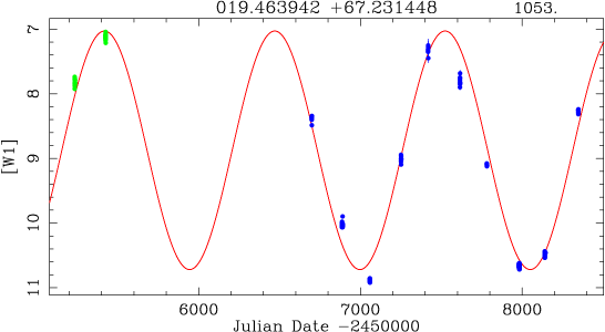
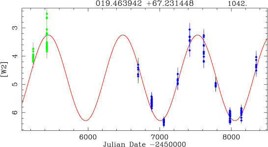
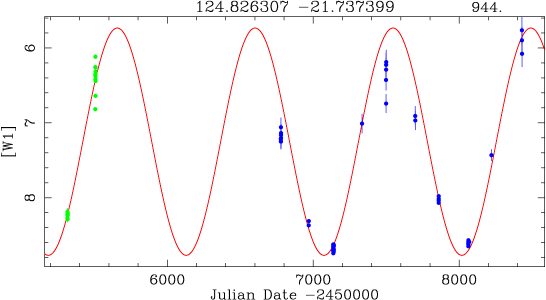
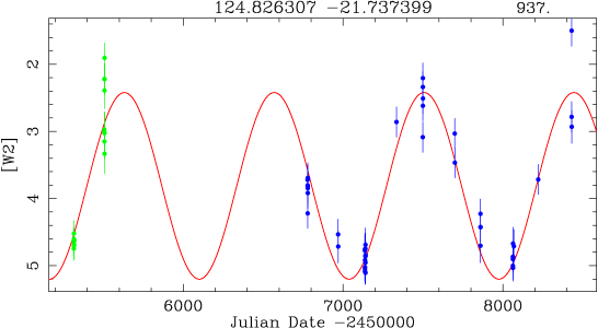
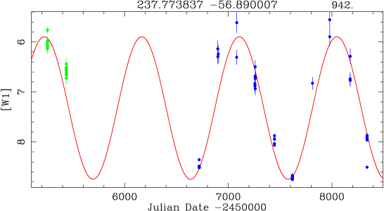
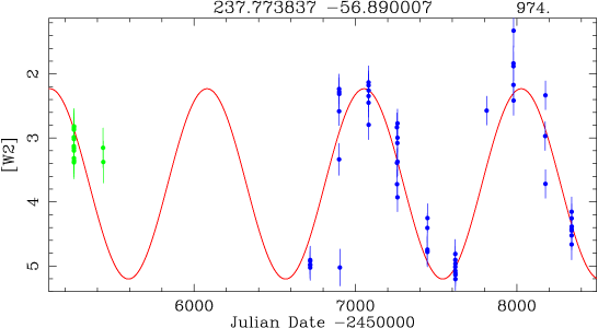
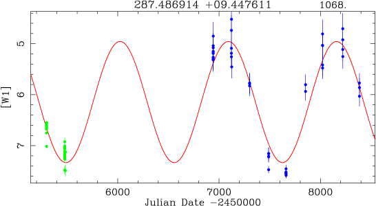
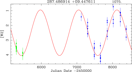
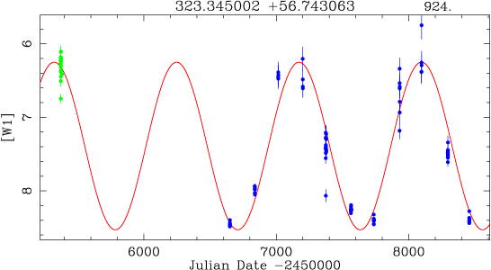
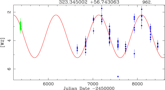
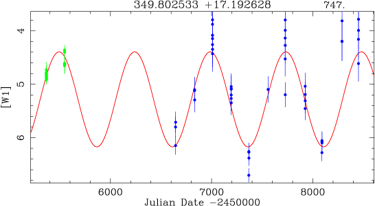
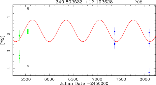
Figure 8: Examples of fits to WISE data (W1 on the left, W2 on the right). The identifier is listed on the top of each panel, with the period to the right. Green points refer to WISE, and blue points to NEOWISE data. Crosses indicate points excluded from the fitting. The complete set of LCs is available at https://doi.org/10.5281/zenodo.5825878.

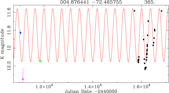
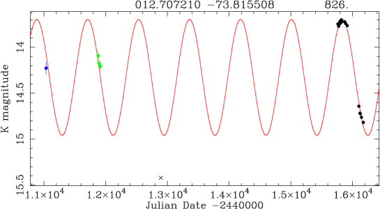
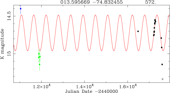
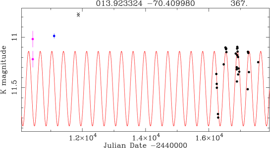
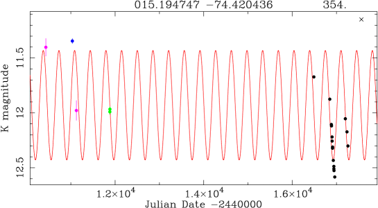
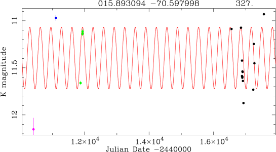
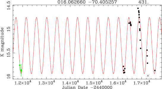
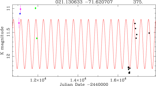
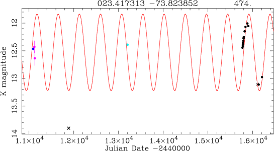
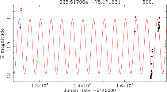
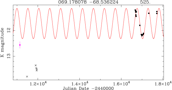
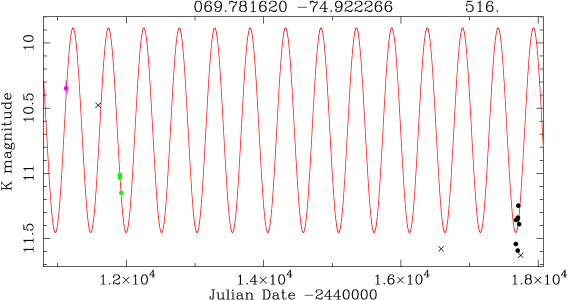
Figure 9: Examples of fits to VMC data $K$-band data. The identifier is listed on the top of each panel, with the period to the right. Data points (with error bars) in black show the VMC, green points represent 2MASS, dark blue points are for 2MASS-6X, light blue points are for the IRSF, and magenta corresponds to DENIS (see Groenewegen et al. 2020).

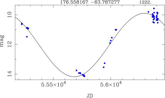
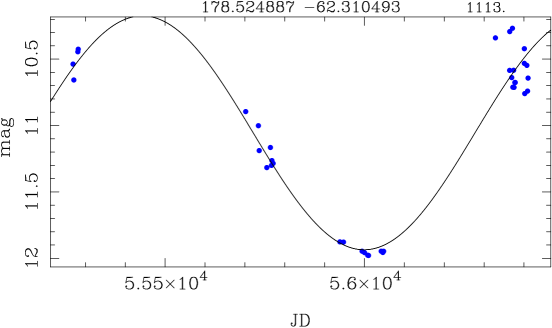
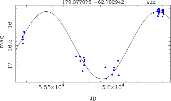
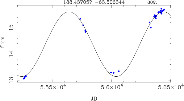
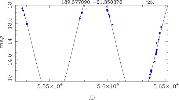
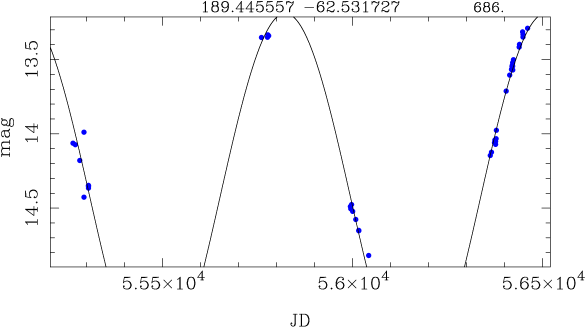
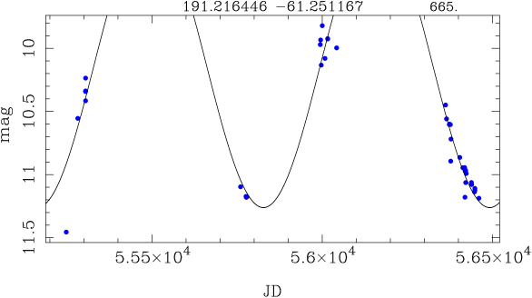
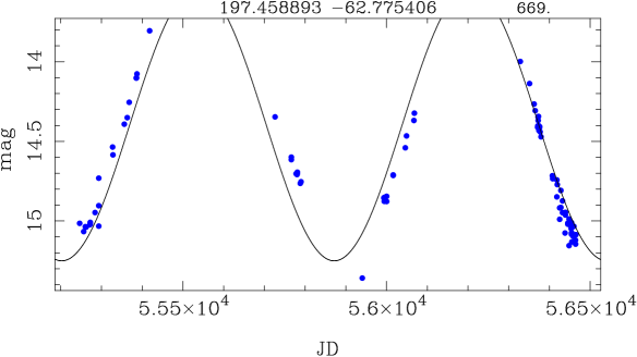
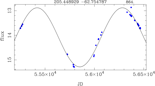
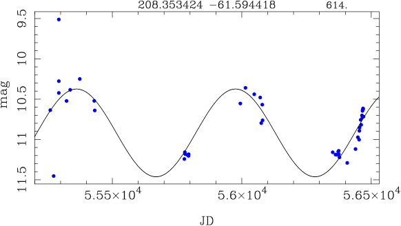
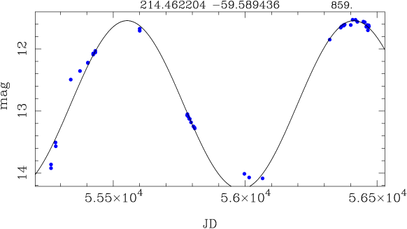
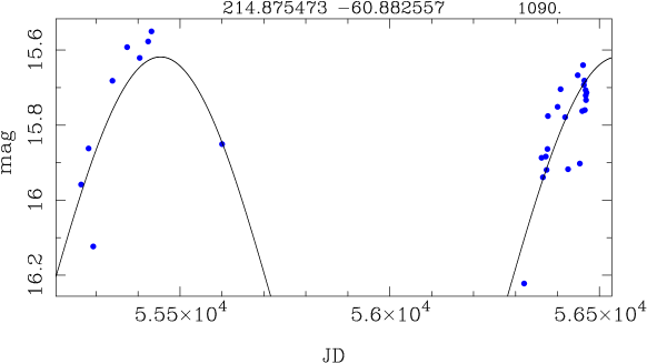
Figure 10: Examples of fits to VVV $K$-band data. The identifier is listed on the top of each panel, with the period to the right.

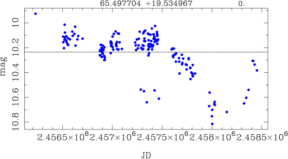
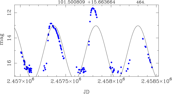
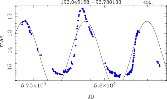
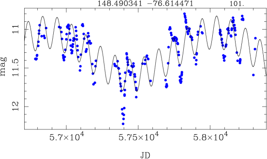
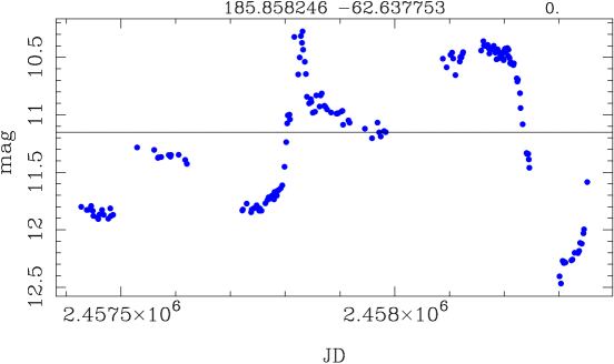
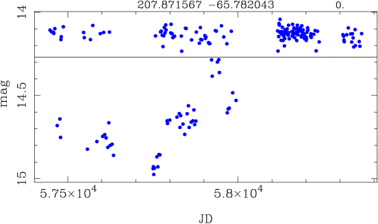
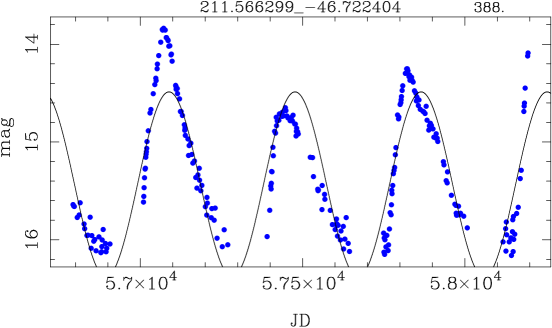
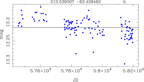
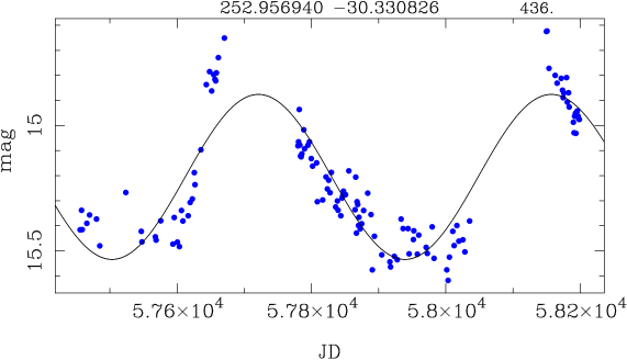
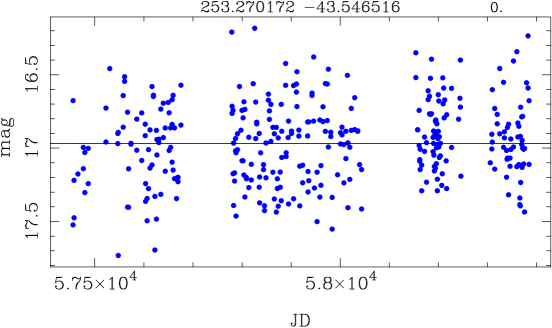
Figure 11: Examples of fits to ASAS-SN $V$-band data. The identifier is listed on the top of each panel, with the period to the right.

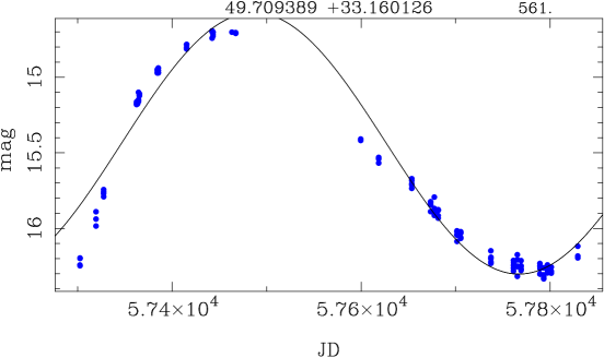
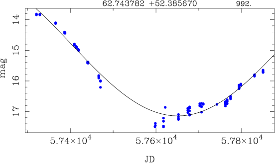
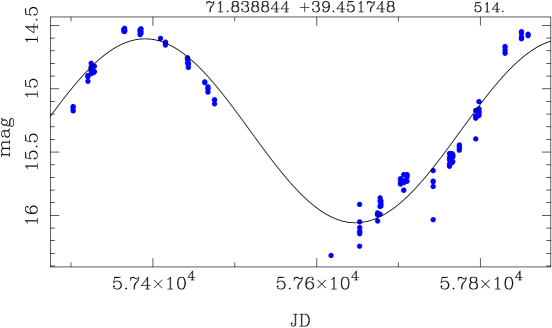
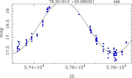
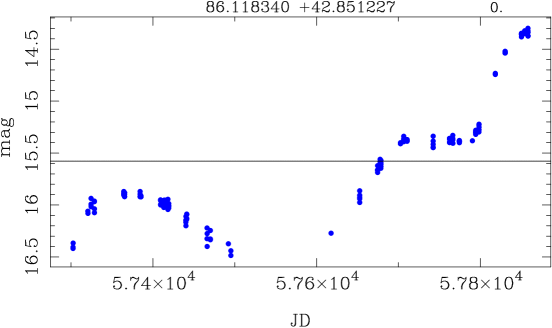
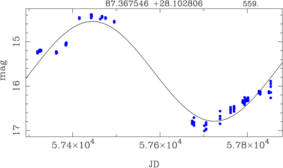
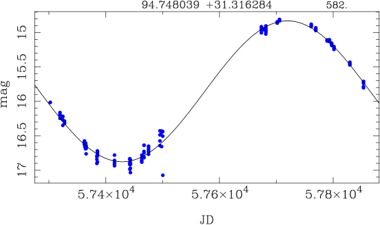
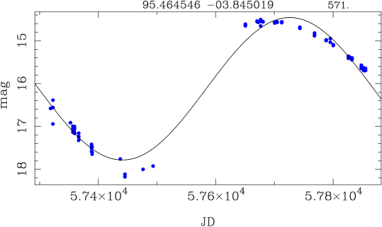
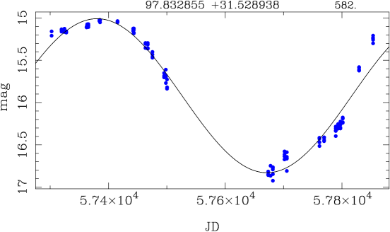
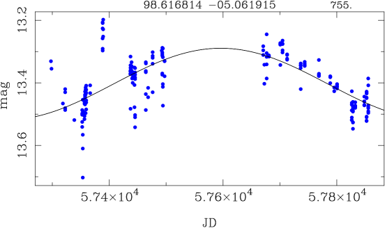
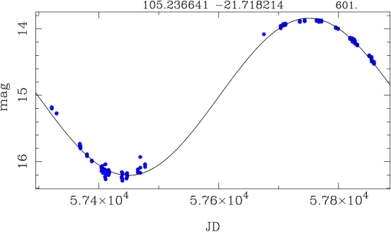
Figure 12: Examples of fits to ATLAS $o$-band data. The identifier is listed on the top of each panel, with the period to the right.

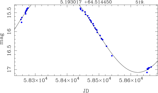
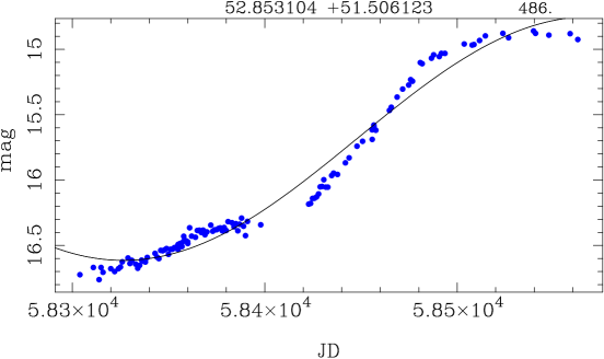
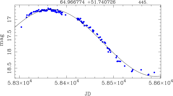
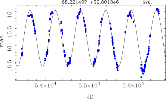
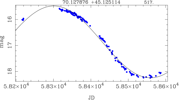
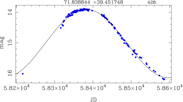
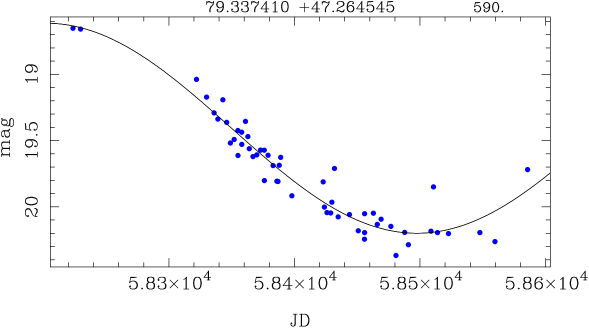
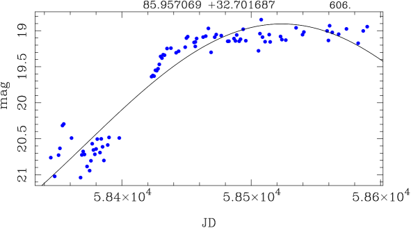
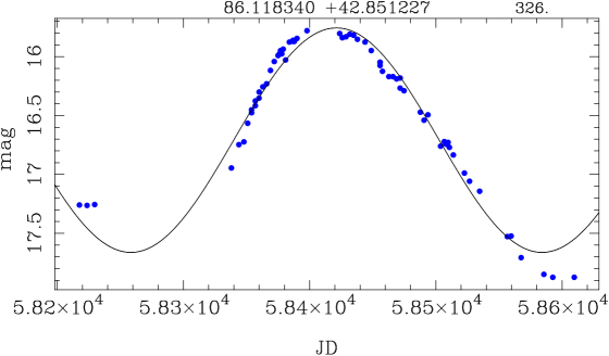
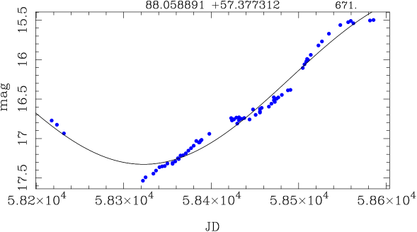
Figure 13: Examples of fits to ZTF $r$-band LCs. The identifier is listed on the top of each panel, with the period to the right.

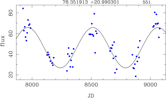
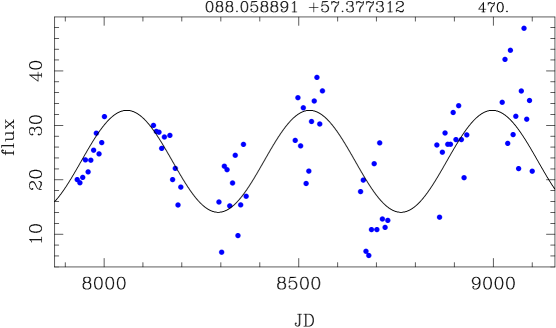
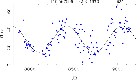
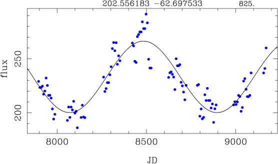
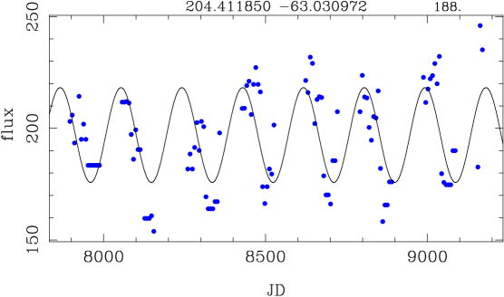
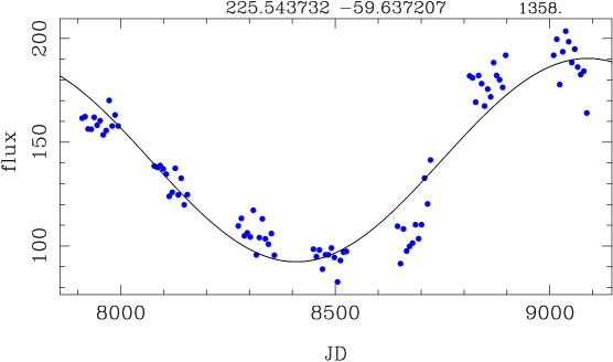
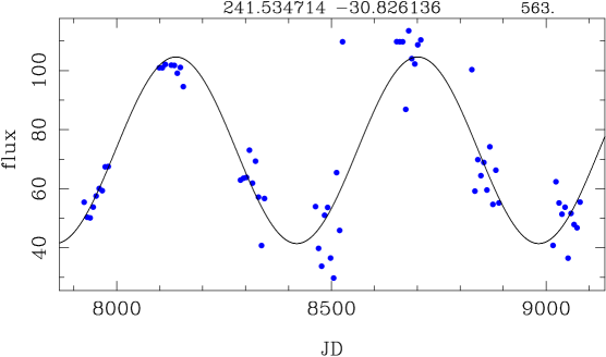
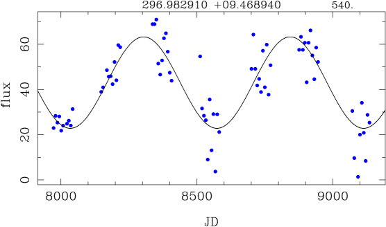
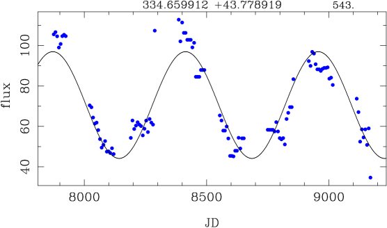
Figure 14: Fits to DIRBE 4.9 $\mu$m flux (in Jy). The identifier is listed on top of each panel, with the period to the right.

Figure 15: Fit to one OMC source in the $V$-band. The identifier is listed on top of each panel, with the period to the right.

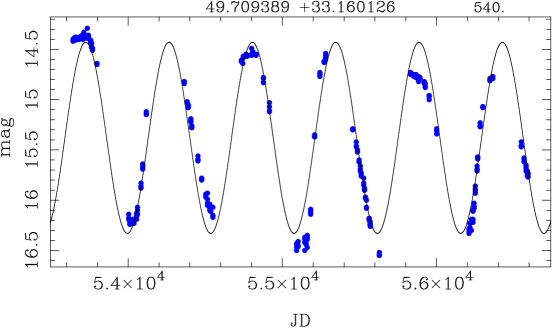
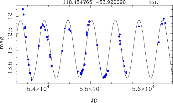
Figure 16: Fits to three CSS sources in the $V$-band. The identifier is listed on top of each panel, with the period to the right.

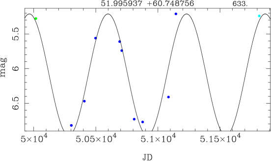
Figure 17: Fits to $K$-band data from Kerschbaum et al. (2006). The identifier is listed on top of each panel, with the period to the right.

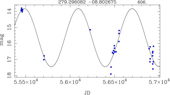
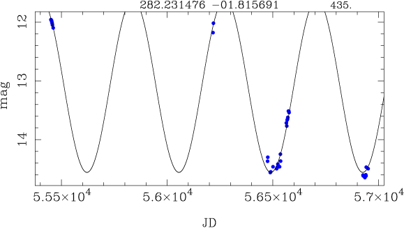
Figure 18: Fits to two GDS sources in the $I$-band. The identifier is listed on top of each panel, with the period to the right.

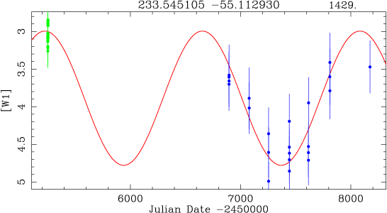
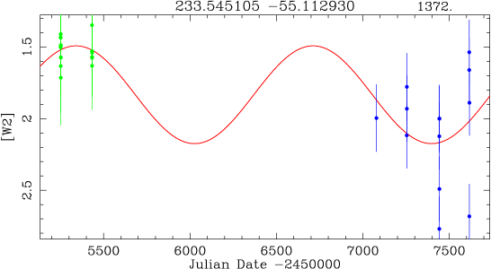
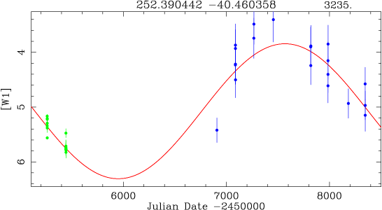
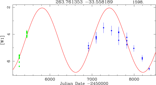
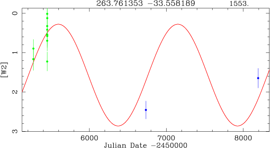
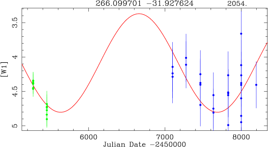
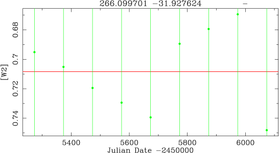
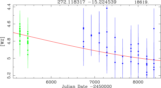
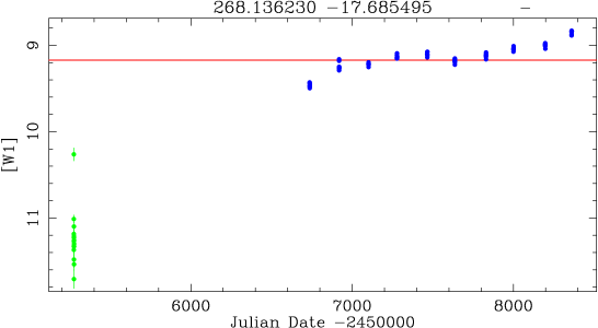
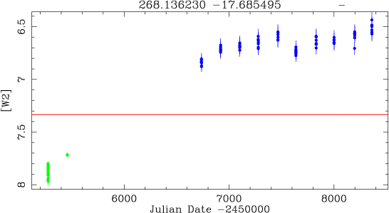
Figure 19: Examples of fits to WISE data of some interesting LCs (see Sect. 6.4. The identifier is listed on the top of each panel, with the period to the right.

Appendix C Constructing and fitting spectral energy distributions

This appendix describes the construction and fitting of the spectral energy distributions (SEDs) of a subset of stars in order to find new C-rich EROs and derive their MLRs. As described in the main text, the intial subsample consisted of stars with W2$-$W3 $>$3.0 based on the colours of the known C-rich EROs in Table 1. Sixty-seven stars with a blue and red detection on the OH maser database of Engels & Bunzel (2015) were removed as these are confirmed O-rich sources.

For the remaining sample of 316 objects, the following databases were queried to collect photometric data: AllWISE (Cutri & et al., 2014), Akari FIS (Yamamura et al., 2010), Akari IRC (Ishihara et al., 2010b), Akari NIR PSC (Kato et al., 2012), IRAC and MIPS observations from the SAGE program (Meixner et al., 2006) and Gruendl & Chu (2009), GLIMPSE (Spitzer Science, 2009), MIPSGAL (Gutermuth & Heyer, 2015b), MSX (Egan et al., 2003b), IRAS Point and Faint Source Catalogue (Joint IRAS Science Working Group, 1986; Moshir & et al., 1990), Herschel PACS (Herschel Point Source Catalogue Working Group et al., 2017), Herschel PACS and SPIRE observations from the Heritage (Seale et al., 2014) and the Hi-GAL programme (Molinari et al., 2016; Elia et al., 2017), VVV (VISTA Variable in the Via Lactea Survey, datarelease 2; Minniti et al. 2017), VMC (VISTA Magellanic Survey, datarelease 4; Cioni et al. 2011), the Large Magellanic Cloud Near-Infrared Synoptic Survey (Macri et al., 2015), the IRSF Magellanic Clouds Point Source Catalogue (Kato et al., 2007), the JCMT Plane Survey (Eden et al., 2017), and ATLASGAL (Csengeri et al., 2014). After inspecting the SEDs and an initial round of model fitting (see below) the literature was searched for additional photometric data for selected sources. Details on the SEDs of individual sources are available upon reasonable request to the author.

In addition, MIR spectra were collected from the IRAS LRS (Volk & Cohen, 1989), the Infrared Space Observatory short-wavelength spectrograph (SWS) from Sloan et al. (2003), and the SST IRS. In the latter case the spectra were retrieved through the CASSIS service (Lebouteiller et al., 2011).

The SEDs and MIR spectra were modelled with MoD (Groenewegen, 2012). The central stars of C-stars are represented by model atmospheres from Aringer et al. (2009), and those for O-stars with MARCS model atmospheres (Gustafsson et al., 2008). For stars hotter than AGB stars PHOENIX model atmospheres (Hauschildt et al., 1999) were used.

For C-stars, the dust composition is a mixture of amorphous carbon (AmC), silicon carbide (SiC), and magnesium sulfide (MgS). For O-stars, the dust composition is a mixture of amorphous silicates and metallic iron. When MIR spectra are available, the distinction between C-rich and O-rich chemistry is in most cases clear and the ratio of SiC/AmC and MgS/AmC is estimated by eye. If no MIR spectra are available, typical ratios (SiC/AMC= 0.05, MgS/AMC= 0.10) are adopted in the fitting. For the O-rich sources, a ratio of metallic iron to amorphous silicates of 0.15 is adopted, which seems to be a reasonable fit in most cases. The actual dust composition may be more complicated, but it is not our aim to study this in detail here. The distinction between C- and O-rich chemistry is then made by fitting the photometry alone, and adopting the best fit.

For a given set of photometry and spectra as input data, MoD determines the best-fitting luminosity (for a given distance), dust optical depth, dust temperature at the inner radius, and slope of the density profile. Any of these parameters can also be fixed.

Canonical distances to the LMC of 50 kpc and 61 kpc to the SMC were adopted, which are well within the error bars of the current best estimates (de Grijs et al., 2014; de Grijs & Bono, 2015). A priori, the distances to the objects in our Galaxy are unknown. However, we make use of the fact that LPVs are expected to follow a $PL$ relation, and that many ERO candidates in the sample are located in the LMC (and a few in the SMC). Figure 20 shows the derived $PL$ relation based on 31 objects and with an rms of 0.31 mag. The functional form is given in the main text, Eq. 2.

Figure 20: Bolometric $PL$ relation for red C-rich objects in the Magellanic Clouds. Stars without a period are plotted as plus signs at $\log P=2.5$. Stars that are excluded from the fit are plotted as open symbols. Circles (two objects) represent stars in the SMC, and the squares are objects in the LMC.

This $PL$ relation was then applied to the ERO candidates in the Galaxy which have a period, to obtain a luminosity, for both C- and O-rich sources. For C-rich ERO candidates in the Galaxy without a period a luminosity of 7100 L_⊙was adopted, which is the median luminosity of C-rich sources in the MCs. O-rich ERO candidates in the Galaxy without a period were placed at an arbitrary distance of 2 kpc. For a few sources with exceptionally long (and or uncertain periods) the $PL$ relation is not applied as it would lead to unrealistically large luminosities incompatible with an AGB status, or, for a few sources at low galactic latitudes, it would lead to large distances with correspondingly large reddenings that are incompatible with the SED. These sources were treated as if no period were available, that is $L=$ 7100 L_⊙ was assumed if it is C-rich, and a distance of 2.0 kpc if it was O-rich. In these cases, the objects may indeed not be LPVs, or the periodicity is not related to pulsation, or the period analysis has led to a spurious result.

Interstellar reddening also needs to be taken into account in the fitting. For the sources in the MCs the recent average values from Skowron et al. (2021) were adopted, that is $A_{\rm V}=0.22$ and $0.10$ mag for LMC and SMC, respectively, adopting $A_{\rm V}=3.1\;E(B-V)$ and $E(B-V)=E(V-I)/1.4$. For the Galactic sources two recent 3D reddening models were used to estimate the reddening in the direction of the stars in the sample. The first is described in Lallement et al. (2018) (hereafter STILISM) and is based on Gaia, 2MASS and APOGEE-DR14 data. For a given galactic longitude, latitude and distance, the tool returns the value of $E(B-V)$ and an error, as well as the distance to which these values refer. If this distance is smaller than the input distance the returned value for the reddening is a lower limit. In these cases, a simple estimate of the reddening at the distance of the source was made. A second reddening value was queried at a distance 0.75 times the maximum distance available in the grid in that direction. Based on this, the first derivative (with an error bar) was determined and the reddening at the distance of the target estimated. Since the total reddening flattens with distance, this estimate is an (severe) overestimate if the distance to the object is (much) larger than the last available grid point in the grid. Therefore, the extrapolated reddening is limited to twice that at the last available grid point (see below).

The second reddening model is that described in Green et al. (2019) and is based on Gaia DR2 data, 2MASS, and Pan-STARRS 1 data. Reddening values are provided out to ‘several’ kpc for stars north of declination $-30\degr$. For 36 sources in overlap and where the distance is available in the STILISM grid, the ratio of the reddening value between STILISM and the Bayestar19 models is 0.94 with quite some spread (a median absolute deviation of 0.18). Given this scatter, no attempt was made to scale the two reddening maps. For over a hundred sources where the reddening is available in the ‘Bayestar19’ map and is extrapolated based on STILISM, it was decided to limit the extrapolated reddening to twice that at the last available grid point. The reddening model of Green et al. (2019) is the preferred one as it extends to larger distances, and it is available for 147 of the Galactic sources. The values from STILISM were adopted for the remaining 120 Galactic sources (with the linear extrapolation of the reddening and the limit to it as just described).

The results of fitting the SEDs and MIR spectra are shown is several Tables and Figures. Figure 21 shows some examples of fits for the C-stars in cases when there is, or not, an MIR spectrum available. The complete set of SED fits for the O- and C-stars is available at https://doi.org/10.5281/zenodo.5825878. Tables 2 and 9 show the result of the fitting. The results for the C-stars are discussed in detail in Section 6.5 in connection with the mass return of C-rich EROs in the solar neighbourhood. For another distance, $L\sim d^{2}$ and $\dot{M}$$\sim d$ to first order (ignoring the dependence of the reddening on distance). A cautionary note is made that the MLRs quoted in the last column assume spherical symmetry. The SEDs of many of the O-rich sources cannot be fitted very well and are incompatible with the spherical model rendering the MLRs estimates highly uncertain.

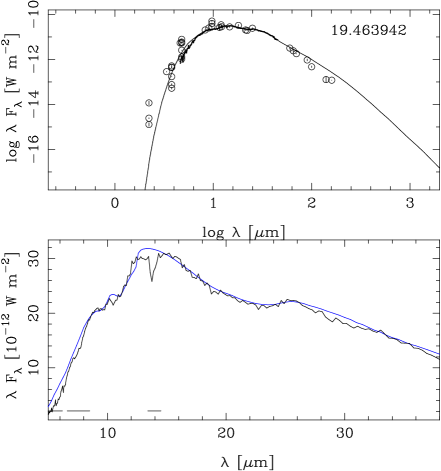
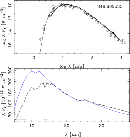
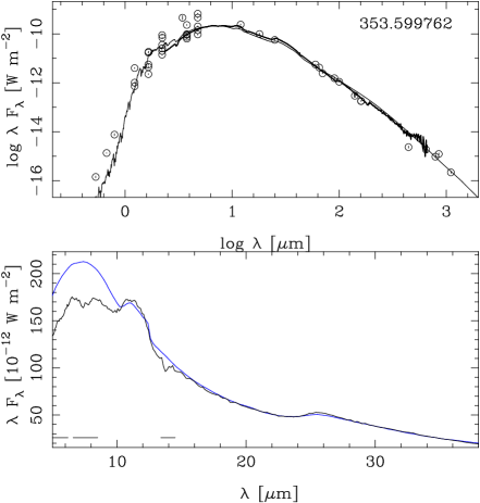
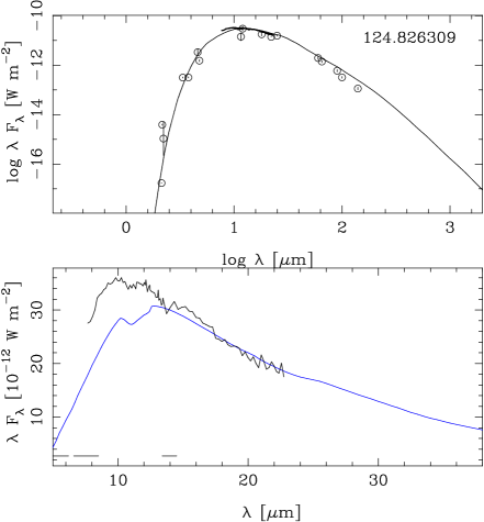
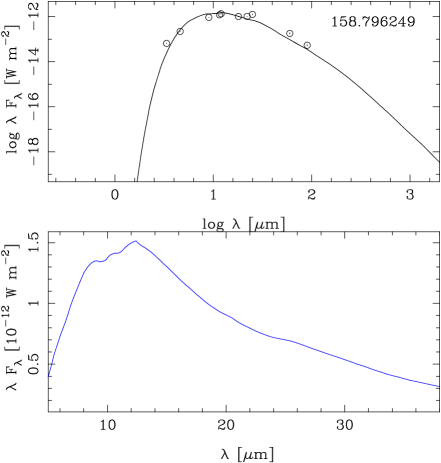
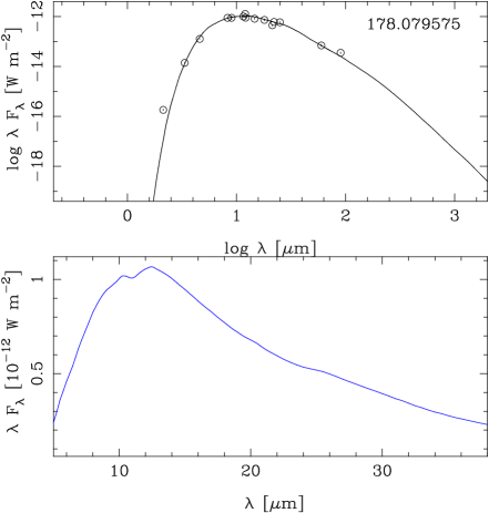
Figure 21: Examples of fits to the SEDs and MIR spectra of some C-stars. The complete set of SED fits for the O- and C-stars is available at https://doi.org/10.5281/zenodo.5825878. To highlight the difference in the dust features, the observations were scaled to the models based on the average flux in the 16-20 $\mu$m region for the C-stars and the 13-15 $\mu$m region for the O-stars in the MIR panels.

Table 9: Fit results of the O-star sample (first entries)

RA	Dec	Period	$d$	$A_{\rm V}$	$T_{\rm eff}$	$L$	$\tau_{0.5}$	$T_{\rm c}$	f	$p$	f	$\dot{M}$
(deg)	(deg)	(days)	(kpc)	(mag)	(K)	(L⊙)		(K)				(M⊙ yr-1)
32.021637	60.767200	-	2.00	2.37	7200	1726 $\pm$ 341	29 $\pm$ 2.1	312 $\pm$ 16	1	1.8 $\pm$ 0.4	1	0.351E-04
83.559708	-69.789062	664	50.00	0.22	30000	253682 $\pm$ 12232	37 $\pm$ 1.6	373 $\pm$ 5	1	1.8 $\pm$ 0.0	0	0.571E-03
84.930687	-69.647270	-	50.00	0.22	10000	1424E3 $\pm$ 132E3	34 $\pm$ 4.0	239 $\pm$ 5	1	2.0 $\pm$ 0.0	0	0.319E-02
85.435890	-2.268356	-	2.00	7.47	12500	1158 $\pm$ 12	23 $\pm$ 0.4	522 $\pm$ 8	1	1.8 $\pm$ 0.0	1	0.105E-04
119.982277	-41.122845	1977	26.94	0.52	5000	48073 $\pm$ 9013	868 $\pm$ 104	1200 $\pm$ 0	0	2.2 $\pm$ 0.0	0	0.740E-03
130.866959	-46.111153	-	2.00	1.22	10000	379 $\pm$ 18	8 $\pm$ 0.2	250 $\pm$ 8	1	1.8 $\pm$ 0.0	0	0.816E-05
137.809174	-45.586235	-	2.00	1.01	7000	1837 $\pm$ 225	34 $\pm$ 0.8	470 $\pm$ 19	1	1.1 $\pm$ 0.1	1	0.392E-05
140.372116	-55.011105	-	2.00	0.94	7600	1604 $\pm$ 130	79 $\pm$ 7.1	552 $\pm$ 36	1	1.4 $\pm$ 0.1	1	0.183E-04
155.062988	-58.053551	936	4.25	0.66	3000	10552 $\pm$ 2697	551 $\pm$ 92.3	1000 $\pm$ 0	0	2.0 $\pm$ 0.0	0	0.182E-03
159.833176	-59.665565	-	2.00	0.87	7600	7549 $\pm$ 2324	91 $\pm$ 8.9	166 $\pm$ 11	1	1.5 $\pm$ 0.0	0	0.626E-03
165.436462	-60.957218	-	2.00	0.90	7600	1902 $\pm$ 326	80 $\pm$ 12.3	270 $\pm$ 18	1	1.5 $\pm$ 0.1	1	0.976E-04
168.056854	-61.279396	-	2.00	0.92	25000	2068 $\pm$ 641	205 $\pm$ 45.8	800 $\pm$ 0	0	1.6 $\pm$ 0.0	0	0.495E-04
169.139252	-61.498360	-	2.00	0.91	3400	2764 $\pm$ 435	570 $\pm$ 34.6	1000 $\pm$ 0	0	2.0 $\pm$ 0.0	0	0.100E-03
175.132355	-64.307816	-	2.00	1.31	15000	627 $\pm$ 47	26 $\pm$ 0.8	277 $\pm$ 7	1	2.0 $\pm$ 0.0	0	0.429E-04
183.846237	-62.923225	1665	3.54	2.10	4000	33933 $\pm$ 12302	1138 $\pm$ 184	1200 $\pm$ 0	0	2.0 $\pm$ 0.0	0	0.691E-03
188.649780	-64.304626	-	2.00	1.52	40000	740 $\pm$ 96	9 $\pm$ 1.1	318 $\pm$ 28	1	1.0 $\pm$ 0.0	0	0.169E-05
189.445557	-62.531727	723	9.19	1.62	17500	6251 $\pm$ 375	26 $\pm$ 1.1	486 $\pm$ 19	1	2.0 $\pm$ 0.0	0	0.453E-04
196.041290	-63.172348	1835	8.49	2.35	30000	41329 $\pm$ 3026	256 $\pm$ 11.7	1000 $\pm$ 0	0	1.5 $\pm$ 0.0	0	0.141E-03
197.123367	-62.254200	-	2.00	2.50	7600	1814 $\pm$ 401	37 $\pm$ 1.2	190 $\pm$ 49	1	1.5 $\pm$ 0.0	0	0.900E-04
198.607941	-62.741917	-	2.00	1.81	40000	18613 $\pm$ 3344	161 $\pm$ 18.6	1000 $\pm$ 0	0	1.4 $\pm$ 0.0	0	0.481E-04
207.647903	-61.672104	-	2.00	1.12	20000	12519 $\pm$ 750	46 $\pm$ 0.9	397 $\pm$ 16	1	1.5 $\pm$ 0.0	0	0.872E-04
208.393326	-61.347855	-	2.00	1.08	2600	269 $\pm$ 19	658 $\pm$ 28.5	1000 $\pm$ 0	0	2.0 $\pm$ 0.0	0	0.372E-04
217.075897	-58.612061	797	11.87	1.48	2700	7617 $\pm$ 614	91 $\pm$ 2.7	646 $\pm$ 53	1	2.0 $\pm$ 0.0	0	0.414E-04
222.278412	-60.765858	925	7.86	2.04	3000	10316 $\pm$ 407	198 $\pm$ 10.2	1000 $\pm$ 0	0	2.0 $\pm$ 0.0	0	0.465E-04
222.906799	-60.005619	-	2.00	1.57	7600	8175 $\pm$ 444	119 $\pm$ 3.5	1422 $\pm$ 90	1	1.0 $\pm$ 0.0	1	0.207E-05
226.084015	-58.357189	842	3.80	2.96	2600	8516 $\pm$ 332	215 $\pm$ 4.0	1000 $\pm$ 0	0	2.0 $\pm$ 0.0	0	0.466E-04
226.338486	-57.535931	788	2.37	1.76	2700	7234 $\pm$ 2192	174 $\pm$ 14.3	190 $\pm$ 12	1	2.0 $\pm$ 0.0	0	0.998E-03
233.154190	-60.618160	-	2.00	0.98	4200	424 $\pm$ 65	165 $\pm$ 26.4	341 $\pm$ 37	1	2.0 $\pm$ 0.0	0	0.847E-04
238.526169	-53.194221	-	2.00	1.26	20000	30574 $\pm$ 1881	53 $\pm$ 1.1	377 $\pm$ 17	1	1.8 $\pm$ 0.0	1	0.279E-03
240.232468	-52.607029	-	2.00	1.29	7600	5593 $\pm$ 272	46 $\pm$ 3.4	295 $\pm$ 9	1	1.5 $\pm$ 0.0	0	0.763E-04
240.560760	-52.643375	-	2.00	1.31	7600	2021 $\pm$ 216	62 $\pm$ 6.4	315 $\pm$ 14	1	1.4 $\pm$ 0.1	1	0.410E-04
241.908493	-52.518345	-	2.00	1.47	9000	20801 $\pm$ 1611	59 $\pm$ 3.1	168 $\pm$ 6	1	2.0 $\pm$ 0.0	0	0.144E-02
242.561188	-51.198288	1091	8.57	1.99	4200	14398 $\pm$ 849	274 $\pm$ 30.8	1000 $\pm$ 0	0	2.0 $\pm$ 0.0	0	0.999E-04
244.260864	-50.784843	-	2.00	1.56	4000	24084 $\pm$ 2285	109 $\pm$ 4.8	301 $\pm$ 13	1	2.0 $\pm$ 0.0	0	0.489E-03
246.458908	-48.687710	1122	8.71	1.75	4200	15240 $\pm$ 634	127 $\pm$ 13.3	1000 $\pm$ 0	0	2.0 $\pm$ 0.0	0	0.418E-04
246.971359	-39.095798	-	2.00	2.42	4600	877 $\pm$ 190	155 $\pm$ 12.2	433 $\pm$ 40	1	2.0 $\pm$ 0.0	0	0.758E-04
248.134094	-44.925129	-	2.00	1.47	4200	803 $\pm$ 10	100 $\pm$ 4.6	1211 $\pm$ 68	1	1.5 $\pm$ 0.0	0	0.226E-05
248.302139	-45.228764	-	2.00	1.43	12500	333 $\pm$ 12	21 $\pm$ 0.4	272 $\pm$ 4	1	2.0 $\pm$ 0.0	0	0.244E-04
248.374420	-48.059303	-	2.00	1.60	6000	2573 $\pm$ 377	58 $\pm$ 1.8	279 $\pm$ 9	1	1.2 $\pm$ 0.1	1	0.265E-04
248.375641	-48.056137	-	2.00	1.60	12500	11772 $\pm$ 1260	43 $\pm$ 3.5	237 $\pm$ 6	1	0.8 $\pm$ 0.0	0	0.188E-04
249.180099	-47.524422	-	2.00	1.38	7600	68829 $\pm$ 7556	124 $\pm$ 6.6	209 $\pm$ 9	1	2.4 $\pm$ 0.1	1	0.451E-02

Appendix D SEDs of P-AGB configurations

Figure 22 is the same as figure 6, but in the case the central star has an effective temperature of 3800 K.

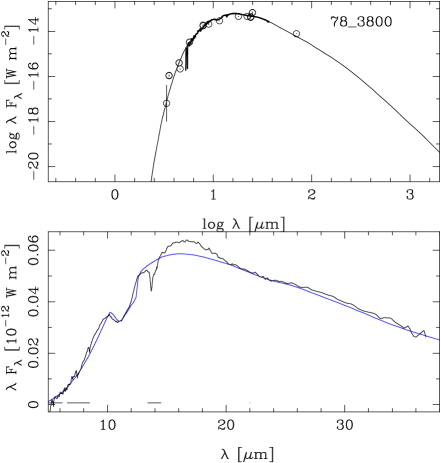
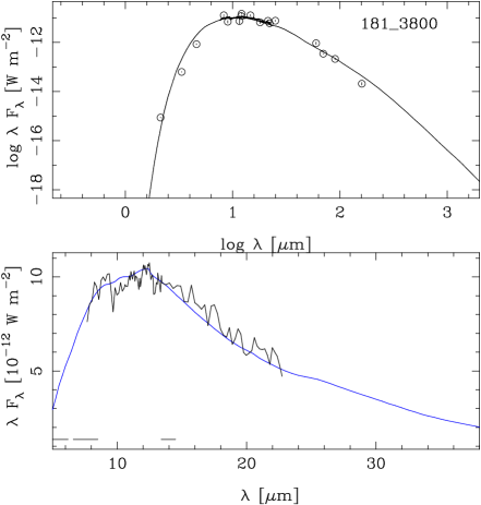
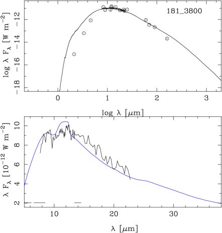
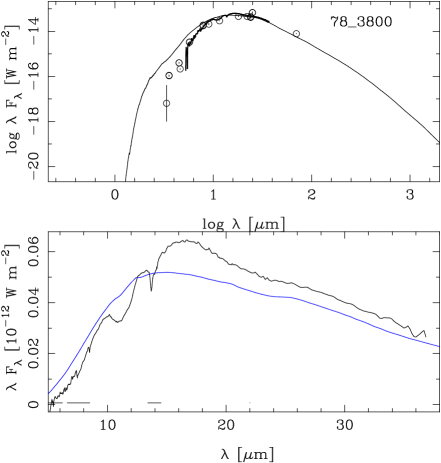
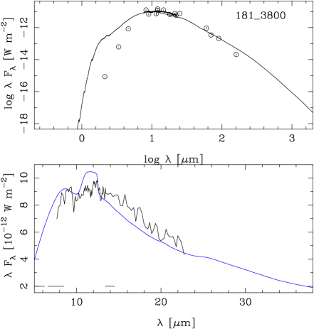
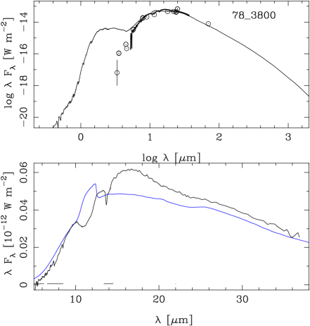
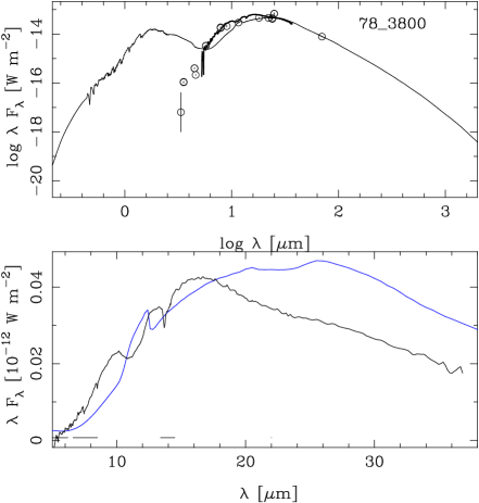
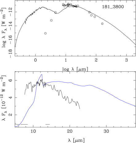
Figure 22: Same as for figure 6, but when the effective temperature of the central star is 3800 K.

Appendix E Comparison to ZTF

The referee pointed out the paper of Chen et al. (2020), who classified about 780 000 periodic variables into 11 classes using ZTF datarelease 2 data. The sample of 1992 objects was correlated with this database using a search radius of 1″. Sixty-three matches were found, with 50 stars being classified as Miras and 12 as semi-regulars by Chen et al. (2020). Table LABEL:AppTabZTF compiles the periods found from WISE and our analysis of the ZTF data, as well as the periods found by Chen et al. (2020). We note that periods found in the literature or from refitting other datasets in the present paper are not repeated in the Table.

The periods found by Chen et al. (2020) compare rather poorly to the periods derived in the present paper from WISE data or ZTF data. Only for 20 do the periods agree within 10 percent. For many, the periods derived in the present paper are longer, sometimes by a factor of 2. The reason is that the ZTF data only cover a time span of 470 days, and so, citing Chen et al. (2020), ‘the periods in our catalogue are most accurate for P $<$ 100 days. This limitation causes problems for the periods of SRs and Miras’. The advantage of the manual fitting and visual inspection, as was done in the present paper for the external data, is that periods longer than the time span of the dataset can be assigned with confidence.

7]

Table 10: Comparison with Chen et al. (2020).

Ra	Dec	$P_{1}$	$P_{2}$	$P_{\rm ZTF}$	ZTF Id	Period	ZTF class
(deg)	(deg)	(d)	(d)	(d)		(d)
5.193017	64.514450	549	270	519 $\pm$ 30	ZTFJ002046.32+643051.9	284	SR
6.921023	69.647507			637 $\pm$ 55	ZTFJ002741.12+693851.5	425	Mira
23.869953	49.378334			491 $\pm$ 11	ZTFJ013528.77+492242.0	440	Mira
62.743782	52.385670	920	928		ZTFJ041058.47+522308.2	282	SR
64.966774	51.740726	463	477	445 $\pm$ 34	ZTFJ041952.04+514426.4	400	Mira
65.558540	59.980003	573		511 $\pm$ 19	ZTFJ042214.10+595848.0	440	Mira
66.168434	48.123432				ZTFJ042440.46+480724.0	794	Mira
70.127876	45.125114	538	565	517 $\pm$ 5	ZTFJ044030.68+450730.3	603	Mira
71.838844	39.451748	512	482	428 $\pm$ 71	ZTFJ044721.35+392706.2	540	Mira
78.351913	20.990301				ZTFJ051324.44+205924.9	454	Mira
81.536049	47.125359	585	466	480 $\pm$ 7	ZTFJ052608.61+470731.2	295	Mira
85.957069	32.701687			606 $\pm$ 85	ZTFJ054349.66+324206.5	487	Mira
86.118340	42.851227			326 $\pm$ 4	ZTFJ054428.38+425104.2	443	Mira
90.742348	46.461830	453	430	406 $\pm$ 21	ZTFJ060258.13+462742.4	374	Mira
97.397789	8.788045			769 $\pm$ 75	ZTFJ062935.45+084716.5	483	Mira
97.832855	31.528938	537	559	666 $\pm$ 18	ZTFJ063119.87+313144.0	521	Mira
98.616814	-5.061915			$-$	ZTFJ063428.06-050343.0	171	SR
101.275536	-8.471849	638	671	558 $\pm$ 13	ZTFJ064506.11-082818.8	363	Mira
101.500809	15.663664			552 $\pm$ 10	ZTFJ064600.17+153948.9	385	Mira
103.519295	-4.326680			377 $\pm$ 8	ZTFJ065404.65-041936.3	187	SR
104.773621	3.632370	564	550	424 $\pm$ 9	ZTFJ065905.66+033756.2	181	SR
107.645561	-1.190360	627	675	539 $\pm$ 11	ZTFJ071034.93-011125.5	406	Mira
107.780273	-0.386771	623	577		ZTFJ071107.28-002312.6	318	SR
110.524391	-3.546792	399	362	380 $\pm$ 6	ZTFJ072205.85-033248.4	367	SR
114.012138	-10.214721				ZTFJ073602.90-101253.1	480	Mira
274.574738	-10.595833	602	553	402 $\pm$ 9	ZTFJ181817.92-103545.0	457	Mira
280.056274	-5.703139			557 $\pm$ 10	ZTFJ184013.49-054211.4	540	Mira
282.231476	-1.815691	429	432	397 $\pm$ 2	ZTFJ184855.50-014856.9	394	Mira
282.813995	1.652694	524	480		ZTFJ185115.41+013909.6	451	Mira
283.761780	15.786965	450	447	458 $\pm$ 6	ZTFJ185502.79+154713.2	445	Mira
285.819824	9.203329	496	468		ZTFJ190316.78+091211.9	216	SR
287.820007	17.864273	445	422	422 $\pm$ 3	ZTFJ191116.77+175150.7	440	Mira
288.179382	5.886957			$-$	ZTFJ191243.03+055312.9	169	SR
288.304840	12.003804	446	430	417 $\pm$ 12	ZTFJ191313.18+120013.7	375	Mira
289.141144	18.381018	437	417	407 $\pm$ 5	ZTFJ191633.90+182251.8	409	Mira
291.094452	32.319031	560	540	520 $\pm$ 211	ZTFJ192422.61+321908.4	578	Mira
291.536896	23.480146	586	570	681 $\pm$ 25	ZTFJ192608.79+232848.3	215	SR
291.658112	18.266577	520	590	490 $\pm$ 15	ZTFJ192637.94+181559.0	500	Mira
291.916656	23.792528	612	589	455 $\pm$ 9	ZTFJ192739.97+234732.3	517	Mira
292.580017	17.180479	694	651		ZTFJ193019.22+171049.8	373	SR
293.548218	19.974556	441	427	421 $\pm$ 16	ZTFJ193411.56+195828.1	427	Mira
294.350159	20.616007	521	494	358 $\pm$ 12	ZTFJ193723.99+203657.7	436	Mira
295.230194	15.337878	550	533	493 $\pm$ 19	ZTFJ194055.25+152015.9	408	Mira
295.535187	47.382542	460	453	394 $\pm$ 6	ZTFJ194208.42+472257.0	304	Mira
296.269775	6.959763	455	408	399 $\pm$ 6	ZTFJ194504.72+065735.4	385	Mira
297.452881	35.820549	453	445	491 $\pm$ 7	ZTFJ194948.67+354913.8	447	Mira
297.872650	27.149763	906	873	793 $\pm$ 122	ZTFJ195129.43+270858.8	350	Mira
298.620667	24.372654			597 $\pm$ 37	ZTFJ195428.94+242221.5	527	Mira
299.963959	32.536037			408 $\pm$ 4	ZTFJ195951.33+323209.8	408	Mira
302.033997	31.716911			468 $\pm$ 7	ZTFJ200808.16+314300.9	422	Mira
305.475128	36.560566			$-$	ZTFJ202154.04+363338.0	556	Mira
309.914825	50.204674	462	502	442 $\pm$ 2	ZTFJ203939.51+501216.4	457	Mira
315.385437	38.756172	517	607	462 $\pm$ 4	ZTFJ210132.52+384522.3	523	Mira
315.992218	50.244583	2411	1523	321 $\pm$ 3	ZTFJ210358.11+501440.2	318	SR
317.444366	18.413706	368	371	445 $\pm$ 6	ZTFJ210946.62+182449.2	425	Mira
317.659851	45.979378	542	548	442 $\pm$ 2	ZTFJ211038.36+455845.9	424	Mira
319.133759	36.358849	476	541	624 $\pm$ 20	ZTFJ211632.10+362132.0	460	Mira
325.987213	58.596138	506	503	596 $\pm$ 48	ZTFJ214356.93+583546.1	480	Mira
334.659912	43.778919			$-$	ZTFJ221838.38+434644.5	580	Mira
339.322784	59.454674	590	587	519 $\pm$ 28	ZTFJ223717.44+592717.0	613	Mira
352.573853	53.883614	506	553	573 $\pm$ 46	ZTFJ233017.75+535301.1	520	Mira
353.614540	43.550311			686 $\pm$ 21	ZTFJ233427.48+433300.8	510	Mira
357.904877	63.010296	611	626	558 $\pm$ 20	ZTFJ235137.16+630036.9	292	SR