Bottom-Up Reconstruction of Viable GW170817 Compatible Einstein-Gauss-Bonnet Theories

Abstract

In this work we shall use a bottom-up approach for obtaining viable inflationary Einstein-Gauss-Bonnet models which are also compatible with the GW170817 event. Specifically, we shall use a recently developed theoretical framework in which we shall specify only the tensor-to-scalar ratio, in terms of the $e$-foldings number. Starting from the tensor-to-scalar ratio, we shall reconstruct from it the Einstein-Gauss-Bonnet theory which can yield such a tensor-to-scalar ratio, finding the scalar potential and the Gauss-Bonnet coupling scalar function as functions of the $e$-foldings number. Accordingly, the calculation of the spectral index of the primordial scalar perturbations, and of the tensor spectral index easily is greatly simplified and these observational indices can easily be found. After presenting the general formalism for the bottom-up reconstruction, we exemplify our findings by presenting several Einstein-Gauss-Bonnet models of interest which yield a viable inflationary phenomenology. These models have also an interesting common characteristic, which is a blue tilted tensor spectral index. We also investigate the predicted energy spectrum of the primordial gravitational waves for these Einstein-Gauss-Bonnet models, and as we show, all the models yield a detectable primordial wave energy power spectrum.

I Introduction

In the next two decades, the cosmologists’s community anticipates a great amount of information coming from the sky. This information will either validate the current state of art thinking on cosmological issues, or will exclude current theories and thus our perception about the early Universe will utterly change. Indeed, in about 10-15 years from now, several experiments that are based on astronomical observations will commence to yield their first data, like for example LISA Baker:2019nia ; Smith:2019wny . But also several other future proposed experiments might also begin to operate, like BBO Crowder:2005nr ; Smith:2016jqs and DECIGO Seto:2001qf ; Kawamura:2020pcg . During the 2010’s decade, the cosmological community has already experienced the first surprises coming from the sky. Specifically, the GW170817 kilonova accompanied event TheLIGOScientific:2017qsa ; Monitor:2017mdv ; GBM:2017lvd , imposed severe constraints to theories that predict tensor spacetime perturbations with gravitational wave speed $c_{T}^{2}$ different from unity in natural units. Specifically, the electromagnetic counterpart to GW170817 indicates that the deviation in the speed of gravitational waves from that of light must roughly be $|c_{T}/c-1|\leq 5\times 10^{-16}$, see for example Refs. Ezquiaga:2017ekz ; Baker:2017hug ; Creminelli:2017sry ; Sakstein:2017xjx ; Fernandes:2022zrq . One relevant example in which case the theory predicts $c_{T}^{2}\neq 1$, while comfortably well fitted within observational constraints, are the scalar-tensor formulations of four-dimensional Einstein-Gauss-Bonnet gravity, see for example the recent review Fernandes:2022zrq . In these models, the GW170817 event imposes only mild constraints on the coupling constant of the theory. For more details on the constraints imposed by the GW170817 event on several versions of modified gravity and scalar tensor gravity, see for example Ezquiaga:2017ekz ; Baker:2017hug ; Creminelli:2017sry ; Sakstein:2017xjx ; Fernandes:2022zrq . In recent works Odintsov:2020sqy ; Oikonomou:2021kql we provided a theoretical framework for Einstein-Gauss-Bonnet theories Hwang:2005hb ; Nojiri:2006je ; Cognola:2006sp ; Nojiri:2005vv ; Nojiri:2005jg ; Satoh:2007gn ; Bamba:2014zoa ; Yi:2018gse ; Guo:2009uk ; Guo:2010jr ; Jiang:2013gza ; Kanti:2015pda ; vandeBruck:2017voa ; Kanti:1998jd ; Dominguez:2005rt ; Maeda:2005ci ; Ghosh:2011ad ; Maharaj:2015gsd ; Brassel:2019bam ; Pozdeeva:2020apf ; Vernov:2021hxo ; Pozdeeva:2021iwc ; Koh:2014bka ; Bayarsaikhan:2020jww ; Tumurtushaa:2018lnv ; Fomin:2020hfh ; DeLaurentis:2015fea ; Chervon:2019sey ; Nozari:2017rta ; Odintsov:2018zhw ; Kawai:1998ab ; Yi:2018dhl ; vandeBruck:2016xvt ; Kleihaus:2019rbg ; Bakopoulos:2019tvc ; Maeda:2011zn ; Bakopoulos:2020dfg ; Ai:2020peo ; Oikonomou:2020oil ; Odintsov:2020xji ; Oikonomou:2020sij ; Odintsov:2020zkl ; Odintsov:2020mkz ; Venikoudis:2021irr ; Kong:2021qiu ; Easther:1996yd ; Antoniadis:1993jc ; Antoniadis:1990uu ; Kanti:1995vq ; Kanti:1997br which yields GW170817-compatible models with gravitational wave speed $c_{T}^{2}\simeq 1$ in natural units, thus equal to that of light’s. Einstein-Gauss-Bonnet theories are interesting on their own, since these are generalizations of the Einstein-Hilbert action, which contains linear forms of curvature. In contrast, Einstein-Gauss-Bonnet theories contain more than just linear forms of the Riemann tensor, the Ricci tensor and the Ricci scalar. Basically, Einstein-Gauss-Bonnet gravity is a specific case of Lovelock gravity Lovelock:1971yv ; Lovelock:1972vz . Lovelock gravity applies to higher order and higher dimensional theories of gravity, and Einstein-Gauss-Bonnet gravity is the second-order limiting case of general Lovelock’s theory while Einstein’s general relativity, is the first-order Lovelock theory. It is a well known fact that Einstein-Gauss-Bonnet gravity has a minimum dimension of five, whereas general relativity has a minimum dimension of four. So effectively Einstein-Gauss-Bonnet gravity has a general relativity limit but only in five dimensions.

In this work we aim to provide a bottom-up reconstruction technique for viable Einstein-Gauss-Bonnet theories developed in Oikonomou:2021kql . We shall use the theoretical framework developed in Oikonomou:2021kql , and starting from the tensor-to-scalar ratio given as a desired function of the $e$-foldings number, we shall reconstruct the Einstein-Gauss-Bonnet theory which can yield such a tensor-to-scalar ratio. Specifically, we shall find the scalar potential and the Gauss-Bonnet scalar coupling function, as functions of the $e$-foldings number. From these, the calculation of the scalar and tensor spectral indices easily follows, and thus the whole framework is available for checking the viability of several Einstein-Gauss-Bonnet models. We shall exemplify the techniques of the bottom-up reconstruction formalism, by presenting several viable inflationary Einstein-Gauss-Bonnet models. Also, due to the fact that these models result to a positive tensor spectral index, we shall also calculate the predicted primordial gravitational wave energy spectrum for each of these models. As we show, these models can yield a detectable signal of primordial gravitational waves. Another interesting feature of the models which we shall present is the fact that some of the models can yield a small tensor-to-scalar ratio, which can be useful in the future, if the stage 4 Cosmic Microwave Background experiments further constraint the tensor-to-scalar ratio to smaller values.

This paper is organized as follows: In section II we overview in brief the theoretical framework of GW170817-compatible Einstein-Gauss-Bonnet theories developed in Oikonomou:2021kql . In section III we present our bottom-up reconstruction approach in order to study phenomenologically viable Einstein-Gauss-Bonnet theories. In section IV we present several illustrative examples of viable Einstein-Gauss-Bonnet models using our bottom up reconstruction techniques, and we also present the potential ability of these model to generate a detectable energy spectrum of primordial gravitational waves. Finally, the conclusions follow at the end of the paper.

II Brief Overview of GW170817-Compatible Einstein-Gauss-Bonnet Theories

In this section we shall briefly review the reformed GW170817-compatible formalism for Einstein-Gauss-Bonnet theories developed in Ref. Oikonomou:2021kql . The vacuum Einstein-Gauss-Bonnet gravity action has the following form,

$$\centering S=\int{d^{4}x\sqrt{-g}\left(\frac{R}{2\kappa^{2}}-\frac{1}{2}\partial_{\mu}\phi\partial^{\mu}\phi-V(\phi)-\frac{1}{2}\xi(\phi)\mathcal{G}\right)}\,,\@add@centering$$ (1)

with $R$ denoting the Ricci scalar, $\kappa=\frac{1}{M_{p}}$ with $M_{p}$ being the reduced Planck mass. Moreover, $\mathcal{G}$ denotes the Gauss-Bonnet invariant in dimension-4, which is $\mathcal{G}=R^{2}-4R_{\alpha\beta}R^{\alpha\beta}+R_{\alpha\beta\gamma\delta}R^{\alpha\beta\gamma\delta}$ where $R_{\alpha\beta}$ and $R_{\alpha\beta\gamma\delta}$ denote the Ricci and Riemann tensor respectively. Also for the rest of this paper we shall assume that the geometry of spacetime is described by a flat Friedmann-Robertson-Walker (FRW) metric, with line element,

$$\centering ds^{2}=-dt^{2}+a(t)^{2}\sum_{i=1}^{3}{(dx^{i})^{2}}\,,\@add@centering$$ (2)

where $a$ denotes the scale factor and also for the FRW metric, the Gauss-Bonnet invariant takes the form $\mathcal{G}=24H^{2}(\dot{H}+H^{2})$. Furthermore, we shall assume that the scalar field is solely time-dependent. The field equations are easily derived by varying the gravitational action with respect to the metric and to the scalar field, and these are,

$$\centering\frac{3H^{2}}{\kappa^{2}}=\frac{1}{2}\dot{\phi}^{2}+V+12\dot{\xi}H^{3}\,,\@add@centering$$ (3)

$$\centering\frac{2\dot{H}}{\kappa^{2}}=-\dot{\phi}^{2}+4\ddot{\xi}H^{2}+8\dot{\xi}H\dot{H}-4\dot{\xi}H^{3}\,,\@add@centering$$ (4)

$$\centering\ddot{\phi}+3H\dot{\phi}+V^{\prime}+12\xi^{\prime}H^{2}(\dot{H}+H^{2})=0\,,\@add@centering$$ (5)

where the “dot” denotes differentiations with respect to the cosmic time $t$. Following Ref. Oikonomou:2021kql , by imposing the slow-roll conditions,

$$\dot{H}\ll H^{2},\,\,\ \frac{\dot{\phi}^{2}}{2}\ll V,\,\,\,\ddot{\phi}\ll 3H\dot{\phi}\,.$$ (6)

and also the constraint $c_{T}^{2}=1$, where $c_{T}^{2}$ is,

$$\centering c_{T}^{2}=1-\frac{Q_{f}}{2Q_{t}}\,,\@add@centering$$ (7)

and $Q_{f}$, $Q_{b}$ appearing above are $Q_{f}=8(\ddot{\xi}-H\dot{\xi})$, $Q_{t}=F+\frac{Q_{b}}{2}$, where $F$ is equal to $F=\frac{1}{\kappa^{2}}$ while $Q_{b}=-8\dot{\xi}H$, the field equations are simplified as follows,

$$\centering H^{2}\simeq\frac{\kappa^{2}V}{3}\,,\@add@centering$$ (8)

$$\centering\dot{H}\simeq-\frac{1}{2}\kappa^{2}\dot{\phi}^{2}\,,\@add@centering$$ (9)

$$\centering\dot{\phi}\simeq\frac{H\xi^{\prime}}{\xi^{\prime\prime}}\,.\@add@centering$$ (10)

Moreover, the scalar potential and the Gauss-Bonnet scalar coupling function must satisfy the following constraint differential equation,

$$\centering\frac{V^{\prime}}{V^{2}}+\frac{4\kappa^{4}}{3}\xi^{\prime}\simeq 0\,.\@add@centering$$ (11)

The slow-roll indices for Einstein-Gauss-Bonnet models are Hwang:2005hb ,

$$\epsilon_{1}=-\frac{\dot{H}}{H^{2}},\,\,\,\epsilon_{2}=\frac{\ddot{\phi}}{H\dot{\phi}},\,\,\,\epsilon_{4}=\frac{\dot{E}}{2HE},$$ (12)

$$\epsilon_{5}=\frac{Q_{a}}{2HQ_{t}},\,\,\,\epsilon_{6}=\frac{\dot{Q}_{t}}{2HQ_{t}}\,,$$

with $E$ is defined as follows,

$$E=\frac{F}{\dot{\phi}^{2}}\left(\dot{\phi}^{2}+3\left(\frac{Q_{a}^{2}}{2Q_{t}}\right)\right)\,,$$ (13)

where $Q_{a}$, for the Einstein-Gauss-Bonnet theory is Hwang:2005hb ,

$$Q_{a}=-4\dot{\xi}H^{2}\,.$$ (14)

Employing the simplified equations of motion (8)- (10), the slow-roll indices finally become,

$$\centering\epsilon_{1}\simeq\frac{\kappa^{2}}{2}\left(\frac{\xi^{\prime}}{\xi^{\prime\prime}}\right)^{2}\,,\@add@centering$$ (15)

$$\centering\epsilon_{2}\simeq 1-\epsilon_{1}-\frac{\xi^{\prime}\xi^{\prime\prime\prime}}{\xi^{\prime\prime 2}}\,,\@add@centering$$ (16)

$$\centering\epsilon_{4}\simeq\frac{\xi^{\prime}}{2\xi^{\prime\prime}}\frac{\mathcal{E}^{\prime}}{\mathcal{E}}\,,\@add@centering$$ (17)

$$\centering\epsilon_{5}\simeq-\frac{\epsilon_{1}}{\lambda}\,,\@add@centering$$ (18)

$$\centering\epsilon_{6}\simeq\epsilon_{5}(1-\epsilon_{1})\,,\@add@centering$$ (19)

with, $\mathcal{E}=\mathcal{E}(\phi)$ and $\lambda=\lambda(\phi)$ being defined as follows,

$$\mathcal{E}(\phi)=\frac{1}{\kappa^{2}}\left(1+72\frac{\epsilon_{1}^{2}}{\lambda^{2}}\right),\,\,\,\lambda(\phi)=\frac{3}{4\xi^{\prime\prime}\kappa^{2}V}\,.$$ (20)

Regarding the observational indices, we have Hwang:2005hb ,

$$\centering n_{\mathcal{S}}=1-4\epsilon_{1}-2\epsilon_{2}-2\epsilon_{4}\,,\@add@centering$$ (21)

for the spectral index of the primordial scalar perturbations, while the tensor spectral index is Oikonomou:2021kql ,

$$n_{\mathcal{T}}\simeq-2\epsilon_{1}\left(1-\frac{1}{\lambda}+\frac{\epsilon_{1}}{\lambda}\right)\,.$$ (22)

Finally, the tensor-to-scalar ratio is,

$$r\simeq 16\epsilon_{1}\,.$$ (23)

In the next section, we shall use the equations and expressions of this section, in order to employ and introduce the bottom-up reconstruction method for Einstein-Gauss-Bonnet theories.

III Reconstruction of Inflationary Phenomenology from the Observational Indices: A Bottom-up Approach

For our general solution it is essential to express every variable as a function of $N$, which is the number of $e$-foldings. To achieve that we write,

$$\centering\xi^{\prime}(\phi)=\frac{dN}{d\phi}\frac{d\xi}{dN},\@add@centering$$ (24)

and

$$\xi^{\prime\prime}=\frac{d\xi^{\prime}}{d\phi}=\frac{dN}{d\phi}\frac{d}{dN}\left(\frac{dN}{d\phi}\frac{d\xi}{dN}\right)=\left(\frac{dN}{d\phi}\right)^{2}\frac{d^{2}\xi}{dN^{2}}+\xi^{\prime}\frac{d}{dN}\left(\frac{dN}{d\phi}\right),$$ (25)

where the “prime”, denotes differentiation with respect to the scalar field. Using Eq. (15), (23) and

$$\centering\frac{\xi^{\prime\prime}}{\xi^{\prime}}=\frac{dN}{d\phi},\@add@centering$$ (26)

which follows from Eq. (24) we obtain,

$$\centering r(N)=8\kappa^{2}\left(\frac{d\phi}{dN}\right)^{2},\@add@centering$$ (27)

which is the general form of the tensor-to-scalar ratio as a function of the number of $e$-foldings, in the Einstein-Gauss-Bonnet theory. The previous expression can be written as,

$$\centering\frac{dN}{d\phi}=\frac{2\kappa\sqrt{2}}{\sqrt{r}},\@add@centering$$ (28)

and thus we obtain a useful expression for $\xi^{\prime}$ and $\xi^{\prime\prime}$

$$\centering\xi^{\prime}=\frac{dN}{d\phi}\frac{d\xi}{dN}=\frac{2\kappa\sqrt{2}}{\sqrt{r}}\frac{d\xi}{dN},\@add@centering$$ (29)

$$\xi^{\prime\prime}=\frac{8\kappa^{2}}{r}\frac{d^{2}\xi}{dN^{2}}-\frac{4\kappa^{2}}{r^{2}}\frac{dr}{dN}\frac{d\xi}{dN}.$$ (30)

Using the previous equations and the fact that $\xi^{\prime\prime}=\frac{dN}{d\phi}\xi^{\prime}$ we have,

$$\xi^{\prime\prime}=\frac{8\kappa^{2}}{r}\frac{d^{2}\xi}{dN^{2}}-\frac{4\kappa^{2}}{r^{2}}\frac{dr}{dN}\frac{d\xi}{dN}=\frac{2\kappa\sqrt{2}}{\sqrt{r}}\frac{2\kappa\sqrt{2}}{\sqrt{r}}\frac{d\xi}{dN}=\frac{8\kappa^{2}}{r}\frac{d\xi}{dN}.$$ (31)

From Eq. (31) we derive the differential equation of the coupling function with respect to the number of $e$-foldings,

$$\centering\frac{d^{2}\xi}{dN^{2}}-\left(\frac{1}{2r}\frac{dr}{dN}+1\right)\frac{d\xi}{dN}=0,\@add@centering$$ (32)

and its solution is,

$$\centering\xi(N)=C_{1}\int\sqrt{r(N)}e^{N}dN+C_{2},\@add@centering$$ (33)

where $C_{1}$, $C_{2}$ are two arbitrary integration constants. From Eq. (11), the potential of the scalar field takes the following form,

$$\frac{1}{V^{2}}\frac{dV}{d\phi}+\frac{4\kappa^{4}}{3}\frac{d\xi}{d\phi}=0.$$ (34)

Combining Eqs. (34), (24) we get,

$$\frac{1}{V^{2}}\frac{dN}{d\phi}\frac{dV}{dN}+\frac{4\kappa^{4}}{3}\frac{dN}{d\phi}\frac{d\xi}{dN}=0.$$ (35)

Eq. (35) is a differential equation satisfied by the potential of the scalar field with respect to the number of $e$-foldings, $N$. Its general solution is,

$$\centering V(N)=\frac{3}{4\kappa^{4}}\frac{1}{\xi(N)}.\@add@centering$$ (36)

Thus employing this bottom-up reconstruction method we just presented, we are able to derive the scalar coupling function, the potential of the scalar field and the spectral indices $n_{\mathcal{S}}$, $n_{T}$ for various expressions of the tensor-to-scalar ratio as a function of the number of $e$-foldings. In the next section we shall present several illustrative examples of viable Einstein-Gauss-Bonnet inflationary models, which are derived by employing our bottom-up reconstruction approach.

IV Application of the Bottom-up Formalism: Phenomenology of Various Models

We proceed by exploring the phenomenology of different models, using the method we developed in the previous section. For most of our models we shall choose a tensor-to-scalar ratio of the form $r=\delta/N^{d}$ where $d>0$. By varying the parameter $\delta$, so that the tensor-to-scalar ratio is within the Planck 2018 Planck:2018jri constraints $r<0.056$, we solved the equation $n_{\mathcal{S}}(C_{1})=0.9649\pm 0.0042$ for $C_{2}=1$. For each set of the parameters $\delta$, and $n_{\mathcal{S}}$ there are three different values for the parameter $C_{1}$, which verify the equation and each of these gives a different $n_{T}$: a negative one (about -0.04) and two positive (about 0.04 and 0.92) ones. In all the cases for which $r=\delta/N^{d}$, the parameter $C_{1}$ turns out to be $C_{1}\mathcal{O}(10^{-27}-10^{-24})$ in order for the models to be rendered viable. The last of our models is an exponential model of the form of $r=ae^{-bN}$. The methodology is the same with the previous models, only here the free parameters of the model are $a$ and $b$. In our study the value of the integration constant $C_{2}$ did not affect any of the calculated indices, and so we kept $C_{2}=1$ in every model. For brevity we will not show the evaluation of the slow-roll indices and the analytical expression of the scalar spectral index $n\mathrm{S}$, since these are too lengthy.

IV.1 Model I: The Case with $r=\delta/N$

We start with the simplest possible model of our study, in which case,

$$\centering r=\frac{\delta}{N}.\@add@centering$$ (37)

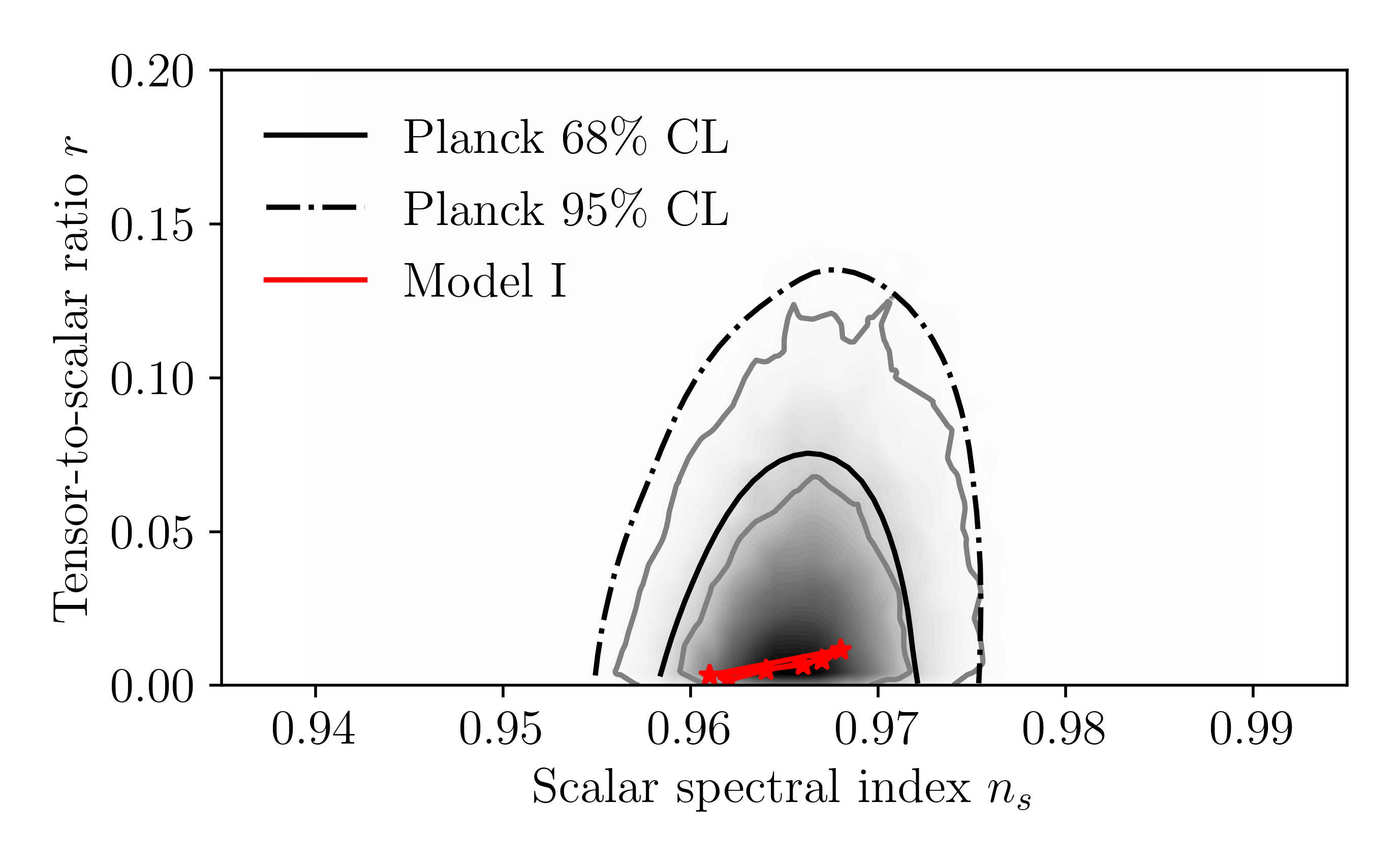
Figure 1: Planck 2018 Likelihood Curves for the Model I with $r=\delta/N$ model

From Eq. (33) it follows that the scalar coupling function $\xi$ takes the form,

$$\centering\xi=2C_{1}\sqrt{\delta}e^{N}\operatorname{D}(\sqrt{N})+C_{2},\@add@centering$$ (38)

where $\operatorname{D}(x)$ is the Dawson integral, defined as $\operatorname{D}(x)=e^{-x^{2}}\int_{0}^{x}e^{t^{2}}dt$. From Eq. (36) it follows that the potential of the scalar field $V$ takes the form,

$$\centering V(N)=\frac{3}{4\kappa^{4}\left(2C_{1}e^{N}\sqrt{\delta}\operatorname{D}\left(\sqrt{N}\right)+C_{2}\right)},\@add@centering$$ (39)

To calculate the scalar spectral index, the corresponding value of the tensor-to-scalar ratio and the tensor spectral index, we need to calculate the slow-roll indices. To do that we use the function $\lambda(N)$ (20), which for this model is,

$$\centering\lambda(N)=\frac{C_{2}}{8C_{1}}\sqrt{\frac{\delta}{N}}e^{-N}+\frac{\delta\operatorname{D}(\sqrt{N})}{4\sqrt{N}}.\@add@centering$$ (40)

Using Eq. (22) the tensor spectral index takes the form,

$$\centering n_{T}=-\frac{2C_{2}\delta\sqrt{N}+C_{1}\sqrt{\delta}e^{N}\left(\delta-16N4\delta\sqrt{N}\operatorname{D}(\sqrt{N})\right)}{16C_{2}N^{\frac{3}{2}}+32C_{1}\sqrt{\delta}e^{N}N^{\frac{3}{2}}\operatorname{D}(\sqrt{N})}.\@add@centering$$ (41)

The upper limit of the $\delta$ parameter, in order for the tensor-to-scalar ratio $r$ to comply with $2018$ Planck constrains, is $3.36$. By varying the parameter $\delta$, $n_{\mathcal{S}}$, $C_{1}$ and $C_{2}$ with respect to the Planck constraints we evaluated the tensor-to-scalar ratio and the tensor spectral index. In the Table 1 we present a small portion of the set of values of the observational indices we calculated.

Table 1: Different values for $\delta$ and $n_{\mathcal{S}}$ and the corresponding $n_{T}$ and $r$ for Model I

$\delta$	$r$	$n_{\mathcal{S}}$	$n_{T}$
0.001	$1.66667\cdot 10^{-5}$	0.965	0.964288
0.05	0.000833333	0.965	0.964191
0.1	0.00166667	0.965	0.039063
1	0.016667	0.961	0.037994
3	0.05	0.969	0.960455

Using the data presented in the Table 1 we confront the model with the Planck 2018 data Planck:2018jri , and the results are presented in Fig. 1. As it can be seen in Fig. 1, Model I is well fitted deeply in the Planck likelihood curves. Also in Fig. 2

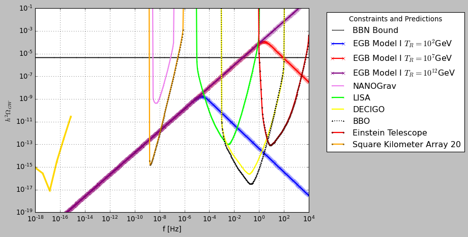
Figure 2: The $h^{2}$-scaled primordial gravitational waves energy spectrum for the Model I, versus the sensitivity curves of future primordial gravitational waves experiments.

we plot the $h^{2}$-scaled primordial gravitational waves energy spectrum for the Model I, versus the sensitivity curves of future primordial gravitational waves experiments for three reheating temperatures. We chose the smallest value of the predicted tensor-to-scalar ratio and the corresponding blue-tilted spectral index. As it can be seen, the predicted energy spectrum lies within the reach of future experiments.

IV.2 Model II: The Case with $r=\delta/N^{2}$

The next model we shall consider has the following tensor-to-scalar ratio,

$$\centering r=\frac{\delta}{N^{2}}.\@add@centering$$ (42)

Again we calculate $\xi$ from Eq. (33),

$$\centering\xi=2C_{1}\sqrt{\delta}\operatorname{Ei}(N)+C_{2},\@add@centering$$ (43)

where $\operatorname{Ei}(x)$ is the Exponential integral, defined as $\operatorname{Ei}(x)=\int_{-\infty}^{x}\frac{e^{t}}{t}dt$

Figure 3: Planck 2018 Likelihood Curves for the Model II for $r=\delta/N^{2}$.

We proceed to the calculation of the potential of the scalar field $V$ by applying Eq. (36),

$$\centering V(N)=\frac{3}{4\kappa^{4}\left(2C_{1}\sqrt{\delta}\operatorname{Ei}(N)+C_{2}\right)},\@add@centering$$ (44)

and he function $\lambda(N)$ is,

$$\centering\lambda(N)=\frac{C_{2}\sqrt{\delta}}{8C_{1}}\frac{e^{-N}}{N}+\frac{\delta}{8}\frac{e^{-N}\operatorname{Ei}(N)}{N}.\@add@centering$$ (45)

From Eq. (22) it follows that the tensor spectral index $n_{T}$ takes the form,

$$\centering n_{T}=-\frac{\sqrt{\delta}\left(2C_{2}\sqrt{\delta}N+C_{1}e^{N}\left(\delta-16N^{2}\right)+2C_{1}\delta N\operatorname{Ei}(N)\right)}{16N^{3}\left(C_{2}+C_{1}\sqrt{\delta}\operatorname{Ei}(N)\right)}.\@add@centering$$ (46)

The upper limit of the $\delta$ parameter, in order for the tensor-to-scalar ratio $r$ to comply with $2018$ Planck constraints, is $201.6$. In Table 2 we present some of the values of the observational indices we calculated.

Table 2: Different values for $\delta$ and $n_{\mathcal{S}}$ and the corresponding $n_{T}$ and $r$ for Model II

$\delta$	$r$	$n_{\mathcal{S}}$	$n_{T}$
1	0.000277778	0.961	0.944884
5	0.00138889	0.962	0.945287
10	0.00277778	0.964	0.946191
15	0.00416667	0.967	0.947627
20	0.00555556	0.968	0.947996

Using the data presented in Table 2 we confront the model with the Planck 2018 data Planck:2018jri , and the results are presented in Fig. 3. As it can be seen in Fig. 3, Model II is well fitted deeply in the Planck likelihood curves, as in the previous model. Also in Fig. 4

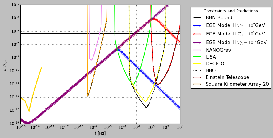
Figure 4: The $h^{2}$-scaled primordial gravitational waves energy spectrum for the Model II, versus the sensitivity curves of future primordial gravitational waves experiments.

we plot the $h^{2}$-scaled primordial gravitational waves energy spectrum for the Model II, versus the sensitivity curves of future primordial gravitational waves experiments for three reheating temperatures. In this case too we chose the smallest value of the predicted tensor-to-scalar ratio and the corresponding blue-tilted spectral index. As in the previous case, the predicted energy spectrum lies within the reach of future experiments.

IV.3 Model III: The case with $r=\delta/N^{3}$

In this model the expression of the tensor-to-scalar ratio is,

$$\centering r=\frac{\delta}{N^{3}}.\@add@centering$$ (47)

The scalar coupling function of this model $\xi(N)$ is,

$$\centering\xi(N)=C_{2}-2C_{1}\sqrt{\frac{\delta}{N^{3}}}N\left(e^{N}+N\operatorname{E}_{\frac{1}{2}}(-N)\right),\@add@centering$$ (48)

where $\operatorname{E}_{n}(x)$ is the Exponential integral function, defined as $\operatorname{E}_{n}(x)=\int_{1}^{\infty}\frac{e^{-xt}}{t^{n}}dt$

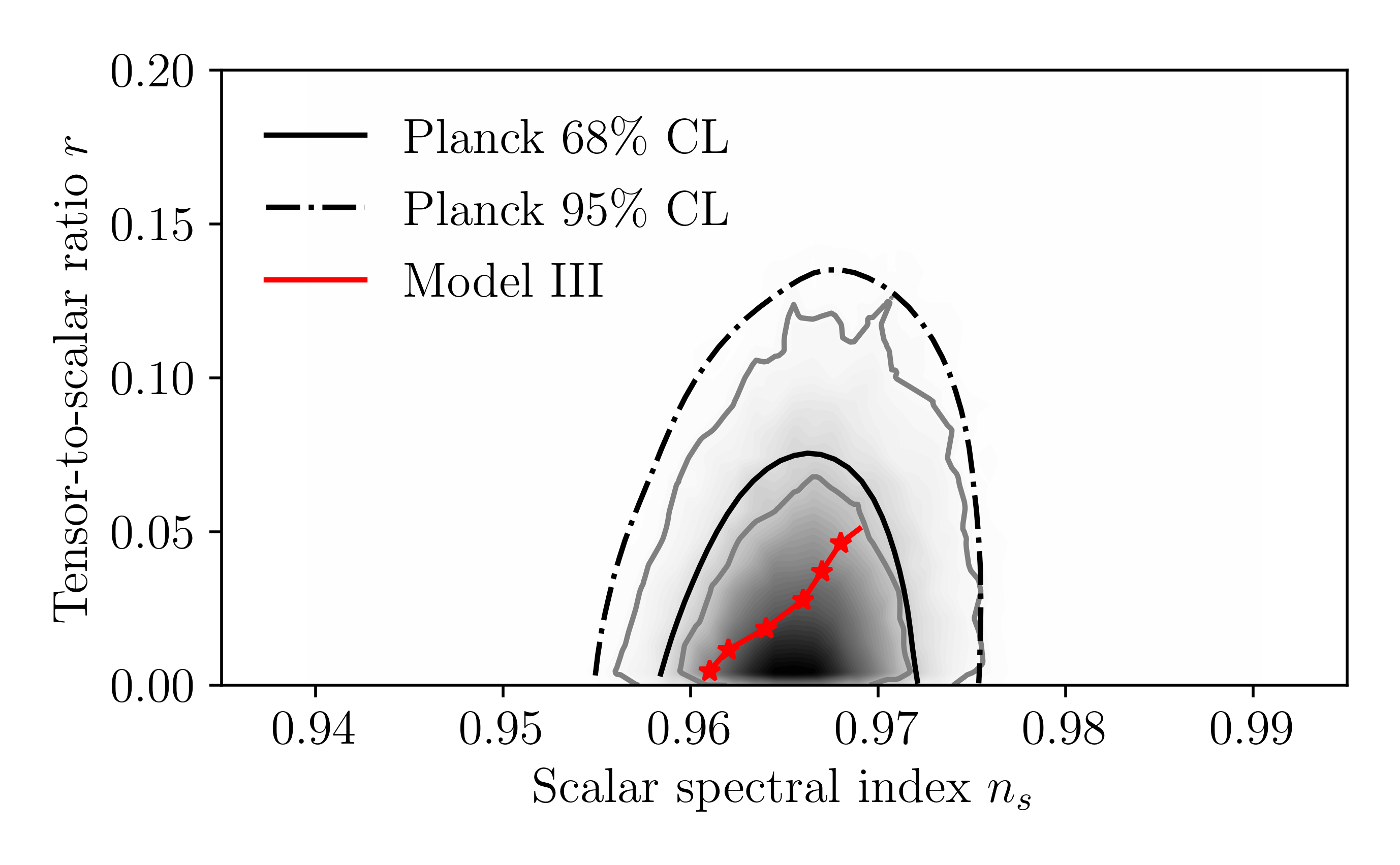
Figure 5: Planck 2018 Likelihood Curves for the Model III for $r=\delta/N^{3}$.

The potential of the scalar field is,

$$\centering V(N)=\frac{3}{4\kappa^{4}\left(C_{2}-2C_{1}\sqrt{\frac{6}{N^{3}}}N\left(e^{N}+N\operatorname{E}_{\frac{1}{2}}\left(-N\right)\right)\right)},\@add@centering$$ (49)

and the $\lambda(N)$ function is,

$$\centering\lambda(N)=\frac{e^{-N}\left(-2C_{1}e^{N}\delta+C_{2}\sqrt{\frac{\delta}{N^{3}}}N^{2}-2C_{1}\delta N\operatorname{E}_{\frac{1}{2}}\left(-N\right)\right)}{8C_{1}N^{2}}.\@add@centering$$ (50)

Once again for brevity we will present the full forms of the slow-roll indices and the analytic expression of the $n_{\mathcal{S}}$. The tensor spectral index of this model is,

$$\centering n_{T}=\frac{\delta\left(-\frac{2C_{2}\delta}{\sqrt{\frac{\delta}{N^{3}}}}+C_{1}e^{N}\left(-\delta+4\delta N+16N^{3}\right)+4C_{1}\delta N^{2}\operatorname{E}_{\frac{1}{2}}\left(-N\right)\right)}{16N^{4}\left(-2C_{1}e^{N}\delta+C_{2}\sqrt{\frac{\delta}{N^{3}}}N^{2}-2C_{1}\delta N\operatorname{E}_{\frac{1}{2}}\left(-N\right)\right)}.\@add@centering$$ (51)

The 2018 Planck Data constrain the scalar spectral index and thus the value of the parameter $\delta$. In this case $\delta<12096$. Varying the parameter $\delta$, and $n_{\mathcal{S}}$, we are able to calculate the exact value of the tensor-to-scalar ratio $r$ and the tensor spectral index $n_{T}$. Some of the different values we calculated to make the likelihood curve of this model are shown in Table 3.

Table 3: Different values for $\delta$ and $n_{\mathcal{S}}$ and the corresponding $n_{T}$ and $r$ for Model III.

$\delta$	r	$n_{\mathcal{S}}$	$n_{\mathcal{T}}$
1000	0.00463	0.961	0.92709
2500	0.011574	0.962	0.926818
6000	0.027778	0.966	0.927071
8000	0.037037	0.967	0.926526
11000	0.050926	0.969	0.92597

Using the data presented in the Table 3 we confront the model with the Planck 2018 data Planck:2018jri , and the results are presented in Fig. 5. As it can be seen in Fig. 5, also Model III is well fitted deeply in the Planck likelihood curves. Also in Fig. 6

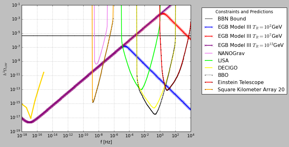
Figure 6: The $h^{2}$-scaled primordial gravitational waves energy spectrum for the Model III, versus the sensitivity curves of future primordial gravitational waves experiments.

we plot the $h^{2}$-scaled primordial gravitational waves energy spectrum for the Model III, and all the sensitivity curves of future primordial gravitational waves experiments for three reheating temperatures. As in all the previous cases, in this case too we chose the smallest value of the predicted tensor-to-scalar ratio and the corresponding blue-tilted spectral index. Thus Model III is also detectable by future gravitational waves experiments.

IV.4 Model IV: The Case with $r=\delta/N^{4}$

Now we consider a tensor-to-scalar ratio of the form,

$$\centering r=\frac{\delta}{N^{4}},\@add@centering$$ (52)

for which, the scalar coupling function is,

$$\centering\xi(N)=C_{2}+C_{1}\frac{\sqrt{\delta}}{N}\left(-e^{N}+N\operatorname{Ei}(N)\right),\@add@centering$$ (53)

where $C_{2}$, $C_{1}$ are integration constants and $N$ is the of $e$-foldings number.

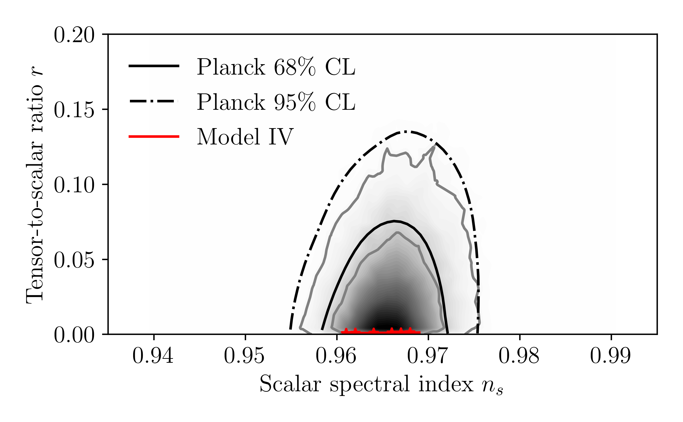
Figure 7: Planck 2018 Likelihood Curves for the Model IV for $r=\delta/N^{4}$.

The potential of the scalar field as a function of $N$ can be found by using Eq. (36) and it reads,

$$\centering V(N)=\frac{3}{4\kappa^{4}\left(C_{2}+C_{1}\sqrt{\frac{6}{N^{4}}}N\left(-e^{N}+N\operatorname{Ei}(N)\right)\right)}.\@add@centering$$ (54)

The function $\lambda$ for this model is,

$$\centering\lambda(N)=\frac{e^{-N}\left(C_{2}\frac{\sqrt{\delta}}{N^{2}}-\frac{C_{1}e^{N}\delta}{N^{3}}+\frac{C_{1}\delta\operatorname{Ei}\left(N\right)}{N^{2}}\right)}{8C_{1}}.\@add@centering$$ (55)

Repeating the work we have done in the previous cases we calculated the slow-roll indices using the above equations and then the scalar spectral index and the tensor spectral index (21),(22). For brevity we show only the tensor spectral index,

$$\centering n_{T}=\frac{\delta\left(-\frac{2C2\delta}{\sqrt{\frac{6}{N^{4}}}}+C1e^{N}\left(-\delta+2\delta N+16N^{4}\right)-2C_{1}\delta N^{2}\operatorname{Ei}(N)\right)}{16N^{5}\left(-C_{1}e^{N}\delta+C2\sqrt{\frac{6}{N^{4}}}N^{3}+C16N\operatorname{Ei}(N)\right)},\@add@centering$$ (56)

where $\delta<725760$ in order for the spectral index to satisfy the constraints imposed by the 2018 Planck Data. Some of the different values of the parameter $\delta$, $r$, the spectral index $n_{\mathcal{S}}$ and $n_{T}$ for this model are presented in Table 4.

Table 4: Different values for $\delta$ and $n_{\mathcal{S}}$ and the corresponding $n_{T}$ and $r$ for Model IV

$\delta$	$r$	$n_{\mathcal{S}}$	$n_{T}$
1000	0.000772	0.961	0.910203
500000	0.0385802	0,966	0.908538
100	$7.71605\cdot 10^{-6}$	0.966	0.912978
14000	0.00108	0.967	0.913392
16000	0.001223457	0.969	0.914448

Using the data presented in the Table 4 we confront the model with the Planck 2018 data Planck:2018jri in Fig. 7. As it can be seen in Fig. 7, Model IV is also well fitted deeply in the Planck likelihood curves. Also in Fig. 8

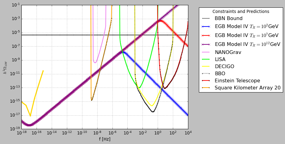
Figure 8: The $h^{2}$-scaled primordial gravitational waves energy spectrum for the Model IV, versus the sensitivity curves of future primordial gravitational waves experiments.

we plot the $h^{2}$-scaled primordial gravitational waves energy spectrum for the Model IV, versus the sensitivity curves of future primordial gravitational waves experiments, again for three reheating temperatures. As in all the previous models, we chose the smallest value of the predicted tensor-to-scalar ratio and the corresponding blue-tilted spectral index. This model too leads to a detectable energy power spectrum.

IV.5 Model V: The Case with $r=\delta/\sqrt{N}$

Let us now consider non-integer powers $d$ for the tensor-to-scalar ratio, and assume for simplicity that $d=\frac{1}{2}$ so the tensor-to-scalar ratio has the form,

$$\centering r=\frac{\delta}{\sqrt{N}}.\@add@centering$$ (57)

From Eq. (33) we find,

$$\centering\xi=C_{2}-C_{1}\sqrt{\delta}N^{\frac{3}{4}}\operatorname{E}_{\frac{1}{4}}(-N),\@add@centering$$ (58)

and the potential of the scalar field, according to Eq. (36), takes the form,

$$\centering V(N)=\frac{3}{4\kappa^{4}\left(C_{2}-C_{1}\sqrt{\delta}N^{\frac{3}{4}}\operatorname{E}_{\frac{1}{4}}(-N)\right)}.\@add@centering$$ (59)

The function $\lambda(N)$ in this case is,

$$\centering\lambda(N)=\frac{C_{2}\sqrt{\delta}}{8C_{1}}e^{-N}N^{-\frac{1}{4}}-\frac{\delta}{8}\sqrt{N}e^{-N}\operatorname{E}_{\frac{1}{4}}(-N).\@add@centering$$ (60)

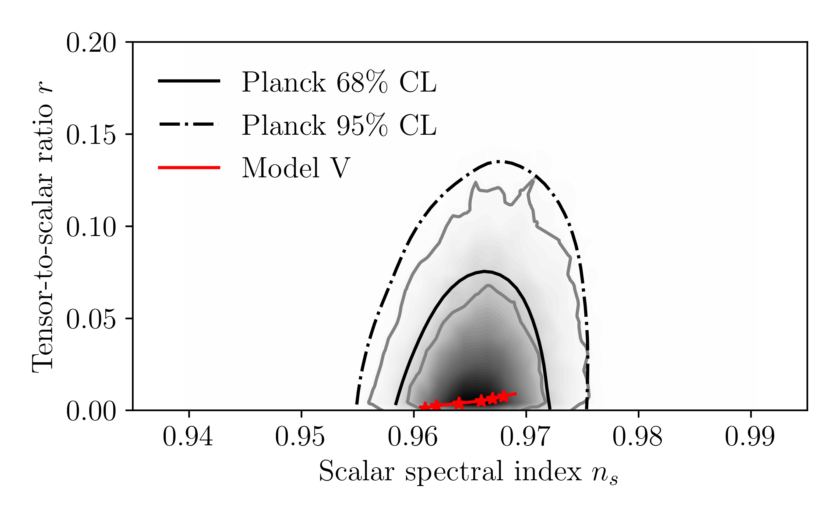
Figure 9: Planck 2018 Likelihood Curves for the Model V for$r=\delta/\sqrt{N}$.

Finally, the tensor spectral index is given by, (22),

$$\centering n_{T}=\frac{\delta\left(C_{1}e^{N}\left(\delta-16\sqrt{N}\right)+2C_{2}\right)}{16C_{1}\delta N^{\frac{3}{2}}\operatorname{E}_{\frac{1}{4}}(-N)-16C_{2}\sqrt{\delta}N^{\frac{3}{4}}}.\@add@centering$$ (61)

The upper limit of the $\delta$ parameter, in order for the tensor-to-scalar ratio $r$ to comply with $2018$ Planck constrains, is $0.433774$. By varying the parameter $\delta$ and the spectral index $n\mathcal{S}$ in Table 5 we present some values of the spectral index $n\mathcal{S}$ and $n_{T}$ for this model.

Table 5: Different values for $\delta$ and $n_{\mathcal{S}}$ and the corresponding $n_{T}$ and $r$ for Model V

$\delta$	$r$	$n_{\mathcal{S}}$	$n_{T}$
0.01	0.00129099	0.961	0.970617
0.02	0.00258199	0.962	0.970994
0.03	0.00387298	0.964	0.971902
0.04	0.00516398	0.966	0.972808
0.06	0.00774597	0.968	0.97356

Using the data presented in the Table 5 we confront the model with the Planck 2018 data Planck:2018jri in Fig. 9. As it can be seen in Fig. 9, Model V is well fitted deeply in the Planck likelihood curves. Also in Fig. 10

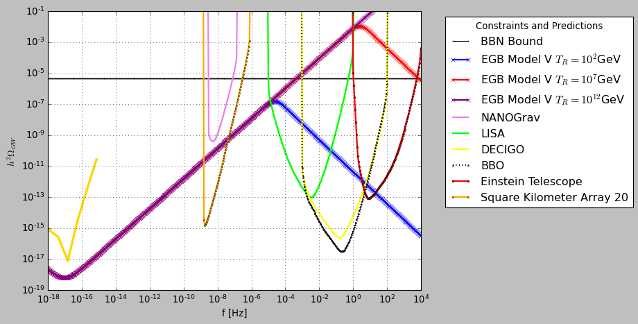
Figure 10: The $h^{2}$-scaled primordial gravitational waves energy spectrum for the Model V, versus the sensitivity curves of future primordial gravitational waves experiments.

we plot the $h^{2}$-scaled primordial gravitational waves energy spectrum for the Model V using the smallest value of the predicted tensor-to-scalar ratio and the corresponding blue-tilted spectral index. As it can be seen, this model too is promising observationally, since the predicted signal of inflationary stochastic gravitational waves is too large.

IV.6 Exponential Model VI: The case with $r=ae^{-bN}$

The last model we studied differs from the previous ones as the tensor-to-scalar ratio is not of the form of $r=\delta/N^{d}$ with $d>0$ but of the form of $r=ae^{-bN}$, where $a$, and $b$ are two free dimensionless parameters. Following the methodology of the previous sections, the scalar coupling function $\xi(N)$ is,

$$\centering\xi(N)=C_{2}-\frac{2C_{1}e^{N}\sqrt{ae^{-bN}}}{b-2}..\@add@centering$$ (62)

The potential of the scalar field as a function of the $e$-foldings number is,

$$\centering V(N)=\frac{3}{4\left(C_{2}-\frac{2C_{1}e^{N}\sqrt{ae^{-bN}}}{-2+b}\right)\kappa^{4}},\@add@centering$$ (63)

and the $\lambda(N)$ function which is essential for evaluating the slow-roll indices of the Einstein-Gauss-Bonnet theory is,

$$\centering\lambda(N)=\frac{1}{8}\left(-\frac{2ae^{-bN}}{-2+b}+\frac{C_{2}e^{-N}\sqrt{ae^{-bN}}}{C_{1}}\right).\@add@centering$$ (64)

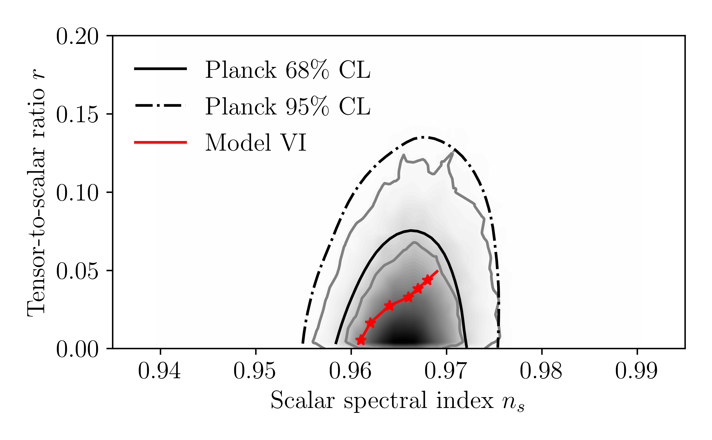
Figure 11: Planck 2018 Likelihood Curves for the Model VI for $r=ae^{-bN}$.

Using the above equations we compute the slow roll indices and the scalar and tensor spectral indices. The tensor spectral index for this model is,

$$n_{T}=\frac{a\left(a(-6+b)C_{1}e^{N}-2(-2+b)e^{bN}\left(8C_{1}e^{N}-C_{2}\sqrt{ae^{-bN}}\right)\right)}{32aC_{1}e^{N+bN}-16(-2+b)C_{2}e^{2bN}\sqrt{ae^{-bN}}}$$ (65)

In our study the variation of the parameter $a$ affects the value of the scalar to tensor ratio while the variation of the parameter $b$ affects the value of the tensor spectral index. A set of values of the ($n_{\mathcal{S}}$,$r$,$n_{T}$) with different values of the parameters $a$, and $b$ are given in Table 6.

Table 6: Different values for $a$, $b$ and $n_{\mathcal{S}}$ and the corresponding $n_{T}$ and $r$ for Model VI.

$a$	$b$	$r$	$n_{\mathcal{S}}$	$n_{T}$
100000000	0.4	0.00377513	0.961	0.538172
100000	0.3	0.001523	0.961	0.658666
100000000	0.43	0.00062402	0.966	0.501779
100000	0.3	0.001523	0.966	0.603673
100000000	0.4	0.00377513	0.969	0.543781

Using the data presented in the Table 6 we confront the model with the Planck 2018 data Planck:2018jri , and the results in this case, are presented in Fig. 11. As it can be seen in Fig. 11, Model VI is also well fitted deeply in the Planck likelihood curves. Also in Fig. 12

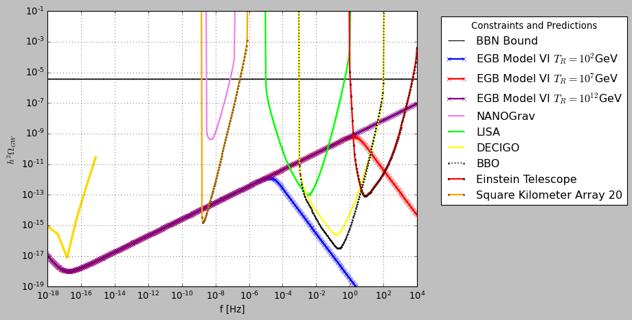
Figure 12: The $h^{2}$-scaled primordial gravitational waves energy spectrum for the Model VI, versus the sensitivity curves of future primordial gravitational waves experiments.

we plot the $h^{2}$-scaled primordial gravitational waves energy spectrum for the Model VI, versus the sensitivity curves of future primordial gravitational waves experiments for three reheating temperatures. In this case too, we chose the smallest value of the predicted tensor-to-scalar ratio and the corresponding blue-tilted spectral index. For this exponential model, and for large reheating temperatures, the predicted energy spectrum of the stochastic inflationary gravitational waves can be detected by most of the future experiments.

V Conclusions

In this paper we present a bottom-up reconstruction technique for obtaining viable inflation from GW170817-compatible Einstein-Gauss-Bonnet theories. Based on the formalism and approach of Ref. Oikonomou:2021kql , the bottom-up reconstruction technique is based on specifying the functional form of the tensor-to-scalar ratio as a function of the $e$-foldings number. From it we formally derived the scalar potential and the Gauss-Bonnet scalar coupling function, as functions of the $e$-foldings number. Accordingly, the calculation of the spectral indices of tensor and scalar perturbations is greatly simplified. We exemplified our new formalism by using several functional forms for the tensor-to-scalar ratio, chosen in such a way so that these are simple, and lead to an inflationary phenomenology compatible with the Planck 2018 data. We thoroughly studied several models of interest and we showed that the compatibility with the Planck 2018 data can be achieved for a general range of the free parameters. Furthermore, a notable feature of most of the models is that they lead to a blue-tilted tensor spectral index and as we showed, the energy spectrum of the inflationary primordial gravitational waves can be detectable by most of the future experiments on gravitational waves. Another notable feature is that for most of the models, the tensor-to-scalar ratio can take significantly smaller values than most of the $R^{2}$-like scalar field models.

A generalization of this work should include several higher powers of the Ricci scalar or non minimal coupling, since the presence of the Gauss-Bonnet term compels the Jordan frame picture. The theory would be more complicated, but it is compelling to make such generalizations due to the fact that if string corrections are present in the effective inflationary Lagrangian, then it is possible that higher powers of the Ricci scalar will be present, and specifically quadratic or cubic terms Codello:2015mba . With regard to non-minimal couplings, quantum corrections will be in the form of a conformal coupling Codello:2015mba . Thus generalizations of this work should include conformal couplings and possibly $R^{2}$ corrections separately, like in Refs. Odintsov:2020ilr and Odintsov:2020xji , respectively.

References

- (1) J. Baker, J. Bellovary, P. L. Bender, E. Berti, R. Caldwell, J. Camp, J. W. Conklin, N. Cornish, C. Cutler and R. DeRosa, et al. [arXiv:1907.06482 [astro-ph.IM]].
- (2) T. L. Smith and R. Caldwell, Phys. Rev. D 100 (2019) no.10, 104055 doi:10.1103/PhysRevD.100.104055 [arXiv:1908.00546 [astro-ph.CO]].
- (3) J. Crowder and N. J. Cornish, Phys. Rev. D 72 (2005), 083005 doi:10.1103/PhysRevD.72.083005 [arXiv:gr-qc/0506015 [gr-qc]].
- (4) T. L. Smith and R. Caldwell, Phys. Rev. D 95 (2017) no.4, 044036 doi:10.1103/PhysRevD.95.044036 [arXiv:1609.05901 [gr-qc]].
- (5) N. Seto, S. Kawamura and T. Nakamura, Phys. Rev. Lett. 87 (2001), 221103 doi:10.1103/PhysRevLett.87.221103 [arXiv:astro-ph/0108011 [astro-ph]].
- (6) S. Kawamura, M. Ando, N. Seto, S. Sato, M. Musha, I. Kawano, J. Yokoyama, T. Tanaka, K. Ioka and T. Akutsu, et al. [arXiv:2006.13545 [gr-qc]].
- (7) B. P. Abbott et al. [LIGO Scientific and Virgo], Phys. Rev. Lett. 119 (2017) no.16, 161101 doi:10.1103/PhysRevLett.119.161101 [arXiv:1710.05832 [gr-qc]].
- (8) B. P. Abbott et al. [LIGO Scientific, Virgo, Fermi-GBM and INTEGRAL], Astrophys. J. Lett. 848 (2017) no.2, L13 doi:10.3847/2041-8213/aa920c [arXiv:1710.05834 [astro-ph.HE]].
- (9) B. P. Abbott et al. “Multi-messenger Observations of a Binary Neutron Star Merger,” Astrophys. J. 848 (2017) no.2, L12 doi:10.3847/2041-8213/aa91c9 [arXiv:1710.05833 [astro-ph.HE]].
- (10) J. M. Ezquiaga and M. Zumalacárregui, Phys. Rev. Lett. 119 (2017) no.25, 251304 doi:10.1103/PhysRevLett.119.251304 [arXiv:1710.05901 [astro-ph.CO]].
- (11) T. Baker, E. Bellini, P. G. Ferreira, M. Lagos, J. Noller and I. Sawicki, Phys. Rev. Lett. 119 (2017) no.25, 251301 doi:10.1103/PhysRevLett.119.251301 [arXiv:1710.06394 [astro-ph.CO]].
- (12) P. Creminelli and F. Vernizzi, Phys. Rev. Lett. 119 (2017) no.25, 251302 doi:10.1103/PhysRevLett.119.251302 [arXiv:1710.05877 [astro-ph.CO]].
- (13) J. Sakstein and B. Jain, Phys. Rev. Lett. 119 (2017) no.25, 251303 doi:10.1103/PhysRevLett.119.251303 [arXiv:1710.05893 [astro-ph.CO]].
- (14) P. G. S. Fernandes, P. Carrilho, T. Clifton and D. J. Mulryne, Class. Quant. Grav. 39 (2022) no.6, 063001 doi:10.1088/1361-6382/ac500a [arXiv:2202.13908 [gr-qc]].
- (15) S. D. Odintsov, V. K. Oikonomou and F. P. Fronimos, Nucl. Phys. B 958 (2020), 115135 doi:10.1016/j.nuclphysb.2020.115135 [arXiv:2003.13724 [gr-qc]].
- (16) V. K. Oikonomou, Class. Quant. Grav. 38 (2021) no.19, 195025 doi:10.1088/1361-6382/ac2168 [arXiv:2108.10460 [gr-qc]].
- (17) J. c. Hwang and H. Noh, Phys. Rev. D 71 (2005) 063536 doi:10.1103/PhysRevD.71.063536 [gr-qc/0412126].
- (18) S. Nojiri, S. D. Odintsov and M. Sami, Phys. Rev. D 74 (2006) 046004 doi:10.1103/PhysRevD.74.046004 [hep-th/0605039].
- (19) G. Cognola, E. Elizalde, S. Nojiri, S. Odintsov and S. Zerbini, Phys. Rev. D 75 (2007) 086002 doi:10.1103/PhysRevD.75.086002 [hep-th/0611198].
- (20) S. Nojiri, S. D. Odintsov and M. Sasaki, Phys. Rev. D 71 (2005) 123509 doi:10.1103/PhysRevD.71.123509 [hep-th/0504052].
- (21) S. Nojiri and S. D. Odintsov, Phys. Lett. B 631 (2005) 1 doi:10.1016/j.physletb.2005.10.010 [hep-th/0508049].
- (22) M. Satoh, S. Kanno and J. Soda, Phys. Rev. D 77 (2008) 023526 doi:10.1103/PhysRevD.77.023526 [arXiv:0706.3585 [astro-ph]].
- (23) K. Bamba, A. N. Makarenko, A. N. Myagky and S. D. Odintsov, JCAP 1504 (2015) 001 doi:10.1088/1475-7516/2015/04/001 [arXiv:1411.3852 [hep-th]].
- (24) Z. Yi, Y. Gong and M. Sabir, Phys. Rev. D 98 (2018) no.8, 083521 doi:10.1103/PhysRevD.98.083521 [arXiv:1804.09116 [gr-qc]].
- (25) Z. K. Guo and D. J. Schwarz, Phys. Rev. D 80 (2009) 063523 doi:10.1103/PhysRevD.80.063523 [arXiv:0907.0427 [hep-th]].
- (26) Z. K. Guo and D. J. Schwarz, Phys. Rev. D 81 (2010) 123520 doi:10.1103/PhysRevD.81.123520 [arXiv:1001.1897 [hep-th]].
- (27) P. X. Jiang, J. W. Hu and Z. K. Guo, Phys. Rev. D 88 (2013) 123508 doi:10.1103/PhysRevD.88.123508 [arXiv:1310.5579 [hep-th]].
- (28) P. Kanti, R. Gannouji and N. Dadhich, Phys. Rev. D 92 (2015) no.4, 041302 doi:10.1103/PhysRevD.92.041302 [arXiv:1503.01579 [hep-th]].
- (29) C. van de Bruck, K. Dimopoulos, C. Longden and C. Owen, arXiv:1707.06839 [astro-ph.CO].
- (30) P. Kanti, J. Rizos and K. Tamvakis, Phys. Rev. D 59 (1999) 083512 doi:10.1103/PhysRevD.59.083512 [gr-qc/9806085].
- (31) A. E. Dominguez and E. Gallo, Phys. Rev. D 73 (2006), 064018 doi:10.1103/PhysRevD.73.064018 [arXiv:gr-qc/0512150 [gr-qc]].
- (32) H. Maeda, Class. Quant. Grav. 23 (2006), 2155 doi:10.1088/0264-9381/23/6/016 [arXiv:gr-qc/0504028 [gr-qc]].
- (33) S. G. Ghosh, Phys. Lett. B 704 (2011), 5-9 doi:10.1016/j.physletb.2011.08.066 [arXiv:1109.2371 [gr-qc]].
- (34) S. D. Maharaj, B. Chilambwe and S. Hansraj, Phys. Rev. D 91 (2015) no.8, 084049 doi:10.1103/PhysRevD.91.084049 [arXiv:1512.08972 [gr-qc]].
- (35) B. P. Brassel, S. D. Maharaj and R. Goswami, Phys. Rev. D 100 (2019) no.2, 024001 doi:10.1103/PhysRevD.100.024001
- (36) E. O. Pozdeeva, M. R. Gangopadhyay, M. Sami, A. V. Toporensky and S. Y. Vernov, Phys. Rev. D 102 (2020) no.4, 043525 doi:10.1103/PhysRevD.102.043525 [arXiv:2006.08027 [gr-qc]].
- (37) S. Vernov and E. Pozdeeva, Universe 7 (2021) no.5, 149 doi:10.3390/universe7050149 [arXiv:2104.11111 [gr-qc]].
- (38) E. O. Pozdeeva and S. Y. Vernov, Eur. Phys. J. C 81 (2021) no.7, 633 doi:10.1140/epjc/s10052-021-09435-8 [arXiv:2104.04995 [gr-qc]].
- (39) S. Koh, B. H. Lee, W. Lee and G. Tumurtushaa, Phys. Rev. D 90 (2014) no.6, 063527 doi:10.1103/PhysRevD.90.063527 [arXiv:1404.6096 [gr-qc]].
- (40) B. Bayarsaikhan, S. Koh, E. Tsedenbaljir and G. Tumurtushaa, JCAP 11 (2020), 057 doi:10.1088/1475-7516/2020/11/057 [arXiv:2005.11171 [gr-qc]].
- (41) G. Tumurtushaa, S. Koh and B. H. Lee, PoS ICHEP2018 (2019), 090 doi:10.22323/1.340.0090
- (42) I. Fomin, Eur. Phys. J. C 80 (2020) no.12, 1145 doi:10.1140/epjc/s10052-020-08718-w [arXiv:2004.08065 [gr-qc]].
- (43) M. De Laurentis, M. Paolella and S. Capozziello, Phys. Rev. D 91 (2015) no.8, 083531 doi:10.1103/PhysRevD.91.083531 [arXiv:1503.04659 [gr-qc]].
-
(44)
Scalar Field Cosmology, S. Chervon, I. Fomin, V. Yurov and
A. Yurov, World Scientific 2019,
doi:10.1142/11405 - (45) K. Nozari and N. Rashidi, Phys. Rev. D 95 (2017) no.12, 123518 doi:10.1103/PhysRevD.95.123518 [arXiv:1705.02617 [astro-ph.CO]].
- (46) S. D. Odintsov and V. K. Oikonomou, Phys. Rev. D 98 (2018) no.4, 044039 doi:10.1103/PhysRevD.98.044039 [arXiv:1808.05045 [gr-qc]].
- (47) S. Kawai, M. a. Sakagami and J. Soda, Phys. Lett. B 437, 284 (1998) doi:10.1016/S0370-2693(98)00925-3 [gr-qc/9802033].
- (48) Z. Yi and Y. Gong, Universe 5 (2019) no.9, 200 doi:10.3390/universe5090200 [arXiv:1811.01625 [gr-qc]].
- (49) C. van de Bruck, K. Dimopoulos and C. Longden, Phys. Rev. D 94 (2016) no.2, 023506 doi:10.1103/PhysRevD.94.023506 [arXiv:1605.06350 [astro-ph.CO]].
- (50) B. Kleihaus, J. Kunz and P. Kanti, Phys. Lett. B 804 (2020), 135401 doi:10.1016/j.physletb.2020.135401 [arXiv:1910.02121 [gr-qc]].
- (51) A. Bakopoulos, P. Kanti and N. Pappas, Phys. Rev. D 101 (2020) no.4, 044026 doi:10.1103/PhysRevD.101.044026 [arXiv:1910.14637 [hep-th]].
- (52) K. i. Maeda, N. Ohta and R. Wakebe, Eur. Phys. J. C 72 (2012) 1949 doi:10.1140/epjc/s10052-012-1949-6 [arXiv:1111.3251 [hep-th]].
- (53) A. Bakopoulos, P. Kanti and N. Pappas, Phys. Rev. D 101 (2020) no.8, 084059 doi:10.1103/PhysRevD.101.084059 [arXiv:2003.02473 [hep-th]].
- (54) W. Y. Ai, Commun. Theor. Phys. 72 (2020) no.9, 095402 doi:10.1088/1572-9494/aba242 [arXiv:2004.02858 [gr-qc]].
- (55) V. K. Oikonomou and F. P. Fronimos, [arXiv:2007.11915 [gr-qc]].
- (56) S. D. Odintsov, V. K. Oikonomou and F. P. Fronimos, Annals Phys. 420 (2020), 168250 doi:10.1016/j.aop.2020.168250 [arXiv:2007.02309 [gr-qc]].
- (57) V. K. Oikonomou and F. P. Fronimos, Class. Quant. Grav. 38 (2021) no.3, 035013 doi:10.1088/1361-6382/abce47 [arXiv:2006.05512 [gr-qc]].
- (58) S. D. Odintsov and V. K. Oikonomou, Phys. Lett. B 805 (2020), 135437 doi:10.1016/j.physletb.2020.135437 [arXiv:2004.00479 [gr-qc]].
- (59) S. D. Odintsov, V. K. Oikonomou, F. P. Fronimos and S. A. Venikoudis, Phys. Dark Univ. 30 (2020), 100718 doi:10.1016/j.dark.2020.100718 [arXiv:2009.06113 [gr-qc]].
- (60) S. A. Venikoudis and F. P. Fronimos, Eur. Phys. J. Plus 136 (2021) no.3, 308 doi:10.1140/epjp/s13360-021-01298-y [arXiv:2103.01875 [gr-qc]].
- (61) S. B. Kong, H. Abdusattar, Y. Yin and Y. P. Hu, [arXiv:2108.09411 [gr-qc]].
- (62) R. Easther and K. i. Maeda, Phys. Rev. D 54 (1996) 7252 doi:10.1103/PhysRevD.54.7252 [hep-th/9605173].
- (63) I. Antoniadis, J. Rizos and K. Tamvakis, Nucl. Phys. B 415 (1994) 497 doi:10.1016/0550-3213(94)90120-1 [hep-th/9305025].
- (64) I. Antoniadis, C. Bachas, J. R. Ellis and D. V. Nanopoulos, Phys. Lett. B 257 (1991), 278-284 doi:10.1016/0370-2693(91)91893-Z
- (65) P. Kanti, N. Mavromatos, J. Rizos, K. Tamvakis and E. Winstanley, Phys. Rev. D 54 (1996), 5049-5058 doi:10.1103/PhysRevD.54.5049 [arXiv:hep-th/9511071 [hep-th]].
- (66) P. Kanti, N. Mavromatos, J. Rizos, K. Tamvakis and E. Winstanley, Phys. Rev. D 57 (1998), 6255-6264 doi:10.1103/PhysRevD.57.6255 [arXiv:hep-th/9703192 [hep-th]].
- (67) D. Lovelock, J. Math. Phys. 12 (1971), 498-501 doi:10.1063/1.1665613
- (68) D. Lovelock, J. Math. Phys. 13 (1972), 874-876 doi:10.1063/1.1666069
- (69) Y. Akrami et al. [Planck], Astron. Astrophys. 641 (2020), A10 doi:10.1051/0004-6361/201833887 [arXiv:1807.06211 [astro-ph.CO]].
- (70) A. Codello and R. K. Jain, Class. Quant. Grav. 33 (2016) no.22, 225006 doi:10.1088/0264-9381/33/22/225006 [arXiv:1507.06308 [gr-qc]].
- (71) S. D. Odintsov, V. K. Oikonomou and F. P. Fronimos, Annals Phys. 424 (2021), 168359 doi:10.1016/j.aop.2020.168359 [arXiv:2011.08680 [gr-qc]].