Lense-Thirring effect on accretion flow from counter-rotating tori

Abstract

We study the accretion flow from a counter-rotating torus orbiting a central Kerr black hole (BH). We characterize the flow properties at the turning point of the accreting matter flow from the orbiting torus, defined by the condition $u^{\phi}=0$ on the flow torodial velocity. The counter-rotating accretion flow and jet-like flow turning point location along BH rotational axis is given. Some properties of the counter-rotating flow thickness and counter-rotating tori energetics are studied. The maximum amount of matter swallowed by the BH from the counter-rotating tori is determined by the background properties. The fast spinning BH energetics depends mostly on BH spin rather than on the properties of the counter-rotating fluids or the tori masses. The turning point is located in a narrow orbital corona (spherical shell), for photons and matter flow constituents, surrounding the BH stationary limit (outer ergosurface), depending on the BH spin–mass ratio and the fluid initial momentum only. The turning corona for jet-like-flow has larger thickness, it is separated from the torus flow turning corona and it is closer to the BH stationary limit. Turning points of matter accreting from torus and from jets are independent explicitly of the details of the accretion and tori model. The turning corona could be observable due to an increase of flow luminosity and temperature. The corona is larger on the BH equatorial plane, where it is the farthest from the central attractor, and narrower on the BH poles.

1 Introduction

Counter-rotating accreting tori orbiting a central attractor, particularly a Kerr black hole (BH), are a known possibility of the BH Astrophysics (Murray et al., 1999; Kuznetsov et al., 1999; Impellizzeri et al., 2019; Ensslin, 2003; Beckert&Falcke, 2002; Kim et al., 2016; Barrabes et al., 1995; Evans et al., 2010; Christodoulou et al., 2017; Nixon et al., 2011; Garofalo, 2013; Volonteri, 2010; Volonteri et al., 2003; Nixon et al., 2012a; Dyda et al., 2015; Amaro-Seoane et al., 2016; Zhang et al., 1997; Rao&Vadawale, 2012; Reis et al., 2013; Middleton et al., 2014; Morningstar et al., 2014; Cowperthwaite&Reynolds., 2012). In Active Galactic Nucleai (AGNs), corotating and counter-rotating tori, or strongly misaligned disks, as related to the central Kerr BH spin, can report traces of the AGNs evolution. Chaotical, discontinuous accretion can produce accretion disks with different rotation orientations with respect to the central Kerr BH where aggregates of corotating and counter-rotating toroids can be mixed (Dyda et al., 2015; Alig et al., 2013; Carmona-Loaiza et al., 2015; Lovelace&Chou, 1996; Lovelace et al., 2014; Pugliese&Stuchlík, 2015; Pugliese&Stuchlik, 2018a, b). Eventually, misaligned disks with respect to the central BH spin may characterize these strong attractors (Nixon et al., 2013; Doğan et al., 2015; Bonnerot et al., 2016; Aly et al., 2015).

Counter-rotating accretion disks can form in transient systems due to tidal disruption events and by episodic or prolonged phases of accretion, by galaxies merging, or binary (multiple) system components merging, or also from stellar formation in a counter-rotating cloud environment–see also Narayan et al. (2022); Tejeda et al. (2017); Wong et al. (2021); Porth et al. (2021); Zhang et al. (2015). Phenomena related to counter–rotation play very important role around BHs in the center of AGNs due to their possible complex accretion history; both co-rotating and counter-rotating accretion and equilibrium toroidal structures can orbit the central BH, being sometimes endowed with related jets (Pugliese&Stuchlik, 2021a, b, 2018c). Counter-rotating accretion structures are possible occasionally in the binary systems containing stellar mass BH, as in 3C120 (Kataoka et al., 2007; Cowperthwaite&Reynolds., 2012), the Galactic binary BHs (Zhang et al., 1997; Reis et al., 2013), BH binary system ((Morningstar et al., 2014) or (Christodoulou et al., 2017)). The counter-rotation phenomena and a wide range of their demonstration were discussed in a large variety of papers. Disk counter-rotation may also distinguish BHs with or without jets (Ensslin, 2003; Beckert&Falcke, 2002). Counter-rotating tori and jets were studied in relation to radio–loud AGN and double radio source associated with galactic nucleus (Evans et al., 2010; Garofalo et al., 2010). Observational evidence of counter-rotating disks has been provided by M87, observed by the Event Horizon TelescopeEvent Horizon Telescope Collaboration et al. (2019). In Middleton et al. (2014), counter-rotation of the extragalactic microquasars have been investigated as engines for jet emission powered by Blandford–Znajek processes.

BHs may accrete from disks having alternately corotating and counter-rotating senses of rotation (Murray et al., 1999). Less massive BH in counter-rotating configurations may "flip" to corotating configurations (this effect has been related to radio-loud systems turning into radio-quiet systems). Counter-rotating tori have been studied in more complex structures, for example featuring accreting disks/BH rotation "flip", i.e., alternate phases of cororation and counter-rotation accretion, or with the presence of relative counter-rotating layers in the same torus, vertically separated corotating-counter-rotating tori, or finally agglomerates of corotating and counter-rotating tori centered on one central Kerr BH orbiting on its equatorial plane (Pugliese&Stuchlík, 2015, 2016, 2017a). However, there is a crucial exception in the close vicinity of the BH horizon in the ergoregion where the accreting or non accreting, e.g. jets, matter must be co-rotating with the Kerr BH, from the point of view of distant observers, due to spacetime dragging (Pugliese&Stuchlik, 2021c). Therefore, it is of high relevance to study the turning of the accretion matter originally being in counter-rotation to the co–rotating motion, and its astrophysical consequences. In the present paper we study the turning effect in connection to matter accreting from counter-rotating toroidal structures, or the jets.

The toroidal structures are considered in the framework of the Ringed Accretion Disks model (RAD) developed in Pugliese&Montani (2015); Pugliese&Stuchlík (2015, 2016, 2017a) and widely discussed in subsequent papers(Pugliese&Stuchlik, 2017b, 2018b, 2018a, 2018c; Pugliese&Montani, 2018; Pugliese&Stuchlik, 2021a, 2020a, 2020b). Evidences of the presence of a cluster composed by an inner corotating torus and outer counter-rotating torus has been provided by Atacama Large Millimeter/submillimeter Array (ALMA). In Impellizzeri et al. (2019) counter-rotation and high-velocity outflow in the NGC1068 galaxy molecular torus were studied. NGC 1068 center hosts a super–massive BH within a thick dust and gas doughnut-shaped cloud. ALMA showed evidence that the molecular torus consists of counter-rotating and misaligned disks on parsec scales which can explain the BH rapid growth. From the observation of gas motion around the BH inner orbits, the presence of two disks of gas rotating in opposite directions was pointed out. It has been assumed that the outer disk could have been formed in a recent times from molecular gas falling. The inner disks follows the rotation of the galaxy, whereas the outer disk rotates (in stable orbit) the opposite way. The interaction between counter-rotating disks may enhance the accretion rate with a rapid multiple-phases of accretion.

This orbiting structure could be interpreted as a special RAD, composed by an outer disk counter-rotating relative to inner disk. This double structure with counter-rotating outer disk has been studied in particular in Pugliese&Stuchlík (2017a); Pugliese&Stuchlik (2017b); Pugliese&Montani (2018). These couples are generally stabilized (for tori collision) for high spins of the BHs, where the distance between the two tori can be very large, the inner co-rotating disk can be in the ergoregion and the two tori can be both in accretion phase, or the outer or the inner torus of the couple be in the accretion with a quiescent pair component. (The case of an orbiting pair of tori with an outer counter-rotating torus, differs strongly from the couple of an inner counter-rotating torus, limiting strongly the possibility of simultaneous accreting phase, mostly inner accretion counter-rotating torus and outer quiescent corotating torus, being possible only for slowly spinning attractors (Pugliese&Stuchlik, 2017b; Pugliese&Stuchlík, 2017a).)

Definition of torus counter-rotation is grounded on the hypothesis that the torus shares its symmetry plane and equatorial plane with the central stationary attractor and, within proper assumptions on the flow direction, the torus corotation or counter-rotation is a well defined property. In a more general frame, including the misaligned (or tilted) tori, these configuration symmetries do not hold–(Pugliese&Stuchlik, 2021a, 2020a, 2020b). In this context we expect that, because of the background frame–dragging, combined eventually with magnetic field or viscosity, and depending on tori inclination angle, the orbiting tilted torus can split in an inner part, forming eventually an equatorial co-rotating torus and an outer torus, producing a multiple disks structure composed by two orbiting tori centered on the BH with different relative rotation orientation, affecting the BH spin and mass. This complex phenomenon depends on several tori characteristic as its geometrical thickness, symmetries, maximum density points. In this context, the Lense–Thirring effect can express, being combined with the vertical stresses in the tori and the polar gradient of pressure, in the Bardeen–Petterson effect on the originally misaligned torus, broken due to the frame dragging and other factors as the fluids viscosity, in an inner corotating torus and an outer torus which may also be counter-rotating, where the BH spin can change under the action of the tori torques (Bardeen&Petterson, 1975; Nealon et al., 2015; Martin et al., 2014; King&Nixon, 2018; Nixon et al., 2012b, a; Lodato&Pringle, 2006; Scheuerl&Feiler, 1996; King et al., 2005). The frame-dragging can affect the accretion process, in particular for counter-rotating tori acting on the matter and photons flow from the accreting tori. The flow, having an initial counter-rotating component, due to the Lense–Thirring effect tends to reverse the rotation direction (toroidal component of the velocity in the proper frame) along its trajectory from the counter–rotating orbiting torus towards the BH. The flow, assumed to be free-falling into the central attractor, inherits some properties of the accreting configurations. Its trajectory is characterized by the presence of flow turning point, defined by the condition $u^{\phi}=\Omega=0$ on the axial component of the flow velocity and relativistic angular velocity relate to the distant static observer.

From methodological view–point we consider one-particle-species counter-rotating, geometrically thick toroids centered on the equatorial plane of a Kerr BH, considering "disk–driven" free–falling accretion flow constituted by matter and photons. We use a full GRHD Polish doughnut (PD) model (Abramowicz&Fragile, 2013), considering also the case of "proto-jets (or jets) driven" flows. (For the toroids influenced by the dark energy, or relict cosmological constant see Stuchlík (2005); Stuchlík, Slaný,&Kovář (2009); Stuchlík et al. (2020); Stuchlík&Kološ (2016); Stuchlík, Kološ,&Tursunov (2021)) Proto-jets are open HD toroidal configurations, with matter funnels along the BH rotational axis, associated to PD models, and emerging under special conditions on the fluid forces balance. Toroidal surfaces are the closed, and closed cusped PD solutions, proto-jets are the open cusped solutions of the PD model.

In this work we focus on the conditions for the existence of the turning point and the flow properties at this point. We discuss properties of the flow at the turning points distinguishing photon from matter components in the flow, and proto-jets driven and tori driven accreting flows. The turning point could be remarkably active part of the accreting flux of matter and photons, and we consider here particularly the region of the BH poles the equatorial plane, eventually characterized by an increase of the flow luminosity and temperature. However, we expect that the observational properties in this region could depend strongly on the processes timescales (related to the time flow reaches the turning points).

The paper is organized as follows:

In Sec. (2) we define the problem setup. In Sec. (2.1) equations and constants of motion are introduced. Details on tori models are in Sec. (2.2). Characteristics of the fluids at the flow turning point are the focus of Sec. (3). In Sec. (3.1) there is the analysis of the flow turning point, where definition of the turning point radius and plane is provided in Sec. (3.1.1). The analysis of the extreme values of the turning point radius and plane is in Sec. (3.1.3). Fluid velocity at the turning point is studied in Sec. (3.2). In Sec. (4) we specialize the investigation to the equatorial plane case, distinguishing the cases of flow turning point located on the equatorial plane of the central attractor in Sec. (4.1), with the discussion of the conditions on the counter-rotating flows with Carter constant $\mathcal{Q}=0$ in Sec. (4.1.1). Then the case of flow off the equatorial plane and general considerations on initial configurations are explored in Sec. (4.2). Turning points of the counter-rotating proto-jet driven flows are studied in Sec. (5). Verticality of the counter-rotating flow turning point (location along the BH rotational axis) is discussed in Sec. (6). Flow thickness and counter-rotating tori energetics are investigated in Sec. (7). In Sec. (8) there are some considerations on the fluids at the turning point. Discussion and concluding remarks follow in Sec. (9).

2 Counter-rotating accreting tori orbiting Kerr black holes

2.1 Equations and constants of geodesic motion

We consider counter-rotating toroidal configurations orbiting a central Kerr BH having spin $a=J/M\in]0,M]$, total angular momentum $J$ and the gravitational mass parameter $M$. The non-rotating case $a=0$ is the Schwarzschild BH solution while the extreme Kerr BH has dimensionless spin $a/M=1$. The background metric, in the Boyer-Lindquist (BL) coordinates $\{t,r,\theta,\phi\}$, is:

$$ds^{2}=-\left(1-\frac{2Mr}{\Sigma}\right)dt^{2}+\frac{\Sigma}{\Delta}dr^{2}+\Sigma d\theta^{2}+\left[(r^{2}+a^{2})+\frac{2Mra^{2}}{\Sigma}\sin^{2}\theta\right]\sin^{2}\theta d\phi^{2}-\frac{4rMa}{\Sigma}\sin^{2}\theta dtd\phi,$$ (1)

where

$$\Delta\equiv a^{2}+r^{2}-2rM;\quad\Sigma\equiv a^{2}\cos^{2}\theta+r^{2}.$$ (2)

In the following, where more convenient, we use dimensionless units where $M=1$. The horizons $r_{-}<r_{+}$ and the outer and inner stationary limits $r_{\epsilon}^{\pm}$ (ergosurfaces) are respectively given by

$$r_{\pm}\equiv M\pm\sqrt{M^{2}-a^{2}};\quad r_{\epsilon}^{\pm}\equiv M\pm\sqrt{M^{2}-a^{2}\cos\theta^{2}};$$ (3)

where $r_{+}<r_{\epsilon}^{+}$ on $\theta\neq 0$ and $r_{\epsilon}^{+}=2M$ in the equatorial plane $\theta=\pi/2$. The equatorial plane is a metric symmetry plane and the equatorial (circular) trajectories are confined on the equatorial plane as a consequence of the metric tensor symmetry under reflection through the plane $\theta=\pi/2$.

The constants of geodesic motions are

$$\mathcal{E}=-(g_{t\phi}\dot{\phi}+g_{tt}\dot{t}),\quad\mathcal{L}=g_{\phi\phi}\dot{\phi}+g_{t\phi}\dot{t},\quad g_{ab}u^{a}u^{b}=-\mu^{2},$$ (4)

$$\mathcal{Q}=(\cos\theta)^{2}\left[a^{2}\left(\mu^{2}-\mathcal{E}^{2}\right)+\left(\frac{\mathcal{L}}{\sin\theta}\right)^{2}\right]+(g_{\theta\theta}\dot{\theta})^{2};$$ (5)

with $u^{a}\equiv\{\dot{t},\dot{r},\dot{\theta},\dot{\phi}\}$, where $\dot{q}$ indicates the derivative of any quantity $q$ with respect the proper time (for $\mu=1$) or a properly defined affine parameter for the light-like orbits (for $\mu=0$). In Eqs (4) quantities $\mathcal{E}$ and $\mathcal{L}$ are defined from the Kerr geometry rotational Killing field $\xi_{\phi}=\partial_{\phi}$, and the Killing field $\xi_{t}=\partial_{t}$ representing the stationarity of the background. The constant $\mathcal{L}$ in Eq. (4) may be interpreted as the axial component of the angular momentum of a test particle following timelike geodesics and $\mathcal{E}$ represents the total energy of the test particle coming from radial infinity, as measured by a static observer at infinity, while $\mathcal{Q}$ in Eq. (5) is known as Carter constant. If $a>0$, then particles counter-rotation (corotation) is defined by $\mathcal{L}a<0$ ($\mathcal{L}a>0$).

From the constants of motion $(\mathcal{E},\mathcal{L})$ we obtain the relations for the velocity components $(u^{t},u^{\phi})$:

$$\dot{t}=\frac{g_{\phi\phi}\mathcal{E}+g_{t\phi}\mathcal{L}}{g_{t\phi}^{2}-g_{\phi\phi}g_{tt}},\quad\dot{\phi}=-\frac{g_{t\phi}\mathcal{E}+g_{tt}\mathcal{L}}{g_{t\phi}^{2}-g_{\phi\phi}g_{tt}}.$$ (6)

The relativistic angular velocity and the specific angular momentum are respectively

$$\Omega\equiv\frac{u^{\phi}}{u^{t}}=-\frac{\mathcal{E}g_{\phi t}+g_{tt}\mathcal{L}}{\mathcal{E}g_{\phi\phi}+g_{\phi t}\mathcal{L}}=-\frac{g_{t\phi}+g_{tt}\ell}{g_{\phi\phi}+g_{t\phi}\ell},\quad\ell\equiv\frac{\mathcal{L}}{\mathcal{E}}=-\frac{u_{\phi}}{u_{t}}=-\frac{g_{\phi\phi}u^{\phi}+g_{\phi t}u^{t}}{g_{tt}u^{t}+g_{\phi t}u^{\phi}}=-\frac{g_{t\phi}+g_{\phi\phi}\Omega}{g_{tt}+g_{t\phi}\Omega}.$$

If $a>0$ the fluid counter-rotation (corotation) is defined by $\ell a<0$ ($\ell a>0$). (Static observers, with four-velocity $\dot{\theta}=\dot{r}=\dot{\phi}=0$ cannot exist inside the ergoregion, then trajectories $\dot{r}\geq 0$, including particles crossing the stationary limit and escaping outside in the region $r\geq r_{\epsilon}^{+}$ are possible.).

For convenience we summarize the Carter equations of motion as follows (seeCarter (1968)):

$$\dot{t}=\frac{1}{\Sigma}\left[\frac{P\left(a^{2}+r^{2}\right)}{\Delta}-{a\left[a\mathcal{E}(\sin\theta)^{2}-\mathcal{L}\right]}\right],\quad\dot{r}=\pm\frac{\sqrt{R}}{\Sigma};\quad\dot{\theta}=\pm\frac{\sqrt{T}}{\Sigma},\quad\dot{\phi}=\frac{1}{\Sigma}\left[\frac{aP}{\Delta}-\left[{a\mathcal{E}-\frac{\mathcal{L}}{(\sin\theta)^{2}}}\right]\right];$$ (7)

where

$$P\equiv\mathcal{E}\left(a^{2}+r^{2}\right)-a\mathcal{L},\quad R\equiv P^{2}-\Delta\left[(\mathcal{L}-a\mathcal{E})^{2}+\mu^{2}r^{2}+\mathcal{Q}\right],\quad T\equiv\mathcal{Q}-(\cos\theta)^{2}\left[a^{2}\left(\mu^{2}-\mathcal{E}^{2}\right)+\left(\frac{\mathcal{L}}{\sin\theta}\right)^{2}\right].$$

2.2 Details on tori models

We specialize our analysis to GRHD toroidal configurations centered on the Kerr BH equatorial plane, which is coincident with the tori equatorial symmetry plane. Tori are composed by a one particle-specie perfect fluid, with constant fluid specific angular momentum $\ell$ (Abramowicz&Fragile, 2013; Pugliese&Montani, 2015; Pugliese&Stuchlík, 2015; Pugliese&Montani, 2021), total energy density $\varrho$ and pressure $p$, as measured by an observer comoving with the fluid with velocity $u^{a}$–Figs (2). We assume $\partial_{t}\mathbf{q}=0$ and $\partial_{\varphi}\mathbf{q}=0$, with $\mathbf{q}$ being a generic spacetime tensor. The continuity equation is identically satisfied and the fluid dynamics is governed by the Euler equation only. Assuming a barotropic equation of state ($p=p(\varrho)$), and orbital motion with $u^{\theta}=0$ and $u^{r}=0$, and by setting $\ell=$constant as a torus parameter fixing the maximum density points in the disk, the pressure gradients are regulated by the gradients of an effective potential function for the fluid $V_{eff}(r;\ell,a)$, which is invariant under the mutual transformation of the parameters $(a,\ell)\rightarrow(-a,-\ell)$.

The fluid effective potential, emerging from the GRHD constrain equation for the pressure, reads Abramowicz&Fragile (2013); Pugliese&Stuchlík (2015)

$$V_{eff}^{2}=\left(\frac{\mathcal{E}}{\mu}\right)^{2}={\frac{g_{t\phi}^{2}-g_{\phi\phi}g_{tt}}{g_{\phi\phi}+2g_{t\phi}\ell+g_{tt}\ell^{2}}},$$ (8)

assuming at the initial data $\dot{r}=\dot{\theta}=0$ and using the definitions of constants of motions $(\mu,\mathcal{E},\mathcal{L})$ of Eqs (4) and $\ell$ in Eqs (2.1). The extremes of the pressure in Eq. (10) are therefore regulated by the angular momentum distributions $\ell(r,\theta;a):\partial_{r}V_{eff}=0$ which, on the equatorial plane $\theta=\pi/2$, is

$$\ell^{\mp}\equiv\frac{a^{3}\mp r^{3/2}\Delta-a(4-3r)r}{a^{2}-(r-2)^{2}r}$$ (9)

for corotating $(-)$ and counter-rotating $(+)$ fluids respectively. Fluid effective potential defines the function $K(r)=V_{eff}(\ell(r))$. Cusped tori have parameter $K=K_{\times}\equiv K(r_{\times})\in]K_{center},1[\subset]K_{mso},1[$, where $K_{center}\equiv K(r_{center})$. (More in general we adopt the notation $q_{\bullet}\equiv q(r_{\bullet})$ for any quantity $q$ evaluated on a radius $r_{\bullet}$.). Super-critical tori have parameter $K=K_{s}\in]K_{\times},1[$ and they are characterized by an accretion throat (opening of the cusp), considered in more details in Sec. (7).

Torus cusp $r_{\times}$ is the minimum point of pressure and density in the torus corresponding to the maximum point of the fluid effective potential. The torus center $r_{center}$ is the maximum point of pressure and density in the torus, corresponding to the minimum point of the fluid effective potential. For the cusped co-rotating and counter-rotating tori, there is:

$$r_{center}=r_{\Upsilon}^{+},\quad r_{\times}=r_{\Upsilon}^{-},\quad\mbox{with}\quad r_{\Upsilon}^{\pm}(a,\ell)\equiv\frac{\lambda_{d}\pm\lambda_{e}}{12},\quad\mbox{where}$$ (10)

$$\lambda_{a}\equiv(a-2\ell)(a-\ell);\quad\lambda_{b}\equiv\left(2a^{2}-3a\ell+\ell^{2}\right)^{2},$$

$$\lambda_{c_{1}}\equiv 27a^{2}\ell^{4}(a-\ell)^{2}-144a^{2}\lambda_{a}(a-\ell)^{2}+16\lambda_{a}^{3}-72\ell^{2}\lambda_{a}(a-\ell)^{2}+432(a-\ell)^{4},$$

$$\lambda_{c_{2}}\equiv\left[16\lambda_{a}^{3}-72\lambda_{a}(a-\ell)^{2}\left(2a^{2}+\ell^{2}\right)+27(a-\ell)^{2}\left[a^{2}\left(\ell^{4}+16\right)-32a\ell+16\ell^{2}\right]\right]{}^{2}-256\left(2a^{2}-3a\ell+\ell^{2}\right)^{6},$$

$$\lambda_{c}\equiv 6\sqrt[3]{\lambda_{c_{1}}+\sqrt{\lambda_{c_{2}}}},$$

$$\lambda_{d}\equiv\sqrt{\frac{288\sqrt[3]{2}\lambda_{b}}{\lambda_{c}}+2^{2/3}\lambda_{c}+9\ell^{4}-48\lambda_{a}}+3\ell^{2},$$

$$\lambda_{e}\equiv 6\sqrt{\frac{3\left[32(a-\ell)^{2}+\ell^{2}(\ell^{4}-8\lambda_{a})\right]}{2\left(\lambda_{d}-3\ell^{2}\right)}-\frac{8\lambda_{a}}{3}-\frac{8\sqrt[3]{2}\lambda_{b}}{\lambda_{c}}-\frac{\lambda_{c}}{18\sqrt[3]{2}}+\frac{\ell^{4}}{2}}.$$

The matter outflows as consequence of the violation of mechanical equilibrium in the balance of the gravitational and inertial forces and the pressure gradients in the tori regulated by the fluid effective potential (Paczynski-Wiita (P-W) hydro-gravitational instability mechanism (Paczyński, 1980)). At the cusp ($r\leq r_{\times}$) the fluid may be considered pressure-free.

Accretion disk physics is regulated by the Kerr background circular geodesic structure constituted by the marginally circular orbit for timelike particles $r_{\gamma}^{\pm}$, which is also the photon circular orbit, the marginally bounded orbit, $r_{mbo}^{\pm}$, and the marginally stable circular orbit, $r_{mso}^{\pm}$ for corotating and counter-rotating motion. We consider also the radius $r_{\mathcal{M}}^{\pm}:\partial_{r}^{2}\ell=0$, and the set of radii $r_{(mbo)}^{\pm}$ and $r_{(\gamma)}^{\pm}$ and $r_{(\mathcal{M})}^{\pm}$ defined from

$$r_{\mathrm{(mbo)}}^{\pm}:\;\ell^{\pm}(r_{\mathrm{mbo}}^{\pm})=\ell^{\pm}(r_{\mathrm{(mbo)}}^{\pm})\equiv\mathbf{\ell_{\mathrm{mbo}}^{\pm}},\quad r_{(\gamma)}^{\pm}:\ell^{\pm}(r_{\gamma}^{\pm})=\ell^{\pm}(r_{(\gamma)}^{\pm})\equiv\mathbf{\ell_{\gamma}^{\pm}},\quad r_{(\mathcal{M})}^{\pm}:\ell^{\pm}(r_{\mathcal{M}}^{\pm})\equiv\ell_{\mathcal{M}}^{\pm}=\ell^{\pm}(r_{\mathcal{M}}^{\pm}),$$

$$\mbox{where}\quad r_{\gamma}^{\pm}<r_{\mathrm{mbo}}^{\pm}<r_{\mathrm{mso}}^{\pm}<r_{\mathrm{(mbo)}}^{\pm}<r_{(\gamma)}^{\pm}$$ (11)

see Figs (1).

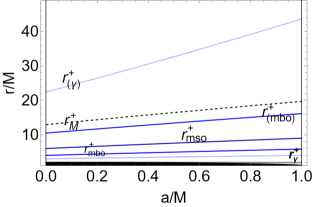
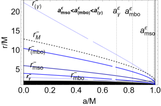
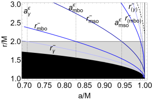
Figure 1: Kerr spacetime geodesic structure of Eqs (11) for corotating $(-)$ (center and right panels) and counter-rotating orbits $(+)$ (left panel) as functions of BH spin-mass ratio $a/M$, where black region is the BH at $r<r_{+}$, where $r_{+}$ is the outer BH horizon, gray region is the outer ergoregion $]r_{+},r_{\epsilon}^{+}[$ of the Kerr spacetime on the equatorial plane. Spins $\{a_{\gamma}^{\epsilon}\equiv 0.707107M,a_{mbo}^{\epsilon}\equiv 0.828427M,a_{mso}^{\epsilon}\equiv 0.942809M,a_{(mbo)}^{\epsilon}\equiv 0.989711M,a_{(\gamma)}^{\epsilon}\equiv 0.994298M\}$ are the geometries where the corotating geodesic structure radii coincide with the outer ergosurface $r_{\epsilon}^{+}=2M$ on the equatorial plane.

Ranges $(\mathbf{L_{1},L_{2},L_{3}})$ of fluids specific angular momentum $\ell$ govern the tori topology, according to the geodesic structure of Eqs (11), as follows:

$\mathbf{L_{1}}$:

for $\ell\in\mathbf{L_{1}}$ there are quiescent (i.e. not cusped) and cusped tori–where there is $\mp\mathbf{L_{1}}^{\pm}\equiv[\mp\ell_{mso}^{\pm},\mp\ell_{mbo}^{\pm}[$. The cusp is $r^{\pm}_{\times}\in]r^{\pm}_{mbo},r^{\pm}_{mso}]$ (with $K_{\times}^{\pm}<1$)) and the center with maximum pressure in $r^{\pm}_{center}\in]r^{\pm}_{mso},r^{\pm}_{(mbo)}]$.

$\mathbf{L_{2}}$:

for $\ell\in\mathbf{L_{2}}$ there are quiescent tori and proto-jets (open-configurations) –where there is $\mp\mathbf{L_{2}}^{\pm}\equiv[\mp\ell_{mbo}^{\pm},\mp\ell_{\gamma}^{\pm}[$. The cusp $r_{\times}^{\pm}\in]r_{\gamma}^{\pm},r_{mbo}^{\pm}]$ is associated to the proto-jets, with $K_{\times}>1$, and the center with maximum pressure is in $r_{center}^{\pm}\in]r_{(mbo)}^{\pm},r_{(\gamma)}^{\pm}]$;

$\mathbf{L_{3}}$:

for $\ell\in\mathbf{L_{3}}$ there are only quiescent tori where there is $\mp\mathbf{L_{3}}^{\pm}\equiv\mp\ell\geq\mp\ell_{\gamma}^{\pm}$ and the torus center is at $r^{\pm}_{center}>r_{(\gamma)}^{\pm}$,

–see Figs (2). Configurations with momentum in $\mathbf{L_{2}}$ range and $K>1$ are associated to (not-collimated) open structures, proto-jets, with matter funnels along the BH rotational axis–see Figs (2)–(Pugliese&Montani, 2015; Pugliese&Stuchlík, 2016; Pugliese&Stuchlik, 2018c, 2021b). Tori–driven and proto-jets-driven flows are flows originated from tori or proto-jet configurations respectively.

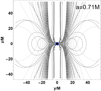
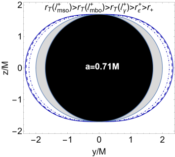
Figure 2: Counter-rotating flows. There is $r=\sqrt{y^{2}+z^{2}}$ and $\theta=\arccos({z}/r)$. Black central region is the central BH, gray region is the outer ergoregion. The BH spin-mass ratio is $a/M=0.71$. In this spacetime there are the limiting specific angular momenta $\{\ell_{mso}^{+}=-4.21319,\ell_{mbo}^{+}=-4.61534,\ell_{\gamma}^{+}=-6.50767\}$, defined in Eqs (11). Left panel shows the toroidal fluid equi-pressure (equi-density) surfaces evaluated at $\ell=-6.6$ (dotted-curves), $\ell=-5$ (dashed curves), $\ell=-4.5$ (gray curves). Closed toroids and the proto-jets (open funnels of matter parallel the BH rotational axis) are shown. Right panel is a zoom in the region close to the BH, $r_{+}$ is the BH horizon, and $r_{\epsilon}^{+}$ is the outer ergosurface radius. The counter-rotating flow turning points, $r_{{\mbox{\scriptsize{{T}}}}}$ of Eq. (15) are shown, evaluated for fluid specific angular momenta $\ell_{mso}^{+}$ (plain curve), $\ell_{mbo}^{+}$ (dashed curve) and $\ell_{\gamma}^{+}$ (dotted-dashed curve). The corona defined by the radii $(r_{\mbox{\scriptsize{{T}}}}(\ell_{mso}^{+})-r_{\mbox{\scriptsize{{T}}}}(\ell_{mbo}^{+}))$ ($(r_{\mbox{\scriptsize{{T}}}}(\ell_{\gamma}^{+})-,r_{\mbox{\scriptsize{{T}}}}(\ell_{mbo}^{+}))$) is the range of the counter-rotating flow turning points location from cusped tori (proto-jets) driven flows. Radii reach the maximum at the equatorial plane $(z=0)$–see Eqs (19), Eqs (44) and Figs (3).

In Figs (2) examples of different orbiting configurations and torus driven and proto-jets driven flow turning points are shown. Conditions for the turning points from proto-jets driven flows are discussed in more details in Sec. (5).

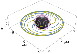
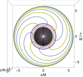
Figure 3: Tori driven counter-rotating flows turning points in the BH spacetime with spin-mass ratio $a/M=0.71$ and cusped tori with the fluid specific angular momentum $\ell=-4.5$, where is $\{z=r\cos\theta,y=r\sin\theta\sin\phi,x=r\sin\theta\cos\phi\}$ in dimensionless units. The limiting fluid specific angular momenta, defined in Eqs (11), are $\{\ell_{mso}^{+}=-4.21319,\ell_{mbo}^{+}=-4.61534,\ell_{\gamma}^{+}=-6.50767\}$–see also Figs (2). Left panel: the cusped torus orbiting the equatorial plane of the central BH. Central and right panels show a front and above view of the counter-rotating flow stream section on the equatorial plane from the torus inner edge (cusp) to the central BH. Black region is the central BH (region $r<r_{+}$, radius $r_{+}$ is the outer horizon). Flow turning point $r_{{\mbox{\scriptsize{{T}}}}}=2.31556M$ of Eqs (15),(19), (42) is plotted as the deep-purple curve. Radius $r_{{\mbox{\scriptsize{{T}}}}}$ lies in the turning corona defined by the range $(r_{\mbox{\scriptsize{{T}}}}(\ell_{mso}^{+})-r_{\mbox{\scriptsize{{T}}}}(\ell_{mbo}^{+}))$. Gray region is the outer ergosurface, light-purple shaded region is the region $r<r_{\mbox{\scriptsize{{T}}}}(\sigma_{\mbox{\scriptsize{{T}}}})$ (where $\sigma\equiv\sin^{2}\theta$)– see Figs (10). The analysis for photons is in Figs (3)

3 Fluids at the turning point of the azimuthal motion

3.1 Flow turning points

3.1.1 Definition of the turning point radius and plane

The flow turning point is defined by the condition $u^{\phi}=0$–see Figs (3). We thus obtain equation relating the motion constants of the infalling matter to the orbital turning point given generally by coordinates $(r_{\mbox{\scriptsize{{T}}}},\theta_{\mbox{\scriptsize{{T}}}})$. The value of the constant of motion $\ell=\mathcal{E}/\mathcal{L}$ is determined by the values of specific angular momentum $\ell$ at the cusp of the accreting torus that is assumed uniform accross the torus. In the following we use the notation $q_{\mbox{\scriptsize{{T}}}}$ or $q({\mbox{\scriptsize{{T}}}})$ for any quantity $q$ considered at the turning point, and $q_{0}=q(0)$ for any quantity $q$ evaluated at the initial point of the free-falling flow trajectory. In the special case where the initial flow particles location is coincident with the torus cusp, we use notation $q_{\times}$. In the following it will be useful to use the variable $\sigma\equiv\sin^{2}\theta$.

Conditions at the flow turning point can be found from the Carter equations of motion in Eqs (7), within the condition $u^{\phi}=0$ and using the constants of motion Eqs (4) and Eqs (5).

From the definition of constant $\ell$, fixed by the torus initial data, and turning point definition we obtain:

$$\ell=\left.-\frac{g_{t\phi}}{g_{tt}}\right|_{\mbox{\scriptsize{{T}}}}=\frac{2ar_{{\mbox{\scriptsize{{T}}}}}\sigma_{{\mbox{\scriptsize{{T}}}}}}{a^{2}(\sigma_{\mbox{\scriptsize{{T}}}}-1)-(r_{\mbox{\scriptsize{{T}}}}-2)r_{\mbox{\scriptsize{{T}}}}},$$ (12)

as on the turning point there is

$$\mathcal{E}=-g_{tt}({\mbox{\scriptsize{{T}}}})\dot{t}_{\mbox{\scriptsize{{T}}}},\quad\mathcal{L}=g_{t\phi}({\mbox{\scriptsize{{T}}}})\dot{t}_{\mbox{\scriptsize{{T}}}}.$$ (13)

Quantities $(\mathcal{E},\mathcal{L})$ are constants of motion, and could be found as $\mathcal{E}=\mathcal{E}_{\mbox{\scriptsize{{T}}}}$ and $\mathcal{L}=\mathcal{L}_{\mbox{\scriptsize{{T}}}}$ at the initial point where (for timelike particles on the equatorial plane) it could be assumed $V_{eff}(r_{\times})=\mathcal{E}$ at the cusp of the accreting torus, corresponding to an unstable circular geodesic. The parameters $(\mathcal{E},\mathcal{L})$ are thus the energy and axial angular momentum of the circular geodesic of the cusp in the equatorial plane of the Kerr geometry. We also note the independence of the turning point definition on the Carter constant $Q$, affecting the off-equatorial motion. We shall see that definition Eq. (12) defines, for fixed $\ell$, a spherical region surrounding the BH. For the turning point the crucial role is played by the constant specific angular momentum $\ell$ which is assumed uniform across the torus. To describe the more general situation then we mainly consider here $\ell$ fixed by the torus, and $(\mathcal{E},\mathcal{L})$ evaluated at the turning point as in Eqs. (13) within the (sign) constraint provided by the torus. (Note that there is $\mathcal{L}\ell<0$ with $\ell<0$ if $g_{t\phi}({\mbox{\scriptsize{{T}}}})<0$ where $\dot{t}_{\mbox{\scriptsize{{T}}}}>0$ which is the natural condition for the future-oriented particle motion (Balek et al., 1989), while there is $\mathcal{E}<0$ where $\dot{t}_{\mbox{\scriptsize{{T}}}}>0$ if $g_{tt}({\mbox{\scriptsize{{T}}}})>0$ in the ergoregion).

The flow turning point is located at a radius $r_{{\mbox{\scriptsize{{T}}}}}$ on a plane $\sigma_{\mbox{\scriptsize{{T}}}}$, related as follows:

$$\sigma_{{\mbox{\scriptsize{{T}}}}}(r_{{\mbox{\scriptsize{{T}}}}})=\frac{\ell\Delta_{{\mbox{\scriptsize{{T}}}}}}{a(a\ell-2r_{{\mbox{\scriptsize{{T}}}}})};$$ (14)

$$r_{{\mbox{\scriptsize{{T}}}}}(\sigma_{\mbox{\scriptsize{{T}}}})=\sqrt{a^{2}\left(\sigma_{\mbox{\scriptsize{{T}}}}+\frac{\sigma_{\mbox{\scriptsize{{T}}}}^{2}}{\ell^{2}}-1\right)-\frac{2a\sigma_{\mbox{\scriptsize{{T}}}}}{\ell}+1}-\frac{a\sigma_{\mbox{\scriptsize{{T}}}}}{\ell}+1.$$ (15)

Note that $\sigma_{\mbox{\scriptsize{{T}}}}(r_{\mbox{\scriptsize{{T}}}})$ and $r_{{\mbox{\scriptsize{{T}}}}}(\sigma_{{\mbox{\scriptsize{{T}}}}})$ depend on constant of motion $\ell$ only, holding for matter and photons, not depending explicitly from the normalization condition. Quantities $r_{{\mbox{\scriptsize{{T}}}}}$ and $\sigma_{{\mbox{\scriptsize{{T}}}}}$ are independent from the initial velocity $\dot{\sigma}_{{\mbox{\scriptsize{{T}}}}}$ or the constant $\mathcal{Q}$, therefore their dependence on the tori models and accretion process is limited to the dependence on the fluid specific angular momentum $\ell$ and the results considered here are adaptable to a variety of different general relativistic accretion models. .

By using Eq. (15) in Eqs (12), particles energy and angular momentum at the turning point are:

$$\mathcal{E}=\frac{a\sigma\dot{t}_{\mbox{\scriptsize{{T}}}}}{a\sigma_{\mbox{\scriptsize{{T}}}}-\ell},\quad\mathcal{L}=\frac{a\sigma\dot{t}_{\mbox{\scriptsize{{T}}}}\ell}{a\sigma_{\mbox{\scriptsize{{T}}}}-\ell},\quad\mbox{with}\quad\dot{t}_{\mbox{\scriptsize{{T}}}}=\mathcal{L}\left(\frac{1}{\ell}-\frac{1}{a\sigma_{\mbox{\scriptsize{{T}}}}}\right)$$ (16)

(and there is $\mathcal{E}\gtrless 0$ for $\ell\lessgtr a\sigma_{\mbox{\scriptsize{{T}}}}$, while there is $\mathcal{E}>0$ and $\ell>0$ for $\ell\in]0,a\sigma[$, assuming $\dot{t}_{\mbox{\scriptsize{{T}}}}>0$ which implies $\mathcal{L}\gtrless 0,\ell\lessgtr a\sigma_{\mbox{\scriptsize{{T}}}}$).

There is a turning point $(u^{\phi}=0)$ from Eq. (12), within the following conditions

$$a\in]0,1],\quad\ell<0\cup\ell>\ell_{lim}^{-}>0,\quad\mbox{where}\quad\ell_{lim}^{-}\equiv 2\left(\frac{1}{a}+\sqrt{\frac{1}{a^{2}}-1}\right)>\ell_{\gamma}^{-}>0,$$ (17)

respectively, where the following limits hold

$$\lim\limits_{\ell\rightarrow\pm\infty}r_{{\mbox{\scriptsize{{T}}}}}(\sigma_{\mbox{\scriptsize{{T}}}})=r_{\epsilon}^{+},\quad\lim\limits_{a\rightarrow 0}r_{{\mbox{\scriptsize{{T}}}}}(\sigma_{\mbox{\scriptsize{{T}}}})=r_{+}=2M,\quad\lim\limits_{\sigma\rightarrow 0}r_{{\mbox{\scriptsize{{T}}}}}(\sigma_{\mbox{\scriptsize{{T}}}})=r_{+},$$ (18)

see –Figs (9) and Figs (10). It should be stressed that there are no (time-like and photon-like) co-rotating turning points, solutions $u^{\phi}=0$ with the conditions $\ell>0$ with $\mathcal{E}>0$ and $\mathcal{L}>0$ ($u^{t}>0$), where $(\ell,\mathcal{E},\mathcal{L})$ are in Eqs (12). (Conditions (17) and limits (18) take into account only function $\ell_{\mbox{\scriptsize{{T}}}}$ in Eq. (12) providing a more general solution in $r>r_{+}$, dependent only on the condition $\ell=$constant, not necessarily related to the orbiting tori, and without considering the further constraints of $(\mathcal{E},\mathcal{L})=$constant). We will detail this aspect in Sec. (3.1.2).

From Eqs (18) we note that asymptotically, for $\ell$ very large in magnitude, function $r_{\mbox{\scriptsize{{T}}}}(\ell)$ approaches the ergosurface $r_{\epsilon}^{+}$ for any plane $\sigma_{\mbox{\scriptsize{{T}}}}$, from the region $r_{\mbox{\scriptsize{{T}}}}>r_{\epsilon}^{+}$ for counter-rotating flows, and $r_{\mbox{\scriptsize{{T}}}}<r_{\epsilon}^{+}$ for $\ell>0$—Figs (10). (Radius $r_{\mbox{\scriptsize{{T}}}}$ for $\ell>0$ must be in the ergoregion at any $\sigma$, while the counter-rotating fluids turning point must located out of the ergoregion.) At the BH poles, in the limit $\sigma\rightarrow 0$, the flow turning points coincide (according to the adopted coordinate frame) with the BH horizon. (This condition eventually holds also for the limit of static background where the eventual flow turning point is not induced by the frame-dragging.).

As pointed out in Sec. (2.2), a very large magnitude of $\ell$, explored in Eqs (18), corresponds to quiescent tori with $(\ell^{\pm})^{2}\gg(\ell^{\pm}_{\gamma})^{2}$, which can be very large and located far from the central BH (i.e. $r_{center}^{\pm}>r_{(\gamma)}^{\pm}$), for counter-rotating tori, and very close to the central attractor for co-rotating tori orbiting fast spinning BHs–Figs (1). As there is $\ell_{lim}^{-}>\ell_{\gamma}^{-}$, this condition holds for very large centrifugal component of the co-rotating quiescent torus force balance, for initial tori centered at $r>r_{(\gamma)}^{-}$, such radius is very far from the attractor for slower rotating BHs, and located in the ergoregion for fast spinning BH, i.e. for attractors with spins $a\geq a_{(\gamma)}^{\epsilon}\approx 0.994M$–Figs (1). The lower bound $\ell_{lim}^{-}$ in Eqs (17) for $\ell>0$, is independent from $\sigma$ and from the system initial data (initial fluid velocity and location) being a function of the BH spin $a/M$ only, and therefore it is independent from the tori models.

For the counter-rotating fluid turning points $\sigma_{\mbox{\scriptsize{{T}}}}(r_{{\mbox{\scriptsize{{T}}}}})$ there is

$$(\ell<0)\quad r_{{\mbox{\scriptsize{{T}}}}}\in]r_{\epsilon}^{+},r_{{\mbox{\scriptsize{{T}}}}}^{e}]\quad\mbox{with}\quad r_{{\mbox{\scriptsize{{T}}}}}^{e}\equiv\left.r_{\mbox{\scriptsize{{T}}}}\right|_{\sigma=1},$$ (19)

where $r_{{\mbox{\scriptsize{{T}}}}}^{e}$ is the turning point $r_{{\mbox{\scriptsize{{T}}}}}$ for $\sigma_{\mbox{\scriptsize{{T}}}}=1$– the turning point is located on the torus and the central attractor equatorial plane. (The role of equatorial plane in this problem is detailed in Sec. (4).). This implies that the turning point reaches its maximum value $r_{\mbox{\scriptsize{{T}}}}=2.45455M$ on the BH equatorial plane for the extreme Kerr BH spacetime. Remarkably, radius $r_{{\mbox{\scriptsize{{T}}}}}(\sigma_{\mbox{\scriptsize{{T}}}})$ in Eqs (15) and (14), depending on $\ell$ only, has no explicit dependence on the flow initial data. Therefore, at any plane $\sigma_{\mbox{\scriptsize{{T}}}}\in[0,1[$, the turning point radius $r_{\mbox{\scriptsize{{T}}}}$ is located in a range $r_{\mbox{\scriptsize{{T}}}}/M\in]2,2.45455[$, independently from other flow initial data.

More precisely, for a fixed value of $\ell$, function $r_{\mbox{\scriptsize{{T}}}}(\sigma)$, defines a surface, turning sphere, surrounding the central attractor. We can identify a turning corona, as the spherical shell defined by the limiting conditions on the radius $r_{\mbox{\scriptsize{{T}}}}(\sigma_{\mbox{\scriptsize{{T}}}})$ in the range $[r_{\mbox{\scriptsize{{T}}}}(\ell_{mbo}^{+})],r_{\mbox{\scriptsize{{T}}}}(\ell_{mso}^{+})]$, for tori driven counter-rotating flows, and $[r_{\mbox{\scriptsize{{T}}}}(\ell_{mbo}^{+})],r_{\mbox{\scriptsize{{T}}}}(\ell_{\gamma}^{+})]$ for proto-jets driven counter-rotating flows–see Figs (2,3,5,6,10). As shown in Figs (9), the circular region of turning points is delimited by the radii $r_{{\mbox{\scriptsize{{T}}}}}(\ell_{mso}^{\pm},\sigma_{\mbox{\scriptsize{{T}}}})>r_{{\mbox{\scriptsize{{T}}}}}(\ell_{mbo}^{\pm},\sigma_{\mbox{\scriptsize{{T}}}})$. The turning corona radii ($r_{\mbox{\scriptsize{{T}}}}(\ell_{\gamma}^{+}),r_{\mbox{\scriptsize{{T}}}}(\ell_{mbo}^{+}),r_{\mbox{\scriptsize{{T}}}}(\ell_{mso}^{+})$) vary little for the BH spin and plane $\sigma$. This also implies that the flow is located in restricted orbital range $(r_{{\mbox{\scriptsize{{T}}}}},\sigma_{{\mbox{\scriptsize{{T}}}}})$, localized in an orbital cocoon surrounding the central attractor outer ergosurface (reached at different times $t_{\mbox{\scriptsize{{T}}}}$ depending on the initial data–see Figs (9). Therefore the turning flow corona would be easily observable (depending on the values of $t_{\mbox{\scriptsize{{T}}}}$ range), characterized possibly by an increase of flow temperature and luminosity. As the flow characteristics at the turning point have a little dependence on the initial data, they hold to a remarkable extent also for different disks models. Radius $r_{\mbox{\scriptsize{{T}}}}(\sigma_{\mbox{\scriptsize{{T}}}})$ is in fact independent explicitly from the normalization conditions, as such the corona sets the location of the turning points for the photonic as well as particle components of the flow.

Although $r_{\mbox{\scriptsize{{T}}}}$ is bounded in a restricted orbital range, the turning point radius $r_{\mbox{\scriptsize{{T}}}}$ varies with $\sigma_{\mbox{\scriptsize{{T}}}}\in[0,1]$. The corona radii distance, $r_{\mbox{\scriptsize{{T}}}}(\ell_{mso}^{+})-r_{\mbox{\scriptsize{{T}}}}(\ell_{mbo}^{+})$, increases not monotonically with the BH spin-mass ratio and with the plane $\sigma$–Figs (5). (We also show in Fig. (4) some results concerning the case $\ell>0$.).

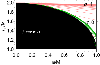
Figure 4: Considerations on the function $r_{\mbox{\scriptsize{{T}}}}$ for $\ell>0$. Black region is the BH at $r<r_{+}$ with dimensionless spin $a/M$, and $r_{+}$ is the outer BH horizon, the outer ergosurface is $r_{\epsilon}^{+}=2M$. Radii $r_{\mbox{\scriptsize{{T}}}}$ are shown on equatorial plane $\sigma=1$ (pink) and BH axis ($\sigma=0$) (green).

Decreasing $\sigma_{\mbox{\scriptsize{{T}}}}$, close to the BH poles, the $r_{\mbox{\scriptsize{{T}}}}$ range decreases, although the turning points location variation with $\sigma_{\mbox{\scriptsize{{T}}}}$ remains small–Figs (5). The vertical and maximum vertical location (along the BH rotational axis) of the turning point is studied in Sec. (6). Below we investigate more specifically the dependence of the turning point on the plane $\sigma$ and the BH spin-mass ratio $a/M$, proving the existence of a $r_{\mbox{\scriptsize{{T}}}}$ maximum for a variation of the BH spin $a/M$, distinguishing therefore counter-rotating accretions for different attractors.

In Figs (5) and Figs (6) we show the corona radii in dependence on the plane $\sigma_{\mbox{\scriptsize{{T}}}}$, particularly around the limiting plane value $\sigma=\sigma_{crit}=2\left(2-\sqrt{3}\right)$. For $\sigma<\sigma_{crit}$, there is $r_{\mbox{\scriptsize{{T}}}}<2M$ (related to the outer ergosurface location) and the radius $r_{\mbox{\scriptsize{{T}}}}$ decreases increasing the BH spin. Viceversa, at $\sigma\geq\sigma_{crit}$, turning radii are at $r_{\mbox{\scriptsize{{T}}}}>2M$, decreasing with the spin $a/M$. The turning corona could be therefore a very active part of the accreting flux of matter and photons, especially on the BH poles, and it is expected to be lightly more large (and rarefied at equal flow distribution along $\sigma\in[0,1]$ ) at the equatorial plane (however the time component $t_{\mbox{\scriptsize{{T}}}}$, and strongly different values of the turning point, could influence significantly details on the matter distribution relevant for the observation at the turning point). The maximum $r_{\mbox{\scriptsize{{T}}}}$ for the spin $a/M$ is in Figs (6).

In Figs (10) the case of slowly rotating BHs (small $a/M$) and fast rotating BHs are shown: for small $a/M$ the corona radii reduce to the orbits $r_{\mbox{\scriptsize{{T}}}}$, defining a spherical surface for turning points of particles and photons. The flow initial data however determine $\sigma_{\mbox{\scriptsize{{T}}}}$ and $r_{\mbox{\scriptsize{{T}}}}$ as independent variables, and the time component $t_{\mbox{\scriptsize{{T}}}}$ (related also to the accretion process time-scales and the details on inner disk active part where flow leaves the toroid). The analysis is repeated in Figs (12) for the proto-jets driven counter-rotating flows having specific momentum $\ell^{+}\in\mathbf{L^{+}_{2}}=]\ell_{\gamma}^{+},\ell_{mbo}^{+}]$.

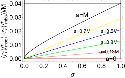
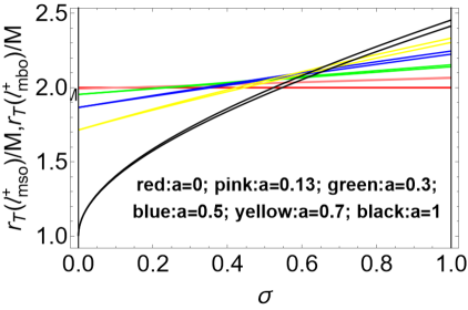
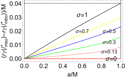
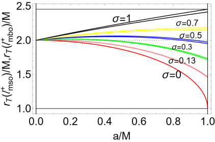
Figure 5: Turning radius $r_{{\mbox{\scriptsize{{T}}}}}$ of the tori driven counter-rotating flows, at the boundaries of the turning corona, is shown. The boundary radii are evaluated at the specific angular momenta $\ell=\ell_{mso}^{+}$ and $\ell=\ell_{mbo}^{+}$, defined in Eqs (11). Upper left panel: Corona radius, difference $(r_{{\mbox{\scriptsize{{T}}}}}(\ell_{mso}^{+})-r_{{\mbox{\scriptsize{{T}}}}}(\ell_{mbo}^{+})$, as function of the plane $\sigma\equiv\sin^{2}\theta$ is shown for different BH spin $a/M$ signed on the curves (upper left panel). and as function of $a/M$ for different plane $\sigma$ signed on the curve (bottom left panel). Radii $r_{{\mbox{\scriptsize{{T}}}}}(\ell_{mso}^{+})>r_{{\mbox{\scriptsize{{T}}}}}(\ell_{mbo}^{+})$ as functions of the plane $\sigma$, for different BH spins $a/M$ are shown in the upper right panel, and as functions of $a/M$, for different planes $\sigma$ in bottom right panel. In Figs (12) the analysis is repeated for the counter-rotating proto-jets driven flows.

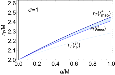
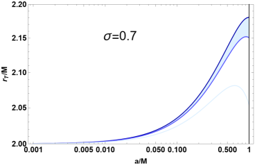
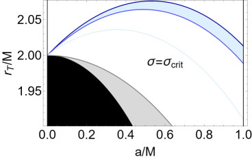
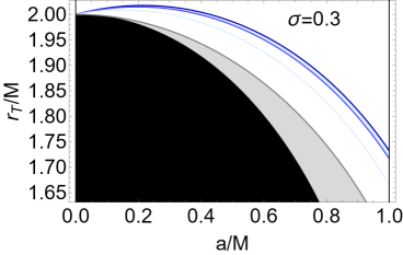
Figure 6: Extreme of the turning point radial coordinate, for fixed typical values of $\sigma$. Black region is the central BH (region $r<r_{+}$ where $r_{+}$ is the outer BH horizon), the outer ergosurface is $r_{\epsilon}^{+}=2M$. Gray region is the outer ergoregion, $]r_{+},r_{\epsilon}^{+}]$, for different planes $\sigma\equiv\sin^{2}\theta$ signed on the panels, where $\sigma=1$ is the equatorial plane and $\sigma_{crit}=2\left(2-\sqrt{3}\right)\approx 0.535898$. Counter-rotating flow turning points $r_{\mbox{\scriptsize{{T}}}}$ are shown as functions of BH spin-mass ratios $a/M$: there is $r_{{\mbox{\scriptsize{{T}}}}}(\ell_{mso}^{+})\geq r_{{\mbox{\scriptsize{{T}}}}}(\ell_{mbo}^{+})\geq r_{{\mbox{\scriptsize{{T}}}}}(\ell_{\gamma}^{+})$–see Eqs (11), plotted as dark-blue, blue and light-blue curves respectively. Note the different situations for planes smaller or larger than $\sigma_{crit}$, the curves maximum as functions of the dimensionless BH spin, and the spreading of the region $[r_{{\mbox{\scriptsize{{T}}}}}(\ell_{mbo}^{+}),r_{{\mbox{\scriptsize{{T}}}}}(\ell_{mso}^{+})]$ (light-blue shaded) defining the tori driven counter-rotating flow turning points corona are shown. The region $[r_{{\mbox{\scriptsize{{T}}}}}(\ell_{\gamma}^{+}),r_{{\mbox{\scriptsize{{T}}}}}(\ell_{mbo}^{+})]$ (white shaded) for the turning points of counter-rotating proto-jets driven flows is also shown.

In this analysis we addressed the conditions for the existence of a flow turning point and we explored the flow characteristics at the turning point. In Sec. (8), we also briefly investigate the flow at time $t>t_{\mbox{\scriptsize{{T}}}}$.

3.1.2 Further notes on flow rotation and double turning points

Flow rotation and constraints on the turning spheres

Turning point definition, as locus of points where $u^{\phi}=0$ in terms of $\ell$, defines a surface, turning sphere, surrounding the central BH, depending only on $\ell$ parameter. Here, we also study more in general function $\ell(u^{\phi}=0)$. However, further conditions have to be considered for the function $\ell_{\mbox{\scriptsize{{T}}}}$ when framed in the particles flow and tori flows turning points, namely: 1. constance of $(\mathcal{E}_{\mbox{\scriptsize{{T}}}},\mathcal{L}_{\mbox{\scriptsize{{T}}}})$ of Eqs (12), evaluated at the turning point with $\dot{t}$>0, implying $\ell=$constant. The constrained turning sphere is a general property of the orbits in the Kerr BH spacetime. It is clear that function $\ell_{\mbox{\scriptsize{{T}}}}=$constant is a more general solution, where conditions $\mathcal{E}=$constant and $\mathcal{L}=$constant depend on the specific trajectory. 2. Second constraint is the normalization condition at the turning point, $g_{\alpha\beta}u^{\alpha}u^{\beta}=\kappa$ (with $u^{\phi}=0$). 3. Third condition resolves into the description of the matter flows from the orbiting structures, translated into a constrain on the range of values for $\ell$, and defining the turning corona for proto-jets or accretion driven flows

The turning sphere and turning coronas are in fact a property of the background geometry, depending only on the spacetime spin. Therefore, in particular they describe also particles with $\dot{r}_{\mbox{\scriptsize{{T}}}}>0$ (outgoing particles) or particles moving along the central axis.

We shall study function $\ell_{\mbox{\scriptsize{{T}}}}$ in general, constraining it later in the different interpretative frameworks. An mentioned above, at the turning points the conditions $\ell>0$ (co-rotating case) with $(\mathcal{E}\gtrless 0,\mathcal{L}\gtrless 0)$ respectively, and $g_{\alpha\beta}u^{\alpha}u^{\beta}=\kappa$ with $\kappa=\{0,-1\}(u^{t}\gtrless 0)$ are never satisfied (while there is a spacelike solution ($\kappa=1$) in the ergoregion with $\mathcal{E}<0$ and $\mathcal{L}<0$ (and $u^{t}>0$)). A co-rotating $(\ell a>0)$ solution of function $\ell_{\mbox{\scriptsize{{T}}}}=$constant is also studied for completeness in this work.

For $u^{t}>0$, we can consider the following four cases (while notation T as been dropped for simplicity, it is intended all the quantities be evaluated at the turning point):

—

For $\ell<0$ with $(\mathcal{E}>0,\mathcal{L}<0)$, there are no turning points in the ergoregion.

Turning points are for

$$a\in]0,1]\quad(\mathcal{L}=\mathcal{L}_{bh},\mathcal{E}=\mathcal{E}_{bh}):\quad[(r\in]r_{+},2]\sigma\in]0,\sigma_{erg}[),(r>2,\sigma\in]0,1])],\quad\mbox{or}\quad(\sigma\in]0,1]r>r_{\epsilon}^{+}),$$

$$\mbox{where}\quad\mathcal{L}_{bh}\equiv-\frac{2ar\sigma u^{t}}{\Sigma},\quad\mathcal{E}_{bh}\equiv u^{t}\left[1-\frac{2r}{\Sigma}\right],\quad\sigma_{erg}\equiv\frac{(r-2)r}{a^{2}}+1,$$ (20)

(there is $\sigma_{erg}=\sigma:r_{\epsilon}^{+}(a;\sigma)=r$, for $r\in]r_{+},2]$ ). We consider now the second constraint, using the normalization condition at turning point.

For $\kappa=-1$ (flows particles) turning points are for:

$$a\in]0,1]\quad(\dot{r}^{2}=\dot{r}_{bh}^{2},\mathcal{L}=\mathcal{L}_{bh},\mathcal{E}=\mathcal{E}_{bh}),\quad\mbox{for}:$$

$$r\in]r_{+},2],\sigma\in]0,\sigma_{erg}[:(\dot{t}=\dot{t}_{bh},\dot{\theta}^{2}=0),(\dot{t}>\dot{t}_{bh},\dot{\theta}^{2}\in[0,\dot{\theta}_{bh}^{2}])];$$

$$r>2,\sigma\in]0,1]:(\dot{t}=\dot{t}_{bh},\dot{\theta}^{2}=0),(\dot{t}>\dot{t}_{bh},\dot{\theta}^{2}\in[0,\dot{\theta}_{bh}^{2}]),$$

or alternatively (21)

$$a\in]0,1],\sigma\in]0,1],r>r_{\epsilon}^{+},[(\dot{t}=\dot{t}_{bh},\dot{\theta}^{2}=0);(\dot{t}>\dot{t}_{bh},\dot{\theta}^{2}\in[0,\dot{\theta}_{bh}^{2}])],$$ (22)

where

$$\dot{t}_{bh}\equiv\sqrt{\frac{2r}{(r-2)r-a^{2}(\sigma-1)}+1},\quad\dot{\theta}_{bh}^{2}\equiv\frac{r\left[(r-2)\dot{t}^{2}-r\right]-a^{2}(\sigma-1)\left(\dot{t}^{2}-1\right)}{\Sigma^{2}},$$

$$\dot{r}_{bh}^{2}\equiv-\frac{\Delta\left[a^{4}(\sigma-1)^{2}\dot{\theta}^{2}+a^{2}(\sigma-1)\left[\dot{t}^{2}-1-2r^{2}\dot{\theta}^{2}\right]+r^{4}\dot{\theta}^{2}+r^{2}-(r-2)r\dot{t}^{2}\right]}{\Sigma^{2}}.$$ (23)

For null–like particles ($\kappa=0$) there is

$$a\in]0,1],\quad(\dot{r}^{2}=\dot{r}_{bh|0}^{2},\mathcal{L}=\mathcal{L}_{bh},\mathcal{E}=\mathcal{E}_{bh}),\quad\mbox{for}$$

$$(r\in]r_{+},2],\sigma\in]0,\sigma_{erg}[,\dot{\theta}^{2}\in[0,\dot{\theta}_{bh|0}^{2}]),(r>2,\sigma\in]0,1],\dot{\theta}^{2}\in[0,\dot{\theta}_{bh|0}^{2}]),\quad\mbox{ or alternatively}$$

$$\sigma\in]0,1],r>r_{\epsilon}^{+},\dot{\theta}^{2}\in[0,\dot{\theta}_{bh|0}^{2}],\quad\mbox{where}$$

$$\dot{\theta}_{bh|0}^{2}\equiv\frac{\dot{t}^{2}\left[(r-2)r-a^{2}(\sigma-1)\right]}{\Sigma^{2}};$$

$$\dot{r}_{bh|0}^{2}\equiv-\frac{\Delta\left[a^{4}(\sigma-1)^{2}\dot{\theta}^{2}+a^{2}(\sigma-1)\left(\dot{t}^{2}-2r^{2}\dot{\theta}^{2}\right)+r^{4}\dot{\theta}^{2}-(r-2)r\dot{t}^{2}\right]}{\Sigma^{2}}.$$ (24)

—

For completeness we also consider the case $\dot{t}>0$ and $(\mathcal{E}<0,\mathcal{L}>0)$ with $\ell<0$, where there is no turning point.

—

We consider now the case $\ell>0$ with $(\mathcal{E}>0,\mathcal{L}>0)$ (and $\dot{t}>0$). There are no turning points in this case.

—

The case $\ell>0$ with $(\mathcal{E}<0,\mathcal{L}<0)$ ($\dot{t}>0$) is relevant in the naked singularity (NS) spacetime, while in the BH geometries this condition does not correspond to any orbiting structure we consider in this work

There are solutions also for $\dot{t}<0$. In this case however energy $\mathcal{E}$ should be discussed accordingly, we consider this case for Kerr NSs in Pugliese&Stuchlík (2022). Finally we note that in this analysis we used three constants of motion,$(\mathcal{E},\mathcal{L})$ and the normalization condition, while Carter constant $\mathcal{Q}$ is independent on the sign of $(\mathcal{E},\mathcal{L})$ and therefore from the co-rotation or counter-rotation of the flow.

Double turning points

From Figs (10) we note the existence, for large $a$ and small $\sigma$, of two turning points at equal $\ell$ and fixed vertical axis $z_{\mbox{\scriptsize{{T}}}}=$constant. (There are always two turning points $z_{\mbox{\scriptsize{{T}}}}$ at fixed $y_{\mbox{\scriptsize{{T}}}}$ (on the vertical direction), while on the equatorial plane there is one turning point). Let us focus on the BH geometries turning points, from counter-rotating fluids, evaluated at the boundary values $\{\ell_{mso}^{+},\ell_{mbo}^{+},\ell_{\gamma}^{+}\}$. The presence of a maximum $z_{\mbox{\scriptsize{{T}}}}^{\max}$ of the turning point curve, solution of $\partial_{y_{\mbox{\scriptsize{{T}}}}}z_{\mbox{\scriptsize{{T}}}}^{+}=0$ is an indication of double turning points, where $r_{\mbox{\scriptsize{{T}}}}^{+}=\sqrt{(z_{\mbox{\scriptsize{{T}}}}^{+})^{2}+(y_{\mbox{\scriptsize{{T}}}}^{+})^{2}}$ and $\sigma_{\mbox{\scriptsize{{T}}}}=(y_{\mbox{\scriptsize{{T}}}}^{+})^{2}/((z_{\mbox{\scriptsize{{T}}}}^{+})^{2}+(y_{\mbox{\scriptsize{{T}}}}^{+})^{2})$. The existence of a solution $y_{\mbox{\scriptsize{{T}}}}^{+}=y_{\mbox{\scriptsize{{T}}}}(+)\neq 0:z_{\mbox{\scriptsize{{T}}}}^{+}=r_{+}$ indicates the presence of double turning point at $z_{\mbox{\scriptsize{{T}}}}^{+}\in[r_{+},z_{\mbox{\scriptsize{{T}}}}^{\max}[$ (and $y_{\mbox{\scriptsize{{T}}}}\leq y_{\mbox{\scriptsize{{T}}}}(+)$). Double turning points exist for large spins and small $\sigma$. In particular there is double turning point with $\ell_{mso}^{+}$ for $a>0.738315M$, with $\ell_{mbo}^{+}$ for $a>0.75M$ and with $\ell_{\gamma}^{+}$ for $a>0.785876M$ therefore, increasing the magnitude of the fluid specific angular momentum, double points are for larger BH spins. There is a maximum value of $y_{\mbox{\scriptsize{{T}}}}^{+}=y_{\mbox{\scriptsize{{T}}}}(+)>0$, increasing with the spin and, at fixed spin, decreasing with $\ell$ in magnitude. That is solution $z_{\mbox{\scriptsize{{T}}}}^{+}=r_{+}$ at $y_{\mbox{\scriptsize{{T}}}}(+)>0$ occurs for larger spin, increasing in magnitude the specific angular momentum $\ell^{+}$. The maximum distance from the axis of the turning point $y_{\mbox{\scriptsize{{T}}}}(+)>0:z_{\mbox{\scriptsize{{T}}}}^{+}=r_{+}$, increases with the BH spin in the sense of Figs (10) and decreases, increasing the angular momentum in magnitude. More specifically there is, at $a=M$, $y_{\mbox{\scriptsize{{T}}}}(+)=2.05274M$ ($\sigma_{\mbox{\scriptsize{{T}}}}=0.8082,r_{\mbox{\scriptsize{{T}}}}=2.28336M$) for $\ell_{mso}^{+}$, $y_{\mbox{\scriptsize{{T}}}}(+)=2.00812M$ ($\sigma_{\mbox{\scriptsize{{T}}}}=0.801293,r_{\mbox{\scriptsize{{T}}}}=2.24333M$) for $\ell_{mbo}^{+}$, $y_{\mbox{\scriptsize{{T}}}}(+)=1.8653M$ ($\sigma_{\mbox{\scriptsize{{T}}}}=0.776753,r_{\mbox{\scriptsize{{T}}}}=2.11645M$) for $\ell_{\gamma}^{+}$. (It is worth noting that, at $y_{\mbox{\scriptsize{{T}}}}=2M$ there is ($\sigma_{\mbox{\scriptsize{{T}}}}={4}/{5},r_{\mbox{\scriptsize{{T}}}}=\sqrt{5}M$).)

3.1.3 Analysis of the $(r_{\mbox{\scriptsize{{T}}}},\sigma_{\mbox{\scriptsize{{T}}}})$ extreme points

There are no extremes of the counter-rotating flow turning radius $r_{\mbox{\scriptsize{{T}}}}$ as function of $\sigma_{\mbox{\scriptsize{{T}}}}$, and there is $\partial_{\sigma_{\mbox{\scriptsize{{T}}}}}r_{{\mbox{\scriptsize{{T}}}}}>0$ as confirmed in Figs (5). It is worth noting that there is no extreme of $r_{{\mbox{\scriptsize{{T}}}}}$ as function of $\ell<0$. Considering relation (14), we see that are no solutions of $\partial_{r_{\mbox{\scriptsize{{T}}}}}\sigma_{\mbox{\scriptsize{{T}}}}=0$ with $\sigma_{\mbox{\scriptsize{{T}}}}\in[0,1]$, for $\ell<0$ and $r>r_{\epsilon}^{+}$. For counter-rotating flows there is a maximum of the turning point radius $r_{\mbox{\scriptsize{{T}}}}$ for the variation of the attractor dimensionless spin $a/M$. This implies that the frame-dragging acts differently for the BH spin mass-ratio, distinguishing different BH central attractors. The conditions can be expressed more precisely as follows:

There is $\partial_{a}r_{{\mbox{\scriptsize{{T}}}}}(\sigma_{\mbox{\scriptsize{{T}}}})=0$ for

$$a=a_{{max}}^{{\mbox{\scriptsize{{T}}}}}\equiv\frac{2\sigma\ell}{\sigma^{2}-\ell^{2}(1-\sigma)}\quad\mbox{with }\quad\sigma\in[0,\sigma^{a}_{max}],\quad\mbox{where}$$ (30)

$$\sigma^{a}_{max}\equiv\frac{1}{2}\left[\sqrt{\ell^{2}[(\ell-4)\ell+8]}-(\ell-2)\ell\right]\quad\mbox{and there is }\quad a_{max}^{{\mbox{\scriptsize{{T}}}}}(\sigma^{a}_{max})=M;$$

$$\mbox{equivalently for}\quad\sigma_{max}^{\mbox{\scriptsize{{T}}}}\equiv\frac{\sqrt{{\ell^{2}\left[a^{2}\left(\ell^{2}+4\right)+4(1-a\ell)\right]}}+\ell(2-a\ell)}{2a}$$ (31)

$$\mbox{or}\quad\ell_{max}^{\mbox{\scriptsize{{T}}}}\equiv-\frac{\sigma}{a(1-\sigma)}\left[1+\sqrt{{\left[1-a^{2}(\sigma-1)\right]}}\right]\quad\mbox{for}\quad\sigma\in]0,1[.$$

Note that incidentally these solutions coincide also with the maxima of $\sigma_{\mbox{\scriptsize{{T}}}}$ as function of $r_{\mbox{\scriptsize{{T}}}}$, that is there is:

$$\partial_{r_{\mbox{\scriptsize{{T}}}}}\sigma_{\mbox{\scriptsize{{T}}}}=0\quad\mbox{for}\quad r_{\mbox{\scriptsize{{T}}}}(\sigma_{max}^{\mbox{\scriptsize{{T}}}})=r_{max}^{\sigma}\equiv\frac{1}{2}\left[\sqrt{a\left[a\left(\ell^{2}+4\right)-4\ell\right]+4}+a\ell+2\right],\quad\mbox{with}\quad\sigma_{max}^{{\mbox{\scriptsize{{T}}}}}=\sigma_{\mbox{\scriptsize{{T}}}}(r_{max}^{\sigma})$$ (32)

—Figs (7). From the analysis of $r_{\mbox{\scriptsize{{T}}}}(\sigma_{\max}^{\mbox{\scriptsize{{T}}}})$, it is clear that a maximum exists for any spin $a/M$ (depending on $\ell$). The maximum increases with the BH spin, and the maximum extension of the corona radius is for the extreme Kerr BH with $a=M$, where $r_{{\mbox{\scriptsize{{T}}}}}/M\in[2.143,2.153]$, while the minimum is for the case of static attractor and coincides with the horizon $r=2M$. From the analysis of $\sigma_{\max}^{\mbox{\scriptsize{{T}}}}$, we find that the plane of the maximum point increases increasing the spin, reaching the maximum for $a=M$ where $\sigma_{\mbox{\scriptsize{{T}}}}\in]0.671,0.693[$. Similarly to $r_{\mbox{\scriptsize{{T}}}}$, plane $\sigma_{\mbox{\scriptsize{{T}}}}$ varies in a small range of values. From the analysis of the extremes according to the spin $a/M$, we find that the limiting value for the spin is the extreme Kerr BH, but for each spacetime the limiting plane is between the values for the limiting case for extreme Kerr BH and the static spacetime respectively, that is $\sigma\in[0.671,0.693]$ and $\sigma\in[0.629,0.649]$.

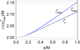
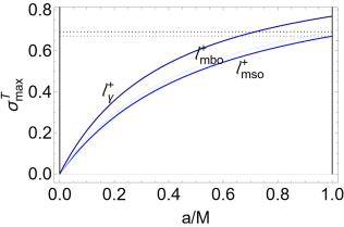
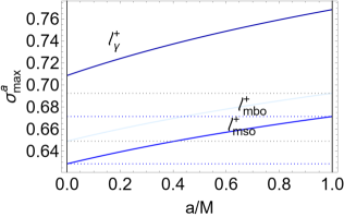
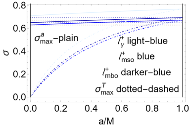
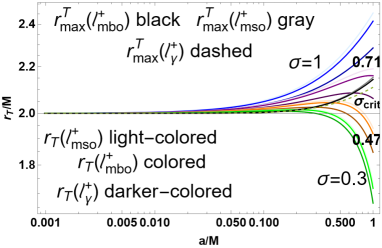
Figure 7: Counter-rotating flows. Upper line. Maximum extension of the turning radius $r_{{\mbox{\scriptsize{{T}}}}}$ (solutions of $\partial_{a}r_{{\mbox{\scriptsize{{T}}}}}(\sigma_{\mbox{\scriptsize{{T}}}})=0$ in Eq. (30)) as function of the BH spin-mass ratio $a/M$. There is $\sigma\equiv(\sin\theta)^{2}$. Blue (light-blue) curves are quantities evaluated on $\ell_{mso}^{+}$ ($\ell_{mbo}^{+}$), and darker-blue curves are quantities evaluated on $\ell_{\gamma}^{+}$. Limiting momenta $\ell_{mso}^{+}$, $\ell_{mbo}^{+}$, and $\ell_{\gamma}^{+}$ are defined in Eqs (11). Dotted lines are maximum and minimum values of $(r,\sigma)$, occurring for $a=0$ (the static spacetime limit) and $a=M$ (the extreme BH Kerr spacetime). Upper left panel: radius $r_{\mbox{\scriptsize{{T}}}}(\sigma_{max}^{\mbox{\scriptsize{{T}}}})=r_{max}^{\sigma}:\partial_{r_{\mbox{\scriptsize{{T}}}}}\sigma_{\mbox{\scriptsize{{T}}}}=0$ of Eq. (32) as function of $a/M$. Upper center panel: plane $\sigma_{max}^{{\mbox{\scriptsize{{T}}}}}=\sigma_{\mbox{\scriptsize{{T}}}}(r_{max}^{\sigma})$ of Eq. (31) as function of $a/M$. Upper right panel: Limiting plane $\sigma_{max}^{a}$, regulating the existence of the extreme spin $a_{{max}}^{{\mbox{\scriptsize{{T}}}}}$ of Eq. (30), is shown as function of $a/M$, where $a_{{max}}^{{\mbox{\scriptsize{{T}}}}}(\sigma_{max}^{a})=M$. Bottom left panel: limiting plane $\sigma_{max}^{a}$ and maximum plane $\sigma_{max}^{\mbox{\scriptsize{{T}}}}$ evaluated for $\ell_{mso}^{+}$, $\ell_{mbo}^{+}$ and $\ell_{\gamma}^{+}$, plotted as functions of $a/M$. Bottom right panel: Turning points $r_{\mbox{\scriptsize{{T}}}}$ on $\ell_{mso}^{+}$ (light-coloured curves) and $\ell_{mbo}^{+}$ (coloured curves) on different planes $\sigma$ signed on the curves ($\sigma=1$ is the equatorial plane). Black (gray) curve is the maximum $r_{max}^{{\mbox{\scriptsize{{T}}}}}$ on $\ell_{mbo}^{+}$ ($\ell_{mso}^{+}$). Analysis is also performed for limiting function $r_{\mbox{\scriptsize{{T}}}}(\ell_{\gamma}^{+})$ for counter-rotating proto-jet driven configurations as darker-colored curves.

3.2 Fluid velocities at the turning point

The time component of the flow velocity at the turning point is:

$$\dot{t}_{{\mbox{\scriptsize{{T}}}}}=\mathcal{L}\left(\frac{1}{\ell}-\frac{1}{a\sigma_{\mbox{\scriptsize{{T}}}}}\right)=\mathcal{E}\ell\left(\frac{1}{\ell}-\frac{1}{a\sigma_{\mbox{\scriptsize{{T}}}}}\right)$$ (33)

–(see Eq. (16)). Note that for counter-rotating flows ($\ell<0$) there is $\dot{t}_{{\mbox{\scriptsize{{T}}}}}>0$ at the turning point. (When $\ell>0$ and $\mathcal{L}>0$, there is $\dot{t}_{\mbox{\scriptsize{{T}}}}>0$ for $\ell<a\sigma_{{\mbox{\scriptsize{{T}}}}}$, which cannot occur in the tori model we consider here where there is $\ell>a>a\sigma_{{\mbox{\scriptsize{{T}}}}}$–see Sec. (3.1.2)).

Quantities $(\sigma_{\mbox{\scriptsize{{T}}}},r_{{\mbox{\scriptsize{{T}}}}},\dot{t}_{{\mbox{\scriptsize{{T}}}}})$ do not depend on the Carter constant $\mathcal{Q}$ (depending however on $\sigma$) and on the normalization condition, which represents a further constraint on the turning sphere, therefore they hold eventually for photons and matter. Notably $(\sigma_{\mbox{\scriptsize{{T}}}},r_{{\mbox{\scriptsize{{T}}}}},\dot{t}_{{\mbox{\scriptsize{{T}}}}})$ do not depend explicitly on the cusp initial location or the initial plane $\sigma_{0}$. This implies that, at the turning point, $r_{\mbox{\scriptsize{{T}}}}$ and $\dot{t}_{\mbox{\scriptsize{{T}}}}$ are explicitly regulated only by the torus momentum $\ell$, and $\mathcal{L}$ or $\mathcal{E}$ (in our case $K$ parameter) for $\dot{t}$. Therefore, the torus distance from the attractor or the precise identification of the torus "emission" region is not relevant for these features of the turning point. Nevertheless, quantities $(t_{{\mbox{\scriptsize{{T}}}}},\tau_{{\mbox{\scriptsize{{T}}}}})$ depend on the initial data, and ($\sigma_{\mbox{\scriptsize{{T}}}}$, $r_{{\mbox{\scriptsize{{T}}}}}$) can be obtained separately by solving the coupled equations for $\dot{\sigma}$ and $\dot{r}$, which depend on constant $\mathcal{Q}$, and therefore on $\sigma_{0}$ and $r_{0}$. These relations depend explicitly on the normalization conditions and the two constants of motion $\mathcal{L}$ and $\mathcal{E}=K$ (for timelike particles). However, if the torus is cusped then there is only one independent parameter, being $\ell$ sufficient to fix uniquely $\mathcal{E}=K(\ell)$.

In Fig. (8) we can see the evaluation of the $\left(T\right)\equiv\dot{t}_{\mbox{\scriptsize{{T}}}}\left(\tau_{\mbox{\scriptsize{{T}}}}\right)/\mathcal{E}$ at the turning point, on the turning corona extreme in Eq. (14). The analysis points out the small variation of these quantities according to the fluid momenta $\ell$, being $\left(T\right)\left(\ell_{{mso}}^{+}\right)<\left(T\right)\left(\ell_{{mbo}}^{+}\right)<\left(T\right)\left(\ell_{\gamma}^{+}\right)$.

Expressing $(\dot{r}_{{\mbox{\scriptsize{{T}}}}},\dot{\sigma}_{{\mbox{\scriptsize{{T}}}}})$ functions of $r_{{\mbox{\scriptsize{{T}}}}}$ we obtain

$$\dot{r}_{{\mbox{\scriptsize{{T}}}}}^{2}(r_{{\mbox{\scriptsize{{T}}}}})=\frac{(a\ell-2r_{{\mbox{\scriptsize{{T}}}}})\sqrt{\mathcal{E}^{2}\left[a(a-\ell)+r_{{\mbox{\scriptsize{{T}}}}}^{2}\right]^{2}-\Delta_{\mbox{\scriptsize{{T}}}}\left[\mathcal{E}^{2}(a-\ell)^{2}+\mu^{2}r_{{\mbox{\scriptsize{{T}}}}}^{2}+\mathcal{Q}\right]}}{2r_{{\mbox{\scriptsize{{T}}}}}\left[a(a-\ell)+r_{{\mbox{\scriptsize{{T}}}}}^{2}\right]},$$ (34)

$$\dot{\sigma}_{{\mbox{\scriptsize{{T}}}}}^{2}(r_{{\mbox{\scriptsize{{T}}}}})=-\frac{\ell(a\ell-2r_{{\mbox{\scriptsize{{T}}}}})^{2}\left[\Delta_{\mbox{\scriptsize{{T}}}}\left[\mathcal{Q}-\frac{ar_{{\mbox{\scriptsize{{T}}}}}(\mathcal{E}^{2}-\mu^{2})[2a+(r_{{\mbox{\scriptsize{{T}}}}}-2)\ell]}{a\ell-2r_{{\mbox{\scriptsize{{T}}}}}}\right]+[2a+(r_{{\mbox{\scriptsize{{T}}}}}-2)\ell]\mathcal{E}^{2}r_{{\mbox{\scriptsize{{T}}}}}\ell\right]}{16r_{{\mbox{\scriptsize{{T}}}}}^{3}\left[a(a-\ell)+r_{{\mbox{\scriptsize{{T}}}}}^{2}\right]^{2}[2a+(r_{{\mbox{\scriptsize{{T}}}}}-2)\ell]}.$$ (35)

Expressing $(\dot{r}_{{\mbox{\scriptsize{{T}}}}},\dot{\sigma}_{{\mbox{\scriptsize{{T}}}}})$ functions of $\sigma_{{\mbox{\scriptsize{{T}}}}}$ there is

$$\dot{\sigma}_{{\mbox{\scriptsize{{T}}}}}^{2}(\sigma_{{\mbox{\scriptsize{{T}}}}})=-\frac{\ell^{4}\left[\mathcal{E}^{2}(\sigma_{{\mbox{\scriptsize{{T}}}}}-1)\left(\ell^{2}-a^{2}\sigma_{{\mbox{\scriptsize{{T}}}}}\right)+\sigma_{{\mbox{\scriptsize{{T}}}}}\left[a^{2}\mu^{2}(\sigma_{{\mbox{\scriptsize{{T}}}}}-1)+\mathcal{Q}\right]\right]}{16(\sigma_{{\mbox{\scriptsize{{T}}}}}-1)(\ell-a\sigma_{{\mbox{\scriptsize{{T}}}}})^{2}\hat{m}^{2}};$$ (36)

$$\dot{r}_{{\mbox{\scriptsize{{T}}}}}^{2}(\sigma_{{\mbox{\scriptsize{{T}}}}})=-\frac{\sqrt{\ell^{2}\mathcal{E}^{2}\left[a\ell-\left(\frac{\hat{m}^{2}}{\ell^{2}}+a^{2}\right)\right]^{2}-{a\sigma_{{\mbox{\scriptsize{{T}}}}}\left(2\hat{m}+a\ell^{2}\right)\left[\frac{\mu^{2}\hat{m}^{2}}{\ell^{2}}+\mathcal{E}^{2}(a-\ell)^{2}+\mathcal{Q}\right]}}}{2(a\sigma_{{\mbox{\scriptsize{{T}}}}}-\ell)\hat{m}}.$$ (37)

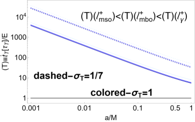
Figure 8: Quantity $\left(T\right)\equiv{\dot{t}_{\mbox{\scriptsize{{T}}}}\left(\tau_{\mbox{\scriptsize{{T}}}}\right)}/{\mathcal{E}}$ is plotted, at the counter-rotating flow turning points, at the extremes of the turning corona–Eq. (14)— for different planes $\sigma\equiv\sin^{2}\theta$, as functions of the BH spin $a/M$. Constant of motion $\mathcal{E}$ is defined in Eq. (4). The BH equatorial plane is at $\sigma=1$. Quantity $\left(T\right)$ is evaluated at the turning corona boundaries, for fluid specific angular momenta $\ell=\ell_{mso}^{+}$, $\ell=\ell_{mbo}^{+}$ and $\ell=\ell_{\gamma}^{+}$, defined in Eqs (11) for counter-rotating tori and proto-jets driven flows, there is $\left(T\right)\left(\ell_{{mso}}^{+}\right)<\left(T\right)\left(\ell_{{mbo}}^{+}\right)<\left(T\right)\left(\ell_{\gamma}^{+}\right)$.

Quantities $\dot{r}$ an $\dot{\theta}$ are in Eqs (7), the couple $(\dot{r},\dot{\theta})$ depends on $\mathcal{Q}$, whereas $\dot{r}$ depends explicitly on the normalization condition, distinguishing therefore explicitly photons from matter. On the equatorial plane there is $\mathcal{Q}=0$ only and only if $\dot{\theta}=0$ (more details on the equatorial plane case are discussed in Sec. (4)).

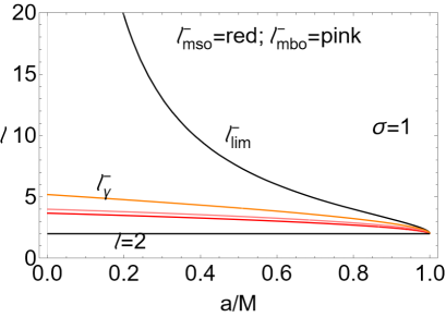
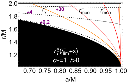
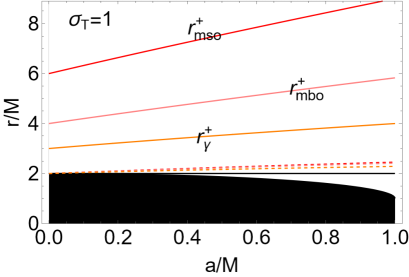
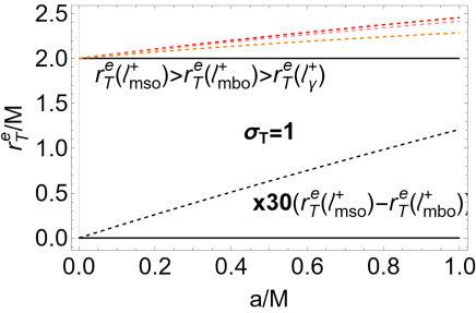
Figure 9: Allowed regions for the turning point of the azimuthal motion of the matter infalling from tori. Black region is the central BH at $r<r_{+}$, where $r_{+}$ is the outer BH horizon, the outer ergosurface is $r_{\epsilon}^{+}=2M$. The geodesic limiting values of the specific angular momentum $\ell^{\pm}=\{\ell_{mso}^{\pm},\ell_{mbo}^{\pm},\ell_{\gamma}^{\pm}\}$, plotted as functions of the BH dimensionless spin, are provided in Eqs (11). Panels show the function $r_{\mbox{\scriptsize{{T}}}}(\ell)$ on the equatorial plane $\sigma_{\mbox{\scriptsize{{T}}}}=1$ (where $\sigma\equiv\sin^{2}\theta$), for $\ell>0$ ($(-)$ upper line panels) and $\ell<0$ ($(+)$ bottom panels) fluids, analyzed in Sec. (4.) Upper panels show the situation for the $\ell>0$. Radius $r_{{\mbox{\scriptsize{{T}}}}}^{e}$ is in the ergoregion $]r_{+},r_{\epsilon}^{+}[$. Left upper panel: limiting tori specific angular momentum $\ell_{\lim}^{-}>\ell_{\gamma}^{-}$ of Eq. (17) as function of the BH spin–mass ratio $a/M$. The function limits the existence of a co-rotating fluid turning point at any plane $\sigma$. The limiting value $\ell=2$ is also shown. Upper right panel: corotating geodesic structure, defined in Eqs (11) (including the radii $r_{(mbo)}^{-},r_{(\gamma)}^{-}$, colored correspondingly to $r_{mbo}^{-},r_{\gamma}^{-}$), in the outer ergoregion, as functions of $a/M$. Dashed black line is the radius $r_{{\mbox{\scriptsize{{T}}}}}^{e}$ of Eq. (42) for specific angular momentum $\ell=(\ell_{\lim}^{-}+x)$ for different $x$ signed on the curves. Bottom left panel: counter-rotating geodesic structures of Eqs (11) and turning radii $r^{e}_{{\mbox{\scriptsize{{T}}}}}$ (dashed curves): there is $r^{e}_{\mbox{\scriptsize{{T}}}}(\ell_{mso}^{+})>r^{e}_{\mbox{\scriptsize{{T}}}}(\ell_{mbo}^{+})>r^{e}_{\mbox{\scriptsize{{T}}}}(\ell_{\gamma}^{+})$ as functions of $a/M$, black line is the outer ergosurface $r_{\epsilon}^{+}=2M$. Right panel shows a zoom on the radii $r^{e}_{\mbox{\scriptsize{{T}}}}(\ell_{mso}^{+})>r^{e}_{\mbox{\scriptsize{{T}}}}(\ell_{mbo}^{+})>r^{e}_{\mbox{\scriptsize{{T}}}}(\ell_{\gamma}^{+})$, dashed-black line is difference range $(r^{e}_{\mbox{\scriptsize{{T}}}}(\ell_{mso}^{+})-r^{e}_{\mbox{\scriptsize{{T}}}}(\ell_{mbo}^{+}))$, magnified for a factor of $(\mathbf{x30})$, providing the maximum range for the location of tori driven counter-rotating turning points on the equatorial plane–see Eqs (44) and (19).

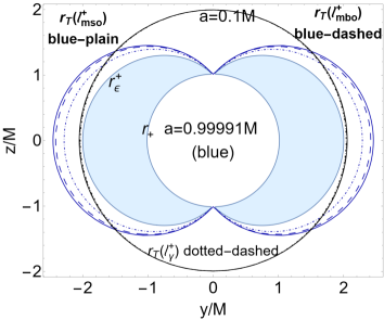
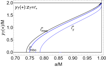
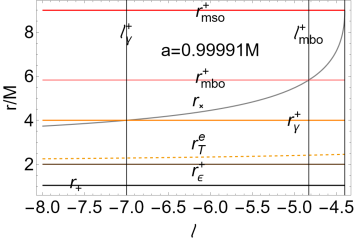
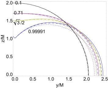
Figure 10: Turning points of the azimuthal motion of the counter-rotating flows in the $r-\theta$ plane for both tori and proto-jets. There is $r=\sqrt{y^{2}+z^{2}}$ and $\theta=\arccos({z}/r)$. Upper left panel: Counter-rotating flows turning point $r_{{\mbox{\scriptsize{{T}}}}}$ of Eq. (15) evaluated at fluid specific angular momenta $\ell_{mso}^{+}$ (plain) and $\ell_{mbo}^{+}$ (dashed), $\ell_{\gamma}^{+}$ (dotted-dashed) defined in Eqs (11), in the BH spacetime $a=0.1M$ (black curves) and $a=0.99991M$ (blue curves). The corona defined by the range $r_{\mbox{\scriptsize{{T}}}}(\ell_{mso}^{+})-r_{\mbox{\scriptsize{{T}}}}(\ell_{mbo}^{+})$ ($r_{\mbox{\scriptsize{{T}}}}(\ell_{\gamma}^{+})-r_{\mbox{\scriptsize{{T}}}}(\ell_{mbo}^{+})$) is orbital range of the turning points location for counter-rotating cusped tori (proto-jets) driven flows, which reaches its maximum on the equatorial plane $z=0$–see Eqs (44) and (19). Shaded blue region is the outer ergoregion $]r_{+},r_{\epsilon}^{+}]$, for the BH with spin $a=0.99991M$. Bottom right panel: solutions $y_{\mbox{\scriptsize{{T}}}}=y_{\mbox{\scriptsize{{T}}}}(+)\neq 0:z_{\mbox{\scriptsize{{T}}}}=r_{+}$ ($r_{+}$ is the BH outer horizon) indicating the presence of double turning point at $z_{\mbox{\scriptsize{{T}}}}>r_{+}$ (and $y_{\mbox{\scriptsize{{T}}}}\leq y_{\mbox{\scriptsize{{T}}}}(+)$). Center panels: counter-rotating flow turning point $r_{{\mbox{\scriptsize{{T}}}}}^{e}$ on the equatorial plane of Eq. (42) and counter-rotating tori cusp $r_{\times}\in]r_{mbo}^{+},r_{mso}^{+}]$ of Eq. (10) (for $\ell\in]\ell_{mbo}^{+},\ell_{mso}^{+}]$) as functions of the tori specific angular momentum $\ell$, for spacetime $a=0.99991M$ (left panel) and $a=0.1M$ (right panel). Radii of geodesic structures (horizontal lines), defined in Eqs (11), and related momenta $\ell$ (vertical lines), outer horizon $r_{+}$ and outer ergosurface on the equatorial plane $r_{\epsilon}^{+}=2M$ are also plotted. For proto-jets driven flows, there is $r_{\times}\in]r_{\gamma}^{+},r_{mbo}^{+}]$ cusp of a proto-jet for $\ell\in]\ell_{\gamma}^{+},\ell_{mbo}^{+}]$. Bottom panels show the analysis of the upper panel for the different BH spin–mass ratios $a/M$, signed on the curves. Colored regions are the BHs outer ergoregion $]r_{+},r_{\epsilon}^{+}[$ (the case $a=0.1M$ colored in black). Bottom left panel is a close-up view of the bottom right panel.

In Sec. (8) there is a discussion on the flow at the turning point.

4 The equatorial plane case

Motion on the equatorial plane of the Kerr central BH constitutes a relevant case for the problem of the flow turning point of infalling matter and photons.

We can distinguish the following two cases:

(I)

$\sigma_{0}=1$: the flow trajectory starts from the BH and torus equatorial plane. This situation can be framed in the standard accretion from a toroidal configuration centred on the BH and with symmetry and equatorial plane coincident with the BH equatorial plane. Accretion occurs at the torus inner edge $r_{\times}$ (for $\theta_{0}=\pi/2$). This case holds also for the proto-jets driven configurations where the cusp $r_{\times}$ is on the equatorial plane;

(II)

$\sigma_{{\mbox{\scriptsize{{T}}}}}=1$: in this case the flow turning point is on the equatorial plane.

Conditions (I) and (II) may hold in the same accretion model characterized by $\sigma_{0}=\sigma_{\mbox{\scriptsize{{T}}}}=1$, depending on the Carter constant $\mathcal{Q}$, holding for example in the special case where $\mathcal{Q}=0$ and $\dot{\theta}=\ddot{\theta}=0$.

In general, on the equatorial plane, $\theta=\pi/2$, from Eqs. (7) we find:

$$\dot{\theta}^{2}=\frac{\mathcal{Q}}{r^{4}},\quad\dot{t}=\frac{\mathcal{L}\left[a^{2}(r+2)-2a\ell+r^{3}\right]}{r\ell\Delta},\quad\dot{\phi}=\frac{\mathcal{L}[2a+(r-2)\ell]}{r\ell\Delta},$$ (38)

$$\dot{r}=\pm\frac{\sqrt{\frac{\mathcal{L}^{2}}{\ell^{2}}\left[a\ell-\left(a^{2}+r^{2}\right)\right]^{2}-\Delta\left[\frac{\mathcal{L}^{2}}{\ell^{2}}\left(\ell-{a}\right)^{2}+\mu^{2}r^{2}+\mathcal{Q}\right]}}{r^{2}}.$$

Furthermore, from the definition of $\mathcal{E}$, $\mathcal{L}$ and $\ell$, there is for $\theta=\pi/2$

$$\mathcal{E}=\frac{2a\dot{\phi}+(r-2)\dot{t}}{r},\quad\mathcal{L}=\frac{[a^{2}(r+2)+r^{3}]\dot{\phi}-2a\dot{t}}{r},\quad\ell=\frac{[a^{2}(r+2)+r^{3}]\Omega-2a}{2a\Omega+r-2},\quad\mathcal{Q}=r^{4}\dot{\theta}^{2}$$ (39)

$$\dot{t}=\frac{[a^{2}(r+2)+r^{3}]\mathcal{E}-2a\mathcal{L}}{r\Delta},\quad\dot{\phi}=\frac{2a\mathcal{E}+\mathcal{L}(r-2)}{r\Delta},\quad\Omega=\frac{2a+(r-2)\ell}{a^{2}(r+2)+r^{3}-2a\ell},$$ (40)

where $\Omega$ is the relativistic angular velocity.

4.1 Turning point on the equatorial plane: $\sigma_{{\mbox{\scriptsize{{T}}}}}=1$

From Eqs (39) on the turning point where $\dot{\phi}=\Omega=0$ we find:

$$\theta_{\mbox{\scriptsize{{T}}}}=\pi/2,\quad\dot{\phi}_{\mbox{\scriptsize{{T}}}}=\Omega_{\mbox{\scriptsize{{T}}}}=0,\quad\mathcal{E}=\frac{(r_{\mbox{\scriptsize{{T}}}}-2)\dot{t}_{\mbox{\scriptsize{{T}}}}}{r_{\mbox{\scriptsize{{T}}}}},\quad\mathcal{L}=-\frac{2a\dot{t}_{\mbox{\scriptsize{{T}}}}}{r_{\mbox{\scriptsize{{T}}}}},\quad\ell=\frac{2a}{2-r_{\mbox{\scriptsize{{T}}}}},\quad\dot{t}=\frac{a^{2}(r_{\mbox{\scriptsize{{T}}}}+2)+r_{\mbox{\scriptsize{{T}}}}^{3}}{r_{\mbox{\scriptsize{{T}}}}\Delta_{\mbox{\scriptsize{{T}}}}}\mathcal{E},$$ (41)

see also Eqs (16), Eqs (33), and Eqs (12),(14),(15). Assuming $\dot{t}_{\mbox{\scriptsize{{T}}}}>0$, there is $\mathcal{E}\lesseqgtr 0$ for $r_{\mbox{\scriptsize{{T}}}}\lesseqgtr 2M$ (located inside and out the ergoregion), occuring for $\ell\gtrless 0$ respectively. (The null limiting condition on $\mathcal{E}$ in the form (41) holds for $r_{\mbox{\scriptsize{{T}}}}=r_{\epsilon}^{+}=2M$ or for $\dot{t}_{\mbox{\scriptsize{{T}}}}=0$). From the equation for $\dot{t}_{\mbox{\scriptsize{{T}}}}$ we find $\dot{t}_{\mbox{\scriptsize{{T}}}}\mathcal{E}>0$, constraining the turning point location. (Relations in Eqs (41) are not independent, as on the equatorial plane $r_{{\mbox{\scriptsize{{T}}}}}^{e}\equiv 2\left(1-{a}/{\ell}\right)$). On the other hand, the energy $\mathcal{E}({\mbox{\scriptsize{{T}}}})$ does not depend explicitly on the BH spin $a$. Equally, there is $\mathcal{L}\lesseqgtr 0$ for $\dot{t}\gtreqless 0$ (where notably $\mathcal{L}=0$ for $\dot{t}_{\mbox{\scriptsize{{T}}}}=0$), while $\ell\lessgtr 0$ for $r_{\mbox{\scriptsize{{T}}}}\gtrless 2M$.

Therefore, for flow turning point on the attractor equatorial plane there is

$$\ell_{\mbox{\scriptsize{{T}}}}=\frac{2a}{r_{\mbox{\scriptsize{{T}}}}-2},\quad\mbox{for}\quad a\in]0,1],\quad\ell<0\cup\ell>\ell_{lim}^{-},$$ (42)

$$r_{{\mbox{\scriptsize{{T}}}}}=r_{{\mbox{\scriptsize{{T}}}}}^{e}\equiv 2\left(1-\frac{a}{\ell}\right),\quad\mbox{and}\quad\dot{t}_{{\mbox{\scriptsize{{T}}}}}=\dot{t}_{{\mbox{\scriptsize{{T}}}}}^{e}\equiv\mathcal{L}\left(\frac{1}{\ell}-\frac{1}{a}\right)=\mathcal{E}\ell\left(\frac{1}{\ell}-\frac{1}{a}\right)=-\frac{\mathcal{L}r_{{\mbox{\scriptsize{{T}}}}}}{2a}$$ (43)

–Figs (9) and Figs (10). As discussed in Sec. (3.1.1), the greater is the magnitude of $\ell$ (the far is the torus from the attractor) and the closer to $r_{\epsilon}^{+}$ the turning point is.

For counter-rotating flows, $r_{{\mbox{\scriptsize{{T}}}}}(\ell_{mso}^{+})$ is the outer turning corona radius, therefore for $\sigma_{\mbox{\scriptsize{{T}}}}=1$ there is $r_{{\mbox{\scriptsize{{T}}}}}^{e}\in[2M,r_{{\mbox{\scriptsize{{T}}}}}(\ell_{mso}^{+})[$ where $r_{{\mbox{\scriptsize{{T}}}}}(\ell_{mso}^{+})$ is maximum for the extreme BH. For $a=M$ the maximum extension (for the equatorial plane) is

$$r_{{\mbox{\scriptsize{{T}}}}}^{e}/M\in[2.41421,2.45455].$$ (44)

Notably there is $r_{{\mbox{\scriptsize{{T}}}}}^{e}/M<r_{\gamma}^{+}$–see Figs (9)

Furthermore, as clear from Eq. (43), for $\sigma=1$, the radius $r_{{\mbox{\scriptsize{{T}}}}}$ depends only on the ratio $\ell_{a}\equiv\ell/a$ (see also Pugliese&Montani (2015); Pugliese&Stuchlik (2021a)). There are no extreme of $r_{{\mbox{\scriptsize{{T}}}}}^{e}$, on the equatorial plane, with respect to $a/M$ and with respect to $\ell_{a}$.

From the definition of Carter constant $\mathcal{Q}$, there is from $\sigma_{\mbox{\scriptsize{{T}}}}=1$ (see Bicak&Stuchlik (1976))

$$\dot{\theta}_{\mbox{\scriptsize{{T}}}}^{2}=\frac{\mathcal{Q}}{r_{\mbox{\scriptsize{{T}}}}^{4}}=\frac{\mathcal{Q}\ell^{4}}{16\left(\ell-a\right)^{4}};\quad\mbox{and}\quad\dot{\theta}_{\mbox{\scriptsize{{T}}}}^{2}=0\quad\mbox{iff}\quad\mathcal{Q}=0.$$ (45)

This means that, within the condition $\theta_{\mbox{\scriptsize{{T}}}}=\pi/2$, the Carter constant $\mathcal{Q}$ can be different from zero and strictly positive $\mathcal{Q}>0$(necessary condition for so called orbital motion (Bicak&Stuchlik, 1976))– Eq. (45). On the other hand there is $\dot{\theta}_{\mbox{\scriptsize{{T}}}}^{2}=0$ iff $\mathcal{Q}=0$. Condition $\mathcal{Q}=0$ is related to condition $\theta_{0}=\pi/2$ on the initial toroidal configuration.

However the radial velocity component for the flow reads

$$\dot{r}_{\mbox{\scriptsize{{T}}}}=\pm\frac{\sqrt{\ell^{-2}\left[a\left(\ell^{2}+4\right)-4\ell\right]\left[\mathcal{L}^{2}(a-\ell)^{2}\left[a\left(\ell^{2}+4\right)-4\ell\right]-a\ell^{4}\left[(\mathcal{L}^{2}+4\mu^{2})\left(1-\frac{a}{\ell}\right)^{2}+\mathcal{Q}\right]\right]}}{4\left(\ell-a\right)^{2}},$$ (46)

$$\dot{r}_{\mbox{\scriptsize{{T}}}}=\pm\frac{\sqrt{\ell^{-2}\left[4\ell-a\left(\ell^{2}+4\right)\right]\left[\mathcal{L}^{2}(\ell[12a(a-\ell)+4\ell^{2}]-4a^{3})+a\mathcal{Q}\ell^{4}\right]}}{4(a-\ell)^{2}},$$

for particles and photons respectively. The radial velocity depends explicitly on $(\mathcal{L},\mathcal{Q},\mu,\ell)$ (sign $\pm$, for the ingoing flow $(-)$ or outgoing flow $(+)$, is not fixed).

From Eqs (46), for $\mathcal{Q}=0$ there is:

$$\dot{r}_{{\mbox{\scriptsize{{T}}}}}=\pm\frac{\sqrt{-\frac{(a-\ell)^{2}\left[a\left(\ell^{2}+4\right)-4\ell\right]\left[\mathcal{L}^{2}(\ell-a)+a\mu^{2}\ell^{2}\right]}{\ell^{2}}}}{2(a-\ell)^{2}},\quad\dot{r}_{{\mbox{\scriptsize{{T}}}}}=\pm\frac{\sqrt{\frac{\mathcal{L}^{2}(a-\ell)^{3}\left[a\left(\ell^{2}+4\right)-4\ell\right]}{\ell^{2}}}}{2(a-\ell)^{2}}.$$ (47)

for particles and photons respectively. Note that the radial velocity does not depend on the impact parameter only, but depends explicitly also on $\mathcal{L}$. The photonic $(\mu=0)$ relativistic velocity $\dot{r}_{\mbox{\scriptsize{{T}}}}/\dot{t}_{\mbox{\scriptsize{{T}}}}$ at the turning point, for $\mathcal{Q}=0$, depends on $\ell$ only (there is $\ell\mathcal{L}>0$), and this case is shown in Fig. (11) for $\ell$ in the range bounded by the liming momenta $\ell^{+}_{mso}>\ell_{mbo}^{+}>\ell_{\gamma}^{+}$ for counter-rotating tori and proto-jets driven photons –Figs (22).

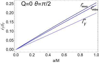
Figure 11: Relativistic photon radial velocity $\dot{r}_{\mbox{\scriptsize{{T}}}}/\dot{t}_{\mbox{\scriptsize{{T}}}}$ of Eq. (47) is plotted as functions of the BH spin $a/M$. The radial velocity is evaluated at the turning point for photons, on the equatorial plane, with Carter constant $\mathcal{Q}=0$ and for the specific angular momenta $\ell_{mso}^{+}$, $\ell_{mbo}^{+}$ and $\ell_{\gamma}^{+}$ defined in Eqs (11) for tori and proto-jets driven counter-rotating flows.

The photons relativistic radial velocity depends on the impact parameter $\ell$ inherited from the toroidal initial configurations, increasing in magnitude with the BH spin and decreasing with the increase of $\ell$ in magnitude, being therefore greater (in magnitude) for the tori-driven flows with respect to the proto-jets driven flows. On the other hand, the range of values for the relativistic radial velocity is larger for proto-jet driven flows, and increases with the BH spin $a/M$, distinguishing photons from proto-jets and tori driven flows, and narrowing the photon component radial velocities at the turning point in the tori driven counter-rotating flows.

4.1.1 Conditions on the counter-rotating flows with Carter constant $\mathcal{Q}=0$

From Eq. (5), it is clear that values of $\mathcal{Q}$ are limited by the constants of motion $(\mu,\mathcal{E},\mathcal{L})$, differing explicitly for photons and matter, when $\theta\neq\pi/2$ or $(\mathcal{E}^{2}-\mu^{2})\neq\left(\frac{\mathcal{L}}{a\sqrt{\sigma}}\right)^{2}$. The Carter constant is not restricted by the BH spin $a/M$ on the equatorial plane $\theta=\pi/2$, or for $\mu^{2}=\mathcal{E}^{2}$, or for $(\mathcal{E}^{2}-\mu^{2})=\left(\frac{\mathcal{L}}{a\sqrt{\sigma}}\right)^{2}$. (The second condition on the particle energy is related to the limiting conditions distinguishing proto–jets and tori driven flows. This condition and the third relation is briefly discussed below.)

According to Eq. (45) a zero Carter constant implies

$$\mathcal{Q}=0:\quad(\dot{\theta})^{2}=(\dot{\theta}_{\zeta})^{2}\equiv\frac{(\sigma-1)[a^{2}\sigma(\mu^{2}-\mathcal{E}^{2})+\mathcal{L}^{2}]}{\sigma\Sigma^{2}}.$$ (48)

At the turning point, where $r=r_{\mbox{\scriptsize{{T}}}}$, on a general plane $\sigma_{\mbox{\scriptsize{{T}}}}\in[0,1]$, there is

$$\mathcal{Q}=0:\quad(\dot{\theta}_{\mbox{\scriptsize{{T}}}})^{2}=\frac{(\sigma_{{\mbox{\scriptsize{{T}}}}}-1)\left[a^{2}\sigma_{{\mbox{\scriptsize{{T}}}}}\left(\mu^{2}-\frac{\mathcal{L}}{\ell}\right)+\mathcal{L}^{2}\right)}{\sigma_{{\mbox{\scriptsize{{T}}}}}\left[\frac{\left(\sqrt{a^{2}\sigma_{{\mbox{\scriptsize{{T}}}}}^{2}+\ell^{2}\left[a^{2}(\sigma_{{\mbox{\scriptsize{{T}}}}}-1)+1\right]-2a\sigma_{{\mbox{\scriptsize{{T}}}}}\ell}+a\sigma_{{\mbox{\scriptsize{{T}}}}}-\ell\right)^{2}}{\ell^{2}}-a^{2}\sigma_{{\mbox{\scriptsize{{T}}}}}+a^{2}\right]^{2}}.$$ (49)

If the turning point is on the equatorial plane (and $\mathcal{Q}=0$) then there is, according to Eq. (45), $\dot{\sigma}_{\mbox{\scriptsize{{T}}}}=0$. (Only the equation for the radial velocity $u^{r}$ depends explicitly on $\mathcal{Q}$).

Let us consider explicitly the condition $\dot{\theta}=0$:

$$\mbox{it holds for}\quad\mathcal{Q}=(1-\sigma)\left[a^{2}(\mu^{2}-\mathcal{E}^{2})+\frac{\mathcal{L}^{2}}{\sigma}\right],$$ (50)

and there is

$$\mathcal{Q}=0,\quad\mbox{for}\quad\sigma=1\quad\mbox{\emph{or}}\quad(\mathcal{E}^{2}-\mu^{2})=\left(\frac{\mathcal{L}}{a\sqrt{\sigma}}\right)^{2},$$ (51)

this condition distinguishes photons ($\mu=0$) and matter ($\mu>0)$, and accretion driven ($\mathcal{E}<\mu$) from proto-jets driven ($\mathcal{E}>\mu$) flows. The condition of Eq. (50), implies

$$\dot{\theta}=0,\quad\dot{\phi}=\frac{\mathcal{L}[2a+(r-2)\ell]}{r\ell\Delta}\quad\dot{r}=\pm\frac{\sqrt{r\left(\frac{\mathcal{L}^{2}\left[a^{2}(r+2)-4a\ell+r^{3}-(r-2)\ell^{2}\right]}{\ell^{2}}-\mu^{2}r\Delta\right)}}{r^{2}},\quad\dot{t}=\frac{\mathcal{L}\left[a^{2}(r+2)-2a\ell+r^{3}\right]}{r\ell\Delta};$$ (52)

where, at the turning point, there is in particular

$$\dot{\theta}_{\mbox{\scriptsize{{T}}}}=0,\quad\dot{\phi}_{\mbox{\scriptsize{{T}}}}=0,\quad\dot{r}_{\mbox{\scriptsize{{T}}}}=\pm\frac{\sqrt{\frac{(a-\ell)^{2}\left[4\ell-a\left(\ell^{2}+4\right)\right]\left[a(\mu^{2}\ell^{2}-\mathcal{L}^{2})+\mathcal{L}^{2}\ell\right]}{\ell^{2}}}}{2(a-\ell)^{2}},\quad\dot{t}_{\mbox{\scriptsize{{T}}}}=\mathcal{L}\left(\frac{1}{\ell}-\frac{1}{a}\right).$$ (53)

Nevertheless the second condition on Eq. (51) constrains the tori with the conditions

$$\left(\frac{\mathcal{E}}{a\sqrt{\sigma}}\right)^{2}=\frac{\mu^{2}}{a^{2}\sigma-\ell^{2}},\quad\mbox{and}\quad\left(\frac{\mathcal{L}}{a\sqrt{\sigma}}\right)^{2}=\frac{\mu^{2}\ell^{2}}{a^{2}\sigma-\ell^{2}},$$ (54)

but condition $a^{2}\sigma-\ell^{2}\geq 0$ does not hold for the tori considered in this model (where $\ell<\ell_{mso}^{+}$)–see also Eqs (33,16). On the other hand, the first condition of Eq. (51) implies

$$\mathcal{Q}=0,\quad\mbox{for}\quad\sigma=1\quad\mbox{and}\quad\dot{\theta}=0$$ (55)

and therefore reduces to Eq. (52). If instead there is $\sigma=1$ but $\dot{\theta}\neq 0$ then $\mathcal{Q}>0$. If viceversa there is $\sigma=1$ then there is $\mathcal{Q}=0$ only if $\dot{\theta}=0$.

We summarize as follows: for matter ($\mu>0$) there is $\mathcal{Q}=0$ if $\theta_{0}=\pi/2$ and $\dot{\theta}_{0}=0$ which can be the initial condition on the flow or at the turning point $r_{\mbox{\scriptsize{{T}}}}$.

If the initial data on the flow trajectory are on the equatorial plane, the flow has initial non–zero poloidal velocity only if $\mathcal{Q}>0$ (see Sec. (4.1.1) for a discussion on the Carter constant sign). If the turning point is on the equatorial plane then the poloidal velocity can also be non–zero, meaning that the flow can cross (vertically) the equatorial plane.

General conditions on the Carter constant for the counter-rotating flow Using Eq. (5) there is, for photons and particles ($\mu^{2}\geq 0$) with $a\neq 0$

$$\mathcal{Q}<0\quad\mbox{for}\quad\sigma\in]0,1[,\quad\mathcal{E}^{2}>\mu^{2},\quad\left(\frac{\mathcal{L}}{a\sqrt{\sigma}}\right)^{2}<(\mathcal{E}^{2}-\mu^{2}),\quad\mbox{and}\quad(\dot{\theta})^{2}\in[0,(\dot{\theta}_{\zeta})^{2}[$$ (56)

(excluding the poles $\sigma=0$ and the equatorial plane $\sigma=1$). The condition (56) on the energy describes proto-jets driven flows (where $K_{\times}>1$). Notably these conditions are independent from the corotation or counter-rotation of the flow. It should be noted that $\mathcal{Q}\nless 0$, where $(\dot{\theta}_{\zeta})^{2}=0$, and $\dot{\theta}^{2}>0$ is always verified on the equatorial plane for $r\geq r_{\epsilon}^{+}$.

4.2 Flow from the equatorial plane ($\sigma_{0}=1$) and general considerations on initial configurations

Here we consider counter–rotating flows emitted from the equatorial plane, assuming therefore $\sigma_{0}=1$, with Eqs (38) as initial data for the accreting flows.

Condition $\dot{r}=0$ defines the fluid effective potential. As proved in Eq. (56), the Carter constant must be positive or zero on the equatorial plane. We discuss below the conditions where $\mathcal{Q}\geq 0$ with $\ell<0$ and $\dot{r}=0$ (according to effective potential definition), introducing the following energy function and limiting momenta

$$\mathcal{E}_{g}\equiv\sqrt{\frac{\Delta\left(\mu^{2}r^{2}+\mathcal{Q}\right)}{r\left[a^{2}(r+2)-4a\ell+r^{3}+(2-r)\ell^{2}\right]}},\quad\ell_{g}^{\pm}\equiv\frac{2a\pm r\sqrt{\Delta}}{2-r}.$$ (57)

For counter-rotating fluids ($\ell<0$) considering $\mathcal{E}>0$ with $r>2M$ (corresponding to tori or proto-jets on the equatorial plane), there is $\dot{r}_{0}=0$ in the following cases:

$$\mbox{for}\quad\mathcal{Q}>0,\quad\mu\geq 0,\;a\in[0,1],\;r>2,\;\ell\in]\ell_{g}^{+},0[,\;\mathcal{E}=\mathcal{E}_{g}$$ (58)

$$\mbox{for }\quad\mathcal{Q}=0:\quad(\mu=0,a\in[0,1],r>2,\;\ell=\ell_{g}^{+},\;\mathcal{E}>0)\quad\mbox{and}$$ (59)

$$\qquad\qquad\qquad(\mu>0,\;a\in[0,1],\;r>2,\;\ell\in]\ell_{g}^{+},0[,\;\mathcal{E}=\mathcal{E}_{g}),$$ (60)

where we distinguished photons and matter in the counter-rotating flows. (Note these conditions have been found from the conditions on $\dot{r}^{2}=0$ for $\theta=\pi/2$, therefore, although framed in the set of tori initial data considered here, they can hold also in other points of the flow trajectories, therefore notation $(0)$, referring to the initial point $r=r_{0}$, has not been emphasized). Clearly, the limiting conditions on the fluid momenta have to be combined with the conditions on the tori momenta $\ell=\ell^{\pm}$ discussed in Sec. (2.2).

Finally, note that if initially there is $\dot{\theta}_{0}=0$ then Eq. (50) holds, and the motion can also be on planes different from the equatorial plane, with non–zero Carter constant.

5 Turning points of the counter-rotating proto-jet driven flows

Proto-jet driven flows are characterized by a high centrifugal component of the fluids force balance with $\ell\in]\ell_{\gamma}^{+},\ell_{mbo}^{+}]$ for counter-rotating flows and $\ell\in]\ell_{mbo}^{-},\ell_{\gamma}^{-}]$ for co-rotating flows–see Sec. (2.2). The high centrifugal component can lead to a destabilization of the fluid equilibrium (according to the P-W instability mechanism) leading to the formation of a matter cusp with parameter value $K=K_{\times}>1$, corresponding to open boundary conditions at infinity (i.e. at the corresponding outer edge of the toroidal configurations) with matter funnels along the BH rotational axis–see Figs (2).

Here we consider counter-rotating proto-jets from the cusp ("launch" point associated to a minimum of the hydrostatic pressure) on the BH equatorial plane. According to Sec. (2.2) there is $r_{\times}\in[r_{\gamma}^{+},r_{mbo}^{+}]$ and $r_{center}^{+}\in[r_{(mbo)}^{+},r_{(\gamma)}^{+}]$ respectively–Figs (1).

We explore the possibility that the counter-rotation fluid feeds a jet with initial flow direction $\ell<0$, investigating the existence of a counter-rotating flow turning point particularly at a plane $\sigma_{\mbox{\scriptsize{{T}}}}<1$, representing a more articulated vertical structure of the proto-jets flow (along the axis of the central BH). (For $\mathcal{E}>0$ and $\mathcal{L}<0$, condition $u^{\phi}<0$ holds, independently on the normalization condition, only for $r>r_{\epsilon}^{+}$.) We should distinguish, at $\sigma_{\mbox{\scriptsize{{T}}}}\neq 1$, the ingoing flows, defined by $\dot{r}_{\mbox{\scriptsize{{T}}}}<0$, from outgoing flows, defined by $\dot{r}_{\mbox{\scriptsize{{T}}}}>0$. Figs (12) show how the situation is similar to the accretion driven flows (see Figs (5)) and therefore the turning point is bounded according to a turning circular corona, defined by the momenta $-\ell^{+}\in[-\ell_{mbo}^{+},-\ell_{\gamma}^{+}]$, whose extension for the proto-jets driven flows is smaller then of the tori driven corona, closer to the ergosurface and contained in the turning corona for tori driven flows. Similarly to the tori driven turning corona, the corona for proto-jet driven flows is rather small, expecting therefore a fluid turning point with a centralization of matter and photons in a very narrow orbital region in planes $\sigma_{\mbox{\scriptsize{{T}}}}\in[0,1]$ and regulated by the time components ${t}_{\mbox{\scriptsize{{T}}}}$ and $\tau_{\mbox{\scriptsize{{T}}}}$ evaluated for the two limiting momenta $(\ell_{mbo}^{+},\ell_{\gamma}^{+})$–see Figs (10). For $\ell=\ell_{\gamma}^{+}$, the turning radius is very close to the ergoregion. From Figs (9), it can be seen that on the equatorial plane the turning radius is smaller then the turning radius for $\ell_{mbo}^{+}$ but larger then $r_{\epsilon}^{+}$ and the distance increases with the spin. We note also that, despite the proto-jets and tori driven flow coronas are close, the proto-jets configurations are not related to the cusped tori as there is $\ell\in\mathbf{L_{1}}$ for cusped tori and $\ell\in\mathbf{L_{2}}$ for proto-jets. Furthermore these limits hold for particles and photons (note that these results do not depend explicitly on $K$ or on the normalization condition on the particles flow). Results of this analysis are shown in Figs (6,7,9). In Figs (6) there is the analysis in dependence on the plane $\sigma$. Decreasing $\sigma$ (with respect to the reference critical value $\sigma_{crit}$) the situation for proto-jets driven flows is different from the accretion driven flows. For smaller BH spins $a/M$, the turning point is more depended on the BH spin, distinguishing turning points located closer to the BH axis, $\sigma<\sigma_{crit}$, or on the equatorial plane ($\sigma=1$).

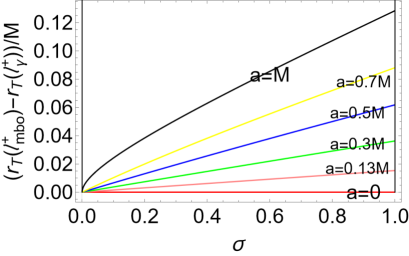
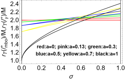
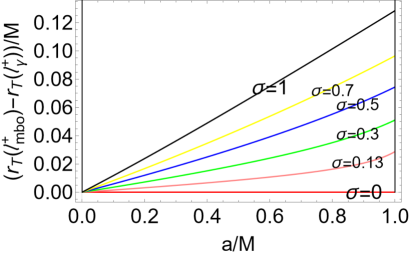
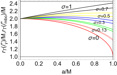
Figure 12: Proto-jets counter-rotating flow turning radius $r_{{\mbox{\scriptsize{{T}}}}}$ evaluated for fluid specific angular momentum $\ell_{mbo}^{+}$ and $\ell_{\gamma}^{+}$ of Eqs (11)). The turning point corona radius $r_{{\mbox{\scriptsize{{T}}}}}(\ell_{mbo}^{+})-r_{{\mbox{\scriptsize{{T}}}}}(\ell_{\gamma}^{+})$ is shown as function of the plane $\sigma\equiv\sin^{2}\theta$ for different BH spin $a/M$ signed on the curve in the upper–left panel and as function of the BH spin $a/M$ for different planes $\sigma$ signed on the curves in the bottom–left panel. Radii $r_{{\mbox{\scriptsize{{T}}}}}(\ell_{mbo}^{+})>r_{{\mbox{\scriptsize{{T}}}}}(\ell_{\gamma}^{+})$ are shown in the upper–right panel as functions of the planes $\sigma$, for different BH spin $a/M$ and as functions of the BH spin $a/M$ for different planes $\sigma$ in the bottom–right panel. The corresponding analysis for the cusped tori counter-rotating driven flows is realized in Figs (5).

In Figs (12) we can compare the counter-rotating proto-jets driven flows corona with Figs (5) for the counter-rotating cusped tori driven flows, completing the analysis of Figs (10). Radius $r_{{\mbox{\scriptsize{{T}}}}}(\ell_{\gamma}^{+})$ is the closest to the ergosurface, making the proto-jets driven corona more internal, i.e. closer to the ergosurface, than the accretion disks driven corona, with a larger spacing between the corona radii and a stronger variation with plane $\sigma_{\mbox{\scriptsize{{T}}}}$ (Figs (12)) and the BH spin (Figs (6)). The proto-jet driven turning point corona is easily distinguishable from the tori driven turning point corona, being located in two separated orbital regions. (It should be noted that Eq. (18) is sufficient to assure that for very small $\sigma$ (i.e. close to the BHs poles) $r_{\mbox{\scriptsize{{T}}}}$ closes on the horizon (in the adopted coordinate frame), as evident also from Figs (10). It is clear that if $\sigma_{\mbox{\scriptsize{{T}}}}\approx 0$, then quantity $\dot{t}_{\mbox{\scriptsize{{T}}}}\to+\infty$, as in Eqs (16), but $\sigma_{\mbox{\scriptsize{{T}}}}$ and $r_{\mbox{\scriptsize{{T}}}}$ are bounded as $r_{\mbox{\scriptsize{{T}}}}>r_{\epsilon}^{+}$.).

6 Verticality of the counter-rotating flow turning point

Consider the vertical flat coordinate $z\equiv r\sqrt{(1-\sigma)}$. Using the coordinate $z_{\mbox{\scriptsize{{T}}}}=r_{\mbox{\scriptsize{{T}}}}\sqrt{(1-\sigma_{\mbox{\scriptsize{{T}}}})}$ for the turning point, there is

$$z_{\mbox{\scriptsize{{T}}}}=r_{\mbox{\scriptsize{{T}}}}\sqrt{\frac{r_{\mbox{\scriptsize{{T}}}}[2a+(r_{\mbox{\scriptsize{{T}}}}-2)\ell]}{a(2r_{\mbox{\scriptsize{{T}}}}-a\ell)}}=\frac{\sqrt{1-\sigma_{\mbox{\scriptsize{{T}}}}}\left[\ell-a\sigma_{\mbox{\scriptsize{{T}}}}-\sqrt{a^{2}\sigma_{\mbox{\scriptsize{{T}}}}^{2}+\ell^{2}\left[a^{2}(\sigma_{\mbox{\scriptsize{{T}}}}-1)+1\right]-2a\sigma_{\mbox{\scriptsize{{T}}}}\ell}\right]}{\ell}$$ (66)

and, for very large $\ell$ in magnitude, $z_{\mbox{\scriptsize{{T}}}}$ tends to the ergosurface $z_{\epsilon}^{+}$ in agreement with Eq. (18).

In agreement with the analysis of Sec. (3.1.3), $z_{\mbox{\scriptsize{{T}}}}$ has no extreme as function of $\ell$, but the vertical coordinate $z_{\mbox{\scriptsize{{T}}}}$ decreases with magnitude of $\ell$ for proto-jet and tori driven counter-rotating flows. Tori corresponding to very large $(-\ell^{+})$ are located far from the attractor (the far the faster spinning is the central BH), and tend to be large and stabilized against the P-W instability, with a consequent regular topology (absence of a torus cusp).

Below we consider $z_{\mbox{\scriptsize{{T}}}}$ as function of the BH $a/M$, the radius $r_{\mbox{\scriptsize{{T}}}}$ and the plane $\sigma_{\mbox{\scriptsize{{T}}}}$, introducing the following spin functions:

$$a_{s}\equiv\frac{\ell+\sqrt{\ell^{2}\left(3\ell^{2}+4\right)}}{2(\ell^{2}+1)},\quad a_{ps}\equiv\frac{\sqrt{(r-2)\left[(r-2)\ell^{2}+4r\right]}-(r-2)\ell}{2},$$ (67)

$$a_{M}\equiv\frac{(5\sigma-2)\ell}{\chi}+2\sqrt{\frac{(1-\sigma)\ell^{2}\left[4(1-\sigma)+3\ell^{2}\right]}{\chi^{2}}}\quad\mbox{where}\quad\chi\equiv(\sigma+2)(3\sigma-2)+4(\sigma-1)\ell^{2}$$ (68)

where spins $a_{s}$ and $a_{M}$ are shown in Figs (13). We also introduce the radii

$$r_{lu}\equiv\frac{{\ell+2}+\sqrt{\ell^{2}-4\ell+8}}{2},\quad r_{+}^{+}\equiv 1+\sqrt{1+a^{2}},\quad r_{ups}\equiv\frac{a\ell+2+\sqrt{a^{2}\left(\ell^{2}+4\right)+4(1-a\ell)}}{2},$$ (69)

$$r_{aps}\equiv\frac{a\left(\ell^{2}-2\right)+\ell\left[\sqrt{\frac{\left[\ell(a\ell-1)+a\right]\left[a\left(\ell^{2}+4\right)-4\ell\right]}{\ell^{2}}}+2\right]}{3\ell},$$ (70)

where $r_{+}^{+}$ and $r_{ups}$ are plotted in Figs (14), while radius $r_{aps}$ and $r_{lu}$, are shown in Figs (13). Furthermore, we define the momenta

$$\ell_{ups}\equiv\frac{r}{a}-\frac{a}{r-2},\quad\ell_{aps}\equiv 2a\left[\frac{1}{4a^{2}-3}-2\sqrt{\frac{1-a^{2}}{\left(4a^{2}-3\right)^{2}}}\right],$$ (71)

$$\ell_{s}\equiv a\left[\frac{(5\sigma-2)}{3-4a^{2}(1-\sigma)}-2\sqrt{\frac{(1-\sigma)\left[a^{2}(\sigma+2)(3\sigma-2)+4(1-\sigma)\right]}{\left[3-4a^{2}(1-\sigma)\right]^{2}}}\right].$$ (72)

Momentum $\ell_{ups}$ is shown in Figs (14), $\ell_{aps}$ is shown in Figs (13) while $\ell_{s}$ is in Figs (16). Finally we consider the planes:

$$\sigma_{s}\equiv\frac{2}{3}\left[\sqrt{\frac{\left[\ell(a\ell-1)+a\right]\left[a\left(\ell^{2}+4\right)-4\ell\right]}{a^{2}}}-\ell^{2}-1\right]+\frac{5\ell}{3a},$$ (73)

$$\sigma_{u}\equiv\frac{\ell(5-2\ell)-2+2\sqrt{(\ell-2)^{2}[(\ell-1)\ell+1]}}{3},\quad\sigma_{e}\equiv\frac{4a^{2}-3}{4a^{2}},$$ (74)

where plane $\sigma_{s}$ is shown in Figs (15) and planes $(\sigma_{e},\sigma_{u})$ are shown in Figs (13).

For $\ell<0$ and $\sigma\in[0,1]$ there are the following extremes for the turning point vertical coordinate $z_{\mbox{\scriptsize{{T}}}}$ as functions of $r$:

$$\partial_{r}z_{\mbox{\scriptsize{{T}}}}=0:\quad\mbox{for}\quad r=r_{aps},\quad\mbox{for}\quad a\in]a_{s},1],$$ (75)

$$\mbox{or alternatively for}\quad a\in\left[\frac{\sqrt{3}}{2},1\right]\quad\mbox{and}\quad\left(a\in\left]0,\frac{\sqrt{3}}{2}\right],\quad\ell\in]\ell_{aps},0[\right).$$ (76)

These results also point out the limiting spin $a/M={\sqrt{3}}/{2}\approx 0.866025$, distinguishing fast rotating from slowly rotating BHs. Radius $r_{aps}$, limiting momentum $\ell_{aps}$ and limiting spin $a_{s}$ are shown in Figs (13).

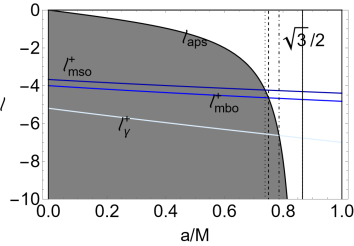
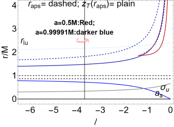
Figure 13: Analysis of the maximum vertical position $z_{\mbox{\scriptsize{{T}}}}$ of the counter-rotating $(\ell<0)$ flow turning point $r_{\mbox{\scriptsize{{T}}}}$ of Sec. (6). There is $z_{\mbox{\scriptsize{{T}}}}=r_{\mbox{\scriptsize{{T}}}}\sqrt{(1-\sigma_{\mbox{\scriptsize{{T}}}})}$, where $\sigma\equiv\sin^{2}\theta$ and $\ell$ is the fluid specific angular momentum. Upper left panel: Limiting plane $\sigma_{e}$ of Eq. (74) as function of the central BH spin-mass ratio $a/M$. Limiting spin $a/M=\sqrt{3}/2$ is shown as dotted line. According to Eq. (83), plane $\sigma_{e}$ constrains the solutions $\partial_{\sigma_{\mbox{\scriptsize{{T}}}}}z_{\mbox{\scriptsize{{T}}}}=0$. Upper right panel: limiting momentum $\ell_{aps}$ of Eq. (71) is plotted as function of the BH spin-mass ratio $a/M$. Momentum $\ell_{aps}$ regulates the analysis of Eqs (76) for the solutions of $\partial_{r}z_{\mbox{\scriptsize{{T}}}}=0$. Limiting momenta $\ell_{mso}^{+}$, $\ell_{mbo}^{+}$ and $\ell_{\gamma}^{+}$, defined in Eqs (11), are also shown. Dotted lines are the limiting conditions for flow, with the specific angular momentum $\ell_{aps}=\{\ell_{mso}^{+},\ell_{mbo}^{+},\ell_{\gamma}^{+}\}$ respectively. Bottom left panel: Limiting plane $\sigma_{u}$ of Eq. (74), radius $r_{aps}$ of Eq. (70) with vertical coordinate $z_{{\mbox{\scriptsize{{T}}}}}(r_{aps})$, limiting spin $a_{s}$ of Eq. (67) and limiting radius $r_{lu}$ of Eqs (69) as functions of fluid specific momenta $\ell$. The situation for the BH spin $a=0.5$ (red curve) and $a=0.99991M$ (darker blue curve) are shown. Radius $r_{lu}$ is a limiting function in the analysis of Eq. (77) for the solutions of $\partial_{a}z_{\mbox{\scriptsize{{T}}}}=0$; spin $a_{s}$ is a limiting function in the analysis of Eqs (75) for the solutions $\partial_{r}z_{\mbox{\scriptsize{{T}}}}=0$, while $\sigma_{u}$ is a limiting plane in the analysis of Eq. (81) for the solutions of $\partial_{\sigma_{\mbox{\scriptsize{{T}}}}}z_{\mbox{\scriptsize{{T}}}}=0$. Bottom right panel shows the limiting plane $\sigma_{u}$ and solution $a=a_{M}$ of Eqs (68) (plain colored curves) in Eq. (81) for solutions of $\partial_{\sigma_{\mbox{\scriptsize{{T}}}}}z_{\mbox{\scriptsize{{T}}}}=0$. Vertical coordinate $z_{\mbox{\scriptsize{{T}}}}(a_{M})$ (dashed-curves) for $\sigma=\sigma_{u}$ (blue curves) and $\sigma=\sigma_{u}/2$ (darker blue curve) are also shown.

Therefore, for $\ell<0$ and $\sigma\in[0,1]$ there are the following extremes of the vertical coordinate $z_{\mbox{\scriptsize{{T}}}}$ with the BH spin–mass ratio:

$$\partial_{a}z_{\mbox{\scriptsize{{T}}}}=0:\quad\mbox{for}\quad a=a_{ps}\quad\mbox{and }\quad r\in]2,r_{lu}],$$ (77)

or equivalently

$$\quad\quad\quad\quad\quad\quad\mbox{for}\quad r=r_{ups}\quad\mbox{and}\quad a\in]0,1],\;$$ (78)

alternatively

$$\quad\quad\quad\quad\quad\quad\mbox{for}\quad\ell=\ell_{ups},\quad\mbox{and}\quad a\in]0,1],\quad r\in]2,r_{+}^{+}[,\quad\mbox{equivalently}$$ (79)

$$\quad\quad\quad\quad\quad\quad\mbox{for}\quad\ell=\ell_{ups},\quad\mbox{and }\quad a\in]a_{\pm},1],\quad r/M\in]2,\sqrt{2}+1[,$$ (80)

where $a_{\pm}\equiv\sqrt{r(2M-r)}$ is the horizons curve in the plane $a-r$. It is immediate to see that the radius $r=r_{\mbox{\scriptsize{{T}}}}$ is upper bounded by the limiting value $r_{\mbox{\scriptsize{{T}}}}=(\sqrt{2}+1)M=2.41421M$, according to the analysis Sec. (3.1.1) and Eq. (44). (There is $z_{\mbox{\scriptsize{{T}}}}(\ell_{ups})=r\sqrt{{(r-2M)r}/{a^{2}}}$, Figs (14), while the ergoregion is $z_{\epsilon}^{+}=r\sqrt{{(2M-r)r}/{a^{2}}}=r(a_{\pm}/a)$). Limiting radius $r_{lu}$ is shown in Figs (13), momentum $\ell_{ups}$, radius $r_{ups}$, vertical momentum $z_{\mbox{\scriptsize{{T}}}}(r_{ups})$ and limiting radius $r_{+}^{+}$ are shown in Figs (14). There is $z_{{\mbox{\scriptsize{{T}}}}}(r_{ups})<1.77M$, decreasing with the increase of the dimensionless spin $a/M$.

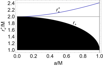
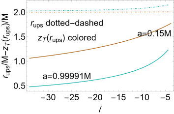
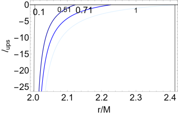
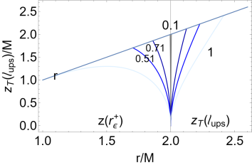
Figure 14: Analysis of the maximum vertical position of the counter-rotating flow turning point of Sec. (6). There is $z_{\mbox{\scriptsize{{T}}}}=r_{\mbox{\scriptsize{{T}}}}\sqrt{(1-\sigma_{\mbox{\scriptsize{{T}}}})}$. Upper left panel: black region is the central BH with $r<r_{+}$, where $r_{+}$ is the BH horizon. Radius $r_{+}^{+}$ of Eq. (69), is plotted as function of the BH spin–mass ratio $a/M$, considered in the analysis of Eq. (79), governing the solutions of $\partial_{a}z_{\sigma_{\mbox{\scriptsize{{T}}}}}=0$. Right upper panel: radii $r_{ups}$ of Eq. (69), (dotted-dashed curves), maximum vertical coordinate of the counter-rotating flow turning point, solution of $\partial_{a}z_{\sigma_{\mbox{\scriptsize{{T}}}}}=0$ and the vertical coordinate $z_{\mbox{\scriptsize{{T}}}}(r_{ups})$ (colored curves) as functions of the fluid specific angular momentum $\ell$, for spin $a=0.15M$ (red curves) $a=0.99991M$ (darker-cyan curve)–see analysis of Eq. (78). Below panels: specific momenta $\ell_{ups}$ of Eqs (71) (left panel) as function of the radial distance from the attractor $r/M$ and the vertical coordinate of the turning point $z_{\mbox{\scriptsize{{T}}}}(\ell_{ups})$ as function of $r/M$ (right panel) for different BH spin-mass ratios $a/M$ signed on the curves. In the right panel the ergosurface vertical coordinate $z(r_{\epsilon}^{+})$ is also shown, see analysis of Eqs (79) and (80).

For $\ell<0$, the extremes of $z_{\mbox{\scriptsize{{T}}}}$ according to the plane $\sigma$ are

$$\partial_{\sigma_{\mbox{\scriptsize{{T}}}}}z_{\mbox{\scriptsize{{T}}}}=0:\quad\mbox{for}\quad\left(\sigma\in[0,\sigma_{u}],\;a=a_{M}\right),\quad\mbox{or equivalently}$$ (81)

$$\quad\quad\quad\mbox{for}\quad\left(\sigma=\sigma_{s},a\in]a_{s},1]\right);\quad\left(a=a_{s},\;\sigma=0\right),$$ (82)

or alternately

$$\mbox{for}\quad\ell=\ell_{s}:\quad\mbox{and}\quad\left(a\in\left]0,\frac{\sqrt{3}}{2}\right[,\;\sigma\in\left[0,\frac{2}{3}\right[\right);\;\left(a=\frac{\sqrt{3}}{2},\;\sigma\in\left]0,\frac{2}{3}\right[\right);\left(a\in\left]\frac{\sqrt{3}}{2},1\right],\;\sigma\in\left]\sigma_{e},\frac{2}{3}\right[\right).$$ (83)

Solution $\ell_{s}$ is shown in Figs (16). Limiting plane $\sigma_{e}$ and solution $a_{M}$ are shown in Figs (13). Plane $\sigma_{s}$ is in Figs (15). In this analysis we single out the limiting critical plane $\sigma=2/3\approx 0.666667$ and spin $a/M=\sqrt{3}/2$, showing the different situation for slowly spinning attractors and fast attractors, and turning points closer or farer from the BH poles. We can note the different situations for the counter-rotating flows from the cusped tori and proto-jets driven flows. Considering Figs (15), there is $a\geq 0.74M$ and $\sigma_{s}<0.35$, with $\sigma_{s}$ increasing with the spin and $z_{\mbox{\scriptsize{{T}}}}<1.75M$ (generally) decreasing with the spin $a/M$. There exists a discriminant spin $a\approx 0.77M$. For slower spin $a/M$, the vertical coordinate turning point is higher for the proto-jet driven flow than for cusped tori flow. For larger BH spins, the situation is inverted and the regions for turning points in proto-jets driven flows spread, according to the different planes and decrease with increasing BH spin.

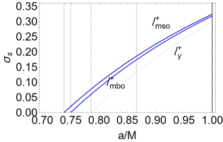
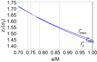
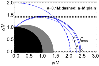
Figure 15: Left panel: maximum plane $\sigma_{s}$ of Eq. (73), for fluid specific momenta $\ell_{mso}^{+}$, $\ell_{mbo}^{+}$ and $\ell_{\gamma}^{+}$, defined in Eqs (11), signed on the curves. Center panel: the maximum vertical coordinate of the turning point of the counter-rotating flow as function of the spin-mass ratio of the central BH (solutions of $\partial_{\sigma_{\mbox{\scriptsize{{T}}}}}z_{\mbox{\scriptsize{{T}}}}=0$) of Eq. (82). Dotted lines are the limiting condition for $\sigma=0$ (BH poles) on $\ell_{mso}^{+}$, $\ell_{mbo}^{+}$ and $\ell_{\gamma}^{+}$. There is $z_{\mbox{\scriptsize{{T}}}}=r_{\mbox{\scriptsize{{T}}}}\sqrt{(1-\sigma_{\mbox{\scriptsize{{T}}}})}$, where $\sigma\equiv\sin^{2}\theta$–see Sec. (6).Right panel: analysis of the turning sphere maximum vertical point $z_{\mbox{\scriptsize{{T}}}}$. Black region is the BH $r<r_{+}$ (with outer horizon $r_{+}$), gray region is $r\in]r_{+},r_{\epsilon}^{+}]$, where $r_{\epsilon}^{+}$ is the outer ergosurface. Dashed (plain) curves are the turning spheres for $a=0.1M$ ($a=M$).

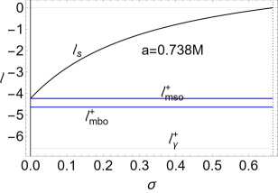
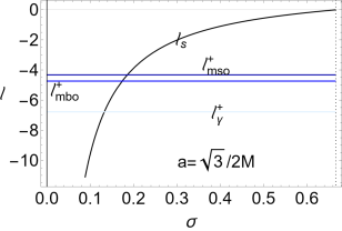
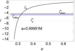
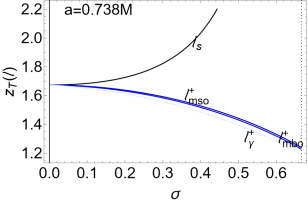
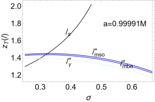
Figure 16: Analysis of the maximum vertical position $z_{\mbox{\scriptsize{{T}}}}=r_{\mbox{\scriptsize{{T}}}}\sqrt{(1-\sigma_{\mbox{\scriptsize{{T}}}})}$ of the counter-rotating flow turning point of Sec. (6). Fluid specific angular momentum, $\ell_{s}$ of Eqs (72) (upper panels) and vertical coordinate of the turning point $z_{{\mbox{\scriptsize{{T}}}}}(\ell)$ (bottom panels) evaluated on $\ell_{s}$ and for momenta $\ell_{mso}^{+}$, $\ell_{mbo}^{+}$ and $\ell_{\gamma}^{+}$ defined in Eqs (11) signed on the curves are plotted as functions of the plane $\sigma\equiv\sin^{2}\theta$. Different BH spins $a/M$, signed on the panels are considered. Momentum $\ell_{s}$ is solution of $\partial_{\sigma_{\mbox{\scriptsize{{T}}}}}z_{\mbox{\scriptsize{{T}}}}=0$–see Eq (83).

The turning point therefore is not a characteristic of the matter funnels or photons jets structures, collimated along the BH axis, but remains a defined vertical structure in a cocoon surrounding the ergosurface and closing on the outer ergosurface $r_{\epsilon}^{+}$, more internal with respect to the tori driven flows turning corona. This aspect was also partially dealt with in Sec. (3.1.2), in relation to the analysis of Figs (10) for the double turning points at fixed $(\ell,z)$. The presence of a vertical maximum is an indication of the double turning point on the vertical axi. Constrained by the condition $z_{\mbox{\scriptsize{{T}}}}=r_{+}$ at $y_{\mbox{\scriptsize{{T}}}}(+)>0$, double turning points are possible for fast spinning BHs, e.g., with $a>0.74$ for fluids with $\ell=\ell_{mso}^{+}$, and $a>0.75$ for fluids with $\ell=\ell_{mbo}^{+}$. Here we specify these results regarding the presence of the maximum. In Figs (15) is the analysis of the vertical maximum ($\partial_{y}{{}_{\mbox{\scriptsize{{T}}}}}z_{\mbox{\scriptsize{{T}}}}=0$) for different BH spins $a/M$ and momenta $\ell<0$. The maximum increases, decreasing the BH spin with the limiting situation of $a\geq 0$ and $z_{\mbox{\scriptsize{{T}}}}\leq 2M$. Then it is maximum at $\ell_{mso}^{+}$ (decreases with the magnitude of $\ell$), and the bottom boundary of the maximum $z_{\mbox{\scriptsize{{T}}}}$ occurs for the extreme BH with $a=M$. Then, at $a=M$ there is the maximum $z^{\max}_{\mbox{\scriptsize{{T}}}}=1.451M$ for $\ell=\ell_{mso}^{+}$, $z^{\max}_{\mbox{\scriptsize{{T}}}}=1.437M$ for $\ell=\ell_{mbo}^{+}$, and $z^{\max}_{\mbox{\scriptsize{{T}}}}=1.39M$ for $\ell=\ell_{mso}^{+}$.

7 Flow thickness and counter-rotating tori energetics

For the tori and proto-jets counter-rotating driven flows turning point, is located at $r>r_{\epsilon}^{+}$ .

However we can study the frame–dragging influence on the accretion flow from the counter-rotating tori considering the flow thickness of the super-critical tori (with $K=K_{s}\in]K_{\times},1[$) throats. We start by analyzing the thickness of the accretion flow in the counter-rotating configurations. (A comparative analysis with the corotating flows can be found for example in Pugliese&Stuchlik (2018a, 2017b, b)).

According to the analysis in Abramowicz (1985)–see also Pugliese&Stuchlik (2018b, 2017b, a)–we can relate some energetic characteristics of the orbiting disks to the thickness of the super-critical tori flows (with $K=K_{s}\in]K_{\times},1[$ for accretion driven flows). Considering polytropic fluids, at the inner edge (cusp) the flow is essentially pressure-free. To consider all possible cases, we fix the cusp location, the throat thickness and location, fluid momenta $\ell=\ell_{ecc}$ and $K=K_{s}$ parameter according to the following definitions:

$$K_{s}(\xi,\ell;a)\equiv K_{\times}+\frac{1-K_{\times}}{\xi},\quad\ell_{ecc}(\psi;a)\equiv\ell_{mso}^{+}+\frac{\ell_{mbo}^{+}-\ell_{mso}^{+}}{\psi},\quad\mbox{where}\quad K_{\times}(\ell;a)=K(r_{\times}),$$ (84)

where $r_{\times}$ is in Eqs (10) and $(\xi,\psi)$ are two positive constants regulating the momentum $\ell$ and the $K$ parameter in the accretion driven range of values–Figs (17), with

$$\xi\in[1,+\infty],\quad\psi\in[1,+\infty],\quad\lim\limits_{\xi\rightarrow 1}K_{s}=1,\quad\lim\limits_{\xi\rightarrow+\infty}K_{s}=K_{\times},\quad\lim\limits_{\psi\rightarrow 1}\ell_{ecc}=\ell_{mbo}^{+},\quad\lim\limits_{\psi\rightarrow+\infty}\ell_{ecc}=\ell_{mso}^{+}.$$

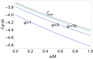
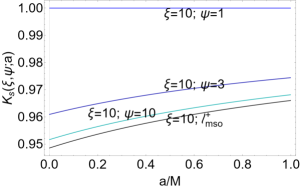
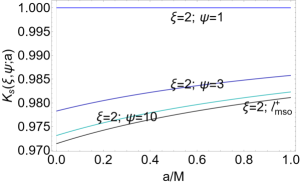
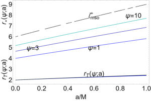
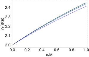
Figure 17: Upper left panel counter-rotating fluid specific angular momentum $\ell_{ecc}(\psi;a)$ of Eq. (84) for different values of $\psi:\ell\in[\ell_{mbo}^{+},\ell_{mso}^{+}]$ for the maximum extension of the turning corona. Limiting fluid specific momenta $\ell_{mso}^{+}$ and $\ell_{mbo}^{+}$ are defined in Eqs (11). Central and right upper panels: quantities $K_{s}\in[K_{\times},1]$, regulating the flux thickness of Eq. (84) for different values of $\psi$ signed on the curves for $\xi=10$ (central panel) and $\xi=2$ (right panel). Bottom left panel: parameter $K$ evaluated at the torus cusp for different values of the momenta parameter $\psi$ signed on the curves. Center bottom panel: cusp location $r_{\times}$ for different values of $\psi$ and correspondent turning point location $r_{\mbox{\scriptsize{{T}}}}$. Bottom right panel shows a zoom of the $r_{\mbox{\scriptsize{{T}}}}$ for different values of $\psi$ according to the color choice of the central panel.

(However in the range $\psi\in[0,1[$, momenta $\ell_{ecc}(\psi)$ describe proto-jet driven flows where $\ell\in\mathbf{L_{2}}$, or tori with $\ell\in\mathbf{L_{3}}$). The limiting value of $\psi$ in this case is $\psi_{\gamma}\equiv({\ell_{mbo}^{+}-\ell_{mso}^{+}})/({\ell_{\gamma}^{+}-\ell_{mso}^{+}})$, which is a function of $a/M$–Fig. (18).

While $r_{\times}$ is the cusp location fixed by $\ell=\ell_{ecc}$, radius $r_{s}<r_{\times}$ is related to the accreting matter flow thickness and determined by the parameter $K_{s}$–see Figs (17).

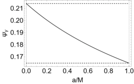
Figure 18: Parameter $\psi_{\gamma}:\ell_{ecc}=\ell_{\gamma}^{+}$ as function of the BH spin-mass ratio $a/M$. Counter-rotating fluid specific angular momentum $\ell_{ecc}(\psi;a)$ is defined in Eq. (84), there is $\ell_{\gamma}^{+}=\ell(r_{\gamma}^{+})$ where $r^{+}_{\gamma}$ is the counter-rotating photon last circular orbit.

Consider counter-rotating tori with pressure $p=\kappa\varrho^{1+1/n}$, where $\gamma\equiv 1+1/n$ is the polytropic index and $\kappa$ is a polytropic constant. The mass-flux, the enthalpy-flux (related to the temperature parameter), and the flux thickness can be estimated as $\Gamma$–quantities, having general form $\Gamma(r_{\times},r_{s},n)=\beta_{1}(n,\kappa)(W_{s}-W_{\times})^{\beta_{2}(n)}$, where $\{\beta_{1}(n,\kappa),\beta_{2}(n)\}$ are functions of the polytropic index and constant and $W=\ln K$. (More specifically the $\Gamma$–quantities are: the $\mathrm{{{Enthalpy-flux}}}=\mathcal{D}(n,\kappa)(W_{s}-W)^{n+3/2}$; the $\mathrm{{{Mass-Flux}}}=\mathcal{C}(n,,\kappa)(W_{s}-W)^{n+1/2}$ and the $\mathcal{\bar{L}}_{\times}/\mathcal{\bar{L}}=\mathcal{B}/\mathcal{A}(W_{s}-W_{\times})/(\eta c^{2})$, which is the fraction of energy produced inside the flow and not radiated through the surface but swallowed by central BH. While $\mathcal{\bar{L}}$ is the total luminosity, and $(\mathcal{D}(n,\kappa),\mathcal{C}(n,\kappa),\mathcal{A}(n,\kappa),\mathcal{B}(n,\kappa))$ are functions of the polytropic index and polytropic constant, $\dot{M}$ is the total accretion rate where, for a stationary flows, $\dot{M}=\dot{M}_{\times}$ and $\eta\equiv\mathcal{L}/\dot{M}c^{2}$ is the efficiency.)

We examine also the $\delta$-quantities, having general form $\delta={\Gamma}(r_{\times},r_{s},n)r_{\times}/\Omega(r_{\times})$; where $\Omega(r_{\times})$ is the relativistic angular frequency at the tori cusp $r_{\times}$ where the pressure vanishes. The $\delta$-quantities regulate the cusp luminosity, measuring the rate of the thermal-energy carried at the cusp, the disk accretion rate, and the mass flow rate through the cusp (i.e., mass loss accretion rate). (More specifically, the $\delta$–quantities are: the cusp luminosity $\mathcal{L}_{\times}={\mathcal{B}(n,K)r_{\times}(W_{s}-W_{\times})^{n+2}}/{\Omega(r_{\times})}$, the disk accretion rate $\dot{m}=\dot{M}/\dot{M}_{Edd}$ (compared to the characteristic Eddington accretion rate); the mass flow rate through the cusp $\dot{M}_{\times}={\mathcal{A}(n,K)r_{\times}(W_{s}-W_{\times})^{n+1}}/{\Omega(r_{\times})}$, where $(\mathcal{A}(n,\kappa),\mathcal{B}(n,\kappa))$ are functions of the polytropic index and polytropic constant.). In the analysis of Figs (19) we assumed $\beta_{1}=\beta_{2}=1$. It is clear that these quantities, depending on the details of the toroidal models, provide a wide estimation for more refined tori models. Nevertheless with this analysis these quantities can be estimated in relation with fluid thickness (regulated by $W_{s}-W_{\times}$), the tori distance from the central attractor (cusp location $r_{\times}\in[r_{mbo}^{+},r_{mso}^{+}]$ fixing also the center of maximum density and pressure in the disk) and the BH spin.

The toroidal models used in this analysis are shown in Figs (17) in terms of $\ell_{ecc}$, cusp location $r_{\times}$, the flow turning radius $r_{\mbox{\scriptsize{{T}}}}$, and parameter values $K_{s}$ and $K_{\times}$.

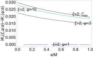
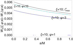
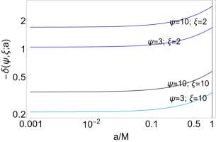
Figure 19: Difference $W_{s}-W_{\times}$, defining the $\Gamma$–quantities introduced in Sec. (7), where $W\equiv\ln K$ for $\xi=2$ (left panel) and $\xi=10$ (center panel) are shown as functions of the BH spin-mass ratio $a/M$, at different fluid momenta $\ell$ regulated by the $\psi$ parameters signed on the curves–see Eq. (84). The $\Gamma$–quantities regulate the mass–flux, the enthalpy–flux (related to the temperature parameter), and the flux thickness. Right panel: $\delta$–quantities (regulating the cusp luminosity, measuring the rate of the thermal–energy carried at the cusp, the disk accretion rate, and the mass flow rate through the cusp i.e., mass loss accretion rate) defined in Sec. (7) are shown for different values of $\psi$ (regulating the momenta) and $\xi$ (regulating $K_{s}\in]K_{\times},1[$) signed on the curves.

As clear from Figs (17) and Figs (19), the $\Gamma$–quantities decrease with the BH spin $a/M$, with decreasing $K_{s}\in]K_{\times},1[$, and decrease with increasing $\ell\in]\ell_{mbo}^{+},\ell_{mso}^{+}]$ in magnitude. The $\delta$–quantities increase with the BH spin mass ratio, with increasing $K$ and with the decrease of $\ell$ in magnitude. For greater values of $\Gamma$– and $\delta$–quantities, the flow thickness, regulated by the $K$ parameter (larger values of $(K_{s}-K_{\times})$ correspond to larger flow thickness) is mostly dependent on the background properties, especially for fast spinning attractors. (For fast spinning attractors the flow thickness is in fact largely independent on the tori details and properties). Furthermore, for the counter-rotating flows, the closer to the BH the tori are (smaller magnitude of the $\ell$) the greater $\Gamma$– and $\delta$–quantities are. The counter-rotating tori energetics are mostly dependent from the characteristics of the accreting tori for slowly spinning attractors (where similarities are with the corotating tori), which are closer to the attractor and with smaller magnitude of momenta (note that the flow reaches the central attractor with negative $\ell$ and, on each trajectory, there could also be two turning points).

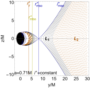
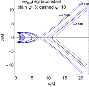
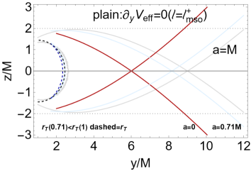
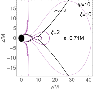
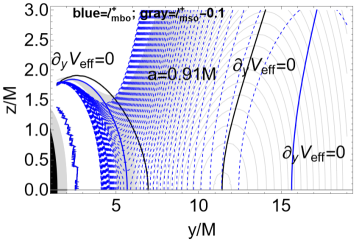
Figure 20: Tori models: equidensity surfaces and surfaces of constant $\ell$, related to the analysis of Sec. (7). Black region is the central BH, gray region is the outer ergoregion, there is $r=\sqrt{z^{2}+y^{2}}$ and $\sigma=(\sin\theta)^{2}={y^{2}}/({z^{2}+y^{2}})$, and $\ell$ is the fluid specific angular momentum. Upper left panel: solutions of equation $\ell^{+}=\partial_{y}V_{eff}(a;y,z,\ell)=0$, coincident with $\ell^{+}(x,y,a)=$constant are shown in the BH spacetime with spin $a=0.71M$. Momenta $\ell$ are in the range $\mathbf{L_{2}^{+}}\equiv[\ell_{\gamma}^{+},\ell_{mbo}^{+}]$, for counter-rotating proto-jets driven flows (dotted–dashed dark– yellow curves), and range $\mathbf{L_{1}^{+}}\equiv[\ell_{mbo}^{+},\ell_{mso}^{+}]$, for counter-rotating cusped tori driven flows (dashed black curves). Momenta and geodesic radii shown in the panels are defined in Eqs (11). Curves connect the center of maximum density and pressure with the tori geometrical maxima in the range $y=r>r_{mso}^{+}$, and the cusp $r_{\times}$ (minimum of pressure), fixed by momentum $\ell^{+}=$constant with the minima of the matter throat $(K>K_{\times})$, providing thus indication of tori (and matter throat) thickness. Central upper panel shows the curves $\ell=$constant for different BH spins $a/M$ signed on the curves and for momenta $\ell_{ecc}$ with $\psi=3$ and $\psi=10$ of Eq. (84). Right upper panel: limiting counter-rotating solutions for $\ell=\ell_{mso}^{+}$, in the BH spacetimes $a=0$ (Schwarzschild), $a=0.71M$ and $a=M$ (extreme Kerr BH), and the related turning radius $r_{\mbox{\scriptsize{{T}}}}(\sigma)$, plotted as inner dashed curves. Below panels: cusped and super–critical tori at $\psi=3$ (left) and $\psi=10$ (center), where $\psi$ fixes the fluid momenta $\ell_{ecc}$, and different $\xi$ signed on the curves ($\xi$ fixes the $K_{s}$ parameter) of Eq. (84). Black curves are solutions of $\ell^{+}(y,z,a)=$constant. Right panel: toroidal surfaces in the BH spacetimes $a=0.91M$ at $\ell=(\ell_{mso}^{+}-0.1)$(gray line) and $\ell_{mbo}^{+}$ (blue-dashed lines). Blue and black plain lines are curves $\ell(x,y,z):\partial_{y}V_{eff}=0$ constant.

Maximum density and pressure points and tori thickness

Introducing the coordinates $(y,z):r=\sqrt{y^{2}+z^{2}}$ and $\sigma=(\sin\theta)^{2}={y^{2}}/({z^{2}+y^{2}})$, solutions of $\ell^{+}=\partial_{y}V_{eff}(a;z,y,\ell)=0$, coincident with solutions of $\ell^{+}(x,y,a)=$constant, shown in Figs (20), are the curves connecting the center of maximum density and pressure for barotropic fluids (uniquely fixed by the $\ell$ parameter) with the tori geometrical maxima (regulating the tori thickness and fixed by $K$) in the range $y=r>r_{mso}^{+}$ for cusped tori, and the curve connecting the cusp $r_{\times}$ (minimum of pressure, uniquely fixed by the $\ell$ parameter), with the extremes of the flow throat (regulating the flow thickness and fixed by $K$), and therefore provides the throat thickness for super-critical tori–Figs (20). Therefore, the throat thickness, similarly to the turning point function $r_{\mbox{\scriptsize{{T}}}}(\sigma_{\mbox{\scriptsize{{T}}}})$, is governed by the fluid specific angular momentum.

The maximum thickness of the accretion throat

More specifically, solution $\ell(x,y,z):\partial_{y}V_{eff}=0$ provides, for fixed $a/M$, the curve $\mathcal{C}^{+}_{\ell^{+}}$, representing the torus center, i.e. maximum of fluid pressure (on $z=0$), and torus geometrical maximum (on $z>0$), at $r>r_{center}$, for any $K\geq K_{center}$ and, at $y=r<r_{inner}$ (torus inner edge) the curve $\mathcal{C}^{-}_{\ell^{+}}$, containing the minimum of fluid pressure (on $z=0$), i.e. torus cusp $r_{\times}$ or proto-jets cusp $r_{j}$, and the geometrical minimum (on $z>0$) of the throw boundary (region $y<r_{\times}$) for the over-critical tori ($K>K_{\times}$). Therefore curve $\mathcal{C}^{-}_{\ell^{+}}$ provides in this sense a definition of throat thickness–see Figs (20)-below panels, while it is clear that the Roche lobe generally increases with $\ell$. The analysis of Fig. (20)-upper left panel shows, for $y<r_{inner}$ that the higher $\mathcal{C}^{-}_{\ell}$ curve (larger throat thickness) is, at fixed $a/M$, for the curve $\mathcal{C}^{-}_{\ell_{mso}^{+}}$ defined by momentum $\ell=\ell_{mso}^{+}$. For $|\ell^{+}|>|\ell_{mso}^{+}|$, curves $\mathcal{C}^{-}_{\ell}$ are upper bounded by the curve $\mathcal{C}^{+}_{\ell_{mso}^{+}}$, at $\ell=\ell_{mso}^{+}$, which is also the more extended on the equatorial plane (cusp located far on the equatorial plane). Fig. (20)-upper center and right panel show that in this sense the throat thickness increases with the BH spin (increasing the BH spin $a/M$, the curves $\mathcal{C}^{-}_{\ell^{+}}$ (at $\ell(x,y,z)=$constant) stretch far from the central attractor with $y=r_{mso}^{+}$ (cusp of the curve at $\ell_{mso}^{+}$).).

As shown in Figs (20), the maximum thickness of the flow throat for super-critical tori is provided by the limiting solution with $\ell^{+}=\ell_{mso}^{+}$, and therefore determined only by the background properties through BH dimensionless spin. The maximum accretion throat thickness increases with the BH spin $a/M$, reaching its maximum at $a=M$. As the cusp moves outwardly on the equatorial plane $(z=0)$ with increasing BH spin (and tori angular momentum magnitude), the counter-rotating flow throat extends on the equatorial plane. The turning points $r_{\mbox{\scriptsize{{T}}}}$ is a bottom limit of the throat as shown in Figs (20)–(upper-right-panel), with $\ell_{mso}^{+}$ being also the outer boundary of the turning corona.

Although the counter-rotating orbiting tori may be also very large, especially at large BH spins, the momentum is limited in $\mathbf{L_{1}}$ and the width of the throat, dependent only on $K_{\times}-1$, seen in Figs (17) remains very small and included in a region whose vertical coordinate $z_{throat}\in[-2M,2M]$ and generally $z_{throat}>z_{\mbox{\scriptsize{{T}}}}$. Therefore the BH energetics would depend on its spin $a/M$ (as the tori energetics essentially depends on the BH spin) rather than on the properties of the counter-rotating fluids or the tori masses–Figs (19). The fluid contributes to the BH characteristic parameters (spin $J$, total mass $M$ and then rotational mass $M_{rot}$(Pugliese&Stuchlik, 2021a)), with matter of momentum $\ell<0:\ell\in]\ell_{mbo}^{+},\ell_{mso}^{+}[$, for the matter swallowed by the attractor, having a turning point far from the ergosurface and the accretion throat–Figs (19). This implies also that the maximum amount of matter swallowed by the BH from the counter-rotating tori considered here is constrained by the limiting configurations with $\ell=\ell_{mso}^{+}$.

8 On the fluids at the turning point

In Figs (3) we show the flow from a counter-rotating torus with a turning point on the equatorial plane, however the fluid particles trajectories at $\tau>\tau_{\mbox{\scriptsize{{T}}}}$ ($t>t_{\mbox{\scriptsize{{T}}}}$) depend on the fluid initial data. In this section we analyze the flow particles accelerations $\dot{u}_{{\mbox{\scriptsize{{T}}}}}$ at the turning point. To simplify the discussion we limit the analysis to matter particles ($\mu=1$) at the turning point on the equatorial plane, where $\mathcal{Q}=0$, $\theta_{\mbox{\scriptsize{{T}}}}=\pi/2$ and $\dot{\theta}_{\mbox{\scriptsize{{T}}}}=\ddot{\theta}_{\mbox{\scriptsize{{T}}}}=0$, and using the second-order differential equations of the geodesic motion within the constrain provided by the normalization condition. Tori models for the counter-rotating flows are defined by the function $\ell=\ell_{ecc}(\psi,a)$ of Eq. (84), using the condition $\ell_{ecc}=\mathcal{L}/\mathcal{E}$ where $\mathcal{E}\equiv K(r_{\times})$ and $r_{\times}$ is given by Eq. (10), and by using the turning point radius $r=r_{\mbox{\scriptsize{{T}}}}^{e}$ for outgoing/ingoing particles defined by $\dot{r}_{\mbox{\scriptsize{{T}}}}\gtrless 0$ respectively– Figs (21). (The radial acceleration is independent from the radial velocity sign as the dependence from the even power of $\dot{r}$ depends on $\dot{\theta}_{\mbox{\scriptsize{{T}}}}$ which, in the case considered here, is zero).

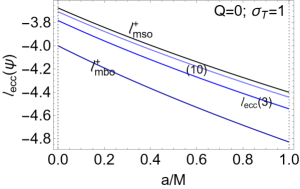
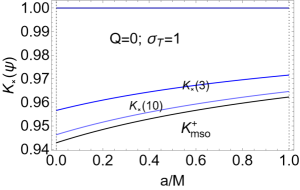
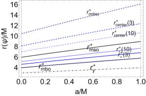
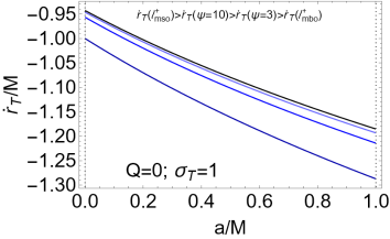
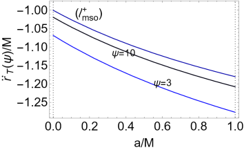
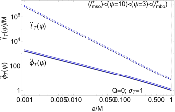
Figure 21: Analysis of the ingoing particles ($\dot{r}_{\mbox{\scriptsize{{T}}}}<0$) at the tori driven counter-rotating fluid turning point on the equatorial plane $\sigma_{\mbox{\scriptsize{{T}}}}=1$ ($\sigma\equiv\sin^{2}\theta$), with Carter constant $\mathcal{Q}=0$ and $\dot{\theta}=\ddot{\theta}=0$. Upper panels: tori models fixing the initial data for the infalling counter-rotating flows. Upper–left panel: fluid angular momentum Eq. (84), functions of the BH spin-mass ratio $a/M$, for different values of the parameter $\psi$. Momenta $\ell_{mso}^{+}$, $\ell_{mbo}^{+}$ and $\ell_{\gamma}^{+}$ and radii $r_{mso}^{+}$, $r_{mbo}^{+}$, $r_{(mbo)}^{+}$ and $r_{\gamma}^{+}$ defining the turning corona boundaries are defined in Eqs (11). Upper center panel: cusped tori energy parameter $K$ evaluated at the cusp $r_{\times}$ of the counter-rotating torus, for different values of the fluid specific angular momentum parameter $\psi$ signed on the curves.Upper-right panel: tori cusp location $r_{\times}$ and center $r_{center}$ as functions of the BH spin $a/M$, for different fluid angular momenta $\ell_{ecc}$. Center line panels: time velocity component $\dot{t}_{\mbox{\scriptsize{{T}}}}$ (left panel) and radial component $\dot{r}_{\mbox{\scriptsize{{T}}}}$ (right panel) at the turning point of Eq. (38), functions of the BH spin $a/M$ for different momenta $\ell_{ecc}$. Below line panels: fluid acceleration $\ddot{r}_{\mbox{\scriptsize{{T}}}}$ (left panel) and $\ddot{t}_{\mbox{\scriptsize{{T}}}},\ddot{\phi}_{\mbox{\scriptsize{{T}}}}$ (right panel) at the turning point, functions of the BH spin $a/M$ for different $\ell_{ecc}$.

In fact, as already mentioned, the turning coronas are a background property, depended only on the BH dimensionless spin $a/M$. Each turning sphere depends on the specific angular momentum $\ell$, indifferently for ingoing or outgoing particles or with other velocity components at the turning point, for example with motion along the vertical axis, therefore here we complete this analysis considering the general frame where there can be particles and photons with an outgoing radial component of the velocity.

The central BH is not isolated and there will be matter, and photons radiated in any direction, the eventual turning points of the general trajectories will be located on the turning spheres, equal for photons and particles. The analysis of Figs (21),(22), (23), (24) gives us an indication on the trajectories crossing the turning sphere, connected with the tori parameters fixed in the study of the tori energetics. We also considered counter-rotating photons for comparison with the infalling matter. We fix the velocities and accelerations at the flow turning point for fixed toroidal cusped models of Eq. (84) ($\psi=$constant) to describe the situation with variation of the BH spin and the fluid specific angular momentum $\ell\in\mathbf{L_{1}}$. We also show the tori inner parts in different tori models. We can note how $\dot{t}_{\mbox{\scriptsize{{T}}}}$ decreases with the spin $a/M$ and the momenta $\ell$ in magnitude, while the radial (infalling) velocity increases in magnitude with the spin (distinguishing fast spinning from slowly spinning attractors) and increases with the decreasing momenta in magnitude. The analysis of the toroidal acceleration defines $\phi_{\mbox{\scriptsize{{T}}}}$ as extreme of the $\phi(\tau)$, as for assumption there is $\dot{\phi}_{\mbox{\scriptsize{{T}}}}\lesseqgtr 0$ for $\tau\lesseqqgtr\tau_{\mbox{\scriptsize{{T}}}}$ respectively. As there is $\ddot{\phi}_{\mbox{\scriptsize{{T}}}}(\tau)>0$, the derivative $\dot{\phi}(\tau)$ increases.

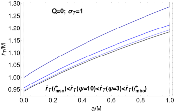
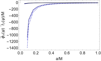
Figure 22: Tori driven counter-rotating flow particles accelerations $(\ddot{\phi}_{\mbox{\scriptsize{{T}}}},\ddot{t}_{\mbox{\scriptsize{{T}}}})$ (right panel) and radial velocity $\dot{r}_{\mbox{\scriptsize{{T}}}}$ (left panel) at the fluid turning point on the equatorial plane $\sigma_{\mbox{\scriptsize{{T}}}}=1$ (where $\sigma\equiv\sin^{2}\theta$), with Carter constant $\mathcal{Q}=0$ and $\dot{\theta}=\ddot{\theta}=0$, for outgoing particles $\dot{r}_{\mbox{\scriptsize{{T}}}}>0$ from the toroidal models of Figs (21). Velocity $\dot{r}_{\mbox{\scriptsize{{T}}}}$ and accelerations $(\ddot{\phi}_{\mbox{\scriptsize{{T}}}},\ddot{t}_{\mbox{\scriptsize{{T}}}})$ differentiate outgoing particles from the ingoing particles cases of Figs (21).

To complete the analysis we also consider the outgoing condition in Figs (22) and the case of photons in Figs (23)—see also Figs (24)–

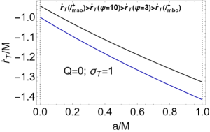
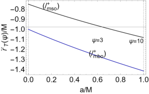
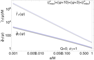
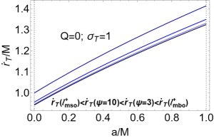
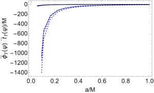
Figure 23: Accelerations components and radial velocities at the tori-driven counter-rotating fluid turning point on the equatorial plane $\sigma_{\mbox{\scriptsize{{T}}}}=1$, where $\sigma\equiv\sin^{2}\theta$, with Carter constant $\mathcal{Q}=0$ and $\dot{\theta}=\ddot{\theta}=0$, for ingoing (upper panels) and outgoing (below panels) photons for the toroidal models of Figs (21).

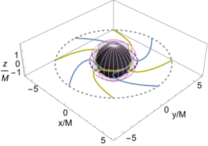
Figure 24: Tori driven counter-rotating flows photons turning points in the BH spacetime with spin-mass ratio $a/M=0.71$ of the cusped tori of Figs (3). The torus has fluid specific angular momentum $\ell=-4.5$, where is $\{z=r\cos\theta,y=r\sin\theta\sin\phi,x=r\sin\theta\cos\phi\}$ in dimensionless units. The limiting fluid specific angular momenta, defined in Eqs (11), are $\{\ell_{mso}^{+}=-4.21319,\ell_{mbo}^{+}=-4.61534,\ell_{\gamma}^{+}=-6.50767\}$. The cusped torus is orbiting the equatorial plane of the central BH. Left and right panels show a front and above view of the counter-rotating flow stream from the torus inner edge (cusp-dashed gray curve) to the central BH. Black region is the central BH (region $r<r_{+}$, radius $r_{+}$ is the outer horizon). Flow turning point $r_{{\mbox{\scriptsize{{T}}}}}=2.31556M$ of Eqs (15),(19), (42) is plotted as the deep-purple curve. The initial radial velocity normalization conditions for photons have been used to find $\dot{r}_{0}$. Radius $r_{{\mbox{\scriptsize{{T}}}}}$ lies in the turning corona defined by the range $(r_{\mbox{\scriptsize{{T}}}}(\ell_{mso}^{+})-r_{\mbox{\scriptsize{{T}}}}(\ell_{mbo}^{+}))$. Gray region is the outer ergosurface, light-purple shaded region is the region $r<r_{\mbox{\scriptsize{{T}}}}(\sigma_{\mbox{\scriptsize{{T}}}})$ (where $\sigma\equiv\sin^{2}\theta$)– see Figs (10).In Figs (3) is the analysis of matter particles.

confirming that the tuning point function, $r_{\mbox{\scriptsize{{T}}}}(\sigma_{\mbox{\scriptsize{{T}}}})$, is substantially the same for photons and particles.

9 Discussion and conclusions

Kerr background frame-dragging expresses in the formation of a turning point of accreting matter flow from the counter-rotating orbiting tori (and proto-jets), defined by condition $u^{\phi}=0$ on the torodial velocity of the flow. In this article we discuss the (necessary) existence of the turning point for the counter-rotating flow, characterizing the flow properties at the turning point. The turning point function, $r_{\mbox{\scriptsize{{T}}}}(\sigma_{\mbox{\scriptsize{{T}}}})$ or equivalently $\sigma_{\mbox{\scriptsize{{T}}}}(r_{\mbox{\scriptsize{{T}}}})$ has been studied in the more general case and then specialized for the case of flow from orbiting tori. Fluid velocity components at the turning point are studied in Sec. (3.2). In Sec. (8) there are some considerations on the fluid accelerations at the turning point. Counter-rotating flows turning points are located (under special conditions on the particles energy parameter $\mathcal{E}$) out of the ergoregion (turning points with $\ell>0$ are located in the ergoregion for timelike particles). Turning points are largely independent from the details of the tori models and the normalization condition, depending on the fluid specific angular momentum $\ell$ only, describing therefore photon and matter components. At fixed $\ell$, turning points are located on a spherical surface (turning sphere) surrounding the central attractor. The connection with the flows associated with the orbiting torus leads to the individuation of a spherical shell, turning corona, surrounding the central BH, whose outer and inner boundary surfaces are defined by the fluid angular momentum $(\ell_{mso}^{+},\ell_{mbo}^{+})$ respectively and $(\ell_{mbo}^{+},\ell_{\gamma}^{+})$ for accretion driven turning points and proto-jets driven turning points respectively. Turning coronas depend only on the BH spin $a/M$, describe turning points for particles regardless from the tori models, and are to be considered a background property.

The torus and proto-jets driven turning coronas are a narrow annular region close and external to the BH ergosurface. The torus driven corona is separated from and more external to the proto-jets driven corona.

The independence of the turning point radius on the details of initial data on the flow (details of tori modes, accretion mechanisms) and the small extension of of the annular region, narrow the flows turning points identification. The coronas are larger at the BH equatorial plane (where they are also the farthest from the central attractor) and smaller on the BH poles. The separation between the tori driven and proto-jets driven coronas, distinguishes the two flows, while each annular region sets the turning points for matter and photons as well. We singled out also properties of the flow at the turning points distinguishing photon from matter components in the flow, and proto-jets driven and tori driven accreting flows. The turning corona can be a very active part of the accreting flux of matter and photons, especially on the BH poles, and lightly more rarefied at the equatorial plane, and it can be characterized by an increase of the flow luminosity and temperature. However, observational properties of this region can depend strongly on the processes timescales, in this investigation considered in terms of the times $(t_{\mbox{\scriptsize{{T}}}},\tau_{\mbox{\scriptsize{{T}}}})$ the flow reaches the turning points.

Main properties of the turning points and the flow in the corona depend on the background properties mainly, on the flow initial constant momentum $\ell$, which is limited by the $(\ell_{mso},\ell_{mbo},\ell_{\gamma})$ functions of the BH spin-mass ratio only. Function $\ell_{mso}^{+}(a)$ sets the maximum extension of the torus turning corona, and define the maximum throat thickness (which is also related to several energetic properties of the tori). As shown in Figs (20), the maximum throat thickness for super-critical tori is provided by the limiting solution with $\ell^{+}=\ell_{mso}^{+}$, and therefore determined only by BH dimensionless spin. This implies also that the maximum amount of matter swallowed by the BH from the counter-rotating tori considered here is constreined by the limiting configurations with $\ell=\ell_{mso}^{+}$, and flow reaches the attractor with $\ell<0$. Therefore the fast spinning BH energetics would depend essentially on its spin $a/M$ rather than on the properties of the counter-rotating fluids or the tori masses–Figs (19).

The turning radius however can have an articulated dependence on the spin and plane, with the occurrence of some maxima. In Figs (5) and Figs (6) we show the corona radii in dependence from different planes $\sigma_{\mbox{\scriptsize{{T}}}}$, particularly around the limiting plane value $\sigma=\sigma_{crit}=2\left(2-\sqrt{3}\right)$. For $\sigma<\sigma_{crit}$, there is $r_{\mbox{\scriptsize{{T}}}}<2M$ (being related to the outer ergosurface location and therefore the plane $\sigma$) and radius $r_{\mbox{\scriptsize{{T}}}}$ decreases increasing the BH spin. Viceversa, at $\sigma\geq\sigma_{crit}$, turning radii are at $r_{\mbox{\scriptsize{{T}}}}>2M$, decreasing with the spin $a/M$. Functions $r_{\mbox{\scriptsize{{T}}}}$ and $\sigma_{\mbox{\scriptsize{{T}}}}$ have extreme values which we considered in Sec. (3.1.3).

The analysis of the turning sphere vertical maximum is particularly relevant for the jet and proto-jet particles, having a vertical component of the velocity. The proto-jets particle turning points are closer to the ergosurface on the vertical axis (and on the equatorial plane). We have shown that the turning sphere vertical maximum is greater for accretion driven flows and and minimum for proto-jets driven flows (decreasing with the magnitude of $\ell$), and decreases with the BH spin $a/M$ (in the limit $a=0$ and $z_{\mbox{\scriptsize{{T}}}}=2M$). It is maximum at $\ell_{mso}^{+}$ (the proto-jets turning point verticality is lower then the accretion driven turning points). The bottom boundary of the maximum $z_{\mbox{\scriptsize{{T}}}}^{\max}$ occurs for the extreme BH with $a=M$, where there is $z_{\mbox{\scriptsize{{T}}}}=1.451M$ for $\ell=\ell_{mso}^{+}$, $z_{\mbox{\scriptsize{{T}}}}=1.437M$ for $\ell=\ell_{mbo}^{+}$, and $z_{\mbox{\scriptsize{{T}}}}=1.39M$ for $\ell=\ell_{mso}^{+}$ Double turning points (at fixed $\ell$ and $z_{\mbox{\scriptsize{{T}}}}$), studied in Sec. (3.1.2) in Figs (10) and Sec. (6), are related to the presence of a maximum. There is a double point at $z_{\mbox{\scriptsize{{T}}}}\in[r_{+},z_{\mbox{\scriptsize{{T}}}}^{\max}r[$ and $y_{\mbox{\scriptsize{{T}}}}\leq y_{\mbox{\scriptsize{{T}}}}(+)$ where $y_{\mbox{\scriptsize{{T}}}}(+):z_{\mbox{\scriptsize{{T}}}}=r_{+}$, for $a>0.738$ for flows with $\ell=\ell_{mso}^{+}$ and for $a>0.75$ per flows with $\ell=\ell_{mbo}^{+}$. We thus conclude that the azimuthal turning points of both the flows from accretion counter-rotating tori and jets can have interesting astrophysical consequences.

Appendix A Polytropics and tori energetics

In Figs (25) we focus on the relation between different polytropics and tori energetics, following the analysis of Sec. (7).

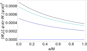
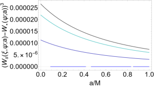
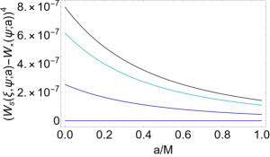
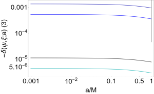
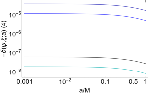
Figure 25: Difference $(W_{s}-W_{\times})^{\nu}$ (upper panels), defining the $\Gamma$–quantities introduced in Sec. (7), and the $\delta$-quantities (below panels) $-\delta(\nu)$ are shown as functions of the BH spin-mass ratio $a/M$, at different fluid momenta $\ell$ regulated by the $\psi$ parameters signed on the curves and different $K_{s}\equiv e^{W_{s}}$ parameters regulated by $\xi$, and different ${\nu}$–see Eq. (84). The $\Gamma$–quantities regulate the mass–flux, the enthalpy–flux (related to the temperature parameter), and the flux thickness. $\delta$–quantities regulate the cusp luminosity, the disk accretion rate, and the mass flow rate through the cusp i.e., mass loss accretion rat–see also Figs (19). $\Gamma$–quantities, have general form $\Gamma(r_{\times},r_{s},n)=\beta_{1}(n,\kappa)(W_{s}-W_{\times})^{\beta_{2}(n)}$, where here $\beta_{1}(n,\kappa)=1$ and $\beta_{2}(n))\equiv\nu$ are functions of the polytropic index and constant. $\delta$-quantities, while $\delta={\Gamma}(r_{\times},r_{s},n)r_{\times}/\Omega(r_{\times})$; where $\Omega(r_{\times})$ is the relativistic angular frequency at the tori cusp $r_{\times}$. Blue curves correspond to $(\psi=3;\xi=2)$; dark-blue curves to $(\psi=10;\xi=2)$, dark-cyan curves to $(\psi=3;\xi=10)$; and black curves to $(\psi=10;\xi=10)$.

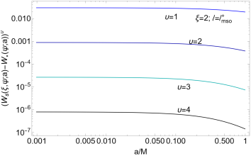
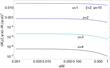
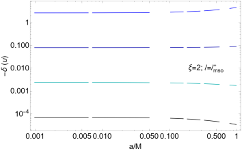
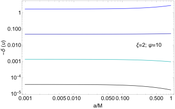
Figure 26: Upper panels show difference $(W_{s}-W_{\times})^{\nu}$ defining the $\Gamma$–quantities, and below panels show $\delta$-quantities, as functions of the BH spin-mass ratio $a/M$, at different fluid momenta $\ell$ regulated by the $\psi$ parameters and different $K_{s}\equiv e^{W_{s}}$ parameters regulated by $\xi$, and different ${\nu}$, signed on the curves–see Eq. (84) and Sec. (7). Panels show the situations for different $(\xi,\psi)$ or $(\xi,\ell)$, where blue curves correspond to $\nu=1$; dark-blue curves to $\nu=2$, dark-cyan curves to $\nu=3$; and black curves to $\nu=4$. The $\Gamma$–quantities regulate the mass–flux, the enthalpy–flux (related to the temperature parameter), and the flux thickness. $\delta$–quantities regulate the cusp luminosity, the disk accretion rate, and the mass flow rate through the cusp i.e., mass loss accretion rate. $\Gamma$–quantities, have general form $\Gamma(r_{\times},r_{s},n)=\beta_{1}(n,\kappa)(W_{s}-W_{\times})^{\beta_{2}(n)}$, where here $\beta_{1}(n,\kappa)=1$ and $\beta_{2}(n))\equiv\nu$ are functions of the polytropic index and constant. $\delta$-quantities, have general form $\delta={\Gamma}(r_{\times},r_{s},n)r_{\times}/\Omega(r_{\times})$; where $\Omega(r_{\times})$ is the relativistic angular frequency at the tori cusp $r_{\times}$ where the pressure vanishes.

Data availability

There are no new data associated with this article. No new data were generated or analysed in support of this research.

References

- Abramowicz (1971) Abramowicz M. A. 1971 Acta. Astron., 21, 81
- Abramowicz (1985) Abramowicz M. A. 1985 Astronomical Society of Japan, 37, 4, 727-734
- Abramowicz&Fragile (2013) Abramowicz M. A.&Fragile P.C. 2013 Living Rev. Relativity, 16, 1
- Alig et al. (2013) Alig C., Schartmann M., Burkert A. , Dolag K. 2013, APJ, 771, 2, 119
- Aly et al. (2015) Aly H., Dehnen W., Nixon C.& King A. 2015, Mon. Not. Roy. Astron. Soc., 449, 1, 65
- Amaro-Seoane et al. (2016) Amaro-Seoane, P., Maureira-Fredes, C., Dotti, M., et al. 2016, A&A, 591, A114.
- Balek et al. (1989) Balek V., Bicak J., Stuchlik Z., 1989, BAICz, 40, 133
- Blaschke&Stuchlík (2016) Blaschke M., Stuchlík Z., 2016, PhRvD, 94, 086006
- Bardeen (1972) Bardeen J. M., 1972, Rapidly Rotating Stars, Disks, and Black Holes in Black Holes Les Astres Occlus Les Houches, 1972 edited by C. DeWitt and B. S. DeWitt.
- Bardeen&Petterson (1975) Bardeen J. M., Petterson J. A., 1975, APJ, 195, L65
- Barrabes et al. (1995) Barrabes C., Boisseau B. and Israel W. 1995, MNRAS, 276, 432
- Beckert&Falcke (2002) Beckert T.&Falcke H., 2002, Astron. Astrophys. 388, 1106
- Bicak&Stuchlik (1976) Bicak J.& Stuchlik Z., 1976, BAICz, 27, 129
- Bonnerot et al. (2016) Bonnerot C., Rossi E.M., Lodato G. et al. 2016, MNRAS, 455, 2, 2253
- Carmona-Loaiza et al. (2015) Carmona-Loaiza J.M., Colpi M., Dotti M. et al., 2015,MNRAS,453,1608
- Carter (1968) Carter B., 1968, Phys. Rev., 174, 1559
- Chakrabarti (1990) Chakrabarti, S. K., 1990, MNRAS , 245, 747
- Chakrabarti (1991) Chakrabarti S. K., 1991, MNRAS, 250, 7
- Christodoulou et al. (2017) Christodoulou D. M., Laycock S. G. T., Kazanas D., 2017, MNRAS: Letters, 470, 1, L21–L24
- Christodoulou&Ruffini (1971) Christodoulou D. M.& Ruffini R., 1971, Phys. Rev. D,4, 3552
- Cowperthwaite&Reynolds. (2012) Cowperthwaite P. S.&Christopher S. R., 2012, ApJL, 752, L21
- Doğan et al. (2015) Doğan S., Nixon C., King A. et al., 2015, MNRAS, 449, 1251
- Dyda et al. (2015) Dyda S., Lovelace R. V. E, et al., 2015, MNRAS, 446, 613–621
- Ensslin (2003) Ensslin T. A., 2003, Astron. Astrophys. 401, 499-504
- Evans et al. (2010) Evans, D. A., Reeves, J. N., Hardcastle, M. J., et al. 2010, APJ, 710, 859.
- Event Horizon Telescope Collaboration et al. (2019) Event Horizon Telescope Collaboration, Akiyama K., Alberdi A., Alef W., Asada K., Azulay R., Baczko A.-K., et al., 2019, ApJL, 875
- Garofalo (2013) Garofalo D. 2013.,Advances in Astronomy, 2013, 213105
- Garofalo et al. (2010) Garofalo D., Evans D.A., Sambruna R. M. 2010, MNRAS, 406, 975-986
- Impellizzeri et al. (2019) Impellizzeri C. M. V. et al., 2019, ApJL, 884, L28
- Kataoka et al. (2007) Kataoka J. et al., 2007, PASJ, 59, 279
- King&Nixon (2018) King A.&Nixon C., 2018, APJ, 857, 1, L7
- King et al. (2005) King A. R., Lubow S. H., Ogilvie G. I.,& Pringle J. E. 2005 MNRAS, 363, 49
- Kozłowski et al. (1979) Kozłowski M., Jaroszyński M., Abramowicz M. A., 1998, Astron. Astrophys., 63, 209
- Kuznetsov et al. (1999) Kuznetsov O. A., et al., 1999, ApJ, 514, 691
- Kim et al. (2016) Kim M. I., Christian D. J., Garofalo D.& D’Avanzo J., 2016, MNRAS 460, 3, 3221–3231
- Lodato&Pringle (2006) Lodato G.& Pringle J. E. 2006, MNRAS, 368, 1196
- Lovelace&Chou (1996) Lovelace R. V. E.&Chou T. 1996, APJ, 468, L25
- Lovelace et al. (2014) Lovelace R.V.E., Romanova M.M. , Lii P. et al. 2015, Comp. Astroph. Cosmology, 1-3
- Martin et al. (2014) Martin R. G., Nixon C., Lubow S. H., et al. 2014, Astrophys. J. 792, L33
- Middleton et al. (2014) Middleton M. J.,Miller-Jones J. C. A., Fender R. P. 2014, MNRAS, 439, 2, 1740–1748
- Morningstar et al. (2014) Morningstar W. R., Miller J. M., Reis R. C. et al. 2014,APJ, 784, L18
- Murray et al. (1999) Murray J. R., de Kool M., Li J., 1999, ApJ, 515, 738
- Narayan et al. (2022) Narayan R., Chael A., Chatterjee K., Ricarte A., Curd B., 2022, MNRAS, 511
- Nealon et al. (2015) Nealon R., Price D. and Nixon C. 2015, MNRAS, 448, 2, 1526
- Nixon et al. (2011) Nixon C. J., Cossins P. J. , King A. R., Pringle J. E. 2011, MNRAS, 412, 3, 1591–1598
- Nixon et al. (2012a) Nixon, C. J., King, A. R.,&Price, D. J. 2012a, MNRAS, 422, 2547.
- Nixon et al. (2012b) Nixon C. J., King A. R.,& Price D. J., et al.2012b, Astrophys. J., 757, L24
- Nixon et al. (2013) Nixon C., King A.&Price D. 2013, MNRAS, 434, 1946
- Paczyński (1980) Paczyński B, 1980, Acta Astron., 30, 4
- Porth et al. (2021) Porth O., Mizuno Y., Younsi Z., Fromm C. M., 2021, MNRAS, 502, 2023
- Pugliese&Montani (2015) Pugliese D.& Montani G. 2015, Phys. Rev. D, 91, 8, 083011
- Pugliese&Montani (2018) Pugliese D.& Montani G. 2018, MNRAS, 476, 4, 4346-4361
- Pugliese&Montani (2021) Pugliese D.& Montani G. 2021, Gen. Rel. Grav., 53, 5,51
- Pugliese&Quevedo (2015) Pugliese D.&Quevedo H. 2015, Eur. Phys. J. C, 75, 5, 234
- Pugliese&Quevedo (2018) Pugliese D.&Quevedo H. 2018, Eur. Phys. J. C, 78, 1, 69
- Pugliese et al. (2011) Pugliese D., Quevedo H. and Ruffini R. 2011, Phys. Rev. D, 84, 044030
- Pugliese&Stuchlík (2015) Pugliese D.&Stuchlík Z. 2015, Astrophys. J.s, 221, 2, 25
- Pugliese&Stuchlík (2016) Pugliese D.&Stuchlík Z. 2016, Astrophys. J.s, 223, 2, 27
- Pugliese&Stuchlík (2017a) Pugliese D.&Stuchlík Z. 2017a, Astrophys. J.s, 229, 2, 40
- Pugliese&Stuchlik (2017b) Pugliese D.&Stuchlík Z. 2017b, Eur. Phys. J. C, 79, 4, 288
- Pugliese&Stuchlik (2018a) Pugliese D.&Stuchlík Z. 2018a,Class. Quant. Grav. 35, 18, 185008
- Pugliese&Stuchlik (2018b) Pugliese D.&Stuchlík Z 2018b, JHEAp, 17, 1
- Pugliese&Stuchlik (2018c) Pugliese D.&Stuchlík Z. 2018c Class. Quant. Grav., 35, 10, 105005
- Pugliese&Stuchlik (2020a) Pugliese D.& Stuchlik Z. 2020a, MNRAS., 493, 3, 4229–4255
- Pugliese&Stuchlik (2020b) Pugliese D.& Stuchlik Z., 2020b, Class.Quant.Grav., 37, 19, 195025
- Pugliese&Stuchlik (2021a) Pugliese D.&Stuchlík Z. 2021a, Class. Quant. Grav., 38, 14, 145014
- Pugliese&Stuchlik (2021b) Pugliese D.&Stuchlík Z. 2021b PASJ, 73, 5, 1333-1366
- Pugliese&Stuchlik (2021c) Pugliese D.&Stuchlík Z. 2021c PASJ,73 6, 1497-1539
- Pugliese&Stuchlík (2022) Pugliese D.&Stuchlík Z. 2022, in preparation
- Rao&Vadawale (2012) Rao A.&Vadawale S.V., 2012, ApJL, 757, L12
- Reis et al. (2013) Reis R. C. et al., 2013, ApJ, 778, 155
- Sadowski et al. (2016) Sadowski, A., Lasota, J.P., Abramowicz, M.A.&Narayan, R. 2016, MNRAS, 456, 4, 391
- Scheuerl&Feiler (1996) Scheuerl P. A. O.& Feiler R. 1996, MNRAS, 282, 291-294
- Stuchlik (1980) Stuchlik Z., 1980, BAICz, 31, 129
- Stuchlík (2005) Stuchlík Z., 2005, MPLA, 20, 561
- Stuchlík&Kološ (2016) Stuchlík Z., Kološ M., 2016, EPJC, 76, 32
- Stuchlík et al. (2020) Stuchlík Z., Kološ M., Kovář J., Slaný P., Tursunov A., 2020, Univ, 6, 26
- Stuchlík, Kološ,&Tursunov (2021) Stuchlík Z., Kološ M., Tursunov A., 2021, Univ, 7, 416
- Stuchlík&Schee (2012) Stuchlík Z., Schee J., 2012, CQGra, 29, 065002
- Stuchlík&Schee (2013) Stuchlík Z., Schee J., 2013, CQGra 30, 075012
- Stuchlík, Hledík,&Truparová (2011) Stuchlík Z., Hledík S., Truparová K., 2011, CQGra, 28, 155017
- Stuchlík, Slaný,&Kovář (2009) Stuchlík Z., Slaný P., Kovář J., 2009, CQGra, 26, 215013
- Tejeda et al. (2017) Tejeda E., Gafton E., Rosswog S., Miller J. C., 2017, MNRAS, 469, 4483
- Volonteri (2010) Volonteri, M. 2010, Accretion and Ejection in AGN: a Global View, 427, 3
- Volonteri et al. (2003) Volonteri M., Haardt F.,& Madau P., 2003 APJ, 582 559
- Wong et al. (2021) Wong G. N. et al., 2021, The Astrophysical Journal, 914:55
- Zanotti&Pugliese (2014) Zanotti O.&Pugliese D. 2015, Gen. Rel. Grav., 47, 4, 44
- Zhang et al. (1997) Zhang S. N., Cui W., Chen W., 1997, ApJ, 482, L155
- Zhang et al. (2015) Zhang W. et al., 2015,The Astrophysical Journal, 807:89