Filtering methods for coupled inverse problems

Abstract

We are interested in ensemble methods to solve multi-objective optimization problems. An ensemble Kalman method is proposed to solve a formulation of the nonlinear problem using a weighted function approach. An analysis of the mean field limit of the ensemble method yields an explicit update formula for the weights. Numerical examples show the improved performance of the proposed method.

1 Introduction

In many applications, it is often required to determine the model parameters that approximate observable and noisy data. In this work we are concerned with those inverse problems in a finite dimensional setting, i.e.,

$$y=\mathcal{G}(u)+\eta$$ (1)

where $\mathcal{G}$ is the (possible nonlinear) forward operator between the finite dimensional spaces $X=\mathbb{R}^{d}$ and $Y=\mathbb{R}^{k}$ with $d,k\in\mathbb{N}$, $u\in X$ is the unknown parameter, $y\in Y$ is the observation and $\eta\sim\mathcal{N}(0,\Gamma)$ is the observational noise where $\Gamma$ is a known covariance matrix. Given the noisy measurements, the observation and the mathematical model $\mathcal{G}$, we are interested in finding the corresponding control $u$. Certainly, those problems have been widely studied and different approaches have been proposed in the literature in order to overcome possible ill–posedness of the problem, see e.g. [12] for a survey.

In this work, we will focus on a particular numerical method for solving (1), namely the Ensemble Kalman Filter (EnKF). This method was introduced in the last decade [13], but has gained recent attention due to novel developments and insights, see e.g. [15, 16, 24] and references therein. The EnKF aims to solve a least–square formulation of the inverse problem and produces $u^{*}$ such that

$$u^{*}=argmin_{u\in X}\frac{1}{2}\left\lVert\Gamma^{-\frac{1}{2}}(y-\mathcal{G}(u))\right\rVert^{2}.$$ (2)

The EnKF is an iterative filtering method which sequentially updates each member of an ensemble $k=1,\dots,K$ of elements $u_{k}$ in the space $X$ by means of the Kalman update formula, using the knowledge of the model $\mathcal{G}$ and given observational data $y$. The method is gradient free and even for small number of ensembles $K$ satisfactory results have been reported [20]. Several contributions have been made regarding the application and analysis of this method, see e.g. [1, 2, 3, 8, 17, 18, 24, 25] and extensions to the constraint case [7].

Here, we are interested in a possible extension of the method towards a multi–objective minimization formulation. Those are also known as coupled inverse problems where for given data, a choice of parameters for competing models has to be determined. Examples of such problems stem from applications in geophysics [19] to oil and water reservoir problems [26]. We propose a formulation for general multi-objective optimization problems in the forthcoming section using a classical weighted function approach. By extending prior work [15] we will focus on suitable update strategies for the weights based on a mean field description of the method. Numerical results will be performed to highlight the properties of the proposed method.

2 On the Ensemble Kalman Filter (EnKF) for Coupled Inverse Problems

We consider $l$ coupled inverse problems for a set of parameters $u\in X$ and consider the simultaneous minimization of $\mathcal{G}_{1},\dots,\mathcal{G}_{l}$ models, given observations $y_{1},\dots,y_{l}\in Y$:

$$\min_{u\in X}\left(\|\Gamma^{-\frac{1}{2}}\left(y_{1}-\mathcal{G}_{1}(u)\right)\|,\dots,\|\Gamma^{-\frac{1}{2}}\left(y_{l}-\mathcal{G}_{l}(u)\right)\|\right).$$ (3)

The observational noise on the data $y_{i}$ is $\eta_{i}\sim\mathcal{N}(0,\Gamma)$ with fixed covariance matrix $\Gamma$. Finding $u$ that simultaneously solves (3) is called multi–objective or multi criteria optimization, see e.g. [11, 21, 22]. In the following we use the concept of Pareto optimality [22] that defines a notion of minimum for the vector–valued optimization problem (3):

Definition 2.1.

A point $u^{*}\in\mathbb{R}^{d}$ is called Pareto optimal if and only if there exists no point $u\in\mathbb{R}^{d}$ such that $\mathcal{G}_{i}(u)\leq\mathcal{G}_{i}(u^{*})$ for all $i=1,2,\dots,l$ and $\mathcal{G}_{j}(u)\leq\mathcal{G}_{j}(u^{*})$ for at least one $j\in\{1,2,\dots,l\}$.

The set $\mathcal{S}_{U}$ of all $u^{*}$ fulfilling Definition (2.1) is called Pareto set, while its representation in the space of objectives $\mathcal{S}_{G}:=\{\left(y_{i}-\mathcal{G}_{i}(u)\right)_{i=1}^{l}:u\in\mathcal{S}\}$ is called Pareto front. An approach based on a weighted function approach [21] is followed to compute $\mathcal{S}_{G}:$ Given a vector $\mathbf{\mathbb{\lambda}}\in\Lambda$ where

$$\Lambda:=\{\mathbf{\mathbb{\lambda}}\in\mathbb{R}^{l}_{+}:\mathbf{\mathbb{\lambda}}\cdot\mathbf{1}=1\}$$ (4)

and $\mathbf{1}=(1,\dots,1)^{T},$ we define the weighted objective function

$$\mathcal{G}(u,\mathbf{\mathbb{\lambda}}):=\sum\limits_{i=1}^{\ell}\mathbf{\mathbb{\lambda}}_{i}\mathcal{G}_{i}(u):X\times\Lambda\to Y.$$ (5)

The convex combination of the observations is given by $y=\sum\limits_{i=1}^{\ell}\mathbf{\mathbb{\lambda}}_{i}y_{i}.$ An approximation to the Pareto front $\mathcal{S}_{U}$ is then obtained by

$${P}:=\{u^{*}(\mathbb{\lambda}):\mathbb{\lambda}\in\Lambda\},$$ (6)

where

$$u^{*}(\mathbb{\lambda})=argmin_{u\in X}\Phi(u,\mathbb{\lambda}),\;\Phi(u,y,\mathbb{\lambda})=\frac{1}{2}\left\lVert\Gamma^{-\frac{1}{2}}\sum_{i=1}^{l}\mathbb{\lambda}_{i}\left(y_{i}-\mathcal{G}_{i}(u)\right)\right\rVert^{2}.$$ (7)

In case of a convex problem, $S_{U}=P$, see [21, Theorem 3.1.4]. Note that $\Lambda$ is also called the probability simplex [4].

2.1 EnKF and Mean Field Description of Parameterized Problem (7)

For the efficient computation of the Pareto front (6) we propose an ensemble based method following recent work [15, 16, 24]. For a fixed value of $\mathbb{\lambda}\in\Lambda$, the EnKF method samples $J>0$ initial values $u^{j,0}\in X$ and iterate according to equation (9) for some $\Delta t>0.$ Under suitable assumptions on $\mathcal{G}$ it has been shown in [24], that

$$\lim\limits_{J\to\infty}\frac{1}{J}\sum\limits_{j=1}^{J}u^{j,n}(\mathbb{\lambda})=u^{\ast}(\mathbb{\lambda}),$$ (8)

where $u^{\ast}(\mathbb{\lambda})$ solves equation (7), [10, Theorem 1]. For further results on stability we refer to [15, 24]. For $y$ and $\mathcal{G}$ defined by (5) each member $j$ of the ensemble is propagated according to

$$u^{j,n+1}=u^{j,n}+C(U^{n})\left(D(U^{n})+\frac{1}{\Delta t}\Gamma^{-1}\right)^{-1}\left[y-\mathcal{G}(u^{n},\lambda)\right],$$ (9)

where $C(U^{n})$ and $D(U^{n})$ are the covariance matrices depending on the set of ensembles $U^{n}(\mathbb{\lambda})$ at the iteration $n$ and on $\mathcal{G}(U^{n})$:

$$U^{n}(\mathbb{\lambda}) =\{u^{j,n}(\mathbb{\lambda})\}_{j=1}^{J},$$ (10)

$$\bar{U}^{n} :=\frac{1}{J}\sum_{k=1}^{J}u^{j,n}(\mathbb{\lambda}),\;\bar{\mathcal{G}}:=\frac{1}{J}\sum_{k=1}^{J}\sum_{i=1}^{l}\mathbb{\lambda}_{i}\mathcal{G}_{i}(u^{j,n}(\mathbb{\lambda}),\mathbb{\lambda})),$$ (11)

$$C(U^{n}(\mathbb{\lambda}))= \frac{1}{J}\sum_{k=1}^{J}(u^{k,n}(\mathbb{\lambda})-\bar{U}^{n})\otimes(\mathcal{G}(u^{k,n}(\mathbb{\lambda}),\mathbb{\lambda})-\bar{\mathcal{G}}),$$ (12)

$$D(U^{n}(\mathbb{\lambda}))= \frac{1}{J}\sum_{k=1}^{J}\left[\mathcal{G}(u^{n}(\mathbb{\lambda}),\mathbb{\lambda}))-\bar{\mathcal{G}}\right]\otimes\left[\mathcal{G}(u^{n}(\mathbb{\lambda}),\mathbb{\lambda})-\bar{\mathcal{G}}\right].$$ (13)

Several extensions have been studied and we refer to the references above for more details. Also, the limiting equation for $\Delta t\to 0$ under the scaling $\Gamma^{-1}=\Delta t\Gamma^{-1}$ of the previous dynamics has been studied and analyzed, e.g. [24, 15]. In the case $\Delta t\to 0$ and $J\to\infty$ a mean field limit is obtained. Rigorous results can be found e.g. in [15] and in [23, 6] for general mean field results on interacting particle systems. Since there is no dynamics in $\lambda$ the following result is a simple consequence of the existing results for the convergence for $J\to\infty$ given e.g. in [5, 10, 14, 15, 16, 24], in particular [24, Theorem 3].

Proposition 2.2.

Assume $\mathcal{G}_{i}(u)=G_{i}u$ for $i=1,\dots,l$ and let $\Phi$ be given by equation (7). Let $\mathcal{P}(X)$ be the space of probability measures on $X$ equipped with the 1-Wasserstein distance.

Let $J>0$ and assume $u^{j,0}\in X$ for $j=1,\dots,J$ given and denote by $f^{U}_{0}(v)=\frac{1}{J}\sum_{j=1}^{J}\delta\left(u^{j,0}-v\right)$ the empirical measure associated to the initial data. The empirical measure

$$f^{U}(v,\mathbb{\lambda},t)=\frac{1}{J}\sum_{j=1}^{J}\delta\left(u^{j}(t,\mathbb{\lambda})-v\right)\in\mathcal{P}(X\times\Lambda\times\mathbb{R}^{+})$$ (14)

where $u^{j}(t,\mathbb{\lambda})$ fulfills for all $j=1,\dots,J$

$$\frac{d}{dt}u^{j}(t,\mathbb{\lambda}) =-C(U(t,\mathbb{\lambda}))\nabla\Phi(u^{j}(t,\mathbb{\lambda}),y,\mathbb{\lambda}),\;u^{j}(t,\mathbb{\lambda})=u^{j,0},$$ (15)

$$\mathcal{C}(U) =\frac{1}{J}\sum_{j=1}^{J}(u^{j}-\bar{U})\otimes(u^{j}-\bar{U}),\;\bar{U}=\frac{1}{J}\sum\limits_{j=1}^{J}u^{j},$$ (16)

is a solution in the distributional sense to the mean field equation

$$\partial_{t}f(v,\mathbb{\lambda},t)-\nabla_{v}\cdot\left(\mathcal{C}(t,\mathbb{\lambda})\nabla_{v}\Phi(u,y,\mathbb{\lambda})f(v,\mathbb{\lambda},t)\right)=0,\;f(v,\lambda,0)=f_{0}(v),$$ (17)

subject to initial data $f_{0}(v,\mathbb{\lambda})\in\mathcal{P}(X,\Lambda)$ and where the nonlocal operator $C(t,\mathbb{\lambda})=C[f](t,\mathbb{\lambda})$ is given by

$$(\mathcal{C}[f](\mathbb{\lambda},t))_{k,i}=\int_{X}v_{k}v_{i}f(v,\mathbb{\lambda},t)\,dv-\int_{X}v_{k}f(v,\mathbb{\lambda},t)\,dv\int_{X}v_{i}f(v,\mathbb{\lambda},t)\,dv,\;(k,i)=1,\dots,d.$$ (18)

Furthermore, if for $J\to\infty$ we have $W_{1}(f^{U}_{0},f_{0})\to 0$ for some $f_{0}\in\mathcal{P}(X),$ then for any $t\geq 0$ we have $W_{1}(f^{U}(\cdot,t),f(\cdot,t))\to 0,$ where $f$ is a solution in the distributional sense to (17).

Denote by $P(t)$ an approximation to $P$ expressed in terms of the probability density $f(\cdot,t)$ by

$${P}(t)=\left\{\int_{X}u\;df(u,\mathbb{\lambda},t):\;\mathbb{\lambda}\in\Lambda\right\}.$$ (19)

Due to the convergence of the particles to $u^{\ast}(\lambda)$, we expect that for $t\to\infty,$ the set $P(t)$ approaches the set $P$ given by (6), see [16] for the corresponding result in the case independent of $\lambda.$

The mean field equation is independent of the ensemble size $J$ and therefore possibly attractive for numerical methods. For an efficient computation of $P(t)$ the solution to equation (17) for any $\lambda\in\Lambda$ is required. In numerical discretization of equation (17) a suitable grid in $\lambda$ is hence necessary. In the following aim to provide a method to develop a strategy for choosing those quadrature points in $\Lambda.$ This is obtained by considering the sensitivity of $f$ with respect to $\lambda.$

2.2 Sensitivity of Mean Field and Moment Equations

The sensitivity of $f$ with respect to $\lambda$ can be studied e.g. by formally differentiating the meanfield equation (17) leading to the set of equations $i=1,\dots,l$

$$0 =\partial_{t}\partial_{\lambda_{i}}f(v,\lambda,t)-\nabla_{v}\partial_{\lambda_{i}}\Big{(}C\ \nabla_{v}\Phi(v,y,\lambda)f(v,\lambda,t)\Big{)}$$ (20)

$$=\partial_{t}\partial_{\lambda_{i}}f(v,\lambda,t)-\nabla_{v}\Big{(}\partial_{\lambda_{i}}C\nabla_{v}\Phi(v,y,\lambda)f(v,\lambda,t)+$$ (21)

$$\qquad C\ \partial_{\lambda_{i}}(\nabla_{v}\Phi(v,y,\lambda))f(v,\lambda,t)+C\ \nabla_{v}\Phi(v,y,\lambda)\partial_{\lambda_{i}}f(v,\lambda,t)\Big{)}$$ (22)

$$=:\partial_{t}\partial_{\lambda_{i}}f(v,\lambda,t)-\nabla_{v}\Big{(}T_{1}+CT_{2}f(v,\lambda,t)+C\ \nabla_{v}\Phi(v,y,\lambda)\partial_{\lambda_{i}}f(v,\lambda,t)\Big{)}.$$ (23)

where $C=C[f](\lambda,t)$ is given by equation (18). Since the initial data in (17) is assumed to be independent of $\mathbb{\lambda}$ we obtain for $i=1,\dots,l$

$$\partial_{\lambda_{i}}f(v,\lambda,0)=0.$$ (24)

Under the assumption of Proposition 2.2, namely,

$$\mathcal{G}_{i}(u)=G_{i}u,\;i=1,\dots,l,$$ (25)

some terms of equation (20) can be further simplified to

$$T_{1}:= \partial_{\lambda_{i}}C\ \nabla_{v}\Phi(v,y,\lambda)f=(E_{\lambda_{i}}-2m_{\lambda_{i}}\otimes m)\ \nabla_{v}\Phi(v,y,\lambda)f,$$ (26)

$$T_{2}:= \frac{\partial(\nabla_{v}\Phi)}{\partial\lambda_{i}}=\partial_{\lambda_{i}}\Big{(}(\mathcal{G})^{T}\Gamma^{-1}(y-\mathcal{G}v)\Big{)}$$ (27)

$$=(\sum_{i=1}^{l}\mathcal{G}_{i})^{T}\Gamma^{-1}\Big{(}y-\mathcal{G}v\Big{)}+\left(\mathcal{G}\right)^{T}\Gamma^{-1}\Big{(}\sum_{i=1}^{l}y_{i}-\mathcal{G}_{i}v\Big{)}.$$ (28)

Computationally solving system (2.1) to obtain sensitivity information on $\lambda$ is prohibitive. However, $P(t)$ given by equation (19) only depends on the first moment of $f$ and not on the full solution. Hence, we consider only sensitivity of the moments of the solution, i.e., define the first and second moments of $f$ as

$$m(\mathbb{\lambda},t)=\int_{X}vdf(v,\mathbb{\lambda},t)\in\mathbb{R}^{d},\;E(\mathbb{\lambda},t)=\int_{X}v\otimes vdf(v,\mathbb{\lambda},t)\in\mathbb{R}^{d\times d}.$$ (29)

Then, for $i=1,\dots,l$, the sensitivity of $(m,E)$ is given by

$$\frac{\partial m}{\partial\lambda_{i}}=\int vd\frac{\partial f}{\partial\lambda_{i}}(v,\lambda,t),\;\frac{\partial E}{\partial\lambda_{i}}=\int v\otimes vd\frac{\partial f}{\partial\lambda_{i}}(v,\lambda,t)$$ (30)

and they fulfill a closed coupled system of equations of ordinary differential equations obtained by integration of equation (20) given by the system (31).

Lemma 2.3.

Assume (25) and let $\Phi$ be given by equation (7). If $f=f(v,\mathbb{\lambda},t)\in\mathcal{P}(X\times\Lambda\times\mathbb{R}^{+})$ with finite second moment and $\nabla_{\lambda}f$ be differentiable solution to (17) with initial data $f(v,\lambda,0)=f_{0}(v)\in\mathcal{P}(X)$ and to equation (20) with initial data (24).

Then, the moments $(m,E)$ and their derivatives fulfill the following system of ordinary differential equations for $i=1,\dots,l$

$$\begin{cases}\frac{d}{dt}m&=-CG^{T}\Gamma^{-1}\left(y-G\ m\right)\\ \frac{d}{dt}m_{\lambda_{i}}&=-(\partial_{\lambda_{i}}C)G^{T}\Gamma^{-1}(y-G\ m)-C(\partial_{\lambda_{i}}G)^{T}\Gamma^{-1}(y-Gm)\\ &-CG^{T}\Gamma^{-1}\left(\partial_{\lambda_{i}}y-(\partial_{\lambda_{i}}G)m\right)+CG^{T}\Gamma^{-1}Gm_{\lambda_{i}}\\ \frac{d}{dt}E&=-CG^{T}\Gamma^{-1}(y\otimes m-GE)-[CG^{T}\Gamma^{-1}(y\otimes m-GE)]^{T}\\ \frac{d}{dt}E_{\lambda_{i}}&=-CG^{T}\Gamma^{-1}\left(y\otimes m_{\lambda_{i}}-GE_{\lambda_{i}}\right)-\bar{C}_{i}G^{T}\Gamma^{-1}\left(y\otimes m-GE\right)\\ &-C\partial_{\lambda_{i}}G^{T}\Gamma^{-1}(y\otimes m-GE)-CG^{T}\Gamma^{-1}(\partial_{\lambda_{i}}ym-\partial_{\lambda_{i}}GE)\\ &-[CG^{T}\Gamma^{-1}\left(y\otimes m_{\lambda_{i}}-GE_{\lambda_{i}}\right)]^{T}-[\bar{C}_{i}G^{T}\Gamma^{-1}\left(y\otimes m-GE\right)]^{T}\\ &-[C\partial_{\lambda_{i}}G^{T}\Gamma^{-1}(y\otimes m-GE)]^{T}-[CG^{T}\Gamma^{-1}(\partial_{\lambda_{i}}ym-\partial_{\lambda_{i}}GE)]^{T}\\ C&=E-m\otimes m,\\ {\bar{C}}_{i}&=E_{\lambda_{i}}-2m_{\lambda_{i}}\otimes m.\end{cases}$$ (31)

and initial data independent of $\lambda$

$$m(0)=\int_{X}vdf_{0}(v),\;E(0)=\int_{X}v\otimes vdf_{0}(v),\;m_{\lambda_{i}}(0)=0,\;E_{\lambda_{i}}(0)=0.$$ (32)

For any time $T>0,$ there exists a unique solution $(m,E,\partial_{\lambda_{1}}m,\partial_{\lambda_{1}}E,\dots,,\partial_{\lambda_{l}}m,\partial_{\lambda_{l}}E,)\in C^{1}(0,T;\mathbb{R}^{(l+1)\cdot(d+d\times d)})$ to the system (31).

Proof.

The right hand side of (31) is Lipschitz with respect to $(m,m_{\lambda_{i}},E,E_{\lambda_{i}})$ which yields the existence and uniqueness of the moments. The derivation of the moment system is given by integration based on the formal equation (20). For simplicity, we assume in the following proof that $f$ is absolutely continuous with respect to the Lebesgue measure. We denote the induced density also by $f.$

First, note that since $\partial_{\lambda_{i}}f$ is a conservative equation with initial data (24) and therefore

$$\int_{X}\partial_{\lambda_{i}}f(v,\lambda,t)dv=0.$$ (33)

Second, the first and the third equation of system (31) follow immediately by integration of the mean field equation (17). Indeed for the third equation we obtain

$$\partial_{t}\int_{X}v_{i}v_{j}f\ dv-\sum_{k=1}^{d}\int v_{i}v_{j}\partial_{k}(C\nabla_{v}\Phi(v,y,\lambda)f)_{k}\ dv=0,\quad i,j=1,\dots,d,$$ (34)

and, integrating by parts

$$\partial_{t}E_{i,j}+\sum_{k=1}^{d}\int\partial_{k}(v_{i}v_{j})(C\nabla_{v}\Phi(v,y,\lambda)f)_{k}\ dv=0.$$ (35)

Thus

$$\partial_{t}E_{i,j}+\int\left[(C\nabla_{v}\Phi(v,y,\lambda))_{i}v_{j}f+(C\nabla_{v}\Phi(v,y,\lambda))_{j}v_{i}f\right]dv=0,$$ (36)

$$\partial_{t}E_{i,j}+\sum_{l=1}^{d}(CG^{T}\Gamma^{-1})_{i,l}y_{l}m_{j}-\sum_{l=1}^{d}(CG^{T}\Gamma^{-1}G)_{i,l}E_{l,j}$$ (37)

$$+\sum_{l=1}^{d}(CG^{T}\Gamma^{-1})_{j,l}y_{l}m_{i}-\sum_{l=1}^{d}(CG^{T}\Gamma^{-1}G)_{j,l}E_{l,i}=0.$$ (38)

Hence, we obtain equation (31)

$$\partial_{t}E+CG^{T}\Gamma^{-1}(y\otimes m-GE)+\left[CG^{T}\Gamma^{-1}(y\otimes m-GE)\right]^{T}=0.$$ (39)

Since the operator $C$ is linear in $f$ we obtain

$$\frac{\partial C}{\partial\mathbb{\lambda}_{i}}=E_{\lambda_{i}}-2m_{\lambda_{i}}\otimes m,$$ (40)

and similar to term $T_{2}:$

$$\frac{\partial(\nabla_{v}\Phi)}{\partial\mathbb{\lambda}_{i}} =(\sum_{i=1}^{l}G_{i})^{T}\Gamma^{-1}\Big{(}y-Gv\Big{)}+\left(G\right)^{T}\Gamma^{-1}\Big{(}\sum_{i=1}^{l}y_{i}-G_{i}v\Big{)}.$$ (41)

Hence, integration of (20) yields

$$\partial_{t}m_{\lambda_{i}}+\Big{(}E_{\lambda_{i}}-2m_{\lambda_{i}}\otimes m\Big{)}\int_{X}\nabla_{v}\Phi(v,y,\mathbb{\lambda})f\ dv+$$ (42)

$$C\int_{X}\Big{(}(\sum_{i=1}^{l}G_{i})^{T}\Gamma^{-1}\Big{(}y-Gv\Big{)}+\left(G\right)^{T}\Gamma^{-1}\Big{(}\sum_{i=1}^{l}(y_{i}-G_{i}v)\Big{)}f\,dv$$ (43)

$$+C\int_{X}\nabla_{v}\Phi(v,y,\mathbb{\lambda})\partial_{\mathbb{\lambda}_{i}}f\ dv=0.$$ (44)

Due to assumption (25) the integrals involving $\nabla_{v}\Phi$ are computed explicitly

$$\int_{X}\nabla_{v}\Phi(v,y,\mathbb{\lambda})f\ dv =\int_{\mathbb{R}^{d}}G^{T}\Gamma^{-1}(y-Gv)f\ dv=G^{T}\Gamma^{-1}\left(y-G\ m\right),$$ (45)

$$\int_{X}\nabla_{v}\Phi(v,y,\mathbb{\lambda})\partial_{\mathbb{\lambda}_{i}}f\ dv =G^{T}\Gamma^{-1}\left(y\int_{\mathbb{R}^{d}}\partial_{\mathbb{\lambda}_{i}}fdv-G\int_{\mathbb{R}^{d}}v\partial_{\mathbb{\lambda}_{i}}fdv\right)=+G^{T}\Gamma^{-1}G\ m_{\lambda_{i}}.$$ (46)

Furthermore, we obtain

$$C \int_{X}\Big{(}(\sum_{i=1}^{l}G_{i})^{T}\Gamma^{-1}\Big{(}y-Gv\Big{)}+\left(G\right)^{T}\Gamma^{-1}\Big{(}\sum_{i=1}^{l}(y_{i}-G_{i}v)\Big{)}f\,dv$$ (47)

$$= C(\sum_{i=1}^{l}G_{i})^{T}\Gamma^{-1}(y-Gm)+C\left(G\right)^{T}\Gamma^{-1}\left(\sum_{i=1}^{l}(y_{i}-\mathcal{G}_{i}m)\right),$$ (48)

leading to the equation for $m_{\lambda_{i}}.$ The equations for $\frac{d}{dt}E_{\lambda_{i}}$ are obtained using a similar computation. ∎

Some remarks are in order.

• Note that the approximation to the Pareto front $P(t)$ on the mean field level is given by

  $$P(t)=\{m(\lambda,t):\lambda\in\Lambda\}.$$ (49)

  Hence, solving a coupled system of ordinary differential equations of dimension $(l+1)\times(d+d^{2})$ leads to information on $\nabla_{\lambda}m(t).$ This allows to obtain information for an adaptive strategy for the choice of $\lambda$ as follows: Assume for a fixed $\overline{\lambda},$ the optimal state is given by $m(\overline{\lambda},T)$ for some $T$ fixed and sufficiently large. Then, we may use a Taylor expansion of $m$ to obtain

  $$m(\overline{\lambda}+\Delta\lambda,T)=m(\overline{\lambda},T)+\Delta\lambda\cdot\nabla m(\overline{\lambda},T)+h.o.t.,$$ (50)

  where $\nabla m(\lambda,t)=\left(m_{\lambda_{i}}\right)_{i=1}^{l}$. The previous expansion can be used in two ways: For a given update $\Delta\lambda\in\mathbb{R}^{l}$ such that $\overline{\lambda}+\Delta\lambda\in\Lambda$, equation (50) yields an approximation on the new optimal value of the Pareto front $P(t)$. Second, we observe that the system (31) can be solved independently of the dynamics of $f=f(v,\lambda,t)$ leading to a family of solutions for $\lambda\in\Lambda$ and $t\geq 0$

  $$\left(m(\lambda,t),\;\nabla m(\lambda,t)\right),$$ (51)

  that can be computed a priori. We are interested in obtaining a discrete choice of $\lambda^{k}\in\Lambda$ for $k=1,\dots,K$ such that the Pareto set $S_{U}=\{ u^{*}(\lambda):\lambda\in\Lambda\}$ is approximated without clustering. Since for $T$ large we have $m(\lambda,T)\approx u^{*}(\lambda)$ we may utilize equation (50) to determine at least the norm of the update $\Delta\lambda=\lambda^{k+1}-\lambda^{k}$ such that the distance on $S_{U}$ is bounded by a given tolerance $\delta>0$ by requiring

  $$\|\Delta\lambda\|\|\nabla m(\lambda^{k})\|\leq\delta.$$ (52)

  This choice leads to numerical results shown later that also approximates the Pareto front $S_{G}$ very well with only a few discretization points $k=1,\dots,K$ in $\Lambda.$

• The convergence results on the EnKF require usually $n$ or $t$, respectively to tend to infinity. In the particular situation where the system of ordinary differential equations allows for steady–state solutions $(m,E,\nabla m,\nabla E)$, this value is therefore expected to be also a solution to the Pareto problem. The following equations characterize the steady–state solutions to (31) for $i=1,\dots,l$ only in the case d=1:

  $$Gm={y},\qquad m_{\mathbb{\lambda}_{i}}=c_{1,i},\qquad G^{2}E={y^{2}},\qquad E_{\mathbb{\lambda}_{i}}=c_{2,i},$$ (53)

  $$m=c_{1},\qquad m_{\mathbb{\lambda}_{i}}=c_{1,i},\qquad E=m^{2}, E_{\lambda_{i}}=2m\ m_{\mathbb{\lambda}_{i}}.$$ (54)

  where, $c_{1,i}$ and $c_{2,i}$ are arbitrary constants. Note that if $(m,E)$ is a set of moments of an underlying distribution function $f_{\infty}(u,\lambda),$ then by definition we obtain that $E\geq m^{2}$ imposing restrictions on the set of admissible constants $c_{k,i}$ for $k=1,2$ and $i=1,\dots,l,$.

• The case ${\bf d=1}$ also allows for an explicit computations of the Pareto front are possible, provided that the operator $\mathcal{G}=\sum\limits_{i=1}^{l}\lambda_{i}G_{i}u:X\to Y$ is invertible. In this case, the true solution is given by

  $$u^{*}(\mathbb{\lambda})=\mathcal{G}^{-1}y$$ (55)

  and on the mean field level, we expect $f(v,\lambda,t)=\delta(v-u^{*}(\mathbb{\lambda}))$ to be the stationary solution. In fact, the following computation verifies that $f$ is a stationary state of the moment system (31). Note that this particular probability measure $f$ defines a distribution on the set of functions $\psi\in C^{\infty}_{0}(X)$ by

  $$f[\psi]:=\int_{X}\psi(u)df(u,\lambda,t)=\psi(u^{*}(\mathbb{\lambda})).$$ (56)

  Hence, for $\psi(u)=u$ we obtain $Gm(\lambda,t)=y$ and for $\psi(u)=u^{2}$ we have $G^{2}E(\lambda,t)=y^{2}.$ Assuming that $\lambda\to u^{*}(\lambda)$ is differentiable with respect to $\lambda,$ the weak derivative is

  $$f_{\mathbb{\lambda}_{i}}[\psi]=\psi^{\prime}(u^{*}(\mathbb{\lambda}))u^{*}_{\lambda_{i}}(\mathbb{\lambda}),$$ (57)

  and hence, $m_{\lambda_{i}}=u^{*}_{\lambda_{i}}(\mathbb{\lambda})$ and $E_{\lambda_{i}}=2mm_{\lambda_{i}}^{2}$. Since $\mathcal{G}u^{*}(\lambda)=y$ we obtain that $\partial_{\lambda_{i}}\mathcal{G}\;u^{*}(\lambda)=-\mathcal{G}u_{\lambda_{i}}^{*}(\lambda)+\partial_{\lambda_{i}}y$ leading to the equality $\partial_{\lambda_{i}}\mathcal{G}\;m=-\mathcal{G}m_{\lambda_{i}}+\partial_{\lambda_{i}}y$. Hence, it is a steady state of equation (31).

3 Computational Results

For a numerical solution to the approximation of the Pareto front $S_{U}$ and $S_{G},$ respectively, we compare two strategies. In the direct approach we sample on an equidistant grid on $\Lambda$ the values of $\lambda^{k}$. In an adaptive strategy the solution to the mean field moment system (31) is utilized. Without loss of generality, in the numerical tests we assume $l=2$, so that $\mathcal{G}(u)=\mathbb{\lambda}\mathcal{G}_{1}(u)+(1-\mathbb{\lambda})\mathcal{G}_{2}(u)$ and such that $\Lambda$ is parameterized by a single parameter $\lambda\in[0,1].$ Moreover, we set $y=0$, $\eta=0$, $\Gamma=\mathbb{1}$ and $T_{fin}=10$ for all computations. To solve (31), we use a Matlab function ode45 and initial data recovered from the ensemble particles, i.e., $m_{0}=\frac{1}{J}\sum_{j=1}^{J}u_{j}$, $E_{0}=\frac{1}{J}\sum_{j=1}^{J}u_{j}^{2}$, $m_{\lambda_{i},0}=0$, $E_{\lambda_{i},0}=0$.

Even so the theory is presented in the linear case only, we present numerical results on nonlinear objective functions $\mathcal{G}_{i}$ in the numerical tests. Note that the existing literature on convergence and stability of the EnKF do not cover the nonlinear case, even in the case of only finitely many particles. Numerically, we propose two possible strategies to adapt method to the nonlinear case. In the first case and if the derivative of $\mathcal{G}$ is computable, we may linearize (7) up to the first order:

$$\left\lVert y-\mathcal{G}(u)\right\rVert\approx\left\lVert y-\mathcal{G}(u_{0})+\mathcal{G}^{\prime}(u_{0})u_{0}-\mathcal{G}^{\prime}(u_{0})u\right\rVert=\left\lVert\tilde{y}-\mathcal{G}^{\prime}(u_{0})u\right\rVert.$$ (58)

Replacing the nonlinear objective by its linearized version allows to apply the aforementioned results. However, an advantage of the EnKF is that it also applies to functions where no derivative information is available. Therefore, we secondly, consider $\mathcal{G}(m)$ instead of $G\;m$ in system (31). This simple heuristic modification is not justified by a moment analysis, since, in fact, the moment system in the nonlinear case is not closed.

3.1 Direct approach

Starting from an initial ensemble $u^{0}_{j}$ for $j=1,\dots,J$ and a set of fixed vectors $\mathbb{\lambda}_{k}\in\Lambda$ for $k=1,\dots,N_{\lambda}$, the particles are updated following (9). As in [9] we chose the vectors to be equispaced. The algorithm is described in detail in Figure 1.

Algorithm 1 Direct approach

1:Given $J$ samples $u_{j}^{0}$, with $j=1,\dots,J$ and a vector $\mathbb{\lambda}_{0_{i}}$, $i=0,\dots,l$

2:Set $n=0$, $t^{0}=0$ and final time $T_{fin}$ sufficiently large

3:for $k=1,2,\ldots,N_{\mathbb{\lambda}}$ do

4:     Solve the EnKF procedure: $\mathcal{G}=\mathbb{\lambda}_{k_{i}}\cdot\mathcal{G}_{i}$, $y=\mathbb{\lambda}_{k_{i}}\cdot y_{i}$

5:     while $t^{n}\leq T_{fin}$ do

$$u_{j}^{n+1} =u_{j}^{n}+C(\boldsymbol{u}^{n})\left(D(\boldsymbol{u}^{n})+\frac{1}{\Delta t}\Gamma^{-1}\right)^{-1}\left[y_{j}-\mathcal{G}({u}_{j}^{n})\right]$$

$$C(\boldsymbol{u}^{n}) =\frac{1}{J}\sum_{j=1}^{J}(u_{j}^{n}-\overline{\boldsymbol{u}}^{n})\otimes(\mathcal{G}(u_{j}^{n})-\overline{\mathcal{G}})$$ (EnKF)

$$D(\boldsymbol{u}^{n}) =\frac{1}{J}\sum_{j=1}^{J}\left[\mathcal{G}(u_{j}^{n})-\overline{\mathcal{G}}\right]\otimes\left[\mathcal{G}(u_{j}^{n})-\overline{\mathcal{G}}\right]$$

6:     end while

7:     The mean $\frac{1}{J}\sum\limits_{j=1}^{J}u^{T_{fin}}_{j}$ is an approximation to $u^{*}(\lambda)$

8:end for

3.2 Adaptive strategy

In the adaptive strategy the vector $\mathbb{\lambda}_{k}$ is obtained iteratively for $k=1,\dots$ according to equation (52). Intuitively, the equation yields a denser set of vectors $\lambda_{k}$ where the slope of the Pareto set $S_{U}$ measured through $\|\nabla m(\lambda_{k})\|$ is large. In order to state the update formula an ordering on $\Lambda$ is introduced as lexicographic order on the set $\Lambda$. The adaptive strategy using the update given by equation (52) is given below in Figure 2.

Algorithm 2 Adaptive approach

1:Given $J$ samples $u^{j,0}$, with $j=1,\dots,J$ and the update constant $\delta>0$

2:set $n=0$, $t^{0}=0$, the final time $T_{fin}$ and $\mathbb{\lambda}_{1}=0$

3:while $\mathbb{\lambda}_{k}<1$ do

4:     $\bar{u}_{k}\leftarrow$ solving the EnKF procedure (as in Step 5 of the Direct Approach)

5:     $[m,m_{\mathbb{\lambda}},E,E_{\mathbb{\lambda}}]\leftarrow$solve the ODE system (31) with initial conditions (32)

6:     $\bar{u}^{0}_{k+1}\leftarrow$ sampling from a Gaussian prob. distr. with mean $m$ and variance $E$

7:      $\mathbb{\lambda}_{k+1}\leftarrow\mathbb{\lambda}_{k}+\frac{\delta}{\left\lVert m_{\mathbb{\lambda}}\right\rVert}e_{lo}$, $e_{lo}$ the direction defined by the lexicographic order

8:end while

3.3 Test 1: Convex Example

As numerical test we consider the minimization of two convex functions $\mathcal{G}_{1},\mathcal{G}_{2}$:

$$\mathcal{G}_{1}=\left(u-\frac{1}{2}\right)^{2}\qquad\mathcal{G}_{2}=\left(u+\frac{1}{2}\right)^{2}.$$ (59)

The initial ensemble is chosen using the uniform distribution $U_{0}\sim\mathcal{U}(-1,1)$ and we use $J=20$. A comparison of the direct and the adaptive algorithm with $\delta=10^{-3}$ and $N_{\mathbb{\lambda}}=25$ is presented. The approximation of the Pareto front $S_{G}$ is shown in Fig. 1.

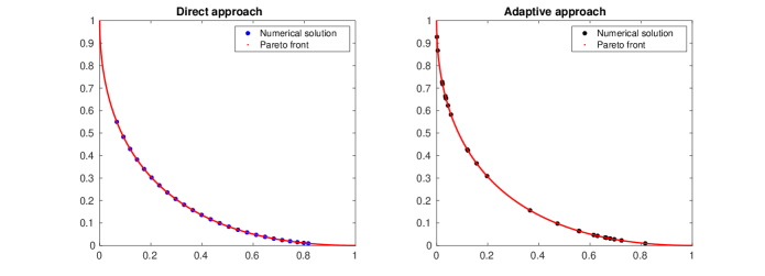
Figure 1: Test 1. Numerical approximation of the Pareto front, with the direct approach (left) and the adaptive approach (right). The red line is the analytical Pareto front. The dots indicate the mean of the ensemble at final time.

Different behavior of the two procedures is observed, where the solution obtained by the adaptive approach covers a larger percentage of the Pareto front. Moreover, in Fig. 2, we show the distribution of $\mathbb{\lambda}$ in the interval $[0,1]$ for the direct approach (left) and the adaptive one (right). This reflects the fact, that in the adaptive approach a varying grid on $\Lambda$ is obtained according to the update formula (52). This simulation validates the intuitive interpretation of this equation.

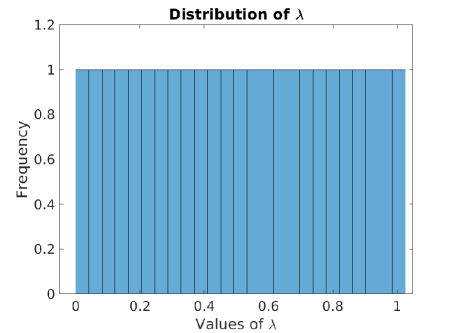
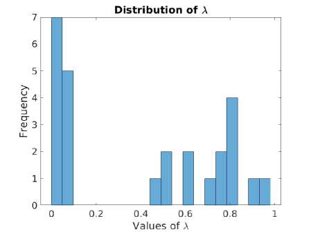
Figure 2: Test 1. Distribution of the sampled values $\mathbb{\lambda}$.

A similar behavior is obtained when the discretization in $\lambda$ is refined. In Fig. 3 the updating constant $\delta$ is $\delta=10^{-4}$ and $N_{\mathbb{\lambda}}=54$.

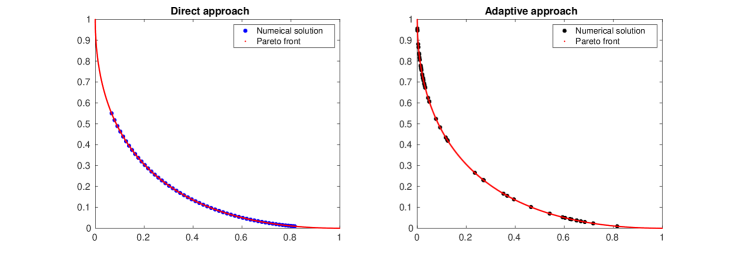
Figure 3: Test 1. Numerical approximation of the Pareto front, with the direct approach (left) and the adaptive approach (right). The red line is the exact Pareto front.

Focusing on the direct approach, Fig. 3 (left), we notice that even for a larger number of values $N_{\lambda}$ the whole Pareto front is not covered.

This graphical interpretation is also compared quantitatively. Given a parametrization of the Pareto front and an equispaced grid, we consider the sum of the minimal distance $d$ between each point of the grid, $x_{i}$ for $i=1,\dots,N_{g}$ with $N_{g}>0$, and the mean of the ensembles at terminal time for different values of $N_{\mathbb{\lambda}}$

$$\frac{\sum_{i=1}^{N_{g}}\min d(x_{i},u^{*}(\mathbb{\lambda}))}{N_{g}}$$ (60)

The measure (60) is similar to the notion of performance metric (IGD) described in [27]. The comparison shows the improved performance of the adaptive approach for increasing number $N_{\lambda}$ as expected, see Fig. 4.

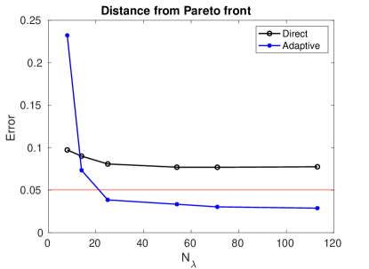
Figure 4: Test 1. The distance from the Pareto front computed by (60) is shown for different number of points, for the direct approach (black) and for the adaptive one (blue). The red line indicates the resolution of the Pareto front given by $N_{g}$.

3.4 Test 2: Non-Convex Case

We consider two non convex functions $\mathcal{G}_{1}$ and $\mathcal{G}_{2}$ defined by

$$\mathcal{G}_{1}(u)=1-e^{-(u-1)^{2}}\qquad\mathcal{G}_{2}(u)=1-e^{-(u+1)^{2}}.$$ (61)

and an initial ensemble $U_{0}\sim\mathcal{U}(-2,2)$ of size $J=50$, and $\delta=1\cdot 10^{-3}$ leading to $N_{\mathbb{\lambda}}=64$. The comparison between the two approaches is shown on $S_{G}$ in Fig. 5. The behavior is similar to the previous case and shows the improvement of the adaptive approach compared with the direct approach.

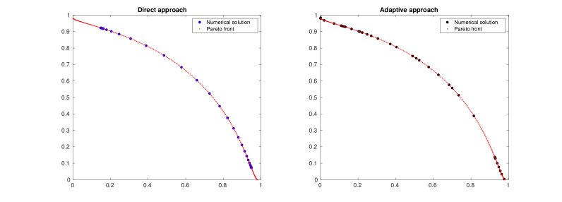
Figure 5: Test 2: Numerical approximation of the Pareto front in the non-convex case, with the direct approach (left) and the adaptive approach (right). The red line is the exact Pareto front.

3.5 Test 3: Multi-dimensional Parameter Space

We consider $\mathcal{G}_{1},\mathcal{G}_{2}$ two convex functions on $\mathbb{R}^{2}$ and given by

$$\mathcal{G}_{1}(u_{1},u_{2})=5(u_{1}-0.1)^{2}+(u_{2}-0.1)^{2}\qquad\mathcal{G}_{2}(u_{1},u_{2})=(u_{1}-0.9)^{2}+5(u_{2}-0.9)^{2}.$$ (62)

The initial ensemble is chosen uniformly distributed $U_{0}\sim\mathcal{U}([0,1]^{2})$ and we consider $J=30$ particles. We set $\delta=8\cdot 10^{-4}$ and $N_{\mathbb{\lambda}}=68$. A similar behavior as before is observed in Fig. 6. However, the approximation to $S_{G}$ does not match completely the analytically solution, especially in the region at $x=2.$ It is assumed that this is due to the terminal time and we refer to Fig. 6-7 where $T_{fin}=50.$ Furthermore, we show the approximation to the set of Pareto points $S_{U}$ in Fig. 9. The adaptive choice of sampling $\Lambda$ leads to a relatively sharp resolution of the set $S_{U}$ compared with the direct approach. The later produces a cloud of points compared to the clusters obtained with the adaptive strategy.

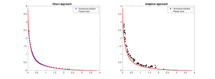
Figure 6: Test 3. Numerical approximation of the Pareto front, with the direct approach(left) and the adaptive approach (right) at $T_{fin}=5$. The red line is the analytical Pareto front.

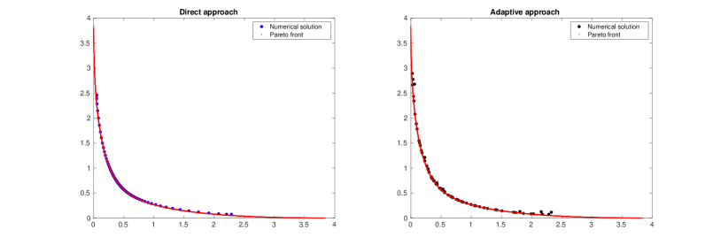
Figure 7: Test 3. Numerical approximation of the Pareto front, with the direct approach(left) and the adaptive approach (right) at $T_{fin}=50$. The red line is the analytical Pareto front.

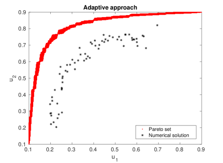
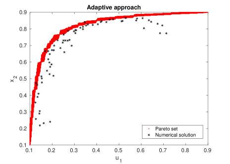
Figure 8: Test 3: Numerical approach of the Pareto set for the adaptive approach for $T_{fin}=5$ (left) and $T_{fin}=50$ (right).

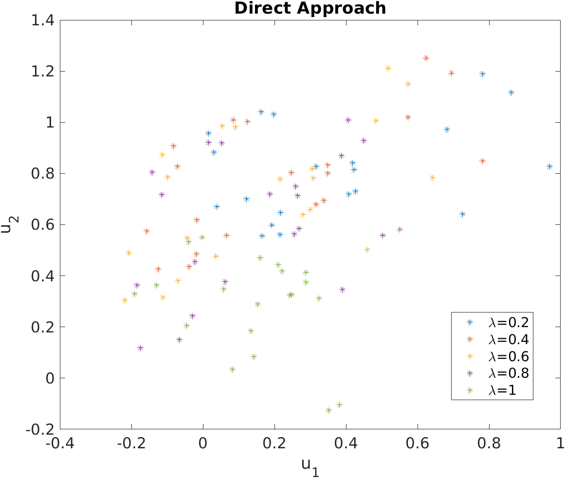
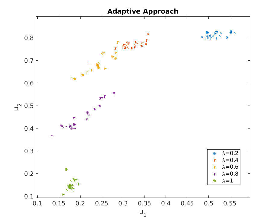
Figure 9: Test 3: Ensemble distribution at $T_{fin}=50$ for different values of $\mathbb{\lambda}$ indicated by color.

4 Summary

The ensemble Kalman filter method has been extended to solve coupled inverse problems. The link to a multi–objective optimization problem has been shown and the analytical properties of the ensemble based method have been investigated. In particular, the mean field equation and their corresponding moment system have been presented and exploited to develop a new adaptive approach for sampling the Pareto front. Numerical results show the improvement of the adaptive strategy also in the nonlinear case.

Acknowledgments

The authors thank the Deutsche Forschungsgemeinschaft (DFG, German Research Foundation) for the financial support through 20021702/GRK2326, 333849990/IRTG-2379, HE5386/19-2,22-1,23-1 and under Germany’s Excellence Strategy EXC-2023 Internet of Production 390621612.

References

- [1] S. I. Aanonsen, G. Nævdal, D. S. Oliver, A. C. Reynolds, and B. Vallès, The ensemble kalman filter in reservoir engineering–a review, Spe Journal, 14 (2009), pp. 393–412.
- [2] D. Blömker, C. Schillings, and P. Wacker, A strongly convergent numerical scheme from ensemble kalman inversion, SIAM Journal on Numerical Analysis, 56 (2018), pp. 2537–2562.
- [3] D. Blömker, C. Schillings, P. Wacker, and S. Weissmann, Well posedness and convergence analysis of the ensemble kalman inversion, Inverse Problems, 35 (2019), p. 085007.
- [4] S. Boyd, S. P. Boyd, and L. Vandenberghe, Convex optimization, Cambridge university press, 2004.
- [5] J. Carrillo and U. Vaes, Wasserstein stability estimates for covariance-preconditioned fokker–planck equations, Nonlinearity, 34 (2021), p. 2275.
- [6] J. A. Carrillo, M. Fornasier, G. Toscani, and F. Vecil, Particle, kinetic, and hydrodynamic models of swarming, in Mathematical modeling of collective behavior in socio-economic and life sciences, Springer, 2010, pp. 297–336.
- [7] N. K. Chada, C. Schillings, and S. Weissmann, On the incorporation of box-constraints for ensemble kalman inversion, Foundations of Data Science, 1 (2019), p. 433.
- [8] N. K. Chada, A. M. Stuart, and X. T. Tong, Tikhonov regularization within ensemble kalman inversion, SIAM Journal on Numerical Analysis, 58 (2020), pp. 1263–1294.
- [9] K. Deb, S. Bandaru, and H. Seada, Generating uniformly distributed points on a unit simplex for evolutionary many-objective optimization, in International Conference on Evolutionary Multi-Criterion Optimization, Springer, 2019, pp. 179–190.
- [10] Z. Ding and Q. Li, Ensemble kalman inversion: mean-field limit and convergence analysis, Statistics and Computing, 31 (2021), pp. 1–21.
- [11] M. Ehrgott, Multicriteria optimization, vol. 491, Springer Science & Business Media, 2005.
- [12] H. W. Engl, M. Hanke, and A. Neubauer, Regularization of inverse problems, vol. 375, Springer Science & Business Media, 1996.
- [13] G. Evensen, Sequential data assimilation with a nonlinear quasi-geostrophic model using monte carlo methods to forecast error statistics, Journal of Geophysical Research: Oceans, 99 (1994), pp. 10143–10162.
- [14] A. Garbuno-Inigo, F. Hoffmann, W. Li, and A. M. Stuart, Interacting langevin diffusions: Gradient structure and ensemble kalman sampler, SIAM Journal on Applied Dynamical Systems, 19 (2020), pp. 412–441.
- [15] M. Herty and G. Visconti, Kinetic methods for inverse problems, Kinetic & Related Models, 12 (2019), p. 1109.
- [16] , Continuous limits for constrained ensemble kalman filter, Inverse Problems, 36 (2020), p. 075006.
- [17] M. A. Iglesias, Iterative regularization for ensemble data assimilation in reservoir models, Computational Geosciences, 19 (2015), pp. 177–212.
- [18] T. Janjić, D. McLaughlin, S. E. Cohn, and M. Verlaan, Conservation of mass and preservation of positivity with ensemble-type kalman filter algorithms, Monthly Weather Review, 142 (2014), pp. 755–773.
- [19] S. I. Kabanikhin and O. I. Krivorotko, Coupled inverse problems and visualization of atmosphere-ocean system, in COUPLED VI: proceedings of the VI International Conference on Computational Methods for Coupled Problems in Science and Engineering, CIMNE, 2015, pp. 921–929.
- [20] A. J. Majda and X. T. Tong, Performance of ensemble kalman filters in large dimensions, Communications on Pure and Applied Mathematics, 71 (2018), pp. 892–937.
- [21] K. Miettinen, Nonlinear multiobjective optimization, vol. 12, Springer Science & Business Media, 2012.
- [22] P. M. Pardalos, A. Žilinskas, J. Žilinskas, et al., Non-convex multi-objective optimization, Springer, 2017.
- [23] L. Pareschi and G. Toscani, Interacting multiagent systems: kinetic equations and Monte Carlo methods, OUP Oxford, 2013.
- [24] C. Schillings and A. M. Stuart, Analysis of the ensemble kalman filter for inverse problems, SIAM Journal on Numerical Analysis, 55 (2017), pp. 1264–1290.
- [25] M. Schwenzer, G. Visconti, M. Ay, T. Bergs, M. Herty, and D. Abel, Identifying trending model coefficients with an ensemble kalman filter–a demonstration on a force model for milling, IFAC-PapersOnLine, 53 (2020), pp. 2292–2298.
- [26] N.-Z. Sun and W. W.-G. Yeh, Coupled inverse problems in groundwater modeling: 1. sensitivity analysis and parameter identification, Water resources research, 26 (1990), pp. 2507–2525.
- [27] Q. Zhang, A. Zhou, S. Zhao, P. N. Suganthan, W. Liu, S. Tiwari, et al., Multiobjective optimization test instances for the cec 2009 special session and competition, University of Essex, Colchester, UK and Nanyang technological University, Singapore, special session on performance assessment of multi-objective optimization algorithms, technical report, 264 (2008), pp. 1–30.