11email: huyinlin@gmail.com, {firstname.lastname}@epfl.ch
Perspective Flow Aggregation for
Data-Limited 6D Object Pose Estimation
Abstract
Most recent 6D object pose estimation methods, including unsupervised ones, require many real training images. Unfortunately, for some applications, such as those in space or deep under water, acquiring real images, even unannotated, is virtually impossible. In this paper, we propose a method that can be trained solely on synthetic images, or optionally using a few additional real ones. Given a rough pose estimate obtained from a first network, it uses a second network to predict a dense 2D correspondence field between the image rendered using the rough pose and the real image and infers the required pose correction. This approach is much less sensitive to the domain shift between synthetic and real images than state-of-the-art methods. It performs on par with methods that require annotated real images for training when not using any, and outperforms them considerably when using as few as twenty real images.
Keywords:
6D Object Pose Estimation, 6D Object Pose Refinement, Image Synthesis, Dense 2D Correspondence, Domain Adaptation1 Introduction
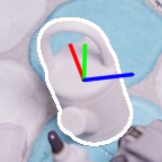
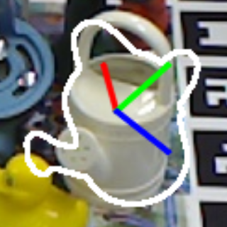
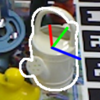
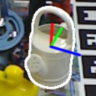
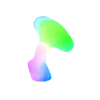
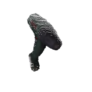
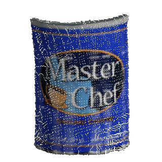
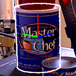
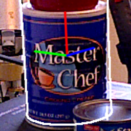
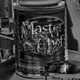
Estimating the 6D pose of a target object is at the heart of many robotics, quality control, augmented reality applications, among others. When ample amounts of annotated real images are available, deep learning-based methods now deliver excellent results [7, 32, 31, 46, 38]. Otherwise, the most common approach is to use synthetic data instead [25, 49, 14]. However, even when sophisticated domain adaptations techniques are used to bridge the domain gap between the synthetic and real data [34, 26, 14], the results are still noticeably worse than when training with annotated real images, as illustrated by Fig. 1.
Pose refinement offers an effective solution to this problem: An auxiliary network learns to correct the mistakes made by the network trained on synthetic data when fed with real data [33, 25, 51, 23]. The most common refinement strategy is to render the object using the current pose estimate, predict the 6D difference with an auxiliary network taking as input the rendered image and the input one, and correct the estimate accordingly. As illustrated by Fig. 2(a), this process is performed iteratively. Not only does this involve a potentially expensive rendering at each iteration, but it also is sensitive to object occlusions and background clutter, which cannot be modeled in the rendering step. Even more problematically, most of these methods still require numerous real images for training purposes, and there are applications for which such images are simply not available. For example, for 6D pose estimation in space [20, 14] or deep under water [17, 36], no real images of the target object may be available, only a CAD model and conjectures about what it now looks like after decades in a harsh environment. These are the scenarios we will refer to as data-limited.
 |
 |
 |
 |
 |
| (a) | (b) | (c) | (d) | (e) |
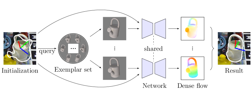
To overcome these problems, we introduce the non-iterative pose refinement strategy depicted by Fig. 2(b). We again start from a rough initial pose but, instead of predicting a delta pose, we estimate a dense 2D correspondence field between the image rendered with the initial pose and the input one. We then use these correspondences to compute the 6D correction algebraically. Our approach is simple but motivated by the observation that predicting dense 2D-to-2D matches is much more robust to the synthetic-to-real domain gap than predicting a pose difference directly from the image pair, as shown in Fig. 1(d-e). Furthermore, this strategy naturally handles the object occlusions and is less sensitive to the background clutter.
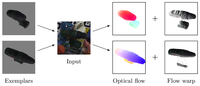
Furthermore, instead of synthesizing images given the rough initial pose, which requires on-the-fly rendering, we find nearest neighbors among pre-rendered exemplars and estimate the dense 2D correspondences between these neighbors and the real input. This serves several purposes. First, it makes the computation much faster. Second, it makes the final accuracy less dependent on the quality of the initial pose, which only serves as a query for exemplars. Third, as multiple exemplars are independent of each other, we can process them simultaneously. Finally, multiple exemplars deliver complementary perspectives about the real input, which we combine for increased robustness.
We evaluate our pose refinement framework on the challenging Occluded-LINEMOD [22] and YCB-V [49] datasets, and demonstrate that it is significantly more efficient and accurate than iterative frameworks. It performs on par with state-of-the-art methods that require annotated real images for training when not using any, and outperforms them considerably when using as few as twenty real images.

|
|
| (a) The iterative strategy | (b) Our non-iterative strategy |
2 Related Work
6D pose estimation is currently dominated by neural network-based methods [11, 32, 38, 37, 14, 2]. However, most of their designs are still consistent with traditional techniques. That is, they first establish 3D-to-2D correspondences [27, 44, 45] and then use a Perspective-n-Points (PnP) algorithm [24, 52, 21, 3]. In practice, these correspondences are obtained by predicting either the 2D locations of predefined 3D keypoints [19, 33, 43, 29, 16], or the 3D positions of the pixels within the object mask [51, 26, 8]. These methods have been shown to outperform those that directly regress the 6D pose [49], which are potentially sensitive to object occlusions. Nevertheless, most of these methods require large amounts of annotated real training data to yield accurate predictions. Here, we propose a pose refinement strategy that allows us to produce accurate pose estimates using only synthetic training data.
6D pose refinement [19, 33, 51, 40] aims to improve an initial rough pose estimate, obtained, for example, by a network trained only on synthetic data. In this context, DeepIM [25] and CosyPose [23] iteratively render the object in the current pose estimate and predict the 6D pose difference between the rendered and input images. However, learning to predict a pose difference directly does not easily generalize to different domains, and these methods thus also require annotated data. Furthermore, the on-the-fly rendering performed at each iteration makes these algorithms computationally demanding. Finally, these methods are sensitive to object occlusions and background clutter, which cannot be modeled in the rendering process. Here, instead, we propose a non-iterative method based on dense 2D correspondences. Thanks to our use of offline-generated exemplars and its non-iterative nature, it is much more efficient than existing refinement methods. Furthermore, it inherently handles occlusions and clutter, and, as we will demonstrate empirically, generalizes easily to new domains. The method in [28] also uses 2D information for pose refinement. Specifically, it iteratively updates the pose so as to align the model’s contours with the image ones. As such, it may be sensitive to the target shape, object occlusion and background clutter. Instead, we use dense pixel-wise correspondences, which are more robust to these disturbances and only need to be predicted once.
Optical flow estimation, which provides dense 2D-to-2D correspondences between consecutive images [35, 13, 15, 12, 39, 42], is a building block of our framework. Rather than estimating the flow between two consecutive video frames, as commonly done by optical flow methods, we establish dense 2D correspondences between offline-generated synthetic exemplars and the real input image. This is motivated by our observation that establishing dense correspondences between an image pair depends more strongly on the local differences between these images, rather than the images themselves, making this strategy more robust to a domain change. This is evidenced by the fact that our network trained only on synthetic data remains effective when applied to real images.
Domain adaptation constitutes the standard approach to bridging the gap between different domains. However, most domain adaptation methods assume the availability of considerable amounts of data from the target domain, albeit unsupervised, to facilitate the adaptation [41, 30, 4, 1]. Here, by contrast, we focus on the scenario where capturing such data is difficult. As such, domain generalization, which aims to learn models that generalize to unseen domains [5], seems more appropriate for solving our task. However, existing methods typically assume that multiple source domains are available for training, which is not fulfilled in our case. Although one can generate many different domains by augmentation techniques [53, 48, 50], we observed this strategy to only yield rough 6D pose estimates in the test domain. Therefore, we use this approach to obtain our initial pose, which we refine with our method.
3 Approach
We aim to estimate the 6D pose of a known rigid object from a single RGB image in a data-limited scenario, that is, with little or even no access to real images during training. To this end, we use a two-step strategy that first estimates a rough initial pose and then refines it. Where we differ from other methods is in our approach to refinement. Instead of using the usual iterative strategy, we introduce a non-iterative one that relies on an optical flow technique to estimate 2D-to-2D correspondences between an image rendered using the object’s 3D model in the estimated pose and the target image. The required pose correction between the rough estimate and the correct one can then be computed algebraically using a PnP algorithm. Fig. 3 depicts our complete framework.
3.1 Data-Limited Pose Initialization
Most pose refinement methods [25, 51, 23] assume that rough pose estimates are provided by another approach trained on a combination of real and synthetic data [49], often augmented in some manner [32, 10, 14]. In our data-limited scenarios, real images may not be available, and we have to rely on synthetic images alone to train the initial pose estimation network.
We will show in the results section that it requires very substantial augmentations for methods trained on synthetic data alone to generalize to real data, and that they only do so with a low precision. In practice, this is what we use to obtain our initial poses.
 |
3.2 From Optical Flow to Pose Refinement
Given an imprecise estimate of the initial pose, we seek to refine it. To this end, instead of directly regressing a 6D pose correction from an image rendered using the pose estimate, we train a network to output a dense 2D-to-2D correspondence field between the rendered image and the target one, that is, to estimate optical flow [42]. From these dense 2D correspondences, we can then algebraically compute the 6D pose correction using a PnP algorithm. In the results section, we will show that this approach generalizes reliably to real images even when trained only on synthetic ones.
More formally, let be the image of the target object and let be the one rendered using the rough pose estimate. We train a network to predict the 2D flow image such that
| (1) |
where contains the indices of the pixels in for which a corresponding pixel in exists, and denote the pixel locations of matching points in both images, and is the corresponding 2D flow vector.
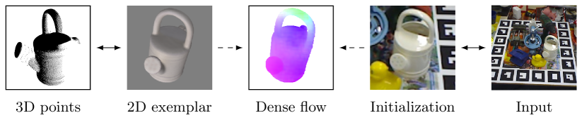
Because has been rendered using a known 6D pose, the 2D image locations are in known correspondence with 3D object points . Specifically, the 3D point corresponding to the 2D location can be obtained by intersecting the camera ray passing through and the 3D mesh model transformed by the initial 6D pose [18], as shown in the left of Fig. 4. For each such correspondence, which we denote as , we have
| (2) |
where is a scale factor encoding depth, is the matrix of camera intrinsic parameters, and and are the rotation matrix and translation vector representing the 6D pose.
To simplify the discussion, let us for now assume that the intrinsic matrix used to render is the same as that of the real camera, which is assumed to be known by most 6D pose estimation methods. We will discuss the more general case in Section 3.4. Under this assumption, the flow vectors predicted for an input image provide us with 2D-to-3D correspondences between the input image and the 3D model. That is, for two image locations deemed to be in correspondence according to the optical flow, we have
| (3) |
Given enough such 3D-to-2D correspondences, the 6D pose in the input image can be obtained algebraically using a PnP algorithm [24]. In other words, we transform the pose refinement problem as a 2D optical flow one, and the 3D-to-2D correspondence errors will depend only on the 2D flow field . Fig. 5 shows an example of dense correspondences between the synthetic and real domains.
 |
 |
 |
 |
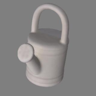
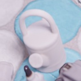
 |
| Exemplar | PBR input | Real input | Prediction | Ground truth |
3.3 Exemplar-Based Flow Aggregation
The above-mentioned flow-based strategy suffers from the fact that it relies on an expensive rendering procedure, which slows down both training and testing. To address this, we use exemplars rendered offline. Instead of synthesizing the image from the initial pose directly, which requires on-the-fly rendering, we then retrieve the exemplar with 6D pose nearest to the initial pose estimate and compute the 2D displacements between this exemplar and the input image.
The resulting speed increase comes at the cost of a slight accuracy loss. However, it is compensated by the fact that this approach enables to exploit multiple rendered views, while only needing a single input image. That is, we do not use a single exemplar but multiple ones rendered from different viewpoints to make our pose refinement more robust. During inference, we use the initial pose to find the closest exemplars and combine their optical flow. In short, instead of having one set of 3D-to-2D correspondences, we now have such sets, which we write as
| (4) |
where is the number of correspondences found for exemplar . Because the exemplars may depict significantly different viewpoints, this allows us to aggregate more information and adds both robustness and accuracy, as depicted by Fig. 6. Finally, we use a RANSAC-based PnP algorithm [24] to derive the final pose based on these complementary correspondences.
3.4 Dealing with Small Objects
In practice, even when using multiple exemplars, the approach described above may suffer from the fact that estimating the optical flow of small objects is challenging. To tackle this, inspired by other refinement methods [25, 51, 23], we work on image crops around the objects. Specifically, because we know the ground-truth pose for the exemplars and have a rough pose estimate for the input image, we can define 2D transformation matrices and that will map the object region in the exemplar and in the input image to a common size. We can then compute the flow between the resulting transformed images.
Formally, let be an exemplar 2D image location after transformation. Furthermore, accounting for the fact that the intrinsic camera matrices used to render the exemplars and acquire the input image may differ, let be an input image location after transformation, where is the intrinsic matrix used for the exemplars and the one corresponding to the input image. We then estimate a flow field using the flow network. For two transformed image locations found to be in correspondence, following the discussion in Section 3.2, we can establish 3D-to-2D correspondences in the transformed image as
| (5) |
We depict this procedure in Fig. 4. We can then recover the corresponding in the original input image by applying the inverse transformation, which then lets us combine the correspondences from multiple exemplars.
3.5 Implementation Details
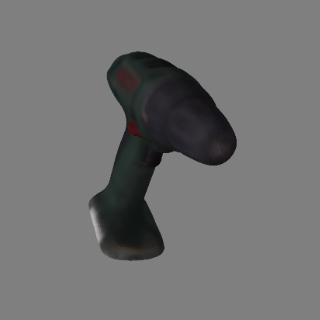
We use the WDR-Pose network [14] as our initialization network, and RAFT [42] as our 2D correspondence network. We first train WDR-Pose on the BOP synthetic data [7, 9], which contains multiple rendered objects and severe occlusions in each frame to simulate real images. Before training the flow network, we generate a set of exemplars for each object type by offline rendering. To avoid computing a huge set of exemplars by densely sampling the 6D pose space, we fix the 3D translation and randomly sample a small set of 3D rotations. Specifically, we set the 3D translation to , where is approximately the average depth of the working range. In our experiments, we found that 10K exemplars for each object type yields a good accuracy. We generate our exemplar images using the method of [18] with a fixed light direction pointing from the camera center to the object center.
To build image pairs to train the flow network, we pick one image from the exemplar set and the other from the BOP synthetic dataset. Specifically, we query the closest exemplar in terms of 6D pose. To simulate the actual query process, we first add some pose jitter to the target instance. Specifically we add a random rotation angle within 20 degrees and a random translation leading to a reprojection offset smaller than 10 pixels. Note that this randomness only affects the query procedure; it does not affect the supervision of the flow network, which relies on the selected exemplar and the synthetic image.
In practice, to account for small objects, we first extract the object instances from the exemplar and target images using the transformation matrices and discussed above. We then resize the resulting object crops to and build the ground-truth flow according to Eq. 5. We only supervise the flow of pixels located within the exemplar’s object mask. Furthermore, during training, we also discard all pixels without explicit correspondence because of occlusions or because they fall outside the crops.
Finally, during training, we apply two main categories of data augmentation techniques. The first is noise (NS) augmentation. We add a random value between -25 to 25 to the pixels in each image channel. We then blur the resulting image with a random kernel size between 1 and 5. The second is color (HSV) augmentation. We convert the input image from RGB to HSV and add random jitter to each channel. Specifically, we add 20%, 50%, 50% of the maximum value of each channel as the random noise to the H, S, and V channel, respectively. We then convert the image back to RGB.
4 Experiments
In this section, we first compare our approach to the state of the art on standard datasets including LINEMOD (“LM”) [6], Occluded-LINEMOD (“OLM”) [22] and YCB-V (“YCB”) [49]. We then evaluate the influence of different components of our refinement network. We defer the evaluation of the initialization network trained only on synthetic data to Section 4.3. The source code is publicly available at https://github.com/cvlab-epfl/perspective-flow-aggregation.
Datasets and Experimental Settings. LINEMOD comprises 13 sequences. Each one contains a single object annotated with the ground-truth pose. There are about 1.2K images for each sequence. We train our model only on the exemplars and the BOP synthetic dataset, and test it on 85% of the real LINEMOD data as in [33, 25]. We keep the remaining 15% as supplementary real data for our ablation studies. Occluded-LINEMOD has 8 objects, which are a subset of the LINEMOD ones. It contains only 1214 images for testing, with multiple objects in the same image and severe occlusions, making it much more challenging.
Most methods train their models for LINEMOD and Occluded-LINEMOD separately [11, 26], sometimes even one model per object [32, 47], which yields better accuracy but is less flexible and does not scale well. As these two datasets share the same 3D meshes, we train a single model for all 13 objects and test it on LINEMOD and Occluded-LINEMOD without retraining. When testing on Occluded-LINEMOD, we only report the accuracy of the corresponding 8 objects. We show that our model still outperforms most methods despite this generalization that makes it more flexible.
YCB-V is a more recent dataset that contains 92 video sequences and about 130K real images depicting 21 objects in cluttered scenes with many occlusions and complex lighting conditions. As for LINEMOD, unless stated otherwise, we train our model only on the exemplars and the BOP synthetic dataset and test on the real data.
Evaluation metrics. We compute the 3D error as the average distance between 3D points on the object surface transformed by the predicted pose and by the ground-truth one. We then report the standard ADD-0.1d metric [49], that is, the percentage of samples whose 3D error is below 10% of the object diameter. For more detailed comparisons, we use ADD-0.5d, which uses a larger threshold of 50%. Furthermore, to compare with other methods on YCB-V, we also report the AUC metric as in [32, 23, 47], which varies the threshold with a maximum of 10cm and accumulates the area under the accuracy curve. For symmetric objects, the 3D error is taken to be the distance of each 3D point to its nearest model point after pose transformation.
| Data | Metrics | PoseCNN | SegDriven | PVNet | GDR-Net | DeepIM | CosyPose | Ours (+0) | Ours (+20) |
|---|---|---|---|---|---|---|---|---|---|
| LM | ADD-0.1d | 62.7 | - | 86.3 | 93.7 | 88.6 | - | 84.5 | 94.4 |
| OLM | ADD-0.1d | 24.9 | 27.0 | 40.8 | 62.2 | 55.5 | - | 48.2 | 64.1 |
| YCB | ADD-0.1d | 21.3 | 39.0 | - | 60.1 | - | - | 56.4 | 62.8 |
| AUC | 61.3 | - | 73.4 | 84.4 | 81.9 | 84.5 | 76.8 | 84.9 |
4.1 Comparison with the State of the Art
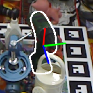
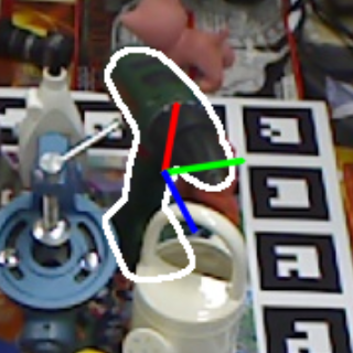
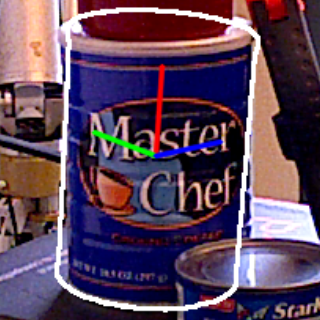
We now compare our method to the state-of-the-art ones, PoseCNN [49], SegDriven [11], PVNet [32], GDR-Net [47], DeepIM [25], and CosyPose [23], where DeepIM and CosyPose are two refinement methods based on an iterative strategy. We train our initialization network WDR-Pose only on synthetic data and use its predictions as initial poses. To train the optical flow network, we generate 10K exemplars for each object and use the closest exemplars during inference. As shown in Table 1, even without accessing any real images during training, our method already outperforms most of the baselines, which all use real training data, and performs on par with the most recent ones. Fig. 7 depicts some qualitative results. Note that YCB-V contains some inaccurate pose annotations, and, as shown in Fig. 8, we sometimes predict more accurate poses than the annotations, even when training without accessing any real data.
In Table 1, we also report the results we obtain by adding 20 real images to the synthetic ones during the training of our refinement network. In this case, we train each model by mixing the BOP synthetic data with the real images, balancing their ratio to be 0.5:0.5 by dynamic sampling during training. Note that we still use the same pose initializations trained only on synthetic images. With only 20 real images, our method outperforms all the baselines by a significant margin, even though they all use all the real images during training.
 |
 |
 |
 |
 |
 |
 |
 |
 |
 |
| Initializations | Exemplars | Predicted flow | Forward warp | Refinements |
 |
 |
 |
 |
| Annotation | Reprojection | Difference | Our result |
| 0 | 10 | 20 | 90 | 180 | |
|---|---|---|---|---|---|
| DeepIM | 41.1 | 45.6 | 48.2 | 58.1 | 61.4 |
| CosyPose | 42.4 | 46.8 | 48.9 | 58.8 | 61.9 |
| Ours | 48.2 | 59.5 | 64.1 | 64.9 | 65.3 |
Most existing refinement methods, including DeepIM and CosyPose, employ pose initializations trained using all real images, which is impractical in our data-limited scenario. To have a fair comparison of our refinement method with them, we use the same synthetic-only pose initializations for them as for our approach. We then train the refinement networks according to their open-source official code, based on synthetic data only. Furthermore, we also evaluate them when trained with different numbers of additional real images. Note that, while CosyPose can use multiple views as input, we only evaluate it in the monocular case to make it comparable with the other methods. In Table 2, we report the ADD-0.1d on the challenging Occluded-LINEMOD dataset. As expected, using more real images yields more accurate pose estimates for all methods. However, with as few as 20 real images, our model achieves even higher accuracy than the baselines with more than 100 real images. Since all methods use the same initial poses, giving an accuracy of 37.9%, as shown in Table 5, this means that DeepIM and CosyPose can only increase the initialization accuracy by 3-4% when not accessing any real image data. By contrast, our method increases accuracy by over 10% in this case, demonstrating the robustness of our method to the domain gap in cluttered scenarios.
4.2 Ablation Studies
Let us now analyze more thoroughly the exemplar-based flow aggregation in our pose refinement framework. To this end, we conduct more ablation studies on the standard LINEMOD dataset. We train our refinement model only on synthetic data [9], and report ADD-0.1d accuracies on real test data.
Flow Aggregation. We first evaluate our flow aggregation strategy given different pose initializations. We use three initialization sets with varying levels of accuracy, corresponding to the results from the initialization network under NS, HSV, and NS+HSV augmentations, respectively. Furthermore, we evaluate the accuracy using different numbers of retrieved exemplars, also reporting the corresponding running speed on a typical workstation with a 3.5G CPU and an NVIDIA V100 GPU.
| Initialization | =1 | =2 | =4 | =8 | |
|---|---|---|---|---|---|
| NS | 54.1 | 82.0 | 82.7 | 84.3 | 84.1 |
| HSV | 52.7 | 81.1 | 81.2 | 83.3 | 83.9 |
| NS+HSV | 60.2 | 82.0 | 83.4 | 84.5 | 84.9 |
| FPS | 32 | 25 | 20 | 14 | |
As shown in Table LABEL:tab:flow_aggregation, the refinement network improves the accuracy of the initial pose significantly even with only one exemplar. More exemplars boost it further, thanks to the complementarity of their different viewpoints. Interestingly, although the different pose initializations have very different pose accuracies, they all reach a similar accuracy after our pose refinement, demonstrating the robustness of our refinement network to different initial poses. As the exemplars can be processed in parallel, the running time with 4 exemplars is only about 1.6 slower than that with a single exemplar. This slight speed decrease is related to the throughput of the GPU and could be optimized further in principle. Nevertheless, our approach is still more than 3 times faster than the iterative DeepIM [25] method, which runs at only about 6 FPS using 4 iterations. Since the version with 8 exemplars yields only a small improvement over the one with 4 exemplars, we use =4 in the previous experiments. Furthermore, we use the results of NS+HSV for pose initialization.
Exemplar Set. While using an exemplar set eliminates the need for online rendering, the accuracy of our approach depends on its granularity, leading to a tradeoff between accuracy and IO storage/speed. We therefore evaluate the performance of our approach with varying numbers of exemplars during inference. To better understand the query process, we also report the numbers just after the query but before the refinement, denoted as “Before Ref.”.
Table LABEL:tab:exemplar_set_size shows that larger exemplar sets yield more accurate queries before the refinement, leading to more accurate pose refinement results. Note that because we have a discrete set of exemplars, the ADD-0.1d scores before refinement are lower than those obtained by on-the-fly rendering from the initial pose, which reaches 60.2%. While fewer exemplars in the set translates to lower accuracy before refinement, the accuracy after refinement saturates beyond 10K exemplars, reaching a similar performance to online rendering. We therefore use 10K exemplars for each object in the previous experiments. This only requires about 200MB of disk space for storing the exemplar set for each object. We also report the timings of image preparation for each setting. Although there is a powerful GPU for the online rendering, our offline exemplar retrieval is much faster.
| 2.5K | 5K | 10K | 20K | 40K | Online | |
|---|---|---|---|---|---|---|
| Before Ref. | 55.2 | 57.0 | 58.0 | 58.9 | 59.9 | 60.2 |
| After Ref. | 81.9 | 83.2 | 84.5 | 85.0 | 84.8 | 84.9 |
| Image preparation | 16ms | 19ms | 29ms | 52ms | 81ms | 184ms |
4.3 Pose Initialization Network
We now evaluate our pose initialization network based on WDR-Pose [14]. Unlike in [14], we train it only on the BOP synthetic data [7, 9] and study the performance on real images. To fill the domain gap between the synthetic and real domains, we use simple data augmentation strategies during training.
Specifically, we evaluate 3 groups of data augmentations. The first one consists of random shifts, scales, and rotations within a range of (-50px, 50px), (0.9, 1.1), and (-45∘, 45∘), respectively. We refer to this as SSR augmentations. The second group incudes random noise and smoothness, and corresponds to the NS augmentations discussed in Section 4.2. The final group performs color augmentations, and corresponds to the HSV augmentations presented in Section 4.2.
| Data | Metrics | No | SSR | NS | HSV | NS+HSV |
|---|---|---|---|---|---|---|
| LM | ADD-0.1d | 48.9 | 39.0 | 56.6 | 58.1 | 60.2 |
| ADD-0.5d | 93.2 | 80.7 | 98.8 | 97.0 | 98.9 | |
| OLM | ADD-0.1d | 28.6 | 20.9 | 36.0 | 34.4 | 37.9 |
| ADD-0.5d | 74.8 | 69.2 | 83.0 | 81.3 | 86.1 | |
| YCB | ADD-0.1d | 0.1 | 0 | 17.0 | 7.4 | 27.5 |
| ADD-0.5d | 2.9 | 0 | 59.0 | 36.6 | 72.3 |
Table 5 summarizes the results of the model trained with these different data augmentations on LINEMOD, Occluded-LINEMOD, and YCB-V. We report the accuracy in terms of both ADD-0.1d and ADD-0.5d. In short, training on synthetic data without data augmentation (“No”) yields poor performance on the real test data, with an accuracy of almost zero in both metrics on the YCB-V dataset. Interestingly, although the NS and HSV augmentations can considerably increase the performance, the SSR augmentations degrade it consistently on all three datasets. We believe this to be due to the geometric nature of the SSR augmentations. More precisely, after shifting, scaling, or rotating the input image, the resulting inputs do not truly correspond to the original 6D poses, which inevitably introduces errors in the learning process. However, the NS and HSV augmentations do not suffer from this problem, as the ground-truth annotations before and after augmentation are the same.
Note that, although the NS and HSV augmentations significantly outperform no augmentation, the accuracy remains rather low in terms of ADD-0.1d. However, the ADD-0.5d numbers evidence that most of the predictions have an error of less than 50% of the diameter of the object. This indicates that the resulting rough initialization can indeed serve as a good starting point for our pose refinements, as demonstrated before.
5 Conclusion
We have introduced a simple non-iterative pose refinement strategy that can be trained only on synthetic data and yet still produce good results on real images. It relies on the intuition that, using data augmentation, one can obtain a rough initial pose from a network trained on synthetic images, and that this initialization can be refined by predicting dense 2D-to-2D correspondences between an image rendered in approximately the initial pose and the input image. Our experiments have demonstrated that our approach yields results on par with the state-of-the-art methods that were trained on real data, even when we don’t use any real images, and outperforms these methods when we access as few as 20 images. In other words, our approach provides an effective and efficient strategy for data-limited 6D pose estimation. Nevertheless, our method remains a two-stage framework, which may limit its performance. In the future, we will therefore investigate the use of a differentiable component to replace RANSAC PnP and make our method end-to-end trainable.
Acknowledgments. This work was supported by the Swiss Innovation Agency (Innosuisse). We would like to thank Sébastien Speierer and Wenzel Jakob in EPFL Realistic Graphics Lab (RGLab) for the helpful discussions on rendering.
References
- [1] Cui, S., Wang, S., Zhuo, J., Su, C., Huang, Q., Tian, Q.: Gradually Vanishing Bridge for Adversarial Domain Adaptation. In: Conference on Computer Vision and Pattern Recognition (2020)
- [2] Di, Y., Manhardt, F., Wang, G., Ji, X., Navab, N., Tombari, F.: SO-Pose: Exploiting Self-Occlusion for Direct 6D Pose Estimation. In: International Conference on Computer Vision (2021)
- [3] Ferraz, L., Binefa, X., Moreno-Noguer, F.: Very Fast Solution to the PnP Problem with Algebraic Outlier Rejection. In: Conference on Computer Vision and Pattern Recognition. pp. 501–508 (2014)
- [4] Gu, X., Sun, J., Xu, Z.: Spherical Space Domain Adaptation with Robust Pseudo-Label Loss. In: Conference on Computer Vision and Pattern Recognition (2020)
- [5] Gulrajani, I., Lopez-Paz, D.: In Search of Lost Domain Generalization. In: International Conference on Learning Representations (2021)
- [6] Hinterstoisser, S., Lepetit, V., Ilic, S., Holzer, S., Bradski, G., Konolige, K., Navab, N.: Model Based Training, Detection and Pose Estimation of Texture-Less 3D Objects in Heavily Cluttered Scenes. In: Asian Conference on Computer Vision (2012)
- [7] Hoda, T., Michel, F., Brachmann, E., Kehl, W., Buch, A.G., Kraft, D., Drost, B., Vidal, J., Ihrke, S., Zabulis, X., Sahin, C., Manhardt, F., Tombari, F., Kim, T.K., Matas, J., Rother, C.: BOP: Benchmark for 6D Object Pose Estimation. In: European Conference on Computer Vision (2018)
- [8] Hodan, T., Barath, D., Matas, J.: EPOS: Estimating 6D Pose of Objects with Symmetries. In: Conference on Computer Vision and Pattern Recognition (2020)
- [9] Hodan, T., Vineet, V., Gal, R., Shalev, E., Hanzelka, J., Connell, T., Urbina, P., Sinha, S., Guenter, B.: Photorealistic Image Synthesis for Object Instance Detection. In: International Conference on Image Processing (2019)
- [10] Hu, Y., Fua, P., Wang, W., Salzmann, M.: Single-Stage 6D Object Pose Estimation. In: Conference on Computer Vision and Pattern Recognition (2020)
- [11] Hu, Y., Hugonot, J., Fua, P., Salzmann, M.: Segmentation-Driven 6D Object Pose Estimation. In: Conference on Computer Vision and Pattern Recognition (2019)
- [12] Hu, Y., Li, Y., Song, R.: Robust Interpolation of Correspondences for Large Displacement Optical Flow. In: Conference on Computer Vision and Pattern Recognition (2017)
- [13] Hu, Y., Song, R., Li, Y.: Efficient Coarse-to-Fine PatchMatch for Large Displacement Optical Flow. In: Conference on Computer Vision and Pattern Recognition (2016)
- [14] Hu, Y., Speierer, S., Jakob, W., Fua, P., Salzmann, M.: Wide-Depth-Range 6D Object Pose Estimation in Space. In: Conference on Computer Vision and Pattern Recognition (2021)
- [15] Ilg, E., Mayer, N., Saikia, T., Keuper, M., Dosovitskiy, A., Brox, T.: FlowNet 2.0: Evolution of Optical Flow Estimation with Deep Networks. In: Conference on Computer Vision and Pattern Recognition (2017)
- [16] Jafari, O.H., Mustikovela, S.K., Pertsch, K., Brachmann, E., Rother, C.: IPose: Instance-Aware 6D Pose Estimation of Partly Occluded Objects. In: Asian Conference on Computer Vision (2018)
- [17] Joshi, B., Modasshir, M., Manderson, T., Damron, H., Xanthidis, M., Li, A.Q., Rekleitis, I., Dudek, G.: DeepURL: Deep Pose Estimation Framework for Underwater Relative Localization. In: International Conference on Intelligent Robots and Systems (2020)
- [18] Kato, H., Ushiku, Y., Harada, T.: Neural 3D Mesh Renderer. In: Conference on Computer Vision and Pattern Recognition (2018)
- [19] Kehl, W., Manhardt, F., Tombari, F., Ilic, S., Navab, N.: SSD-6D: Making Rgb-Based 3D Detection and 6D Pose Estimation Great Again. In: International Conference on Computer Vision (2017)
- [20] Kisantal, M., Sharma, S., Park, T.H., Izzo, D., Märtens, M., D’Amico, S.: Satellite Pose Estimation Challenge: Dataset, Competition Design and Results. In: IEEE Transactions on Aerospace and Electronic Systems (2020)
- [21] Kneip, L., Li, H., Seo, Y.: UPnP: An Optimal O(n) Solution to the Absolute Pose Problem with Universal Applicability. In: European Conference on Computer Vision (2014)
- [22] Krull, A., Brachmann, E., Michel, F., Yang, M.Y., Gumhold, S., Rother, C.: Learning Analysis-By-Synthesis for 6D Pose Estimation in RGB-D Images. In: International Conference on Computer Vision (2015)
- [23] Labbé, Y., Carpentier, J., Aubry, M., Sivic, J.: CosyPose: Consistent Multi-View Multi-Object 6D Pose Estimation. In: European Conference on Computer Vision (2020)
- [24] Lepetit, V., Moreno-Noguer, F., Fua, P.: EPnP: An Accurate O(n) Solution to the PnP Problem. International Journal of Computer Vision (2009)
- [25] Li, Y., Wang, G., Ji, X., Xiang, Y., Fox, D.: DeepIM: Deep Iterative Matching for 6D Pose Estimation. In: European Conference on Computer Vision (2018)
- [26] Li, Z., Wang, G., Ji, X.: CDPN: Coordinates-Based Disentangled Pose Network for Real-Time Rgb-Based 6-DoF Object Pose Estimation. In: International Conference on Computer Vision (2019)
- [27] Lowe, D.G.: Distinctive Image Features from Scale-Invariant Keypoints. International Journal of Computer Vision 20(2), 91–110 (November 2004)
- [28] Manhardt, F., Kehl, W., Navab, N., Tombari, F.: Deep Model-Based 6D Pose Refinement in RGB. In: European Conference on Computer Vision (2018)
- [29] Oberweger, M., Rad, M., Lepetit, V.: Making Deep Heatmaps Robust to Partial Occlusions for 3D Object Pose Estimation. In: European Conference on Computer Vision (2018)
- [30] Pan, F., Shin, I., Rameau, F., Lee, S., Kweon, I.: Unsupervised Intra-Domain Adaptation for Semantic Segmentation through Self-Supervision. In: Conference on Computer Vision and Pattern Recognition (2020)
- [31] Park, K., Patten, T., Vincze, M.: Pix2Pose: Pixel-Wise Coordinate Regression of Objects for 6D Pose Estimation. In: International Conference on Computer Vision (2019)
- [32] Peng, S., Liu, Y., Huang, Q., Zhou, X., Bao, H.: PVNet: Pixel-Wise Voting Network for 6DoF Pose Estimation. In: Conference on Computer Vision and Pattern Recognition (2019)
- [33] Rad, M., Lepetit, V.: BB8: A Scalable, Accurate, Robust to Partial Occlusion Method for Predicting the 3D Poses of Challenging Objects Without Using Depth. In: International Conference on Computer Vision (2017)
- [34] Rad, M., Oberweger, M., Lepetit, V.: Feature Mapping for Learning Fast and Accurate 3D Pose Inference from Synthetic Images. In: Conference on Computer Vision and Pattern Recognition (2018)
- [35] Revaud, J., Weinzaepfel, P., Harchaoui, Z., Schmid, C.: EpicFlow: Edge-Preserving Interpolation of Correspondences for Optical Flow. In: Conference on Computer Vision and Pattern Recognition (2015)
- [36] Risholm, P., Ivarsen, P.O., Haugholt, K.H., Mohammed, A.: Underwater Marker-Based Pose-Estimation with Associated Uncertainty. In: International Conference on Computer Vision (2021)
- [37] Sock, J., Garcia-Hernando, G., Armagan, A., Kim, T.K.: Introducing Pose Consistency and Warp-Alignment for Self-Supervised 6D Object Pose Estimation in Color Images. In: International Conference on 3D Vision (2020)
- [38] Song, C., Song, J., Huang, Q.: HybridPose: 6D Object Pose Estimation Under Hybrid Representations. In: Conference on Computer Vision and Pattern Recognition (2020)
- [39] Sun, D., Yang, X., Liu, M., Kautz, J.: PWC-Net: CNNs for Optical Flow Using Pyramid, Warping, and Cost Volume. In: Conference on Computer Vision and Pattern Recognition (2018)
- [40] Sundermeyer, M., Durner, M., Puang, E.Y., Marton, Z.C., Vaskevicius, N., Arras, K.O., Triebel, R.: Multi-Path Learning for Object Pose Estimation Across Domains. In: Conference on Computer Vision and Pattern Recognition (2020)
- [41] Tang, H., Chen, K., Jia, K.: Unsupervised Domain Adaptation via Structurally Regularized Deep Clustering. In: Conference on Computer Vision and Pattern Recognition (2020)
- [42] Teed, Z., Deng, J.: RAFT: Recurrent All-Pairs Field Transforms for Optical Flow. In: European Conference on Computer Vision (2020)
- [43] Tekin, B., Sinha, S.N., Fua, P.: Real-Time Seamless Single Shot 6D Object Pose Prediction. In: Conference on Computer Vision and Pattern Recognition (2018)
- [44] Tola, E., Lepetit, V., Fua, P.: DAISY: An Efficient Dense Descriptor Applied to Wide Baseline Stereo. IEEE Transactions on Pattern Analysis and Machine Intelligence 32(5), 815–830 (2010)
- [45] Trzcinski, T., Christoudias, C.M., Lepetit, V., Fua, P.: Learning Image Descriptors with the Boosting-Trick. In: Advances in Neural Information Processing Systems (December 2012)
- [46] Wang, C., Xu, D., Zhu, Y., Martín-Martín, R., Lu, C., Fei-Fei, L., Savarese, S.: DenseFusion: 6D Object Pose Estimation by Iterative Dense Fusion. In: Conference on Computer Vision and Pattern Recognition (2019)
- [47] Wang, G., Manhardt, F., Tombari, F., Ji, X.: GDR-Net: Geometry-Guided Direct Regression Network for Monocular 6D Object Pose Estimation. In: Conference on Computer Vision and Pattern Recognition (2021)
- [48] Wang, Z., Luo, Y., Qiu, R., Huang, Z., Baktashmotlagh, M.: Learning to Diversify for Single Domain Generalization. In: International Conference on Computer Vision (2021)
- [49] Xiang, Y., Schmidt, T., Narayanan, V., Fox, D.: PoseCNN: A Convolutional Neural Network for 6D Object Pose Estimation in Cluttered Scenes. In: Robotics: Science and Systems Conference (2018)
- [50] Xu, Q., Zhang, R., Zhang, Y., Wang, Y., Tian, Q.: A Fourier-Based Framework for Domain Generalization. In: Conference on Computer Vision and Pattern Recognition (2021)
- [51] Zakharov, S., Shugurov, I., Ilic, S.: DPOD: 6D Pose Object Detector and Refiner. In: International Conference on Computer Vision (2019)
- [52] Zheng, Y., Kuang, Y., Sugimoto, S., Åström, K., Okutomi, M.: Revisiting the PnP Problem: A Fast, General and Optimal Solution. In: International Conference on Computer Vision (2013)
- [53] Zhou, K., Yang, Y., Qiao, Y., Xiang, T.: Domain Generalization with Mixstyle. In: International Conference on Learning Representations (2021)