Representative Subset Selection for Efficient Fine-Tuning
in Self-Supervised Speech Recognition

Abstract

Self-supervised speech recognition models require considerable labeled training data for learning high-fidelity representations for Automatic Speech Recognition (ASR) which is computationally demanding and time-consuming. We consider the task of identifying an optimal subset of data for efficient fine-tuning in self-supervised speech models for ASR. We discover that the dataset pruning strategies used in vision tasks for sampling the most informative examples do not perform better than random subset selection on fine-tuning self-supervised ASR. We then present the Cowerage algorithm for representative subset selection in self-supervised ASR. Cowerage is based on our finding that ensuring the coverage of examples based on training Word Error Rate (WER) in the early training epochs leads to better generalization performance. Extensive experiments with the wav2vec 2.0 and HuBERT model on TIMIT, Librispeech, and LJSpeech datasets show the effectiveness of Cowerage and its transferability across models, with up to 17% relative WER improvement over existing dataset pruning methods and random sampling. We also demonstrate that the coverage of training instances in terms of WER values ensures the inclusion of phonemically diverse examples, leading to better test accuracy in self-supervised speech recognition models.

1 Introduction

There has been rapid progress in recent years toward improving speech self-supervised learning (speech SSL) models. Such models learn high-fidelity speech representations using a large amount of unlabeled data and use paired data for fine-tuning on the downstream task of automatic speech recognition (ASR) (Baevski et al., 2020; Hsu et al., 2021). However, still a significant amount of labeled training data is used in the fine-tuning step, which is computationally demanding and time-consuming. For example, the standard wav2vec2 fine-tuning procedure on Librispeech/Libri-light requires $\sim$$50$$-$$100$ hours on a V100 GPU, which is significantly higher ($>50\times$) than the cost of fine-tuning BERT on GLUE (Lai et al., 2021). Moreover, this also hinders their usage in low-resource systems, especially compute-restricted environments (e.g., cheaper GPUs and on-device computing), which is presently a significant barrier in democratizing access to these models (Ahmed & Wahed, 2020; Paul et al., 2021).

Recent work uses adapters to enable efficient fine-tuning by using a fraction of parameters in speech SSL models (Thomas et al., 2022). However, their usage necessitates task-specific modifications, which prevents their applicability across different models and datasets. In contrast, we consider increasing the efficiency of speech SSL fine-tuning procedure by reducing training data requirements and find smaller, representative and model-agnostic subsets of data for fine-tuning speech SSL models. Finally, we consider how example diversity within optimal subsets affects generalization in speech SSL, which is an important theoretical question requiring further investigation.

The data pruning mechanisms specifically tailored for deep learning models have been studied extensively for standard vision tasks. These methods focus on selecting the most informative training examples (Toneva et al., 2018; Coleman et al., 2019; Paul et al., 2021; Raju et al., 2021; Karamcheti et al., 2021; Margatina et al., 2021; Mindermann et al., 2022) which has been shown to perform better than the random selection of the training data. The methods for identifying the important examples in these cases are based on scores that are directly derived from the training properties and example difficulty such as the error vector norm (Paul et al., 2021), the number of times an example is forgotten during training (Toneva et al., 2018) or the holdout loss (Mindermann et al., 2022). However, no such mechanism has been studied yet for data pruning in speech SSL models.

Studying the impact of the data subset selection on ASR model performance raises several questions: Can we identify a model-agnostic scoring method based on the training properties for dataset pruning in speech SSL without significantly sacrificing the test accuracy? What are the phoneme distributions of good subsets of training data, and how do they affect the latent representations within speech SSL models? Can we analyze the training landscape of speech SSL and extract novel insights that can benefit other speech tasks? The answers to these questions will help construct representative subsets that will benefit the paradigm of optimal dataset construction.

We find that in standard datasets for training speech SSL models, sampling only the hard-to-learn training examples based on word error rate (WER) does not consistently perform better than random pruning. This is in contrast to data pruning strategies in vision tasks where this method outperforms other baselines (Toneva et al., 2018; Paul et al., 2021; Sorscher et al., 2022). For better data subset selection in fine-tuning speech SSL models, we propose Cowerage, an algorithm designed to identify training examples important for better generalization. We find that ensuring the coverage of diverse examples based on training WER values in the early training epochs leads to better accuracy on unseen test data than random pruning or selecting only the most informative (hard-to-learn) examples. Experiments show the effectiveness of the Cowerage algorithm over three primary pruning strategies: random selection, top k (hardest subset selection), and bottom k (easiest subset selection). To understand the underlying mechanism governing Cowerage’s generalization properties, we establish a connection between the training WER of the examples and their phonemic cover and find that our algorithm ensures the inclusion of phonemically diverse examples (i.e., examples of both low and high phonemic coverage) without explicitly learning any phoneme-level error model. Finally, we demonstrate that phonemic diversity affects discrete latent representation within speech SSL, leading to performance gains via Cowerage subset selection.

1.1 Our Contributions

• We use the WER of the individual training examples as the basis for subset selection algorithms that prune the training data for speech SSL models (Section 3).

• We present Cowerage, an algorithm for selecting a subset of ASR training data that ensures uniform coverage of training WER values via a stratified random sampling approach (Section 3.3).

• Empirical evaluation on two models — wav2vec2 (Baevski et al., 2020) and HuBERT (Hsu et al., 2021) — across three speech datasets — TIMIT (Garofolo et al., 1993), Librispeech (Panayotov et al., 2015) and LJSpeech (Ito & Johnson, 2017) — show that fine-tuning on the subset selected by Cowerage gives a lower WER on the test split as compared to three other pruning strategies: random, top k, and bottom k examples (Section 5). Additionally, we demonstrate that the subsets constructed through one model can be used for fine-tuning another speech SSL model, i.e., they are transferable (Section 5.1).

• We study the properties of the subsets selected by Cowerage by examining the phonemic coverage of training examples. We find that by ensuring the coverage of training WER values, Cowerage is able to select phonemically diverse examples, which results in a richer training subset (Section 6). Finally, we establish the relationship between phonemic diversity and the discrete latent representation within speech SSL which allows Cowerage to perform better than random subset selection and hardest/easiest example selection (Section 6.1).

2 Preliminaries

Consider a self-supervised model $f(x;\theta)$ ($\theta\in\mathcal{R}^{d}$) that is pre-trained on a large unlabelled dataset $x\in\mathcal{D}_{u}$ on some objective $\mathcal{L}_{p}$. The model obtained after self-supervised pretraining with weights $\theta_{L}$ is then fine-tuned for the downstream task of ASR with another objective $\mathcal{L}_{f}$ on a labelled dataset $x\in\mathcal{D}_{l}$ (which is generally smaller than $\mathcal{D}_{u}$). $\mathcal{D}_{l}$ consists of transcribed audios (i.e. audio and the corresponding sentence that was uttered). Our goal is to prune $\mathcal{D}_{l}$ to obtain a subset ${B}_{l}$ such that the performance of self-supervised ASR model $f(x;\theta)$ after fine-tuning on ${B}_{l}$ is better than random pruning. We only consider pruning $\mathcal{D}_{l}$ (and not ${D}_{u}$) since we aim to directly evaluate the impact of different subset selection methods on the downstream task of ASR instead of the unsupervised pre-training of speech SSL model. The performance of an ASR model is commonly evaluated via WER ($\frac{I+D+S}{N}$), which is computed by aligning the word sequence generated by the ASR system with the actual transcription (containing N words) and calculating the sum of substitutions (S), insertions (I), and deletions (D) (Woodard & Nelson, 1982).

3 Method

A number of active learning approaches are based on the inclusion of informative training examples in the dataset for deep learning models, i.e., examples with high error during the training epochs. Such examples have been found to have a greater influence on learning how to correctly label the remaining training data and thus are considered more important than examples with low error (easier examples). We first quantify the importance of a training example in the context of a self-supervised ASR system to form a baseline for the comparison of different pruning algorithms. The training WER of an example after a few training epochs is representative of the difficulty of that example in being transcribed correctly by an ASR system. Intuitively, a hard-to-learn example will have a higher training WER due to the greater misalignment between the generated word sequence and the actual transcription. We now use the training WER to present three different subset selection strategies for selecting a subset ${B}_{l}$ of the training data ${D}_{l}$ for fine-tuning a self-supervised speech model on ASR.

3.1 Strategy 1: Picking the hardest k examples

The first approach is to pick the top $k$ training examples, i.e., the ones with the highest WER (Algorithm 1). This replicates the pruning strategy of picking the highest error examples (Paul et al., 2021; Margatina et al., 2021) during training. We first compute the training WER in a particular epoch (WER selection epoch) for all the examples. Then we select examples with the highest WER and perform fine-tuning on this subset. The number of examples selected is determined by the pruning fraction p.

3.2 Strategy 2: Picking the easiest k examples

The second strategy is to pick the bottom $k$ training examples i.e., the ones with the lowest WER (Algorithm 1). This is the inverse of strategy 3.1 and removes the harder-to-learn outliers from the training set in an attempt to retain representative examples.

Algorithm 1 Top k and Bottom k Example Selection for fine-tuning ASR Model

1:Input: SSL Pretrained Model $f$, Dataset ${D}_{l}$, Strategy $s$ (Top k / Bottom k), Pruning Fraction $p$, Training Epoch $e$

2:$W\leftarrow$ Fine-tune $f$ on ${D}_{l}$ and compute WER for each example on epoch $e$

3:$retainFraction\leftarrow$ $1-p$

4:$retainSize\leftarrow retainFraction*len({D}_{l})$

5:if $s=\text{Top {k}}$ then

6:     $W\leftarrow sortDescending(W)$

7:else

8:     $W\leftarrow sortAscending(W)$

9:end if

10:${B}_{l}\leftarrow W[0:retainSize]$

3.3 Strategy 3: Cowerage Subset Selection

Algorithm 2 Cowerage Subset Selection for fine-tuning ASR Model

1:Input: SSL Pretrained Model $f$, Dataset ${D}_{l}$, Pruning Fraction $p$, Training Epoch $e$, Bucket Size $b$

2:$W\leftarrow$ Finetune $f$ on ${D}_{l}$ and compute WER for each example on epoch $e$

3:$retainFraction\leftarrow$ $1-p$

4:${B}_{l}\leftarrow\emptyset$

5:$W\leftarrow sortDescending(W)$

6:$buckets\leftarrow createBuckets(W,size=b)$

7:for $bucket$ in $buckets$ do

8:     $sampleSize\leftarrow retainFraction*b$

9:     $S\leftarrow randomSample(bucket,sampleSize)$

10:     ${B}_{l}\leftarrow{B}_{l}\cup S$

11:end for

We now present a novel approach for dataset pruning, which we call Cowerage, i.e., picking examples to ensure the coverage of the training WER. The following claim forms the basis of the Cowerage algorithm, which we prove later through multiple experiments (Section 5).

Claim 3.1.

Ensuring the coverage of training WER values guarantees the inclusion of phonemically diverse examples in the training data.

With Cowerage, we first compute the training WER for each example in ${D}_{l}$, with the lowest WER as $w_{l}$ and the highest WER as $w_{h}$. We then use a stratified sampling approach of partitioning $N$ total examples from the range $[w_{l},w_{h}]$ into $M$ buckets, with each bucket defined as,

where $i=1\ldots n$. We then use simple random sampling to select $k$ examples uniformly from each bucket,

$$X_{1,\ldots,}X_{k}\sim\mathcal{U}\left(S_{i}\right)$$ (2)

where $k$ is decided by the fraction of the dataset to be pruned and the size of the bucket. $\mathcal{U}\left(S_{i}\right)$ denotes the uniform distribution over the set $S_{i}$. This stratified sampling method ensures coverage of WER when selecting training examples. The selected subset is used to fine-tune speech SSL model for ASR and the test performance is evaluated through WER (Fig. 1). The overall algorithm is presented in Algorithm 2.

Our method requires an initial fine-tuning run to compute the ranking of examples, similar to other supervised pruning methods, e.g., EL2N scores (Paul et al., 2021), RHO-LOSS (Mindermann et al., 2022) and Forgetting Norm (Azeemi et al., 2022). However, this subset is transferable and can subsequently be used for fine-tuning multiple ASR models (Section 5.1). This amortizes the initial cost of complete training run across the efficiency improvements achieved via multiple fine-tunings done using the created subset. Sorscher et al. (2022) identify such pruned datasets as foundation datasets which can be used for multiple downstream tasks.

3.3.1 Comparison to Random Sampling

We now highlight the key differences between random subset selection and Cowerage.

Claim 3.2.

In contrast to the Cowerage algorithm, random sampling does not ensure selection of examples from the tail WER range.

Proof.

We consider the probability of randomly selecting an example WER ($w$) that is at least at a distance of $k$ standard deviation $\sigma$ from the mean WER. By Chebyshev’s inequality: $\operatorname{Pr}(|X-\bar{W}|\geq k\sigma)\leq\frac{1}{k^{2}}=p$, which demonstrates that increasing the WER boundary $w$ (and hence $k$) decreases the probability of randomly selecting a sample with WER greater than $w$. We now consider the probability of having at least one sample with a WER greater $w$ when we independently draw $n$ samples from the training WER distribution. This is a complement of the event no sample having a WER greater than $w$ in $n$ draws which is $(1-p)^{n}$, and hence the event of interest has the probability upper bound $1-(1-p)^{n}=1-(1-\frac{1}{k^{2}})^{n}$. This demonstrates that decreasing the sample size and increasing the pruning percentage reduces the probability of selecting a tail WER example. In contrast, for Cowerage, the probability of selecting at least one example with a WER greater than $\bar{W}+k\sigma$ is $Pr(|S_{i}|>0)=q$, where $S_{i}$ is a tail bucket with the WER range $(a,b)$ such that $a\geq\bar{W}+k\sigma$ and $b>a$. This probability ($q$) approaches 1 if we consider a bucket size satisfying the range $(a,b)$, and hence Cowerage ensures selection of examples from the tail WER range.

∎

Claim 3.3.

Subsets selected by Cowerage have a lower variance of the sample mean of WER than randomly selected samples.

Proof.

We first consider the variance of samples selected by Cowerage. Let $S_{ij}$ be the sample $i$ from bucket $S_{j}$. The average WER in bucket $j$ is $\bar{W}_{j}=\frac{\sum_{i}S_{ij}}{k}$, variance in bucket $j$ is $\sigma_{j}^{2}$ and the overall average is $\bar{W}=\frac{\sum_{j}\bar{W}_{j}}{M}$. The variance of the sample mean of WER is,

$$\mathrm{Var}_{\textsc{cowerage}}[\bar{W}]=\frac{\sum_{j}\mathrm{Var}\left[\bar{W}_{j}\right]}{M^{2}}$$ (3)

$\mathrm{Var}\left[\bar{W}_{j}\right]$ is the variance of the sample mean within a particular bucket and is equivalent to $\frac{\sigma_{j}^{2}}{k}$. Thus, we get

Now we consider the variance of a simple random sample. $\mathrm{Var}[\bar{W}]=\frac{\sigma^{2}}{N}$ with $\sigma^{2}=\mathbb{E}\left[W^{2}\right]-\mu^{2}$. Considering the contribution from each bucket in the random sample, we can specify $\sigma^{2}=\frac{\sum_{j}\mathbb{E}\left[S_{j}\right]}{M}-\mu^{2}=\frac{\sum_{j}\left(\mu_{j}^{2}+\sigma_{j}^{2}\right)}{M}-\mu^{2}=\frac{\sum_{j}\left(\left(\mu_{j}-\mu\right)^{2}+\sigma_{j}^{2}\right)}{M}$. Thus,

$$\mathrm{Var_{\textsc{random}}}[\bar{W}]=\frac{\sum_{j}\left(\left(\mu_{j}-\mu\right)^{2}+\sigma_{j}^{2}\right)}{MN}$$ (5)

Comparing (4) and (5), $\mathrm{Var_{\textsc{random}}}[\bar{W}]\geq\mathrm{Var_{\textsc{cowerage}}}[\bar{W}]$ and the result follows.

∎

Figure 1: A conceptual representation of the complete flow for fine-tuning a self-supervised model for ASR using a data subset selected by the Cowerage algorithm. In step (1), we perform fine-tuning on the downstream ASR task using the complete dataset and calculate the training WER on a certain epoch. In step (2), we use Cowerage to create a data subset by bucketing the training WER and selecting a subset of examples from each bucket. We then use this data in step (3) to fine-tune the complete model and then evaluate on the test dataset.

Table 1: Test WER for the four strategies of pruning the training set evaluated at multiple pruning fractions (0.1, 0.3, 0.5, 0.7, 0.9) and different datasets (LJSpeech, LS-10h and TIMIT). The training WER in a particular epoch is averaged over 10 runs and then used for a particular pruning strategy. For each result, we do three independent runs and report the mean test WER. The standard deviation is reported in Table 9. Cowerage consistently demonstrates the lowest WER at various pruning fractions. WER selection epoch (WSE) is set to 8 for these experiments. See Section B.1 for WSE ablation.

Dataset	Strategy	wav2vec2-base						HuBERT-base
		No pruning	0.1	0.3	0.5	0.7	0.9	No pruning	0.1	0.3	0.5	0.7	0.9
LJSpeech	Random	0.052	0.062	0.071	0.085	0.128	0.251	0.091	0.117	0.128	0.140	0.196	0.272
	Top K	0.052	0.060	0.064	0.077	0.101	0.238	0.091	0.109	0.118	0.135	0.168	0.248
	Bottom K	0.052	0.057	0.063	0.070	0.091	0.166	0.091	0.105	0.116	0.130	0.151	0.181
	Cowerage	0.052	0.054	0.060	0.067	0.085	0.144	0.091	0.101	0.107	0.115	0.136	0.153
LS-10h	Random	0.140	0.147	0.168	0.188	0.245	0.360	0.180	0.219	0.220	0.298	0.309	0.424
	Top K	0.140	0.143	0.155	0.174	0.198	0.343	0.180	0.210	0.215	0.268	0.313	0.391
	Bottom K	0.140	0.146	0.159	0.175	0.201	0.336	0.180	0.215	0.219	0.269	0.336	0.381
	Cowerage	0.140	0.142	0.150	0.164	0.192	0.277	0.180	0.185	0.211	0.250	0.290	0.341
TIMIT	Random	0.315	0.325	0.341	0.357	0.394	0.557	0.328	0.357	0.373	0.392	0.452	0.675
	Top K	0.315	0.322	0.334	0.392	0.472	0.678	0.328	0.345	0.366	0.435	0.532	0.871
	Bottom K	0.315	0.336	0.360	0.411	0.521	0.887	0.328	0.346	0.391	0.447	0.568	0.931
	Cowerage	0.315	0.320	0.333	0.339	0.369	0.455	0.328	0.335	0.355	0.381	0.445	0.616

4 Configurations

4.1 Models

We use the wav2vec2-base (Baevski et al., 2020) (95M parameters) and HuBERT-base model (Hsu et al., 2021) (90M parameters) for our experiments. wav2vec2 consists of a CNN-based encoder that processes the input waveform which is then discretized via the quantization layer and passed to the BERT module where the actual contextual representation is learned. HuBERT learns a combined language and acoustic model through a prediction loss which is applied to masked regions only. We select wav2vec2-base and HuBERT-base that is pre-trained on Librispeech 960h, and fine-tune them for ASR using the Connectionist Temporal Classification (CTC) loss (Graves et al., 2006) on the subsets of three speech datasets: TIMIT (Garofolo et al., 1993), Librispeech 10h (Panayotov et al., 2015) and LJSpeech (Ito & Johnson, 2017). We report WER for pruning fractions of 0.1, 0.3, 0.5, 0.7, and 0.9 to adequately evaluate low, moderate, and extreme pruning settings across different strategies. Please see Appendix A.3 for details about train and test splits and Appendix A.4 for hyperparameters.

4.2 Baseline

We consider the baseline experiment of randomly pruning the train split of the dataset on multiple fractions and fine-tuning the ASR model on the generated subset. The performance evaluation is done through WER on the test set.

5 Empirical Evaluation

Experiments. We fine-tune wav2vec2-base model on the selected dataset and calculate the WER of the training examples over ten independent runs. The training scores (averaged over 10 runs) from a particular epoch are then used to prune the examples through the pruning strategies (3.1, 3.2, 3.3) to generate a subset of training data. The data subsets are then used to fine-tune wav2vec2-base and HuBERT-base for ASR. The training WER distribution and the subsets of TIMIT, Librispeech and LJSpeech selected through each method are shown in Appendix B.2.

Results. We show the results of pruning experiments via different strategies across multiple pruning fractions in Table 1. For each strategy and pruning fraction, we report the mean WER of three independent runs. The variability across runs is shown in Appendix 9. We observe that for the majority of pruning fractions, Cowerage subset selection is consistently better than the other three pruning strategies (top k, bottom k, and random pruning) for TIMIT, LS-10h, and LJSpeech. At higher pruning fractions, the difference between the test WER for Cowerage and the other pruning strategies increases, e.g., on the Librispeech-10h dataset with 90% pruning, Cowerage shows 17% relative WER improvement over Bottom K strategy compared to 5% relative WER improvement at 30% pruning. This observation can also be made for random sampling and is consistent with claim 3.2 where we consider the impact of smaller sample sizes (higher pruning percentages) on the selection of examples from tail WER which subsequently affects test error. On the TIMIT dataset, going from 10% pruning to 90% pruning leads to an absolute increase of only 0.135 WER for Cowerage compared to an increase of 0.551, 0.356, and 0.232 for Bottom K, Top K, and Random respectively.

5.1 Transferability of representative subsets

Table 1 shows that Cowerage demonstrates better performance in the fine-tuning run of HuBERT-base on the subsets constructed through training WER values of wav2vec2-base. The relative trend for other pruning strategies is also similar to that of wav2vec2-base. This suggests that the representative subsets computed through one speech SSL model are transferable to another speech SSL model, making them model-agnostic and dataset-specific. We also verify this transferability for a larger model (wav2vec2-large) and the results are shown in Appendix B.5. This property is present in a few other pruning metrics for deep learning models as well, including EL2N score (Paul et al., 2021) and RHO-loss (Mindermann et al., 2022). Our explanation is that since the composition of the representative subset is more influenced by the ranking of training examples instead of absolute WER values (line 5-6 of Algorithm 2), it makes them relevant for fine-tuning other speech SSL models. Additionally, the prior averaging of the training WER values theoretically eliminates the influence of specific model weights, which produces a more precise ranking of the examples. We can consider the representative subsets constructed through Cowerage as foundation datasets (Sorscher et al., 2022) which need to be constructed once and can be later used to fine-tune multiple other speech SSL models.

5.2 Ablation study

The Impact of Offset. To identify whether there is another contiguous subset of examples below the ones with the highest WER which can perform better than random pruning, we introduce an offset while selecting the top k training examples, mirroring the protocol presented by Paul et al. (2021). We compute the training WER for the examples and sort them in ascending order. We then maintain a sliding window from offset $k$ to $k+N$ which keeps $N$ data points but incrementally excludes the training examples with the highest WER. For offset sizes from 0 to 500, we notice a change in the test WER but no single offset size is consistently better than random pruning. An important implication of this finding is that no contiguous subset of training examples picked according to the WER is better than random pruning in the TIMIT speech corpus, contrary to the previous studies on vision datasets that have shown a clear correlation between the top-scoring examples and the accuracy (Paul et al., 2021).

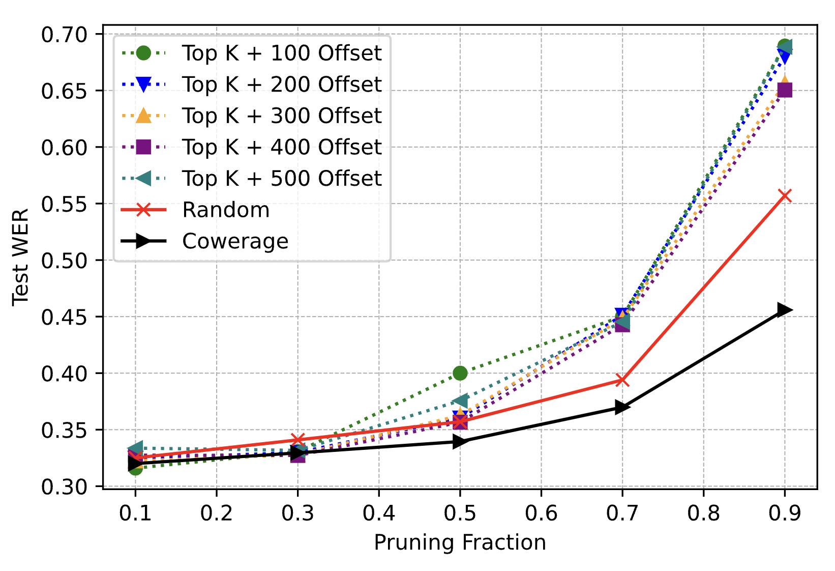
Figure 2: The test WER for the different offsets while picking the top k examples compared over different pruning fractions of the TIMIT dataset. Note that no single offset consistently performs better than random pruning.

Selection within the buckets. The strategy proposed in the original Cowerage algorithm is to randomly sample elements from each bucket. We also evaluate two other strategies: picking the first k examples within each bucket and picking the last k ones, similar to strategies 1 and 2 except that now we are sampling within a particular bucket. The results in Table 2 show that the random selection outperforms other strategies. Additionally, we evaluate the impact of increasing the bucket size on the test WER in Appendix B.4.

Table 2: Test WER for different strategies of picking samples within each bucket for Cowerage algorithm on 0.7 pruning fraction and WER Selection Epoch 8.

	Cowerage + Top k	Cowerage + Bottom k	Cowerage + Random
WER	$0.378\pm 0.002$	$0.401\pm 0.002$	$0.369\pm 0.004$

5.3 Phoneme Recognition on TIMIT

We evaluate the subset selection methods on the task of phoneme recognition with wav2vec2-base on TIMIT dataset and report the phoneme error rate (PER) on the test set (Table 8). Cowerage consistently demonstrates the lowest PER on all the pruning fractions above 0.2.

Table 3: Phoneme recognition on the TIMIT dataset with wav2vec2-base. We report PER for multiple pruning fractions and different strategies.

Strategy	Pruning Fraction
	0.1	0.3	0.5	0.7	0.9
Random	0.124	0.133	0.148	0.230	1.000
Top K	0.118	0.137	0.168	0.244	1.000
Bottom K	0.122	0.142	0.170	0.282	1.000
Cowerage	0.120	0.133	0.145	0.211	1.000

5.4 Training time for subsets

Practically, the choice of pruning fraction can be made according to the intended size of the final dataset under the given time and memory constraints. We conduct an experiment to determine the total steps required for convergence and the real training time for wav2vec2 on TIMIT. The results are shown in Table 4 (for a constant learning rate). We report the real training time for the pruned datasets as a fraction of the training time for the complete dataset ($x$) for relative comparison. There is a significant reduction in training time for higher pruning fractions.

Table 4: Steps required for convergence and training time for wav2vec2 on TIMIT for different pruning fractions. We replicate the results of Cowerage from Table 1 for relative comparison.

Pruning Fraction	0.9	0.7	0.5	0.3	0.1	0
Steps required for convergence	1050	1900	2400	2800	3170	3350
Training time	$0.42\times$	$0.62\times$	$0.77\times$	$0.85\times$	$0.90\times$	$\times$
Test WER (Cowerage)	0.455	0.369	0.339	0.333	0.320	0.315

6 Connection to Phonemes

To understand why Cowerage performs better than other pruning strategies, it is important to find out how does the phoneme distribution of training examples vary with the training error during fine-tuning of the self-supervised speech recognition models. We now perform empirical analysis to verify claim 3.1. For this analysis, we select the standard TIMIT dataset as it contains time-aligned, hand-verified phonetic and word transcriptions for each training example.

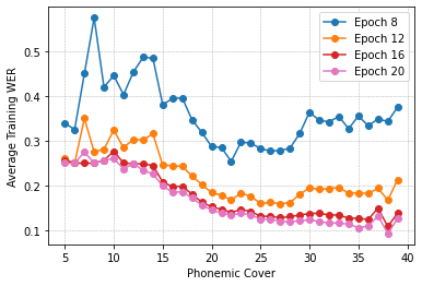
Figure 3: The training WER and the phonemic cover of examples in TIMIT dataset (without pruning) compared over multiple training epochs. The WER is computed by averaging the training scores of the examples with the same phonemic cover. The training scores for each training example and a particular epoch are computed by averaging over 10 runs.

We first record the training WER of each training example in the TIMIT dataset over 10 runs and average it. Then, we compute the total number of unique phonemes in each example, which we call the phonemic cover. Subsequently, we group together the training examples with same phonemic cover and calculate the average training WER for each group (Fig. 3). In the earlier training epochs, the examples with a relatively low ($<17$) or a high ($>28$) phonemic cover have a greater WER (blue line in Fig. 3) as compared to the examples with a moderate number of phonemes ($17\leq\texttt{phonemicCover}\leq 28$). In the later epochs ($\geq 12$), the inverse relationship between the training WER and the phonemic cover becomes more evident; the examples with a greater number of distinct phonemes have a lower training WER and vice versa.

Significance. This relationship between the training WER and the phonemic cover has several implications. Firstly, it demonstrates that there is a sizable population of sentences with a low phonemic cover that are harder to learn and hence represent a high training WER. Similarly, there are many low WER sentences with a high phonemic cover (examples are presented in Appendix B.8). More importantly, this experiment validates our claim that ensuring the coverage of training WER values in a particular subset leads to the inclusion of phonemically diverse training examples without explicitly learning any phoneme-level error model. This is beneficial as accurate phonetic data is not available for the majority of 7000 spoken languages (Billington et al., 2021). In contrast, any method that directly ensures phoneme diversity requires an accurate phonetic transcription beforehand, which is a resource-intensive process requiring manual labeling by linguists.

To verify if the difference between the phoneme distributions of the examples within the Cowerage subset and the other two strategies (top k and bottom k) is statistically significant, we conduct the Mann-Whitney U test, a non-parametric test, at a significance level of 0.01. We found that the differences were statistically significant at the 1% level (p-value $<0.01$). The results are shown in Table 5.

Table 5: The statistical significance of the difference between the phoneme distribution of the examples within the Cowerage subset and the other two strategies (top k and bottom k). MWU: Mann-Whitney U.

	MWU	p-value
Top k vs Cowerage	2146027.5	$<0.001$
Bottom k vs Cowerage	2229653.0	$<0.001$

6.1 Phonemic diversity and latent representation in speech SSL

How does phonemic diversity impact the discrete latent speech representations within self-supervised speech recognition models? To answer this, we study the latent representation ($\mathbf{q}_{t}$) learned by the quantizer within wav2vec2 for different phonemes. Baevski et al. (2020) analyze the conditional probability $P\left(phoneme\mid\mathbf{q}_{t}\right)$ for each of the 39 phonemes in the TIMIT train set by computing the co-occurence between the phonemes and speech latents (see Appendix D of Baevski et al. (2020)). They demonstrate that different discrete latents specialize in different phonetic sounds in wav2vec2 model. Building upon this, Shim et al. (2021) analyze the relationship between attention and phonemes in Transformer-based ASR models by considering the attention map that extracts phonologically meaningful features. They observe that the characteristic feature of phonetic localization is the higher attention weights assigned to similar phonemes in the attention map (see Fig. 3 of Shim et al. (2021)). Given these observations, we hypothesize that the performance gains for Cowerage are due to the greater phonemic diversity which enables a more robust latent representation of each phoneme in wav2vec2. This view is supported by the results in Table 1 which demonstrate bigger gains in test WER for higher pruning fractions in Cowerage. We conjecture that this is due to greater example diversity provided by Cowerage and lack of representation of examples from the tail WER range in the case of other approaches.

7 Related Work

Data pruning. Devising strategies for data pruning and constructing optimal subsets is a recent topic of interest in the area of optimization, coresets and efficient deep learning (Tolochinsky & Feldman, 2018; Dong et al., 2019; Mirzasoleiman et al., 2020; Huang et al., 2021; Jiang et al., 2021; Jubran et al., 2021; Durga et al., 2021; Kothawade et al., 2021; Killamsetty et al., 2021; Kothyari et al., 2021; Azeemi et al., 2022). A few studies have examined the training landscape for drawing clues about the optimal subset creation (Toneva et al., 2018; Agarwal et al., 2020; Baldock et al., 2021; Paul et al., 2021; Schirrmeister et al., 2022). Paul et al. (2021) evaluate the impact of static data pruning on the performance on standard vision datasets (e.g., CIFAR-10 and CIFAR-100) and models (ResNet). They use the gradient norm (GraNd) and the error norm (EL2N) for removing the easy training examples and pruning a significant chunk of the dataset without affecting the generalization error. The authors observe that the local information in the early training epochs is a strong indicator of the importance of training examples and thus can be used to select a good subset of training data effectively. This is consistent with our observation regarding WER selection epoch.

Selection of hard-to-learn examples. Although sampling hard-to-learn examples has been a popular choice for data pruning in deep learning models, it appears to work on a limited set of tasks that share certain properties. A study on visual question answering (VQA) (Karamcheti et al., 2021) demonstrates that the active learning approaches that prefer picking the harder examples do not outperform random pruning on the VQA task across multiple models and datasets. The authors demonstrate the role of collective outliers (Han et al., 2011) in degrading the generalization performance and find out that the preference for selecting these harder-to-learn outliers by the active learning methods is the cause of poor improvements in efficiency as compared to random sampling. Our findings regarding harder-to-learn training examples are similar; they do not consistently perform better for speech SSL models.

Data subset selection for ASR. The existing work on active learning and data pruning for ASR systems emphasize the importance of ensuring phonemically rich text and higher coverage of words (Wu et al., 2007; Ni et al., 2015a; Wei et al., 2014; Mendonça et al., 2014; Ni et al., 2015b, a, 2016). An early study (Wu et al., 2007) demonstrates that selecting a subset that is sampled uniformly across phonemes and words is more effective than random sampling. A subsequent work (Wei et al., 2014) proposes a method for selecting the data by maximizing a constrained sub-modular function. The results show the possibility of a significant reduction of the training data when using acoustic models based on Gaussian mixture models.

In ASR, active learning aims to select the most informative utterances to be transcribed from a large amount of un-transcribed utterances. In contrast, our core objective is to construct an optimal data subset by selecting the informative and representative examples from a fully labeled dataset i.e. the examples for which audios and the reference transcriptions are available.

The majority of these existing approaches have focused on the earlier ASR systems instead of the Deep Neural Network (DNN) based models. Although model pruning has been explored for self-supervised and other ASR models (Lai et al., 2021; Wu et al., 2021; Zhen et al., 2021), data subset selection for fine-tuning self-supervised ASR systems has only been explored in the context of personalization for accented speakers (Awasthi et al., 2021). A phoneme-level error model is proposed which selects sentences that yield a lower test WER as compared to random sentence selection. In contrast, our Cowerage algorithm has the advantage that no complex, dataset-specific phoneme-level error model needs to be learned, which constructs phonemically diverse subsets. Instead, just the training WER can be used to devise a strategy for pruning that performs better than random selection. Additionally, to the best of our knowledge, this is the first study considering data subset selection for efficient fine-tuning in self-supervised speech recognition models.

8 Conclusion and Future Work

In this work, we proposed Cowerage, a new method for pruning data for self-supervised automatic speech recognition, which relies on sampling data in a way that ensures coverage of training WER values. An evaluation on wav2vec2 and HuBERT and three datasets show that Cowerage performs better than random selection and other data pruning strategies that select harder-to-learn or easier-to-learn examples. We demonstrate that the pruned subsets are transferable to other speech SSL models which amortizes the cost of initial training run across the efficiency improvements achieved via multiple fine-tunings done using the created subset. We unveil the connection between the training word error rate and the phonemic cover of training examples across multiple training epochs and analyze the pruning results through this lens. We show that Cowerage outperforms other subset selection strategies as it ensures phonemic diversity within the training examples by directly utilizing the training WER of speech SSL models. While we designed our approach to be dataset agnostic and applicable to different distributions of training WER, it remains to be empirically evaluated whether our methodology generalizes to noisier data and multilingual speech corpora.

Appendix A Implementation Details

A.1 Resources

We use a single 80GB NVIDIA A100 GPU for running all the experiments on the cloud. In this setting, the standard wav2vec2-base fine-tuning step (single run) on multiple pruning fractions took $\approx 1.25$ GPU hours for the TIMIT dataset, $\approx 6$ GPU hours for LJSpeech dataset, and $\approx 5.5$ GPU hours for Librispeech 10h dataset. The total project (from the early experiments to the final results) consumed about 2200 GPU hours.

A.2 Code and Licenses

We release our code under the MIT license. All the data pruning strategies are implemented in Python, and the resulting subsets are used to fine-tune wav2vec2. The publicly available HuggingFace (Wolf et al., 2019) implementation of wav2vec2-base model is used which is based on the standard wav2vec2-base-960h fairseq implementation. The HuggingFace transformers repo is available under the Apache License 2.0 license and the fairseq repo is available under the MIT license.

A.3 Data

TIMIT (Garofolo et al., 1993). We use the full TIMIT dataset with predefined training and test sets. The training set contains 4620 examples and the test set contains 1680 examples. TIMIT is available under the LDC User Agreement for Non-Members.
Librispeech (Panayotov et al., 2015). We construct Librispeech 10h fine-tuning split by selecting 10h of utterances randomly from the 100h train-clean split. The test-clean split is used for evaluation. Librispeech is available under the CC BY 4.0 license.
LJSpeech (Ito & Johnson, 2017). This dataset contains 24 hours of English speech from a single speaker. For validation and testing, we randomly select 300 utterances, mirroring the protocol followed in earlier works (Liu et al., 2022). The rest is used for training. LJSpeech is available under the public domain license.

A.4 Training

In all experiments, wav2vec2-base is fine-tuned with a batch size = 8, epochs = 20, mean ctc-loss-reduction, weight decay 0.005, and FP16 training. We use a data collator to pad the inputs dynamically. For calculating the WER for each training example, we run a computation step after each epoch and record the WER. The training WER in each epoch is averaged over 10 runs and then used for a particular pruning strategy. For each test WER reported, we do three separate runs with independent model initialization. A bucket size of $500$ is chosen for the Cowerage strategy, which is sufficiently small to ensure the selection of representative examples for different pruning fractions.

Appendix B Additional Experiments

B.1 WER Selection Epoch

An important hyperparameter in the Cowerage algorithm is the epoch at which the training WER is computed for individual examples and then used for pruning i.e. the WER selection epoch. We evaluate the effect of different selection epochs on the final test WER (Table 6) in TIMIT and observe that the training WER in the early training epochs can be reliably used for ranking the examples and applying a particular pruning strategy. Hence, we select WSE = 8 for the final results in Table 1. Note that Cowerage consistently demonstrates a lower WER than other strategies on all epochs that we test (8, 12, 16, 20) for the majority of pruning fractions ($0.2-0.9$) across all the datasets (TIMIT, LS-10h, LJSpeech). This suggests that the selection of a reasonable WSE can usually be made with less than five distinct epoch values while still achieving better results than the other strategies.

Table 6: Test WER for the four strategies of pruning the training set evaluated at multiple pruning fractions and different training WER selection epochs. The training WER in a particular selection epoch is averaged over 10 runs and then used for a particular pruning strategy. For each result, we do three independent runs and report the mean test WER. Cowerage consistently demonstrates the lowest WER at various pruning fractions and selection epochs. WSE: WER Selection Epoch.

WSE	Strategy	Pruning Fraction
		No pruning	0.1	0.3	0.5	0.7	0.9
8	Random	0.315	0.325	0.341	0.357	0.394	0.557
	Top K	0.315	0.322	0.334	0.392	0.472	0.678
	Bottom K	0.315	0.336	0.360	0.411	0.521	0.887
	Cowerage	0.315	0.320	0.333	0.339	0.369	0.455
12	Random	0.315	0.325	0.341	0.357	0.394	0.557
	Top K	0.315	0.316	0.345	0.386	0.461	0.579
	Bottom K	0.315	0.323	0.353	0.398	0.499	0.781
	Cowerage	0.315	0.322	0.328	0.354	0.370	0.536
16	Random	0.315	0.325	0.341	0.357	0.394	0.557
	Top K	0.315	0.324	0.332	0.413	0.467	0.704
	Bottom K	0.315	0.323	0.346	0.382	0.468	0.657
	Cowerage	0.315	0.322	0.329	0.356	0.382	0.565
20	Random	0.315	0.324	0.340	0.357	0.401	0.557
	Top K	0.315	0.328	0.370	0.422	0.518	0.709
	Bottom K	0.315	0.321	0.352	0.389	0.457	0.587
	Cowerage	0.315	0.321	0.334	0.340	0.376	0.545

B.2 Training WER Distribution

We compare the distribution of the training WER for TIMIT (Fig. 4), Librispeech 10h (Fig. 5) and LJSpeech (Fig. 6) and show the subsets selected through Top K, Bottom K and Cowerage subset selection on 50% pruning percentage. We notice significant differences in the training WER distribution for the three datasets which highlights that the example difficulty (measured by WER) is a property of the dataset. Moreover, since Cowerage performs better than other subset selection methods across multiple datasets, we hypothesize that the our proposed method is dataset-agnostic and can perform well with different training WER distributions.

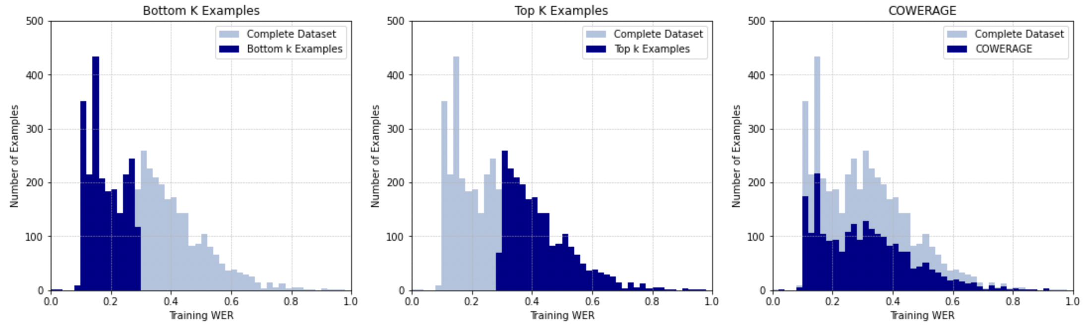
Figure 4: The subset of the TIMIT training data selected by each of the three strategies: bottom k (left), top k (middle) and Cowerage (right). The pruning fraction is set to 0.5 and the WER selection epoch is 8.

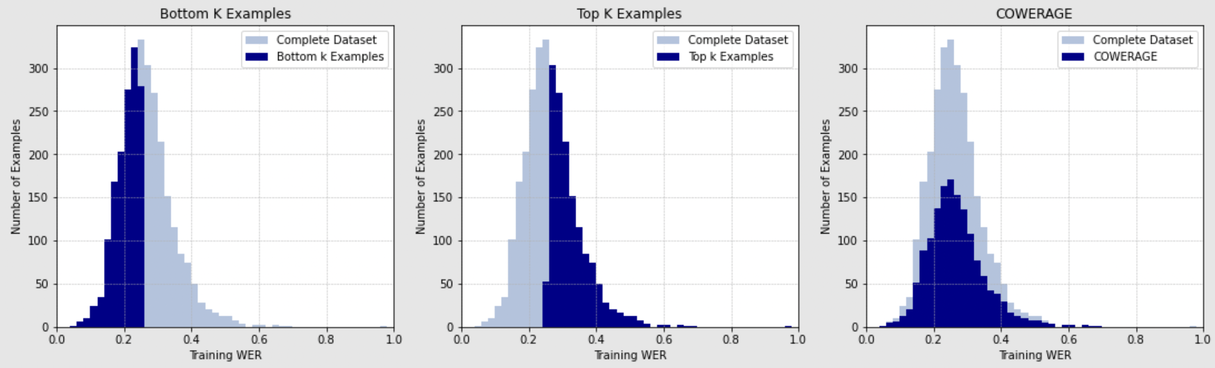
Figure 5: The subset of the Librispeech 10h training data selected by each of the three strategies: bottom k (left), top k (middle) and Cowerage (right). The pruning fraction is set to 0.5 and the WER selection epoch is 8.

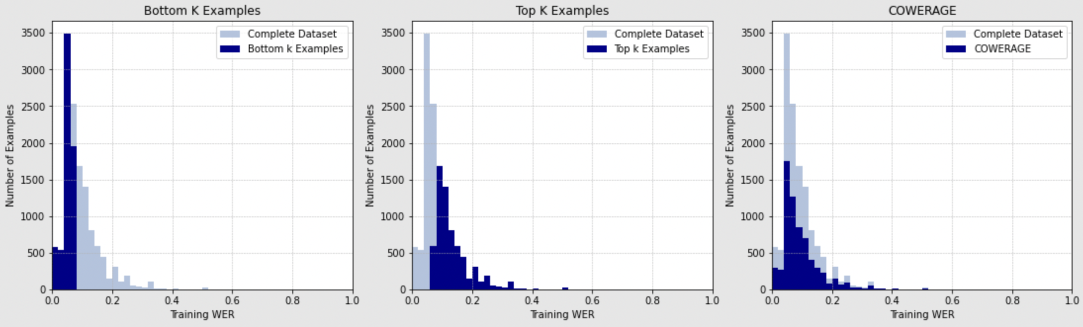
Figure 6: The subset of the LJspeech 24h training data selected by each of the three strategies: bottom k (left), top k (middle) and Cowerage (right). The pruning fraction is set to 0.5 and the WER selection epoch is 8.

B.3 Training Landscape

We now compare the training landscape for the three strategies discussed. We create four subsets of data at the pruning fraction of 0.7 and plot the training WER for each of the four approaches (Fig. 7). By examining the outlier behavior and the width of the box plots (25th to 75th percentile), we find that Cowerage subset selection is actually picking the moderately hard and representative examples instead of just the very hard but rare examples.

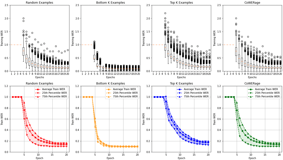
Figure 7: The training trajectories of the examples in TIMIT selected by picking the random examples (first column), bottom k examples (second column), top k examples (third column), and via Cowerage subset selection (fourth column). For each epoch, we show the box plot of the distribution of the word error rate of training examples that indicates the mean, quartiles, and outliers.

B.4 Selecting the number of buckets

We conduct an experiment with different bucket sizes on wav2vec2 and TIMIT with 0.7 pruning fraction. The results are shown in Table 7. Our evaluation shows that increasing the bucket size beyond a certain threshold provides diminishing returns in performance. Increasing the bucket size from 50 to 100 yielded 4.8% reduction in WER whereas increasing it from 100 to 500 resulted in only a 0.27% reduction in WER.

Table 7: Test WER for wav2vec2 on TIMIT for different number of buckets in the Cowerage algorithm

Number of Buckets	1	10	50	100	500	1000
Test WER	0.394	0.393	0.389	0.370	0.369	0.369

Choosing 500 buckets in the Cowerage algorithm provided robust performance across a wide range of dataset sizes, which ranged from 4620 examples in TIMIT to more than 10,000 examples in LJSpeech. The number of buckets can be increased further but it should be no greater than pruningFraction * datasetSize.

B.5 Transferability to larger models

To find out if the subsets created through a smaller model are transferable to a larger speech SSL model, we conduct an experiment with wav2vec2-large (317M parameters; pre-trained on Librispeech 960h) and fine-tune it on the subsets constructed through wav2vec2-base. We observe that Cowerage subsets still outperform the rest of the pruning strategies, further validating the hypothesis of transferability of pruning scores.

Table 8: Test WER for different for wav2vec2-large fine-tuned on subsets created through wav2vec2-base.

Strategy	Pruning Fraction
	0.1	0.3	0.5	0.7	0.9
Random	0.300	0.308	0.322	0.356	0.545
Top K	0.295	0.297	0.345	0.385	0.634
Bottom K	0.306	0.326	0.391	0.505	0.833
Cowerage	0.290	0.296	0.318	0.332	0.490

B.6 Standard deviation for test WER on TIMIT

Table 9: The standard deviation for the test WER of wav2vec2 presented in Table. 6

WSE	Strategy	Pruning Fraction
		0.1	0.3	0.5	0.7	0.9
TIMIT	Random	$\pm 0.003$	$\pm 0.005$	$\pm 0.002$	$\pm 0.025$	$\pm 0.003$
	Top K	$\pm 0.001$	$\pm 0.007$	$\pm 0.010$	$\pm 0.001$	$\pm 0.002$
	Bottom K	$\pm 0.002$	$\pm 0.002$	$\pm 0.002$	$\pm 0.009$	$\pm 0.002$
	Cowerage	$\pm 0.001$	$\pm 0.006$	$\pm 0.016$	$\pm 0.004$	$\pm 0.005$

B.7 Length and Phonemes

In this section, we examine the relationship between length and the training WER and conduct the same experiment from Section 6 but now with the length instead of the phonemic cover. The results are shown in Figure 8. The overall inverse relationship is similar to the one in Figure 3 but is noisier. We notice that there are shorter and longer sentences with a high training WER in the earlier training epochs. If we bucket the examples by length, each bucket has a higher variance of WER values than the phoneme experiment in Figure 3. We also evaluate a variant of Cowerage that selects examples on the basis of their character length instead of WER which demonstrates that WER sampling is a better subset selection strategy than length sampling for the majority of pruning fractions (Table 10).

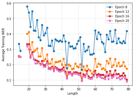
Figure 8: The training WER and the length of the examples (total number of characters) in TIMIT dataset compared over multiple training epochs. The WER is computed by averaging the training scores of the examples with the same length.

Table 10: Test WER for a variant of Cowerage that selects examples based on their length instead of WER.

Model	Strategy	Pruning Fraction
		0.1	0.3	0.5	0.7	0.9
wav2vec2-base	Cowerage (Length)	0.318	0.323	0.366	0.399	0.587
	Cowerage (WER)	0.320	0.333	0.339	0.369	0.455

B.8 Examples

Table 11: Training examples in the TIMIT dataset and their training WER on wav2vec2 along with the phonemic cover (PC). The training WER is calculated by averaging 10 runs.

WER	Text	Phonemes	PC
0.63	Twelve o’clock level.	(t-w-eh-l-v-ax-kcl-k-l-aa-kcl-k-l-eh-v-el)	10
0.63	That’s your headache.	(dh-ae-tcl-t-s-y-er-hv-eh-dx-ey-kcl-k)	13
0.6	Run-down, iron-poor.	(r-ah-n-dcl-d-aw-n-q-ay-er-n-pcl-p-ao-r )	12
0.49	Y’all wanna walk – walk, he said.	(y-ao-l-w-ao-n-ax-w-ao-kcl-pau-w-ao-kcl-k-iy-s-eh-dcl )	13
0.46	Pansies are gluttons.	(p-ae-n-z-iy-z-er-gcl-g-l-ah-tcl-en-d-z )	13
0.43	She seemed irritated.	(sh-iy-s-ey-m-dcl-d-ih-er-tcl-t-ey-dx-ix-dcl)	13
0.42	Where’re you takin’ me?	(w-er-y-ux-tcl-t-ey-kcl-k-ix-n-m-iy)	13
0.41	They’re doin’ it now.	(dh-eh-r-dcl-d-uw-ih-nx-ih-tcl-n-aw)	11
0.40	Yes, ma’am, it sure was.	(y-eh-s-epi-m-ae-m-ih-tcl-t-sh-er-w-ah-s)	13
0.40	Twenty-two or twenty-three.	(t-w-eh-n-tcl-t-iy-tcl-t-ux-ao-r-tcl-t-w-eh-n-tcl-t-iy-th-r-iy)	10
0.07	Boys and men go along the riverbank or to the alcoves in the top arcade.	(b-oy-z-ix-n-m-eh-n-gcl-g-ow-ax-l-ao-ng-n-ix-r-ih-v-er-bcl-b-ae-ng-kcl-k-q-ao-r-tcl-t-ux-dcl-d-iy-q-ae-l-kcl-k-ow-v-z-q-ix-n-dh-ix-tcl-t-aa-pcl-p-aa-r-kcl-k-ey-dcl-d)	34
0.07	But if she wasn’t interested, she’d just go back to the same life she’d left.	(b-uh-dx-ih-f-sh-iy-w-ah-z-ix-n-ih-n-tcl-t-axr-s-tcl-t-ih-dcl-d-pau-sh-iy-dcl-jh-uh-s-gcl-g-ow-bcl-b-ae-kcl-t-ix-dh-ix-s-ey-m-l-ay-f-sh-iy-dcl-l-eh-f-tcl-t)	32
0.07	Why the hell didn’t you come out when you saw them gang up on me?	(w-ay-dh-eh-hv-eh-l-dcl-d-ih-dcl-en-tcl-ch-ux-kcl-k-ah-m-aw-q-w-ix-n-y-ux-s-ao-dh-ix-m-gcl-g-ae-ng-ah-pcl-p-ao-n-m-iy)	31
0.06	You think somebody is going to stand up in the audience and make guilty faces?	(y-ux-th-ih-ng-kcl-k-s-ah-m-bcl-b-aa-dx-iy-ix-z-gcl-g-oy-ng-dcl-d-ix-s-tcl-t-ae-n-dcl-d-ah-pcl-p-ix-n-ah-q-aa-dx-iy-eh-n-tcl-s-eh-m-ey-kcl-g-ih-l-tcl-t-ix-f-ey-s-eh-z)	33
0.06	How much and how many profits could a majority take out of the losses of a few?	(hh-aw-m-ah-tcl-ch-ix-n-hv-aw-m-ax-nx-iy-pcl-p-r-aa-f-ax-tcl-s-kcl-k-uh-dx-ax-m-ax-dcl-jh-ao-axr-dx-iy-tcl-t-ey-kcl-k-ae-dx-ah-dh-ax-l-ao-s-ix-z-ax-v-ax-f-y-ux)	35
0.06	He may not rise to the heights, but he can get by, and eventually be retired.	(hh-iy-m-ey-n-aa-q-r-ay-z-tcl-t-ix-dh-ax-hv-ay-tcl-s-pau-b-ah-dx-iy-kcl-k-ix-ng-gcl-g-eh-q-bcl-b-ay-pau-q-ix-nx-iy-v-eh-n-ch-ix-l-iy-pau-b-iy-r-iy-tcl-t-ay-axr-dcl-d)	35
0.06	My sincere wish is that he continues to add to this record he sets here today.	(m-ay-s-en-s-ih-r-w-ih-sh-ix-z-dh-eh-tcl-hv-iy-kcl-k-ax-h-tcl-t-ih-n-y-ux-z-tcl-t-ax-h-q-ae-dcl-d-pau-t-ux-dh-ih-sh-r-eh-kcl-k-axr-dx-iy-s-eh-tcl-s-hh-ix-r-tcl-t-ax-h-dx-ey)	31
0.05	Then he fled, not waiting to see if she minded him or took notice of his cry.	(dh-ih-n-iy-f-l-eh-dcl-d-pau-n-aa-q-w-ey-dx-ih-ng-dcl-d-ix-s-iy-ih-f-sh-iy-m-ay-n-ix-dcl-d-hv-ih-m-pau-q-axr-tcl-t-uh-kcl-n-ow-dx-ih-s-ix-v-ix-z-kcl-k-r-ay)	32
0.01	We apply auditory modeling to computer speech recognition.	(w-iy-ax-pcl-p-l-ay-q-ao-dx-ix-tcl-t-ao-r-ix-m-aa-dx-el-ix-ng-tcl-t-uw-kcl-k-ax-m-pcl-p-y-ux-dx-er-s-pcl-p-iy-tcl-ch-epi-r-eh-kcl-k-ix-gcl-n-ih-sh-ix-n)	35

References

- Agarwal et al. (2020) Agarwal, C., D’souza, D., and Hooker, S. Estimating example difficulty using variance of gradients. arXiv preprint arXiv:2008.11600, 2020.
- Ahmed & Wahed (2020) Ahmed, N. and Wahed, M. The de-democratization of ai: Deep learning and the compute divide in artificial intelligence research. arXiv preprint arXiv:2010.15581, 2020.
- Awasthi et al. (2021) Awasthi, A., Kansal, A., Sarawagi, S., and Jyothi, P. Error-driven fixed-budget asr personalization for accented speakers. In ICASSP 2021-2021 IEEE International Conference on Acoustics, Speech and Signal Processing (ICASSP), pp. 7033–7037. IEEE, 2021.
- Azeemi et al. (2022) Azeemi, A. H., Qazi, I. A., and Raza, A. A. Dataset pruning for resource-constrained spoofed audio detection. Proc. Interspeech 2022, pp. 416–420, 2022.
- Baevski et al. (2020) Baevski, A., Zhou, H., Mohamed, A., and Auli, M. wav2vec 2.0: A framework for self-supervised learning of speech representations. arXiv preprint arXiv:2006.11477, 2020.
- Baldock et al. (2021) Baldock, R. J., Maennel, H., and Neyshabur, B. Deep learning through the lens of example difficulty. arXiv preprint arXiv:2106.09647, 2021.
- Billington et al. (2021) Billington, R., Stoakes, H., and Thieberger, N. The Pacific Expansion: Optimizing Phonetic Transcription of Archival Corpora. In Proc. Interspeech 2021, pp. 4029–4033, 2021. doi: 10.21437/Interspeech.2021-2167.
- Coleman et al. (2019) Coleman, C., Yeh, C., Mussmann, S., Mirzasoleiman, B., Bailis, P., Liang, P., Leskovec, J., and Zaharia, M. Selection via proxy: Efficient data selection for deep learning. arXiv preprint arXiv:1906.11829, 2019.
- Dong et al. (2019) Dong, L., Guo, Q., and Wu, W. Speech corpora subset selection based on time-continuous utterances features. Journal of Combinatorial Optimization, 37(4):1237–1248, 2019.
- Durga et al. (2021) Durga, S., Iyer, R., Ramakrishnan, G., and De, A. Training data subset selection for regression with controlled generalization error. In International Conference on Machine Learning, pp. 9202–9212. PMLR, 2021.
- Garofolo et al. (1993) Garofolo, J. S., Lamel, L. F., Fisher, W. M., Fiscus, J. G., and Pallett, D. S. Darpa timit acoustic-phonetic continous speech corpus cd-rom. nist speech disc 1-1.1. NASA STI/Recon technical report n, 93:27403, 1993.
- Graves et al. (2006) Graves, A., Fernández, S., Gomez, F., and Schmidhuber, J. Connectionist temporal classification: labelling unsegmented sequence data with recurrent neural networks. In Proceedings of the 23rd international conference on Machine learning, pp. 369–376, 2006.
- Han et al. (2011) Han, J., Pei, J., and Kamber, M. Data mining: concepts and techniques. Elsevier, 2011.
- Hsu et al. (2021) Hsu, W.-N., Bolte, B., Tsai, Y.-H. H., Lakhotia, K., Salakhutdinov, R., and Mohamed, A. Hubert: Self-supervised speech representation learning by masked prediction of hidden units. arXiv preprint arXiv:2106.07447, 2021.
- Huang et al. (2021) Huang, L., Sudhir, K., and Vishnoi, N. Coresets for time series clustering. Advances in Neural Information Processing Systems, 34, 2021.
- Ito & Johnson (2017) Ito, K. and Johnson, L. The lj speech dataset, 2017.
- Jiang et al. (2021) Jiang, S., Krauthgamer, R., Wu, X., et al. Coresets for clustering with missing values. Advances in Neural Information Processing Systems, 34, 2021.
- Jubran et al. (2021) Jubran, I., Sanches Shayda, E. E., Newman, I., and Feldman, D. Coresets for decision trees of signals. Advances in Neural Information Processing Systems, 34, 2021.
- Karamcheti et al. (2021) Karamcheti, S., Krishna, R., Fei-Fei, L., and Manning, C. D. Mind your outliers! investigating the negative impact of outliers on active learning for visual question answering. arXiv preprint arXiv:2107.02331, 2021.
- Killamsetty et al. (2021) Killamsetty, K., Sivasubramanian, D., Mirzasoleiman, B., Ramakrishnan, G., De, A., and Iyer, R. Grad-match: A gradient matching based data subset selection for efficient learning. arXiv preprint arXiv:2103.00123, 2021.
- Kothawade et al. (2021) Kothawade, S., Beck, N., Killamsetty, K., and Iyer, R. Similar: Submodular information measures based active learning in realistic scenarios. Advances in Neural Information Processing Systems, 34, 2021.
- Kothyari et al. (2021) Kothyari, M., Mekala, A. R., Iyer, R., Ramakrishnan, G., and Jyothi, P. Personalizing asr with limited data using targeted subset selection. arXiv preprint arXiv:2110.04908, 2021.
- Lai et al. (2021) Lai, C.-I. J., Zhang, Y., Liu, A. H., Chang, S., Liao, Y.-L., Chuang, Y.-S., Qian, K., Khurana, S., Cox, D., and Glass, J. Parp: Prune, adjust and re-prune for self-supervised speech recognition. arXiv preprint arXiv:2106.05933, 2021.
- Liu et al. (2022) Liu, A. H., Hsu, W.-N., Auli, M., and Baevski, A. Towards end-to-end unsupervised speech recognition. arXiv preprint arXiv:2204.02492, 2022.
- Margatina et al. (2021) Margatina, K., Vernikos, G., Barrault, L., and Aletras, N. Active learning by acquiring contrastive examples. In Proceedings of the 2021 Conference on Empirical Methods in Natural Language Processing, pp. 650–663, Online and Punta Cana, Dominican Republic, November 2021. Association for Computational Linguistics.
- Mendonça et al. (2014) Mendonça, G., Candeias, S., Perdigao, F., Shulby, C., Toniazzo, R., Klautau, A., and Aluísio, S. A method for the extraction of phonetically-rich triphone sentences. In 2014 International Telecommunications Symposium (ITS), pp. 1–5. IEEE, 2014.
- Mindermann et al. (2022) Mindermann, S., Brauner, J. M., Razzak, M. T., Sharma, M., Kirsch, A., Xu, W., Höltgen, B., Gomez, A. N., Morisot, A., Farquhar, S., et al. Prioritized training on points that are learnable, worth learning, and not yet learnt. In International Conference on Machine Learning, pp. 15630–15649. PMLR, 2022.
- Mirzasoleiman et al. (2020) Mirzasoleiman, B., Bilmes, J., and Leskovec, J. Coresets for data-efficient training of machine learning models. In International Conference on Machine Learning, pp. 6950–6960. PMLR, 2020.
- Ni et al. (2015a) Ni, C., Leung, C.-C., Wang, L., Chen, N. F., and Ma, B. Unsupervised data selection and word-morph mixed language model for tamil low-resource keyword search. In 2015 IEEE International Conference on Acoustics, Speech and Signal Processing (ICASSP), pp. 4714–4718. IEEE, 2015a.
- Ni et al. (2015b) Ni, C., Wang, L., Liu, H., Leung, C.-C., Lu, L., and Ma, B. Submodular data selection with acoustic and phonetic features for automatic speech recognition. In 2015 IEEE International Conference on Acoustics, Speech and Signal Processing (ICASSP), pp. 4629–4633. IEEE, 2015b.
- Ni et al. (2016) Ni, C., Leung, C.-C., Wang, L., Liu, H., Rao, F., Lu, L., Chen, N. F., Ma, B., and Li, H. Cross-lingual deep neural network based submodular unbiased data selection for low-resource keyword search. In 2016 IEEE International Conference on Acoustics, Speech and Signal Processing (ICASSP), pp. 6015–6019. IEEE, 2016.
- Panayotov et al. (2015) Panayotov, V., Chen, G., Povey, D., and Khudanpur, S. Librispeech: an asr corpus based on public domain audio books. In 2015 IEEE international conference on acoustics, speech and signal processing (ICASSP), pp. 5206–5210. IEEE, 2015.
- Paul et al. (2021) Paul, M., Ganguli, S., and Dziugaite, G. K. Deep learning on a data diet: Finding important examples early in training. Advances in Neural Information Processing Systems, 34, 2021.
- Raju et al. (2021) Raju, R. S., Daruwalla, K., and Lipasti, M. Accelerating deep learning with dynamic data pruning. arXiv preprint arXiv:2111.12621, 2021.
- Schirrmeister et al. (2022) Schirrmeister, R. T., Liu, R., Hooker, S., and Ball, T. When less is more: Simplifying inputs aids neural network understanding. arXiv preprint arXiv:2201.05610, 2022.
- Shim et al. (2021) Shim, K., Choi, J., and Sung, W. Understanding the role of self attention for efficient speech recognition. In International Conference on Learning Representations, 2021.
- Sorscher et al. (2022) Sorscher, B., Geirhos, R., Shekhar, S., Ganguli, S., and Morcos, A. S. Beyond neural scaling laws: beating power law scaling via data pruning. arXiv preprint arXiv:2206.14486, 2022.
- Thomas et al. (2022) Thomas, B., Kessler, S., and Karout, S. Efficient adapter transfer of self-supervised speech models for automatic speech recognition. In ICASSP 2022-2022 IEEE International Conference on Acoustics, Speech and Signal Processing (ICASSP), pp. 7102–7106. IEEE, 2022.
- Tolochinsky & Feldman (2018) Tolochinsky, E. and Feldman, D. Coresets for monotonic functions with applications to deep learning. CoRR, abs/1802.07382, 2018.
- Toneva et al. (2018) Toneva, M., Sordoni, A., Combes, R. T. d., Trischler, A., Bengio, Y., and Gordon, G. J. An empirical study of example forgetting during deep neural network learning. arXiv preprint arXiv:1812.05159, 2018.
- Wei et al. (2014) Wei, K., Liu, Y., Kirchhoff, K., Bartels, C., and Bilmes, J. Submodular subset selection for large-scale speech training data. In 2014 IEEE International Conference on Acoustics, Speech and Signal Processing (ICASSP), pp. 3311–3315. IEEE, 2014.
- Wolf et al. (2019) Wolf, T., Debut, L., Sanh, V., Chaumond, J., Delangue, C., Moi, A., Cistac, P., Rault, T., Louf, R., Funtowicz, M., et al. Huggingface’s transformers: State-of-the-art natural language processing. arXiv preprint arXiv:1910.03771, 2019.
- Woodard & Nelson (1982) Woodard, J. and Nelson, J. An information theoretic measure of speech recognition performance. In Workshop on standardisation for speech I/O technology, Naval Air Development Center, Warminster, PA, 1982.
- Wu et al. (2007) Wu, Y., Zhang, R., and Rudnicky, A. Data selection for speech recognition. In 2007 IEEE Workshop on Automatic Speech Recognition & Understanding (ASRU), pp. 562–565. IEEE, 2007.
- Wu et al. (2021) Wu, Z., Zhao, D., Liang, Q., Yu, J., Gulati, A., and Pang, R. Dynamic sparsity neural networks for automatic speech recognition. In ICASSP 2021-2021 IEEE International Conference on Acoustics, Speech and Signal Processing (ICASSP), pp. 6014–6018. IEEE, 2021.
- Zhen et al. (2021) Zhen, K., Nguyen, H. D., Chang, F.-J., Mouchtaris, A., and Rastrow, A. Sparsification via compressed sensing for automatic speech recognition. In ICASSP 2021-2021 IEEE International Conference on Acoustics, Speech and Signal Processing (ICASSP), pp. 6009–6013. IEEE, 2021.