Probing Three-Dimensional Magnetic Fields: I - Polarized Dust Emission

Abstract

Polarized dust emission is widely used to trace the plane-of-the-sky (POS) component of interstellar magnetic fields in two dimensions. Its potential to access three-dimensional magnetic fields, including the inclination angle of the magnetic fields relative to the line-of-sight (LOS), is crucial for a variety of astrophysical problems. Based on the statistical features of observed polarization fraction and POS Alfvén Mach number $\overline{M_{\rm A}}_{,\bot}$ distribution, we present a new method for estimating the inclination angle. The magnetic field fluctuations raised by anisotropic magnetohydrodynamic (MHD) turbulence are taken into account in our method. By using synthetic dust emission generated from 3D compressible MHD turbulence simulations, we show that the fluctuations are preferentially perpendicular to the mean magnetic field. We find the inclination angle is the major agent for depolarization, while fluctuations of magnetic field strength and density have an insignificant contribution. We propose and demonstrate that the mean inclination angle over a region of interest can be calculated from the polarization fraction in a strongly magnetized reference position, where $\overline{M_{\rm A}}_{,\bot}^{2}\ll 1$. We test and show that the new method can trace the 3D magnetic fields in sub-Alfvénic, trans-Alfvénic, and moderately super-Alfvénic conditions ($0.4\lesssim M_{\rm A}\lesssim 1.2$). We numerically quantify that the difference of the estimated inclination angle and actual inclination angle ranges from 0 to $20^{\circ}$ with a median value of $\leq 10^{\circ}$.

1 Introduction

In interstellar medium (ISM), magnetic field is one of the most important components (Ruzmaikin et al., 1988; Planck Collaboration et al., 2016a, b; Han, 2017; Clark & Hensley, 2019; Hu et al., 2020a, 2022a). It is crucial in balancing the ISM with gravity (Myers & Goodman, 1988; Allen et al., 2003; Wurster & Li, 2018; Abbate et al., 2020), regulating turbulent gas flows (Uchida & Shibata, 1985; Roche et al., 2018; Busquet, 2020), and constraining cosmic ray’s transport (Jokipii, 1966; Ghilea et al., 2011; Xu & Yan, 2013; Hu et al., 2022b; Beattie et al., 2022). In particular, magnetic field is a key factor influencing the dynamics of the star-forming process in molecular clouds (Mac Low & Klessen, 2004; Crutcher, 2004; McKee & Ostriker, 2007; Lazarian et al., 2012; Crutcher, 2012; Federrath & Klessen, 2012; Hu et al., 2021b). In view of its importance, a number of ways to access the magnetic field have been proposed. For instance, polarized dust emission (Lazarian, 2007; Andersson et al., 2015; Planck Collaboration et al., 2015a, 2020; Fissel et al., 2016; Li et al., 2021) and synchrotron emission (Xiao et al., 2008; Planck Collaboration et al., 2016c; Guan et al., 2021) can trace the POS magnetic field, while Zeenman splitting (Crutcher, 2004, 2012) and Faraday rotation (Haverkorn, 2007; Taylor et al., 2009; Oppermann et al., 2012; Xu & Zhang, 2016) reveal the LOS magnetic field strength. However, because they probe different regions of the multi-phase ISM, the measurements cannot easily be combined to yield full 3D magnetic field vectors. Probing a three-dimensional magnetic field that includes both the POS and the LOS components simultaneously remains a challenge.

Intense attempts have been undertaken to get the 3D magnetic field at cloud scales. For instance, Lazarian & Yuen (2018b) proposed a solution using the wavelength derivative of synchrotron polarization. Tahani et al. (2019); Tahani et al. (2022) used the changed sign of LOS magnetic fields obtained by Tahani et al. (2018) to infer bow-shaped magnetic field morphologies across the Orion-A and Perseus molecular clouds. Zhang et al. (2020) achieved a three-dimensional magnetic field via the fraction and direction of atomic gas’s polarization. After that, Hu et al. (2021a) suggested using MHD turbulence’s anisotropic property inherited by young stellar objects to obtain a three-dimensional view of the magnetic field. Similarly, based on anisotropic MHD turbulence, Hu et al. (2021c) further extend the method to be applicable for Doppler-shifted emission lines in three-dimension. The LOS and POS components of the magnetic field’s orientation and strength can be calculated simultaneously for the latter two methods.

In addition to the approaches mentioned above, an important step of probing the 3D magnetic field via polarized dust emission was initiated by Chen et al. (2019). The POS magnetic field can be easily inferred from polarization direction based on the fact that dust grains preferentially align with their ambient magnetic fields (Lazarian, 2007; Andersson et al., 2015). To achieve a three-dimensional picture, the inclination angle of the magnetic field relative to the LOS is crucial. As the inclination angle is one of the major agents of depolarizing thermal emission from dust, the polarization fraction intrinsically inherits the angle’s information. Therefore, Chen et al. (2019) and Sullivan et al. (2021) estimated the inclination angle based on the statistical properties of the observed polarization fraction. Their method assumes an ideal scenario that there are no fluctuations in neither magnetic field’s POS nor LOS components. This assumption could be valid for strongly magnetized mediums. However, molecular clouds are typically trans-Alfvénic or even super-Alfvénic (Federrath et al., 2016; Hu et al., 2019; Hwang et al., 2021; Li et al., 2021), in which the fluctuations are not negligible.

To accommodate the magnetic field fluctuations, here we consider a scenario that the fluctuations arise from anisotropic magnetohydrodynamic (MHD) turbulence based on the fact that molecular cloud is highly turbulent (Larson, 1981; Myers, 1983; Evans, 1999; Hennebelle & Falgarone, 2012) and is dominated by slow and fast components of MHD turbulence that follow Kolmogorov scaling (Yuen et al., 2022). This consideration advantageously simplifies the problem because the most significant fluctuations preferentially appear in the direction perpendicular to the mean magnetic field (Goldreich & Sridhar, 1995; Lazarian & Vishniac, 1999; Cho & Lazarian, 2003). Therefore, we propose a simple model in this work that the local magnetic field along the LOS is built up by a global mean magnetic field and perpendicular fluctuations. This assumption is typically valid for cloud-scale and clump-scale objects in which their magnetic fields’ variation along the LOS is insignificant.

By incorporating the magnetic field fluctuations, this work aims at developing a method to probe the 3D magnetic field in sub-, trans- and super-Alfvénic clouds. This method requires the knowledge of the polarization fraction and the POS Alfvén Mach number’s distributions. The latter can be obtained by a number of approaches. To test the proposed method, we use 3D MHD turbulence simulations to generate synthetic dust emissions. We will show that the assumption of perpendicular fluctuations is also valid in the presence of compressible turbulence.

This paper is organized as follows. We briefly review the basic concepts of MHD turbulence and show the derivation of how to estimate the magnetic field’s inclination angle from polarized dust emission. In § 3, we give the details of the simulation’s setup and numerical method. We applied our method to the simulations in § 4 and made a comparison with the method proposed in Chen et al. (2019). In § 5, we discuss the systematic uncertainties raised by our assumptions and list several approaches to getting the POS Alfvén Mach number’s distribution. We summarize our results in § 6.

2 Theoretical consideration

2.1 Essential elements of MHD turbulence

Our understanding of MHD turbulence has been significantly changed in the past decades. MHD turbulence was initially considered to be isotropic despite the existence of magnetic fields (Iroshnikov, 1963; Kraichnan, 1965). However, a number of numerical studies (Montgomery & Turner, 1981; Shebalin et al., 1983; Higdon, 1984; Kraichnan, 1965; Montgomery & Matthaeus, 1995; Maron & Goldreich, 2001; Kowal & Lazarian, 2010; Hu et al., 2021c) and in situ measurements of solar wind (Wang et al., 2016) revealed that the turbulence is anisotropic rather than isotropic when magnetic field’s role is not negligible.

A fundamental work on the anisotropic incompressible MHD turbulence theory was done by Goldreich & Sridhar (1995) for the trans-Alfvénic regime, i.e. for injection velocity equal to the Alfvén velocity and was extended to sub-Alfvénic turbulence, i.e. for injection velocity less than the Alfven velocity (Lazarian & Vishniac, 1999).

The modern picture of MHD turbulence cascade states that the Alfvénic mode cascade is channeled to the field’s perpendicular direction. This is achievable because turbulent reconnection, as an intrinsic part of the MHD turbulent cascade, happens over one eddy turnover time and enables the mixing of magnetic field lines perpendicular to the magnetic field direction (Lazarian & Vishniac, 1999). Thus mixing presents the path of minimal resistance for turbulent motions and the turbulence is channeled along this path. More detail is available in Beresnyak & Lazarian (2019), where the properties of compressible MHD turbulence are described in detail.

The fluctuations of turbulent velocity therefore is preferentially along the perpendicular direction. From the scaling of MHD turbulence in (Lazarian & Vishniac, 1999) it follows that the ratio of squared velocity fluctuations at scale $l$ along the perpendicular (i.e., $v_{l,\bot}^{2}$) and the parallel directions (i.e., $v_{l,\parallel}^{2}$) with respect to the local magnetic field is (Hu et al., 2021a):

$$v_{l,\bot}^{2}/v_{l,\parallel}^{2}=(l_{\parallel}/L_{\rm inj})^{-1/3}M_{\rm A}^{-4/3},$$ (1)

here $M_{\rm A}$ is the Alfvén Mach number and $L_{\rm inj}$ is the injection scale of turbulence. $l_{\parallel}$ denotes the scale parallel to the local magnetic field, i.e., the magnetic field passing through the turbulent eddy. The injection scale $L_{\rm inj}$ is approximately 100 pc in our galaxy (Armstrong et al., 1995; Chepurnov & Lazarian, 2010; Yuen et al., 2022) and is much greater than the scale $\ll 0.1$ pc that can be resolved in observation (Chuss et al., 2019; Zielinski & Wolf, 2022; Fanciullo et al., 2022). The velocity fluctuations raised from incompressible MHD turbulence are therefore dominantly along the magnetic field’s perpendicular direction for our consideration of molecular clouds and even smaller clumps.

From the induction equation, one can easily find that the magnetic field fluctuation at scale $l$ is perpendicular to the plane spanned by the global mean magnetic field $\langle\boldsymbol{B}\rangle$ and displacement vector $\boldsymbol{\hat{\xi}}$ of plasma in incompressible turbulence (Cho & Lazarian, 2003):

$$\delta\boldsymbol{B}_{l,\bot}=\frac{v_{l,\bot}}{v_{\rm A}}({\langle\boldsymbol{B}\rangle}\times\boldsymbol{\hat{\xi}}),$$ (2)

where $v_{\rm A}$ is the Alfvén speed. In polarization studies, the statistical description of such fluctuations was provided in Lazarian & Pogosyan (2012). This agrees well with the numerical studies of compressible MHD turbulence in Hu et al. (2021a). A more detailed discussion of magnetic fluctuations in compressible turbulence is given in § 5.

2.2 Estimating inclination angle from dust polarization

Based on the fact that we in polarization measurements we deal with magnetic field fluctuation preferentially perpendicular to the mean field, we can investigate the properties of polarized dust emission.

We adopt dust polarization equations from Planck Collaboration et al. (2015b):

$$I(x,y) =\int n[1-p_{0}(\sin^{2}\gamma-2/3)]dz,$$ (3)

$$Q(x,y) =\int p_{0}n\frac{B_{x}^{2}-B_{y}^{2}}{B^{2}}dz,$$

$$U(x,y) =\int p_{0}n\frac{2B_{x}B_{y}}{B^{2}}dz,$$

$$\psi(x,y) =\frac{1}{2}\tan^{-1}(\frac{U}{Q}),$$

where $n(x,y,z)$ is dust volume density, $\psi$ is polarization angle, and $p_{0}$ is a polarization fraction parameter related to the intrinsic polarization fraction (assumed to be constant throughout a cloud; Chen et al. 2019). $B(x,y,z)$ denotes total magnetic field strength, while $B_{x}(x,y,z)$ and $B_{y}(x,y,z)$ are its x-axis component and $y$-axis component. $\gamma$ is the magnetic field’s inclination angle with respect to the LOS (i.e., the $z$-axis). Accordingly, the polarization fraction is (Fiege & Pudritz, 2000):

$$p=\frac{\sqrt{Q^{2}+U^{2}}}{I}=p_{0}\frac{\sqrt{(\int n\frac{B_{x}^{2}-B_{y}^{2}}{B^{2}}dz)^{2}+(\int n\frac{2B_{x}B_{y}}{B^{2}}dz)^{2}}}{\int ndz-p_{0}\int n(\sin^{2}\gamma-2/3)dz}.$$ (4)

Figure 1: Illustration of the magnetic field configuration. Panel a: configuration of the mean field $\langle\boldsymbol{B}\rangle$. $\langle\boldsymbol{B}\rangle_{\bot}$ is the magnetic field projected on the POS, i.e. $xy$ plane. $\langle\gamma\rangle$ is the mean inclination angle of the mean magnetic field $\langle\boldsymbol{B}\rangle$ with respect to the LOS. $\langle\phi\rangle=\langle\psi\rangle+\pi/2$ is the magnetic field’s angle relative to $x$-axis on the POS. Panel b: configuration of the local total magnetic field $\boldsymbol{B}=\langle\boldsymbol{B}\rangle+\delta\boldsymbol{B}$. The mean field is changed by a perpendicular fluctuation $\delta\boldsymbol{B}$ with an angle $\theta$. Here $\theta$ is the angle between $\delta\boldsymbol{B}$ and the vector (i.e., $\delta\boldsymbol{B}\sin\theta$) that is simultaneously perpendicular to $\langle\boldsymbol{B}\rangle$ and $\hat{\langle\boldsymbol{B}\rangle}\times\hat{\boldsymbol{z}}$. Dashed black lines are within the $\hat{\langle\boldsymbol{B}\rangle}-\hat{\boldsymbol{z}}$ plane, where $\hat{\langle\boldsymbol{B}\rangle}$ and $\hat{z}$ are unit vectors of $\langle\boldsymbol{B}\rangle$ and $\boldsymbol{z}$, respectively.

To describe magnetic field fluctuations, we use a simple configuration of magnetic field (see Fig. 1). Assuming the local total magnetic field is built up by a mean magnetic field $\langle\boldsymbol{B}\rangle$ and a fluctuation $\delta\boldsymbol{B}(x,y,z)$:

$$\boldsymbol{B}(x,y,z)=\langle\boldsymbol{B}\rangle+\delta\boldsymbol{B}(x,y,z),$$ (5)

The mean-field also has a mean inclination angle $\langle\gamma\rangle$ and POS magnetic field angle $\langle\phi\rangle$. We consider the magnetic field fluctuation $\delta\boldsymbol{B}$ that is preferentially perpendicular to the mean field. However, since $\delta\boldsymbol{B}\propto\hat{\boldsymbol{\xi}}\times\langle\boldsymbol{B}\rangle$, the fluctuation does not necessarily lie on the plane defined by $\langle\boldsymbol{B}\rangle$ and the LOS (i.e., the $z$-axis). Instead, we consider that $\delta\boldsymbol{B}$ has an angle $\theta$ with respect to the $\langle\boldsymbol{B}\rangle-z$ plane. Specifically, $\theta$ is that angle between $\delta\boldsymbol{B}$ and the vector that is simultaneously perpendicular to $\langle\boldsymbol{B}\rangle$ and $\hat{\langle\boldsymbol{B}\rangle}\times\hat{z}$ (see Fig. 1). Accordingly, we project the fluctuations and mean field into $x$ and $y$ components:

$$B_{x} =\langle B\rangle\sin\langle\gamma\rangle\cos\langle\phi\rangle+(\delta B\cos\theta)\cos\langle\gamma\rangle\cos\langle\phi\rangle-(\delta B\sin\theta)\sin\langle\phi\rangle,$$ (6)

$$B_{y} =\langle B\rangle\sin\langle\gamma\rangle\sin\langle\phi\rangle+(\delta B\cos\theta)\cos\langle\gamma\rangle\sin\langle\phi\rangle+(\delta B\sin\theta)\cos\langle\phi\rangle.$$

The first term comes from the mean magnetic field angle $\langle\phi\rangle$ and mean inclination angle $\langle\gamma\rangle$. Their fluctuations $\delta\gamma$ and $\delta\phi$ are introduced by the last two terms involved with $\delta\boldsymbol{B}$.

Note that the direction of $\delta\boldsymbol{B}$ is defined by the displacement vector and the mean field (see Eq. 2). As the displacement vector varies in different spatial positions along the LOS, $\theta$ is not a constant. By assuming a uniform distribution of $\theta$ along the LOS, we integrate $\theta$ from 0 to $2\pi$ and take averages:

$$Q =\frac{1}{2\pi}\int p_{0}n\int_{0}^{2\pi}\frac{B_{x}^{2}-B_{y}^{2}}{B^{2}}d\theta dz$$ (7)

$$=\int p_{0}n\frac{\cos(2\langle\psi\rangle)[\sin^{2}\langle\gamma\rangle+\frac{1}{2}M_{\rm A}^{2}\cos^{2}\langle\gamma\rangle-\frac{1}{2}M_{\rm A}^{2}]}{1+M_{\rm A}^{2}}dz,$$

$$U =\frac{1}{2\pi}\int p_{0}n\int_{0}^{2\pi}\frac{2B_{x}B_{y}}{B^{2}}d\theta dz$$

$$=\int p_{0}n\frac{\sin(2\langle\psi\rangle)[\sin^{2}\langle\gamma\rangle+\frac{1}{2}M_{\rm A}^{2}\cos^{2}\langle\gamma\rangle-\frac{1}{2}M_{\rm A}^{2}]}{1+M_{\rm A}^{2}}dz,$$

$$\frac{1}{2\pi} \int_{0}^{2\pi}\sin^{2}\gamma d\theta=\frac{1}{2\pi}\int_{0}^{2\pi}(1-\cos^{2}\gamma)d\theta$$

$$=1-\frac{M_{\rm A}^{2}\sin^{2}\langle\gamma\rangle}{2(M_{\rm A}^{2}+1)}-\frac{\cos^{2}\langle\gamma\rangle}{M_{\rm A}^{2}+1}.$$

Eq. 7 gives the effective values of the three quantities along single LOS. Here $M_{\rm A}=\delta B/\langle B\rangle$ is the Alfvén Mach number..

In the presence of a mean magnetic field, the integral of local $M_{\rm A}$ weighted by density $n$ can be replaced with its mean value $\overline{M_{\rm A}}$ averaged along the LOS, as a first order approximation. In this work, upper "$-$" symbol means LOS average, while $\langle...\rangle$ is averaged over a volume of interest.

For convenience, we introduce $\overline{M}_{\rm A,\bot}$, which is the Alfvén Mach number corresponding to the motions perpendicular to the LOS, i.e.:

$${\overline{M}_{\rm A,\bot}} =(v_{l}\sqrt{4\pi{\overline{\rho}}})/(\langle B\rangle\sin{\overline{\gamma}})=v_{l}/({\overline{v}_{A}}\sin{\overline{\gamma}})$$ (8)

$$={\overline{M}_{\rm A}}/\sin{\overline{\gamma}},$$

where ${\overline{\rho}}$ is mean gas mass density. The 3D turbulent velocity $v_{l}$ has been already incorporated in available observational methods (see § 5) of calculating $\overline{M}_{\rm A,\bot}$. For instance, the Davis-Chandrasekhar-Fermi (DCF) method (Davis, 1951; Chandrasekhar & Fermi, 1953) calculates $v_{l}$ from the emission line’s width (Hwang et al., 2021) . The projection, therefore, is applied only to the total magnetic field strength.

Combining Eqs. 4 and 7, the polarization fraction can be written as:

$$p =\frac{p_{0}}{1+\overline{M_{\rm A}}^{2}}\cdot\frac{\sin^{2}\langle\gamma\rangle(1-\frac{1}{2}\overline{M_{\rm A}}^{2})}{1-p_{0}(1/3-\frac{\sin^{2}\langle\gamma\rangle(\overline{M_{\rm A}}^{2}-2)+2}{2(\overline{M_{\rm A}}^{2}+1)})}.$$ (9)

Note here we write the Eq. 4’s integral of the product in the numerators’ two terms and the denominator second term as a product of two integrals (one is $\int ndz$) as we disregard the correlation of fluctuations of density and magnetic field. Consequently, the column density $\int ndz$ appears in both numerator and denominator and is cancelled off. In reality, the observationally measured polarization angle and inclination angle are density weighted. However, the main effect for polarization is expected from the variations of the magnetic field direction.

As shown in Fig. 2, the variations of the magnetic field direction along the LOS induce depolarization effects so that $p$ get its minimum value at large $\overline{M_{\rm A}}$. In observations, as $p$ is measured, the key problem in determining $\sin^{2}\langle\gamma\rangle$ is to get $p_{0}$ and $\overline{M_{\rm A}}$. Chen et al. (2019) showed that $p_{0}$ can be recovered approximately from:

$$p_{0}=\frac{3p_{\rm max}}{3+p_{\rm max}},$$ (10)

where $p_{\rm max}$ is the maximum polarization fraction that can be obtained when the local inclination angle is 90^∘. The discussion of uncertainties of $p_{\rm max}$ determination within our treatment is given in § 5.

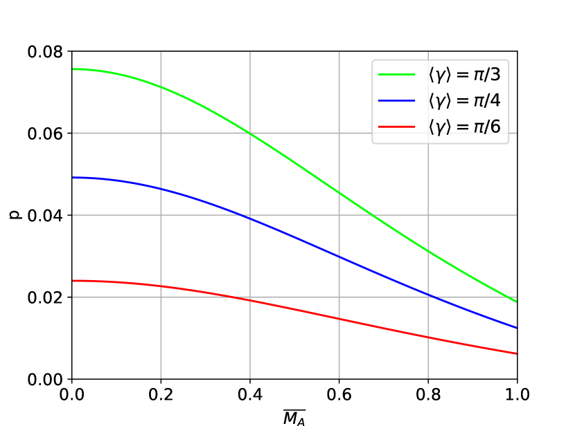
Figure 2: Analytical relation Eq. 9 of the polarization fraction $p$ and $\overline{M_{\rm A}}$.

If we know $p_{0}$, we can express the distribution of total Mach number explicitly from the observed polarization fraction $p$:

$$\overline{M_{\rm A}}^{2}=\frac{p_{0}\sin^{2}\langle\gamma\rangle(1+p)-p(1+\frac{2}{3}p_{0})}{\frac{1}{2}p_{0}\sin^{2}\langle\gamma\rangle(1+p)+p(1-\frac{1}{3}p_{0})}.$$ (11)

Note that the condition $\overline{M_{\rm A}}\geq 0$ implicitly restricts the numerator to be non-negative.

With the assumption of vanishing fluctuations ($\overline{M_{\rm A}}^{2}\approx 0$), Chen et al. (2019) generalized Eq. 11 to every LOS to get local $\overline{\gamma}$ instead of the mean value $\langle\gamma\rangle$:

$$\sin^{2}\overline{\gamma}_{\rm Ch}=\frac{p(1+\frac{2}{3}p_{0})}{p_{0}(1+p)},$$ (12)

where the subscript "$\rm Ch$" is used to distinguish the expression in Chen et al. (2019) from our expression. Here we see an inconsistency in the treatment of the problem in Chen et al. (2019). The condition $\overline{M_{\rm A}}^{2}\approx 0$ cannot be satisfied for every LOS in observation. As we are interested in the realistic situation of $\overline{M_{\rm A}}$ being nonzero, by accounting for $\overline{M_{\rm A}}$, we address this inconsistency. Combining Eq. 8 and Eq. 11, the expression for local $\sin{\overline{\gamma}}$ is:

$$\sin^{2}\overline{\gamma}=\frac{1}{\overline{M_{\rm A}}_{,\bot}^{2}}\cdot\frac{p_{0}\sin^{2}\langle\gamma\rangle(1+p)-p(1+\frac{2}{3}p_{0})}{\frac{1}{2}p_{0}\sin^{2}\langle\gamma\rangle(1+p)+p(1-\frac{1}{3}p_{0})}.$$ (13)

Or alternatively, we have:

$$p=\frac{p_{0}}{1+\overline{M_{\rm A}}_{,\bot}^{2}\sin^{2}\overline{\gamma}}\cdot\frac{\sin^{2}\langle\gamma\rangle(1-\frac{1}{2}\overline{M_{\rm A}}_{,\bot}^{2}\sin^{2}\overline{\gamma})}{1-p_{0}(1/3-\frac{\sin^{2}\langle\gamma\rangle(\overline{M_{\rm A}}_{,\bot}^{2}\sin\overline{\gamma}^{2}-2)+2}{2(\overline{M_{\rm A}}_{,\bot}^{2}\sin^{2}\overline{\gamma}+1)})}.$$ (14)

In the situation of the zeroth order approximation $\overline{M_{\rm A}}_{,\bot}^{2}\approx 0$, the contribution from $\overline{M_{\rm A}}_{,\bot}^{2}\sin^{2}\overline{\gamma}$ vanished. Or in other situation that $\overline{M_{\rm A}}_{,\bot}^{2}$ is the leading term, the condition $\overline{M_{\rm A}}_{,\bot}^{2}\ll 1$ also guarantees that $\overline{M_{\rm A}}_{,\bot}^{2}\sin^{2}\overline{\gamma}$ is negligible. Consequently, if one can find a LOS satisfying $\overline{M_{\rm A}}_{,\bot}^{2}\ll 1$, Eq. 14 reduces to:

$$p_{\rm off} =\frac{p_{0}\sin^{2}\langle\gamma\rangle_{\rm off}}{1-p_{0}(\sin^{2}\langle\gamma\rangle_{\rm off}-\frac{2}{3})},~{}~{}~{}\overline{M_{\rm A}}_{,\bot}^{2}\ll 1,$$ (15)

where $p_{\rm off}$ is the polarization fraction corresponding to $\overline{M_{\rm A}}_{,\bot}\ll 1$. Equivalently, the mean inclination angle is:

$$\sin^{2}\langle\gamma\rangle_{\rm off} =\frac{p_{\rm off}(1+\frac{2}{3}p_{0})}{p_{0}(1+p_{\rm off})},~{}~{}~{}\overline{M_{\rm A}}_{,\bot}^{2}\ll 1,$$ (16)

where the subscript "off" represents that the mean inclination angle is calculated with the knowledge of polarization fraction and $\overline{M_{\rm A}}_{,\bot}$ at a reference position. In this work, we explore the combination of Eqs. 10 and 16 in obtaining three-dimensional magnetic field assuming $\overline{M_{\rm A}}_{,\bot}^{2}$ is the leading term:

$$\sin^{2}\langle\gamma\rangle_{\rm off}=\frac{p_{\rm off}(1+p_{\rm max})}{p_{\rm max}(1+p_{\rm off})},~{}~{}~{}\overline{M_{\rm A}}_{,\bot}^{2}\ll 1.$$ (17)

Also, the total mean Alfvén Mach number can be naturally accessed via $\langle\overline{M_{\rm A}}_{,\bot}\rangle\sin\langle{\gamma}\rangle_{\rm off}=\langle\overline{M_{\rm A}}\rangle$. Note that Eq. 10 assumes that local inclination angle can achieve 90^∘, which, however, might not be the case in observation. We, therefore, generalize $p_{\max}$ to the maximum value of observed polarization fraction. Although this generalization introduces uncertainty to the estimation of $\sin^{2}\langle\gamma\rangle_{\rm off}$, we numerically find it is insignificant (see § 4).

Moreover, Eq. 17 requires the information of $\overline{M_{\rm A}}_{,\bot}$ to estimate $\langle\gamma\rangle_{\rm off}$. However, observations of dust polarization allow to measure the magnetic field’s variation $\delta\phi$ perpendicular to the LOS. In the case that the polarization’s integration length scale along the LOS does not exceed the turbulent injection scale, one can introduce the relation ${\overline{M}_{\rm A,\bot}}\approx{\overline{\delta\phi}}$ (Falceta-Gonçalves et al., 2008; Lazarian et al., 2018). This approximation can be easily understood based on the fact that fluctuations are more significant for a weak magnetic field (i.e., large ${\overline{M}_{\rm A,\bot}}$). It is approximately true for molecular clouds and it is implicitly employed in the traditional treatment of DCF method to finding the strength of magnetic field. Thus with polarization measurement alone, one can still estimate $\langle\gamma\rangle_{\rm off}$ from:

$$\sin^{2}\langle\gamma\rangle_{\rm off}=\frac{p_{\rm off}(1+p_{\rm max})}{p_{\rm max}(1+p_{\rm off})},~{}~{}~{}{\overline{\delta\phi}}^{2}\ll 1,$$ (18)

where $\delta\phi$ that we associate with $M_{A,\bot}$ should be determined statistically. Therefore, we deal with a statistically averaged quantities, similar to what is done in the DCF method.

For the simplicity of test, we calculate the distribution of $\overline{M_{\rm A}}_{,\bot}$ from numerical simulations directly. To implement it in observation, additional approaches of measuring $\overline{M_{\rm A}}_{,\bot}$ or $\delta\phi$ are required. We list several possible solutions in § 5 and one observational implementation in Hu & Lazarian (2022).

2.3 Perturbation expansion

As suggested by Eq. 7, the magnetic fluctuation magnifies further depolarization. Here we consider a more general form of perturbation expansion to investigate its significance. We introduce $\lambda$ as a dimensionless parameter that can take on values ranging continuously from 0 (no fluctuation) to 1 (the full fluctuation):

$$\boldsymbol{B}(x,y,z)=\langle\boldsymbol{B}\rangle+\lambda\delta\boldsymbol{B}(x,y,z).$$ (19)

Consequently, the $Q$ and $U$ in Eq. 7 becomes:

$$Q =\int p_{0}n\frac{\cos(2\langle\psi\rangle)[\sin^{2}\langle\gamma\rangle+\frac{\lambda^{2}}{2}M_{\rm A}^{2}\cos^{2}\langle\gamma\rangle-\frac{\lambda^{2}}{2}M_{\rm A}^{2}]}{1+\lambda^{2}M_{\rm A}^{2}}dz,$$ (20)

$$U =\int p_{0}n\frac{\sin(2\langle\psi\rangle)[\sin^{2}\langle\gamma\rangle+\frac{\lambda^{2}}{2}M_{\rm A}^{2}\cos^{2}\langle\gamma\rangle-\frac{\lambda^{2}}{2}M_{\rm A}^{2}]}{1+\lambda^{2}M_{\rm A}^{2}}dz.$$

In the case that the fluctuation is sufficiently weak, $Q$ and $U$ can be written as a power series in $\lambda$:

$$Q \approx\sum_{n=0}^{2}\lambda^{n}\frac{1}{n!}\frac{d^{n}Q}{d\lambda^{n}}\rvert_{\lambda=0}=\int p_{0}n\cos(2\langle\psi\rangle)\sin^{2}\langle\gamma\rangle(1-3\lambda^{2}M_{\rm A}^{2})dz,$$ (21)

$$U \approx\sum_{n=0}^{2}\lambda^{n}\frac{1}{n!}\frac{d^{n}U}{d\lambda^{n}}\rvert_{\lambda=0}=\int p_{0}n\sin(2\langle\psi\rangle)\sin^{2}\langle\gamma\rangle(1-3\lambda^{2}M_{\rm A}^{2})dz,$$

here we expand the $Q$ and $U$ only to the second-order. We notice that the first-order expansion vanishes because of $\frac{dQ}{d\lambda}\rvert_{\lambda=0}=0$, $\frac{dU}{d\lambda}\rvert_{\lambda=0}=0$. It suggests that the depolarization contributed by the fluctuation in magnetic field is a second-order quantity. The primary source of depolarization is the inclination angle’s fluctuation $3\sin^{2}\langle\gamma\rangle M_{\rm A}^{2}$.

2.4 Sub-region sampling

Eq. 17 could reveal the mean inclination angle for a given cloud under the assumption that $p_{0}$ is constant across the entire cloud and dust grains’ properties are homogeneous. We denote this method as Polarization Fraction Analysis (PFA).

The accuracy of the PFA mainly depends on (i) the presence of a mean magnetic field; (ii) the existence of a reference position with $\overline{M_{\rm A}}_{,\bot}^{2}\ll 1$ assuming $\overline{M_{\rm A}}_{,\bot}$ is the leading factor in Eq. 14; (iii) the samples within a region are sufficient so that our assumption of perpendicular magnetic field fluctuations is valid; and (iv) the whether the maximum value $p_{\rm max}$ of observed polarization fraction corresponds to the case that the local inclination angle is 90^∘. We will numerically show in § 4 that the underestimation of $p_{\rm max}$ has insignificant effect.

The four conditions, more or less, are related to the number of samples within a region. Therefore, it is not necessary to choose the full cloud as the object for the application. Once the four conditions are satisfied for a sub-region within the cloud, the PFA is applicable. We denote this zoom-in procedure as sub-region sampling.

Model	$M_{s}$	$M_{\rm A}$	Resolution	$\beta$
A0	5.38	0.41	$792^{3}$	0.01
A1	5.40	0.61	$792^{3}$	0.03
A2	5.23	0.95	$792^{3}$	0.07
A3	5.12	1.13	$792^{3}$	0.10

Table 1: Description of MHD simulations. The compressibility of turbulence is characterized by $\beta=2(\frac{M_{\rm A}}{M_{s}})^{2}$.

3 Numerical method

The numerical simulations used in this work are generated through ZEUS-MP/3D code (Hayes et al., 2006). We simulate an isothermal cloud in the Eulerian frame by solving the ideal MHD equations with periodic boundary conditions. The cloud is initiated with uniform density field $\langle\rho\rangle$ and magnetic field $\langle\boldsymbol{B}\rangle$ along the x-axis, which is perpendicular to the LOS.

We are considering pure turbulence cases without self-gravity. Kinetic energy is solenoidally injected at wavenumber $\sim 2$ to produce a Kolmogorov spectrum. The solenoidal driving mechanism can also generate a compressive component. We continuously drive turbulence and dump the data until the turbulence gets fully developed at one sound crossing time. The simulation is grid into 792³ cells, and turbulence gets numerically dissipated at scales $\approx$ 10 - 20 cells. Turbulence induces magnetic field fluctuation $\delta\boldsymbol{B}$ and density fluctuation $\delta\rho$ accordingly

Simulation of MHD turbulence is scale-free. Its properties are characterized by the sonic Mach number $M_{s}=v_{\rm inj}/c_{s}$ and Alfvénic Mach number $M_{\rm A}=v_{\rm inj}/v_{\rm A}$, where $v_{\rm inj}$ is the velocity fluctuation at injection scale. The sound speed $c_{s}\approx 0.192$ in the code unit is fixed due to the isothermal equation of state. To simulate different ISM conditions, we change the initial uniform magnetic field and density field, as well as the injected kinetic energy to achieve various $M_{\rm A}$ and $M_{s}$ values. In this work, we refer to the simulations in Tab. 1 by their model name or key parameters. Similar simulations have been used in Hu et al. (2020b).

Synthetic dust emission is then calculated from Eq. 3 by extracting the necessary information from the MHD simulation. We assume a constant intrinsic polarization fraction $p_{0}=0.1$. The mean inclination angle $\langle\gamma\rangle$ of the simulation is calculated from:

$$\langle\gamma\rangle =\cos^{-1}(\frac{\langle B_{z}\rangle}{\langle B\rangle}).$$ (22)

Note here $\langle...\rangle$ means averaging over all cells. We rotate the simulation box to achieve different inclination angles.

In particular, $M_{\rm A}^{\rm 3D}$ at a cell and its POS projection $M_{\rm A,\bot}$ are approximated by:

$$M_{\rm A}^{\rm 3D} =(|\boldsymbol{B}-\langle\boldsymbol{B}\rangle|)/\langle B\rangle,$$ (23)

$$\gamma_{\rm 3D} =\cos^{-1}(\frac{|B_{z}|}{B}),$$

$$M_{\rm A,\bot} =\frac{M_{\rm A}^{\rm 3D}}{\sin\gamma_{\rm 3D}},$$

where $\gamma_{\rm 3D}$ is the local inclination angle at a cell. Averaging $M_{\rm A,\bot}$ along each LOS gives $\overline{M_{\rm A}}_{,\bot}$ accordingly.

We compare the global inclination angle estimated by our approach with the one proposed by Chen et al. (2019). We denote the mean inclination angle inferred from Eq. 17 as:

$$\langle\gamma\rangle_{\rm off} =\sqrt{\sin^{-1}[\frac{p_{\rm off}(1+p_{\rm max})}{p_{\rm max}(1+p_{\rm off})}]},~{}~{}~{}\overline{M_{\rm A}}_{,\bot}^{2}\ll 1,$$ (24)

and the one calculated from Chen et al. (2019) as:

$$\overline{\gamma}_{\rm Ch19} =\sqrt{\sin^{-1}[\frac{p(1+\frac{2}{3}p_{0})}{p_{0}(1+p)}]},$$ (25)

$$\langle\gamma\rangle_{\rm Ch19} =\tan^{-1}(\frac{\langle\sin\overline{\gamma}_{\rm Ch19}\rangle}{\langle\cos\overline{\gamma}_{\rm Ch19}\rangle}).$$

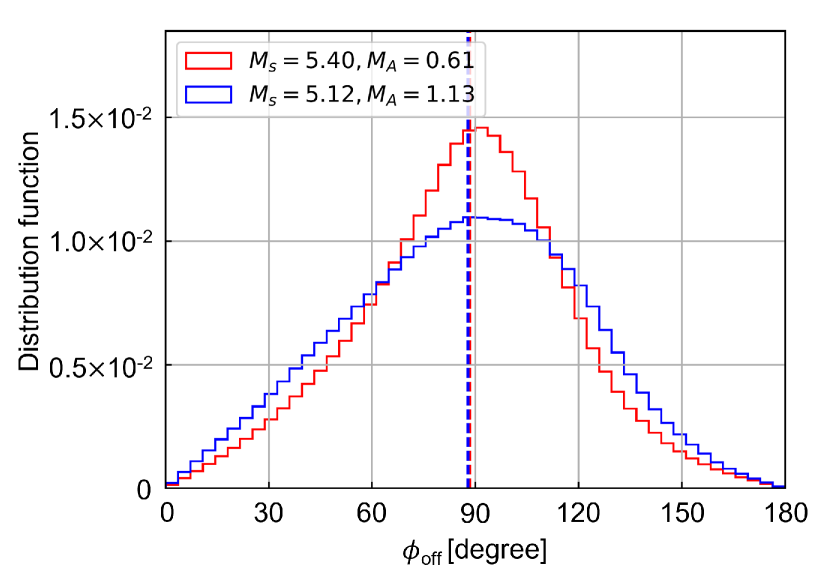
Figure 3: Histogram of the relative angle $\phi_{\rm off}$ between the magnetic field fluctuation $\delta\boldsymbol{B}$ and mean magnetic field $\langle\boldsymbol{B}\rangle$. Dashed line indicates the median value. Mean inclination angle in the simulations is $90^{\circ}$.

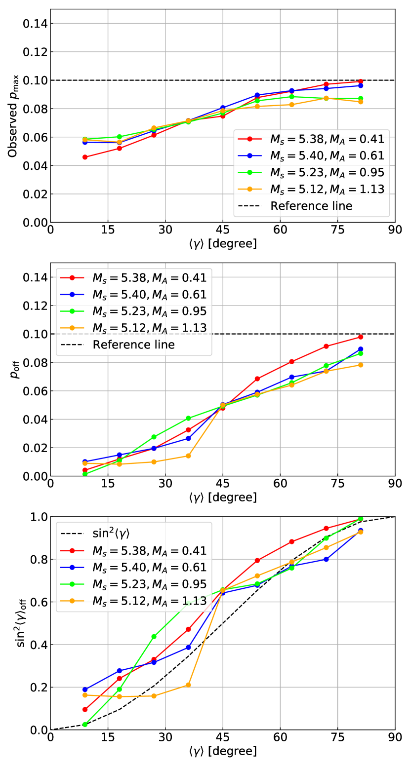
Figure 4: The observed $p_{\rm max}$ (top), $p_{\rm off}$ (middle), and estimated $\sin^{2}\langle\gamma\rangle_{\rm off}$ (bottom) as a function of the actual mean inclination angle $\langle\gamma\rangle$. The reference lines in the top two panels represent the intrinsic polarization fraction in simulations.

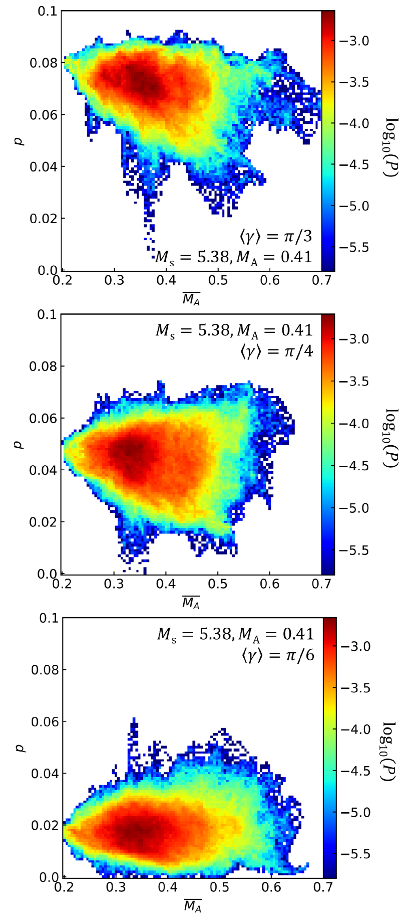
Figure 5: 2D histogram of polarization fraction $p$ and averaged total Alfvén Mach number $\overline{M_{\rm A}}$ in the conditions of various mean inclination angle $\langle\gamma\rangle$. $P$ denotes the percent of sampling points.

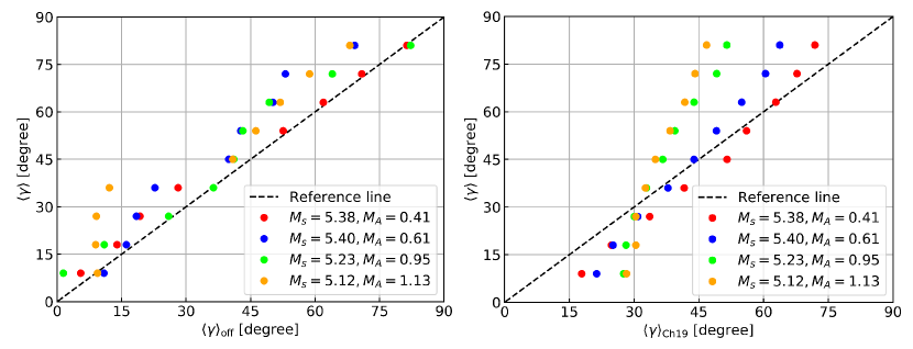
Figure 6: Comparison of the mean inclination angle $\langle\gamma\rangle_{\rm off}$/ $\langle\gamma\rangle_{\rm Ch19}$ (left/right) with the real inclination angle $\langle\gamma\rangle$ of the simulation. $\langle\gamma\rangle_{\rm off}$ is derived in this work, while $\langle\gamma\rangle_{\rm Ch19}$ was proposed by Chen et al. (2019).

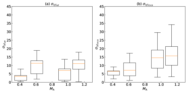
Figure 7: Deviation of estimated inclination angle and actual inclination angle. Upper and lower black lines represent the deviation’s maximum and minimum, respectively. Box gives ranges of the first (lower) and third quartiles (upper) and orange line represent the median value. Panel a: $\sigma_{\langle\gamma\rangle_{\rm off}}$ in degrees represents the absolute difference between $\langle\gamma\rangle_{\rm off}$ and $\langle\gamma\rangle$. Panel b: $\sigma_{\langle\gamma\rangle_{\rm Ch19}}$ in degrees is for the absolute difference of $\langle\gamma\rangle_{\rm Ch19}$ and $\langle\gamma\rangle$.

The relative orientation between the measured inclination angle and real inclination angle of the simulation is measured with the Alignment Measure (AM; González-Casanova & Lazarian 2017), defined as:

$${\rm AM}=2(\langle\cos^{2}\theta_{r}\rangle-\frac{1}{2}),$$ (26)

where $\theta_{r}$ is the relative angle between two vectors. AM is an averaged quantity, and its value is in the range of [-1, 1]. AM = 1 indicates that two sets of vectors are parallel, and AM = -1 denotes that the two are orthogonal.

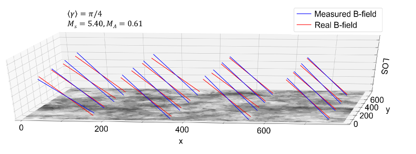
Figure 8: An example of the inclination angles measured for sixteen sub-regions with size $198\times 198$ cell². Each magnetic field vector is constructed by the POS magnetic field’s position angle (i.e., $\psi+\pi/2$) inferred from Stokes parameters and the inclination angle of either measured $\langle\gamma\rangle_{\rm off}$ (blue) or actual $\langle\gamma\rangle_{\rm sub}$ (red). Note that the obtained magnetic field is the projection along the LOS. The third axis of LOS is for 3D visualization purposes having no distance information here. The total intensity map $I$ is placed on the POS, i.e., the $x-y$ plane. The axis’s length ratio is 1:1:1 when plotting the vectors.

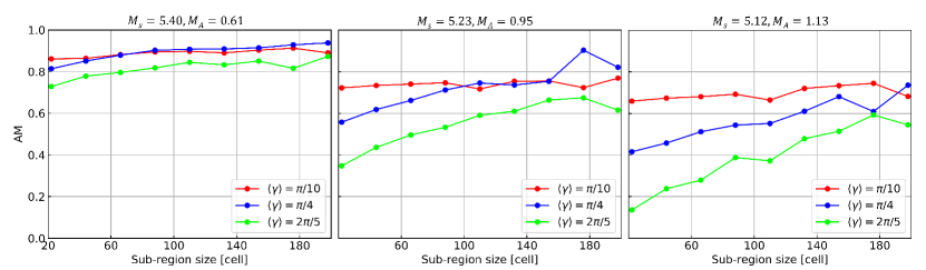
Figure 9: The AM of $\langle\gamma\rangle_{\rm off}$ and $\langle\gamma\rangle_{\rm sub}$ as a function of the sub-region’s size. $\langle\gamma\rangle$ denotes the global mean inclination angle of the full simulation box.

4 Results

4.1 The relative angle of mean magnetic field and fluctuations

Fig. 3 presents the histogram of the relative angle $\phi_{\rm off}$ between the magnetic field fluctuation $\delta\boldsymbol{B}$ and mean magnetic field $\langle\boldsymbol{B}\rangle$. The adopted simulations consist of compressible turbulence rather than only incompressible turbulence. However, we can see that for both sub-Alvénic and super-Alvénic cases, the histogram is close to a nearly symmetric distribution with a median value concentrated on $90^{\circ}$ around. The super-Alvénic case has a larger dispersion due to relatively stronger turbulence.

This median value of $\phi_{\rm off}\approx 90^{\circ}$ is crucial for our assumption that the magnetic field’s fluctuation preferentially appears in the mean field’s perpendicular direction. This assumption is also valid in compressible turbulence.

4.2 Effect of $p_{\rm max}$’s underestimation

Eq. 10 is crucial in deriving the inclination angle using Eq. 17. It requires the value of $p_{\rm max}$, which corresponds to the case of local inclination angle $\sim 90^{\circ}$, to estimate the intrinsic polarization fraction $p_{0}$. In a real scenario, this might not always be achieved. When the mean inclination angle is small, it is more difficult to locally achieve $\sim 90^{\circ}$ . The only available information in observation is the maximum value of observed $p$, which does not necessarily correspond to the case that local inclination angle $\sim 90^{\circ}$. Therefore, for practical application, we can only generalize Eq. 10 to the maximum value of observed $p$ and we denote this value as the observed $p_{\rm max}$. This generalization might underestimate $p_{0}$ and introduce uncertainty to the estimated mean inclination angle.

In Fig. 4, we study the effect of $p_{\rm max}$’s underestimation in calculating $\sin^{2}\langle\gamma\rangle_{\rm off}$ assuming homogeneous dust properties. The maximum intrinsic polarization fraction in simulations is $\sim 0.1$. However, we can see that the observed $p_{\rm max}$ achieves this value $\sim 0.1$ only when the mean inclination angle $\langle\gamma\rangle$ is larger than $\sim 60^{\circ}$. When $\langle\gamma\rangle<60^{\circ}$, the observed $p_{\rm max}$ rapidly decreases to $\sim 0.05$, because local inclination angle cannot achieve $\sim 90^{\circ}$. However, we find the decreasing trend of observed $p_{\rm max}$ when $\langle\gamma\rangle$ gets smaller is independent of $M_{\rm A}$, which characterizes the significance of magnetic field strength’s fluctuation, i.e., strength of the fluctuations relative to the strength of the mean field, across the cloud. This suggests that the major depolarization agent is the inclination angle rather than magnetic field strength’s fluctuation.

In addition to the observed $p_{\rm max}$, the value of $p_{\rm off}$ is also required to calculate $\sin^{2}\langle\gamma\rangle_{\rm off}$ (see Eq. 17). Here we obtain $p_{\rm off}$ from the polarization fraction corresponding to the minimum of $\overline{M_{\rm A}}_{,\bot}$. Due to statistically sufficient samples in the simulation, this choice satisfies the condition that $\overline{M_{\rm A}}_{,\bot}^{2}\ll 1$. As shown in Fig.4, $p_{\rm off}$ rapidly decreases in the case of small $\langle\gamma\rangle$. $p_{\rm off}$ is already close to $\sim 0$ when $\langle\gamma\rangle<10^{\circ}$. Similar to the case of observed $p_{\rm max}$, $p_{\rm off}$ has little dependence on $M_{\rm A}$.

Moreover, we find the calculated value of $\sin^{2}\langle\gamma\rangle_{\rm off}$ well follows the reference line of $\sin^{2}\langle\gamma\rangle$ when $\langle\gamma\rangle>45^{\circ}$. $\sin^{2}\langle\gamma\rangle_{\rm off}$ deviates more for small $\langle\gamma\rangle$ due to the underestimation of $p_{\rm max}$. We will quantify this uncertainty in the following.

4.3 Inclination angle as the major depolarization agent

In general, in addition to the mean inclination angle and its fluctuation, magnetic field strength’s fluctuation also contributes to the depolarization effect. However, as we see in Fig. 4, the inclination angle dominates the depolarization, while magnetic field strength’s fluctuation gives an insignificant contribution. Moreover, the supersonic simulations of compressible MHD turbulence used in Fig. 4 consist of significant density fluctuations. The observed $p_{\rm max}$, however, still achieves $\sim 0.1$ when $\langle\gamma\rangle>75^{\circ}$. It suggests that density fluctuation contributes little to depolarization.

Fig. 5 presents the 2D histograms of polarization fraction $p$ and averaged total Alfvén Mach number $\overline{M_{\rm A}}$ along the LOS using the simulation A0. The histogram concentrates in a narrow range of $p$ when $\overline{M_{\rm A}}$ is relatively small, i.e., approximately $<0.4$. The histogram spreads to a wider range of $p$ when $\overline{M_{\rm A}}>0.4$. This more dispersed correlation is mainly caused by the inclination angle’s fluctuation instead of magnetic field strength’s fluctuation. When $\overline{M_{\rm A}}$ is large, significant fluctuations appear in both inclination angle and magnetic field strength. Because the inclination angle is the major agent for depolarization, its fluctuation, in this case, causes a rapid variation of $p$. Also, due to this effect, the observed $p_{\rm max}$ is more likely to appear in a position with relatively large $\overline{M_{\rm A}}$. This position locally achieves a large inclination angle so that the depolarization effect is relatively weak.

4.4 Comparison with Chen et al. (2019)

Fig. 6 presents the comparison of the full simulation cube’s mean inclination angle obtained from Eq. 17 with the one calculated from Chen et al. (2019)’s method. For $\langle\gamma\rangle_{\rm off}$ calculated through our method, generally, it is well compatible with the actual inclination angle $\langle\gamma\rangle$ of the simulation, although $\langle\gamma\rangle_{\rm off}$ gives slightly underestimated values. This underestimation might come from two reasons: (i) the underestimation of $p_{\rm max}$ as we discussed above; (ii) density fluctuation in compressible turbulence. Eq. 17 is derived from the condition of incompressible turbulence, which contains no density fluctuation. It is possible that density fluctuation introduces uncertainties, although not significant.

As for Chen et al. (2019)’s method, its estimation agrees with $\langle\gamma\rangle$ better in strong magnetic field cases, i.e., sub-Alfvénic $M_{\rm A}=0.41$ and $0.61$. $\langle\gamma\rangle_{\rm Ch19}$, however, significantly deviates from $\langle\gamma\rangle$ when $M_{\rm A}>0.61$. This is caused by significant fluctuations in weakly magnetized turbulence, which breaks Chen et al. (2019)’s assumption that the fluctuations are negligible.

Fig. 7 shows the deviation of the estimated inclination angle and actual angle. We calculate the absolute difference between $\langle\gamma\rangle_{\rm off}$ (or $\langle\gamma\rangle_{\rm Ch19}$) and $\langle\gamma\rangle$. The calculation is performed over all data points shown in Fig. 6 and we denotes the difference as $\sigma_{\langle\gamma\rangle_{\rm off}}$ (or $\sigma_{\langle\gamma\rangle_{\rm Ch19}}$). Generally we see that the median value of $\sigma_{\langle\gamma\rangle_{\rm Ch19}}$ monotonically increases when $M_{\rm A}$ increases. It increases from $\approx 6^{\circ}$ ($M_{\rm A}=0.41$) to $\approx 15^{\circ}$ ($M_{\rm A}=1.13$). The trend of $\sigma_{\langle\gamma\rangle_{\rm off}}$’s median value is more complicated. It is similar to $\sigma_{\langle\gamma\rangle_{\rm Ch19}}$ in sub-Alfvénic case $M_{\rm A}<0.61$. In trans- and super-Alfvénic cases, $\sigma_{\langle\gamma\rangle_{\rm off}}$’s median stays in $10^{\circ}$ around. In addition to median value, the maximum $\sigma_{\langle\gamma\rangle_{\rm Ch19}}$ significantly increases to $\sim 35^{\circ}$ in trans- and super-Alfvénic conditions, which comes from $\langle\gamma\rangle_{\rm Ch19}$’s underestimation in large $\langle\gamma\rangle$ cases (see Fig. 6). In general, $\sigma_{\langle\gamma\rangle_{\rm off}}$ ranges from 0 to $\sim 20^{\circ}$ with a median value $\leq 10^{\circ}$, while $\sigma_{\langle\gamma\rangle_{\rm Ch19}}$ is in the range of 0 to $\sim 35^{\circ}$.

4.5 Sub-region sampling

As discussed above, our method mainly depends on three conditions: (i) the existence of a mean magnetic field; (ii) the existence of a reference position with $\overline{M_{\rm A}}_{,\bot}^{2}\ll 1$; (iii) the number of the sample within a region is sufficient so that perpendicular magnetic field fluctuations dominate. Thus, it is not necessary to perform the calculation to the full cloud or simulation. This method can be generalized to sub-regions satisfied with the conditions. In this section, we test the relation of $\langle\gamma\rangle_{\rm off}$’s accuracy and the sub-regions size.

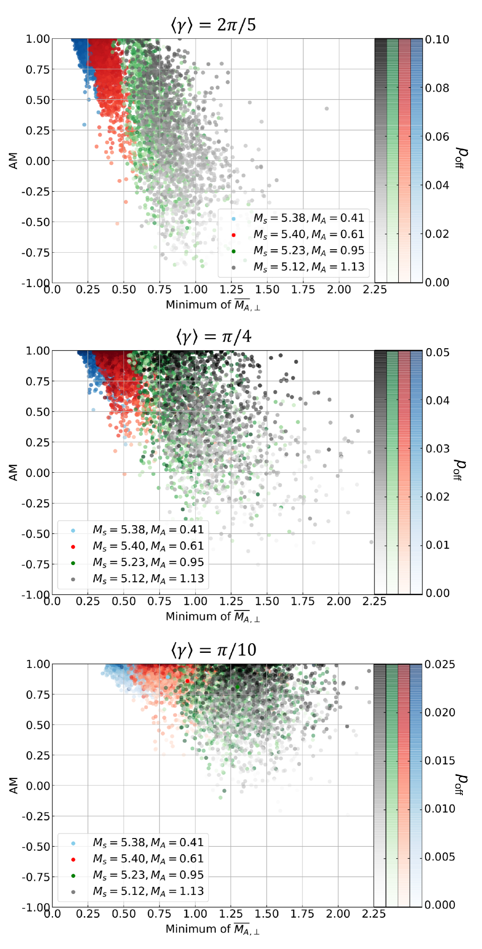
Figure 10: Scatter plots of minimum ${\overline{M_{\rm A}}_{,\bot}}$ and AM (of $\langle\gamma\rangle_{\rm off}$ and $\langle\gamma\rangle_{\rm sub}$). Minimum $\overline{M_{\rm A}}_{,\bot}$ and AM are calculated for each $22\times 22$ cell² sub-region. Color indicates the polarization fraction $p_{\rm off}$ corresponding to minimum ${\overline{M_{\rm A}}_{,\bot}}$. $\langle\gamma\rangle$ denotes the global mean inclination angle of the full simulation box.

Fig. 8 present an example of the inclination angles measured for sixteen sub-regions, whose size is $198\times 198$ cell². For simplicity, the sub-region is defined as a square, and we refer to its size using the length scale in the following. Each vector is constructed by the POS magnetic field’s position angle (i.e., $\psi+\pi/2$) inferred from Stokes parameters (see § 2) and the inclination angle of either measured $\langle\gamma\rangle_{\rm off}$ or actual $\langle\gamma\rangle_{\rm sub}$ of that sub-region. As we see, globally, the simulation has inclination $\langle\gamma\rangle=\pi/4$ and the POS magnetic field is along the $x$-axis. While the magnetic field’s orientation exhibits slight variation for each sub-region, the measured inclination angles agree well with the actual angles.

Moreover, we test the accuracy of $\langle\gamma\rangle_{\rm off}$ with various sub-region sizes. The global agreement of $\langle\gamma\rangle_{\rm off}$ and $\langle\gamma\rangle$ is quantified by the AM (see § 3). As shown in Fig. 9, in general, the AM increases for a large sub-region size. This can be easily understood as a large sub-region means the probability of finding out $\min\{\overline{M_{\rm A}}_{,\bot}^{2}\}\ll 1$ increases. Therefore, the estimation for a large sub-region is always more accurate. Also, we note that in the super-Alfvénic case (i.e., $M_{\rm A}=1.13)$, the increment of AM at a large sub-region is more significant than the sub-Alfvénic case. This indicates that the accuracy of the estimated inclination angle mainly depends on the condition that whether there exists a position with $\overline{M_{\rm A}}_{,\bot}^{2}\ll 1$. As super-Alfvénic turbulence has significant magnetic field fluctuations, it is possible that in several positions, the local physical condition becomes sub-Alfvénic. Consequently, the probability of finding out a position with $\overline{M_{\rm A}}_{,\bot}^{2}\ll 1$ increases in a large sub-region.

In addition, we notice that the estimation of $\langle\gamma\rangle_{\rm off}$ is more accurate when the actual mean inclination angle $\langle\gamma\rangle$ is small. Intuitively this disagrees with our theoretical consideration that large $\langle\gamma\rangle$ suggests a small value of $\overline{M_{\rm A}}_{,\bot}$, which better constrains $\langle\gamma\rangle_{\rm off}$. However, the crucial term in determining $\langle\gamma\rangle_{\rm off}$ is $\overline{M_{\rm A}}_{,\bot}^{2}\sin^{2}\overline{\gamma}$ instead of $\overline{M_{\rm A}}_{,\bot}^{2}$ (see Eq. 14). The choice of using $\overline{M_{\rm A}}_{,\bot}^{2}\ll 1$ is based on the fact it is the only achievable variable in observation. For a given $\overline{M_{\rm A}}$ value, a small inclination angle significantly and non-linearly reduces the value of $\overline{M_{\rm A}}_{,\bot}^{2}\sin^{2}\overline{\gamma}$. For instance, $\sin^{2}(\pi/10)$ is one order of magnitude smaller than $\sin^{2}(2\pi/5)$. Therefore, $\sin^{2}\overline{\gamma}$ becomes the leading factor when the mean inclination angle is small and consequently, Eq. 17 is better constrained with a small inclination angle.

Fig. 10 presents the relation of $\min\{\overline{M_{\rm A}}_{,\bot}\}$ and the AM (of $\langle\gamma\rangle_{\rm off}$ and $\langle\gamma\rangle_{\rm sub}$) calculated for each $22\times 22$ cell² sub-region. $\min\{\overline{M_{\rm A}}_{,\bot}\}$ is the minimum value of $\overline{M_{\rm A}}_{,\bot}$ within one sub-region. The sub-region $22\times 22$ cell² cells guarantees sufficient samples for characterizing overall statistical properties. First of all, as we expected, a small value of $\min\{\overline{M_{\rm A}}_{,\bot}\}$ is associated with large AM, i.e., high accuracy, as well large polarization fraction.

For the case of $\langle\gamma\rangle=2\pi/5$, the AM starts dropping to negative when $\min\{\overline{M_{\rm A}}_{,\bot}\}>0.50$. In this situation, the contribution from $\overline{M_{\rm A}}_{,\bot}^{2}\sin^{2}\overline{\gamma}$ is not negligible so that the assumption of Eq. 17 breaks. A smaller inclination angle $\langle\gamma\rangle=\pi/10$ shifts $\min\{\overline{M_{\rm A}}_{,\bot}\}$ to larger value and increases AM. For such a small $\langle\gamma\rangle$, $\overline{M_{\rm A}}_{,\bot}$ is less important in determining $\langle\gamma\rangle_{\rm off}$. In observation, $\langle\gamma\rangle_{\rm off}$ can be obtained from Eq. 17 targeting on the full cloud. Once the value of $\langle\gamma\rangle_{\rm off}$ is available, the sub-region size can be selected accordingly. One should use a pretty large size when both $\min\{\overline{M_{\rm A}}_{,\bot}\}>0.5$ and $\langle\gamma\rangle_{\rm off}$ is large (for instance, $\langle\gamma\rangle_{\rm off}>\pi/4$). Otherwise, if $\langle\gamma\rangle_{\rm off}$ is small, the restriction on $\min\{\overline{M_{\rm A}}_{,\bot}\}$ and sub-region size can be released. Note that in real observation that $\overline{M_{\rm A}}_{,\bot}$’s estimation also has uncertainty. Therefore, unlike our numerical results of using the $\min\{\overline{M_{\rm A}}_{,\bot}\}$ in Fig. 10, it is better to search for a number of reference positions satisfying $\overline{M_{\rm A}}_{,\bot}^{2}\ll 1$ and check the corresponding polarization fraction and inclination angle’s variation.

5 Discussion

5.1 Assumption and uncertainty

In this work, we propose a method, i.e., the Polarization Fraction Analysis (PFA), to estimate the mean inclination angle of a cloud $\langle\gamma\rangle$. This method is based on several important assumptions. First of all, we assume the existence of a mean magnetic field and the mean field’s variation along the LOS is small. This is typically valid for cloud-scale, clump-scale, and core-scale objects. We generally call these objects clouds in the paper. Secondly, we assume the intrinsic polarization fraction $p_{0}$ is constant throughout a cloud. This implicitly requires that dust grains’ properties, i.e., emissivity, temperature, etc., are homogeneous within the cloud. The other important assumptions related to incompressible MHD turbulence and uncertainty from the underestimation of $p_{\rm max}$ are discussed below.

5.1.1 Incompressible and compressible MHD turbulence

Our proposed method accommodates magnetic field fluctuations along the LOS considering incompressible MHD turbulence. This consideration builds up a simple magnetic field model, i.e., the fluctuation is dominantly along the direction perpendicular to the mean magnetic field.

The existence of a mean magnetic field implicitly assumes the MHD turbulence is sub- or trans-Alfvénic. Super-Alfvénic MHD turbulence is typically isotropic, and a mean field cannot be well defined. Nevertheless, as turbulence cascades to small scales, the importance of magnetic backreaction gets stronger. Eventually, at and below the scale $l_{\rm A}=L_{\rm inj}M_{\rm A}^{-3}$, the turbulent velocity becomes equal to the Alfvén velocity, and the turbulence becomes anisotropic (Lazarian, 2006). Therefore, for the application to a globally super-Alfvénic cloud, it is necessary that the telescope can resolve the scale smaller than $l_{\rm A}$.

Moreover, in a real scenario, ISM turbulence consists of compressible fast and slow modes. Nevertheless, both slow and fast modes in low-$\beta$ plasma are highly anisotropic (Cho & Lazarian, 2003; Kandel et al., 2017), i.e., the most significant fluctuations appear in the perpendicular direction. Here $\beta=2(\frac{M_{\rm A}}{M_{s}})^{2}$ is plasma’s compressibility. It suggests that in low-$\beta$ molecular clouds, our assumption about perpendicular magnetic field fluctuation is still valid in compressible turbulence. This is also numerically confirmed in Fig. 3.

The slow mode in high-$\beta$ plasma is similar to the pseudo-Alfvén mode in the incompressible regime, while the high-$\beta$ fast mode is a purely compressible mode with an isotropic power spectrum. Although the maximum energy fraction of fast mode is only $\sim 20\%$ (Hu et al., 2022b), an additional consideration is probably necessary to deal with the isotropic fast mode in high-$\beta$ MHD turbulence.

In addition, incompressible MHD turbulence implicitly means the absence of density fluctuations that are not negligible in observation. However, as shown in Fig. 4, the leading factor of depolarization is inclination angle, rather than density fluctuation and magnetic field strength’s fluctuation. This suggests that the density fluctuation’s role is insignificant even in supersonic turbulence.

5.1.2 Underestimation of $p_{\rm max}$

$p_{0}$ is a key parameter in deriving the inclination angle. Chen et al. (2019) argued that $p_{0}$ depends purely on the intrinsic properties of dust grain and can be calculated from $p_{0}=3p_{\rm max}/(3+p_{\rm max})$, where $p_{\rm max}$ is the ideal maximum polarization fraction corresponding to local inclination angle $\sim 90^{\circ}$. The observed $p_{\rm max}$ in observation, however, might not satisfy the condition. Consequently, the observed $p_{\rm max}$ is underestimated compared with the ideal value. As shown in Fig. 4, this underestimation is more significant when $\langle\gamma\rangle<45^{\circ}$ and it introduces uncertainty to the estimated inclination angle.

All the assumptions mentioned above can cause systematic uncertainties in the PFA. As we numerically studies in Fig. 7, the total systematic uncertainty ranges from 0 to $20^{\circ}$ with a median value $\leq 10^{\circ}$.

Moreover, the estimated inclination angle is in the range of [0, $90^{\circ}$] (see Eq. 17). It does not distinguish whether magnetic field is oriented in the first and third quadrants, as defined in Fig. 1, or in the second and fourth quadrants. This degeneracy potentially can be solved by the recent development of Faraday rotation method (Tahani et al., 2022).

5.2 Mapping the POS $M_{\rm A}$ distribution

The proposed method of probing three-dimensional magnetic fields requires maps of observed polarization fraction and $\overline{M_{\rm A}}_{,\bot}$ distribution. We list several approaches of getting $\overline{M_{\rm A}}_{,\bot}$ here.

The first way is using the polarization measurement. For instance, Falceta-Gonçalves et al. (2008) suggested a generalization of the Davis–Chandrasekhar–Fermi method (Davis, 1951; Chandrasekhar & Fermi, 1953) to obtain the $\overline{M_{\rm A}}_{,\bot}$ by $\tan\delta\theta\sim\overline{M_{\rm A}}_{,\bot}$. Here $\delta\theta$ is the dispersion of polarization angles.

Also, the $\overline{M_{\rm A}}_{,\bot}$ can be calculated from the polarization fraction using the relation $\sigma_{\rm pol\%}\sim\overline{M_{\rm A}}_{,\bot}^{2}$ (Lazarian et al., 2018), where $\sigma_{\rm pol\%}$ is the dispersion of polarization fraction. Although the measurement of $\delta\theta$ or $\sigma_{\rm pol\%}$ over a region reduces the observation’s resolution, once the $\overline{M_{\rm A}}_{,\bot}$ distribution is available, as presented in Lazarian et al. (2018), Hwang et al. (2021) and Li et al. (2021), one can access the three-dimensional magnetic field using our proposed PFA.

The velocity gradient technique (VGT; González-Casanova & Lazarian 2017; Lazarian & Yuen 2018a; Hu et al. 2018) and the structure-function analysis (SFA; Hu et al. 2021a; Xu & Hu 2021; Hu et al. 2021c) are other two approaches of getting $\overline{M_{\rm A}}_{,\bot}$. The VGT relies on the fact that velocity gradient’s dispersion is small in a strongly magnetized medium, but becomes large in weak magnetized medium. The relation of velocity gradient’s dispersion and $\overline{M_{\rm A}}_{,\bot}$ is given in Lazarian et al. (2018).

The SFA estimates $\overline{M_{\rm A}}_{,\bot}$ from the ratio of velocity fluctuations perpendicular and parallel to the POS magnetic field. Its foundation is also MHD turbulence’s anisotropy, which suggests that the maximum velocity fluctuation appears in the direction perpendicular to the magnetic field, but the minimum appears in the parallel direction. Their ratio is positively proportional to $(\overline{M_{\rm A}}_{,\bot})^{-4/3}$.

Moreover, the VGT and SFA potentially contain the necessary information for getting pixelized distributions of total magnetic field strength and inclination angle from the Eq. 11. The dilemma of Eq. 11 is that we need sufficient samples to constrain turbulence’s property, which does not appear in a single data point of dust polarization. However, the Doppler-shifted lines used by the VGT or SFA usually has a higher resolution than polarization measurement. For example, the CO (1-0) emission line observed with the Green Bank Telescope achieves a beam resolution $\sim 8^{\prime\prime}$. If one selects a sub-region size smaller than $80\times 80$ cell², the measured turbulence’s property by the VGT or SFA for each sub-region would have resolution $\sim 10^{\prime}$, which is comparable with the Planck polarization measurement. This information, therefore, could be implemented in Planck polarization to obtain local magnetic field strength and inclination angle.

5.3 Comparison with Other Methods

Chen et al. (2019) proposed a method to calculate the inclination angle of the magnetic field. Assuming idealistic and homogeneous physical conditions, i.e., magnetic field’s fluctuations are negligible, $p_{0}$ is constant across the cloud, and dust grains’ properties are the same, their method calculates the inclination angle distribution using the local polarization fraction (see Eq. 12). However, the assumption holds only for the strongly sub-Alfvénic case, while molecular clouds are typically trans-Alfvénic or super-Alfvénic (Federrath et al., 2016; Hu et al., 2019; Hwang et al., 2021; Li et al., 2021; Tram et al., 2022). The systematic uncertainty of their method in trans-Alfvénic or super-Alfvénic regimes ranges from $\sim 3^{\circ}$ to $\sim 35^{\circ}$.

In this work, we take into account the fluctuation of the magnetic field due to anisotropic MHD turbulence. We show that the local polarization fraction, in this case, depends on not only the inclination angle but also the magnetic field fluctuation. The fluctuation amplifies the depolarization effect. Consequently, the local polarization fraction does not accurately characterize the inclination angle using Eq. 12. We propose and demonstrate that the polarization fraction in the reference position with $\overline{M_{\rm A}}_{,\bot}^{2}\ll 1$ is determined by the mean inclination angle over a region of interest since the contribution from the fluctuation is insignificant there. The mean inclination angle thus can be calculated (see Eq. 17) once the distribution of $\overline{M_{\rm A}}_{,\bot}^{2}$ is available. In particular, our method is applicable to molecular clouds. Because trans-Alfvénic or super-Alfvénic clouds raise significant $\overline{M_{\rm A}}_{,\bot}$ fluctuations, one can easily find a position corresponding to $\overline{M_{\rm A}}_{,\bot}^{2}\ll 1$ by searching for sufficient samples.

Another two methods of tracing three-dimensional magnetic fields were proposed by Hu et al. (2021a) and Hu et al. (2021c). The two methods are based on MHD turbulence’s anisotropic property, i.e., the maximum velocity fluctuation appears in the direction perpendicular to the magnetic field. Consequently, by measuring the three-dimensional velocity fluctuations of young stellar objects, which are accessible via the Gaia survey (Gaia Collaboration et al., 2016, 2018; Ha et al., 2021; Ha et al., 2022), one can find the three-dimensional magnetic fields (Hu et al., 2021a). Hu et al. (2021c), on the other hand, proposed to measure the velocity fluctuations using Doppler-shifted emission lines. It was shown that the ratio of maximum and minimum fluctuations within a given velocity channel is correlated with the velocity channel width, total Alfvén Mach number, and the inclination angle. Therefore, by varying the channel widths used for calculating the ratio, one can solve the $M_{\rm A}$ and inclination angle simultaneously.

6 Summary

Dust polarization is one of the most important ways to trace the magnetic fields in ISM. We propose a new method, i.e., the PFA, to trace three-dimensional magnetic fields using the observed polarization fraction of polarized dust emission and the distribution of the POS Alfvén Mach number. This method mainly assumes the existence of a mean magnetic field in a physically homogeneous cloud and magnetic field fluctuations arise from anisotropic MHD turbulence. We summarize as follows:

1. We numerically confirm that magnetic fluctuation of compressible turbulence dominantly appears in the direction perpendicular to the mean magnetic field.

2. We find inclination angle is the primary agent for depolarization. Fluctuations of magnetic field strength and density have an insignificant contribution.

3. We analytically propose and numerically confirm that the polarization fraction corresponding to $\overline{M_{\rm A}}_{,\bot}^{2}\ll 1$ can characterize the mean inclination angle.

4. We test the PFA using 3D compressible MHD turbulence simulations and show that it is applicable to sub-Alfvénic, trans-Alfvénic, and moderately supers-Alfvénic clouds with $0.4\lesssim M_{\rm A}\lesssim 1.2$.

5. We numerically find the PFA has systematic uncertainty ranging from 0 to $20^{\circ}$ with a median value $\leq 10^{\circ}$.

Data Availability

The data underlying this article will be shared on reasonable request to the corresponding author.

Appendix A 3D Turbulent velocity estimated from emission line

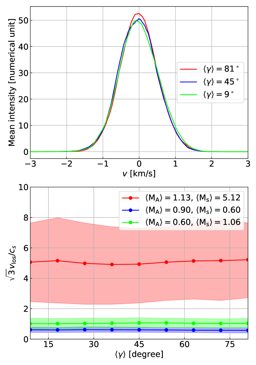
Figure 11: Top: synthetic spectra generated from the simulation $\langle M_{\rm A}\rangle=1.13,\langle M_{\rm s}\rangle=5.12$ with various $\langle\gamma\rangle$. Bottom: the correlation of median $\sqrt{3}v_{\rm los}/c_{s}$ and mean inclination angle $\langle\gamma\rangle$. $c_{s}\approx 0.192$ is the speed of sound in numerical unit. The shadowed area indicates the ranges of one-sigma level.

To find the distribution of $\overline{M_{\rm A}}_{,\bot}$, knowledge of turbulent velocity $v_{l}=(l/L_{\rm inj})^{1/3}v_{\rm inj}$ at scale $l$ is required, assuming Kolmogorov-type turbulence. Here $L_{\rm inj}$ is the injection scale and $v_{\rm inj}=\sqrt{3}v_{\rm los}$ is the 3D turbulent velocity at injection scale. This calculation needs the emission line’s width $v_{\rm los}$ and isotropic turbulence at the injection scale.

We use three numerical simulations $\langle M_{\rm A}\rangle=1.13,\langle M_{\rm s}\rangle=5.12$, $\langle M_{\rm A}\rangle=0.90,\langle M_{\rm s}\rangle=0.60$, and $\langle M_{\rm A}\rangle=0.60,\langle M_{\rm s}\rangle=1.06$ to test the validity of $v_{\rm inj}=\sqrt{3}v_{\rm los}$ with different $\langle\gamma\rangle$. The simulation setup is the same as the one presented in § 3.

We extract the LOS velocity and density information from MHD simulations to generate synthetic Position-Position-Velocity (PPV) cubes. Fig. 11 presents the spectra calculated from the PPV cubes generated from the simulation $\langle M_{\rm A}\rangle=1.13,\langle M_{\rm s}\rangle=5.12$ in the conditions of $\langle\gamma\rangle=81^{\circ}$, $\langle\gamma\rangle=45^{\circ}$, and $\langle\gamma\rangle=9^{\circ}$. The spectra are averaged over the full PPV cubes along the $x$ and $y$-directions, i.e., the POS. We ensure that the same number of pixels enter the calculations and that the spectra are calculated in the same interval and with the same bandwidth. We can see the spectral width has insignificant changes. Moreover, we calculate $v_{\rm los}$ from $v_{\rm los}={\rm FWHM}/\sqrt{8\ln{2}}$, where ${\rm FWHM}$ stands for the full width at half maximum. The FWHM is independently calculated for the spectrum in each pixel. The median value of $\sqrt{3}v_{\rm los}/c_{s}$ gives an estimation of the simulation’s intrinsic $\langle M_{s}\rangle$ at injection scale. In Fig. 11, we can see, in all sub-sonic, trans-sonic, and supersonic conditions, $\sqrt{3}v_{\rm los}/c_{s}$ has only insignificant variation when $\langle\gamma\rangle$ changes. However, although we expect isotropic turbulence driving in most cases, readers should be careful about the situation of anisotropic driving. Anisotropic driving would result in either an underestimation or overestimation of $\overline{M_{\rm A}}_{,\bot}$ using the relation $v_{\rm inj}=\sqrt{3}v_{\rm los}$.

References

- Abbate et al. (2020) Abbate F., Possenti A., Tiburzi C., Barr E., van Straten W., Ridolfi A., Freire P., 2020, Nature Astronomy, 4, 704
- Allen et al. (2003) Allen A., Li Z.-Y., Shu F. H., 2003, ApJ, 599, 363
- Andersson et al. (2015) Andersson B. G., Lazarian A., Vaillancourt J. E., 2015, ARA&A, 53, 501
- Armstrong et al. (1995) Armstrong J. W., Rickett B. J., Spangler S. R., 1995, ApJ, 443, 209
- Beattie et al. (2022) Beattie J. R., Krumholz M. R., Federrath C., Sampson M., Crocker R. M., 2022, arXiv e-prints, p. arXiv:2203.13952
- Beresnyak & Lazarian (2019) Beresnyak A., Lazarian A., 2019, Turbulence in Magnetohydrodynamics
- Busquet (2020) Busquet G., 2020, Nature Astronomy, 4, 1126
- Chandrasekhar & Fermi (1953) Chandrasekhar S., Fermi E., 1953, ApJ, 118, 113
- Chen et al. (2019) Chen C.-Y., King P. K., Li Z.-Y., Fissel L. M., Mazzei R. R., 2019, MNRAS, 485, 3499
- Chepurnov & Lazarian (2010) Chepurnov A., Lazarian A., 2010, ApJ, 710, 853
- Cho & Lazarian (2003) Cho J., Lazarian A., 2003, MNRAS, 345, 325
- Cho & Vishniac (2000) Cho J., Vishniac E. T., 2000, ApJ, 539, 273
- Chuss et al. (2019) Chuss D. T., et al., 2019, ApJ, 872, 187
- Clark & Hensley (2019) Clark S. E., Hensley B. S., 2019, ApJ, 887, 136
- Crutcher (1999) Crutcher R. M., 1999, ApJ, 520, 706
- Crutcher (2004) Crutcher R. M., 2004, in Uyaniker B., Reich W., Wielebinski R., eds, The Magnetized Interstellar Medium. pp 123–132
- Crutcher (2012) Crutcher R. M., 2012, ARA&A, 50, 29
- Davis (1951) Davis L., 1951, Physical Review, 81, 890
- Evans (1999) Evans Neal J. I., 1999, ARA&A, 37, 311
- Falceta-Gonçalves et al. (2008) Falceta-Gonçalves D., Lazarian A., Kowal G., 2008, ApJ, 679, 537
- Fanciullo et al. (2022) Fanciullo L., et al., 2022, MNRAS, 512, 1985
- Federrath & Klessen (2012) Federrath C., Klessen R. S., 2012, ApJ, 761, 156
- Federrath et al. (2016) Federrath C., et al., 2016, ApJ, 832, 143
- Fiege & Pudritz (2000) Fiege J. D., Pudritz R. E., 2000, ApJ, 544, 830
- Fissel et al. (2016) Fissel L. M., et al., 2016, ApJ, 824, 134
- Gaia Collaboration et al. (2016) Gaia Collaboration et al., 2016, A&A, 595, A1
- Gaia Collaboration et al. (2018) Gaia Collaboration et al., 2018, A&A, 616, A1
- Ghilea et al. (2011) Ghilea M. C., Ruffolo D., Chuychai P., Sonsrettee W., Seripienlert A., Matthaeus W. H., 2011, ApJ, 741, 16
- Goldreich & Sridhar (1995) Goldreich P., Sridhar S., 1995, ApJ, 438, 763
- González-Casanova & Lazarian (2017) González-Casanova D. F., Lazarian A., 2017, ApJ, 835, 41
- Guan et al. (2021) Guan Y., et al., 2021, ApJ, 920, 6
- Ha et al. (2021) Ha T., Li Y., Xu S., Kounkel M., Li H., 2021, ApJ, 907, L40
- Ha et al. (2022) Ha T., Li Y., Kounkel M., Xu S., Li H., Zheng Y., 2022, arXiv e-prints, p. arXiv:2205.00012
- Han (2017) Han J. L., 2017, ARA&A, 55, 111
- Haverkorn (2007) Haverkorn M., 2007, in Haverkorn M., Goss W. M., eds, Astronomical Society of the Pacific Conference Series Vol. 365, SINS - Small Ionized and Neutral Structures in the Diffuse Interstellar Medium. p. 242 (arXiv:astro-ph/0611090)
- Hayes et al. (2006) Hayes J. C., Norman M. L., Fiedler R. A., Bordner J. O., Li P. S., Clark S. E., ud-Doula A., Mac Low M.-M., 2006, ApJS, 165, 188
- Hennebelle & Falgarone (2012) Hennebelle P., Falgarone E., 2012, A&ARv, 20, 55
- Higdon (1984) Higdon J. C., 1984, ApJ, 285, 109
- Hoang (2019) Hoang T., 2019, ApJ, 876, 13
- Hu & Lazarian (2022) Hu Y., Lazarian A., 2022, arXiv e-prints, p. arXiv:2210.11023
- Hu et al. (2018) Hu Y., Yuen K. H., Lazarian A., 2018, MNRAS, 480, 1333
- Hu et al. (2019) Hu Y., et al., 2019, Nature Astronomy, 3, 776
- Hu et al. (2020a) Hu Y., Yuen K. H., Lazarian A., 2020a, ApJ, 888, 96
- Hu et al. (2020b) Hu Y., Lazarian A., Bialy S., 2020b, ApJ, 905, 129
- Hu et al. (2021a) Hu Y., Xu S., Lazarian A., 2021a, ApJ, 911, 37
- Hu et al. (2021b) Hu Y., Lazarian A., Stanimirović S., 2021b, ApJ, 912, 2
- Hu et al. (2021c) Hu Y., Lazarian A., Xu S., 2021c, ApJ, 915, 67
- Hu et al. (2022a) Hu Y., Lazarian A., Wang Q. D., 2022a, MNRAS, 511, 829
- Hu et al. (2022b) Hu Y., Lazarian A., Xu S., 2022b, MNRAS, 512, 2111
- Hwang et al. (2021) Hwang J., et al., 2021, ApJ, 913, 85
- Iroshnikov (1963) Iroshnikov P. S., 1963, Azh, 40, 742
- Jokipii (1966) Jokipii J. R., 1966, ApJ, 146, 480
- Kandel et al. (2017) Kandel D., Lazarian A., Pogosyan D., 2017, MNRAS, 464, 3617
- Kowal & Lazarian (2010) Kowal G., Lazarian A., 2010, ApJ, 720, 742
- Kraichnan (1965) Kraichnan R. H., 1965, Physics of Fluids, 8, 1385
- Larson (1981) Larson R. B., 1981, MNRAS, 194, 809
- Lazarian (2006) Lazarian A., 2006, ApJ, 645, L25
- Lazarian (2007) Lazarian A., 2007, J. Quant. Spectrosc. Radiative Transfer, 106, 225
- Lazarian & Hoang (2021) Lazarian A., Hoang T., 2021, ApJ, 908, 12
- Lazarian & Pogosyan (2012) Lazarian A., Pogosyan D., 2012, ApJ, 747, 5
- Lazarian & Vishniac (1999) Lazarian A., Vishniac E. T., 1999, ApJ, 517, 700
- Lazarian & Yuen (2018a) Lazarian A., Yuen K. H., 2018a, ApJ, 853, 96
- Lazarian & Yuen (2018b) Lazarian A., Yuen K. H., 2018b, ApJ, 865, 59
- Lazarian et al. (2012) Lazarian A., Esquivel A., Crutcher R., 2012, ApJ, 757, 154
- Lazarian et al. (2018) Lazarian A., Yuen K. H., Ho K. W., Chen J., Lazarian V., Lu Z., Yang B., Hu Y., 2018, ApJ, 865, 46
- Li et al. (2021) Li P. S., Lopez-Rodriguez E., Ajeddig H., André P., McKee C. F., Rho J., Klein R. I., 2021, MNRAS,
- Mac Low & Klessen (2004) Mac Low M.-M., Klessen R. S., 2004, Reviews of Modern Physics, 76, 125
- Maron & Goldreich (2001) Maron J., Goldreich P., 2001, ApJ, 554, 1175
- McKee & Ostriker (2007) McKee C. F., Ostriker E. C., 2007, ARA&A, 45, 565
- Montgomery & Matthaeus (1995) Montgomery D., Matthaeus W. H., 1995, ApJ, 447, 706
- Montgomery & Turner (1981) Montgomery D., Turner L., 1981, Physics of Fluids, 24, 825
- Myers (1983) Myers P. C., 1983, ApJ, 270, 105
- Myers & Goodman (1988) Myers P. C., Goodman A. A., 1988, ApJ, 326, L27
- Oppermann et al. (2012) Oppermann N., et al., 2012, A&A, 542, A93
- Planck Collaboration et al. (2015a) Planck Collaboration et al., 2015a, A&A, 576, A104
- Planck Collaboration et al. (2015b) Planck Collaboration et al., 2015b, A&A, 576, A105
- Planck Collaboration et al. (2016a) Planck Collaboration et al., 2016a, A&A, 586, A136
- Planck Collaboration et al. (2016b) Planck Collaboration et al., 2016b, A&A, 586, A141
- Planck Collaboration et al. (2016c) Planck Collaboration et al., 2016c, A&A, 594, A25
- Planck Collaboration et al. (2020) Planck Collaboration et al., 2020, A&A, 641, A11
- Roche et al. (2018) Roche P. F., Lopez-Rodriguez E., Telesco C. M., Schödel R., Packham C., 2018, MNRAS, 476, 235
- Ruzmaikin et al. (1988) Ruzmaikin A. A., Sokolov D. D., Shukurov A. M., 1988, Magnetic Fields of Galaxies. Vol. 133, doi:10.1007/978-94-009-2835-0,
- Shebalin et al. (1983) Shebalin J. V., Matthaeus W. H., Montgomery D., 1983, Journal of Plasma Physics, 29, 525
- Sullivan et al. (2021) Sullivan C. H., Fissel L. M., King P. K., Chen C. Y., Li Z. Y., Soler J. D., 2021, MNRAS, 503, 5006
- Tahani et al. (2018) Tahani M., Plume R., Brown J. C., Kainulainen J., 2018, A&A, 614, A100
- Tahani et al. (2019) Tahani M., Plume R., Brown J. C., Soler J. D., Kainulainen J., 2019, A&A, 632, A68
- Tahani et al. (2022) Tahani M., et al., 2022, arXiv e-prints, p. arXiv:2201.04718
- Taylor et al. (2009) Taylor A. R., Stil J. M., Sunstrum C., 2009, ApJ, 702, 1230
- Tram et al. (2022) Tram L. N., et al., 2022, arXiv e-prints, p. arXiv:2205.12084
- Uchida & Shibata (1985) Uchida Y., Shibata K., 1985, PASJ, 37, 515
- Wang et al. (2016) Wang X., Tu C., Marsch E., He J., Wang L., 2016, ApJ, 816, 15
- Wurster & Li (2018) Wurster J., Li Z.-Y., 2018, Frontiers in Astronomy and Space Sciences, 5, 39
- Xiao et al. (2008) Xiao L., Fürst E., Reich W., Han J. L., 2008, A&A, 482, 783
- Xu & Hu (2021) Xu S., Hu Y., 2021, ApJ, 910, 88
- Xu & Yan (2013) Xu S., Yan H., 2013, ApJ, 779, 140
- Xu & Zhang (2016) Xu S., Zhang B., 2016, ApJ, 824, 113
- Yuen et al. (2022) Yuen K. H., Ho K. W., Law C. Y., Chen A., Lazarian A., 2022, arXiv e-prints, p. arXiv:2204.13760
- Zhang et al. (2020) Zhang H., Gangi M., Leone F., Taylor A., Yan H., 2020, ApJ, 902, L7
- Zielinski & Wolf (2022) Zielinski N., Wolf S., 2022, A&A, 659, A22