Estimation of Consistent Time Delays in Subsample via Auxiliary-Function-Based Iterative Updates

Abstract

In this paper, we propose a new algorithm for the estimation of multiple time delays. Since a TD is a fundamental spatial cue for sensor array signal processing techniques, many methods for estimating it have been studied. Most of them, including generalized cross correlation (CC)-based methods, focus on how to estimate a TD between two sensors. These methods can then be easily adapted for multiple TDs by applying them to every pair of a reference sensor and another one. However, these pairwise methods can use only the partial information obtained by the selected sensors, resulting in inconsistent TD estimates and limited estimation accuracy. In contrast, we propose joint optimization of entire TD parameters, where spatial information obtained from all sensors is taken into account. We also introduce a consistent constraint regarding TD parameters to the observation model. We then consider a multidimensional CC (MCC) as the objective function, which is derived on the basis of maximum likelihood estimation. To maximize the MCC, which is a nonconvex function, we derive the auxiliary function for the MCC and design efficient update rules. We additionally estimate the amplitudes of the transfer functions for supporting the TD estimation, where we maximize the Rayleigh quotient under the non-negative constraint. We experimentally analyze essential features of the proposed method and evaluate its effectiveness in TD estimation. Code will be available at https://github.com/onolab-tmu/AuxTDE.

I Introduction

A TD or time difference of arrival (TDOA) [1] observed between two sensors is a fundamental spatial cue for many signal processing techniques such as source localization, speech enhancement, and signal separation. Source localization and direction of arrival (DOA) estimation are essential techniques in audio [2, 3, 4, 5, 6] and other various engineering fields including, sonar [7], radar [8], ground-penetrating radar [9], and reflection seismology [10]. TD-based localization methods are widely studied because of its importance [11, 12, 13]. Speech enhancement is also important to extract an desired signal from noisy observation(s) [14, 15, 16]. Resampling [17, 18] and synchronization [19] are also general topics, especially for asynchronous distributed systems [20]. For these techniques, the TDs are important spatial features, where any improvement in TD estimation (TDE) directly translates to their better performance, and numerous studies exist [1, 21].

The mainstream TDE techniques are based on the generalized cross correlation (GCC) method [22], which is the most popular technique. Many techniques to improve the accuracy of GCC-based TDE have been proposed [23, 24, 25], where many studies focus on how to estimate a single TD between two different sensors. This is because we can easily adapt these techniques for an array of more than three sensors, where there are multiple TDs to be estimated, by applying them repeatedly for every pair of a reference sensor and another one. We call this simple solution the pairwise method in this paper.

Although the pairwise method is broadly used, we consider some problems. First, the CC between a sensor and another far from it may be low, which degrades the accuracy of a GCC-based method. This may be a serious problem, especially in a large-scale environment, e.g., distributed systems [20]. Second, TDs estimated by the pairwise method are inconsistent. Assuming three sensors as shown in Fig. 1, the TD between sensors $1$ and $3$ is theoretically equal to the sum of those between sensors $1$ and $2$ and $2$ and $3$. However, this does not hold true because of, for example, estimation errors caused by the presence of noise. The best sensor to use as the reference sensor and how to identify it are unclear. Summarizing the above, the pairwise method only uses partial information obtained from a pair of sensors. For better TDE, the spatial information obtained from all sensors should be taken into account. In this paper, we thus aim to develop a new method for simultaneously estimating consistent TDs to improve their estimation accuracy.

Figure 1: Time delays and a sensor array. The time delay $\tau_{13}$ is equal to the sum of time delays $\tau_{12}$ and $\tau_{23}$ physically. This relationship holds for any sensor array alignments.

Let us consider observing a source signal with an $M$ channel sensor array. The number of sensor pairs is ${}_{M}C_{2}$ ($M$ choose $2$), and the same number of TDs can be computed while only $M-1$ TDs exist theoretically; in other words, there is redundancy. Some techniques utilize this redundancy to estimate a more accurate TD, e.g., by introducing a multichannel CC coefficient [26, 27, 1]. In contrast, we introduce a consistent constraint for estimating $M-1$ TDs and consider MCC that encodes spatial cues obtained from all sensors. Here, TDE via the maximization of the MCC has two difficulties: how to attain the TD estimates with subsample precision and how to estimate them efficiently.

The methodology of subsample TDE is widely studied to improve the accuracy of GCC-based estimation [22, 23, 24]. A naïve TD estimate is given by the location of the maximum of the discrete CC function between two sensors. Without further processing, the accuracy of a GCC-based method is limited by the sampling frequency. This can be a serious problem, especially for compact arrays. For example, for a sound source radiated in an ambient atmosphere, the maximum TD observed by two microphones spaced by $4\text{\,}\mathrm{cm}$ is less than $0.12\text{\,}\mathrm{ms}$, i.e., less than two samples at $16\text{\,}\mathrm{kHz}$. Such a sample level accuracy is insufficient for many applications, including, but not limited to, audio and optical processing techniques. In the case of two sensors, interpolation is a popular and effective method to attain the subsample TD estimate, where the CC function is interpolated in the vicinity of the maximum. The parabolic interpolation [28] determines a quadratic function whose curve goes through three neighboring points, namely, the discrete maximum point of the GCC function and its two adjacent points on both sides. By using the vertex of the quadratic function instead of the discrete maximum, we can obtain a subsample TD estimate. Various schemes have been proposed, e.g., Gaussian curve fitting [29] and others [30, 31, 32]. Yet another interpolation method is zero padding in the frequency domain, which corresponds to Dirichlet kernel interpolation [33], where the ratio of nonpadded to padded signal lengths is the attainable subsample accuracy. However, these techniques attain not the maximum of the GCC funcion but an approximate one and are only applicable to the pairwise method.

It is possible to find the maximum of the continuous GCC function directly. For band-limited signals, on the basis of the Nyquist–Shannon sampling theorem [34, 35], the continuous GCC function is obtained by $\operatorname{sinc}$-interpolation of its discrete counterpart. Its maximization is a nonconvex problem without a known closed-form solution. Nevertheless, a locally optimal solution can be found with a search algorithm such as the exhaustive search scheme [36] and golden-section search (GSS) [37]. The GSS is an efficient algorithm of ternary searches, and thus, it must be performed on a two-dimensional parameter space selected from $M-1$ TD parameters in order. The exhaustive algorithm can be applied to the search in $(M-1)$-dimensional parameter space; however, it is computationally demanding.

In contrast, we previously proposed a technique of maximizing a continuous CC function via the auxiliary-function-based iterative updates for subsample TDE [38]. This technique theoretically yields the same estimate as the exhaustive search, but the computational cost is markedly low owing to efficient updates. By extending this method, in this paper, we propose an efficient algorithm, namely, auxiliary-function-based TDE (AuxTDE), for obtaining highly accurate and consistent TD estimates. First, we derive the objective function, i.e., the MCC in the maximum likelihood (ML) sense. Then, we show that the objective function can be globally bounded by a quadratic auxiliary function and can then be repeatedly maximized for guaranteed convergence to a local maximum. Finally, we propose the AuxTDE algorithm to estimate consistent TDs. This method reaches the exact peak of the objective function, which means that the highly accurate subsample estimates can be obtained, and is the reference-free algorithm, which means that consistent TDs are obtained.

The rest of this paper is organized as follows. In section II, we define the signal model and briefly introduce the GCC-method. We also define what is consistent TDs. In section III, we formulate the estimation of consistent TDs and define the objective function. In section IV, we first explain the fundamental idea and theories for our problem. We here consider the case of two sensors as the simplest scenario, where we show the relationship between the objective function and CC. In section V, we generalize the algorithm described in section IV and propose the technique for estimating consistent TDs. Experimental analysis and numerical experiments are the topics in sections VI and VII, respectively. Section VIII concludes this paper.

Note that this paper is partially based on conference paper [38] in which we proposed the technique introduced in section IV. The contribution of this paper is that we extend the proposed method in [38] to multiple TDs and introduce the concept of consistent TDs.

II Time delays estimation

II-A Signal Model

In this paper, we consider estimating every interchannel subsample TD observed by an $M$ channel sensor array. Let $x_{mkn}$ be the short-time Fourier transform (STFT) representation of the signal observed by the $m$th sensor at the discrete frequency $k$ in the $n$th time frame. We model the observations as

$$\bm{x}_{{}kn} =\tilde{\mbox{\large$s$}}_{{}kn}\bm{h}_{k}+\bm{u}_{{}kn}$$

$$=\mathopen{}\mathclose{{}\left[{x_{{1}kn}}\ \cdots\ {x_{{M}kn}}}\right]^{\mathsf{T}},$$ (1)

$$\bm{h}_{k} =\mathopen{}\mathclose{{}\left[{\tilde{a}_{1k}e^{-\mathbbm{i}\omega_{k}t_{1}}}\ \cdots\ {\tilde{a}_{Mk}e^{-\mathbbm{i}\omega_{k}t_{M}}}}\right]$$

$$=\mathopen{}\mathclose{{}\left[{h_{1k}}\ \cdots\ {h_{Mk}}}\right]^{\mathsf{T}},$$ (2)

where $\tilde{\mbox{\large$s$}}_{{}kn}$ is a source signal and $\bm{u}_{{}kn}=\mathopen{}\mathclose{{}\left[{u_{{1}kn}}\ \cdots\ {u_{{M}kn}}}\right]^{\mathsf{T}}$ is noise signals at each sensor, where the superscript $\mathsf{T}$ denotes nonconjugate transposition. $\mathbbm{i}=\sqrt{-1}$ denotes the imaginary unit, $\omega_{k}=2\pi k/T$ denotes the normalized angular frequency, and $T$ denotes the number of samples in a frame. $\bm{h}_{k}$ is the transfer function from the signal source to the sensor array, where $\tilde{a}_{mk}$ and $t_{m}$ denote the amplitude and the time of arrival (TOA), respectively. The TOA represents the absolute time when the wave propagates to the sensor from the signal source. We here consider the relative transfer function (RTF) $\bm{g}_{k}$ [39, 40], which is defined as the ratio of the transfer function $\bm{h}_{k}$:

$$\bm{g}_{{}k}\mathopen{}\mathclose{{}\left(\bm{a}_{{}k},\bm{\tau}}\right) =\bm{h}_{k}/h_{rk}$$

$$=\mathopen{}\mathclose{{}\left[{a_{1k}e^{-\mathbbm{i}\omega_{k}\tau_{1}}}\ \cdots\ {a_{Mk}e^{-\mathbbm{i}\omega_{k}\tau_{M}}}}\right]^{\mathsf{T}},$$ (3)

$$\bm{a}_{k} =\mathopen{}\mathclose{{}\left[{a_{1k}}\ \cdots\ {a_{Mk}}}\right]^{\mathsf{T}},$$ (4)

$$\bm{\tau} =\mathopen{}\mathclose{{}\left[{\tau_{r1}}\ \cdots\ {\tau_{rM}}}\right]^{\mathsf{T}},$$ (5)

where $a_{mk}=\tilde{a}_{mk}/\tilde{a}_{rk}$ is the frequency-dependent relative amplitude ($a_{mk}\in\mathbb{R}^{+}$), and $\tau_{rm}=t_{m}-t_{r}$ is the continuous TD (TDOA) between the reference sensor $r$ and the $m$th sensor. Therefore, $a_{rk}=1$ for all $k$, and $\tau_{rr}=0$. This means that degree of freedom of the TDs is $M-1$ ($M$ TOAs minus one time origin). Without loss of generality, we set to $r=1$ in this paper. Finally, the signal model (II-A) with the RTF is

$$\bm{x}_{{}kn} =\mbox{\large$s$}_{{}kn}\bm{g}_{{}k}\mathopen{}\mathclose{{}\left(\bm{a}_{{}k},\bm{\tau}}\right)+\bm{u}_{{}kn},$$ (6)

where $\mbox{\large$s$}_{{}kn}=\tilde{\mbox{\large$s$}}_{{}kn}h_{rk}$ is the source image observed at the reference sensor. Then, the objective of this paper is to estimate TDs $\bm{\tau}$ from the observations $\bm{x}_{{}kn}$. In the rest of this paper, we denote scalars by regular letters and denote vectors and matrices by bold lower and upper case letters, respectively.

II-B GCC-based Time Delay Estimation

The GCC method [22, 24] is commonly used for estimating a discrete TD that maximizes the weighted CC function

$$\Phi^{(rm)}(\tau) =\frac{1}{T}\sum_{k=-T/2+1}^{T/2}W_{k}S_{k}^{(rm)}e^{\mathbbm{i}\omega_{k}\tau},$$ (7)

$$\hat{\tau}_{rm} =\operatorname*{arg~{}max}_{\tau}\ \Phi^{(rm)}(\tau),$$ (8)

where $W_{k}\in\mathbb{R}^{+}$ is an arbitrary weight function for the GCC function and $S_{k}^{(rm)}$ is the cross spectrum of $x_{mkn}$ and $x_{rkn}$. Suitable weight functions have been proposed, e.g., GCC-PHAT (phase transform) and GCC-SCOT (smoothed coherence transform):

$$W_{k}^{\rm PHAT}=|S_{k}^{(rm)}|^{-1},\quad W_{k}^{\rm SCOT}=\mathopen{}\mathclose{{}\left(S_{k}^{(rr)}S_{k}^{(mm)}}\right)^{-\frac{1}{2}}.$$ (9)

The GCC function with $W_{k}=1$ is equivalent to the ordinary CC function. In typical implementations, the above GCC function is only computed at discrete TDs given by the sampling frequency $F_{s}$ of the input signals, i.e., $\tau_{rm}\in\mathopen{}\mathclose{{}\left\{\frac{k}{F_{s}}\,|\,k=-\frac{T}{2}+1,\ldots,\frac{T}{2}}\right\}$. To improve the accuracy, it is necessary to remove this restriction, and many methods have been proposed as described in section I.

The GCC method is easily applicable to estimating multiple TDs; namely, we repeatedly obtain the GCC function by computing (7) and maximize it by solving (8) for all $m$ except for $r$. We call this approach, which uses only partial information, the pairwise method in this paper. The algorithm of the pairwise method is quite simple, and many existing methods can be adapted; however, these TD estimates computed by the pairwise method are basically inconsistent.

II-C Consistent Time Delays

With $M$ sensors and one signal source, there are $M-1$ TDs. This means that although we need to select one reference sensor to determine the absolute time origin, the theoretical TDs are independent of its selection. In other words, the TDs should be consistent. Now, we define what are consistent TDs.

Definition 1 (Consistent time delays).

Let $\tau_{rm}$ be the time delay between $m$th ($m=1,\dots,M$) and $r$th sensors. The time delays are said to be consistent if

$$\tau_{r^{\prime}m}=\tau_{r^{\prime}r}+\tau_{rm}\ \ \forall m,r,r^{\prime},$$ (10)

where $r^{\prime}$ is another reference sensor and $r^{\prime}=1,\dots,M$.

Definition 1 is always satisfied when $\tau_{rm}=t_{m}-t_{r}$ in theory. However, there is no guarantee that TDs estimated by the pairwise method satisfy (10) since they estimate each TD separately; hence, the TD estimates are inconsistent. In this paper, we model the observed signal (6) that based on the consistent TDs, i.e., $\tau_{rm}=t_{m}-t_{r}$. Thus, by estimating all TDs simultaneously, those estimates naturally satisfy (10).

III Problem formulation

Starting from the signal model (6), we aim to estimate consistent TDs in the ML sense. We here assume that the noise signals $\bm{u}_{{}kn}$ follow the complex multivariate Gaussian distribution $\mathcal{N}_{c}\mathopen{}\mathclose{{}\left(\bm{\mu},\bm{I}}\right)$ with the mean $\bm{\mu}=\bm{0}$ and variance of an $M\times M$ identity matrix $\bm{I}$. First, we eliminate the variable $\mbox{\large$s$}_{{}kn}$ by replacing it with the ML estimate $\hat{\mbox{\large$s$}}_{{}kn}$. Given $\bm{g}_{{}k}\mathopen{}\mathclose{{}\left(\bm{a}_{{}k},\bm{\tau}}\right)$, we obtain an ML estimate of $\mbox{\large$s$}_{{}kn}$ as follows:

$$\hat{\mbox{\large$s$}}_{{}kn} =\operatorname*{arg~{}min}_{s}\|\bm{x}_{{}kn}-\mbox{\large$s$}\bm{g}_{{}k}\mathopen{}\mathclose{{}\left(\bm{a}_{{}k},\bm{\tau}}\right)\|^{2}_{2}$$

$$=\frac{\bm{g}_{{}k}^{\mathsf{H}}\mathopen{}\mathclose{{}\left(\bm{a}_{{}k},\bm{\tau}}\right)\bm{x}_{{}kn}}{\bm{g}_{{}k}^{\mathsf{H}}\mathopen{}\mathclose{{}\left(\bm{a}_{{}k},\bm{\tau}}\right)\bm{g}_{{}k}\mathopen{}\mathclose{{}\left(\bm{a}_{{}k},\bm{\tau}}\right)},$$ (11)

where $\|\cdot\|_{2}$ is the Euclidean norm of a vector and the superscript $\mathsf{H}$ denotes conjugate transposition. We can also consider that $\bm{u}_{{}kn}$ follows the distribution $\mathcal{N}_{c}\mathopen{}\mathclose{{}\left(\bm{\mu},\bm{\Sigma}}\right)$ with the channel-dependent variance $\bm{\Sigma}$; $\bm{\Sigma}$ is an $M\times M$ diagonal matrix whose $m$th diagonal entry is $\sigma_{m}^{2}$. In this case, by using the following weighted vectors instead of the original ones, we obtain the same ML estimate $\hat{\mbox{\large$s$}}_{{}kn}$:

$$\bm{x}^{\prime}_{{}kn} =\mathop{\rm diag}\mathopen{}\mathclose{{}\left(\bm{\sigma}}\right)^{\raisebox{0.60275pt}{$\scriptscriptstyle-\!$}1}\bm{x}_{{}kn},$$ (12)

$$\bm{a}^{\prime}_{{}k} =\mathop{\rm diag}\mathopen{}\mathclose{{}\left(\bm{\sigma}}\right)^{\raisebox{0.60275pt}{$\scriptscriptstyle-\!$}1}\bm{a}_{{}k},$$ (13)

where $\mathop{\rm diag}(\cdot)$ is a function that returns a square diagonal matrix with the elements of an input vector and $\bm{\sigma}=\mathopen{}\mathclose{{}\left[{\sigma_{1}}\ \cdots\ {\sigma_{M}}}\right]$. Hereafter, we basically consider the channel-dependent case and omit prime marks of $\bm{x}^{\prime}_{{}kn}$ and $\bm{a}^{\prime}_{{}k}$ for notational ease.

The optimal $\hat{\mbox{\large$s$}}_{{}kn}$ is the function of the amplitudes $\bm{a}_{{}k}$ and TDs $\bm{\tau}$. Now we substitute $\hat{\mbox{\large$s$}}_{{}kn}$ to (6) and find ML estimates of $\bm{a}_{{}k}$ and $\bm{\tau}$.

$$\operatorname*{arg~{}min}_{\bm{a}_{{}k},\bm{\tau}}\ \frac{1}{T}\sum_{k=-T/2+1}^{T/2}\mathcal{J}_{{}k}^{(1)}\mathopen{}\mathclose{{}\left(\bm{a}_{{}k},\bm{\tau}}\right)$$

$$\mathrm{s.t.}\ a_{mk}\geq 0,a_{rk}=1,\tau_{rr}=0\ \forall m,k,$$ (14)

$$\mathcal{J}_{{}k}^{(1)}\mathopen{}\mathclose{{}\left(\bm{a}_{{}k},\bm{\tau}}\right)=\operatorname*{\mathbb{E}}\mathopen{}\mathclose{{}\left[\Bigl{\|}\bm{x}_{{}kn}-\frac{\bm{g}^{\mathsf{H}}_{{}k}\mathopen{}\mathclose{{}\left(\bm{a},\bm{\tau}}\right)\bm{x}_{{}kn}}{\bm{g}^{\mathsf{H}}_{{}k}\mathopen{}\mathclose{{}\left(\bm{a},\bm{\tau}}\right)\bm{g}_{{}k}\mathopen{}\mathclose{{}\left(\bm{a}_{{}k},\bm{\tau}}\right)}\bm{g}_{{}k}\mathopen{}\mathclose{{}\left(\bm{a}_{{}k},\bm{\tau}}\right)\Bigr{\|}^{2}_{2}}\right],$$ (15)

where $\operatorname*{\mathbb{E}}[\cdot]$ denotes the expectation operator, which is replaced by the time average in practice by assuming the ergodic process. By expanding (15) and ignoring constant terms that include neither $\bm{a}_{{}k}$ nor $\bm{\tau}$, the minimization of the sum of $\mathcal{J}_{{}k}^{(1)}\mathopen{}\mathclose{{}\left(\bm{a}_{{}k},\bm{\tau}}\right)$ is reduced to the maximization of the following objective function $\mathcal{J}\mathopen{}\mathclose{{}\left(\bm{a}_{{}k},\bm{\tau}}\right)$:

$$\operatorname*{arg~{}max}_{\bm{a}_{{}k},\bm{\tau}}\ \mathcal{J}\mathopen{}\mathclose{{}\left(\bm{a}_{{}k},\bm{\tau}}\right)\ \ \mathrm{s.t.}\ a_{mk}\geq 0,\tau_{rr}=0\ \forall m,k,$$ (16)

$$\mathcal{J}\mathopen{}\mathclose{{}\left(\bm{a}_{{}k},\bm{\tau}}\right) =\frac{1}{T}\sum_{k=-T/2+1}^{T/2}\mathcal{J}_{{}k}\mathopen{}\mathclose{{}\left(\bm{a}_{{}k},\bm{\tau}}\right),$$ (17)

$$\mathcal{J}_{{}k}\mathopen{}\mathclose{{}\left(\bm{a}_{{}k},\bm{\tau}}\right) =\ \frac{\bm{g}_{{}k}^{\mathsf{H}}\mathopen{}\mathclose{{}\left(\bm{a}_{{}k},\bm{\tau}}\right)\bm{V}_{{}k}\,\bm{g}_{{}k}\mathopen{}\mathclose{{}\left(\bm{a}_{{}k},\bm{\tau}}\right)}{\bm{a}_{{}k}^{\mathsf{T}}\bm{a}_{{}k}},$$ (18)

$$\bm{V}_{{}k} =\ \operatorname*{\mathbb{E}}\mathopen{}\mathclose{{}\left[\bm{x}_{{}kn}\bm{x}^{\mathsf{H}}_{{}kn}}\right],$$ (19)

where we use the relationship of $\bm{g}_{{}k}^{\mathsf{H}}\mathopen{}\mathclose{{}\left(\bm{a}_{{}k},\bm{\tau}}\right)\bm{g}_{{}k}\mathopen{}\mathclose{{}\left(\bm{a}_{{}k},\bm{\tau}}\right)=\bm{a}_{{}k}^{\mathsf{T}}\bm{a}_{{}k}$, computed form (3), for the denominator. Since the objective function (17) consists of the CC functions for every pair of sensors (which comes from the covariance matrix (19)), we call this objective function MCC. Additionally, the MCC is invariant to the scale of the amplitudes $\bm{a}_{{}k}$, i.e., $\mathcal{J}_{{}k}(\bm{a}_{{}k},\bm{\tau})=\mathcal{J}_{{}k}(\gamma_{{}k}\bm{a}_{{}k},\bm{\tau})$ with any real numbers $\gamma_{{}k}$. Hence, the constraint $a_{rk}=1$ (actually, $a^{\prime}_{rk}=\sigma_{r}$ due to (13)) can be satisfied by the normalization at the end of the optimization sequences. Finally, our goal is to estimate the subsample TDs $\bm{\tau}$ that maximize the MCC (17). We also estimate amplitudes $\bm{a}_{{}k}$, which may contribute to improving the accuracy of TDE.

In section IV, we first estimate $\bm{\tau}$ in the case of $M=2$ as the simplest scenario (i.e., we estimate only one TD), where we introduce the theories essential for solving this optimization problem and obtaining the highly accurate subsample TD estimate. In section V, we then generalize the algorithm described in section IV in the case of $M$ sensors.

IV subsample time delay estimation

In this section, we explain the technique of maximizing a GCC function by the auxiliary function method as the special case of the proposed method, which was originally presented in the conference paper [38].

IV-A Problem Formulation

In this section, we consider estimating a subsample TD between two observed signals. For simplicity, we here assume that the amplitude $a_{mk}$ is $1$ for all elements and the variances $\sigma_{m}^{2}$ are common for all sensors. In this case, the RTF (3) is

$$\bm{g}_{{}k}\mathopen{}\mathclose{{}\left(\tau_{2}}\right) =\mathopen{}\mathclose{{}\left[1,e^{-\mathbbm{i}\omega_{k}\tau_{21}}}\right]^{\mathsf{T}},$$ (20)

where the reference sensor is set to $r=1$. For notational ease, we hereafter use $\tau=\tau_{21}$ in this section. Then, the objective function (18) at the $k$th frequency becomes

$$\mathcal{J}_{{}k}\mathopen{}\mathclose{{}\left(\tau}\right) =V_{12k}e^{-\mathbbm{i}\omega_{k}\tau}+V_{21k}e^{\mathbbm{i}\omega_{k}\tau},$$ (21)

where $V_{ijk}$ is the $(i,j)$ element of the Hermitian matrix $\bm{V}_{{}k}$, and we omit the constant terms that do not include $\tau$. Then, by using the conjugate relationship of the first and second terms, we obtain the following optimization problem (16):

$$\operatorname*{arg~{}max}_{\tau} \ \mathcal{J}\mathopen{}\mathclose{{}\left(\tau}\right),$$ (22)

$$\mathcal{J}\mathopen{}\mathclose{{}\left(\tau}\right)= \frac{2}{T}\sum_{k=-T/2+1}^{T/2}V_{21k}e^{\mathbbm{i}\omega_{k}\tau}.$$ (23)

Equation (23) exactly means the inverse discrete Fourier transform (DFT) of the cross spectrum, i.e., the CC function between the real discrete signals observed by the sensors, $x_{{1}kn}$ and $x_{{2}kn}$, in the time domain. From the above, the optimization problem (16) reduces to the maximization of the CC function. Note that the relevance between the maximization of the CC function and estimation of the TD on the basis of ML estimation was also discussed in [36].

Now, we consider finding a continuous variable $\tau\in\mathbb{R}$ maximizing the continuous function (23). We can rewrite (23) as a sum of cosine functions using the conjugate symmetry of $V_{21k}$ and Euler’s formula,

$$\mathcal{J}\mathopen{}\mathclose{{}\left(\tau}\right)=\frac{1}{T}\sum_{k=0}^{T/2}A_{k}\cos(\omega_{k}\tau+\phi_{k}),$$ (24)

where $A_{k}=2\beta_{k}|V_{21k}|$, $\phi_{k}=\angle V_{21k}$, $\angle$ takes the phase of input argument, and $\beta_{0}=\beta_{T/2}=1$ and $\beta_{k}=2$ for $k\not\in\{0,T/2\}$. The arbitrary weight function $W_{k}$ can be introduced by replacing the definition of $A_{k}$ with $A_{k}=2\beta_{k}|W_{k}V_{21k}|$. In this case, the objective function corresponds to the GCC function. Our goal is thus to compute the TD estimate with subsample precision by maximizing (24).

IV-B Auxiliary Function Method for Subsample TDE

The auxiliary function method (also known as the majorization–minimization (MM) algorithm [41, 42]) is well known as the generalization of the expectation–maximization algorithm and applied to various algorithms [43, 44, 45, 46]. For adapting it to our problem, we would like to find an auxiliary function $Q_{s}(\tau,\bm{\theta})$ such that

• $\mathcal{J}(\tau)\geq Q_{s}(\tau,\bm{\theta})$ for any $\tau$ and $\bm{\theta}$,

• for any $\tau$, $\exists\bm{\theta}=f(\tau)$ such that $\mathcal{J}(\tau)=Q_{s}(\tau,\bm{\theta})$,

where $\bm{\theta}=(\theta_{0},\theta_{1},\cdots,\theta_{T/2})$ are auxiliary variables. Provided such a $Q_{k}(\tau,\bm{\theta})$ exists and given an initial estimate $\hat{\tau}^{(0)}$, the following sequence of updates is guaranteed to converge to a local maximum:

$$\bm{\theta}^{(\ell)}=f(\hat{\tau}^{(\ell)}),\quad\hat{\tau}^{(\ell+1)}=\underset{\tau\in\mathbb{R}}{\operatorname*{arg~{}max}}\ Q_{s}(\tau,\bm{\theta}^{(\ell)}),$$ (25)

where $\ell$ is the iteration index.

IV-C Quadratic Auxiliary Function for Continuous GCC

This section provides a quadratic auxiliary function for $\mathcal{J}(\tau)$, i.e., $\mathcal{J}(\tau)\geq Q_{s}(\tau,\bm{\theta})$.

Theorem 1.

The following is an auxiliary function for $\mathcal{J}(\tau)$,

$$Q_{s}(\tau,\bm{\theta})=\frac{1}{T}\sum_{k=0}^{T/2}\Biggl{\{} -\frac{A_{k}}{2}\frac{\sin\theta_{k}}{\theta_{k}}(\omega_{k}\tau+\phi_{k}+2\nu_{k}\pi)^{2}$$

$$+\cos\theta_{k}+\frac{1}{2}\theta_{k}\sin\theta_{k}\Biggr{\}},$$ (26)

where $\nu_{k}\in\mathbb{Z}$ is such that $|\omega_{k}\tau+\phi_{k}+2\nu_{k}\pi|\leq\pi$. The auxiliary variables are $\theta_{k}$ and $\nu_{k}$, then $Q_{s}(t,\bm{\theta})=\mathcal{J}(\tau)$ when

$$\theta_{k}=\omega_{k}\tau+\phi_{k}+2\nu_{k}\pi.$$ (27)

This theorem is a direct consequence of the following inequality for a cosine function, which is of general interest.

Proposition 1.

Let $|\theta_{0}|\leq\pi$. For any real number $\theta$, the following inequality is satisfied:

$$\cos\theta\geq-\frac{1}{2}\frac{\sin\theta_{0}}{\theta_{0}}\theta^{2}+\mathopen{}\mathclose{{}\left(\cos\theta_{0}+\frac{1}{2}\theta_{0}\sin\theta_{0}}\right).$$ (28)

When $|\theta_{0}|<\pi$, equality holds if and only if $|\theta|=|\theta_{0}|$. When $|\theta_{0}|=\pi$, equality holds if and only if $\theta=(2\nu+1)\pi$, $\nu\in\mathbb{Z}$.

Proof of Theorem 1 and Proposition 1 are presented in the appendix. Fig. 2 shows examples of the auxiliary functions for a cosine function (28) and Fig. 3 is for the objective function (24).

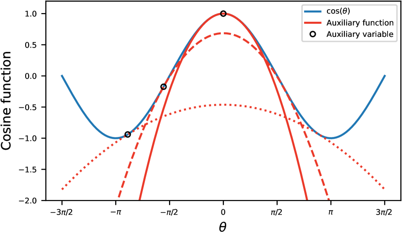
Figure 2: Example of the quadratic auxiliary function for the cosine function, where the point of tangency is the auxiliary variable $\theta_{k}$ at the $k$th frequency. Although other surrogate functions should exist, e.g., shown in [42], the proposed function is always the best for convergence, which requires only one update except for $\theta_{k}=\pm\pi$.

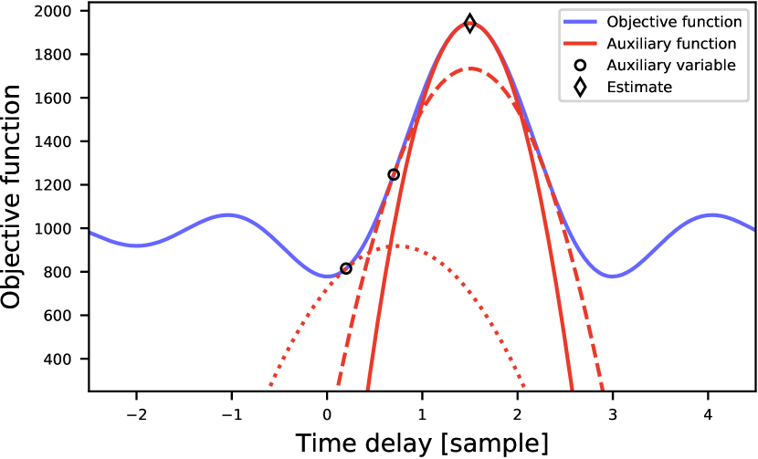
Figure 3: Examples of the objective function (24) and the auxiliary function (26). The objective function (24) is the CC function, which is a strictly unimodal function around the global maximum. Given an initial estimate picked from such a unimodal period, the proposed method must converge to the global optimal solution with monotonic increases in the objective function.

IV-D Derivation of Auxiliary Function and Update Rules

Since $Q_{s}(\tau,\bm{\theta})$ is a quadratic function, it is easily maximized with respect to $\tau$ by setting its derivative to zero:

$$\frac{\partial Q_{s}(\tau,\bm{\theta})}{\partial\tau}=-\sum_{k=0}^{T/2}A_{k}\omega_{k}\frac{\sin\theta_{k}}{\theta_{k}}(\omega_{k}\tau+\phi^{\prime}_{k})=0,$$ (29)

where $\phi^{\prime}_{k}=\phi_{k}+2\nu_{k}\pi$, Therefore, the maximizer is

$$\hat{\tau} =\frac{\sum_{k=0}^{T/2}A_{k}\omega_{k}^{2}(\sin\theta_{k}/\theta_{k})(-\phi^{\prime}_{k}/\omega_{k})}{\sum_{k=0}^{T/2}A_{k}\omega_{k}^{2}(\sin\theta_{k}/\theta_{k})}.$$ (30)

Now, under the condition of equality (27), we can substitute $\phi^{\prime}_{k}=\theta_{k}-\omega_{k}\tau$ for (30) and obtain the final update rules:

$$\nu_{k}^{(\ell)} \leftarrow\operatorname{round}\mathopen{}\mathclose{{}\left\{-\mathopen{}\mathclose{{}\left(\omega_{k}\tau^{(\ell)}+\phi_{k}}\right)/2\pi}\right\},$$ (31)

$$\theta_{k}^{(\ell)} \leftarrow\omega_{k}\tau^{(\ell)}+\phi_{k}+2\nu_{k}^{(\ell)}\pi,\quad k=0,\ldots,\frac{T}{2},$$ (32)

$$\tau^{(\ell+1)} \leftarrow\tau^{(\ell)}-\frac{\sum_{k=0}^{T/2}A_{k}\omega_{k}^{2}\mathopen{}\mathclose{{}\left(\sin\theta_{k}^{(\ell)}/\theta_{k}^{(\ell)}}\right)\frac{\theta_{k}^{(\ell)}}{\omega_{k}}}{\sum_{k=0}^{T/2}A_{k}\omega_{k}^{2}\mathopen{}\mathclose{{}\left(\sin\theta_{k}^{(\ell)}/\theta_{k}^{(\ell)}}\right)},$$ (33)

where $\operatorname{round}[\cdot]$ is a function that rounds the input to the nearest integer. Interestingly, the second term of (33) is a weighted sum of the auxiliary variables scaled by the normalized angular frequency, i.e., $\theta^{(\ell)}_{k}/\omega_{k}$, and $\theta^{(\ell)}_{k}/\omega_{k}$ corresponds to the candidate of the TD estimate at the frequency $k$.

V AuxTDE: Consistent time delay estimation

In this section, we propose AuxTDE, the method for estimating multiple sub-sample time delays simultaneously. This is the generalization of the method introduced in the previous section.

V-A Technical Approach for TDE

As we mentioned in section III, we aim to maximize the objective function (17) to obtain subsample TD estimates. To solve the joint optimization problem (16), we first consider to optimize $\bm{\tau}$ with fixed $\bm{a}_{k}$. Then, the denominator of (17) is constant that does not include $\bm{\tau}$. Now, the question is how to maximize the sum of numerator with respect to $\bm{\tau}$, which has the following structure:

$$\bm{g}_{{}k}^{\mathsf{H}}\mathopen{}\mathclose{{}\left(\bm{\tau}}\right)\bm{V}_{{}k}\,\bm{g}_{{}k}\mathopen{}\mathclose{{}\left(\bm{\tau}}\right)=\begin{pmatrix}a_{1k}e^{-\mathbbm{i}\omega_{k}\tau_{r1}}\\ a_{2k}e^{-\mathbbm{i}\omega_{k}\tau_{r2}}\\ \vdots\\[4.0pt] a_{Mk}e^{-\mathbbm{i}\omega_{k}\tau_{rM}}\end{pmatrix}^{\!\!\!\mathsf{H}}\bm{V}_{{}k}\begin{pmatrix}a_{1k}e^{-\mathbbm{i}\omega_{k}\tau_{r1}}\\ a_{2k}e^{-\mathbbm{i}\omega_{k}\tau_{r2}}\\ \vdots\\[4.0pt] a_{Mk}e^{-\mathbbm{i}\omega_{k}\tau_{rM}}\end{pmatrix},$$ (34)

where the parameters to be optimized are the exponent. Unfortunately, the maximization of the above function has no closed-form solution. Therefore, we consider applying the auxiliary function method as in section IV.

The objective function at the $k$th frequency (18) can be rewritten as a sum of the cosine function using the conjugate symmetry of $\bm{V}_{{}k}$ and Euler’s formula, the same as the derivation of (24),

$$\mathcal{J}_{{}k}\mathopen{}\mathclose{{}\left(\bm{\tau}}\right) =\sum_{i=1}^{M}\sum_{j=1}^{M}A_{ijk}\cos\mathopen{}\mathclose{{}\left(\omega_{{}k}\tau_{ij}+\phi_{ijk}}\right),$$ (35)

where $A_{ijk}=\beta_{k}a_{ik}a_{jk}|V_{ijk}|$, $\phi_{ijk}=\angle V_{ijk}$, and the denominator is omitted. It is worth noting that because the difference between two TDs, i.e., $\tau_{ij}=\tau_{rj}-\tau_{ri}$ in (35), is equal to $t_{j}-t_{i}$, the objective function is independent of the reference sensor $r$. Now, we propose the quadratic form auxiliary function for MCC, which has the closed-form solution. Here, we consider updating $\bm{\tau}$, $\bm{a}_{{}k}$, and $\sigma_{m}$ alternately.

V-B Quadratic Form Auxiliary Function for TDE

Similarly to subsection IV-B, we design the auxiliary function $Q(\bm{\tau},\bm{\theta})$ for multiple TDs $\bm{\tau}$ that satisfies the following properties:

• $\mathcal{J}\mathopen{}\mathclose{{}\left(\bm{\tau}}\right)\geq Q(\bm{\tau},\bm{\theta})$ for any $\bm{\tau}$ and $\bm{\theta}$,

• For any $\bm{\tau}$, $\exists\bm{\theta}=f(\bm{\tau})$ such that $\mathcal{J}(\bm{\tau})=Q(\bm{\tau},\bm{\theta})$,

where $\bm{\theta}=(\theta_{ijk})_{1\leq i,j\leq M,0\leq k\leq T/2}$ are auxiliary variables. Provided such a $Q(\bm{\tau},\bm{\theta})$ exists and given an initial estimate $\hat{\bm{\tau}}^{(0)}$, the following sequence of updates is guaranteed to converge to a local maximum:

$$\bm{\theta}^{(\ell)}=f(\hat{\bm{\tau}}^{(\ell)}),\quad\hat{\bm{\tau}}^{(\ell+1)}=\underset{\bm{\tau}\in\mathbb{R}}{\arg\max}\ Q(\hat{\bm{\tau}}^{(\ell)},\bm{\theta}^{(\ell)}).$$ (36)

We here propose an auxiliary function for $\mathcal{J}(\bm{\tau})$, i.e., $\mathcal{J}(\bm{\tau})\geq Q(\bm{\tau},\bm{\theta})$.

Theorem 2.

The following is an auxiliary function for $\mathcal{J}(\bm{\tau})$:

$$Q(\bm{\tau},\bm{\theta}) =\frac{1}{T}\sum_{k=0}^{T/2}Q_{{}k}(\bm{\tau},\bm{\theta}),$$ (37)

$$Q_{{}k}(\bm{\tau},\bm{\theta}) =\sum_{i=1}^{M}\sum_{j=1}^{M}\begin{aligned} \Biggl{\{}&-B_{ijk}\mathopen{}\mathclose{{}\left(\omega_{{}k}\tau_{ij}+\phi_{ijk}+2\nu_{ijk}\pi}\right)^{2}\\ &+\cos\theta_{ijk}+\frac{1}{2}\theta_{ijk}\sin\theta_{ijk}\Biggr{\}},\end{aligned}$$ (38)

$$B_{ijk} =\frac{A_{ijk}}{2}\frac{\sin\theta_{ijk}}{\theta_{ijk}},$$ (39)

where $\nu_{ijk}\in\mathbb{Z}$ is such that $|\omega_{{}k}\tau_{ij}+\phi_{ijk}+2\nu_{ijk}\pi|\leq\pi$. The auxiliary variables are $\theta_{ijk}$ and $\nu_{ijk}$ and $Q(\bm{\tau},\bm{\theta})=\mathcal{J}\mathopen{}\mathclose{{}\left(\bm{\tau}}\right)$ holds when

$$\theta_{ijk}=\omega_{{}k}\tau_{ij}+\phi_{ijk}+2\nu_{ijk}\pi,\ \forall i,j,k.$$ (40)

This theorem is a direct consequence of Proposition 1 with regards to a cosine function. The auxiliary function (38) can be rewritten as the vector quadratic form:

$$Q_{{}k}(\bm{\tau},\bm{\theta}) =-\bm{\tau}^{\mathsf{T}}\bm{C}_{{}k}\bm{\tau}-2\bm{c}_{{}k}^{\mathsf{T}}\bm{\tau}+{\rm Const.},$$ (41)

$$\bm{C}_{{}k} =\omega_{{}k}^{2}\mathopen{}\mathclose{{}\left\{\mathop{\rm diag}\mathopen{}\mathclose{{}\left(\bm{b}_{{}k}}\right)-\bm{B}_{{}k}}\right\},$$ (42)

$$\bm{b}_{{}k} =\mathopen{}\mathclose{{}\left(\sum_{i=1}^{M}B_{{i1}k},\ \dots,\ \sum_{i=1}^{M}B_{{iM}k}}\right)^{\!\!\!\mathsf{T}},$$ (43)

$$\bm{c}_{{}k} =\omega_{{}k}\mathopen{}\mathclose{{}\left(\sum_{i=1}^{M}B_{{i1}k}\phi^{\prime}_{{i1}k},\ \dots,\ \sum_{i=1}^{M}B_{{iM}k}\phi^{\prime}_{{iM}k}}\right)^{\!\!\!\mathsf{T}},$$ (44)

where $\bm{B}_{{}k}=(B_{ij})_{k,1\leq i,j\leq M}$ and $\phi^{\prime}_{ijk}=\phi_{ijk}+2\nu_{ijk}\pi$. $\bm{C}_{{}k}$ is the positive semidefinite matrix [47] and thus $-\bm{\tau}^{\mathsf{T}}\bm{C}_{{}k}\bm{\tau}$ is the convex upward function. We show an example of the objective function and auxiliary functions in Figs. 4LABEL:sub@subfig:mobj–LABEL:sub@subfig:maux3, where $M=3$ (that is, there are two TDs). The objective function, the MCC, is globally lower bounded by the proposed auxiliary function $Q(\bm{\tau},\bm{\theta})$ at any point and has exactly one point of tangency.

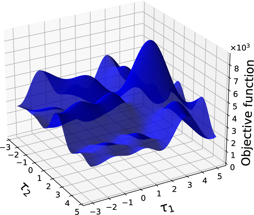
(a)

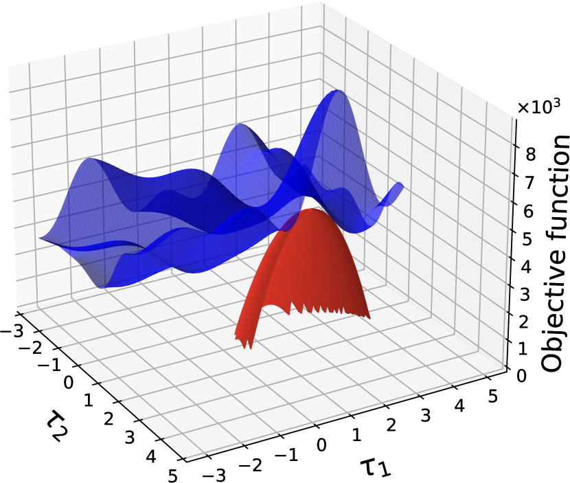
(b)

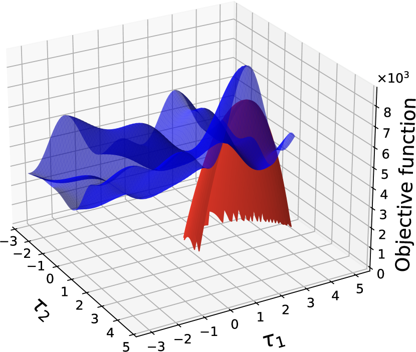
(c)

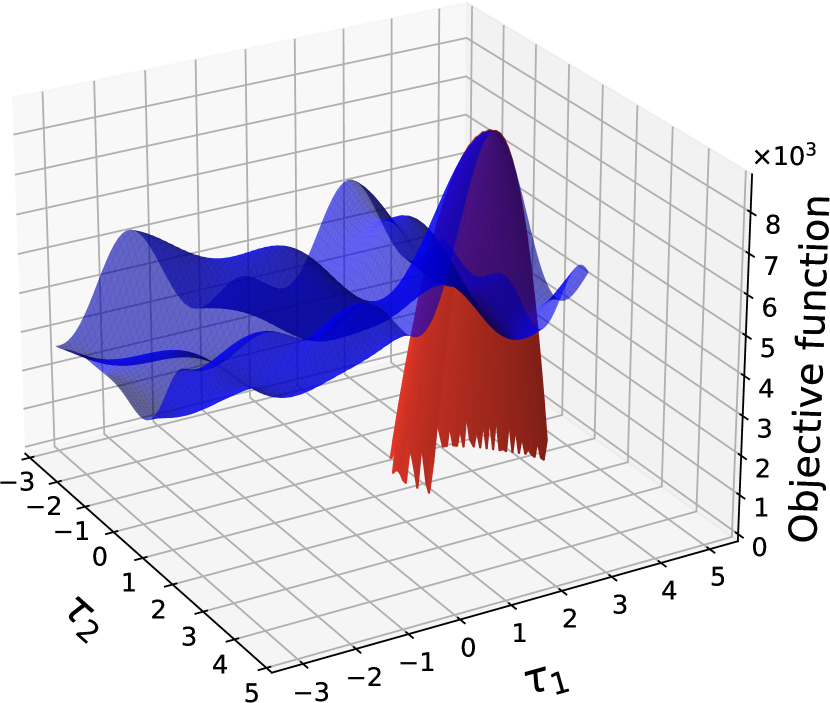
(d)

Figure 4: Examples of the objective function (blue) and auxiliary functions (red), where these functions are shown in only the range that takes a value more than $0$. (a) objective function only. (b)–(d) auxiliary functions, where the TD estimates are $(1.7,1.5)$, $(2,1.5)$, and $(3,1.5)$, respectively.

V-C Derivation of Auxiliary Function and Update Rules

To maximize the auxiliary function $Q(\bm{\tau},\bm{\theta})$ under the constraint of $\tau_{rr}=0$, we find the stationary point of the function $\sum_{k=0}^{T/2}Q_{{}k}(\bm{\tau},\bm{\theta})-\lambda\tau_{rr}$, where $\lambda$ is the Lagrange multiplier. Since $Q_{{}k}(\bm{\tau},\bm{\theta})$ is a quadratic form, it is easily maximized with respect to $\bm{\tau}$ by setting its derivative to zero:

$$\frac{\partial Q\mathopen{}\mathclose{{}\left(\bm{\tau},\bm{\theta}}\right)}{\partial\bm{\tau}^{\mathsf{T}}} =-\sum_{k=0}^{T/2}\mathopen{}\mathclose{{}\left\{2\bm{C}_{{}k}\bm{\tau}+2\bm{c}_{{}k}}\right\}-\lambda\bm{e}_{r}=0,$$ (45)

where $\bm{e}_{r}$ is a unit vector whose only $r$th element is $1$. Then, we obtain

$$\bar{\bm{\tau}} =-\mathopen{}\mathclose{{}\left(\sum_{k=0}^{T/2}\bar{\bm{C}}_{{}k}}\right)^{\raisebox{0.60275pt}{$\!\!\!\scriptscriptstyle-\!$}1}\sum_{k=0}^{T/2}\bar{\bm{c}}_{{}k},$$ (46)

where $\bar{\bm{C}}_{{}k}$ is an $M-1\times M-1$ matrix eliminating the $r$th row and column from $\bm{C}_{k}$, namely, $\bar{\bm{C}}_{{}k}=(C_{ij})_{k,1\leq i,j\leq M,i,j\neq r}$. Similarly, $\bar{\bm{\tau}}=(\tau_{ri})_{1\leq i\leq M,i\neq r}$ and $\bar{\bm{c}}_{{}k}=(c_{i})_{1\leq i\leq M,i\neq r}$.

Finally, under the condition of equality (40), we can substitute $\phi^{\prime}_{ijk}=\theta_{ijk}-\omega_{{}k}\tau_{ij}$ and obtain the update rules:

$$\nu^{(\ell)}_{ijk} \leftarrow\operatorname{round}\mathopen{}\mathclose{{}\left\{-\mathopen{}\mathclose{{}\left(\omega_{{}k}\tau_{ij}^{(\ell)}+\phi_{ijk}}\right)/2\pi}\right\},$$ (47)

$$\theta^{(\ell)}_{ijk} \leftarrow\omega_{{}k}\tau_{ij}^{(\ell)}+\phi_{ijk}+2\nu^{(\ell)}_{ijk}\pi,\ \forall i,j,k,$$ (48)

$$\bar{\bm{\tau}}^{(\ell+1)} \leftarrow\bar{\bm{\tau}}^{(\ell)}-\mathopen{}\mathclose{{}\left(\sum_{k=0}^{T/2}\bar{\bm{C}}^{(\ell)}_{{}k}}\right)^{\raisebox{0.60275pt}{$\!\!\!\scriptscriptstyle-\!$}1}\sum_{k=0}^{T/2}\bar{\bm{c}}^{\prime(\ell)}_{{}k},$$ (49)

where $\bar{\bm{c}}^{\prime}_{{}k}=(c^{\prime}_{j})_{k,1\leq j\leq M,j\neq{r}}$ and

$$c^{\prime}_{jk}=\omega_{{}k}\sum_{i=1}^{M}B_{ijk}\frac{\theta_{ijk}}{\omega_{{}k}}.$$ (50)

Note that the above update rules are in complete agreement with those in the case of two sensors (31)–(33), and hence the TD estimate is also identity.

V-D Amplitude Estimation

Although our purpose is to estimate subsample TDs, we need to also estimate the unknown parameter $\bm{a}_{k}$. One of the solutions is the use of fixed amplitudes $\bm{a}_{k}=\bm{1}$ for all $k$. However, we here propose the following method for estimating $\bm{a}_{k}$, which may result in improved TD estimates.

First, we arrange the numerator of $\mathcal{J}_{{}k}\mathopen{}\mathclose{{}\left(\bm{a}_{{}k},\bm{\tau}}\right)$ as

$$\bm{g}_{{}k}^{\mathsf{H}}\mathopen{}\mathclose{{}\left(\bm{a}_{{}k},\bm{\tau}}\right)\bm{V}_{{}k}\,\bm{g}_{{}k}\mathopen{}\mathclose{{}\left(\bm{a}_{{}k},\bm{\tau}}\right) =\bm{a}_{{}k}^{\mathsf{T}}\bm{V}_{{}k}^{\prime}\mathopen{}\mathclose{{}\left(\bm{\tau}}\right)\,\bm{a}_{{}k},$$ (51)

$$\bm{V}_{{}k}^{\prime}\mathopen{}\mathclose{{}\left(\bm{\tau}}\right) =\bm{V}_{{}k}\odot\bm{P}_{{}k}\mathopen{}\mathclose{{}\left(\bm{\tau}}\right),$$ (52)

$$\bm{P}_{{}k}\mathopen{}\mathclose{{}\left(\bm{\tau}}\right) =\bm{p}_{{}k}\mathopen{}\mathclose{{}\left(\bm{\tau}}\right)\bm{p}_{{}k}^{\mathsf{H}}\mathopen{}\mathclose{{}\left(\bm{\tau}}\right),$$ (53)

$$\bm{p}_{{}k}\mathopen{}\mathclose{{}\left(\bm{\tau}}\right) =\mathopen{}\mathclose{{}\left[{e^{\mathbbm{i}\omega_{{}k}\tau_{r1}}}\ \cdots\ {e^{\mathbbm{i}\omega_{{}k}\tau_{rM}}}}\right]^{\mathsf{T}},$$ (54)

where $\bm{V}^{\prime}_{{}k}\mathopen{}\mathclose{{}\left(\bm{\tau}}\right)$ is an Hermitian matrix and $\bm{P}_{{}k}\mathopen{}\mathclose{{}\left(\bm{\tau}}\right)$ is an $M\times M$ matrix. At fixed $\bm{\tau}$, the optimization problem (16) becomes

$$\operatorname*{arg~{}max}_{\bm{a}_{{}k}}\ \frac{1}{T}\sum_{k=0}^{T/2}\beta_{{}k}\mathcal{J}_{{}k}(\bm{a}_{{}k})\ \ \mathrm{s.t.}\ \ a_{mk}\geq 0\ \ \forall m,k,$$ (55)

$$\mathcal{J}_{{}k}(\bm{a}_{{}k})=\frac{\bm{a}_{{}k}^{\mathsf{T}}\bm{V}^{\prime}_{{}k}\bm{a}_{{}k}}{\bm{a}_{{}k}^{\mathsf{T}}\bm{a}_{{}k}}=\frac{\bm{a}_{{}k}^{\mathsf{T}}\Re[\bm{V}^{\prime}_{{}k}]\bm{a}_{{}k}}{\bm{a}_{{}k}^{\mathsf{T}}\bm{a}_{{}k}},$$ (56)

where $\Re[\cdot]$ takes the real part of the input argument, and again $\beta_{0}=\beta_{T/2}=1$ and $\beta_{k}=2$ for $k\not\in\{0,T/2\}$. The objective function (56) is known as the Rayleigh quotient, where $\bm{a}_{k}$ is the non-zero (and also non-negative in our problem) vector. Hence, the optimization problem is the maximization of the Rayleigh quotient with a non-negative constraint, which may be of general interest.

V-D1 Unconstrained case

The solution of this maximization problem without any constraint is given by the eigenvalue decomposition (e.g., [42]). Since the objective function (56) is invariant to the scale of the amplitudes, we optimize $\bm{a}_{{}k}$ under the constraint $\|\bm{a}_{{}k}\|_{2}^{2}=1$ and compensate for $a_{rk}$ to $1$ at the end of update sequences. Then, using the method of Lagrange multipliers, we find the stationary point by taking the gradient with respect to $\bm{a}_{{}k}$ and setting it to zero as

$$\frac{\partial\mathcal{J}_{{}k}(\bm{a}_{{}k})}{\partial\bm{a}_{{}k}}=\bm{V}^{\prime}_{{}k}\bm{a}_{{}k}-\lambda_{{}k}\bm{a}_{{}k} =\bm{0},$$ (57)

where $\lambda_{{}k}$ is the $k$th Lagrange multiplier.

This result is well known as the eigenvalue problem. Although any eigenvector of $\bm{V}_{{}k}^{\prime}$ used as $\bm{a}_{{}k}$ satisfies (57), we choose the eigenvector corresponding to the largest eigenvalue (hereafter, we simply denote it as the largest eigenvector) for maximizing the objective function (56).

V-D2 Constrained case

One solution for the maximization of the Rayleigh quotient with non-negative constraint is the projection. Since the largest eigenvector can take a negative value, we project its elements $\hat{a}_{mk}$ to the positive domain

$$\hat{a}_{mk}\leftarrow\max(\hat{a}_{mk},\ 0)\ \ \forall m$$ (58)

to satisfy the non-negative constraint.

Although the largest eigenvector is absolutely the solution of (56), there is no guarantee that the projected eigenvector maximizes the objective function. We thus propose the alternative method based on the auxiliary function method.

Theorem 3.

Let $\|\bm{a}_{{}k}\|_{2}^{2}=1$ for all $k$. The following is an auxiliary function for the Rayleigh quotient $\mathcal{J}_{{}k}(\bm{a}_{{}k})$ [42],

$$Q^{a}_{{}k}(\bm{a}_{{}k},\bm{\theta}) =2\bm{\theta}_{{}k}\bm{V}_{{}k}^{\prime}\bm{a}_{{}k}-\bm{\theta}_{{}k}\bm{V}^{\prime}_{{}k}\bm{\theta}_{{}k},$$ (59)

where $\bm{\theta}=\mathopen{}\mathclose{{}\left[{\bm{\theta}_{0}}\ \cdots\ {\bm{\theta}_{T/2}}}\right]^{\mathsf{T}}$ are auxiliary variables and $Q^{a}_{{}k}(\bm{a}_{{}k},\bm{\theta})=\mathcal{J}_{{}k}(\bm{a}_{{}k})$ holds when

$$\bm{\theta}_{{}k}=\bm{a}_{{}k}.$$ (60)

The auxiliary function (59) is the linear form of the vector $\bm{a}_{{}k}$ and is easily maximized even under the non-negative constraint. Then, the update rules are

$$\bm{a}_{{}k}^{(\ell+1)} \leftarrow\bm{V}_{{}k}^{\prime}\bm{a}_{{}k}^{(\ell)},$$ (61)

$$a_{mk}^{(\ell+1)} \leftarrow\max\mathopen{}\mathclose{{}\left(a_{mk}^{(\ell+1)},\ 0}\right)\ \ \forall m,$$ (62)

$$\bm{a}_{{}k}^{(\ell+1)} \leftarrow\bm{a}_{{}k}^{(\ell+1)}/\|\bm{a}_{{}k}^{(\ell+1)}\|_{2}^{2}.$$ (63)

These update sequences are guaranteed to converge to a local maximum, whereas the projected largest eigenvector (58) does not attain it unless all elements are positive without projection.

Interestingly, there is a well-known algorithm, namely, the power method (power iteration), for estimating the largest eigenvector. The power method iteratively updates the eigenvector estimate in (61) and (63). The above algorithm shows that we can obtain the local maximum in the same scheme even under the non-negative constraint by applying the projection to the positive domain (62).

V-D3 Shared amplitude case

We can consider the observation model with a shared amplitude vector for all frequencies, that is, $\bm{a}_{{}k}$ is identical for all $k$. The amplitude estimation with this alternative model can be easily realized by using averaged $\bm{V}_{{}k}^{\prime}$:

$$\bm{V}^{\prime}_{{\rm mean}}=\frac{1}{T/2+1}\sum_{k=0}^{T/2}\bm{V}_{{}k}^{\prime},$$ (64)

in update sequences (61)–(63). We expect that this alternative model is robust against the estimation error in amplitudes and measurement environments.

V-E Update of Noise Variances

To compute the observations and RTF weighted by the standard deviation $\sigma_{m}$ defined in (12) and (13), respectively, we finally update the variance $\bm{\Sigma}$ of the complex multivariate Gaussian distribution $\mathcal{N}_{c}\mathopen{}\mathclose{{}\left(\bm{\mu},\bm{\Sigma}}\right)$ as follows:

$$\sigma_{m}^{2}\leftarrow\frac{1}{NT}\sum_{k=0}^{T/2}\sum_{n=0}^{N-1}\beta_{k}|x_{{m}kn}-\hat{\mbox{\large$s$}}_{{}kn}g_{mk}\mathopen{}\mathclose{{}\left(a_{mk},\tau_{rm}}\right)|^{2},$$ (65)

where $g_{mk}\mathopen{}\mathclose{{}\left(a_{mk},\tau_{rm}}\right)=a_{mk}e^{-\mathbbm{i}\omega_{k}\tau_{rm}}$ and $\hat{\mbox{\large$s$}}_{{}kn}$ is computed by (11).

V-F Algorithm of AuxTDE

Finally, we summarize the update sequences of the AuxTDE in Algorithm 1, where three types of iteration exist, for the update of $\bm{\tau}$, $\bm{a}_{{}k}$, and their alternate updates indexed by $\ell_{\tau}$, $\ell_{a}$ and $\ell_{e}$, respectively. The maximum iterations $L_{\tau}$, $L_{a}$, and $L_{e}$ can be $1$. The initialization of $\bm{\tau}$ can be performed by the pairwise method. For instance, the discrete maximum (GCC method [22]) and the result of parabolic interpolation [28] can be used. Basically, better initial estimates lead to faster convergence, and parabolic interpolation is thus better in practice.

Algorithm 1 AuxTDE

$\bm{x}_{{}kn}$

$\bm{\tau}$

Initialize:

      Initialize $\bm{\tau}$ Initialize $\bm{a}_{{}k}=1$ for all $k$ Initialize $\sigma_{m}^{2}=1$ for all $m$ Compute $\phi_{ijk}$ and $A_{ijk}$ for all $i,j,k$ from $\bm{V}_{{}k}$

for $\ell_{e}=0,1,\dots,L_{e}-1$ do

     $A^{\prime}_{ijk}\leftarrow A_{ijk}/\sigma_{i}\sigma_{j}$ $\triangleright$ corresponds to (12)

     for $\ell_{\tau}=0,1,\dots,L_{\tau}-1$ do

         $\bm{\tau}\leftarrow{\tt update\_td}(\bm{a}_{{}k},\bm{\tau},A^{\prime}_{ijk},\phi_{ijk})$

     end for

     for $\ell_{a}=0,1,\dots,L_{a}-1$ do

         $\bm{a}_{{}k}\leftarrow{\tt update\_amp}(\bm{a}_{{}k},\bm{\tau},A^{\prime}_{ijk},\phi_{ijk})$ for all $k$

     end for

     Update $\sigma_{m}^{2}$ by (65)

end for

Function ${\tt update\_td}$($\bm{a}_{{}k}$, $\bm{\tau}$, $A_{ijk}$, $\phi_{ijk}$)

      Update $\bm{\theta}$ by (47) and (48) Compute $\bm{C}_{{}k}$ and $\bm{c}_{{}k}$ by (42)–(44) Update $\bm{\tau}$ by (49) return $\bm{\tau}$

end Function

Function ${\tt update\_amp}$($\bm{a}_{{}k}$, $\bm{\tau}$, $A_{ijk}$, $\phi_{ijk}$)

     

Compute $V_{{}k}^{\prime}$ by (52)–(54)

Update $\bm{a}_{{}k}$ by (61)–(63)

return $\bm{a}_{{}k}$

end Function

VI Experimental Analysis of the AuxTDE algorithm

VI-A Empirical Convergence to the Local Maximum

First, we confirm the convergence of the AuxTDE by depicting the objective function, where we simulated $M=2$ observations whose sub-sample TD was set to $2.0996$ samples. We used English female speech as a target signal sampled at $16\text{\,}\mathrm{kHz}$ and added white Gaussian noise to each microphone with signal-to-noise ratio (SNR) of $10\text{\,}\mathrm{dB}$. Fig. 5 shows the convergence of the objective function (17) with the AuxTDE for different initial values. We set the initial value of the proposed method to every three samples from $2$ to $29$. In accordance with this figure, we can confirm that the proposed method will converge to the global maximum if an appropriate initial value is given. Moreover, this figure shows the guaranteed monotonic increase in the objective function for any initial value. The initial value must be picked from the unimodal period, including the global maximum, to reach it, where the range is between $-20$ to $22$ samples in this figure. Basically, the conventional GCC method is a good way to obtain such an initial estimate. Even when the initial estimate is outside the appropriate range, the convergence to the local maximum is always guaranteed owing to the characteristic of the auxiliary function method. Additionally, the better the initial estimate is (e.g., in the case of using the parabolic interpolation), the faster the convergence is.

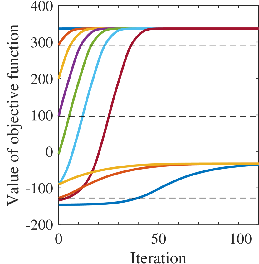
Figure 5: Left: the value of objective function via the proposed method over initial values, where $M=2$. Different curves represent different values of the initial TD estimate, taken every three samples from $2$ to $29$. Right: objective function.

VI-B Empirical Convergence and Consistent TD Estimates

As we mentioned in section II-C, the AuxTDE attains consistent TD estimates owing to the observation model. Although we must set the reference sensor for computing TDs since these are relative values, the AuxTDE can obtain the same TD estimates regardless of the reference sensor. This property can be confirmed by verifying the objective function. Here, we used pyroomacoustics [48] to simulate a reverberant environment and generated eight microphone signals with a target source, as shown in Fig. 6. In this experiment, we focused on the TDE algorithm of the AuxTDE and fixed the amplitude $\bm{a}_{k}$ and the variance $\sigma^{2}_{m}$ to $1$ for all elements. We set initial values of $\bm{\tau}$ as the estimates by the pairwise method using the parabolic interpolation [28] of the GCC method [22] whose weights were one for all frequencies. For the pairwise method, there were eight choices of the reference microphone $r$; thus, we computed the same number of the TD estimate vector $\hat{\bm{\tau}}_{r}$. Then, we computed the objective function of the AuxTDE (17) with every $\hat{\bm{\tau}}_{r}$ and showed them in Fig. 7 at the $0$th iteration.

The objective function values at the $0$th iteration in Fig. 7 show the dependence of the pairwise GCC method on the reference microphone $r$. This result implies that the performance of TD estimation also varied. Interestingly, the best performance in terms of the objective function was achieved with $r=3$, whereas the worst one was achieved with $r=4$ (see Fig. 6). It is difficult to predict the best reference microphone in advance, even when the actual layout of the source and microphones was known. Moreover, since we cannot obtain true TD values in practice, the evaluation criterion for the pairwise method is also unclear.

In contrast, the AuxTDE with these initial estimates monotonically increased the objective function and converged to the same local maximum regardless of the reference microphone, as shown in Fig. 7. This result indicates that consistent TDs were obtained owing to the joint optimization (16) and the transfer system model (3). Additionally, it can be said that these results are the best in terms of ML. Similar to the result in subsection VI-A, the better initial estimate led to faster convergence.

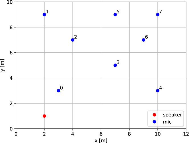
Figure 6: Example of the microphones and target source alignment. The numbers near the microphones denote their indices.

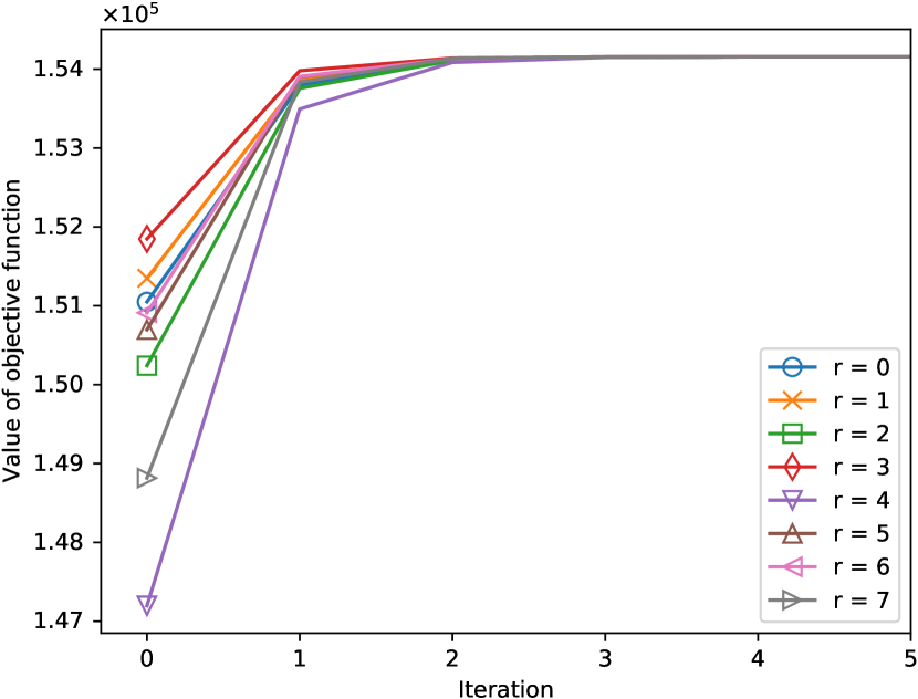
Figure 7: Objective function and convergence via the iterative updates of the AuxTDE. The $0$th iteration corresponds to the objective function using the initial value $\bm{\tau}^{(0)}$ estimated by the pairwise GCC method with parabolic interpolation. Different curves correspond to the different reference microphones specified by $r$.

VII Experiments of Time Delay Estimation

VII-A Experimental Condition

In this section, we evaluated the performance of TD estimation. We used the pyroomacoustics [48] to simulate reverberant room environments. We synthesized $M$ observed signals sampled at $16\text{\,}\mathrm{kHz}$ with simulated room impulse responses with a reverberation time of approximately $200\text{\,}\mathrm{ms}$. The target signal of $5\text{\,}\mathrm{s}$ was randomly generated following normal Gaussian distribution and was contaminated by additive Gaussian noise, where SNR was set to $20\text{\,}\mathrm{dB}$. The target source and microphones are randomly located in a room of $3\text{\,}\mathrm{m}$ $\times$ $4\text{\,}\mathrm{m}$ $\times$ $3\text{\,}\mathrm{m}$ size, as in the example shown in Fig. 6. We tested three types of microphone alignment: widely placed $M=4$ and $M=8$ microphones assuming distributed microphone arrays, where they are located at least $0.2\text{\,}\mathrm{m}$ away from each other, and closely placed $M=8$ microphones assuming an ordinary microphone array. Note that we assumed that all microphones are synchronized, and no sampling frequency mismatch problem [20] occurred. We performed STFT with a rectangle window for the observed signals, where the window length is $4096$ samples, and each frame is half-overlapped.

We evaluated three types of AuxTDE algorithm for amplitude estimation: the original AuxTDE, denoted as AuxTDE_freqAmp, estimates both TDs and frequency-dependent amplitudes simultaneously as shown in Algorithm 1, AuxTDE_shrdAmp estimates shared (frequency-independent) amplitude by the algorithm described in subsection V-D3, and AuxTDE_unitAmp estimates only TDs with fixed amplitudes ($\bm{a}_{k}=\bm{1}\ \forall k$). The number of iterations of each method is listed in Table I, and all the methods update the variances.

For comparison, we evaluated three types of pairwise methods: the GCC method [22] (PW-GCC), the GCC method with parabolic interpolation [28] (PW-Parafit), and the GCC method with the AuxTDE for two channels (PW-AuxTDE). Although the AuxTDE is applicable with three or more microphones, we used it here as the pairwise method merely for comparison. We used every microphone as the reference one for all the methods and obtained $M$ TD estimate vectors $\hat{\bm{\tau}}_{r}$.

For the evaluation criterion, we used root mean square errors between the estimated TDs $\hat{\bm{\tau}}_{r,p}$ and computed ones $\bm{\tau}^{\star}_{r,p}$ defined as

$${\rm RMSE}=\sqrt{\frac{1}{PM(M-1)}\sum_{p=1}^{P}\sum_{r=1}^{M}\|\hat{\bm{\tau}}_{r,p}-\bm{\tau}^{\star}_{r,p}\|^{2}_{2}},$$ (66)

where $P$ denotes the number of simulations, and the subscript $p$ denotes the simulation index. $P$ was $1200$ in this experiment. Since the true TDs were unknown, we computed the TDs from the distance between the target source and each microphone and used it as the ground truth instead, where the speed of sound was $343\text{\,}\mathrm{m}\mathrm{/}\mathrm{s}$ (pyroomacoustics default). Note that we eliminated several gross error cases from the evaluation. The occurrence of gross errors depended on the conditions (e.g., microphone positions and initial estimates) and was approximately $0.1\text{\,}\mathrm{\char 37\relax}$ in this experiment.

In addition to the evaluation of RMSE, we evaluate how inconsistent the TD estimates are. On the basis of Definition 1 for the consistent TDs, we define the mean absolute inconsistent delay (MID) as follows:

$$\mathrm{MID}=\mathopen{}\mathclose{{}\left(\frac{1}{M-1}}\right)^{\!\!2}\sum_{r^{\prime}=1}^{M}\sum_{m=1}^{M}\bigl{[}\mathopen{}\mathclose{{}\left|\tau_{r^{\prime}m}-\mathopen{}\mathclose{{}\left(\tau_{r^{\prime}r}+\tau_{rm}}\right)}\right|\bigr{]},$$ (67)

where $r=1$ in this experiment. Clearly, MID is $0$ if the TD estimates are completely consistent; otherwise, it takes a high value. To evaluate the MID, we thus need to perform TD estimation $M$ times in total by setting each sensor as the reference one.

TABLE I: Number of iterations of each AuxTDE variant.

Method	$\ell_{\tau}$	$\ell_{a}$	$\ell_{e}$
AuxTDE_freqAmp	10	10	3
AuxTDE_unitAmp	10	-	3
AuxTDE_shrdAmp	10	10	3

TABLE II: RMSEs between the estimated and ground truth TDs for each method and environment.

Method	# of microphones $M$
	4 (DMA)	8 (DMA)	8 (Array)
PW-GCC	$28.8\times 10^{-2}$	$28.9\times 10^{-2}$	$28.8\times 10^{-2}$
PW-Parafit	$8.45\times 10^{-2}$	$8.44\times 10^{-2}$	$8.56\times 10^{-2}$
PW-AuxTDE	$1.40\times 10^{-2}$	$1.38\times 10^{-2}$	$2.21\times 10^{-2}$
AuxTDE_unitAmp	$1.07\times 10^{-2}$	$0.826\times 10^{-2}$	$\mathbf{1.37\times 10^{-2}}$
AuxTDE_freqAmp	$1.14\times 10^{-2}$	$0.856\times 10^{-2}$	$1.48\times 10^{-2}$
AuxTDE_shrdAmp	$\mathbf{1.06\times 10^{-2}}$	$\mathbf{0.817\times 10^{-2}}$	$1.39\times 10^{-2}$

TABLE III: MIDs for each method and environment.

Method	# of microphones $M$
	4 (DMA)	8 (DMA)	8 (Array)
PW-GCC	$16.5\times 10^{-2}$	$21.7\times 10^{-2}$	$21.4\times 10^{-2}$
PW-parafit	$6.68\times 10^{-2}$	$8.71\times 10^{-2}$	$8.83\times 10^{-2}$
PW-AuxTDE	$1.09\times 10^{-2}$	$1.40\times 10^{-2}$	$2.22\times 10^{-2}$
AuxTDE_unitAmp	$3.88\times 10^{-12}$	$3.88\times 10^{-12}$	$3.73\times 10^{-12}$
AuxTDE_freqAmp	$2.85\times 10^{-12}$	$0.941\times 10^{-12}$	$7.79\times 10^{-12}$
AuxTDE_shrdAmp	$0.162\times 10^{-12}$	$0.122\times 10^{-12}$	$0.290\times 10^{-12}$

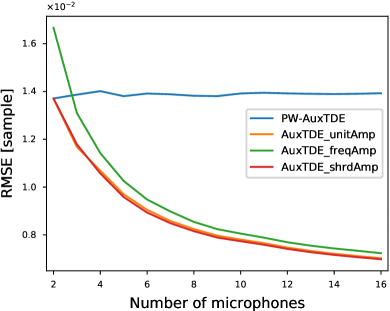
(a)

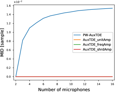
(b)

Figure 8: (a) Accuracy of TD estimation and (b) MIDs in TDE as functions of the number of microphones $M$, where $M$ varies in the range of $2$ to $16$. The MIDs of AuxTDE algorithms except for PW-AuxTDE varied from $10^{-12}$ to $10^{-13}$. The proposed methods benefited from using more microphones, while the pairwise method did not.

VII-B Results and Discussion

Table II shows the RMSEs, the results of TDs estimation. The theoretical error in PW-GCC is $0.25$, and values close to this error were obtained. PW-Parafit significantly improved the estimation accuracy with quite low computational cost, and PW-AuxTDE attained greater improvement with the efficient iterative algorithm. Their RMSEs were almost the same for all the microphone alignments.

The RMSEs of AuxTDE algorithms except for PW-AuxTDE were superior to that of the pairwise methods in every case. Additionally, the performance was improved by using eight microphones than four microphones. Since our model includes spatial information contained in the entire observation, AuxTDE could utilize the consistency in TD parameters. Furthermore, the performance with DMAs was relatively higher than in the case of using an array of closely placed microphones in this experiment. This result implies that one of the suitable applications of the AuxTDE is a DMA (and other distributed sensor systems), which consists of widely placed sensors and has broad spatial information.

The simultaneous estimation of the amplitude (AuxTDE_freqAmp) degraded the performance in most cases compared with AuxTDE_unitAmp even though the performance of AuxTDE_freqAmp was superior to that of the pairwise methods. As one reason, we can consider that the constant amplitude used in AuxTDE_unitAmp (i.e., $\bm{a}_{{}k}=\bm{1}$ for all $k$) was an excellent a priori for TD estimation. Moreover, it is possible that estimating frequency-dependent amplitudes overfitted the acoustic environment. Estimating shared amplitudes (AuxTDE_shrdAmp) may be the better solution for some situations such as when using DMA. For example, when the gain of each sensor differs, the mechanism of AuxTDE_shrdAmp may be able to reduce the negative effect due to their gain differences.

Table III shows the MID of the TD estimates. The MIDs of the pairwise methods were considerably high, and the order of MIDs was the same as the RMSEs (see also Table II). This means that the TD estimates were inconsistent. Therefore, there should be one best microphone that should be used as the reference microphone; however, the method to find it is unclear. On the other hand, the proposed methods that estimate all TDs simultaneously showed markedly low MIDs regardless of the microphone alignment. This means that the TD estimates were independent of the reference microphone. From the above, we can confirm the effectiveness of the proposed AuxTDE for TD estimation.

VII-C TD Estimation with a Number of Microphones

Finally, we investigated the relationship between the accuracy in TDE and the number of microphones to compare the proposed methods and the pairwise methods further. Experimental conditions are identical to those described in subsection VII-A except for the number of microphones $M$. It varies from $2$ to $16$, and they are located at least $0.2\text{\,}\mathrm{m}$ away from each other, assuming DMAs.

Figs. 8LABEL:sub@subfig:rmse and LABEL:sub@subfig:ic show the RMSE and MID of each method as functions of the number of microphones, respectively. Note that the results of PW-GCC and PW-Parafit are omitted because their performance changes with respect to $M$ tended to be the same as that of PW-AuxTDE. The TD estimates of each method except for AuxTDE_freqAmp are theoretically identical when $M=2$.

From Fig. 8LABEL:sub@subfig:rmse, the RMSE of PW-AuxTDE was independent of the number of microphones $M$. Since the pairwise method only uses partial spatial cue between two selected sensors, there are no benefits of increasing the number of sensors. In contrast, the MID increased (i.e., worsened) with increasing $M$, as shown in Fig. 8LABEL:sub@subfig:ic. The MID is theoretically zero when $M=2$ since the interchange of the reference sensor corresponds to the time reversal of the CC function. The choices of reference sensors increased with increasing $M$, and as a result, the MID became high.

In contrast to the above results, AuxTDE algorithms except for PW-AuxTDE improved the performance of TDE with increasing number of microphones. This result demonstrated the importance and efficacy of using entire spatial information captured by the microphones and consistent constraint for TDs. Additionally, the MIDs were considerably low (approximately $10^{-12}$); in other words, the TDs estimated by the proposed methods were consistent regardless of $M$. Finally, we concluded that AuxTDE algorithms are effective for TDE, which attains highly accurate and consistent TD estimates.

VIII Conclusions

In this paper, we proposed AuxTDE, a novel method for TD estimation, using the auxiliary function method. The joint optimization problem for consistent TDs and amplitudes was considered on the basis of ML estimation. The objective function, MCC function, encodes the CC function of all sensor pairs, which can thus be considered as the multidimensional extension of the CC function. The MCC, which is the nonconvex function, was lower-bounded by the quadratic auxiliary function, and efficient update rules that iteratively maximize the MCC were derived. In experiments, we demonstrated important properties of AuxTDE: monotonic increases in the objective function, convergence to the local maximum, and independence against the reference sensor. Additionally, we confirmed the efficacy of the AuxTDE through the experiment of TD estimation, where the AuxTDE attained highly accurate and consistent TD estimates. The future work includes the online extension of the AuxTDE and the heuristic extension of its algorithm.

Appendix A Proof of Proposition 1 and Theorems 1 and 2

A-A Proof of Proposition 1

Proof: Let

$$f(\theta)=\cos\theta+\frac{1}{2}\frac{\sin\theta_{0}}{\theta_{0}}\theta^{2}-\mathopen{}\mathclose{{}\left(\cos\theta_{0}+\frac{1}{2}\theta_{0}\sin\theta_{0}}\right).$$ (68)

Then, we have

$$f^{\prime}(\theta) =-\sin\theta+\frac{\sin\theta_{0}}{\theta_{0}}\theta=-\theta\mathopen{}\mathclose{{}\left(\frac{\sin\theta}{\theta}-\frac{\sin\theta_{0}}{\theta_{0}}}\right).$$ (69)

We separately consider the following three cases.

Case 1: $0<|\theta_{0}|<\pi$
Because $\sin\theta/\theta$ is monotonically decreasing in $0\leq\theta\leq\pi$,

$$f^{\prime}(\theta)\mathopen{}\mathclose{{}\left\{\begin{array}[]{cl}<0&(0\leq\theta<|\theta_{0}|),\\ =0&(\theta=|\theta_{0}|),\\ >0&(|\theta_{0}|<\theta\leq\pi).\end{array}}\right.$$ (73)

It thus appears that $f(\theta)$ attains its minimum at $|\theta_{0}|$. Moreover, $f(\theta_{0})=0$ and thus $f(\theta)\geq 0$ in $0\leq\theta\leq\pi$. Since $f(\theta)$ is an even function, its minimum value in $-\pi\leq\theta\leq\pi$ is also $0$. Because $\cos\theta$ is periodic but $-\theta^{2}$ is not, $f(\theta+2\nu\pi)>f(\theta)$ for any $-\pi\leq\theta\leq\pi$ and integer $\nu\neq 0$. Therefore, $f(\theta)\geq 0$, with equality if and only if $|\theta|=|\theta_{0}|$.

Case 2: $\theta_{0}=0$
In this case, for $0\leq\theta\leq\pi$, we have

$$f^{\prime}(\theta)\mathopen{}\mathclose{{}\left\{\begin{array}[]{cl}=0&(\theta=|\theta_{0}|=0)\\ >0&(|\theta_{0}|<\theta\leq\pi)\end{array}}\right.,$$ (76)

which means $f(\theta)$ takes a minimum value at $f(0)=0$ in $-\pi\leq\theta\leq\pi$. Similarly to case $1$, we obtain $f(\theta)\geq 0$, with equality if and only if $\theta=0$.

Case 3: $\theta_{0}=\pi$ or $\theta_{0}=-\pi$
In this case, $f(\theta)=\cos\theta+1$. Therefore $f(\theta)\geq 0$, with equality if and only if $\theta=(2\nu+1)\pi$ for any $\nu\in\mathbb{Z}$.   

A-B Proof of Theorems 1 and 2

Proof: Because $\cos(\omega_{k}\tau_{ij}+\phi_{ijk})=\cos(\omega_{k}\tau_{ij}+\phi_{ijk}+2\nu_{ijk}\pi)$ with $\nu_{ijk}\in\mathbb{Z}$, and because $\beta_{k}a_{ik}a_{jk}A_{ijk}\geq 0$, we can apply Proposition 1 separately to each term of the sum in (24) and (35).   

Appendix B Properties of matrices in subsection V-D

$\bm{P}_{{}k}$ is a positive semidefinite matrix because the following is satisfied for any complex-valued vector $\bm{z}$:

$$\bm{z}^{\mathsf{H}}\bm{P}_{{}k}\bm{z}=|\bm{p}_{{}k}^{\mathsf{H}}\bm{z}|^{2}\geq 0.$$ (77)

In accordance with the Schur product theorem, $\bm{V}_{{}k}^{\prime}$, which is the Hadamard product of two positive semidefinite matrices, is also the positive semidefinite matrix. Additionally, $\operatorname{rank}(\bm{P}_{{}k})=1$ and thus $\operatorname{rank}(\bm{V}_{{}k}^{\prime})=\operatorname{rank}(\bm{V}_{{}k})$. When we assume that the signal $s_{{}kn}$ and noises $\bm{u}_{{}kn}$ are uncorrelated, the covariance matrix $\bm{V}_{{}k}$ can be divided into the signal and noise parts as

$$\bm{V}_{{}k} =\operatorname*{\mathbb{E}}\mathopen{}\mathclose{{}\left[\bm{x}_{{}kn}\bm{x}^{\mathsf{H}}_{{}kn}}\right]=|s_{{}kn}|^{2}\bm{g}_{{}k}\bm{g}_{{}k}^{\mathsf{H}}+\operatorname*{\mathbb{E}}[\bm{u}_{{}kn}\bm{u}_{{}kn}^{\mathsf{H}}].$$ (78)

Following the subadditivity of the rank of the matrix, $\operatorname{rank}(\bm{V}_{{}k}^{\prime})\leq\operatorname{rank}(\operatorname*{\mathbb{E}}[\bm{u}_{{}kn}\bm{u}_{{}kn}^{\mathsf{H}}])+1$, where $\bm{g}_{{}k}\bm{g}_{{}k}^{\mathsf{H}}$ is a rank-$1$ matrix.

References

- [1] J. Chen, J. Benesty, and Y. Huang, “Time delay estimation in room acoustic environments: An overview,” EURASIP J. Adv. Signal Process., vol. 2006, pp. 1–19, Dec. 2006.
- [2] M. Brandstein, J. Adcock, and H. Silverman, “A closed-form location estimator for use with room environment microphone arrays,” IEEE Trans. Speech Audio Process., vol. 5, no. 1, pp. 45–50, 1997.
- [3] T. Gustafsson, B. Rao, and M. Trivedi, “Source localization in reverberant environments: modeling and statistical analysis,” IEEE Trans. Speech Audio Process., vol. 11, no. 6, pp. 791–803, 2003.
- [4] X. Alameda-Pineda and R. Horaud, “A geometric approach to sound source localization from time-delay estimates,” IEEE/ACM Trans. Audio, Speech, Lang. Process., vol. 22, no. 6, pp. 1082–1095, 2014.
- [5] O. Schwartz and S. Gannot, “Speaker tracking using recursive EM algorithms,” IEEE/ACM Trans. Audio, Speech, Lang. Process., vol. 22, no. 2, pp. 392–402, Feb. 2014.
- [6] C. Evers, H. W. Löllmann, H. Mellmann, A. Schmidt, H. Barfuss, P. A. Naylor, and W. Kellermann, “The LOCATA challenge: Acoustic source localization and tracking,” IEEE/ACM Trans. Audio, Speech, Lang. Process., vol. 28, pp. 1620–1643, 2020.
- [7] G. Carter, “Time delay estimation for passive sonar signal processing,” IEEE Trans. Acoust., Speech, Signal Process., vol. 29, no. 3, pp. 463–470, Jun. 1981.
- [8] P. Protiva, J. Mrkvica, and J. Macháč, “Estimation of wall parameters from time-delay-only through-wall radar measurements,” IEEE Trans. Antennas Propag., vol. 59, no. 11, pp. 4268–4278, Nov. 2011.
- [9] Q. Lele, S. Qiang, Y. Tianhong, Z. Lili, and S. Yanpeng, “Time-delay estimation for ground penetrating radar using ESPRIT with improved spatial smoothing technique,” IEEE Geosci. Remote Sens. Lett., vol. 11, no. 8, pp. 1315–1319, Dec. 2014.
- [10] J. Capon, “Applications of detection and estimation theory to large array seismology,” Proc. IEEE, vol. 58, no. 5, pp. 760–770, May 1970.
- [11] T.-K. Le and N. Ono, “Closed-form and near closed-form solutions for TOA-based joint source and sensor localization,” IEEE Trans. Signal Process., vol. 64, no. 18, pp. 4751–4766, 2016.
- [12] ——, “Closed-form and near closed-form solutions for TDOA-based joint source and sensor localization,” IEEE Trans. Signal Process., vol. 65, no. 5, pp. 1207–1221, 2017.
- [13] Y. Sun, K. C. Ho, and Q. Wan, “Solution and analysis of TDOA localization of a near or distant source in closed form,” IEEE Trans. Signal Process., vol. 67, no. 2, pp. 320–335, 2019.
- [14] S. Makino, T.-W. Lee, and H. Sawada, Blind Speech Separation. Berlin: Springer, 2007.
- [15] S. Gannnot, E. Vincent, S. Markovich-Golan, and A. Ozerov, “A consolidated perspective on multimicrophone speech enhancement and source separation,” IEEE/ACM Trans. Audio, Speech, Lang. Process., vol. 25, no. 4, pp. 692–730, Jan. 2017.
- [16] Y. Wakabayashi, K. Yamaoka, and N. Ono, “Rotation-robust beamforming based on sound field interpolation with regularly circular microphone array,” in Proc. IEEE Int. Conf. Acoust., Speech, Signal Process., pp. 771–775, May 2021.
- [17] S. Miyabe, N. Ono, and S. Makino, “Blind compensation of interchannel sampling frequency mismatch for ad hoc microphone array based on maximum likelihood estimation,” Signal Process., vol. 107, pp. 185–196, Feb. 2015.
- [18] A. Chinaev, P. Thüne, and G. Enzner, “Double-cross-correlation processing for blind sampling-rate and time-offset estimation,” IEEE/ACM Trans. Audio, Speech, Lang. Process., vol. 29, pp. 1881–1896, 2021.
- [19] A. J. Coulson, “Maximum likelihood synchronization for OFDM using a pilot symbol: algorithms,” IEEE J. Sel. Areas Commun., vol. 19, no. 12, pp. 2486–2494, Dec. 2001.
- [20] A. Bertrand, “Applications and trends in wireless acoustic sensor networks: A signal processing perspective,” in Proc. IEEE Symp. Commun. Veh. Technol., pp. 1–6, Nov. 2011.
- [21] C. Blandin, A. Ozerov, and E. Vincent, “Multi-source TDOA estimation in reverberant audio using angular spectra and clustering,” Signal Process., vol. 92, no. 8, pp. 1950–1960, 2012.
- [22] C. H. Knapp and G. C. Carter, “The generalized correlation method for estimation of time delay,” IEEE Trans. Acoust., Speech, Signal Process., vol. 24, no. 4, pp. 320–327, Aug. 1976.
- [23] J. Chen, Y. Huang, and J. Benesty, “Time delay estimation,” in Audio Signal Processing for Next-Generation Multimedia Communication Systems. Boston: Kluwer Academic Publishers, 2004, pp. 197–227.
- [24] I. J. Tashev, Sound Capture and Processing, ser. Practical Approaches. John Wiley & Sons, 2009.
- [25] M. Cobos, F. Antonacci, L. Comanducci, and A. Sarti, “Frequency-sliding generalized cross-correlation: A sub-band time delay estimation approach,” IEEE/ACM Trans. Audio, Speech, Lang. Process., vol. 28, pp. 1270–1281, 2020.
- [26] J. Chen, J. Benesty, and Y. Huang, “Robust time delay estimation exploiting redundancy among multiple microphones,” IEEE Trans. Speech Audio Process., vol. 11, no. 6, pp. 549–557, Nov. 2003.
- [27] J. Benesty, J. Chen, and Y. Huang, “Time-delay estimation via linear interpolation and cross correlation,” IEEE Trans. Speech Audio Process., vol. 12, no. 5, pp. 509–519, 2004.
- [28] G. Jacovitti and G. Scarano, “Discrete time techniques for time delay estimation,” IEEE Trans. Signal Process., vol. 41, no. 2, pp. 525–533, Feb. 1993.
- [29] L. Zhang and X. Wu, “On the application of cross correlation function to subsample discrete time delay estimation,” Dig. Signal Process., vol. 16, no. 6, pp. 682–694, Nov. 2006.
- [30] F. Viola and W. F. Walker, “Computationally efficient spline-based time delay estimation,” IEEE Trans. Ultrason., Ferroelectr., Freq. Control, vol. 55, no. 9, pp. 2084–2091, Sept. 2008.
- [31] B. Qin, H. Zhang, Q. Fu, and Y. Yan, “Subsample time delay estimation via improved GCC PHAT algorithm,” in Proc. Int. Conf. Signal Process., pp. 2579–2582, Oct. 2008.
- [32] R. Tao, X.-M. Li, Y.-L. Li, and Y. Wang, “Time-delay estimation of chirp signals in the fractional Fourier domain,” IEEE Trans. Signal Process., vol. 57, no. 7, pp. 2852–2855, July 2009.
- [33] V. Martin, K. Jelena, and G. V. K, Foundations of Signal Processing. Cambridge: Cambridge Univ. Press, 2014.
- [34] C. E. Shannon, “Communication in the presence of noise,” Proc. IRE, vol. 37, pp. 10–21, Feb. 1949.
- [35] H. Ogawa, “Sampling theory and Isao Someya: A historical note,” Sampling Theory in Signal and Image Process., vol. 5, no. 3, pp. 247–256, Sept. 2006.
- [36] L. Wang and S. Doclo, “Correlation maximization-based sampling rate offset estimation for distributed microphone arrays,” IEEE/ACM Trans. Audio, Speech, Lang. Process., vol. 24, no. 3, pp. 571–582, Jan. 2016.
- [37] J. C. Kiefer, “Sequential minimax search for a maximum,” Proc. American Mathematical Society, vol. 4, no. 3, pp. 502–506, Jun. 1953.
- [38] K. Yamaoka, R. Scheibler, N. Ono, and Y. Wakabayashi, “Sub-sample time delay estimation via auxiliary-function-based iterative updates,” in Proc. IEEE Workshop Appl. Signal Process. Audio Acoust., pp. 125–129, Oct. 2019.
- [39] S. Doclo, W. Kellermann, S. Makino, and S. E. Nordholm, “Multichannel signal enhancement algorithms for assisted listening devices: exploiting spatial diversity using multiple microphones,” in IEEE Signal Process. Magazine, vol. 32, no. 2, pp. 18–30, Mar. 2015.
- [40] S. Markovich-Golan and S. Gannot, “Performance analysis of the covariance subtraction method for relative transfer function estimation and comparison to the covariance whitening method,” in Proc. IEEE Int. Conf. Acoust., Speech, Signal Process., pp. 544–548, Apr. 2015.
- [41] D. R. Hunter and K. Lange, “A tutorial on MM algorithms,” The American Statistician, vol. 58, no. 1, pp. 30–37, Feb. 2004.
- [42] K. Lange, MM Optimization Algorithms. Philadelphia: SIAM-Society for Industrial and Applied Mathematics, 2016.
- [43] D. D. Lee and H. S. Seung, “Algorithms for non-negative matrix factorization,” in Proc. Neural Info. Process. Syst., pp. 556–562, Jan. 2000.
- [44] H. Kameoka, T. Nishimoto, and S. Sagayama, “A multipitch analyzer based on harmonic temporal structured clustering,” IEEE/ACM Trans. Audio, Speech, Lang. Process., vol. 15, no. 3, pp. 982–994, Mar. 2007.
- [45] N. Ono, “Stable and fast update rules for independent vector analysis based on auxiliary function technique,” in Proc. IEEE Workshop Appl. Signal Process. Audio Acoust., pp. 189–192, Oct. 2011.
- [46] A. Brendel and W. Kellermann, “Accelerating auxiliary function-based independent vector analysis,” in Proc. IEEE Int. Conf. Acoust., Speech, Signal Process., pp. 496–500, Jun. 2021.
- [47] M. G. McGaffin and J. A. Fessler, “Algorithmic design of majorizers for large-scale inverse problems,” arXiv:1508.02958, 2015.
- [48] R. Scheibler, E. Bezzam, and I. Dokmanić, “Pyroomacoustics: A Python package for audio room simulations and array processing algorithms,” in Proc. IEEE Int. Conf. Acoust., Speech, Signal Process., pp. 351–355, Apr. 2018.