Towards an AI-Driven Universal Anti-Jamming Solution with Convolutional Interference Cancellation Network

Abstract.

Wireless links are increasingly used to deliver critical services, while intentional interference (jamming) remains a very serious threat to such services. In this paper, we are concerned with the design and evaluation of a universal anti-jamming building block, that is agnostic to the specifics of the communication link and can therefore be combined with existing technologies. We believe that such a block should not require explicit probes, sounding, training sequences, channel estimation, or even the cooperation of the transmitter. To meet these requirements, we propose an approach that relies on advances in Machine Learning, and the promises of neural accelerators and software defined radios. We identify and address multiple challenges, resulting in a convolutional neural network architecture and models for a multi-antenna system to infer the existence of interference, the number of interfering emissions and their respective phases. This information is continuously fed into an algorithm that cancels the interfering signal. We develop a two-antenna prototype system and evaluate our jamming cancellation approach in various environment settings and modulation schemes using Software Defined Radio platforms. We demonstrate that the receiving node equipped with our approach can detect a jammer with over 99% of accuracy and achieve a Bit Error Rate (BER) as low as $10^{-6}$ even when the jammer power is nearly two orders of magnitude (18 dB) higher than the legitimate signal, and without requiring modifications to the link modulation. In non-adversarial settings, our approach can have other advantages such as detecting and mitigating collisions.

1. Introduction

The mobile revolution is today a reality beyond its pioneers’ dreams. This is, to a significant extent, due to the progress achieved by wireless communications systems, from increased throughput, to incredible reductions in size and power consumption. The massive integration of wireless in everyday devices, is not only a convenience, it profoundly changed how a variety of systems are designed and operated. Beyond the deluge of IoT devices, connected through wireless links (e.g., smart-homes and wearables), we are experiencing a disappearance of wired links. A plethora of older critical Cyber-Physical System are transitioning to wireless connectivity such as the use of Wireless Remote Terminal Unit (RTU) in the monitoring and control of SCADA systems including the electricity grid and industrial processes. Even aircraft and aerospace systems cannot resist the benefits of wireless connectivity (Zaghari et al., 2020). Furthermore, emerging CPS technologies such as self-driving cars significantly rely on a multitude of wireless links for their operations. In the last decade, wireless connectivity also underlied notable events for society around the world, from the Arab Spring, to supporting police accountability.

Jamming remains one of the most serious threats to wireless communications. Wireless links typically require a Signal to Noise Ratio (SNR) in the order of 20 dB to meet the throughput requirements of most systems. On the other hand, jammers do not require sophisticated RF Front-Ends design and basic jamming hardware against Wi-Fi, cellular networks, and GPS devices is a commodity that can be found on the Internet for a few dozens of dollars. Due to a series of incidents, the FCC routinely releases customer advisories cautioning against the import and use of jamming devices (FCC, 2020), stepped up its education and enforcement effort, rolled out a jammer tip line (1-855-55NOJAM), and issued several fines (FCC, 2022). Despite the regulation, preventing jamming remains difficult to enforce. Furthermore, wireless softwarization is making jamming potentially a ubiquitous threat, as demonstrated by the nexmon framework (Schulz et al., 2016), and Google Project Zero exploitation of a Wi-Fi chipset firmware (Project Zero, 2017), and recognized in numerous work (Wilhelm et al., 2011). Finally, the impact of jamming goes beyond denial of the increasingly critical services relying on wireless communication, it can also be the prelude to more sophisticated attacks such as rogue infrastructure (Wi-Fi and Cellular) and hijacking of physical assets (GPS).

In this paper, we are concerned with the design and evaluation of a universal anti-jamming building block, that is agnostic to the specifics of the communication link and can therefore be combined with existing technologies. We believe that such a block should not require explicit probes, sounding, training sequences, channel estimation, or even the cooperation of the transmitter. To meet these requirements, we propose an approach that relies on advances in Machine Learning and the promises of neural accelerators and software defined radios. In a nutshell, we develop a deep learning architecture and models that drive a multi-antenna system to infer the existence of interference, the number of interfering emissions and their respective phases. This information is continuously fed into an algorithm that cancels the interfering signal. We note that wireless communications aim at very low Bit Error Rate (BER typically below $10^{-4}$) while ML systems are typically content with much lower performance. Therefore, the ML estimates require careful processing to avoid abrupt changing in the receiver RF chain. We address these challenges, prototype our techniques, and evaluate them in a variety of scenarios with multiple modulation schemes, demonstrating good performance for a receiver exposed to a jammer that is two orders of magnitude higher than the legitimate signal. For instance, we demonstrate that a receiver integrating our approach can detect the jammer with over 99% of accuracy and achieve high jamming-resistance with a Bit Error Rate (BER) as low as $10^{-6}$ while the jammer power is 18dB higher than the legitimate signal. We note that our approach does not require changes to the link modulation schemes or reliance on approaches such as spread spectrum. Our contributions can be summarized as follows:

• A novel RFML approach based on Convolutional Neural Networks (CNNs) for universal anti-jamming and cancelling interference.

• A neural network architecture, model, and supporting algorithms for high-accuracy multi-antenna jamming cancellation.

• A two-antenna SDR-based prototype receiver that leverages the proposed CNN model and algorithms for jamming cancellation and operates in a modulation-agnostic way (BPSK, QPSK, 8-PSK, 16-QAM).

• The system is evaluated in various settings demonstrating the jammer detection accuracy of over $99\%$ and achieving a BER as low as $10^{-6}$ even against jammers that are 18dB more powerful than the legitimate sender. Moreover, our system can achieve over $30$dB gain when operating at a BER under $10^{-4}$ compared to a receiver without our jammer cancellation.

2. Problem Statement and Approach

We first formulate the problem of interest, the communications and adversarial models, and present the underlying theoretical foundations to our jammer cancellation approach.

(a) Single-antenna receiver.

(b) Two-antenna receiver.

Figure 1. Illustration of a jammer interfering with the communications between two nodes.

2.1. Models

We consider a setup with two legitimate nodes communicating in the presence of an adversary intentionally interfering with the communications. In the following, we define the models for the legitimate nodes, adversary, and channel.

Sender and Receiver Model. For the purpose of this work, we assume that the legitimate nodes are communicating over a pre-agreed channel and link parameters, including the center frequency, bandwidth, modulation scheme. This is a standard assumption and further resilience to jamming can be achieved by allowing the communicating nodes to randomize such parameters (e.g., frequency hopping). We assume that the sender uses a single transmitting antenna, and that the receiver uses two antennas with the same gain to receive signals. We assume that the nodes are neither aware of each other’s location, nor the location of the jammer. We consider a slow-fading channel, therefore a low-mobility for the involved parties. This concretely means that the channel characteristics do not change abruptly within a packet (e.g., 1 ms).

Adversary Model. We consider an attacker (jammer) using a single antenna transmitting signals on the same channel as the users, interfering with the legitimate communications (Figure 1). We allows a powerful adversary that already knows the link parameters such as center frequency, bandwidth and potentially other settings. The jammer is allowed to transmit either random interfering samples, or modulated packets, with a continuous or intermittent pattern (it can also be a reactive jammer). We also assume a similar low-mobility pattern for the jammer so that the channel characteristics do not change abruptly within a packet.

Communication Channel Model. The communicating nodes can use arbitrary modulation and coding schemes and are exposed to the typical additive Gaussian noise (AWGN) in addition to the jammer interference. We assume the channel gains to be fairly stable throughout the considered bandwidth. In our evaluations, we consider differential BPSK, QPSK, 8-PSK, and 16-QAM modulations for the communicating nodes. We evaluate our system in both over-the-air setups, and using RF coax cable. The cable setup is for reproducibility and in order to systematically and extensively assess the performance of the approach over a range of three orders of magnitude of powers (35 dB), and multiple phase offsets.

2.2. Theoretical Foundations and Approach

Jamming Fundamentals. Consider a sender and a receiver communicating over a slow fading channel. It is standard to model a conventional system using a single antenna, as receiving a signal $R$ (represented as a complex number) that comprises the transmitting signal $S$, adjusted to account for the channel gain $h$, and additive white Gaussian noise $N$:

(1) $$R=hS+N$$

In the absence of interference, the quality/capacity of such link is determined by the Signal-to-Noise Ratio (SNR), which is proportional to $\frac{\left|h\right|^{2}}{\left|N\right|^{2}}$ (where $|.|$ denotes the complex norm). Assuming that additive noise is constant over time, the SNR only depends on $\left|h\right|$. The receiver achieves better Bit Error Rate (BER) when the channel gain $\left|h\right|$ is higher, which is reflected in a higher SNR.

Now assume the presence of an adversary (jammer), who knows the frequency channel that the legitimate nodes are operating over. The adversary transmits a ”jamming” signal $J$ that interferes with the legitimate signal $S$ (as shown in Figure 1(a)). The receiving signal now becomes:

(2) $$R=h_{S}S+h_{J}J+N$$

where $h_{S}$ and $h_{J}$ are the channel gains corresponding to the sender and the jammer, respectively. The decodability of the legitimate signal is now dependent on the Signal-to-Interference-and-Noise Ratio (SINR) which is proportional to $\frac{\left|h_{S}\right|^{2}}{\left|h_{J}J\right|^{2}+\left|N\right|^{2}}$. When the jamming power is considerably high relatively to the channel noise, $\left|h_{J}J\right|\gg\left|N\right|$, the SINR can be approximated as proportional to the channel gain ratio $\frac{\left|h_{S}\right|^{2}}{\left|h_{J}J\right|^{2}}$. As the interference becomes stronger, $\frac{\left|h_{S}\right|}{\left|h_{J}J\right|}$ is subsequently smaller and the legitimate signal $S$ becomes undecodable.

Approach. To remove the jamming component from the received signal $R$, in a single-antenna, is challenging without having control over the jammer, knowing the jamming signal, or resorting to other dimensions to evade the jammer (e.g., as in spread spectrum). Our approach instead relies on two antennas at the receiving node, each collects a copy of the transmitted signals (subject to different channel gains):

(3) $$\begin{split}R_{1}=h_{S_{1}}S+h_{J_{1}}J+N_{1}\\ R_{2}=h_{S_{2}}S+h_{J_{2}}J+N_{2}\end{split}$$

Considering a jammer significantly above the noise, the cancellation is achieved using the formula:

(4) $$R_{1}-p_{1}R_{2}=p_{2}S$$

where $p_{1}=\frac{h_{J_{1}}}{h_{J_{2}}}$, and $p_{2}=h_{S_{1}}-p_{1}h_{S_{2}}$. If the new channel gain $p_{2}$ of signal $S$ is sufficiently large, we can decode $S$ and achieve a good BER.

The main challenge is how to estimate parameter $p_{1}$ correctly. Here, we emphasize that traditional MIMO approaches rely on training sequences and sounding procedures (cooperatively between the transmitter and receiver) to estimate the channel gain. Such approach is not applicable in this case, because the receiver cannot control the jamming signal. We first reformulate $p_{1}$ in the polar representation $\frac{\left|h_{J_{1}}\right|}{\left|h_{J_{2}}\right|}e^{j(\phi_{J_{1}}-\phi{J_{2}})}$. To find $p_{1}$, we are required to estimate the amplitude ratio $A_{J}=\frac{\left|h_{J_{1}}\right|}{\left|h_{J_{2}}\right|}$ and the phase shift $\Delta_{\phi_{J}}$:

(5) $$\Delta_{\phi_{J}}=\phi_{J_{1}}-\phi_{J_{2}}$$

We use two different approaches to estimate $A_{J}$ and $\Delta_{\phi_{J}}$. For the amplitude ratio, we rely on the fact that the parameter is proportional to the square root of the ratio of jamming power received at the antennas. On that account, we estimate using the measured power in the periods before and during the collision ( Section 4.2). To estimate the phase shift, we developed a lightweight, yet powerful Convolutional Neural Network (CNN) that directly estimates from the $I/Q$ RF samples. The ability of CNN to analyze and infer diverse complex data has been investigated and utilized in various areas (O’Shea et al., 2016; Simonyan and Zisserman, 2014; Kalchbrenner et al., 2014; Abdel-Hamid et al., 2014). Estimating the phase shift involves extracting and synthesizing low-level patterns of the original jamming signal embedded in the RF samples. In conventional wireless systems design, such patterns are extracted through signal processing filters, which makes the layers of convolutional filters of CNN an ideal candidate for the task. Our CNN not only can disentangle the collision and estimate the phase shifts for both legitimate and jamming signals, but also can infer if the estimations correspond to data-containing signals or just noise. The latter allows us to detect the presence of a jammer and to distinguish between the three possible states of the communication channel: (1) When the channel is clear, (2) when only the jammer or the sender is transmitting, and (3) when the communicating nodes are being interfered with by the jammer. To the best of our knowledge, our work is the first that considers CNN as a multi-functional approach for detecting and cancelling jammers. More details of the approach are presented in Section 3 and Section 4.

However, we note that multi-antenna jammer nulling has intrinsic limitations. Even with accurate estimates of the amplitude ratio and phase shift, it is not guaranteed that jamming cancellation can fully recover the original signal. As we mentioned earlier, removing $J$, results in signal $S$ being subject to an update gain value $h_{S_{1}}-p_{1}h_{S_{2}}$ where $p_{1}=\frac{h_{J_{1}}}{h_{J_{2}}}$. This gain becomes small when $\frac{h_{S_{1}}}{h_{S_{2}}}\approx\frac{h_{J_{1}}}{h_{J_{2}}}$, equivalently $\Delta_{\phi_{S}}\approx\Delta_{\phi_{J}}$ i.e. the separation between the phase shifts corresponding to channel gains of signals $S$ and $J$ is small:

(6) $$Sep_{\Delta_{\phi}}=\left|\Delta_{\phi_{S}}-\Delta_{\phi_{J}}\right|\approx 0$$

This derives from the intrinsic limitation of multi-antenna system to not be able to distinguish between two emitters that are aligned with the receiver. In the later sections, we will show the impact of parameter $Sep_{\Delta_{\phi}}$ to the jamming cancellation approach through extensive experiments for Bit Error Rate evaluation.

3. Jamming Detection and Phase Shift Estimation

When the communication is interfered by jammer, estimating the phase shift $\Delta_{\phi_{J}}$ (in Equation 5) is challenging without explicit information about the jamming signal. Firstly, the received signal introduces an entanglement of legitimate and jamming signals. Secondly, the constructive and destructive effects of multi-path propagation on the signal’s phase is typically unpredictable. Our approach to address this challenge centers around a fast and accurate convolutional neural network (CNN) which can estimate the phase shift precisely as well as recognize the current state of the channel (as outlined in Section 2.2) and detect the jammer. We are inspired by CNN’s capability of extracting relevant low-level features from various types of data such as visual (Simonyan and Zisserman, 2014; He et al., 2016), speech (Abdel-Hamid et al., 2014), RF (O’Shea et al., 2016), and text (Kalchbrenner et al., 2014). In this section, we present our design of the CNN, as well as the components for training the neural network specially for the jamming detection and cancellation.

3.1. Challenges and Goals of The Design

As outlined in Section 2.2, our main goal is to accurately estimate the phase shift $\Delta_{\phi_{J}}$ of the jamming signal $J$. However, to account for all possibilities and ensure the cancellation is done on the right signal (the jamming signal $J$), we first analyze the challenges and define the goals for our CNN design.

Challenges. While developing the convolutional neural network (CNN) model for phase shift estimation, we encountered two main challenges . First, with a single estimation, it is hard to guess whether the phase shift associates with the legitimate or the jamming signal. This is especially more confusing when an adversary tries to mimic the legitimate communication, e.g., by using the same modulation. As a result, in the worst case scenario, we can instead inadvertently cancel the legitimate signal. Second, the receiver does not know the current state of the communication channel, i.e., how many transmitters are concurrently using it. This could lead to another catastrophic scenario when the sender is transmitting without being interfered, while the receiver still believes that a collision is happening and unintentionally removes the signal using the estimated phase shift.

Goals. We defined two goals for the design of that target CNN to address the above challenges. First, the phase shift estimations for both the legitimate signal $S$ and the jamming signal $J$ are required instead of for the latter only. This is intuitively possible to achieve with a CNN since that signals $S$ and $J$ are typically incoherent, therefore the unique features of both signals can be extracted by stacks of trained convolutional filters. Second, for each estimated phase shift, we also infer whether it is the estimation of a data-containing signal or of noise. As such, the neural network outputs a confidence value along each inferred phase. This indicates the presence of a signal if the confidence is larger than 0.5, and indicates noise otherwise. We reckon that this signal detection ability can help solve a more general class of problems than an approach of estimating the number of emitters, because the former can identify the phase shift of signals when there is one emitter while the latter cannot. This is useful to track the jamming signal and identify the type of jammer. These capabilities allow us to recognize the current state of the communication channel, to detect the jammer (i.e. when both signal detection outputs indicate a signal), and to avoid the chance of accidentally removing the legitimate signal without any means to recover.

3.2. Neural Network Architecture

Figure 2. RF data representation and the CNN architecture for phase shift estimation and signal detection. $K$ is the filter size and $N$ is the number of filters in a convolutional layer.

Our development of the CNN started with defining the input layer for RF data. Naturally, we want to avoid feeding a very long stream of RF samples to the CNN at once due to the heavy computational cost. To address this, we divide the stream of $I/Q$ samples into blocks of a fixed length $M$ (In our implementation, $M=128$ samples). Then, we transform each block into a $2\times M$ matrix where the first row comprises the In-phase (I) values and the second row comprise the Quadrature (Q) values of $M$ RF samples (shown in Figure 2). It is noted that this process is done for both antennas at the receiver. Finally, we stack the matrices of the two antennas along the third dimension to form the $2\times M\times N$ real-valued tensor as the input of our CNN.

We have considered several possible architecture designs of the CNN and converged on an optimized CNN structure that achieves good performance in terms of processing speed and estimation correctness (See discussion in later sections). The architecture of our CNN is illustrated in Figure 2, in which a stack of three convolutional layers with kernel size of $3\times 3$ is followed by a $2\times 1$ convolutional layer and a fully-connected layer. $3\times 3$ convolutional layer is a popular Deep Learning technique and has been used as the building block for state-of-the-art Deep Learning (DL) architecture such as VGG (Simonyan and Zisserman, 2014) and ResNet (He et al., 2016). As $3\times 3$ convolution is especially effective for extracting low-level features in different local regions of the data, we expect the neural network to find robust, unique features and patterns of the colliding signals from the variation in the amplitude and phase of contiguous RF samples, and to learn from them effectively. On the other hand, we use the $2\times 1$ convolutional layer with the sample-wise combining of I & Q channels to gain the high-level semantics of angular distance for estimating the phase shifts. Rectified Linear Unit (ReLU) activation is used for the convolutional layers because it is computationally efficient and more effective against the vanishing gradient problem (Glorot et al., 2011).

The fully connected layer synthesizes the output from previous layers and makes predictions. The outputs $P_{S_{1}}$ and $P_{S_{2}}$ estimate the phase shifts for legitimate/interference signals, while $I_{S_{1}}$ and $I_{S_{2}}$ detect whether the corresponding phase shift estimations come from a signal or noise. (Again, 1 implies real signal while 0 implies noise). Sigmoid activation is used for $I_{S_{1}}$ and $I_{S_{2}}$ to limit the values in the range $[0,1]$, while linear activation is used for $P_{S_{1}}$ and $P_{S_{2}}$. We emphasize that as $P_{S_{1}}$ and $P_{S_{2}}$ cannot be used interchangeably, we distinguish them by having $P_{S_{1}}$ learn the smaller phase shift while $P_{S_{2}}$ learns the bigger one.

3.3. Data Collection

Figure 3. The procedure of building dataset for jamming detection and cancellation.

Having a large and carefully labeled dataset is a critical requirement to train a good neural network model. Unfortunately, data labeling is normally done by manual labor, which requires domain knowledge and takes significant amount of time and efforts. Moreover, open datasets of real RF emissions for jamming cancellation remains absent in the literature. To address this challenge, we devise an efficient multi-stage approach to build a large training dataset for our CNN model, as depicted in Figure 3.

In our setup, we have a single-antenna transmitter (TX) and a two-antenna receiver (RX). The TX can either act as a legitimate sender or a jammer. First, we generate random samples and save in memory both at the TX and RX. Then, the TX transmits using the saved data samples and the RX records the received RF samples from each of the two antennas to files. Due to the channel effects, the received samples are rotated by some unknown phase shift ($\phi_{1}$ and $\phi_{2}$ for the two antennas as shown in Figure 3). These values are different for each of the receiving antennas. To determine these values, we chunk the received samples and cross-correlate with the data samples already saved in the RX’s memory from the first step. $\phi_{1}$ and $\phi_{2}$ are then computed from the angular values (argument) of the correlation outputs with the highest energy (peak). With this approach, we determine the phase shift $\Delta_{\phi_{S}}$ (for the legitimate signal, or $\Delta_{\phi_{J}}$ for the jamming signal) by taking the difference of the two angles. When the communication channel is static, these phase shifts will experience very little variance. Such dataset would negatively affects the training and bias the resulting model to a small range of output values. We address this by devising a simple RF augmentation technique. For each chunk of RF samples, we rotate one antenna by a random value between $[-\pi,\pi]$ and adjust the phase shift calculated in the last step accordingly. This results in a more diverse dataset.

The above process of acquiring phase shifts is performed for both the sender and the jammer. After that, we get the data that represents collisions by adding the samples recorded for the sender and the jammer together, with the phase shifts $\Delta_{\phi_{S}}$ and $\Delta_{\phi_{J}}$ acquired from the previous process as the labels for phase shift estimation. We also collects the data representing noise with the TX turned off. Our final dataset comprises data and labels for all possible cases: When the channel is vacant, when it is occupied by one emitter, or when there are collisions between the sender and the jammer.

3.4. Loss Function and Training

Loss Function. During the training, our CNN aims to minimize a loss function which represents the errors of phase shift estimations and signal detections. For the phase shift estimations, we use a modified Mean Squared Error function:

(7) $$\mathcal{L}_{\phi}=1_{S_{1}}(\Delta_{\phi_{1}}-P_{S_{1}})^{2}+1_{S_{2}}(\Delta_{\phi_{2}}-P_{S_{2}})^{2}$$

where $\Delta_{\phi_{1}},\Delta_{\phi_{2}}$ are the ground truth values and $P_{S_{1}},P_{S_{2}}$ are the output estimations (shown in Figure 2). $1_{S_{1}}$ (or $1_{S_{2}}$) is 1 if $\Delta_{\phi_{1}}$ (or $\Delta_{\phi_{2}}$) associates with a signal, otherwise 0. For the signal detections, we use Binary Cross-Entropy loss function:

(8) $$\begin{split}\mathcal{L}_{S}=-((1_{S_{1}}\log(I_{S_{1}})+0_{S_{1}}\log(1-I_{S_{1}}))+\\ (1_{S_{2}}\log(I_{S_{2}})+0_{S_{2}}\log(1-I_{S_{2}})))\end{split}$$

where $I_{S_{1}},I_{S_{2}}$ are the outputs for signal detection associated respectively with $P_{S_{1}},P_{S_{2}}$. Meanwhile, $0_{S_{1}}$ ($0_{S_{2}}$) is the complement of $1_{S_{1}}$ ($1_{S_{2}})$. The final loss function is the sum of the two loss components:

(9) $$\mathcal{L}=\mathcal{L}_{\phi}+\mathcal{L}_{S}$$

Training. After a large number of iterations for validation, our CNN is finalized for the training. We use PyTorch library (Paszke et al., 2019) to develop the CNN model. To improve the training convergence and eliminate the needs for regularization, we utilize Batch Normalization (Ioffe and Szegedy, 2015) on the outputs of the convolutional layers. Furthermore, we minimize the possibility of overfitting by using a Learning Rate Decay technique (Ge et al., [n.d.]) in which we lower the learning rate when the validation error does not improve over a period of time, e.g., a few training epochs. We emphasize that the phase shift estimations $P_{S_{1}},P_{S_{2}}$ are made distinguishable during training by assigning them to learn the smaller and bigger phase shifts, respectively.

4. Jamming cancellation

In this section, we present the details of our jamming cancellation procedure that utilizes the phase shift estimations and signal detections from the CNN model. To perform the cancellation as discussed in Section 2.2, we devise the algorithms and formulas for estimating the amplitude ratio and for making the phase shift estimations more robust. The jamming cancellation algorithm is described in Algorithm 1.

Data: $P^{T}_{S_{1}},P^{T}_{S_{2}},1^{T}_{S_{1}},1^{T}_{S_{2}},\Delta^{cur}_{\phi_{J}}$, RF samples at time period $T$

Result: $I^{last}_{J},E_{J_{i}},E_{S_{i}}$ with $i\in\{1,2\}$, RF samples

if $1^{T}_{S_{1}}\bigoplus 1^{T}_{S_{2}}=1$ then

       Decode the RF samples;

       if decodable then

             Measure the signal power $E^{i}_{S}$ with $i\in\{1,2\}$;

             $I^{last}_{J}\leftarrow 0$;

            

       else

             Measure the jamming power $E^{i}_{J}$ with $i\in\{1,2\}$;

             Calculate $\Delta_{\phi_{J}}$ using Equation 13 and update $\Delta^{cur}_{\phi_{J}}$;

             $I^{last}_{J}\leftarrow 1$;

            

       end if

      

else if $1^{T}_{S_{1}}=1\textnormal{{\hskip 3.00003ptand \hskip 3.00003pt}}1^{T}_{S_{2}}=1$ then

       if $\left|P^{T}_{S_{1}}-\Delta^{cur}_{\phi_{J}}\right|<\left|P^{T}_{S_{2}}-\Delta^{cur}_{\phi_{J}}\right|$ then

             $\Delta^{T}_{\phi_{J}}\leftarrow P^{t}_{S_{1}}$;

            

       else

             $\Delta^{T}_{\phi_{J}}\leftarrow P^{t}_{S_{2}}$;

            

       end if

      Calculate $\Delta_{\phi_{J}}$ using Equation 13 and update $\Delta^{cur}_{\phi_{J}}$;

       Calculate amplitude ratio using Algorithm 2;

       Removing jamming signal by Equation 4;

      

else

       Skip the current period;

      

end if

Algorithm 1 CNN-based Jamming Cancellation

4.1. Analyze CNN Outputs

As described in the previous section, at time period $T$ the receiver collects a block of RF samples, which is subsequently inputted to the CNN model to output the estimations $P^{T}_{S_{1}},P^{T}_{S_{2}},I^{T}_{S_{1}},I^{T}_{S_{2}}$. $P^{T}_{S_{i}}$ represents the phase shift estimation for the current signal, while $I^{T}_{S_{i}}$ classifies the type of the corresponding phase shift, i.e. real signal or noise, with $i\in\{1,2\}$. We remind the reader that we distinguish the estimations by the ordering $P^{T}_{S_{1}}<P^{T}_{S_{2}}$ as learned during the training. We define the signal detection indicator $1^{T}_{S_{i}}$ for corresponding estimation $P^{T}_{S_{i}}$ using the output $E^{T}_{S_{i}}$:

(10) $$1^{T}_{S_{i}}=\begin{cases}1&\text{$E^{T}_{S_{i}}>0.5$}\\ 0&\text{otherwise}\end{cases}\;\forall i\in\{1,2\}$$

$1^{T}_{S_{i}}$ being equal to $1$ or $0$ indicates that $S_{i}$ (whose phase shift is estimated by $P^{T}_{S_{i}}$) is a real signal or noise, respectively. We can therefore recognize the current state of the communication channel and subsequently acquire the correct phase shift for cancelling the jamming signal when collisions happen (as shown in Algorithm 1).

When only $1^{T}_{S_{1}}$ or $1^{T}_{S_{2}}$ is $\mathbf{1}$: This indicates that the channel is currently used by a single transmitter, which can be either the legitimate sender or the jammer. We identify the jammer by checking if the RF samples are decodable. In this case the capability of the jammer is limited to degrading the communications between the nodes by occupying the channel. If we identify the jammer’s presence (samples are not decodable), the estimation $P^{T}_{S_{i}}$ where $1^{T}_{S_{i}}=1$ signifies the jamming signal. In the case where the adversary transmits data that mimicks legitimate communications, a solution can consist of duplicating the receiver chain continuously tracking and decoding both inferred signals (at the expense of doubling the receiver cost). Smarter approaches are possible by tracking the phases of the transmitters of interest and canceling other ones.

When both $1^{T}_{S_{1}}$ and $1^{T}_{S_{2}}$ are $\mathbf{1}$: In this case, we detect a collision indicating that the legitimate signal is being interfered with by a jammer. We identify the jamming phase shift $\Delta^{T}_{\phi_{J}}$ out of the two estimation outputs $P^{T}_{S_{1}},P^{T}_{S_{2}}$ by calculating the distance to the existing jamming phase shift estimation $\Delta^{cur}_{\phi_{J}}$ and picking the one with the closest distance. This is based on the prior assumption of slow-fading channel for our setup, where the phase shift varies slowly over time. $\Delta^{cur}_{J}$ is calculated and updated by a smoothing process on the history data of jamming phase shift estimation, which will be described in Section 4.3. We emphasize that our detection is effective even if the jammer transmits at low-power (i.e. the jamming signal is weaker than the legitimate signal). Therefore, this low-level of interference will also be canceled.

Apart from estimating the jamming phase shift, we also need to estimate the amplitude ratio $A_{J}=\frac{\left|h_{J_{1}}\right|}{\left|h_{J_{2}}\right|}$ as discussed in Section 2.2. We introduce the intuition behind our approach. We analyze the power variation of RF samples in the periods before and during the collision, presented in details in Section 4.2. With the phase shift and amplitude ratio estimated, the receiver can solve Equation 4 with $p_{1}=\frac{h_{J_{1}}}{h_{J_{2}}}=A_{J}e^{j\Delta_{\phi_{J}}}$ to null the jamming component in the received signal. The legitimate signal now has a new gain $p_{2}$ and can be used to decode the data. While $p_{2}$ is not necessary to estimate, as mentioned in Section 2.2, we note that the phase shift separation $Sep_{\Delta_{\phi}}$ between signals $S$ and $J$ has a direct impact on the gain $p_{2}$ and subsequently the quality of the final signal. This impact will be measured and discussed in Section 5.

When both $1^{T}_{S_{1}}$ and $1^{T}_{S_{2}}$ are $\mathbf{0}$: This informs the receiver that neither communication nor jamming is happening in the channel and we can skip this period. The ability to identify this channel state helps the receiver to reduce the computational power and to avoid corrupting the phase shift estimation in the long run.

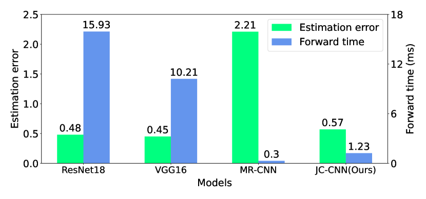
Figure 4. Comparison of CNN models for estimation error and network forward time.

4.2. Amplitude Ratio Estimation

Our algorithm for estimating the amplitude ratio is described in Algorithm 2. It should be noted that as described in Section 4.1, Algorithm 2 is only triggered when a collision is detected and the amplitude ratio needs to be estimated to perform the jamming cancellation. Our approach is inspired by the observation that the power of a receiving antenna during a collision comprises two independent, separable components for the legitimate signal $S$ and the jamming signal $J$. Suppose during time period $T$, the receiver collects $N$ digital RF samples from the analog input of antenna $i$, the received power $E^{T}_{i}$ can be written as:

(11) $$E^{T}_{i}=\frac{1}{N}\sum_{t=1}^{N}|h_{S_{i}}^{t}S^{t}+h_{J_{i}}^{t}J^{t}|^{2}$$

Given that the channel is slow-fading and not dependent on the instant time $t$, and because the sender’s signal $S$ and the jammer’s signal $J$ are uncorrelated, i.e. $\sum_{t=1}^{N}h^{t}_{S_{i}}S^{t}(h^{t}_{J_{i}}J^{t})^{*}=0$ and $\sum_{t=1}^{N}(h^{t}_{S_{i}}S^{t})^{*}h^{t}_{J_{i}}J^{t}=0$, Equation 11 becomes:

(12) $$E^{T}_{i}=\frac{1}{N}(|h_{S_{i}}|^{2}\sum_{t=1}^{N}|S^{t}|^{2})+\frac{1}{N}(|h_{J_{i}}|^{2}\sum_{t=1}^{N}|J^{t}|^{2})=E_{S_{i}}+E_{J_{i}}$$

To estimate $A_{J}=\frac{\left|h_{J_{1}}\right|}{\left|h_{J_{2}}\right|}=\sqrt{\frac{E_{J_{1}}}{E_{J_{2}}}}$ (where $E_{J_{i}}=\frac{1}{N}(|h_{J_{i}}|^{2}\sum_{t=1}^{N}|J^{t}|^{2})$), we need to measure $E_{S_{i}}=\frac{1}{N}(\left|h_{S_{i}}\right|^{2}\sum_{t=1}^{N}|S^{t}|^{2})$ for two antennas $i\in\{1,2\}$. To do this, we first determine whether the legitimate sender or the jammer transmits first, right before the collision (using the detection capability described in Section 4.1), then calculate the power accordingly. Here, we assume the sender’s power is stable during the transmission of a packet (slow fading channel), so the measurement of $E_{S_{i}}$ at the beginning of the collision can be used until the end of that collision. Our algorithm looks at period $T-1$ right before the collision, and identifies the transmitter in that period with parameter $I^{last}_{J}$ (which is updated in Algorithm 1 and utilized in Algorithm 2). If the sender appears in period $T-1$ (where $I^{last}_{J}=0$), we can measure $E_{S_{i}}$ and calculate $A_{J}$. Otherwise, we know that the jammer appears in period $T-1$, and we can measure $E_{J_{i}}$ and update $E_{S_{i}}$ with the current power $E_{i}$. It should be noted that in the latter case, the new $E_{S_{i}}$ is used until the end of the collision and should not be updated again if we detect a collision in the previous period.

Data: $E_{J_{i}},E_{S_{i}},1^{T-1}_{S_{i}}$ with $i\in\{1,2\}$, $I^{last}_{J}$, RF samples at $T$

Result: $A_{J}$

Measure the current power $E^{T}_{i}$ with $i\in\{1,2\}$;

if $I^{last}_{J}=1\textnormal{{\hskip 3.00003ptand \hskip 3.00003pt}}1^{T-1}_{S_{1}}\bigoplus 1^{T-1}_{S_{2}}=1$ then

       $E_{S_{1}}\leftarrow E^{T}_{1}-E_{J_{1}}$;

       $E_{S_{2}}\leftarrow E^{T}_{2}-E_{J_{2}}$;

      

end if

$A_{J}\leftarrow\sqrt{\frac{E^{T}_{1}-E_{S_{1}}}{E^{T}_{2}-E_{S_{2}}}}$

Algorithm 2 Amplitude Ratio Estimation

4.3. Estimation Smoothing

Unlike the estimations $I^{T}_{S_{1}},I^{T}_{S_{2}}$ which are discretized to the values of $0$ and $1$ for the signal detections, the real-valued estimations $P^{T}_{S_{1}},P^{T}_{S_{2}}$ are used directly to solve the jamming cancellation equation. This makes the cancellation process susceptible to the neural network’s estimation variations and outliers (Bishop, 2006). We improve the robustness of the phase shift estimation and the subsequent jamming cancellation process by stabilizing the estimations with the exponential smoothing function:

(13) $$\Delta_{\phi_{J}}=\Delta^{T}_{\phi_{J}}\lambda+\Delta^{cur}_{\phi_{J}}(1-\lambda)$$

where $\lambda$ controls the smoothness of the output. We note that after performing the cancellation for the current period, $\Delta^{cur}_{\phi_{J}}$ is updated to the current value of $\Delta_{\phi_{J}}$. With this, the phase shift estimation $\Delta_{\phi_{J}}$ is more stable which makes the jamming cancellation process more robust. We will show how the smoothing algorithm and $\lambda$ parameter impact the performance of the cancellation through experimental evaluations in Section 5.

5. Evaluation

In this section, we evaluate our CNN-based jamming cancellation approach in multiple settings of modulations and wireless channels. Using the techniques mentioned in Section 3.3, we collect RF samples transmitted by a sender and a jammer through coaxial cables to a receiver, and build a dataset containing $7,648,260$ real-valued data tensors of size $2\times 128\times 2$ reflecting $I/Q$ values of 128 RF samples collected by two antennas. Each data tensor is labeled by the phase shifts of signals embedded in the data (if the data is collected from the sender, or the jammer, or the combination of the two) and the signal indicators ($0$ for noise and $1$ for real signal) for their respective phases. The transmitters and receiver are implemented using GNURadio (gnu, 2021) running on ETTUS USRP B210 software-defined radios. The radios use differential BPSK, QPSK, 8-PSK and 16-QAM modulation schemes to transmit and receive at a center frequency of $795$ MHz. We split the dataset into three parts used for training, validation, and testing with the ratio $0.64:0.16:0.2$, respectively. Our trained CNN model is used for both over-the-cables evaluation (Section 5.2) and over-the-air evaluation (Section 5.3). We emphasize that while the CNN model is trained only using the data collected through cables, our jamming cancellation approach still performs well in over-the-air indoor environment with the presence of multi-path and other channel effects not experienced in the cabled environments.

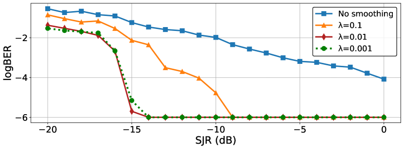
(a) Bit Error Rate.

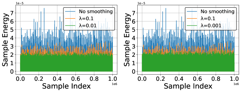
(b) Energy variation.

Figure 5. Estimation smoothing reduces energy fluctuation from cancellation and improves Bit Error Rate. Decreasing $\bm{\lambda}$ from $\bm{0.01}$ to $\bm{0.001}$ does not further improve the energy variation (Plot (b): $\bm{\lambda=0.01}$ (left) has similar variation to $\bm{\lambda=0.001}$ (right)). Similarly, for the Bit Error Rate (Plot (a)).

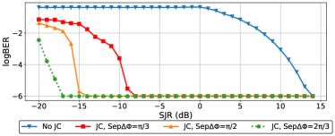
(a) BPSK

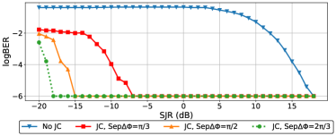
(b) QPSK

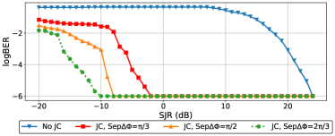
(c) 8-PSK

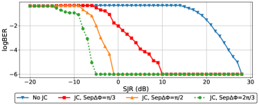
(d) 16-QAM

Figure 6. Bit Error Rate evaluation for over-the-cables experiments.

5.1. Neural Network Comparison

Beyond evaluating the performance of our novel approach, we are also interested in understanding the performance of the specific CNN architecture we proposed. Towards this goal, we compare it with existing CNN models from the literature, in terms of estimation error and network forward time (i.e., the elapsed time from when the network receives data to when it outputs estimations). In our setup, we train our CNN model (called JC-CNN), VGG16 (Simonyan and Zisserman, 2014), ResNet (He et al., 2016), and the modulation recognition CNN (MR-CNN) (O’Shea et al., 2016) and evaluate using the training and test set of our jamming detection and cancellation dataset, respectively. The models are implemented, trained, and tested using the Pytorch library (Paszke et al., 2019) and CUDA (NVIDIA et al., 2020) Version 10.2 running on a NVIDIA GeForce GTX 1080 GPU. We use Adam Optimizer (Kingma and Ba, 2017) and ReduceLROnPlateau learning rate scheduler (Zaheer et al., 2018) with initial learning rate $lr=0.005$ for the training of all models. The metric for estimation error is the combination loss denoted by Equation 9. To benchmark the forward time, we use Pytorch’s torch.cuda.synchronize wrapping around neural network’s forward propagation function to synchronize CUDA operations for accurate timing measurement. The final test loss and forward time are achieved by averaging over $20,000$ iterated measurements, and illustrated in Figure 4. It is clear that our JC-CNN model outperforms MR-CNN in the correctness of the estimations, with the test error of $0.57$ compared to $2.21$ of MR-CNN (over $3.8$ times lower), while is slightly less accurate than VGG-16 and ResNet18 with the test losses of $0.45$ and $0.48$, respectively. However, our model is $12.95$ times faster than ResNet18 and $8.3$ times faster than VGG16. Therefore, the JC-CNN model has a better optimization of speed and accuracy for this task and is more suitable to deploy for real-time and embedded applications.

5.2. Over-The-Cables Evaluation

First, we evaluate the efficiency of the jamming cancellation approach in a relatively idealistic environment where RF signals propagate through coaxial cables, thus multi-path and other fading effects are absent. Our setup comprises a sender, a receiver and a jammer, where the sender and the jammer transmit modulated signals using differential BPSK, QPSK, 8-PSK and 16-QAM. The efficiency of jamming cancellation is measured by the Bit Error Rate metric, which we calculate by comparing and counting the error bits between the sent and the received signals (signals are recorded at the nodes and transferred to the host computer for calculation).

In Section 2.2 we show that the phase shift separation $Sep_{\Delta_{\phi}}=\left|\Delta_{\phi_{S}}-\Delta_{\phi_{J}}\right|$ being very small can cause negative effects to the legitimate signal even when the jamming signal is completely removed. In our experiment, the transmitters are connected to the sender by identical coaxial cables, in which $Sep_{\Delta_{\phi}}\approx 0$. To address this, we introduce an artificial channel effect by shifting the phases of the antennas. Depending on the shifting, $Sep_{\Delta_{\phi}}$ will receive a different value. We discuss the impact of $Sep_{\Delta_{\phi}}$ on the efficiency of the jamming cancellation in the evaluation below.

Impact of Phase Separation. Figure 8 shows the Bit Error Rate (BER) evaluation considering four cases: No jamming cancellation ($JC$) is applied, and jamming cancellation is applied with three values of $Sep_{\Delta_{\phi}}:\frac{\pi}{3},\frac{\pi}{2},$ and $\frac{2\pi}{3}$. In this evaluation, the jamming cancellation algorithm uses the estimation smoothing with parameter $\lambda=0.01$. First, it is clear to see that our cancellation approach can achieve very high jamming resistance: It allows the receiver to operate at BER of $10^{-6}$ with the Signal-to-Jamming Ratio of $-18$dB (i.e., the jammer is 63 times more powerful than the legitimate signal) for QPSK with $Sep_{\Delta_{\phi}}=\frac{2\pi}{3}$. Interestingly, when compared with the case of no cancellation, our approach achieves over $30$dB gain for all modulations when operating at a BER of under $10^{-4}$ (e.g. $31$ dB for BPSK and $34$ dB for QPSK with $Sep_{\Delta_{\phi}}=\frac{2\pi}{3}$). In addition, we also see that the jamming cancellation performs better as $Sep_{\Delta_{\phi}}$ gets bigger. For instance, the jamming resistance when operating at a BER of $10^{-6}$ with BPSK modulation drops by $3$dB when $Sep_{\Delta_{\phi}}$ decreases from $\frac{2\pi}{3}$ to $\frac{\pi}{2}$, and by $9$dB when it decreases to $\frac{\pi}{3}$. It is easy to see the same trend for the other modulations. This limitation is intrinsic to multi-antenna jamming cancelation as the receiver cannot resolve two transmitter that are aligned with it. Furthermore, we also see that the efficiency of our jamming cancellation when using 8-PSK and 16-QAM is lower compared to BPSK and QPSK, which is expected because they have smaller distance between the constellation points and thus are more prone to bit errors (Proakis and Salehi, 2008).

Impact of Estimation Smoothing. We investigate the impact of phase shift estimation smoothing on the jamming cancellation with the Bit Error Rate evaluation shown in Figure 5(a). In this case, we use BPSK signals and $Sep_{\Delta_{\phi}}=\frac{\pi}{2}$. It is clear to see that the smoothing significantly improves the jamming resistance: We achieve $11$ and $15$ dB gain with $\lambda=0.1$ and $0.01$ when operating at BER below $10^{-4}$, respectively. This effect can also be seen in Figure 5(b), where the estimation smoothing helps stabilizing the energy of the samples and reduce both the degree and the frequency of energy variation, resulting in better BER. Finally, setting $\lambda$ to $0.01$ makes the energy more stable and yields better jamming resistance ($-14$ dB of SJR compared to $-9$dB for $\lambda=0.1$ when operating at BER=$10^{-6}$, while decreasing $\lambda$ to $0.001$ does not improve the performance further. Therefore, we selected $\lambda=0.01$ for all later evaluations.

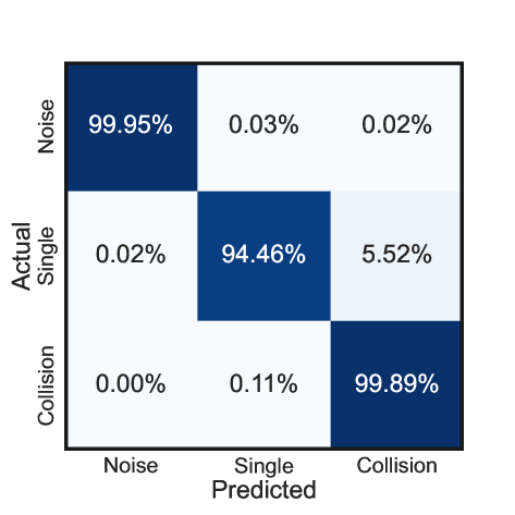
Figure 7. Confusion matrix of channel state classification.

5.3. Over-The-Air Evaluation

Jammer Detection. We conduct over-the-air experiments to assess the ability of our CNN model to detect a jammer detection, in an environment different from the one used for training, i.e., model trained on data recorded through cables is evaluated for over-the-air without re-training. Similar to over-the-cables experiments, our setup consists of a sender, a receiver, and a jammer. We use differential BPSK, QPSK, 8-PSK and 16-QAM modulations for the transmissions. The testbed is positioned in an indoor environment, where there are common RF-blocking and reflecting objects such as a PC, monitor, walls, and desks. To evaluate the detection capability, we focus on the classification of three channel states: (1) When there is no transmission and the channel is clear, (2) when there is a single transmission, and (3) when there are two transmissions (from the sender and the jammer) causing collisions. We note that in the second case, the transmitter being the sender or the jammer is decided by the decoding check in Algorithm 1. Table 1 and Figure 7 depict the classification results, in which the CNN classifies three states: Noise (no transmission), Single (one transmission) and Collision (two transmissions). Our CNN model achieves 97.44% accuracy, where it can reach over $99\%$ accuracy for the Noise and Collision states while the accuracy of Single state prediction is only about $5\%$ lower. We also get high scores for other metrics, over 0.98 for both Precision, Recall and F1-Score. The results justify the capability of our CNN model to identify the current channel state, and more importantly, the presence of a jammer (by recognizing collisions with $99.89\%$ accuracy) in the realistic environment without the needs to retrain the model trained in the idealistic environment (i.e. coaxial cables).

Accuracy	Precision	Recall	F1-Score
97.44%	0.9818	0.981	0.9809

Table 1. Channel classification results with different metrics.

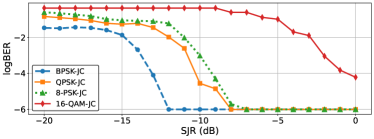
(a) $1^{st}$ configuration

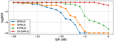
(b) $2^{nd}$ configuration

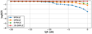
(c) $3^{rd}$ configuration

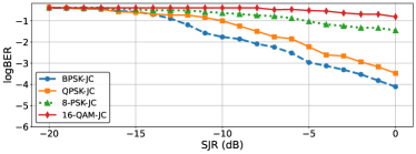
(d) $4^{th}$ configuration

Figure 8. Bit Error Rate evaluation for over-the-air experiments. When the legitimate signal and the jamming signal are phase-aligned (i.e. $\bm{Sep_{\Delta_{\phi}}\approx 0}$), removing the jamming signal from the received signal also heavily degrades the legitimate signal and impacts the Bit Error Rate.

Jamming Resistance. To demonstrate the jamming resistance capability of our approach in over-the-air environments, we devise four setup configurations for our experiments. In each configuration, we randomly position the jammer, while the locations of the sender and the receiver remain fixed. To evaluate, we measure the Bit Error Rate (BER) of the received data for every case. As discussed in the previous sections, different configurations will introduce different phase shift separations $Sep_{\Delta_{\phi}}$ that impact the quality of the signal resulting from the jamming cancellation. To measure $Sep_{\Delta_{\phi}}$ for each configuration, we use the cross-correlation technique presented in Section 3.3. The BER evaluation results in Figure 8 show that the receiver equipped with the jamming cancellation ($JC$) achieves the best jamming resistance for both BPSK, QPSK, 8-PSK and 16-QAM modulations with the $1^{st}$ configuration whose phase shift separation is biggest (measured in Table 2). More specifically, we can operate with BPSK at BER of $10^{-6}$ under a Signal-to-Jamming Ratio (SJR) of $-12$ dB in the $1^{st}$ configuration, and under a SJR of -6 dB in the $2^{nd}$ configuration (which has the second-largest $Sep_{\Delta_{\phi}}$), while we only achieve the BER of down to $10^{-3}$ and $10^{-4}$ under a SJR of $0$ dB for the $3^{rd}$ and $4^{th}$ configurations, respectively. In the $3^{rd}$ configuration when the sender’s signal and the jammer’s signal are nearly phase-aligned ($Sep_{\Delta_{\phi}}$ has the lowest value of $0.34$), the resulting signal is especially weak and causes a high BER, i.e., over $10^{-2}$ for all modulations at SJR = $0$ except BPSK. This impact of $Sep_{\Delta_{\phi}}$ justifies the theory in Section 2.2 and our findings in over-the-cables experiments. Furthermore, we can also see that the efficiency of the jamming cancellation decreases as the modulation order increases. More specifically, compared to the case of BPSK modulation, using QPSK drops the jamming resistance by $2-3$dB, while the drop is $4-5$dB for 8-PSK and over $10$dB for 16-QAM. This is expected because higher-order modulations have a smaller distance between the constellation points that cause higher probability of bit errors (Proakis and Salehi, 2008). However, we note that the BER when not using our Jamming Cancellation is $\approx 0.5$ (theoretical maximum) for all the transmission settings and configurations shown in Figure 8. Therefore, the results indicate the efficiency of our jamming cancellation approach, as well as the universality for anti-jamming multiple modulation and in different environments not present during the training of the CNN model.

Configuration	$1^{st}$	$2^{nd}$	$3^{rd}$	$4^{th}$
$Sep_{\Delta_{\phi}}$	2.22 rad	1.44 rad	0.34 rad	0.56 rad

Table 2. $Sep_{\Delta_{\phi}}$ measurements of over-the-air configurations.

6. Discussion and Related work

The results show that our approach can perform well under the impact of multi-path, albeit Equation 3 only shows a single channel gain for either the jammer or the sender in the received signal. Nonetheless, the results do not contradict the cancellation theory. As explained in (Vo-Huu et al., 2013), the sum of the channel gains of all the paths from the sender (or the jammer) to the receiver can be viewed as a new channel gain of the line-of-sight path between the receiver and the sender/jammer being put in a different location. Therefore, Equation 3 is also applicable in this case, and the jamming cancellation is still effective.

It is demonstrated that the performance of multi-antenna jamming cancellation systems degrades when the emitters are phase-aligned. The next challenge is how to ensure a desirable phase shift separation to distinguish between two emitters and cancel the unwanted signal. To address this, it is intuitive to use and optimize a larger antenna array to exploit the diversity of multi-antenna and enhance the robustness of cancellation. On that account, exploring optimized settings of antenna array for robust jamming cancellation would be an interesting direction for our future work.

Traditional anti-jamming at the physical layer has been relying on spread spectrum techniques, which require the coordinating nodes to pre-share a secret key. Recent research efforts have addressed that limitation for FHSS (Lazos et al., 2009; Strasser et al., 2008, 2009; Xiao et al., 2012), or DSSS (Pöpper et al., 2009; Liu et al., 2010), or both (Jin et al., 2009). Nonetheless, these approaches are designed with the specific goal to remove the pre-shared secret and not to counter powerful jammers, i.e., a few orders stronger than the sending node.

There has been efforts on multi-antenna anti-jamming designed specifically for MIMO system (Yan et al., 2014; Zeng et al., 2017). Compared to those approaches, our work is unique in the sense that we do not need training sequences or pilots for channel estimation. In a recent work (Vo-Huu et al., 2013), the authors develop a hybrid anti-jamming system that utilizes mechanical antenna steering and multi-antenna software cancellation. While this approach achieves high jamming resiliency, the efficiency of the cancellation relies heavily on the after-effect of mechanical steering to the received jamming signal, while our CNN-based cancellation can operate even when the interference remains powerful.

In addition, researchers have spent significant efforts mitigating jammers at higher layers such as MAC (Awerbuch et al., 2008; Richa et al., 2010), network layer (Dong et al., 2009), cross-layer (Chiang and Hu, 2010) or timing channel between datalink and network layers (Xu et al., 2008). Nonetheless, the need for an efficient, resilient anti-jamming technique for physical layer security is still very important because of the fact that high-power jammers are increasingly easy to build nowadays.

Advances in Machine Learning and Deep Learning have been utilized in various domains including anti-jamming. In (Han et al., 2017), Deep Reinforcement Learning is used to derive an optimal frequency hopping strategy to evade jammers. In (Erpek et al., 2019), the authors investigate Generative Adversarial Network for both jamming strategies and defense. Meanwhile, the anti-jamming capability of Convolutional Neural Networks - a vital Deep Learning building block, remains unexplored. Convolutional Neural Networks were successful in various tasks of wireless communications, such as modulation recognition (O’Shea et al., 2016), and RF emissions detection and classification (Nguyen et al., 2021). To the best of our knowledge, our anti-jamming approach is the first work in the literature that utilizes CNNs to detect and cancel jammers efficiently. We achieve over $99\%$ accuracy for detecting jammers and can enhance a RF receiver to achieve a Bit Error Rate as low as $10^{-6}$ while facing an adversary at 18dB higher power than the legitimate signal. Our approach is agnostic to the communication link, i.e., does not require modifications to the link modulation, thus can be used as an universal anti-jamming and interference-cancelling module for existing technologies and systems.

References

- (1)
- gnu (2021) 2021. GNURadio. https://www.gnuradio.org
- Abdel-Hamid et al. (2014) Ossama Abdel-Hamid, Abdel-rahman Mohamed, Hui Jiang, Li Deng, Gerald Penn, and Dong Yu. 2014. Convolutional Neural Networks for Speech Recognition. IEEE/ACM Transactions on Audio, Speech, and Language Processing 22, 10 (2014), 1533–1545. https://doi.org/10.1109/TASLP.2014.2339736
- Awerbuch et al. (2008) Baruch Awerbuch, Andrea Richa, and Christian Scheideler. 2008. A jamming-resistant MAC protocol for single-hop wireless networks. In Proceedings of the twenty-seventh ACM symposium on Principles of distributed computing. 45–54.
- Bishop (2006) Christopher M. Bishop. 2006. Pattern Recognition and Machine Learning (Information Science and Statistics). Springer-Verlag, Berlin, Heidelberg.
- Chiang and Hu (2010) Jerry T Chiang and Yih-Chun Hu. 2010. Cross-layer jamming detection and mitigation in wireless broadcast networks. IEEE/ACM Transactions on networking 19, 1 (2010), 286–298.
- Dong et al. (2009) Jing Dong, Reza Curtmola, and Cristina Nita-Rotaru. 2009. Practical defenses against pollution attacks in intra-flow network coding for wireless mesh networks. In Proceedings of the second ACM conference on Wireless network security. 111–122.
- Erpek et al. (2019) Tugba Erpek, Yalin E. Sagduyu, and Yi Shi. 2019. Deep Learning for Launching and Mitigating Wireless Jamming Attacks. IEEE Transactions on Cognitive Communications and Networking 5, 1 (March 2019), 2–14. https://doi.org/10.1109/TCCN.2018.2884910
- FCC (2020) FCC. 2020. Jammer Enforcement. https://www.fcc.gov/general/jammer-enforcement.
- FCC (2022) FCC. 2022. FCC Upholds Fine for Jammer Used to Block Workers’ Phone Use. https://www.fcc.gov/document/fcc-upholds-fine-jammer-used-block-workers-phone-use.
- Ge et al. ([n.d.]) Rong Ge, Sham M Kakade, Rahul Kidambi, and Praneeth Netrapalli. [n.d.]. The Step Decay Schedule: A Near Optimal, Geometrically Decaying Learning Rate Procedure For Least Squares. In Advances in Neural Information Processing Systems.
- Glorot et al. (2011) Xavier Glorot, Antoine Bordes, and Yoshua Bengio. 2011. Deep Sparse Rectifier Neural Networks. In Proceedings of the Fourteenth International Conference on Artificial Intelligence and Statistics (Proceedings of Machine Learning Research, Vol. 15). 315–323.
- Han et al. (2017) Guoan Han, Liang Xiao, and H. Vincent Poor. 2017. Two-dimensional anti-jamming communication based on deep reinforcement learning. In 2017 IEEE International Conference on Acoustics, Speech and Signal Processing (ICASSP). 2087–2091. https://doi.org/10.1109/ICASSP.2017.7952524
- He et al. (2016) Kaiming He, Xiangyu Zhang, Shaoqing Ren, and Jian Sun. 2016. Deep Residual Learning Image Recognition. In CVPR’16.
- Ioffe and Szegedy (2015) Sergey Ioffe and Christian Szegedy. 2015. Batch Normalization: Accelerating Deep Network Training by Reducing Internal Covariate Shift. In ICML.
- Jin et al. (2009) Tao Jin, Guevara Noubir, and Bishal Thapa. 2009. Zero Pre-Shared Secret Key Establishment in the Presence of Jammers. In Proceedings of the Tenth ACM International Symposium on Mobile Ad Hoc Networking and Computing (New Orleans, LA, USA) (MobiHoc ’09). Association for Computing Machinery, New York, NY, USA, 219–228. https://doi.org/10.1145/1530748.1530779
- Kalchbrenner et al. (2014) Nal Kalchbrenner, Edward Grefenstette, and Phil Blunsom. 2014. A Convolutional Neural Network for Modelling Sentences. arXiv:1404.2188 [cs.CL]
- Kingma and Ba (2017) Diederik P. Kingma and Jimmy Ba. 2017. Adam: A Method for Stochastic Optimization. arXiv:1412.6980 [cs.LG]
- Lazos et al. (2009) Loukas Lazos, Sisi Liu, and Marwan Krunz. 2009. Mitigating Control-Channel Jamming Attacks in Multi-Channel Ad Hoc Networks. In Proceedings of the Second ACM Conference on Wireless Network Security (Zurich, Switzerland) (WiSec ’09). Association for Computing Machinery, New York, NY, USA, 169–180. https://doi.org/10.1145/1514274.1514299
- Liu et al. (2010) Yao Liu, Peng Ning, Huaiyu Dai, and An Liu. 2010. Randomized Differential DSSS: Jamming-Resistant Wireless Broadcast Communication. In 2010 Proceedings IEEE INFOCOM. 1–9. https://doi.org/10.1109/INFCOM.2010.5462156
- Nguyen et al. (2021) Hai N Nguyen, Marinos Vomvas, Triet Vo-Huu, and Guevara Noubir. 2021. Wideband, Real-time Spectro-Temporal RF Identification. In Proceedings of the 19th ACM International Symposium on Mobility Management and Wireless Access. 77–86.
- NVIDIA et al. (2020) NVIDIA, Péter Vingelmann, and Frank H.P. Fitzek. 2020. CUDA, release: 10.2.89. https://developer.nvidia.com/cuda-toolkit
- O’Shea et al. (2016) Timothy J. O’Shea, Johnathan Corgan, and T. Charles Clancy. 2016. Convolutional Radio Modulation Recognition Networks. In Engineering Applications of Neural Networks.
- Paszke et al. (2019) Adam Paszke, Sam Gross, Francisco Massa, Adam Lerer, James Bradbury, Gregory Chanan, Trevor Killeen, Zeming Lin, Natalia Gimelshein, Luca Antiga, Alban Desmaison, Andreas Kopf, Edward Yang, Zachary DeVito, Marin Raison, Alykhan Tejani, Sasank Chilamkurthy, Benoit Steiner, Lu Fang, Junjie Bai, and Soumith Chintala. 2019. PyTorch: An Imperative Style, High-Performance Deep Learning Library. In Advances in Neural Information Processing Systems 32. 8024–8035.
- Pöpper et al. (2009) Christina Pöpper, Mario Strasser, and Srdjan Capkun. 2009. Jamming-resistant broadcast communication without shared keys.. In USENIX security Symposium. 231–248.
- Proakis and Salehi (2008) John G Proakis and Masoud Salehi. 2008. Digital communications.
- Project Zero (2017) Project Zero. 2017. Over The Air: Exploiting Broadcom’s Wi-Fi Stack. https://www.crowdsupply.com/fairwaves/xtrx
- Richa et al. (2010) Andrea Richa, Christian Scheideler, Stefan Schmid, and Jin Zhang. 2010. A jamming-resistant mac protocol for multi-hop wireless networks. In International Symposium on Distributed Computing. Springer, 179–193.
- Schulz et al. (2016) M. Schulz, D. Wegemer, and M. Hollick. 2016. DEMO: Using NexMon, the C-based WiFi firmware modification framework. In Proceedings of the 9th ACM Conference on Security and Privacy in Wireless and Mobile Networks (WiSec ’16). ACM.
- Simonyan and Zisserman (2014) K. Simonyan and A. Zisserman. 2014. Very deep convolutional networks for large-scale image recognition. In arXiv:1409.1556.
- Strasser et al. (2008) Mario Strasser, Christina Popper, Srdjan Capkun, and Mario Cagalj. 2008. Jamming-resistant Key Establishment using Uncoordinated Frequency Hopping. In 2008 IEEE Symposium on Security and Privacy (sp 2008). 64–78. https://doi.org/10.1109/SP.2008.9
- Strasser et al. (2009) Mario Strasser, Christina Pöpper, and Srdjan Čapkun. 2009. Efficient Uncoordinated FHSS Anti-Jamming Communication. In Proceedings of the Tenth ACM International Symposium on Mobile Ad Hoc Networking and Computing (New Orleans, LA, USA) (MobiHoc ’09). Association for Computing Machinery, New York, NY, USA, 207–218. https://doi.org/10.1145/1530748.1530778
- Vo-Huu et al. (2013) Triet D. Vo-Huu, Erik-Oliver Blass, and Guevara Noubir. 2013. Counter-Jamming Using Mixed Mechanical and Software Interference Cancellation. In Proceedings of the Sixth ACM Conference on Security and Privacy in Wireless and Mobile Networks (Budapest, Hungary) (WiSec ’13). Association for Computing Machinery, New York, NY, USA, 31–42. https://doi.org/10.1145/2462096.2462103
- Wilhelm et al. (2011) Matthias Wilhelm, Ivan Martinovic, Jens B. Schmitt, and Vincent Lenders. 2011. Short paper: reactive jamming in wireless networks: how realistic is the threat?. In Proceedings of the fourth ACM conference on Wireless network security (Hamburg, Germany) (WiSec ’11). ACM, New York, NY, USA, 47–52. https://doi.org/10.1145/1998412.1998422
- Xiao et al. (2012) Liang Xiao, Huaiyu Dai, and Peng Ning. 2012. Jamming-Resistant Collaborative Broadcast Using Uncoordinated Frequency Hopping. IEEE Transactions on Information Forensics and Security 7, 1 (2012), 297–309. https://doi.org/10.1109/TIFS.2011.2165948
- Xu et al. (2008) Wenyuan Xu, Wade Trappe, and Yanyong Zhang. 2008. Anti-jamming timing channels for wireless networks. In Proceedings of the first ACM conference on Wireless network security. 203–213.
- Yan et al. (2014) Qiben Yan, Huacheng Zeng, Tingting Jiang, Ming Li, Wenjing Lou, and Y. Thomas Hou. 2014. MIMO-based jamming resilient communication in wireless networks. In IEEE INFOCOM 2014 - IEEE Conference on Computer Communications. 2697–2706. https://doi.org/10.1109/INFOCOM.2014.6848218
- Zaghari et al. (2020) Bahareh Zaghari, Alex S. Weddell, Kamran Esmaeili, Imran Bashir, Terry J. Harvey, Neil M. White, Patrick Mirring, and Ling Wang. 2020. High-Temperature Self-Powered Sensing System for a Smart Bearing in an Aircraft Jet Engine. IEEE Transactions on Instrumentation and Measurement 69 (2020), 6165–6174.
- Zaheer et al. (2018) Manzil Zaheer, Sashank Reddi, Devendra Sachan, Satyen Kale, and Sanjiv Kumar. 2018. Adaptive Methods for Nonconvex Optimization. In Advances in Neural Information Processing Systems, S. Bengio, H. Wallach, H. Larochelle, K. Grauman, N. Cesa-Bianchi, and R. Garnett (Eds.), Vol. 31. Curran Associates, Inc. https://proceedings.neurips.cc/paper/2018/file/90365351ccc7437a1309dc64e4db32a3-Paper.pdf
- Zeng et al. (2017) Huacheng Zeng, Chen Cao, Hongxiang Li, and Qiben Yan. 2017. Enabling jamming-resistant communications in wireless MIMO networks. In 2017 IEEE Conference on Communications and Network Security (CNS). IEEE, 1–9.