Generative Principal Component Analysis
Abstract
In this paper, we study the problem of principal component analysis with generative modeling assumptions, adopting a general model for the observed matrix that encompasses notable special cases, including spiked matrix recovery and phase retrieval. The key assumption is that the underlying signal lies near the range of an -Lipschitz continuous generative model with bounded -dimensional inputs. We propose a quadratic estimator, and show that it enjoys a statistical rate of order , where is the number of samples. We also provide a near-matching algorithm-independent lower bound. Moreover, we provide a variant of the classic power method, which projects the calculated data onto the range of the generative model during each iteration. We show that under suitable conditions, this method converges exponentially fast to a point achieving the above-mentioned statistical rate. We perform experiments on various image datasets for spiked matrix and phase retrieval models, and illustrate performance gains of our method to the classic power method and the truncated power method devised for sparse principal component analysis.
I Introduction
Principal component analysis (PCA) is one of the most popular techniques for data processing and dimensionality reduction [1], with an abundance of applications such as image recognition [2], gene expression data analysis [3], and clustering [4, 5]. PCA seeks to find the directions that capture maximal variances in vector-valued data. In more detail, letting be realizations of a random vector with a population covariance matrix , PCA aims to reconstruct the top principal eigenvectors of . The first principal eigenvector can be computed as follows:
| (1) |
where the empirical covariance matrix is defined as , with . In addition, subsequent principal eigenvectors can be estimated by similar optimization problems subject to being orthogonal to the previous vectors.
PCA is consistent in the conventional setting where the dimension of the data is relatively small compared to the sample size [6], but leads to rather poor estimates in the high-dimensional setting where . In particular, it has been shown in various papers that the empirical principal eigenvectors are no longer consistent estimates of their population counterparts [7, 8, 9, 10]. In order to tackle the curse of dimensionality, a natural approach is to impose certain structural constraints on the principal eigenvectors. A common assumption is that the principal eigenvectors are sparse, and this gives rise to the problem of sparse principal component analysis (SPCA) [11]. In particular, for recovering the top principal eigenvector, the optimization problem of SPCA is given by
| (2) |
where denotes the number of non-zero entries of , and represents the sparsity level. In addition to reducing the effective number of parameters, the sparsity assumption also enhances the interpretability [11].
Departing momentarily from the PCA problem, recent years have seen tremendous advances in deep generative models in a wide variety of real-world applications [12]. This has motivated a new perspective of the related problem of compressed sensing (CS), in which the standard sparsity assumption is replaced by a generative modeling assumption. That is, the underlying signal is assumed to lie near the range of a (deep) generative model [13]. The authors of [13] characterized the number of samples required to attain an accurate reconstruction, and also presented numerical results on image datasets showing that compared to sparsity-based methods, generative priors can lead to large reductions (e.g., a factor of to ) in the number of measurements needed to recover the signal up to a given accuracy. Additional numerical and theoretical results concerning inverse problems using generative models have been provided in [14, 15, 16, 17, 18, 19, 20, 21, 22, 23, 24], among others.
In this paper, following the developments in both PCA/SPCA and inverse problems with generative priors, we study the use of generative priors in principal component analysis (GPCA), which gives a generative counterpart of SPCA in (2), formulated as follows:
| (3) |
where is a (pre-trained) generative model, which we assume has a range contained in the unit sphere of .111Similarly to [25, 26], we assume that the range of is contained in the unit sphere for convenience. Our results readily transfer to general (unnormalized) generative models by considering its normalized version. See Remark 1 for a detailed discussion. Similarly to SPCA, the motivation for this problem is to incorporate prior knowledge on the vector being recovered (or alternatively, a prior preference), and to permit meaningful recovery and theoretical bounds even in the high-dimensional regime .
I-A Related Work
In this subsection, we summarize some relevant works, which can roughly be divided into (i) the SPCA problem, and (ii) signal recovery with generative models.
SPCA: It has been proved that the solution of the SPCA problem in (2) attains the optimal statistical rate [27], where is the number of samples, is the ambient dimension, and is the sparsity level of the first principal eigenvector. However, due to the combinatorial constraint, the computation of (2) is intractable. To address this computational issue, in recent years, an extensive body of practical approaches for estimating sparse principal eigenvectors have been proposed in the literature, including [28, 29, 30, 31, 32, 33, 11, 34, 35, 36, 37, 38, 39, 40], just to name a few.
Notably, statistical guarantees for several approaches have been provided. The authors of [38] propose the truncated power method (TPower), which adds a truncation operation to the power method to ensure the desired level of sparsity. It is shown that this approach attains the optimal statistical rate under appropriate initialization. Most approaches for SPCA only focus on estimating the first principal eigenvector, with a certain deflation method [41] being leveraged to reconstruct the rest. However, there are some exceptions; for instance, an iterative thresholding approach is proposed in [42], and is shown to attain a near-optimal statistical rate when estimating multiple individual principal eigenvectors. In addition, the authors of [43] propose a regression-type method that gives an optimal principal subspace estimator. Both works [42, 43] rely on the assumption of a spiked covariance model to ensure a good initial vector. To avoid the spiked covariance model assumption, the work [44] proposes a two-stage procedure that attains the optimal subspace estimator in polynomial time.
Signal recovery with generative models: Since the seminal work [13], there has been a substantial volume of papers studying various inverse problems with generative priors. One of the problems more closely related to PCA is spectral initialization in phase retrieval, which amounts to solving an eigenvalue problem. Phase retrieval with generative priors has been studied in [45, 46, 47, 48, 49, 50, 51]. In particular, the work [45] models the underlying signal as being in the range of a fully-connected ReLU neural network with no offsets, and all the weight matrices of the ReLU neural network are assumed to have i.i.d. zero-mean Gaussian entries. In addition, the neural network needs to be sufficiently expansive in the sense that , where is the width of the -th layer. Under these assumptions, the authors establish favorable global optimization landscapes for the corresponding objective, and derive a near-optimal sample complexity upper bound. They minimize the objective function directly over the latent space in using gradient descent, which may suffer from local minima in general optimization landscapes [46, 52].
In [50], the assumptions on the neural network are similar to those in [45], relaxing to general activation functions (beyond ReLU) and . The authors focus on the high dimensional regime where with the ratio being fixed, and assume that the input vector in is drawn from a separable distribution. They derive sharp asymptotics for the information-theoretically optimal performance and for the associated approximate message passing (AMP) algorithm. Both works [45, 50] focus on noiseless phase retrieval. When only making the much milder assumption that the generative model is Lipschitz continuous, with no assumption on expansiveness, Gaussianity, and offsets, a spectral initialization step (similar to that of sparse phase retrieval) is typically required in order to accurately reconstruct the signal [53, 54]. The authors of [51] propose an optimization problem similar to (3) for the spectral initialization for phase retrieval with generative models. It was left open in [51] how to solve (or approximate sufficiently accurately) the optimization problem in practice.
Understanding the eigenvalues of spiked random matrix models has been a central problem of random matrix theory, and spiked matrices have been widely used in the statistical analysis of SPCA. Recently, theoretical guarantees concerning spiked matrix models with generative priors have been provided in [55, 56]. In particular, in [55], the assumptions are similar to those in [50], except that the neural network is assumed to have exactly one hidden layer. The Bayes-optimal performance is analyzed, and it is shown that the AMP algorithm can attain this optimal performance. In addition, the authors of [55] propose the linearized approximate message passing (LAMP) algorithm, which is a spectral algorithm specifically designed for single-layer feedforward neural networks with no bias terms. The authors show its superiority to classical PCA via numerical results on the Fashion-MNIST dataset. In [56], the same assumptions are made as those in [45] on the neural network, and the authors demonstrate the benign global geometry for a nonlinear least squares objective. Similarly to [45], the objective is minimized over using a gradient descent algorithm, which can get stuck in local minima for general global geometries.
I-B Contributions
The main contributions of this paper are threefold:
-
•
We study eigenvalue problems with generative priors (including GPCA), and characterize the statistical rate of a quadratic estimator similar to (3) under suitable assumptions. We also provide a near-matching algorithm-independent lower bound.
-
•
We propose a variant of the classic power method, which uses an additional projection operation to ensure that the output of each iteration lies in the range of a generative model. We refer to our method as projected power method (PPower). We further show that under appropriate conditions (most notably, assuming exact projections are possible), PPower obtains a solution achieving the statistical rate that is attained by the quadratic estimator.
-
•
For spiked matrix and phase retrieval models, we perform numerical experiments on image datasets, and demonstrate that when the number of samples is relatively small compared to the ambient dimension, PPower leads to significantly better performance compared to the classic power method and TPower.
Compared to the above-mentioned works that use generative models, we make no assumption on expansiveness, Gaussianity, and offsets for the generative model, and we consider a data model that simultaneously encompasses both spiked matrix and phase retrieval models, among others.
I-C Notation
We use upper and lower case boldface letters to denote matrices and vectors respectively. We write for a positive integer , and we use to denote the identity matrix in . A generative model is a function , with latent dimension , ambient dimension , and input domain . We focus on the setting where . For a set and a generative model , we write . We use to denote the spectral norm of a matrix . We define the -ball for . represents the unit sphere in . The symbols are absolute constants whose values may differ from line to line.
II Problem Setup
In this section, we formally introduce the problem, and overview some important assumptions that we adopt. Except where stated otherwise, we will focus on the following setting:
-
•
We have a matrix satisfying
(4) where is a perturbation matrix, and is assumed to be positive semidefinite (PSD). For PCA and its constrained variants, and can be thought of as the empirical and population covariance matrices, respectively.
-
•
We have an -Lipschitz continuous generative model . For convenience, similarly to that in [25], we assume that .
Remark 1.
For a general (unnormalized) -Lipschitz continuous generative model , we can instead consider a corresponding normalized generative model as in [51], where for some , and . Then, the Lipschitz constant of becomes . For a -layer neural network, we typically have [13]. Thus, we can set to be as small as without changing the scaling laws, which makes the dependence on very mild.
-
•
We aim to solve the following eigenvalue problem with a generative prior:222To find the top rather than top one principal eigenvectors that are in the range of a generative model, we may follow the common approach to use the iterative deflation method for PCA/SPCA: Subsequent principal eigenvectors are derived by recursively removing the contribution of the principal eigenvectors that are calculated already under the generative model constraint. See for example [41].
(5) Note that since , we do not need to impose the constraint . Since is not restricted to being an empirical covariance matrix, (5) is more general than GPCA in (3). However, we slightly abuse terminology and also refer to (5) as GPCA.
-
•
To approximately solve (5), we use a projected power method (PPower), which is described by the following iterative procedure:333In similar iterative procedures, some works have proposed to replace by for some to improve convergence, e.g., see [57].
(6) where is the projection function onto ,444That is, for any , . We will implicitly assume that the projection step can be performed accurately, e.g., [57, 52, 58], though in practice approximate methods might be needed, e.g., via gradient descent [52] or GAN-based projection methods [59]. and the initialization vector may be chosen either manually or randomly, e.g., uniform over . Often the initialization vector plays an important role and we may need a careful design for it. For example, for phase retrieval with generative models, as mentioned in [51, Section V], we may choose the column corresponding to the largest diagonal entry of as the starting point. See also [38, Section 3] for a discussion on the initialization strategy for TPower devised for SPCA. We present the algorithm corresponding to (6) in Algorithm 1.
Remark 2.
To tackle generalized eigenvalue problems encountered in some specific applications, there are variants of the projected power method, which combine a certain power iteration with additional operations to ensure sparsity or enforce other constraints. These applications include but not limited to sparse PCA [35, 38], phase synchronization [60, 61], the hidden clique problem [62], the joint alignment problem [63], and cone-constrained PCA [57, 64]. For example, under the simple spiked Wigner model [65] for the observed data matrix with the underlying signal being assumed to lie in a convex cone, the authors of [57] show that cone-constrained PCA can be computed efficiently via a generalized projected power method. In general, the range of a Lipschitz-continuous generative model is non-convex and not a cone. In addition, we consider a matrix model that is more general than the spiked Wigner model.
Algorithm 1 A projected power method for GPCA (PPower) Input: , number of iterations , pre-trained generative model , initial vector
Procedure: Iterate for , and return
Although it is not needed for our main results, we first state a lemma (proved in Appendix A) that establishes a monotonicity property with minimal assumptions, only requiring that is PSD; see also Proposition 3 of [38] for an analog in sparse PCA. By comparison, our main results in Section IV will make more assumptions, but will also provide stronger guarantees. Note that the PSD assumption holds, for example, when , or when is a sample covariance matrix.
Lemma 1.
For any , let . Then, if is PSD, the sequence for in (6) is monotonically non-decreasing.
III Specialized Data Models and Examples
In this section, we make more specific assumptions on , starting with the following.
Assumption 1 (Assumption on ).
Assume that is PSD with eigenvalues . We use (a unit vector) to represent the eigenvector of that corresponds to .
In the following, it is useful to think of is being close to the range of the generative model . In the special case of (3), letting be the number of samples, it is natural to derive that the upper bound of grows linearly in for some positive constant such as or (with high probability; see, e.g., [66, Corollary 5.35]). In the following, we consider general scenarios with depending on samples (see below for specific examples). Similarly to [38], we may consider a restricted version of , leading to the following.
Assumption 2 (Assumption on ).
Let be two (arbitrary) finite sets in satisfying . Then, we have for all and that
| (7) |
where is an absolute constant. In addition, we have .555For the spectral norm of , one often expects an even tighter bound , but we use to simplify the analysis of our examples. Moreover, at least under the typical scaling where is polynomial in [13], the upper bound for can be easily relaxed to for any positive constant , without affecting the scaling of our derived statistical rate.
The following examples show that when the number of measurements is sufficiently large, the data matrices corresponding to certain spiked matrix and phase retrieval models satisfy the above assumptions with high probability. Short proofs are given in Appendix B for completeness.
Example 1 (Spiked covariance model).
In the spiked covariance model [8, 67], the observed vectors are of the form
| (8) |
where are orthonormal vectors that we want to estimate, while and are independent and identically distributed. In addition, are positive constants that dictate the signal-to-noise ratio (SNR). To simplify the exposition, we focus on the rank-one case and drop the subscript . Let
| (9) |
and .666To avoid non-essential complications, is typically assumed to be known [8]. Then, satisfies Assumption 1 with , , and . In addition, letting , the Bernstein-type inequality [66, Proposition 5.10] for the sum of sub-exponential random variables yields that for any finite sets , when , with probability , satisfies (7) in Assumption 2. Moreover, standard concentration arguments give with probability .
Remark 3.
We can also consider the simpler spiked Wigner model [65, 68] where , with the signal being a unit vector, being an SNR parameter, and being a symmetric matrix with entries drawn i.i.d. (up to symmetry) from . In this case, when is sufficiently large, with high probability, and similarly satisfy Assumptions 1 and 2 respectively.
Example 2 (Phase retrieval).
Let be a matrix having i.i.d. entries, and let be the -th row of . For some unit vector , suppose that the observed vector is , where the absolute value is applied element-wise.777Without loss of generality, we assume that is a unit vector. For a general signal , we may instead focus on estimating , and simply use to approximate . We construct the weighted empirical covariance matrix as follows [69, 51]:
| (10) |
where are positive constants, and for , . Let , where . Then, satisfies Assumption 1 with , , and . In addition, letting , we have similarly to Example 1 that satisfies Assumption 2 with high probability.
IV Main Results
Theorem 1.
We have stated this result as an upper bound on , which intuitively measures the distance between the 1D subspaces spanned by and . Note, however, that for any two unit vectors with , the distances and are equivalent up to constant factors, whereas if , then a similar statement holds for . See Appendix C for the precise statements.
In Theorem 1, the final term quantifies the effect of representation error. When there is no such error (i.e., ), under the scaling , , and , Theorem 1 simplifies to . This provides a natural counterpart to the statistical rate of order for SPCA mentioned in Section I-A. In Appendix J, we provide an algorithm-independent lower bound showing that this scaling cannot be improved in general.
Before providing our main theorem for PPower described in (6), we present the following important lemma, whose proof is presented in Appendix E. To simplify the statement of the lemma, we fix to be , though a more general form analogous to Theorem 1 is also possible.
Lemma 2.
Remark 4.
The assumption will be particularly satisfied when the range of only contains nonnegative vectors. As mentioned in various works studying nonnegative SPCA [70, 71, 72], for several practical fields such as economics, bioinformatics, and computer vision, it is natural to assume that the underlying signal has no negative entries. More generally, the assumption can be removed if we additionally have that is also contained in the range of . For this case, when , we can instead derive an upper bound for .
Theorem 2.
Suppose that the assumptions on the data model are the same as those in Lemma 2, and assume that there exists such that with , where , and are both positive and scale as . Let , and in addition, suppose that with being large enough. Then, we have after iterations of PPower (beyond ) that
| (13) |
i.e., this equation holds for all . Moreover, if then , whereas if , we have exponentially fast convergence via the following contraction property: There exists a constant such that for , it holds that
| (14) |
Regarding the assumption , we note that when , this condition can be viewed as having a good initialization. For both Examples 1 and 2, we have . Thus, for the spiked covariance and phase retrieval models corresponding to these examples, the assumption reduces to for a sufficiently small positive constant , which results in a mild assumption. Such an assumption is also required for the projected power method devised for cone-constrained PCA under the simple spiked Wigner model, with the underlying signal being assumed to lie in a convex cone; see [57, Theorem 3]. Despite using a similar assumption on the initialization, our proof techniques are significantly different from [57]; see Appendix G for discussion.
When is polynomial in , Theorem 2 reveals that we have established conditions under which PPower in (6) converges exponentially fast to a point achieving the statistical rate of order . From the algorithm-independent lower bound established in Appendix J, we know that this statistical rate nearly matches the optimal rate for GPCA. We highlight that Theorem 2 partially addresses the computational-to-statistical gap (e.g., see [73, 45, 55, 56]) for spiked matrix recovery and phase retrieval under a generative prior, though closing it completely would require efficiently finding a good initialization and addressing the assumption of exact projections.
Perhaps the main caveat to Theorem 2 is that it assumes the projection step can be performed exactly. However, this is a standard assumption in analyses of projected gradient methods, e.g., see [52], and both gradient-based projection and GAN-based projection have been shown to be highly effective in practice [52, 59].
V Experiments
In this section, we experimentally study the performance of Algorithm 1 (PPower). We note that these experiments are intended as a simple proof of concept rather than seeking to be comprehensive, as our contributions are primarily theoretical. We compare with the truncated power method (TPower) devised for SPCA proposed in [38, Algorithm 1] and the vanilla power method (Power) that performs the iterative procedure . For a fair comparison, for PPower, TPower, and Power, we use the same initial vector. Specifically, as mentioned in [51, Section V], we choose the initialization vector as the column of that corresponds to its largest diagonal entry. For all three algorithms, the total number of iterations is set to be . To compare the performance across algorithms, we use the scale-invariant Cosine Similarity metric (in absolute value) defined as , where is the ground-truth signal to estimate, and denotes the output vector of the algorithm. Note that we take the absolute value because any estimate or its negative are considered equally good in all the baseline methods we compare with.
The experiments are performed on the MNIST [74], Fashion-MNIST [75] and CelebA [76] datasets, with the numerical results for the Fashion-MNIST and CelebA datasets being presented in Appendices H and I. The MNIST dataset consists of images of handwritten digits. The size of each image is , and thus . To reduce the impact of local minima, we perform random restarts, and choose the best among these. The cosine similarity is averaged over the test images, and also over these random restarts. The generative model is set to be a pre-trained variational autoencoder (VAE) model with latent dimension . We use the VAE model trained by the authors of [13] directly, for which the encoder and decoder are both fully connected neural networks with two hidden layers, with the architecture being . The VAE is trained by the Adam optimizer with a mini-batch size of and a learning rate of . The projection step is solved by the Adam optimizer with a learning rate of and steps. In each iteration of TPower, the calculated entries are truncated to zero except for the largest entries, where is a tuning parameter. Since for TPower, is usually selected as an integer larger than the true sparsity level, and since it is unlikely that the image of the MNIST dataset can be well approximated by a -sparse vector with , we choose a relatively large , namely . Similarly to [13] and other related works, we only report the results on a test set that is unseen by the pre-trained VAE model, i.e., the training of and the PPower computations do not use common data.888All experiments are run using Python 3.6 and Tensorflow 1.5.0, with a NVIDIA GeForce GTX 1080 Ti 11GB GPU. The corresponding code is available at https://github.com/liuzq09/GenerativePCA.
-
1.
Spiked covariance model (Example 1): The numerical results are shown in Figures 1 and 2. We observe from Figure 1 that Power and TPower attain poor reconstructions, and the generative prior based method PPower attains significantly better reconstructions. To illustrate the effect of the sample size , we fix the SNR parameter and vary in . In addition, to illustrate the effect of the SNR parameter , we fix , and vary in . From Figure 2, we observe that for these settings of and , PPower always leads to a much higher cosine similarity compared to Power and TPower, which is natural given the more precise modeling assumptions used.
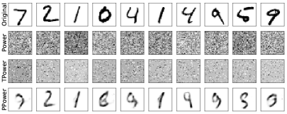
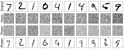
(a) and (b) and Figure 1: Examples of reconstructed images of the MNIST dataset for the spiked covariance model. 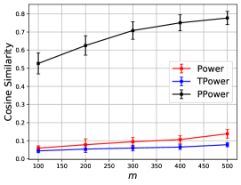
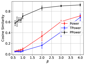
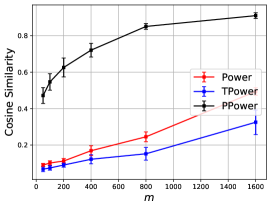
(a) Fixing and varying (b) Fixing and varying (c) Analog of (a) for phase ret. Figure 2: Quantitative comparisons of the performance of Power, TPower and PPower according to the Cosine Similarity for the MNIST dataset, under both the spiked covariance model (Left/Middle) and phase retrieval model (Right). -
2.
Phase retrieval (Example 2): The results are shown in Figure 2 (Right) and Figure 3. Again, we can observe that PPower significantly outperforms Power and TPower. In particular, for sparse phase retrieval, when performing experiments on image datasets, even for the noiseless setting, solving an eigenvalue problem similar to (5) can typically only serve as a spectral initialization step, with a subsequent iterative algorithm being required to refine the initial guess. In view of this, it is notable that for phase retrieval with generative priors, PPower can return meaningful reconstructed images for , which is small compared to .
VI Conclusion
We have proposed a quadratic estimator for eigenvalue problems with generative models, and we showed that this estimator attains a statistical rate of order . We also showed that this statistical rate is almost tight by providing a near-matching algorithm-independent lower bound. Furthermore, we provided a projected power method to efficiently solve (modulo the complexity of the projection step) the corresponding optimization problem, and showed that our method converges exponentially fast to a point achieving a statistical rate of order under suitable conditions.
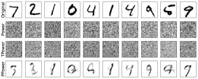 |

|
| (a) | (b) |
Appendix A Proof of Lemma 1 (Non-Decreasing Property of )
Appendix B Proofs for Spiked Matrix and Phase Retrieval Examples
Before proceeding, we present the following standard definitions.
Definition 1.
A random variable is said to be sub-Gaussian if there exists a positive constant such that for all . The sub-Gaussian norm of a sub-Gaussian random variable is defined as .
Definition 2.
A random variable is said to be sub-exponential if there exists a positive constant such that for all . The sub-exponential norm of is defined as .
The following lemma states that the product of two sub-Gaussian random variables is sub-exponential, regardless of the dependence between them.
Lemma 3.
[77, Lemma 2.7.7] Let and be sub-Gaussian random variables (not necessarily independent). Then is sub-exponential, and satisfies
| (21) |
The following lemma provides a useful concentration inequality for the sum of independent sub-exponential random variables.
Lemma 4.
[66, Proposition 5.16] Let be independent zero-mean sub-exponential random variables, and . Then for every and , it holds that
| (22) |
where is an absolute constant. In particular, with , we have
| (23) |
The widely-used notion of an -net is introduced as follows.
Definition 3.
Let be a metric space, and fix . A subset is said be an -net of if, for all , there exists some such that . The minimal cardinality of an -net of , if finite, is denoted and is called the covering number of (at scale ).
The following lemma provides a useful upper bound for the covering number of the unit sphere.
Lemma 5.
[66, Lemma 5.2] The unit Euclidean sphere equipped with the Euclidean metric satisfies for every that
| (24) |
The following lemma provides an upper bound for the spectral norm of a symmetric matrix.
Lemma 6.
[66, Lemma 5.4] Let be a symmetric matrix, and let be an -net of for some . Then,
| (25) |
With the above auxiliary results in place, we provide the proofs of Assumption 2 holding for the two examples described in Section III.
B-A Spiked Covariance Model (Example 1)
As per Assumption 2, fix two finite signal sets and . For , we have and a direct calculation gives . Recall also that , , and . It follows that for any , we have that is sub-Gaussian, with the sub-Gaussian norm being upper bounded by . Similarly, we have for any that . Applying Lemma 3, we deduce that is sub-exponential, with the sub-exponential norm being upper bounded by . In addition, from (9) and , we have
| (26) | ||||
| (27) |
and we observe that . Then, from Lemma 4, we obtain that for any satisfying , the following holds with probability (recall that may vary from line to line):
| (28) |
where we note that the assumption ensures that the first term is dominant in the minimum in (23). Taking a union bound over all and , and setting , we obtain with probability that (7) holds (with being a fixed positive constant).
Next, we bound for fixed , but this time consider (different from the above ) satisfying . In this case, we can follow the above analysis (with and both replaced by ), but the assumption means that when applying Lemma 4, the second term in the minimum in (23) is now the dominant one. As a result, for any satisfying , and any , we have with probability that
| (29) | ||||
| (30) |
From Lemma 5, there exists an -net of satisfying . Taking a union bound over all , and setting , we obtain with probability that
| (31) |
Then, from Lemma 6, we have
| (32) |
B-B Phase Retrieval (Example 2)
Let and . It is shown in [51, Lemma 8] that
| (33) |
which implies
| (34) |
Then, for any and , we have
| (35) | ||||
| (36) |
Since each has i.i.d. entries, we observe that is sub-exponential with the sub-exponential norm being upper bounded by . In addition, from (33), we have . Then, from Lemma 4, we obtain that for any satisfying , with probability ,
| (37) |
Taking a union bound over all and , and setting , we obtain that with probability , (7) holds as desired (with being a fixed positive constant). In addition, similarly to (32), we have with probability that .
Appendix C Equivalence of Distances
The following lemma gives a useful equivalence between two distances.
Lemma 7.
For any pair of unit vectors with , we have
| (38) |
Moreover, if , then the same holds with replaced by .
Appendix D Proof of Theorem 1 (Guarantee on the Global Optimum)
Let the singular value decomposition (SVD) of be
| (47) |
where , and is an orthonormal matrix with the first column being . For , let the -th column of be . Then, we have
| (48) | ||||
| (49) | ||||
| (50) |
where we use in (50).
In addition, for any and any , we have
| (51) | ||||
| (52) |
In particular, when is symmetric, we obtain
| (53) |
Let be a -net of ; from [66, Lemma 5.2], we know that there exists such a net with
| (54) |
Since is -Lipschitz continuous, we have that is a -net of . We write
| (55) |
where satisfies . Suppose that ; if this is not the case, we can use analogous steps to obtain an upper bound for instead of . We have
| (56) | |||
| (57) | |||
| (58) | |||
| (59) | |||
| (60) | |||
| (61) | |||
| (62) | |||
| (63) | |||
| (64) | |||
| (65) | |||
| (66) | |||
| (67) | |||
| (68) | |||
| (69) | |||
| (70) | |||
| (71) |
where:
- •
-
•
(60) follows since are an eigenvalue-eigenvector pair for with ;
- •
- •
-
•
(63) follows from and ;
-
•
(64) follows since ;
- •
- •
- •
- •
- •
-
•
(70) follows from the triangle inequality;
-
•
(71) follows by substituting , along with the assumptions , , and .
From (71), we have the following when :
| (72) |
As mentioned earlier, if , we have the same upper bound as in (72) for . Therefore, we obtain
| (73) | ||||
| (74) | ||||
| (75) | ||||
| (76) |
where (73) follows from (40), (75) follows from , and (76) follows from (72).
Appendix E Proof of Lemma 2 (Auxiliary Result for PPower Analysis)
By the assumption , for any and , we have
| (77) |
which is seen by noting that when comparing with (in accordance with projection mapping to the closest point), as long as , the comparison reduces to comparing with , so is invariant to positive scaling of .
Let and . Then, we have . Since , we have
| (78) |
This is equivalent to
| (79) |
and expanding the square gives
| (80) |
Note also that from , we obtain , which we will use throughout the proof.
For , let be a -net of ; from Lemma 5, there exists such a net with
| (81) |
By the -Lipschitz continuity of , we have that is a -net of . We write
| (82) |
where satisfies , and satisfies . Then, we have
| (83) |
which follows from and . In the following, we control the two terms in (83) separately.
-
1.
The term : We decompose and , where and . Since , we have . In addition, we have and . Recall that in (47), we write the SVD of as . Since , we can write as . In addition, since , we have . Hence, by the Cauchy-Schwarz inequality, we have
(84) (85) (86) (87) (88) Therefore, we obtain
(89) (90) (91) (92) - 2.
Note that . Hence, and using (80), (83), (92), and (96), we obtain
| (97) |
Using , , and similarly , we obtain from (97) that
| (98) |
Since and , this is equivalent to
| (99) |
This equation is of the form (where and ), and using a simple application of the quadratic formula,999Since the leading coefficient of the quadratic is positive, must lie in between the two associated roots. This yields , from which the inequality gives (100). we obtain
| (100) | ||||
| (101) |
where we use the assumption and set in (101).
Appendix F Proof of Theorem 2 (Main Theorem for PPower)
Suppose for the time being that (13) holds for at least one index (we will later verify that this is the case), and let be the smallest such index. Thus, we have
| (102) |
Note that according to the theorem statement, is bounded away from zero. Using and the assumption that with being large enough, we deduce from (102) that is sufficiently small such that
| (103) |
Next, using the assumption , we write
| (104) |
Then, from Lemma 2, we obtain
| (105) | ||||
| (106) | ||||
| (107) |
where (106) follows from (102)–(103), and (107) follows from (104). Thus, we have transferred (102) from to , and proceeding by induction, we obtain
| (108) |
for al .
Next, we consider . Again using Lemma 2 (with ), we have
| (109) |
where we recall that , and note that the denominator in the second term of (109) follows since . Supposing that (otherwise, the above analysis for alone is sufficient), we have that (13) is reversed at :
| (110) |
This means that we can upper bound the second term in (109) by , which gives
| (111) |
Squaring both sides, expanding, and canceling the norms (which all equal one), we obtain
| (112) |
and by induction, we obtain that is monotonically increasing.
Recall that we assume that , and that is the smallest integer such that (13) holds. To verify that is finite and upper bound , we consider the following three cases:
-
•
(or equivalently, ): In this case, (109) gives (or , which we already addressed above). Thus, we have , as stated in the theorem.
-
•
(or equivalently, and ): Since is monotonically increasing, for any positive integer with , by applying Lemma 2 (or (109)) multiple times, we obtain101010In simpler notation, if , then we get , then , and so on, and then we can apply for .
(113) (114) Then, if we choose such that
(115) we obtain from (114) that
(116) (117) (118) (119) where (117) follows from , (118) follows from (115) and , and (119) follows from , which implies . Observe that (119) coincides with (13), and since , we obtain from (115) that as desired.
-
•
(or equivalently, and ): Recall that we only need to focus on the case . This means that (110) holds, implying that we can upper bound the second term in (109) by , yielding
(120) (121) (122) where . With the distance to shrinking by a constant factor in each iteration according to (122), and the initial distance being at most due to the vectors having unit norm, we deduce that iterations suffice to ensure that (13) holds for .
Appendix G Comparison of Analysis to [57]
As mentioned in Section IV, our analysis is significantly different from that of [57] despite using a similar assumption on the initialization. We highlight the differences as follows:
-
1.
Perhaps the most significant difference is that the proof of [57, Theorem 3] is highly dependent on the Moreau decomposition, which is only valid for a closed convex cone (see [57, Definition 1.2]). In particular, the Moreau decomposition needs to be used at the beginning of the proof of [57, Theorem 3], such as Eqs. (18) and (19) in the supplementary material therein. We do not see a way for the proof to proceed without the Moreau decomposition, and our may be very different from a convex cone.
- 2.
-
3.
In the PPower method in [57], the authors need to add with to the observed data matrix to improve the convergence. In particular, they mention in the paragraph before the statement of Theorem 3 that “the memory term is necessary for our proof technique to go through”. In contrast, our proof of Theorem 2 does not require adding such terms, even when our data model is restricted to the spiked Wigner model considered in [57].
-
4.
We consider a matrix model that is significantly more general than the spiked Wigner model studied in [57].
Appendix H Numerical Results for the Fashion-MNIST Dataset
The Fashion-MNIST dataset consists of Zalando’s article images with a training set of examples and a test set of examples. The size of each image in the Fashion-MNIST dataset is also , and thus .
The generative model is set to be a variational autoencoder (VAE). The VAE architecture is summarized as follows.111111Further details of the architecture can be found at https://github.com/hwalsuklee/tensorflow-generative-model-collections. The generator has latent dimension and four layers. The first two are fully connected layers with the architecture , and with ReLU activation functions. The output of the second layer, reshaped to , is forwarded to a deconvolution layer with kernel size and stride . The third layer uses ReLU activations and has output size , where is the number of channels. The fourth layer is a deconvolution layer with kernel size and strides , and it uses ReLU activations and has output size , where the number of channels is .
The VAE is trained with a mini-batch size of , a learning rate of , and epochs. The remaining parameters are the same as those for the MNIST dataset.
For most images in the Fashion-MNIST dataset, the corresponding vectors are not sparse in the natural basis. Hence, to make a fairer comparison to the sparsity-based method TPower, we convert the original images to the wavelet basis, and perform TPower on these converted images. The obtained results of TPower are then converted back to the vectors in the natural basis. The corresponding method is denoted by TPowerW, with “W” referring to the conversion to images in the wavelet basis.
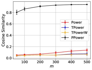
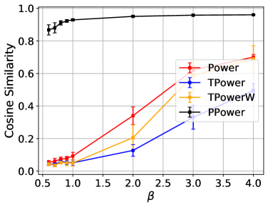
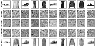
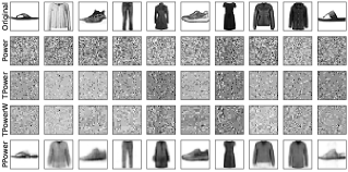
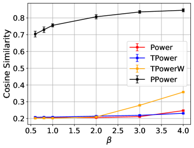
We perform two sets of experiments, considering the spiked covariance and phase retrieval models separately. The corresponding results are reported in Figures 4, 5, 6, and 7. From these figures, again, we can observe clear superiority of PPower compared to the baselines. As mentioned above,most of the images are not sparse in the natural basis, but we observe that (i) even for the sparsest images in Figures 4 and 6 (namely, those containing sandals), PPower significantly outperforms TPower, and (ii) generally, moving from TPower to TPowerW appears to provide at most marginal benefit.
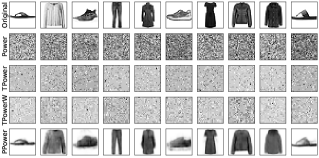 |
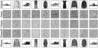
|
| (a) and | (b) and |
 |
|
| (a) Fixing and varying | (b) Fixing and varying |
 |
|
| (a) | (b) |
Appendix I Numerical Results for the CelebA Dataset
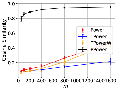
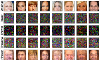
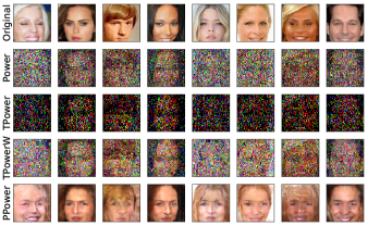
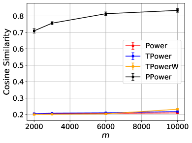
The CelebA dataset consists of more than face images of celebrities, where each input image is cropped to a RGB image with . The generative model is set to be a pre-trained Deep Convolutional Generative Adversarial Networks (DCGAN) model with latent dimension . We use the DCGAN model trained by the authors of [13] directly. We select the best estimate among random restarts. The Adam optimizer with steps and a learning rate of is used for the projection operator.
In each iteration of TPower and TPowerW, the calculated entries are truncated to zero except for the largest entries. For CelebA, is set to be . The remaining parameters are the same as those for the MNIST dataset. Here we focus on the spiked covariance model. The results are reported in Figures 8 and 9. From these figures, we can again observe the superiority of PPower compare to the baselines. While TPowerW does improve over TPower, its performance is still very limited.
 |
|
| (a) and | (b) and |
 |
|
| (a) Fixing and varying | (b) Fixing and varying |
Appendix J Lower Bound for the Reconstruction Error
In the following, we provide an algorithm-independent lower bound that serves as a counterpart to the upper bound given in Theorem 1. Note that here we consider the case that there is no representation error, which amounts to having in Theorem 1.
Theorem 3.
Given positive values of and such that is sufficiently large, and positive integer parameters and , there exists an -Lipschitz continuous generative model (for suitably-chosen ), and a family of distributions on , such that any estimator (depending on ) must satisfy
| (123) |
where expectation is taken over randomness of (whose distribution depends on ); moreover, the distributions satisfy the following properties:
-
•
There are independent samples drawn independently from with for some constants , and is the corresponding non-centered sample covariance matrix:
(124) - •
Before proving the theorem, we present some useful lemmas.
J-A Auxiliary Results for Theorem 3
We first state a standard lemma from [78] based on Fano’s inequality (see also [79]), using generic notation.
Lemma 8.
[78, Lemma 3] Let be an integer and index a collection of probability measures on a measurable space . Let be a pseudometric121212A pseudometric is a generalization of a metric in which the distance between two distinct points can be zero. on and suppose that for all ,
| (125) |
and
| (126) |
where denotes the Kullback-Leibler (KL) divergence between two probability measures and . Then, every -measurable estimator satisfies
| (127) |
where is the average with respect to .
In addition, we have the following lemma concerning the KL divergence between -fold products of Gaussian probability measures.
Lemma 9.
J-B Proof of Theorem 3
To prove the lower bound, we follow the construction technique from [25, Appendix C], who proved the existence of a generative model (with being a suitably-chosen integer multiple of ) such that
| (130) |
where and are positive constants, is the -th entry of , and denotes the set of -group-sparse vectors in , i.e., the coefficients are arranged into disjoint groups of size , and exactly one coefficient in each group is non-zero. In addition, we have that is -Lipschitz continuous with the Lipschitz constant being [25]
| (131) |
For any , let
| (132) |
Then, from (130)–(131), when , we obtain
| (133) |
and
| (134) |
Then, adapting an idea from [25], we claim that for any , there exists a subset such that:
-
•
for some universal constant ;
-
•
for all distinct pairs , it holds that .
For completeness, a proof of this claim is given at Appendix J-C. From Lemma 7, we obtain for all distinct pairs that
| (135) |
Fix , and for each , let
| (136) |
Since , it immediately follows that the eigenvalues of are , in accordance with Assumption 1.
Since Theorem 3 concerns the worst-case , it suffices to prove hardness within an arbitrary restricted set. Accordingly, we consider for all possible choices of . As stated in the theorem, when , the samples are drawn from the -fold product of (i.e., ), which we denote by , and is given by (124). The fact that Assumption 2 holds for any such is shown in a similar manner to Example 1; the details are given in Appendix J-D for completeness.
From Lemma 9 and (135), we have for all distinct pairs that
| (137) |
where . By the assumption that and are fixed positive constants with , we also have that is a fixed positive constant. Then, from Lemma 8 and (135), we obtain
| (138) |
where is the average with respect to (leaving the dependence on implicit).
Recalling that , we now observe that by choosing to be on the order , we can ensure that
| (139) |
Combining this with the fact that and in particular for sufficiently large , it follows from (138) that
| (140) |
Substituting the chosen scaling of and the behavior of the Lipschitz constant in (133), this yields
| (141) |
for some positive constant .
The lower bound in (141) holds even for an algorithm that has access to the samples , whereas Theorem 3 concerns only having access to . Since is deterministic given (see (124)), the latter problem can only be more difficult. Hence, by identifying with in (141) and further upper bounding the maximum over by the maximum over all of , the proof of Theorem 3 is complete.
J-C Proof of the Claim Following (134)
Consider the set of length- binary-valued signals
| (142) |
where we recall that is an integer multiple of . For any fixed , we have
| (143) |
where the upper bound follows from that can be distinct with in at most blocks among the blocks, and there are at most choices in each block. We aim to construct a set such that for all distinct ,
| (144) |
Suppose that we construct by picking elements in uniformly at random. When adding the -th point to , the probability that this point violates (144) with respect to the previously added points is upper bounded by
| (145) |
Therefore, taking a union bound, we can bound the total probability that fails to satisfy (144), denoted , by
| (146) |
Then, under the condition
| (147) |
it holds that . This implies that we can choose a set such that both (144) and (147) are satisfied; moreover, in the latter, we can ensure that equality holds up to insignificant rounding.
For any (noting that the upper limit is the value such that ), setting
| (148) |
we find that , where is defined in (132). In addition, since we are considering binary-valued signals satisfying (144), we have for any that
| (149) |
Combined with the fact that we ensured (147) holds with equality (up to rounding), this completes the proof of the claim.
J-D Proof that Assumption 2 Holds for
Fix , and suppose that the samples are generated following the Gaussian distribution with . Let be the non-centered sample covariance matrix. Clearly, we have , and thus has mean zero.
We write , where . As per Assumption 2, fix two finite signal sets and . For any and , letting and , we have
| (150) | ||||
| (151) | ||||
| (152) |
We upper bound (152) using a concentration argument. We observe that . In addition, we have that for , is sub-Gaussian, and the sub-Gasusian norm is for some constant . Applying Lemma 3, we deduce that is sub-exponential, with the sub-exponential norm being upper bounded by . From Lemma 4, it follows that for any satisfying , the following holds with probability (recall that may vary from line to line):
| (153) |
where we note that the assumption ensures that the first term is dominant in the minimum in (23), and the last inequality uses . Taking a union bound over all and in (153), and setting , we obtain with probability that (7) holds.
Finally, similarly to Example 1, we also have with probability that
| (154) |
References
- [1] I. T. Jolliffe, Principal component analysis. Springer-Verlag, 1986.
- [2] P. J. Hancock, A. M. Burton, and V. Bruce, “Face processing: Human perception and principal components analysis,” Mem. Cogn., vol. 24, no. 1, pp. 26–40, 1996.
- [3] O. Alter, P. O. Brown, and D. Botstein, “Singular value decomposition for genome-wide expression data processing and modeling,” PNAS, vol. 97, no. 18, pp. 10 101–10 106, 2000.
- [4] C. Ding and X. He, “-means clustering via principal component analysis,” in Int. Conf. Mach. Learn. (ICML), 2004, p. 29.
- [5] Z. Liu and V. Tan, “The informativeness of -means for learning mixture models,” IEEE Trans. Inf. Theory, vol. 65, no. 11, pp. 7460–7479, 2019.
- [6] T. W. Anderson, “An introduction to multivariate statistical analysis,” Wiley New York, Tech. Rep., 1962.
- [7] B. Nadler, “Finite sample approximation results for principal component analysis: A matrix perturbation approach,” Ann. Stat., vol. 36, no. 6, pp. 2791–2817, 2008.
- [8] I. M. Johnstone and A. Y. Lu, “On consistency and sparsity for principal components analysis in high dimensions,” J. Am. Stat. Assoc., vol. 104, no. 486, pp. 682–693, 2009.
- [9] S. Jung and J. S. Marron, “PCA consistency in high dimension, low sample size context,” Ann. Stat., vol. 37, no. 6B, pp. 4104–4130, 2009.
- [10] A. Birnbaum, I. M. Johnstone, B. Nadler, and D. Paul, “Minimax bounds for sparse PCA with noisy high-dimensional data,” Ann. Stat., vol. 41, no. 3, p. 1055, 2013.
- [11] H. Zou, T. Hastie, and R. Tibshirani, “Sparse principal component analysis,” J. Comput. Graph. Stat., vol. 15, no. 2, pp. 265–286, 2006.
- [12] D. Foster, Generative Deep Learning : Teaching Machines to Paint, Write, Compose and Play. O’Reilly Media, Inc, USA, 2019.
- [13] A. Bora, A. Jalal, E. Price, and A. G. Dimakis, “Compressed sensing using generative models,” in Int. Conf. Mach. Learn. (ICML), 2017, pp. 537–546.
- [14] D. Van Veen, A. Jalal, M. Soltanolkotabi et al., “Compressed sensing with deep image prior and learned regularization,” https://arxiv.org/1806.06438, 2018.
- [15] M. Dhar, A. Grover, and S. Ermon, “Modeling sparse deviations for compressed sensing using generative models,” in Int. Conf. Mach. Learn. (ICML). PMLR, 2018, pp. 1214–1223.
- [16] R. Heckel and P. Hand, “Deep decoder: Concise image representations from untrained non-convolutional networks,” in Int. Conf. Learn. Repr. (ICLR), 2019.
- [17] Z. Liu and J. Scarlett, “Information-theoretic lower bounds for compressive sensing with generative models,” IEEE J. Sel. Areas Inf. Theory, vol. 1, no. 1, pp. 292–303, 2020.
- [18] A. Kamath, S. Karmalkar, and E. Price, “On the power of compressed sensing with generative models,” in Int. Conf. Mach. Learn. (ICML), 2020, pp. 5101–5109.
- [19] A. Jalal, L. Liu, A. G. Dimakis, and C. Caramanis, “Robust compressed sensing using generative models,” Conf. Neur. Inf. Proc. Sys. (NeurIPS), 2020.
- [20] Z. Liu and J. Scarlett, “The generalized Lasso with nonlinear observations and generative priors,” in Conf. Neur. Inf. Proc. Sys. (NeurIPS), vol. 33, 2020.
- [21] G. Ongie, A. Jalal, C. A. Metzler et al., “Deep learning techniques for inverse problems in imaging,” IEEE J. Sel. Areas Inf. Theory, vol. 1, no. 1, pp. 39–56, 2020.
- [22] J. Whang, Q. Lei, and A. G. Dimakis, “Compressed sensing with invertible generative models and dependent noise,” https://arxiv.org/2003.08089, 2020.
- [23] A. Jalal, S. Karmalkar, A. Dimakis, and E. Price, “Instance-optimal compressed sensing via posterior sampling,” in Int. Conf. Mach. Learn. (ICML), 2021.
- [24] T. V. Nguyen, G. Jagatap, and C. Hegde, “Provable compressed sensing with generative priors via Langevin dynamics,” https://arxiv.org/2102.12643, 2021.
- [25] Z. Liu, S. Gomes, A. Tiwari, and J. Scarlett, “Sample complexity bounds for -bit compressive sensing and binary stable embeddings with generative priors,” in Int. Conf. Mach. Learn. (ICML), 2020.
- [26] Z. Liu, S. Ghosh, J. Han, and J. Scarlett, “Robust -bit compressive sensing with partial Gaussian circulant matrices and generative priors,” https://arxiv.org/2108.03570, 2021.
- [27] V. Vu and J. Lei, “Minimax rates of estimation for sparse PCA in high dimensions,” in Int. Conf. Artif. Intell. Stat. (AISTATS). PMLR, 2012, pp. 1278–1286.
- [28] A. d’Aspremont, L. El Ghaoui, M. I. Jordan, and G. R. Lanckriet, “A direct formulation for sparse PCA using semidefinite programming,” SIAM Rev., vol. 49, no. 3, pp. 434–448, 2007.
- [29] V. Q. Vu, J. Cho, J. Lei, and K. Rohe, “Fantope projection and selection: A near-optimal convex relaxation of sparse PCA,” Conf. Neur. Inf. Proc. Sys. (NeurIPS), vol. 26, 2013.
- [30] X. Chang, F. Nie, Y. Yang et al., “Convex sparse PCA for unsupervised feature learning,” ACM T. Knowl. Discov. D., vol. 11, no. 1, pp. 1–16, 2016.
- [31] B. Moghaddam, Y. Weiss, and S. Avidan, “Spectral bounds for sparse PCA: Exact and greedy algorithms,” Conf. Neur. Inf. Proc. Sys. (NeurIPS), vol. 18, p. 915, 2006.
- [32] A. d’Aspremont, F. Bach, and L. El Ghaoui, “Optimal solutions for sparse principal component analysis.” J. Mach. Learn. Res., vol. 9, no. 7, 2008.
- [33] I. T. Jolliffe, N. T. Trendafilov, and M. Uddin, “A modified principal component technique based on the Lasso,” J. Comput. Graph. Stat., vol. 12, no. 3, pp. 531–547, 2003.
- [34] H. Shen and J. Z. Huang, “Sparse principal component analysis via regularized low rank matrix approximation,” J. Multivar. Anal., vol. 99, no. 6, pp. 1015–1034, 2008.
- [35] M. Journée, Y. Nesterov, P. Richtárik, and R. Sepulchre, “Generalized power method for sparse principal component analysis.” J. Mach. Learn. Res., vol. 11, no. 2, 2010.
- [36] M. Hein and T. Bühler, “An inverse power method for nonlinear eigenproblems with applications in -spectral clustering and sparse PCA,” in Conf. Neur. Inf. Proc. Sys. (NeurIPS), 2010, pp. 847–855.
- [37] V. Kuleshov, “Fast algorithms for sparse principal component analysis based on Rayleigh quotient iteration,” in Int. Conf. Mach. Learn. (ICML). PMLR, 2013, pp. 1418–1425.
- [38] X.-T. Yuan and T. Zhang, “Truncated power method for sparse eigenvalue problems,” J. Mach. Learn. Res., vol. 14, no. 4, 2013.
- [39] M. Asteris, D. S. Papailiopoulos, and G. N. Karystinos, “Sparse principal component of a rank-deficient matrix,” in Int. Symp. Inf. Theory (ISIT). IEEE, 2011, pp. 673–677.
- [40] D. Papailiopoulos, A. Dimakis, and S. Korokythakis, “Sparse PCA through low-rank approximations,” in Int. Conf. Mach. Learn. (ICML). PMLR, 2013, pp. 747–755.
- [41] L. W. Mackey, “Deflation methods for sparse PCA,” in Conf. Neur. Inf. Proc. Sys. (NeurIPS), vol. 21, 2008, pp. 1017–1024.
- [42] Z. Ma, “Sparse principal component analysis and iterative thresholding,” Ann. Stat., vol. 41, no. 2, pp. 772–801, 2013.
- [43] T. T. Cai, Z. Ma, and Y. Wu, “Sparse PCA: Optimal rates and adaptive estimation,” Ann. Stat., vol. 41, no. 6, pp. 3074–3110, 2013.
- [44] Z. Wang, H. Lu, and H. Liu, “Tighten after relax: Minimax-optimal sparse PCA in polynomial time,” Conf. Neur. Inf. Proc. Sys. (NeurIPS), vol. 2014, p. 3383, 2014.
- [45] P. Hand, O. Leong, and V. Voroninski, “Phase retrieval under a generative prior,” in Conf. Neur. Inf. Proc. Sys. (NeurIPS), 2018, pp. 9154–9164.
- [46] R. Hyder, V. Shah, C. Hegde, and M. S. Asif, “Alternating phase projected gradient descent with generative priors for solving compressive phase retrieval,” in Int. Conf. Acoust. Sp. Sig. Proc. (ICASSP). IEEE, 2019, pp. 7705–7709.
- [47] G. Jagatap and C. Hegde, “Algorithmic guarantees for inverse imaging with untrained network priors,” in Conf. Neur. Inf. Proc. Sys. (NeurIPS), vol. 32, 2019.
- [48] X. Wei, Z. Yang, and Z. Wang, “On the statistical rate of nonlinear recovery in generative models with heavy-tailed data,” in Int. Conf. Mach. Learn. (ICML), 2019, pp. 6697–6706.
- [49] F. Shamshad and A. Ahmed, “Compressed sensing-based robust phase retrieval via deep generative priors,” IEEE Sens. J., vol. 21, no. 2, pp. 2286–2298, 2020.
- [50] B. Aubin, B. Loureiro, A. Baker et al., “Exact asymptotics for phase retrieval and compressed sensing with random generative priors,” in Math. Sci. Mach. Learn. (MSML). PMLR, 2020, pp. 55–73.
- [51] Z. Liu, S. Ghosh, and J. Scarlett, “Towards sample-optimal compressive phase retrieval with sparse and generative priors,” https://arxiv.org/2106.15358, 2021.
- [52] V. Shah and C. Hegde, “Solving linear inverse problems using GAN priors: An algorithm with provable guarantees,” in Int. Conf. Acoust. Sp. Sig. Proc. (ICASSP). IEEE, 2018, pp. 4609–4613.
- [53] P. Netrapalli, P. Jain, and S. Sanghavi, “Phase retrieval using alternating minimization,” IEEE Trans. Sig. Proc., vol. 63, no. 18, pp. 4814–4826, 2015.
- [54] E. J. Candès, X. Li, and M. Soltanolkotabi, “Phase retrieval via Wirtinger flow: Theory and algorithms,” IEEE Trans. Inf. Theory, vol. 61, no. 4, pp. 1985–2007, 2015.
- [55] B. Aubin, B. Loureiro, A. Maillard et al., “The spiked matrix model with generative priors,” Conf. Neur. Inf. Proc. Sys. (NeurIPS), vol. 32, pp. 8366–8377, 2019.
- [56] J. Cocola, P. Hand, and V. Voroninski, “Nonasymptotic guarantees for spiked matrix recovery with generative priors,” in Conf. Neur. Inf. Proc. Sys. (NeurIPS), vol. 33, 2020.
- [57] Y. Deshpande, A. Montanari, and E. Richard, “Cone-constrained principal component analysis,” in Conf. Neur. Inf. Proc. Sys. (NeurIPS), 2014, pp. 2717–2725.
- [58] P. Peng, S. Jalali, and X. Yuan, “Solving inverse problems via auto-encoders,” IEEE J. Sel. Areas Inf. Theory, vol. 1, no. 1, pp. 312–323, 2020.
- [59] A. Raj, Y. Li, and Y. Bresler, “GAN-based projector for faster recovery with convergence guarantees in linear inverse problems,” in IEEE/CVF Int. Conf. Comp. Vision (ICCV), 2019.
- [60] N. Boumal, “Nonconvex phase synchronization,” SIAM J. Optim., vol. 26, no. 4, pp. 2355–2377, 2016.
- [61] H. Liu, M.-C. Yue, and A. Man-Cho So, “On the estimation performance and convergence rate of the generalized power method for phase synchronization,” SIAM J. Optim., vol. 27, no. 4, pp. 2426–2446, 2017.
- [62] Y. Deshpande and A. Montanari, “Finding hidden cliques of size in nearly linear time,” Found. Comput. Math., vol. 15, no. 4, pp. 1069–1128, 2015.
- [63] Y. Chen and E. J. Candès, “The projected power method: An efficient algorithm for joint alignment from pairwise differences,” Comm. Pure Appl. Math., vol. 71, no. 8, pp. 1648–1714, 2018.
- [64] Y. Yi and M. Neykov, “Non-sparse PCA in high dimensions via cone projected power iteration,” https://arxiv.org/2005.07587, 2020.
- [65] A. Perry, A. S. Wein, A. S. Bandeira, and A. Moitra, “Optimality and sub-optimality of PCA I: Spiked random matrix models,” Ann. Stat., vol. 46, no. 5, pp. 2416–2451, 2018.
- [66] R. Vershynin, “Introduction to the non-asymptotic analysis of random matrices,” https://arxiv.org/abs/1011.3027, 2010.
- [67] Y. Deshpande and A. Montanari, “Sparse PCA via covariance thresholding,” J. Mach. Learn. Res., vol. 17, no. 1, pp. 4913–4953, 2016.
- [68] H. W. Chung and J. O. Lee, “Weak detection of signal in the spiked Wigner model,” in Int. Conf. Mach. Learn. (ICML). PMLR, 2019, pp. 1233–1241.
- [69] H. Zhang, Y. Zhou, Y. Liang, and Y. Chi, “A nonconvex approach for phase retrieval: Reshaped Wirtinger flow and incremental algorithms,” J. Mach. Learn. Res., vol. 18, 2017.
- [70] R. Zass and A. Shashua, “Nonnegative sparse PCA,” in Conf. Neur. Inf. Proc. Sys. (NeurIPS). Citeseer, 2007, pp. 1561–1568.
- [71] C. D. Sigg and J. M. Buhmann, “Expectation-maximization for sparse and non-negative PCA,” in Int. Conf. Mach. Learn. (ICML), 2008, pp. 960–967.
- [72] M. Asteris, D. Papailiopoulos, and A. Dimakis, “Nonnegative sparse PCA with provable guarantees,” in Int. Conf. Mach. Learn. (ICML). PMLR, 2014, pp. 1728–1736.
- [73] T. Wang, Q. Berthet, and R. J. Samworth, “Statistical and computational trade-offs in estimation of sparse principal components,” Ann. Stat., vol. 44, no. 5, pp. 1896–1930, 2016.
- [74] Y. LeCun, L. Bottou, Y. Bengio, and P. Haffner, “Gradient-based learning applied to document recognition,” Proc. IEEE, vol. 86, no. 11, pp. 2278–2324, 1998.
- [75] H. Xiao, K. Rasul, and R. Vollgraf, “Fashion-MNIST: A novel image dataset for benchmarking machine learning algorithms,” https://arxiv.org/1708.07747, 2017.
- [76] Z. Liu, P. Luo, X. Wang, and X. Tang, “Deep learning face attributes in the wild,” in Int. Conf. Comput. Vis. (ICCV), 2015, pp. 3730–3738.
- [77] R. Vershynin, High-dimensional probability: An introduction with applications in data science. Cambridge university press, 2018, vol. 47.
- [78] B. Yu, “Assouad, Fano, and Le Cam,” in Festschrift for Lucien Le Cam. Springer, 1997, pp. 423–435.
- [79] A. B. Tsybakov, Introduction to nonparametric estimation. Springer, New York, 2009.