LeHDC: Learning-Based Hyperdimensional Computing Classifier

Abstract.

Thanks to the tiny storage and efficient execution, hyperdimensional Computing (HDC) is emerging as a lightweight learning framework on resource-constrained hardware. Nonetheless, the existing HDC training relies on various heuristic methods, significantly limiting their inference accuracy. In this paper, we propose a new HDC framework, called LeHDC, which leverages a principled learning approach to improve the model accuracy. Concretely, LeHDC maps the existing HDC framework into an equivalent Binary Neural Network architecture, and employs a corresponding training strategy to minimize the training loss. Experimental validation shows that LeHDC outperforms previous HDC training strategies and can improve on average the inference accuracy over 15% compared to the baseline HDC.

1. Introduction

Brain-inspired hyperdimensional computing (HDC) is raised to represent samples by projecting them to extremely high-dimensional vectors, i.e., hypervector (Kanerva, 2009). As an emerging method, HDC is a promising alternative to conventional machine learning models like deep neural networks (DNNs), with less storage usage and higher efficiency. Although HDC is not meant to replace DNNs on all complex classification tasks, it indeed shows impressive performance on lightweight tasks and fits well in highly resource-limited Internet-of-Things (IoTs) devices. Given these characteristics, the studies on HDC have been quickly proliferating, including energy efficiency improvement (Imani et al., 2019a, d) and applications on tiny devices (Imani et al., 2018; Thapa et al., 2021). Meanwhile, HDC models have also been adopted on various acceleration platforms, such as FPGA (Imani et al., 2019a), GPU (Kim et al., 2020), and in-memory computing (Karunaratne et al., 2020), thanks to their high parallelism capacity.

Depending on the format of hypervectors, HDC can be broadly divided into binary HDC and non-binary HDC: the hypervectors and computations in binary HDC are all binarized, while binarization is not used in non-binary HDC. Naturally, non-binary HDC contains richer information expression on hypervectors, but it also costs more computing resources than binary HDC. On the other hand, binary HDC consumes lower energy and resources and is more friendly to hardware implementation. More recently, some heuristic approaches, such as retraining (i.e., fine-tune the class hypervectors after initial training) (Imani et al., 2019a), have been proposed to improve the inference accuracy, making binary HDC achieve a competitive accuracy performance compared to its non-binary counterpart. Nonetheless, the initial training process for an HDC model, binary and non-binary, still heavily depends on a simple strategy of averaging the sample hypervectors to obtain class hypervectors. In other words, there have been no principled approaches to optimally train an HDC model and rigorously learn the class hypervectors that provide the best possible accuracy performance for HDC.

In this paper, we demonstrate for the first time that a binary HDC classifier is equivalent to a wide single-layer binary neural network (BNN). Specifically, the binary weights in the BNN can be viewed as the class hypervectors in binary HDC, and the Hamming distance between the encoded hypervector and the class hypervectors in binary HDC can be linearly transformed into multiplication of the encoded hypervector and the binary weights. By viewing the class hypervector training process from the BNN perspective, we reveal the key limitations of the current HDC training strategy: heavily relying on heuristic approaches to search for class hypervectors. To address this limitation, we propose a learning-based HDC training strategy, namely LeHDC. Specifically, LeHDC takes the sample hypervector as input, assigns one-hot labels, and optimizes the BNN weights in the training process. The binary weights in the BNN are trained with state-of-the-art learning algorithms, and consequently, these binary weights can be directly converted to class hypervectors for the binary HDC classification. The binary HDC with obtained class hypervectors can achieve significantly higher accuracy than the current retraining strategies. Importantly, LeHDC introduces a completely new training process, but does not modify the encoding or inference processes used in the existing HDC. As a result, LeHDC can be integrated into any existing HDC framework to improve the accuracy performance, yet without any extra resource or execution overhead during the inference.

The main contributions of this work are as follows:

• We transform the existing binary HDC classifier into an equivalent BNN, and then reveal the key limitations in the current HDC training process that limit them from obtaining the optimal class hypervectors and achieving the best accuracy.

• We propose a new training strategy, LeHDC, on binary HDC classification, by leveraging state-of-the-art BNN learning algorithms. To the best of our knowledge, this is the first work using learning-based methods to train HDC classifications in a principled manner.

• We show empirically that LeHDC can significantly outperform current HDC models and provide over $15\%$ accuracy improvement against the baseline HDC, while introducing zero resource and time overhead during inference.

Our paper organization is: In Sec. 2, we briefly discuss the HDC classification and current training strategies. Sec. 3 reveals the limitations of the current HDC training process and equivalently expresses the HDC model in a wide single-layer BNN structure. Sec. 4 illustrates the proposed training strategy in LeHDC, and Sec. 5 presents the feasibility of our strategy and compares the performance with other training strategies. The conclusion and discussion on our work are addressed in Sec. 6.

2. HDC Classification Tasks

Binary HDC has been emerging as a novel paradigm that represent attributes with hyperdimensional bi-polar vectors $\{1,-1\}^{D}$ (Kanerva, 2009). For a specific sample $\textbf{F}=\{f_{1},f_{2},...,f_{N}\}$ where $f_{i}$ is the value of the $i$-th feature for $i=1,\cdots,N$, its feature positions and feature values are represented by randomly generated hypervectors, whose dimension (e.g., $D=10,000$) is much larger than the number of features/values. In a typical HDC model (Imani et al., 2019a), feature position hypervectors ($\mathcal{F}$) are orthogonal to identify an individual feature, i.e., the normalized Hamming distance $Hamm(\mathcal{F}_{i},\mathcal{F}_{j})\approx 0.5,i,j\in\{1,2,...,N\}$. Differently, feature value hypervectors ($\mathcal{V}$) are correlated to reflect the correlations in real values, i.e., $Hamm(\mathcal{V}_{f_{i}},\mathcal{V}_{f_{j}})\propto\frac{|f_{i}-f_{j}|}{max-min}$, where $f_{i}$ and $f_{j}$ are two samples in the value range, $f_{i},f_{j}\in[min,max]$.

2.1. Binary HDC

Binary HDC costs much lower power and computational resources, and is also the mainstream HDC framework (Imani et al., 2019a). By binding feature position hypervectors and value hypervectors, a sample can be described as a new hypervector ($\mathcal{H}\in\{1,-1\}^{D}$):

(1) $$\mathcal{H}=sgn\left(\sum_{i=1}^{N}\mathcal{F}_{i}\circ\mathcal{V}_{f_{i}}\right)$$

where this sample has $N$ features, and $\circ$ denotes the Hadamard product to multiply two hypervectors in element-wise. $sgn(\cdot)$ is the sign function to binarize the sum of hypervectors; here we assume $sgn(0)$ is randomly assigned with 1 or -1. In general, an HDC classifier can use record-based or $N$-gram-based encoders (Ge and Parhi, 2020). While our training approach applies to any encoding methods (including advanced ones (Yu et al., 2022) based on sophisticated feature extractions), for a concrete case study, we adopt the commonly-used record-based encoding which, shown in Eq. 1, has higher accuracy than the $N$-gram-based method for many applications (Ge and Parhi, 2020). Note that LeHDC does not modify the encoding process, and hence can work with any encoders.

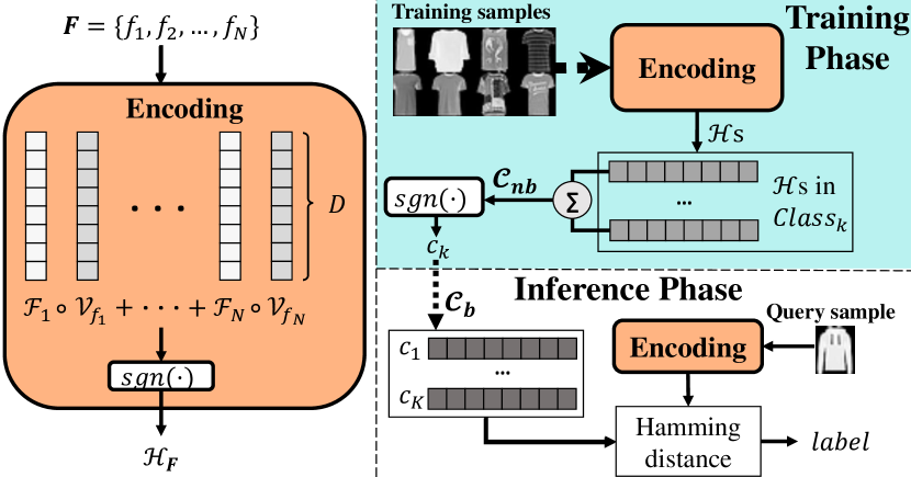
Figure 1. Binary HDC classification framework.

Training. The basic training strategy in HDC is to simply accumulate all the samples belonging to that class, in order to obtain the class hypervectors $\mathcal{C}$:

(2) $$c_{k}=sgn\left(\sum_{\mathcal{H}\in\Omega_{k}}\mathcal{H}\right)$$

where $c_{k}$ denotes the $k$-th class hypervector in $\mathcal{C}$, and $\Omega_{k}$ is the set of sample hypervectors belonging to class $k$.

Inference. A query sample is first encoded using Eq. 1. Then, the similarities, measured in terms of the Hamming distance between the query hypervector and class hypervectors in $\mathcal{C}$ are calculated. The most similar one, i.e., the class with the lowest Hamming distance, is labeled as the predicted class. For the ease of understanding the HDC flow, we show the scheme of binary HDC classification in Fig. 1. This procedure is similar to the nearest centroid classification in machine learning (Levner, 2005), which searches for an optimal centroid for each class.

2.2. Training Enhancement

Various training strategies have been proposed to increase accuracy. Here, we introduce a state-of-the-art approach: retraining (Imani et al., 2019a).

Eq. 2 gives the initial training results for class hypervectors. The retraining strategy (Imani et al., 2019a) further fine-tunes the initial class hypervectors, in which both non-binary and binary class hypervectors are used for the training. Specifically, the binary class hypervectors are utilized for validation and non-binary ones are used for updating. As shown in Fig. 2, in each retraining iteration, training samples are classified based on the current binary class hypervectors. If a training sample is misclassified, then the non-binary class hypervectors will be updated regarding to the encoded hypervector ($\mathcal{H}$):

(3) $$\begin{split}c_{nb}^{+}&=c_{nb}^{+}+\alpha\mathcal{H}\\ c_{nb}^{-}&=c_{nb}^{-}-\alpha\mathcal{H}\end{split}$$

where $c_{nb}^{+}$ and $c_{nb}^{-}$ are the correct and misclassified non-binary class hypervectors, respectively, and $\alpha$ is referred to as the learning rate. This retraining step intends to increase the influence of misclassified sample on the correct class while reducing it on the misclassified class. The retraining stops when the updating on class hypervectors is negligible.

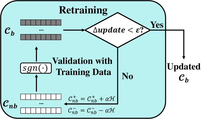
Figure 2. Retraining strategy to adjust class hypervectors against misclassified samples.

In addition, an ensemble approach (e.g., multi-model HDC where multiple models collectively classify each sample (Imani et al., 2019d)) can also increase the accuracy, but the storage size will grow when the number of ensembled HDC models increases.

3. Inner Mechanism of HDC Classifiers

In this section, we demonstrate the equivalence of a binary HDC classifier to a corresponding BNN for inference. Importantly, we highlight that the existing training strategies for HDC, are mostly heuristics and hence not optimal.

3.1. From Binary HDC to BNN

Considering a binary HDC classifier, we denote the input feature of a sample as $x\in\mathbb{R}^{N}$. The encoder in binary HDC will transfer the real-valued input feature $x$ to a binary hypervectors: $En(x):\mathbb{R}^{N}\mapsto\{-1,1\}^{D}$, where $D$ stands for the dimension of each hypervector, i.e., projecting the sample input from a low dimensional space to a much higher dimension. Assuming there are $K$ classes for this HDC classifier, a trained class hypervector set is $\mathcal{C}=\{c_{1},c_{2},...,c_{K}\}\in\{-1,1\}^{D\times K}$, where $c_{k}$ is the $k$-th class hypervector. The predicted label for the sample $x$ is

(4) $$k^{\star}=\underset{k}{argmin}\ Hamm(En(x),c_{k}),$$

where $Hamm(\mathcal{H}_{1},\mathcal{H}_{2})=\frac{|\mathcal{H}_{1}\neq\mathcal{H}_{2}|}{D}$ represents the normalized Hamming distance operator between any two hypervectors $\mathcal{H}_{1}$ and $\mathcal{H}_{2}$, and $|\mathcal{H}_{1}\neq\mathcal{H}_{2}|$ denotes the number of different bits in $\mathcal{H}_{1}$ and $\mathcal{H}_{2}$. A key property is that the hamming distance can be equivalently projected to the cosine similarity: $cosine(\mathcal{H}_{1},\mathcal{H}_{2})=1-2\cdot Hamm(\mathcal{H}_{1},\mathcal{H}_{2})$.

To see this point more concretely, we write the cosine similarity of two binary hypervectors $\mathcal{H}_{1}$ and $\mathcal{H}_{2}$ as

(5) $$\begin{split}cosine(\mathcal{H}_{1},\mathcal{H}_{2})=\frac{\mathcal{H}_{1}^{T}\mathcal{H}_{2}}{\|\mathcal{H}_{1}\|\ \|\mathcal{H}_{2}\|}\end{split}$$

where $\|\mathcal{H}_{1}\|$ and $\|\mathcal{H}_{2}\|$ denote the $l_{2}$ norms of $\mathcal{H}_{1}$ and $\mathcal{H}_{2}$, respectively. Due to the bipolar values $\{1,-1\}$ in hypervectors, we have $\mathcal{H}_{1}^{T}\mathcal{H}_{2}=(|\mathcal{H}_{1}=\mathcal{H}_{2}|-|\mathcal{H}_{1}\neq\mathcal{H}_{2}|)$. Plus the fact that $\|\mathcal{H}_{1}\|\ \|\mathcal{H}_{2}\|=D$ and $(|\mathcal{H}_{1}\neq\mathcal{H}_{2}|+|\mathcal{H}_{1}=\mathcal{H}_{2}|)=D$, we can conclude the equivalence between the Hamming distance and cosine similarity.

Therefore, the predicted label $k^{\star}$ can be equivalently represented as

(6) $$\begin{split}k^{\star}&=\underset{k}{argmin}\ Hamm(En(x),c_{k})\\ &=\underset{k}{argmax}\ cosine(En(x),c_{k})\\ &=\underset{k}{argmax}\ En(x)^{T}c_{k}\end{split}$$

Remark. From Eq. 6, we argue that the computation $\ En(x)^{T}c_{k}$ is actually the same as forward propagation in a BNN. Specifically, as illustrated in Fig. 4, the single-layer BNN takes $En(x)$ as its input and has $K$ output neurons that represent $K$ classes. The binary connection weights between the input $En(x)\in\{-1,1\}^{D}$ and the $k$-th output neuron is $c_{k}\in\{-1,1\}^{D}$, while the $k$-th output is $\ En(x)^{T}c_{k}$ and non-binary.

While binary HDC is the mainstream choice for HDC classifiers, our analysis also applies to non-binary HDC, where the encoded hypervector $En(x)$ and class hypervector $c_{k}$ can take both non-binary values. In this case, cosine similarity is directly used as the measure between $En(x)$ and $c_{k}$ for classification, and a non-binary HDC can be equivalently viewed as a simple single-layer neural network (i.e., perceptron).

3.2. Limitations in Current HDC Training

By establishing the equivalence between a binary HDC model and a BNN, we can see that the HDC training process (i.e., finding class hypervectors $\{c_{1},\cdots,c_{K}\}$) is essentially the same as training the BNN weights $c_{1},\cdots,c_{K}$.

In the basic HDC training process, each class hypervector $c_{k}$ is obtained by simply averaging the sample hypervectors $En(x)$ of all the samples belonging to that class. Clearly, this naive approach does not optimize the BNN weight $c_{k}$ at all. Next, we also highlight the key limitations in the state-of-the-art retraining strategy.

(1) Retraining only updates non-binary class hypervectors that correspond to the misclassified class and the true class, while other class hypervectors stay the unchanged. Intuitively, when a training sample $x$ is misclassified, the retraining step can partially mitigate the impact of $En(x)$ on the misclassified class hypervector while enhancing its impact on the true one; when a training sample is correctly classified, no action is taken. However, this strategy neglects two scenarios that could occur during the retraining phase: If a training sample $x$ is misclassified, while there are multiple wrong labels with high similarity, only the class hypervector corresponding to the wrong label with the highest similarity is updated. Hence, other wrong class hypervectors can only be updated in the future iterations, or even never get updated. If a training sample $x$ is correctly classified, even though the correct label has a slightly higher similarity than other classes (i.e., the other class hypervectors also have high similarities to this sample), no class hypervectors are updated. In this case, albeit correctly classified, this sample is very close to the classification border. If more samples of this kind occur during the training process, over-fitting is likely to happen, thus weakening the generalization of the HDC model. In contrast, there are various mechanisms, such as dropout and regularization, which mitigate the over-fitting in BNNs. Thus, by training the equivalent BNN, we can systematically improve the testing accuracy of HDC models.

(2) All the weights along the updating class hypervector have to be updated with a fixed step size. In the retraining strategy (Imani et al., 2019a), the updating scale is only determined by the encoded hypervector $En(x)$ and a fixed learning rate $\alpha$, as shown in Eq.3. On the other hand, the general updating rule for a (single-layer) DNN is:

(7) $$c^{t+1}_{k,j}=c^{t}_{k,j}-\alpha\frac{\partial\mathcal{L}}{\partial c_{k,j}}x$$

where $c_{k,j}^{t}$ is one weight parameter for iteration $t$, $\mathcal{L}$ denotes the loss function, $\alpha$ is the learning rate, and $x$ stands for the sample input equivalent to $En(x)$ in the HDC model. By comparing Eq.3 and Eq.7, we can directly observe that the derivative of the error $\frac{\partial\mathcal{L}}{\partial c_{i,j}}$ is overlooked in the retraining strategy. For this single-layer network, the derivative of loss function can reflect the similarity between the input $En(x)$ and the class hypervectors $c_{k},k\in\{1,2,...,K\}$. However, the retraining strategy indeed does not consider the similarity during the updating. As an improved version, adaptive learning rate is proposed in (Imani et al., 2019c), but the adaptability is still determined on the validation error rate or the difference between the similarities of $cosine(En(x),c_{correct})$ and $cosine(En(x),c_{wrong})$, not the similarities themselves on all class hypervectors. Consequently, the state-of-the-art retraining strategy will converge very slowly due to updating with incomplete information.

3.3. Case Study

We now practically demonstrate how thes limitations can affect HDC training. For the case study, we use Fashion-MNIST dataset (Xiao et al., 2017) to illustrate the inner mechanism of HDC learning. Fashion-MNIST consists of $L=60,000$ training images which are classified into $K=10$ classes, and we set the hypervector dimension as $D=10,000$.

In Fig. 3, we compare the performance of enhanced retraining against that of the default retraining. We make modifications on top of the existing retraining strategy to enhance the retraining process. Specifically, once a training sample is misclassified, all the class hypervectors that have higher similarities than the correct class hypervector will be updated, instead of only the one with the highest similarity. During the updating, we add the similarity influence. We specify that the ideal Hamming distance between the training sample and the correct/wrong class hypervector is 0/0.5. Then, we calculate the difference between the Hamming distance and the ideal one, and use it as a scaling factor for updating a class hypervector during retraining. This is equivalent to Eq. 7 when the loss function is the squared error.

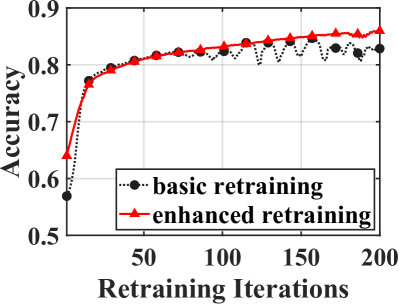
(a) Training trajectory

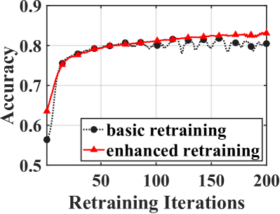
(b) Testing trajectory

Figure 3. Iteration comparison on the basic (Imani et al., 2019a) and the enhanced retraining strategy. The enhanced method adds similarity consideration and multiple updates during retraining.

The result shows that, for both the training and testing procedures, the enhanced retraining strategy can start with and converge at a higher accuracy, affirming that the discussed limitations indeed limit the retraining strategy. On the other hand, the basic retraining strategy starts to oscillate after the initial convergence. In contrast, the enhanced retraining can make the training/testing procedure more stable, due to the introduction of similarity metric for scaling the updating steps. Nonetheless, the enhancements we make are still heuristic, lacking principled guidance to optimize the class hypervectors in HDC.

4. LeHDC: the Learning-Based HDC

We now present LeHDC as an alternative and principled approach to train the class hypervectors in an HDC classifier. Based on the discovered equivalence between an HDC model and a single-layer BNN, LeHDC leverages state-of-the-art principled learning algorithms to train the BNN weights.

Compared to non-binary neural networks, BNN is more challenging to train, as the weights and output values are all binary. For instance, a large learning rate may successfully flip the binary weights but introduce severe oscillation at the same time; while a small learning rate may not be powerful enough to flip binary bits, resulting in the updating trapped in local optima. A BNN model for the binary HDC learning is demonstrated in Fig. 4. Here, $En(x)$ is an encoded sample hypervector and the input to the BNN, $\mathcal{C}$ represents the class hypervectors and are the BNN weights, and output o is $(En(x)^{T}c_{1},\cdots,En(x)^{T}c_{K})$ and equivalently measures the similarities between the input and each class. In this paper, we adopt the state-of-the-art BNN training strategy in (Liu et al., 2021), and propose the following approach to obtaining the optimal class hypervectors.

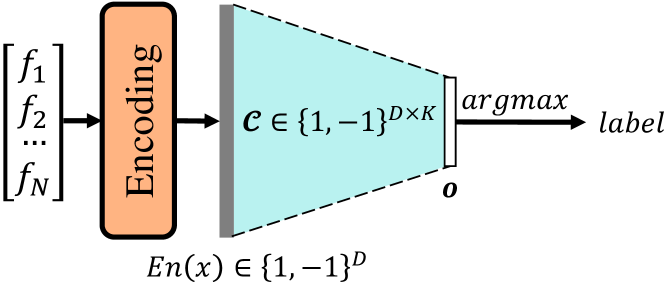
Figure 4. The equivalent BNN model for binary HDC.

Unlike other BNN models, our single-layer BNN corresponding to the binary HDC model does not require the binary activation function at each output neuron, since the non-binary BNN outputs (i.e., $\ En(x)^{T}c_{k}$, for $k=1,\cdots,K$) are directly used to determine the classification result. For the binary weights $\mathcal{C}\in\{-1,1\}^{D\times K}$ (i.e., class hypervectors), both binary ($\mathcal{C}$) and non-binary ($\mathcal{C}_{nb}$) forms are stored during training. The non-binary hypervectors are utilized to accumulate small gradients, and they are updated during the back propagation. The binary hypervectors are utilized for feed-forward and updated after each iteration as:

(8) $$\mathcal{C}=sgn(\mathcal{C}_{nb})=\begin{cases}-1\ \ \text{if $\mathcal{C}_{nb}$ < 0}\\ +1\ \ \text{otherwise.}\end{cases}$$

For each sample $x$, the true label ${y}$ is one-hot encoded at the output layer. During the training, the softmax function is applied to the output, and the cross entropy is used as the training loss function. Thus, the loss function of the output $\textbf{o}=En(\mathbf{X})\times\mathcal{C}$ can be denoted as

(9) $$\text{Loss}=\text{CrossEntropy}(\text{softmax}(\textbf{o}),{y})$$

Besides, weight decay is also an important step in BNN training. Weight decay usually behaves as a $L2$-norm penalty to prevent the weights from evolving too large, which is an effective strategy to mitigate over-fitting during the training. Combined with small gradients accumulated on non-binary class hypervectors, weight decay makes $\mathcal{C}_{nb}$ more sensitive to the input patterns and less dependent on the weight initialization. Hence, the final empirical loss is given as

(10) $$\mathcal{L}=\sum_{i}\text{CrossEntropy}(\text{softmax}(En({x}_{i})^{T}\mathcal{C}),{y}_{i})+\frac{\lambda}{2}\left\|\mathcal{C}_{nb}\right\|^{2}$$

where $({x}_{i},y_{i})$ is the training sample $i$ and $\lambda$ is a regularization weight. As the training configuration, $Adam$ is selected as the optimizer. Regarding the evaluations in (Liu et al., 2021), $Adam$ can outperform other $SGD$-based algorithms on the BNN optimization.

Moreover, the dropout strategy also plays an indispensable role in the equivalent single-layer BNN training. Since updating all weights is likely to introduces over-fitting, dropout is proposed to greatly prevent the over-fitting (Srivastava, 2013). Here, despite that LeHDC only has one layer without a complex architecture, its width is large and all the $D$ values corresponding to each class hypervector are straightforwardly updated, based on the gradient of loss. This may force the class hypervectors adapt to the training samples, leading to over-fitting. Hence, dropout is necessary to obtain the better performance on the HDC classification.

With the equivalent BNN model, we propose LeHDC for binary HDC classification. Our training method solves the mentioned limitations in current HDC training strategies and mitigates the over-fitting issue in a principled manner, providing better generalization ability. The cross entropy function along with the weight decay and dropout strategies are only used for training the equivalent BNN. After training, the weight matrix $\mathcal{C}=sgn(\mathcal{C}_{nb})$ can be directly used as the class hypervectors. The HDC inference process remains the unchanged, without requiring extra resources. Hence, LeHDC induces zero resource and time overhead during inference. Further, our method is inspired by modern BNN training techniques, which have theoretical support to approach the optimum of HDC training, rather than using heuristic training strategies in the existing HDC models.

Table 1. Inference accuracy (%) comparison between LeHDC and other strategies. Data are shown with format $mean^{\pm std}$.

	MNIST	Fashion-MNIST	CIFAR-10	UCIHAR	ISOLET	PAMAP	Avg Increment
Baseline Binary HDC	$80.36^{\pm 0.11}$	$68.04^{\pm 0.17}$	$29.55^{\pm 0.35}$	$82.46^{\pm 0.11}$	$87.42^{\pm 0.15}$	$77.66^{\pm 0.01}$	$-$
Multi-Model (Imani et al., 2019d)	$84.43^{\pm 0.5}$	$74.05^{\pm 0.5}$	$22.66^{\pm 0.59}$	$82.31^{\pm 0.89}$	$83.47^{\pm 0.43}$	$91.87^{\pm 0.85}$	$+2.22$
Retraining (Imani et al., 2019a)	$89.28^{\pm 0.07}$	$80.26^{\pm 0.27}$	$28.42^{\pm 1.46}$	$91.25^{\pm 0.21}$	$92.70^{\pm 0.12}$	$95.64^{\pm 0.03}$	$+8.67$
LeHDC	$\mathbf{94.74^{\pm 0.18}}$	$\mathbf{87.11^{\pm 0.08}}$	$\mathbf{46.10^{\pm 0.20}}$	$\mathbf{95.23^{\pm 0.16}}$	$\mathbf{94.89^{\pm 0.17}}$	$\mathbf{99.55^{\pm 0.05}}$	+15.32

5. Experiments

We evaluate the proposed LeHDC on several selected benchmarks: CV classification tasks (MNIST (Lecun et al., 1998), Fashion-MNIST (Xiao et al., 2017), and CIFAR-10 (Krizhevsky et al., 2009)) and datasets used in the original retraining work (Imani et al., 2019a) (UCIHAR (Anguita et al., 2013), ISOLET (Dua and Graff, 2017), and PAMAP (Reiss and Stricker, 2012)). Our goal is to highlight the advantages of LeHDC over the existing HDC training processes, and hence we mainly compare LeHDC against the existing HDC models. Note that the pros and cons between a general HDC and conventional machine learning models have been extensively studied in the literature, which is thus not the focus in this work (Imani et al., 2019b).

Unless otherwise stated, we adopt the follow configurations in our evaluation. For the retraining strategy, the learning rate is $\alpha=0.05$, and $\alpha=1.5$ in the first iteration. We run 150 iterations to ensure the retraining has converged. For the multi-model strategy, we follow the approach in (Imani et al., 2019d) and choose 64 hypervectors per class. For our proposed BNN-training strategy, the hyper-parameters are shown in Table 2. As a baseline reference, we test the benchmarks on binary HDC without any retraining. All the experiments are evaluated with Python on an 3.60GHz Intel i7-9700K CPU with 16GB memory and Tesla P100 GPU with 16GB memory.

5.1. Model Evaluation

First, we validate the significance of weight decay and dropout in LeHDC. In Fig. 5, we show the training and testing trajectories along the iterations on the CIFAR-10 dataset. By considering the weight decay and dropout during training, the testing accuracy can be increased. An interesting observation is that, if considering both the weight decay and dropout, the training accuracy will decrease. However, the testing accuracy in this case is the highest one. This is due to over-fitting that occurs when either weight decay or dropout is not included. Hence, the trained class hypervectors have better generality.

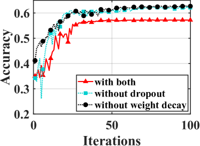
(a) Training trajectory

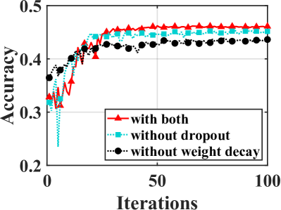
(b) Testing trajectory

Figure 5. The training and testing accuracy of CIFAR-10 along the iterations. We consider the cases that have weight decay, dropout, and both.

Further, we evaluate the scalability of LeHDC. We show the accuracy degradation along the dimension reduction across different training strategies in Fig. 6. We can see that LeHDC always outperforms other training strategies. Additionally, it achieves the same accuracy as $D=2,000$ as the retraining strategy with a much higher dimension $D=10,000$. Another observation is that the multi-model strategy sometimes may even perform worse than the baseline binary HDC, such as on the ISOLET dataset.

(a) Fashion-MNIST

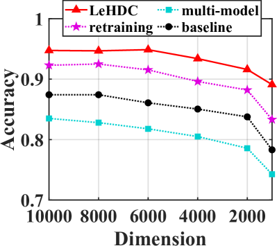
(b) ISOLET

Figure 6. The change of inference accuracy along with the dimension reduction on Fashion-MNIST and ISOLET datasets.

Moreover, we discuss the computational resource required for different binary HDC frameworks. Since LeHDC only optimizes the training procedure, without inducing extra computation during inference, it has the same time consumption and resource occupation as the baseline and retraining binary HDC. However, multi-model strategy costs more storage due to the multiple class hypervectors. Also, hardware acceleration on FPGA and in-memory computing is explored to support the inference in microseconds (Imani et al., 2019a, d). Thus, LeHDC improves the accuracy performance, with the same energy, latency, and size during inference.

5.2. Accuracy Improvement

We evaluate the accuracy performance of LeHDC with other HDC training strategies. We fine-tune the training configuration for each dataset, as shown in Table 2. Note that we still use $D=10,000$ for the evaluation, in order to make the comparison fair with other strategies. The learning rate will decay during the training, if the training loss increasing is detected.

Table 2. Hyper-parameters used in LeHDC configurations.

Dataset	Parameters
	WD1	LR2	B3	DR4	Epochs
MNIST	$0.05$	$0.01$	$64$	$0.5$	$100$
Fashion-MNIST	$0.03$	$0.1$	$256$	$0.3$	$200$
CIAFR-10	$0.03$	$0.001$	$512$	$0.3$	$200$
UCIHAR, ISOLET, PAMAP	$0.05$	$0.01$	$64$	$0.5$	$100$
1WD = Weight Decay 2LR = Learning Rate 3B = Batch Size 4DR = Dropout Rate

The inference accuracy comparison is shown in Table 1. As shown in the results, baseline HDC performs the worst in most benchmarks. However, the multi-model strategy sometimes even performs worse than the baseline HDC, such as on the CIFAR-10 and ISOLET datasets. By observing the characteristic of these benchmarks, we find that these two datasets have a large number of features or classes, but relatively fewer training samples; thus, the multi-model cannot deal with a complicated HDC classification task without sufficient training samples. Meanwhile, the retraining strategy enhances the training procedure, and has good accuracy improvement against the baseline HDC. On the other hand, our proposed LeHDC further improves the inference accuracy against the retraining. Hence, LeHDC can make the HDC classification closer to an optimum with zero resource and time overhead during inference.

6. Conclusion and Discussion

In this work, we investigate the existing limitations in current HDC training strategies and construct an equivalent BNN to the binary HDC model. Accordingly, we propose LeHDC to train the class hypervectors on the BNN structure in a principled manner. The evaluation shows that the learning-based BNN strategy can outperform other HDC training strategies, achieving the best close-to-optimal accuracy performance out, while introducing zero resource and time overhead during the HDC inference.

Despite that we only fine-tune the explicit hyper-parameters, the LeHDC strategy outperforms other training strategies on the selected benchmarks. However, we note there are other implicit ones, such as the ratio of validation set and the learning rate decay along the training. Moreover, since HDC model can be equivalently represented as neural network models, along with the advances in training BNNs, we expect that the HDC model performance can be further improved by training an equivalent BNN.

Although significantly improving the inference accuracy with the same energy consumption and latency, we admit that the HDC-based inference is still not as powerful as modern DNN framework. For example, a Convolutional Neural Network (CNN) can easily achieve over 90% accuracy on CIFAR-10. This is mainly due to the fundamental limitations of the existing HDC framework, which is essentially a simple single-layer BNN.

References

- (1)
- Anguita et al. (2013) Davide Anguita, Alessandro Ghio, Luca Oneto, Xavier Parra, and Jorge Luis Reyes-Ortiz. 2013. A public domain dataset for human activity recognition using smartphones.. In Esann, Vol. 3. 3.
- Dua and Graff (2017) Dheeru Dua and Casey Graff. 2017. UCI Machine Learning Repository. http://archive.ics.uci.edu/ml
- Ge and Parhi (2020) Lulu Ge and Keshab K Parhi. 2020. Classification using hyperdimensional computing: A review. IEEE Circuits and Systems Magazine 20, 2 (2020), 30–47.
- Imani et al. (2019a) Mohsen Imani, Samuel Bosch, Sohum Datta, Sharadhi Ramakrishna, Sahand Salamat, Jan M Rabaey, and Tajana Rosing. 2019a. QuantHD: A quantization framework for hyperdimensional computing. IEEE Transactions on Computer-Aided Design of Integrated Circuits and Systems (2019).
- Imani et al. (2019b) Mohsen Imani, Yeseong Kim, Sadegh Riazi, John Messerly, Patric Liu, Farinaz Koushanfar, and Tajana Rosing. 2019b. A framework for collaborative learning in secure high-dimensional space. In 2019 IEEE 12th International Conference on Cloud Computing (CLOUD). IEEE, 435–446.
- Imani et al. (2019c) Mohsen Imani, Justin Morris, Samuel Bosch, Helen Shu, Giovanni De Micheli, and Tajana Rosing. 2019c. Adapthd: Adaptive efficient training for brain-inspired hyperdimensional computing. In 2019 IEEE Biomedical Circuits and Systems Conference (BioCAS). IEEE, 1–4.
- Imani et al. (2018) Mohsen Imani, Tarek Nassar, Abbas Rahimi, and Tajana Rosing. 2018. Hdna: Energy-efficient dna sequencing using hyperdimensional computing. In 2018 IEEE EMBS International Conference on Biomedical & Health Informatics (BHI). IEEE, 271–274.
- Imani et al. (2019d) Mohsen Imani, Xunzhao Yin, John Messerly, Saransh Gupta, Michael Niemier, Xiaobo Sharon Hu, and Tajana Rosing. 2019d. Searchd: A memory-centric hyperdimensional computing with stochastic training. IEEE Transactions on Computer-Aided Design of Integrated Circuits and Systems 39, 10 (2019), 2422–2433.
- Kanerva (2009) Pentti Kanerva. 2009. Hyperdimensional computing: An introduction to computing in distributed representation with high-dimensional random vectors. Cognitive computation 1, 2 (2009), 139–159.
- Karunaratne et al. (2020) Geethan Karunaratne, Manuel Le Gallo, Giovanni Cherubini, Luca Benini, Abbas Rahimi, and Abu Sebastian. 2020. In-memory hyperdimensional computing. Nature Electronics (2020), 1–11.
- Kim et al. (2020) Yeseong Kim, Mohsen Imani, Niema Moshiri, and Tajana Rosing. 2020. GenieHD: Efficient DNA pattern matching accelerator using hyperdimensional computing. In 2020 Design, Automation & Test in Europe Conference & Exhibition (DATE). IEEE, 115–120.
- Krizhevsky et al. (2009) Alex Krizhevsky, Geoffrey Hinton, et al. 2009. Learning multiple layers of features from tiny images. (2009).
- Lecun et al. (1998) Y. Lecun, L. Bottou, Y. Bengio, and P. Haffner. 1998. Gradient-based learning applied to document recognition. Proc. IEEE 86, 11 (1998), 2278–2324. https://doi.org/10.1109/5.726791
- Levner (2005) Ilya Levner. 2005. Feature selection and nearest centroid classification for protein mass spectrometry. BMC bioinformatics 6, 1 (2005), 1–14.
- Liu et al. (2021) Zechun Liu, Zhiqiang Shen, Shichao Li, Koen Helwegen, Dong Huang, and Kwang-Ting Cheng. 2021. How Do Adam and Training Strategies Help BNNs Optimization? arXiv preprint arXiv:2106.11309 (2021).
- Reiss and Stricker (2012) Attila Reiss and Didier Stricker. 2012. Introducing a new benchmarked dataset for activity monitoring. In 2012 16th international symposium on wearable computers. IEEE, 108–109.
- Srivastava (2013) Nitish Srivastava. 2013. Improving neural networks with dropout. University of Toronto 182, 566 (2013), 7.
- Thapa et al. (2021) Rahul Thapa, Bikal Lamichhane, Dongning Ma, and Xun Jiao. 2021. SpamHD: Memory-Efficient Text Spam Detection using Brain-Inspired Hyperdimensional Computing. In 2021 IEEE Computer Society Annual Symposium on VLSI (ISVLSI). IEEE, 84–89.
- Xiao et al. (2017) Han Xiao, Kashif Rasul, and Roland Vollgraf. 2017. Fashion-MNIST: a Novel Image Dataset for Benchmarking Machine Learning Algorithms. arXiv:cs.LG/1708.07747 [cs.LG]
- Yu et al. (2022) Tao Yu, Yichi Zhang, Zhiru Zhang, and Christopher De Sa. 2022. Understanding Hyperdimensional Computing for Parallel Single-Pass Learning. arXiv preprint arXiv:2202.04805 (2022).