Fast Bayesian Coresets via Subsampling and Quasi-Newton Refinement

Abstract

Bayesian coresets approximate a posterior distribution by building a small weighted subset of the data points. Any inference procedure that is too computationally expensive to be run on the full posterior can instead be run inexpensively on the coreset, with results that approximate those on the full data. However, current approaches are limited by either a significant run-time or the need for the user to specify a low-cost approximation to the full posterior. We propose a Bayesian coreset construction algorithm that first selects a uniformly random subset of data, and then optimizes the weights using a novel quasi-Newton method. Our algorithm is a simple to implement, black-box method, that does not require the user to specify a low-cost posterior approximation. It is the first to come with a general high-probability bound on the KL divergence of the output coreset posterior. Experiments demonstrate that our method provides significant improvements in coreset quality against alternatives with comparable construction times, with far less storage cost and user input required.

1 Introduction

Bayesian methods are key tools for parameter estimation and uncertainty quantification, but exact inference is rarely possible for complex models. Currently, the gold standard method for approximate inference is Markov chain Monte Carlo (MCMC) [1; 2; 3, Ch. 11,12], which involves simulating a Markov chain whose stationary distribution is the Bayesian posterior. However, modern applications are often concerned with very large datasets; in this setting, MCMC methods typically have a $\Theta(NT)$ complexity—for $T$ samples and dataset size $N$ —which quickly becomes intractable as $N$ increases. Motivated by stochastic methods in variational inference [4, 5], this cost can be reduced by involving only a random subsample of $M\ll N$ data points in each Markov chain iteration [6, 7, 8, 9, 10, 11, 12, 13]. This reduces the per-iteration computation time of MCMC, but it can create substantial error in the stationary distribution of the resulting Markov chain and cause slow mixing [14, 15, 16, 11, 17].

Bayesian coresets [18, 19, 20, 21, 22, 23] provide an alternative for reducing the cost of MCMC and other inference methods. The key idea is that in a large-scale data setting, much of the data is often redundant. In particular, there often exists a fixed small, weighted subset of the data—a coreset—that suffices to capture the dataset as a whole in some sense [21]. Thus, if one can find such a coreset, it can be used in place of the full dataset in the MCMC algorithm, providing the simplicity, generality, and per-iteration speed of data-subsampled MCMC without the statistical drawbacks. Current state-of-the-art Bayesian coreset approaches based on sparse variational inference [21] empirically provide high-quality coresets, but are limited by their significant run-time and lack of theoretical convergence guarantees. Methods based on sparse regression [19, 20, 23] are significantly faster and come with some limited theoretical guarantees, but require a low-cost approximation to the full posterior. This approximation is often impractical to find and difficult to tune. Moreover, it can fundamentally limit the quality of the coreset obtained. Aside from [21], these methods also require $\Theta(N)$ storage, which is problematic in the large-data setting. There is a third class of constructions based on importance sampling [18], but these do not provide reliable posterior approximations in practice.

In this work, we develop a novel coreset construction algorithm that is both faster and easier to tune than the current state of the art, and has theoretical guarantees on the quality of its output. The key insight in our work is that we can split the construction of a coreset into two stages: first we select the data in the coreset via uniform subsampling—an idea developed concurrently by [24, 25]—and then optimize the weights using a few steps of a novel quasi-Newton method. Selecting points uniformly randomly avoids the slow inner-outer loop optimization of [21], and guarantees that the optimally-weighted coreset has a low KL divergence to the posterior (Theorems 4.1 and 4.2). Weighting these uniformly selected points correctly is crucial, and our quasi-Newton method is guaranteed to converge to a point close to the optimally-weighted coreset (Theorem 4.3) in significantly fewer iterations than the method of [21]. Finally, our method is easy to tune and does not require the low-cost posterior approximation of [19, 20]. Our experiments show that the algorithm exhibits significant improvements in coreset quality against alternatives with comparable construction times.

2 Bayesian coresets

The problem we study is as follows. Suppose we are given a target probability density $\pi(\theta)$ for variable $\theta\in\Theta$ that is comprised of $N$ potentials $\left(f_{n}(\theta)\right)_{n=1}^{N}$ and base density $\pi_{0}(\theta)$,

$$\pi(\theta)\coloneqq\frac{1}{Z}\exp\left(\sum_{n=1}^{N}f_{n}(\theta)\right)\pi_{0}(\theta),$$ (1)

where $Z$ is the normalizing constant. This setup corresponds to a Bayesian statistical model with prior $\pi_{0}$ and i.i.d. data $X_{n}$ conditioned on $\theta$, where $f_{n}(\theta)=\log p(X_{n}|\theta)$. Computing expectations under $\pi$ exactly is often intractable. MCMC methods can be employed here, but typically have a computational complexity of $\Theta(NT)$ to obtain $T$ samples, since $\sum_{n}f_{n}(\theta)$ needs to be evaluated at each step. Bayesian coresets [18] offer an alternative, by constructing a small, weighted subset of the dataset, on which any MCMC algorithm can then be run.

To do this, we find a set of weights $w\in\mathbb{R}_{\geq 0}^{N}$ corresponding to each data point, with the constraint that only $M\ll N$ of these are nonzero, i.e. $\left\lVert w\right\rVert_{0}\coloneqq\sum_{n=1}^{N}\mathds{1}_{w_{n}>0}\leq M.$ The weighted subset of points corresponding to the strictly positive weights is called a coreset, and we can then create the coreset posterior approximation,

$$\pi_{w}(\theta)\coloneqq\frac{1}{Z(w)}\exp\left(\sum_{n=1}^{N}w_{n}f_{n}(\theta)\right)\pi_{0}(\theta),$$ (2)

where $Z(w)$ is the new normalizing constant, and $\pi_{1}=\pi$ corresponds to the full posterior. Running MCMC on this approximation has complexity $\Theta(MT)$, a considerable speedup if $M\ll N$.

Constructing a sparse set of weights $w$ so that $\pi_{w}$ is as close to $\pi$ as possible is the key challenge here. Methods based on importance sampling [18] and sparse regression [19, 20, 23] have been developed, but these provide poor posterior approximations or require first finding a low-cost posterior approximation. The current state-of-the-art approach resolves both of the aforementioned issues by formulating the coreset construction problem as variational inference in the family of coresets [21]:

$$w^{\star}=\underset{w\in\mathbb{R}^{N}}{\arg\min}\quad\mathrm{D}_{\mathrm{KL}}\left(\pi_{w}\|\pi_{1}\right)\quad\text{s.t.}\quad w\geq 0,\|w\|_{0}\leq M,$$ (3)

where $\mathrm{D}_{\mathrm{KL}}(\cdot\|\cdot)$ denotes the KL divergence. Noting that coresets are a sparse subset of an exponential family—the weights form the natural parameter $w\in\mathbb{R}_{\geq 0}^{N}$, the component potentials $\left(f_{n}(\theta)\right)_{n=1}^{N}$ form the sufficient statistic, $\log Z(w)$ is the log partition function, and $\pi_{0}$ is the base density,

$$\pi_{w}(\theta):= \exp\left(w^{T}f(\theta)-\log Z(w)\right)\pi_{0}(\theta),\quad f(\theta):=(f_{1}(\theta),\dots,f_{N}(\theta))^{T}\in\mathbb{R}^{N},$$ (4)

one can obtain a formula for the gradient

$$\nabla_{w}\mathrm{D}_{\mathrm{KL}}\left(\pi_{w}\|\pi_{1}\right)= -\nabla_{w}^{2}\log Z(w)(1-w)=-\operatorname{Cov}_{w}\left[f,f^{T}(1-w)\right],$$ (5)

where $\operatorname{Cov}_{w}$ denotes covariance under $\pi_{w}$. Here, and throughout, we take derivatives with respect to $w$ on the ambient space $w\in\mathbb{R}^{N}$. The method of [21] then involves selecting a data point to add to the coreset, optimizing the coreset weights using stochastic gradient estimates based on Eq. 5, and then iterating. In practice, this method is infeasibly slow outside of small-data problems. For every data point selected it requires sampling from $\pi_{w}$ a number of times equal to the number of optimization steps (set to $100$ in [21]). This can easily lead to tens of thousands of sampling steps in total, each of which typically necessitates the use of an MCMC algorithm. Conversely, our method requires tens of sampling steps in total.

3 Construction via subsampling and quasi-Newton refinement

In this section, we provide a new Bayesian coreset construction algorithm (Algorithm 1) to solve the sparse variational inference problem Eq. 3. This method involves first uniformly subsampling the data, and then optimizing the weights on the subsample. Here, we give a detailed explanation of how the algorithm works. We defer to Section 4 the theoretical analysis of the method, which demonstrates that, with high probability, it finds a near-optimal coreset in a small number of optimization iterations.

3.1 Uniform subsampling

The first key insight to our approach is that we can select the $M$ data points that comprise the coreset by simple uniform subsampling. From an algorithmic standpoint, the benefit of this approach is clear: it makes the selection of coreset points fast and easy to implement. It also decouples the subset selection from the optimizing of the coreset weights, leaving us with a simpler optimization problem to solve. Intuitively, this is reasonable from a coreset quality standpoint because a uniform subsample of the data will, with high probability, create a highly-expressive “basis” of log-likelihood functions $\left(f_{n}\right)_{n=1}^{M}$ with which to approximate the full data log-likelihood. Of course, we still need to optimize the coreset weights; but we have not limited the flexibility of the coreset family significantly by selecting points via uniform subsampling. Theorem 4.2 provides a precise statement of these ideas, and shows that the optimal weighted coreset posterior built using a uniformly random subset of data is a good posterior approximation.

Since the coreset data points are chosen uniformly randomly, we will w.l.o.g. re-label the selected subset to have indices $1,\dots,M$, and the remaining data points to have indices $M+1,\dots,N$ from now on. We can specify a new weight constraint set $\mathcal{W}\subset\mathbb{R}^{N}$ of vectors $w$ with 0 entries for every index beyond $M$, and a further subset $\mathcal{W}_{N}$ where the weights sum to $N$,

$$\mathcal{W}=\left\{w\in\mathbb{R}^{N}:w\geq 0,\,\,n>M\implies w_{n}=0\right\},\qquad\mathcal{W}_{N}=\left\{w\in\mathcal{W}:1^{T}w=N\right\}.$$

It is also useful to denote $g(\theta)=(f_{1}(\theta),\dots,f_{M}(\theta))^{T}\in\mathbb{R}^{M}$ as the first $M$ components of $f(\theta)$.

3.2 Quasi-Newton optimization

Given the choice of $M$ data points to include in the coreset, it is crucial to optimize their weights correctly. This is the second step of our algorithm. The KL divergence gradient for the $M$ weights is

$$\nabla_{w}\mathrm{D}_{\mathrm{KL}}\left(\pi_{w}\|\pi_{1}\right)= \left(-\nabla_{w}^{2}\log Z(w)(1-w)\right)_{1:M}=-\operatorname{Cov}_{w}\left[g,f^{T}(1-w)\right].$$ (6)

To reduce the number of weight optimization iterations —each of which generally involves MCMC sampling from $\pi_{w}$, where $w$ is the current set of weights—we develop a second-order optimization method. Again using the properties of exponential families, we can derive the Hessian of the KL divergence with respect to the $M$ weights

$$\nabla^{2}_{w}\mathrm{D}_{\mathrm{KL}}\left(\pi_{w}\|\pi_{1}\right)=\left(\nabla_{w}^{2}\log Z(w)\!-\!\nabla^{3}_{w}\log Z(w)(1\!-\!w)\right)_{1:M,1:M}.$$

This matrix is not guaranteed to be positive (semi-)definite. However, writing out the second term explicitly as

$$\nabla_{w}^{3}\log Z(w)(1-w)=\mathbb{E}_{\pi_{w}}\left[\left(f-\mathbb{E}_{\pi_{w}}(f)\right)\left(f-\mathbb{E}_{\pi_{w}}(f)\right)^{T}\left((f^{T}(1-w)-\mathbb{E}_{\pi_{w}}(f^{T}(1-w))\right)\right],$$

we see that this term will be small near the optimum, where the coreset approximation is ideally good, i.e., $w^{T}f(\theta)\approx 1^{T}f(\theta)$. The first term does not contain this $f^{T}(1-w)$ term, and thus should dominate the expression.

This motivates the use of

$$\nabla^{2}_{w}\mathrm{D}_{\mathrm{KL}}\left(\pi_{w}\|\pi_{1}\right)\approx\left(\nabla_{w}^{2}\log Z(w)\right)_{1:M,1:M}=\operatorname{Cov}_{w}\left[g,g\right]$$ (7)

to scale gradient steps in the optimization method rather than the true Hessian, thus creating a quasi-Newton method [26]. This heuristic motivates our approach, but it is rigorously justified by Theorem 4.3, which proves that this scaling results in optimization iterations that are guaranteed to converge exponentially to a coreset which is nearly globally optimal. Note that when $M$ is larger than the inherent dimension of the space of log-likelihood functions, $\operatorname{Cov}_{w}\left[g,g\right]$ will have zero eigenvalues and be noninvertible. Therefore we add a regularization $\tau>0$ prior to inversion. Theorem 4.3 shows how the regularization influences the optimization, but in general we want $\tau$ to be as small as possible while still ensuring the numerical stability of inverting $\operatorname{Cov}_{w}\left[g,g\right]$.

Our optimization method is as follows. First, we initialize at the uniformly weighted coreset, i.e.,

$$w_{0}\in\mathcal{W},\quad w_{0m}=\frac{N}{M},\quad m=1,\dots,M.$$

Next, given a step-size tuning sequence $\gamma_{k}$, $k\geq 0$, we update the weights at each iteration $k\in\mathbb{N}\cup\{0\}$ using the $(\tau>0)$-regularized quasi-Newton step

$$\hat{w}_{k+1} =w_{k}+\gamma_{k}(G(w_{k})+\tau I)^{-1}H(w_{k})(1-w_{k})$$ (8)

$$G(w) =\mathrm{Cov}_{w}\left[g,g\right],\quad H(w)=\mathrm{Cov}_{w}\left[g,f\right].$$ (9)

Theorem 4.3 suggests that the step size $\gamma_{k}$ should be constant: $\gamma_{k}=\gamma\in(0,1]$; but the analysis in that section assumes that we can compute $G(w)$ and $H(w)$ exactly, whereas in practice we will have to estimate them. Hence we allow $\gamma_{k}$ to depend on the iteration number in general. Finally, we project $\hat{w}_{k+1}$ back onto the constraint set to obtain next iterate $w_{k+1}$, i.e. for $m=1,\ldots,M$ set

$$w_{k+1,m}=\max\left(\hat{w}_{k+1,m},0\right).$$ (10)

3.3 Algorithm

The pseudocode for the quasi-Newton coreset construction method is shown in Algorithm 1. There are a number of practical considerations needed to use this method; we discuss these here.

The first consideration is that we cannot calculate $G(w)$ and $H(w)$ in closed form. Instead, at step $k$ of the algorithm, we use a Monte Carlo estimate; first taking $S$ samples $\left(\theta_{s}\right)_{s=1}^{S}\stackrel{{\scriptstyle\text{ i.i.d. }}}{{\sim}}\pi_{w_{k}}$, and calculating $\hat{g}_{s}:=g(\theta_{s})-\frac{1}{S}\sum_{r=1}^{S}g(\theta_{r})$, so that we may estimate $G(w_{k})$ as

$$\hat{G}_{k} =\frac{1}{S}\sum_{s=1}^{S}\hat{g}_{s}\hat{g}_{s}^{T}\,\,\in\mathbb{R}^{M\times M}.$$ (11)

Using a Monte Carlo estimate in this way introduces one source of error. Furthermore, we often cannot sample exactly from $\pi_{w_{k}}$, and instead use MCMC to do so. This could lead to additional errors, for example if our samples are from unconverged chains. However, we find that this method works well in practice, for a reasonable number of samples $S$.

As $H(w_{k})$ is an $M\times N$ matrix, estimating it directly will incur a $\Theta(MN)$ storage cost. Instead, we note that we only require $H(w_{k})(1-w_{k})=\mathrm{Cov}_{w_{k}}\left[g,f^{T}(1-w_{k})\right]=\mathrm{Cov}_{w_{k}}\left[g,h\right]$, where $h\coloneqq f^{T}1-g^{T}w_{k}=\bar{f}-g^{T}w_{k}$. We can estimate $h$ using $\hat{h}_{s}=\sum_{n=1}^{N}\left[f_{n}(\theta_{s})-\frac{1}{S}\sum_{r=1}^{S}f_{n}(\theta_{r})\right]-\hat{g}_{s}^{T}w_{k}$, which requires $O(N)$ time, but only $O(S)$ space. We can then estimate $H(w_{k})(1-w_{k})$ as

$$\hat{H}_{k}(1-w_{k}) =\frac{1}{S}\sum_{s=1}^{S}\hat{g}_{s}\hat{h}_{s}.$$ (12)

Thus, we can find $w_{k+1}$ from $w_{k}$ by taking the stochastic Newton step

$$\hat{w}_{k+1}=w_{k}+\gamma_{k}\left(\hat{G}_{k}+\tau I\right)^{-1}\hat{H}_{k}(1-w_{k}),$$ (13)

and projecting onto the constraint set: $w_{k+1,m}=\hat{w}_{k+1,m}\mathds{1}_{\hat{w}_{k+1,m}\geq 0}$. We set the regularization parameter $\tau$ by examining the condition number of $\hat{G}_{k}+\tau I$ and keeping it below a reasonable value. We can tune $\gamma_{k}$ using a line search method. As we do not have access to the objective function (i.e. the KL-divergence between the coreset and full posteriors), we use the curvature part of the Wolfe conditions [27] to tune this. In practice, this line search is expensive. Thus, we only tune $\gamma_{k}$ for $k\leq K_{\text{tune}}$, and leave it as a constant thereafter. The intuition here is that we may start with quite poor coreset weights, and so need to choose the initial steps carefully. In Appendix C, we perform a sensitivity analysis for the parameters $S$, $K_{tune}$ and $\tau$. We see that our results are generally not sensitive to the choice of these parameters, within reasonable ranges.

Algorithm 1 QNC (Quasi-Newton Coreset)

0:  $(f_{n}(\theta))_{n=1}^{N}$ $\pi_{0}$, $S$, $K$, $K_{tune}$, $\gamma$, $\tau$, $M$.

1:  Uniformly sample $M$ data points, w.l.o.g. these correspond to indices $1,\ldots,M$.

2:  Set $w_{0m}=\frac{N}{M},\quad m=1,\dots,M.$

3:  for $k=0,\ldots,K-1$ do

4:     Sample $\left(\theta_{s}\right)_{s=1}^{S}\stackrel{{\scriptstyle\text{ i.i.d. }}}{{\sim}}\pi_{w_{k}}\propto\exp\left(w_{k}^{T}f(\theta)\right)\pi_{0}(\theta)$

5:     Set $\hat{g}_{s}\leftarrow g(\theta_{s})-\frac{1}{S}\sum_{r=1}^{S}g(\theta_{r})$ and $\hat{h}_{s}\leftarrow\sum_{n=1}^{N}\left[f_{n}(\theta_{s})-\frac{1}{S}\sum_{r=1}^{S}f_{n}(\theta_{r})\right]-\hat{g}_{s}^{T}w_{k}$

6:     Set $\hat{H}_{k}(1-w_{k})\leftarrow\frac{1}{S}\sum_{s=1}^{S}\hat{g}_{s}\hat{h}_{s}$ and $\hat{G}_{k}\leftarrow\frac{1}{S}\sum_{s=1}^{S}\hat{g}_{s}\hat{g}_{s}^{T}$

7:     if $k\leq K_{\text{tune}}$ then

8:        Choose $\gamma_{k}$ via line search with starting value $\gamma$

9:     else

10:        Set $\gamma_{k}\leftarrow\gamma$

11:     Take a quasi-Newton step: $\hat{w}_{k+1}\leftarrow w_{k}+\gamma_{k}\left(\hat{G}_{k}+\tau I\right)^{-1}\hat{H}_{k}(1-w_{k})$

12:     Project: for all $m\in[M]$, $w_{k+1,m}\leftarrow\max\left(\hat{w}_{k+1,m},0\right)$

13:  return $w=w_{K}$

Computing $\hat{G}_{k}+\tau I$ involves taking $S$ samples, forming the product $\hat{g}_{s}\hat{g}_{s}^{T}$, and then inverting the resulting matrix. Its time complexity is thus $O(SM^{2}+M^{3})$. Computing $\hat{H}(w_{k})(1-w_{k})$ similarly has complexity $O\left(SM+SN\right)$, and computing the product with $(\hat{G}_{k}+\tau I)^{-1}$ has complexity $O\left(M^{2}\right)$. For $K$ Newton steps in Algorithm 1, the overall time complexity is thus $O(K(M^{3}+SM^{2}+SN))$, which is linear in $N$. The space complexity is $O(M^{2})$ (to store $\hat{G}_{k}$), which is sublinear in $N$, unlike in [20, 23].

In theory, we can reduce the time complexity by using a further stochastic estimate of $\hat{H}_{k}(1-w_{k})$. In particular, we can instead calculate $\hat{h}_{s}$ only for indices in $\mathcal{I}\coloneqq\{1,\ldots,M\}\cup\mathcal{T}$, where $\mathcal{T}$ is a uniformly selected sample $\mathcal{T}\subseteq\{1,\ldots,N\}$. Calculating $\hat{H}(w_{k})(1-w_{k})$ using this subsampled vector $\hat{h}_{s,\mathcal{I}}$ then has complexity $O(SM+ST)$ in the worst case, where $T\coloneqq|\mathcal{T}|$. The overall time complexity is then $O(K(M^{3}+SM^{2}+ST))$, which is sublinear in $N$ if $T=o(N)$. This could give significant improvements in coreset construction time in the large-data regime. However, this approach requires further study, as we find that it leads to a degradation in the performance of our algorithm. We do not use it in our experiments.

The final practical consideration in the design of Algorithm 1 is that we cannot actually calculate the objective function that we are trying to minimize, namely the KL divergence $\mathrm{D}_{\mathrm{KL}}\left(\pi_{w}\|\pi_{1}\right)$ between the coreset and full posteriors. Thus, it may be hard to tell if the optimization is actually making progress. In practice, we monitor the norm of the gradient of the KL divergence (which we do have access to, as given by Eq. 6). We can terminate our algorithm early if we do not see a significant enough decrease in this measure.

4 Theoretical analysis

In this section we provide a theoretical analysis of the proposed method. We demonstrate (in Theorems 4.1 and 4.2) that the optimal coreset posterior built using a uniformly random subset of data is, with high probability, an exact or near-exact approximation of the true posterior. Second, we show (in Theorem 4.3) that the proposed optimization algorithm converges exponentially quickly to a point near the optimal coreset, thus realizing the guarantee in Theorem 4.2 in practice, and theoretically justifying our proposed algorithm. The assumptions required for our theory are somewhat technical. We give some intuition here on settings where they hold, but discuss this further in Appendix A. Proofs of all results may be found in Appendix B.

4.1 Subset selection via uniform subsampling

Theorem 4.1 and Theorem 4.2 provide a theoretical foundation for selection via uniform subsampling. Both recommend setting $M\gtrsim d\log N$, where $d$ is essentially the “dimension” of the span of the log-likelihood functions. Theorem 4.1 states that if the span of the log-likelihood functions is indeed finite-dimensional with dimension $d$—e.g., in a usual exponential family model—then with high probability, the optimal coreset using a uniformly random selection of $M$ points is exact. Theorem 4.2 extends this to the general setting where $\Theta\subseteq\mathbb{R}^{D}$, $N$ is large relative to $D$, and where we assume the posterior concentrates as $N\to\infty$. In particular, Theorem 4.2 states that with high probability, the optimal coreset using a uniformly random selection of $M$ data points provides low error.

In what follows, we assume that $f_{n}(\cdot)$ are i.i.d. from some true data-generating distribution $p$, and we define $\bar{f}(\cdot)=\mathbb{E}_{p}(f_{n}(\cdot))$. We also introduce the new notation $f(\cdot,\cdot)$, where we consider the potentials $f$ as functions of both $x$ and $\theta$. This enables us to make the data-dependence explicit when needed, i.e., $f_{n}(\cdot)=f(x_{n},\cdot)$; for instance, in the standard context of Bayesian inference $f_{n}(\cdot)=f(x_{n},\cdot)=\log p(x_{n}|\cdot)$, with $x_{n}\overset{\text{i.i.d.}}{\sim}p_{0}$ for $n\in[N]$.

Theorem 4.1.

Let $S_{0}$ be the vector space of functions on $\Theta$ spanned by $\{f(x,\cdot);x\in\mathcal{X}\}$. Assume that $S_{0}$ is finite dimensional, with dimension $d$. Let $\mu$ be any measure on $\Theta$ such that $S_{0}\subset L^{2}(\mu)$ and denote $r^{2}_{\mu}=\mathbb{E}_{\mu}\left(\mathbb{E}_{p}([f_{1}-\bar{f}]^{2})\right)$. For $\delta>0$ define

$$J(\delta)=\!\!\!\!\!\inf_{a\in S_{0};\|a\|=1}\!\!\!\Pr\left(\!\!\langle a,\!f_{1}\!-\!\bar{f}\rangle_{L^{2}(\mu)}\!>\!\frac{2r_{\mu}}{\sqrt{N\delta}}\right)\!.$$ (14)

Then for $\delta>0$ such that $J(\delta)+\delta<1$, a universal constant $C_{1}$, and $M\in\mathbb{N}$ such that

$$M\geq\frac{2d}{J(\delta)}\left(\log N+\log\left(\frac{4\delta}{J(\delta)}\right)+C_{1}\right),$$

we have that with probability $\geq 1-\delta-e^{-MJ(\delta)/4}$,

$$\min_{w\in\mathcal{W}_{N}}\mathrm{KL}(\pi_{w}||\pi) =0.$$

Note that the condition that $S_{0}$ has finite dimension $d<\infty$ is satisfied for all $d$-dimensional exponential families when $f_{n}(\theta)=\log p(x_{n}|\theta)$. Further, note that Theorem 4.1 still applies in situations where $d$ increases with $N$. To understand the behaviour of $J(\delta)$, we consider in Appendix A a full rank exponential family. We can show that, under certain conditions, $J(\delta)$ converges to a strictly positive value as $\delta N\to\infty$. In this case, we can set $\delta=\omega(1/N)$, such that with probability $\geq 1-\omega(1/N)$, we indeed have that $\min_{w\in\mathcal{W}_{N}}\mathrm{KL}(\pi_{w}||\pi)=0$ for $M\gtrsim d\log N$.

In the interest of obtaining a more general approximation result, we now consider the case where $S_{0}$ is infinite dimensional, but where we can find a finite-dimensional space $S_{1}$ which approximates $f_{n}(\theta)-\bar{f}(\theta)$ reasonably well. A typical setup where this is valid is when $\Theta\subseteq\mathbb{R}^{D}$, the posterior concentrates (as $N\to\infty$) at a point $\theta_{0}\in\Theta$ that maximizes $\bar{f}(\theta)$, and each $f_{n}(\cdot)$ is smooth near $\theta_{0}$ and globally well-behaved in some sense. Theorem 4.2 below states, roughly, that for a model satisfying these assumptions, $\min_{w\in\mathcal{W}_{N}}\mathrm{KL}(\pi_{w}||\pi)$ will be small with high probability. We give the exact conditions in Appendix A. Although they are perhaps strong, the result is still indicative of when a good posterior approximation is obtained by our method.

Intuitively, we require that $f(x,\theta)$ be differentiable, strongly concave in $\theta$, and “smooth enough”. Letting $\theta_{0}$ be the unique value such that $\bar{f}(\theta)\leq\bar{f}(\theta_{0})$ $\forall\theta\in\Theta$, we also require that we can split $f(x;\theta)$ into two parts,

$$f(x,\theta)=f^{(1)}(x,\theta)+f^{(2)}(x,\theta),$$

where the span of $\left\{f^{(1)}(x,\cdot)-f^{(1)}(x,\theta_{0}):x\in\mathcal{X}\right\}$ is a finite-dimensional vector space $S_{1}$. This split needs to be made such that $f^{(2)}$ is negligible, in the sense that $f(x,\theta)\approx f^{(1)}(x,\theta)$ locally around $\theta_{0}$. A usual case where these conditions hold is when $f(x;\theta)$ is $C^{3}$ in $\theta$. In this case, we can obtain $f^{(1)}(x;\theta)$ by a second-order Taylor expansion,

$$f^{(1)}(x;\theta)=f(x;\theta_{0})+(\theta-\theta_{0})^{T}\nabla_{\theta}f(x;\theta_{0})+(\theta-\theta_{0})^{T}\nabla^{2}f(x;\theta_{0})(\theta-\theta_{0})/2,$$

which has dimension bounded by $1+D+D(D+1)/2$. $f^{(2)}(x;\theta)$ is then the remainder term, which is indeed negligible around $\theta_{0}$ in the desired sense. In Appendix A, we provide further discussion on the conditions of Theorem 4.2. Recalling that a quantity is $o(1)$ as $N\to\infty$ if and only if it converges to 0, we can then state the result as follows.

Theorem 4.2.

Suppose the assumptions A1-A4 in Appendix A hold, and we set $M\gtrsim D(\log N+1)$. Then as $N\to\infty$, with probability at least $1-o(1)$, we have that

$$\min_{w\in\mathcal{W}_{N}}\mathrm{KL}(\pi_{w}||\pi) =o(1).$$

In the above example, we can examine the proof to obtain a bound on $\mathrm{KL}(\pi_{w}||\pi)$ of order $1/\sqrt{N}$ with probability converging to 1, showing that this result does indeed lead to a useful bound.

4.2 Quasi-Newton weight optimization

Theorems 4.1 and 4.2 guarantee the existence of a high-quality coreset, but do not provide any insight into whether it is possible to find it tractably. Theorem 4.3 addresses this remaining gap. In particular, intuitively, it asserts that as long as (1) the regularization parameter $\tau>0$ is nonzero but small enough that it does not interfere with the optimization (in particular, the minimum eigenvalue of $G(w)$ over the space), and (2) the optimal coreset is a good approximation to the full dataset (which is already guaranteed by Theorem 4.2), then the weights $w_{k}$ at iteration $k$ of the approximate Newton method converge exponentially to a point close to a global optimum. In the result below, let $G(w)$ and $H(w)$ be defined as in Eq. 9.

Theorem 4.3.

Let $W\subseteq\mathcal{W}$ be a closed convex set, $W^{\star}\subseteq\arg\!\min_{w\in W}\mathrm{KL}(\pi_{w}||\pi)$ be a maximal closed convex subset, and fix the regularization parameter $\tau>0$. Define

$$\xi=\inf_{w\in W}\min\left\{\frac{\lambda}{\lambda+\tau}:\lambda\in\mathrm{eigvals}\,G(w),\,\lambda>0\right\}.$$

Suppose $\exists$ $\epsilon\in[0,1)$ and $\delta\geq 0$ such that for all $w\in W$

$$\|\left(G(w)\!+\!\tau I\right)^{-1}H(w)(1\!-\!w^{\star})\|\leq\epsilon\|w\!-\!w^{\star}\|\!+\!\delta,$$ (15)

where $w^{\star}=\mathrm{proj}_{W^{\star}}(w)$. Then the $k^{\text{th}}$ iterate $w_{k}\in W$ and its projection $w^{\star}_{k}=\mathrm{proj}_{W^{\star}}(w_{k})$ of the projected Newton method defined in Section 3.2 by Eqs. 8, LABEL:, 9, LABEL: and 10, initialized at $w_{0}\in W$ with a fixed step size $\gamma\in[0,1]$ and regularization $\tau$ satisfies

$$\left\|w_{k}-w^{\star}_{k}\right\| \leq\eta^{k}\left\|w_{0}-w^{\star}_{0}\right\|+\gamma\delta\left(\frac{1-\eta^{k}}{1-\eta}\right),\qquad\eta=1-\gamma(\xi-\epsilon).$$

For this result to make sense, we require that $\eta\in[0,1]$. We have that $\eta\geq 0$, since $\gamma\in[0,1]$, $\epsilon\geq 0$ and $\xi\leq 1$ by definition. It may be the case that $\eta\geq 1$, in which case our result still holds, but is vacuous.

In order to use this result, the minimum positive eigenvalue of $G(w)$ for $w\in W\subseteq\mathcal{W}$ needs to be bounded, as does the error of the optimal coreset weights $w^{\star}$ in the sense of Eq. 15. A notable corollary of Theorem 4.3 occurs when there exists a $w^{\star}$ such that

$$\forall\theta\in\Theta,\quad\sum_{m=1}^{M}w^{\star}_{m}f_{m}(\theta) =\sum_{n}f_{n}(\theta),$$

i.e., the optimal coreset is identical to the true posterior distribution, as is guaranteed by Theorem 4.1. For any model where the conditions of Theorem 4.1 hold, such as any exponential family model, Eq. 15 holds with $\epsilon=\delta=0$. We can thus take $\gamma=1$ to find that

$$\left\|w_{k}-w^{\star}_{k}\right\| \leq(1-\xi)^{k}\left\|w_{0}-w^{\star}_{0}\right\|.$$

This provides some intuition on Theorem 4.3; as long as the optimal coreset posterior is a reasonable approximation to $\pi$, and we use a small regularization $\tau>0$ (such that $\xi\approx 1$), then we generally need only a small number of optimization steps to find the optimal coreset. The conditions of Theorem 4.1 are sufficient, but not necessary, for Eq. 15 to hold. We present further discussion in Appendix A.

We note that if $\xi=0$, then there is no convergence, even in the setting where Theorem 4.1 holds. However, it is important to emphasises that, for any given dataset, we are free to choose $\tau$. We can (and should) choose $\tau$ to be sufficiently small that $\xi$ is roughly $1$. In particular, this means setting $\tau$ significantly smaller than the minimum positive eigenvalue of $G(w)$.

5 Experiments

In this section, we compare our proposed quasi-Newton coreset (QNC) construction against existing constructions—uniform subsampling (UNIF), greedy iterative geodesic ascent (GIGA) [20] and iterative hard thresholding (IHT) [23]—as well as the Laplace approximation (LAP), which represents what one obtains by assuming posterior normality in the large-data setting. Experiments were performed on a machine with a 2.6GHz 6-Core Intel Core i7 processor, and 16GB memory; code is available at https://github.com/trevorcampbell/quasi-newton-coresets-experiments.

In each case, we use $S=500$ Monte Carlo samples during coreset construction. We compute error metrics using 1000 samples from each method’s approximate posterior. We also compare to the baseline of sampling from the full posterior (FULL) to establish a noise floor for the given comparison sample size of 1000. In the synthetic Gaussian experiment, which is the simplest one we consider, we see that sparse variational inference (SVI) [21] is prohibitively slow, taking $4.2\times 10^{3}$s to construct a coreset of size 1 (and scaling at best linearly with coreset size). Thus, we do not compare against it here. In Appendix C we run a smaller, lower dimensional, synthetic Gaussian experiment. Here, we compare against SVI, and confirm that it is prohibitively slow for the size of datasets that we consider.

For GIGA and IHT, we need to supply a low-cost approximation $\hat{\pi}$ to the posterior. To ensure these methods apply as generally as QNC and SVI, we use a uniformly sampled coreset approximation of size $M$ with weights $N/M$ (where $M$ is the same as the desired coreset size we are constructing). We also use these weights for UNIF. In Appendix C we provide additional results for GIGA and IHT with a Laplace approximation used for $\hat{\pi}$. This does not lead to a significant improvement, and we provide further discussion there.

Experiments are performed in settings standard in the Bayesian coresets literature, but with larger dataset sizes than those that could be considered previously. For each experiment we plot the approximate reverse KL divergence obtained by assuming posterior normality, and the build time. In Appendix C we provide comparisons on the additional metrics of relative mean and covariance error, forward KL divergence and per sample time to sample from the respective posteriors. For the experiments in Sections 5.2 and 5.3 with heavy tailed priors, we also compare using the maximum mean discrepancy [28] and kernel Stein discrepancy [29, 30], with inverse multi-quadratic (IMQ) kernel.

Throughout the experiments, we see that QNC outperforms the other subsampling methods for most coreset sizes we consider. GIGA and IHT in particular are limited by a fixed choice of $\hat{\pi}$ and finite projection dimension defined by our choice of $S=500$—we discuss this further in Appendix C. Furthermore, outside of the synthetic Gaussian experiment, we see that QNC outperforms LAP for coreset sizes above certain thresholds, which represent a small fraction of the full dataset.

In Appendix C, we also perform a sensitivity analysis for the parameters $S$, $K_{tune}$ and $\tau$ that we use in Algorithm 1. We see that our results are generally not sensitive to the choice of these parameters, within reasonable ranges.

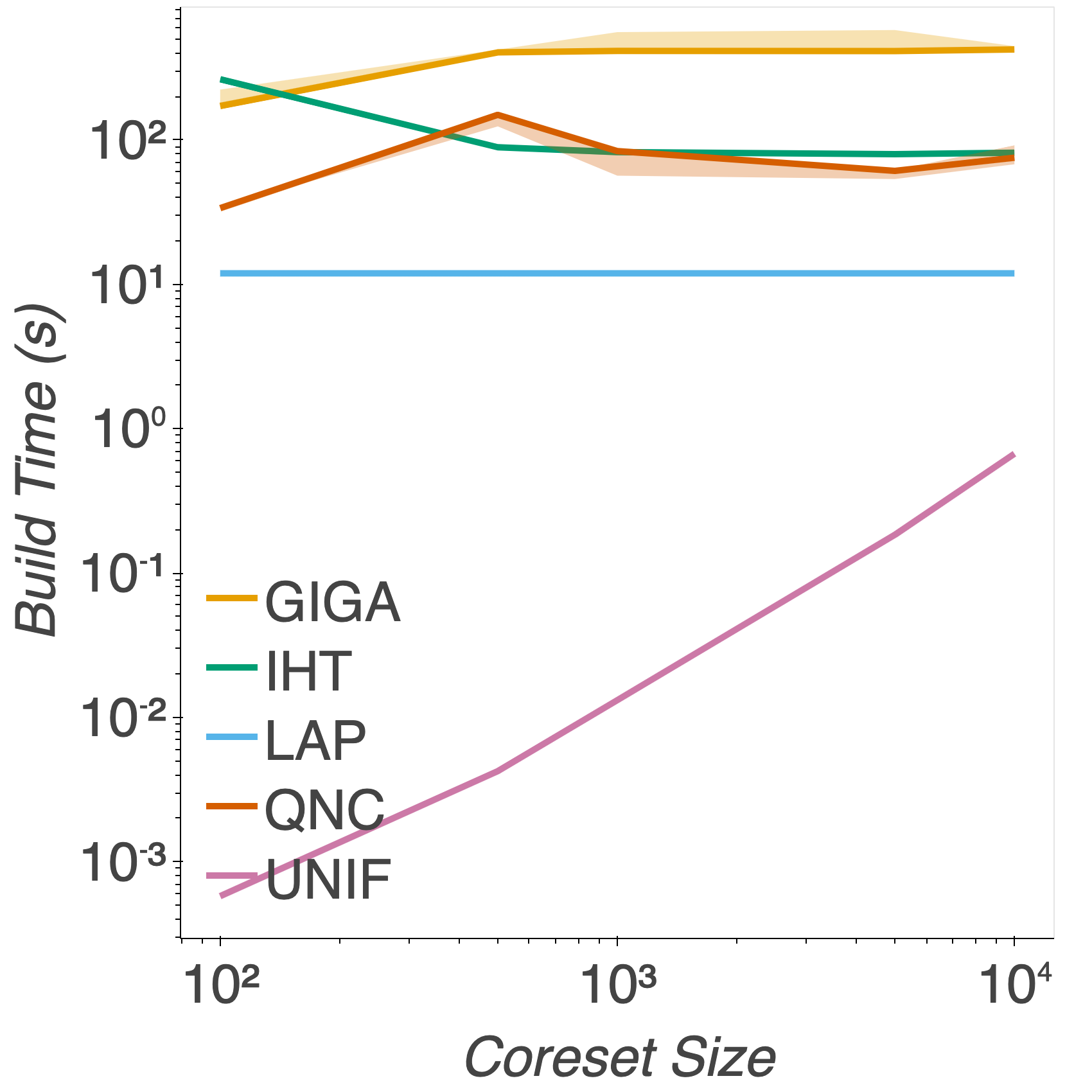
(a) Gaussian

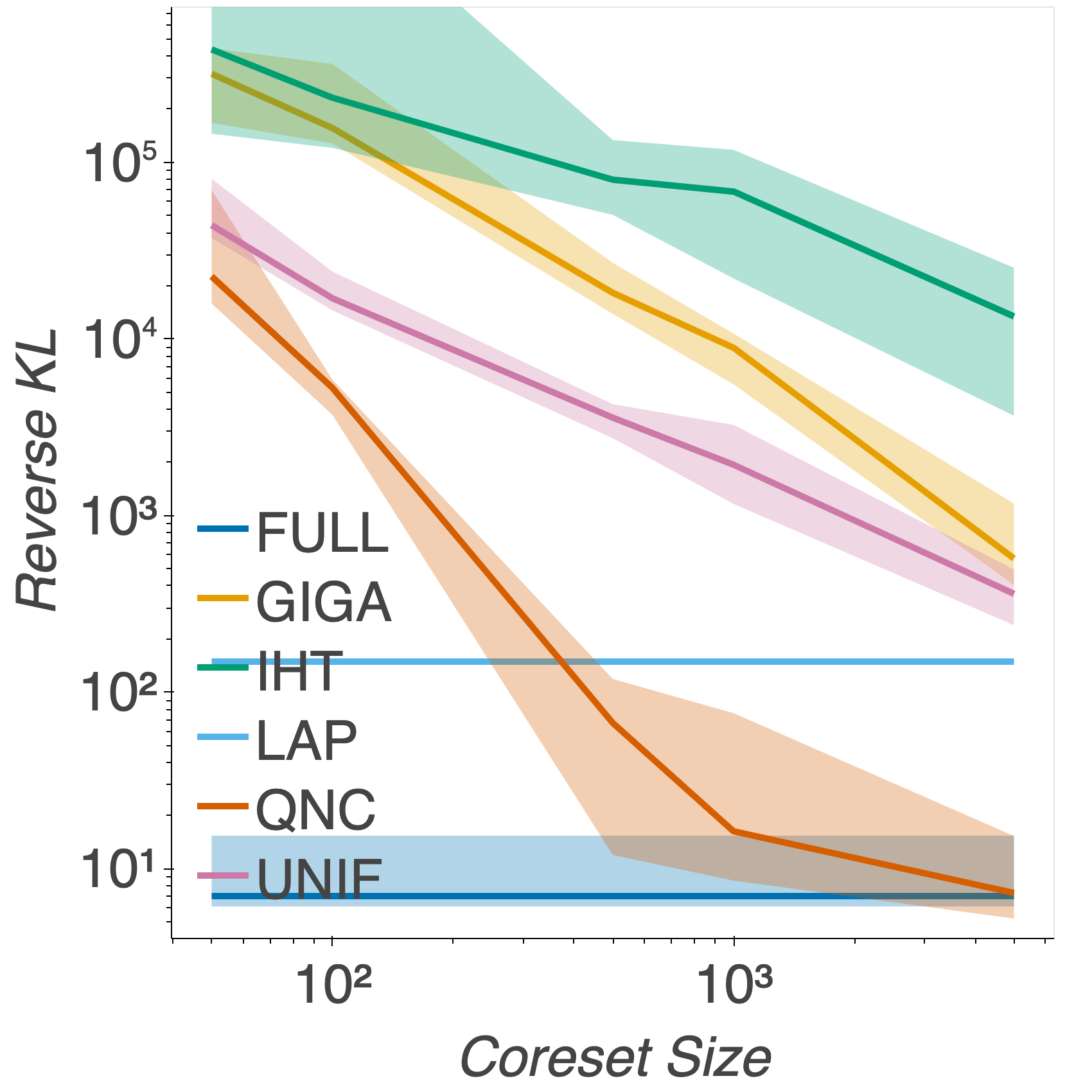
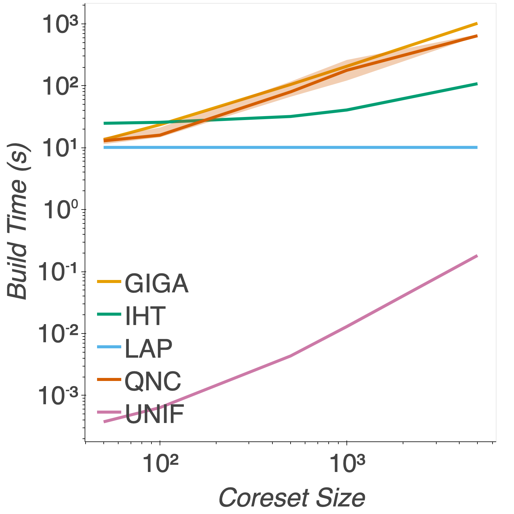
(b) Sparse linear regression

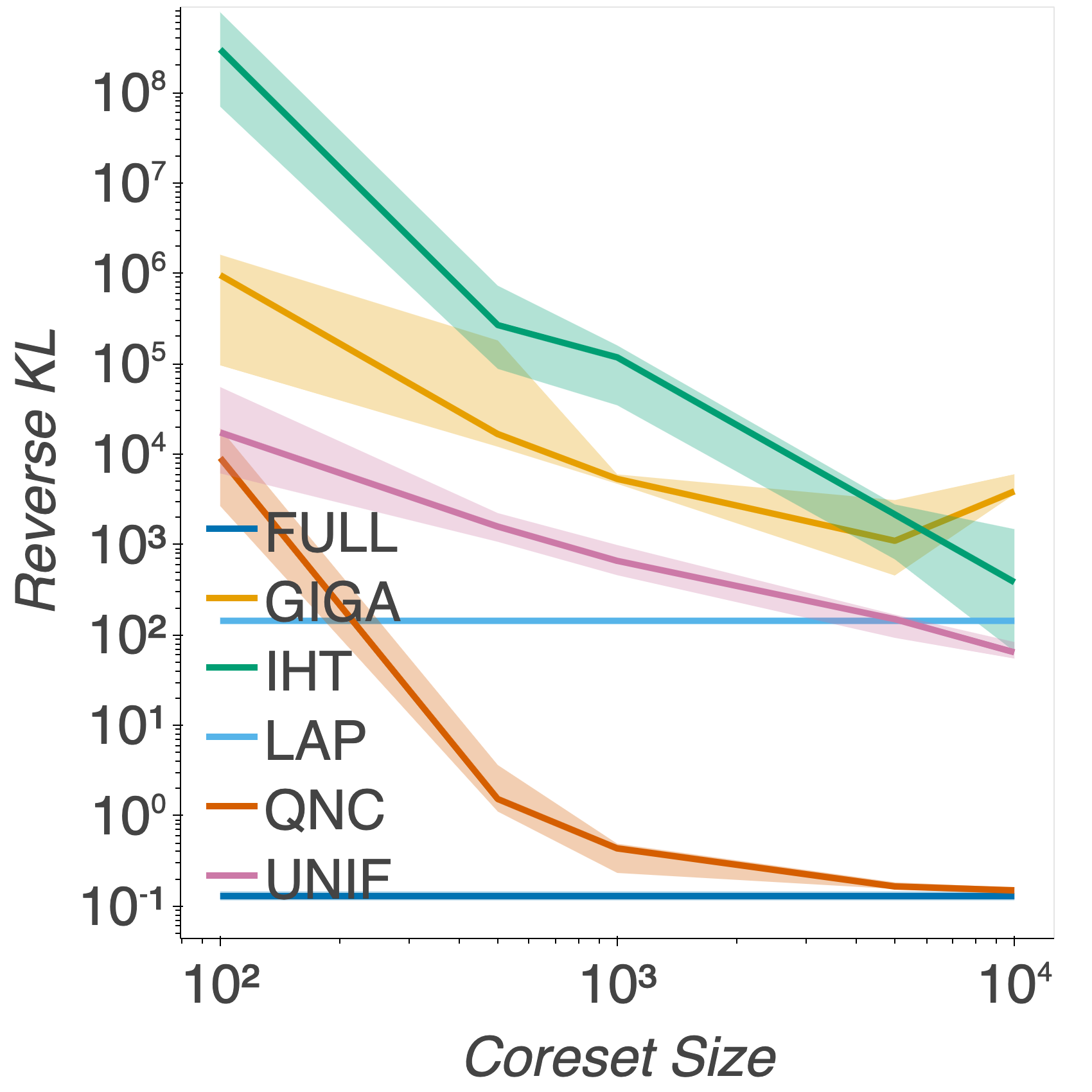
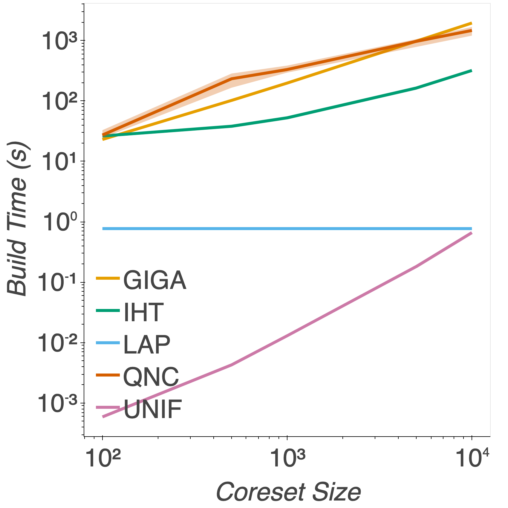
(c) Logistic regression

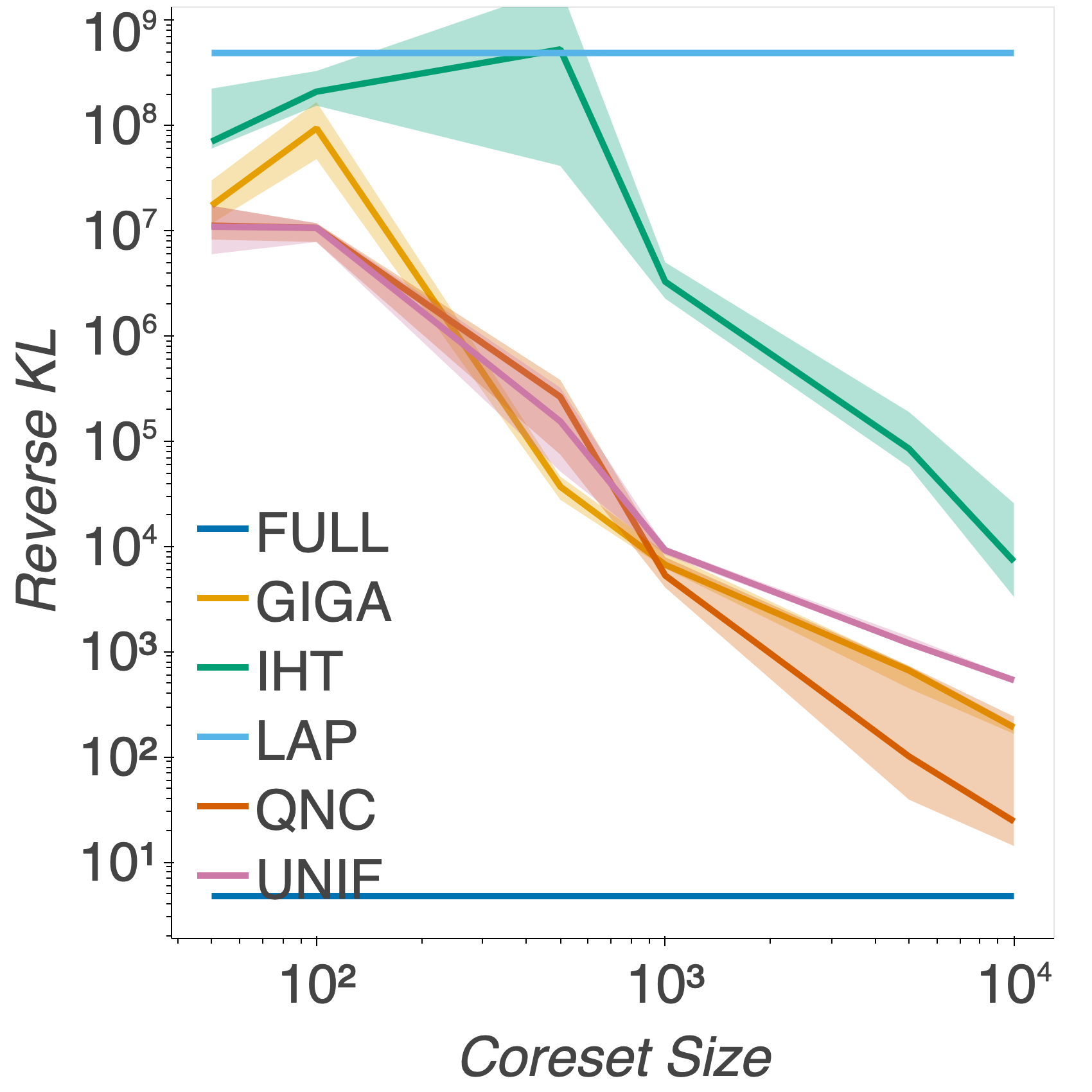
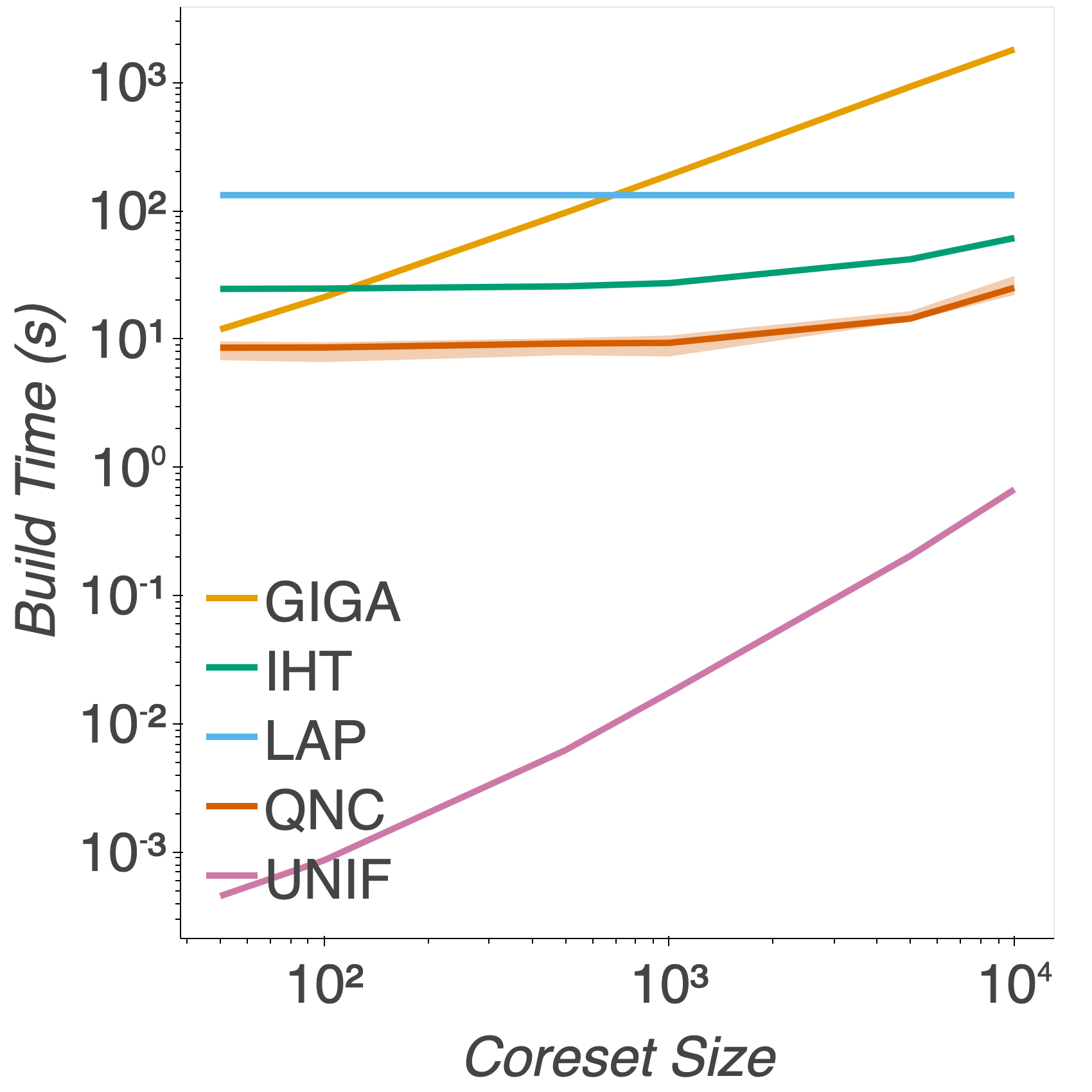
(d) Basis function regression

Figure 1: Reverse KL divergence (left) and build time in seconds (right) for each experiment. We plot the median and a shaded area between the 25${}^{\text{th}}$/75${}^{\text{th}}$ percentiles over 10 random trials. Our algorithm (QNC) provides an improvement in coreset quality, with a comparable run-time and less user input.

5.1 Synthetic Gaussian location model

Our first comparison is on a Gaussian location model, with prior $\theta\sim\mathcal{N}(\mu_{0},\sigma_{0}I)$, and likelihood $(X_{n})_{n=1}^{N}\overset{\text{i.i.d.}}{\sim}\mathcal{N}(\theta,\sigma I)$ in $D$ dimensions. Here, we take $\mu_{0}=0$ and $\sigma_{0}=1$. Closed form expressions are available for the subsampled posterior distributions [21, Appendix B], and we can sample from them without MCMC. We compare the methods on a synthetic dataset with $N=1,000,000$, $D=100$, where we generate the $(X_{n})_{n=1}^{N}\overset{\text{i.i.d.}}{\sim}\mathcal{N}(\mu,\sigma I)$ and set $(\mu_{i})_{i=1}^{D}\overset{\text{i.i.d.}}{\sim}\mathcal{N}(0,100)$ and $\sigma=100$. From Fig. 9(a) we see that our method outperforms the other subsampling methods for all coreset sizes. This example is largely illustrative; we expect LAP to provide the exact posterior here by design, and this is indeed what we find (the reverse KL plots for LAP and FULL overlap).

5.2 Bayesian sparse linear regression

Next, we study a Bayesian sparse linear regression problem, where the data $\left(x_{n},y_{n}\right)_{n=1}^{N}$ consists of a feature $x_{n}\in\mathbb{R}^{D}$ and an outcome $y_{n}\in\mathbb{R}^{N}$. The posterior distribution is that of $\theta\in\mathbb{R}^{D}$ in the model

$$y_{n}=x_{n}^{T}\theta+\epsilon_{n},\quad n=1,\ldots,N$$ (16)

where $\epsilon_{n}\overset{\text{i.i.d.}}{\sim}\mathcal{N}(0,\sigma),\ n=1,\ldots,N$. We place independent Cauchy priors on the coefficients $\theta$:

$$\theta_{i}\overset{\text{i.i.d.}}{\sim}\text{Cauchy}(0,\tau\lambda_{i}),\quad i=1,\ldots,D,$$

where the hyperpriors are $\lambda_{i}\overset{\text{i.i.d.}}{\sim}\text{Half-Cauchy}(0,1)$, $\tau\sim\text{Half-Cauchy}(0,\sigma_{0})$, with $\sigma_{0}=2$, and $\sigma\sim\Gamma(a_{0},b_{0})$ with $a_{0}=1,b_{0}=1$. We perform posterior inference on the $2D+2-$dimensional set of parameters $(\theta_{1},\ldots,\theta_{D},\lambda_{1},\ldots,\lambda_{D},\sigma,\tau)$. Sampling is performed using STAN [31]. The dataset we study is a flight delays dataset, with $N=100,000$ and $D=13$ (so that the overall inference problem is $28-$dimensional). The response variable $y_{n}$ is the delay in the departure time of a flight, and the features are meteorological and flight-specific information. We see in Fig. 9(c) that our method outperforms the other subsampling methods for all coreset sizes, and LAP for sizes above $500$—representing $0.5\%$ of the data. In Appendix C we see that the target posterior in this case has heavy tails, which makes the Laplace approximation particularly unsuited to this problem. We can see the effect this has even more clearly in the additional results presented there.

5.3 Heavy-tailed Bayesian logistic regression

For this comparison, we perform Bayesian logistic regression with parameter $\theta\in\mathbb{R}^{D}$ having a heavy-tailed Cauchy prior $\theta_{i}\overset{\text{i.i.d.}}{\sim}\text{Cauchy}(0,\sigma)$, $i=1,\dots,D$. The data $\left(x_{n},y_{n}\right)_{n=1}^{N}$ consists of a feature $x_{n}\in\mathbb{R}^{D}$ and a label $y_{n}\in\{-1,1\}$. The relevant posterior distribution is that of $\theta\in\mathbb{R}^{D}$ which governs the generation of $y_{n}$ given $x_{n}$ via

$$y_{n}\mid x_{n},\theta\stackrel{{\scriptstyle\text{ indep }}}{{\sim}}\operatorname{Bern}\left(\frac{1}{1+e^{-x_{n}^{T}\theta}}\right).$$ (17)

Again, sampling is performed using STAN. As in Section 5.2, we use the flight delays dataset, so we have that $N=100,000$ and $D=13$. The response variables $y_{n}$ are binarized, so that $y_{n}=1$ if a flight was cancelled or delayed by more than an hour, and $y_{n}=-1$ if it was not. In Fig. 1(c) we see that our method outperforms other subsampling methods for all coreset sizes, and LAP for sizes above $500$—representing $0.5\%$ of the data.

5.4 Bayesian radial basis function regression

Our final comparison is on a Bayesian basis function regression example. This is a larger version of the same experiment performed by [21], with $D=301$ as before, but $N=100,000$. Full details are given in Appendix C. From Fig. 1(d) we see that our method provides a significant improvement over LAP for all coreset sizes, which performs particularly poorly in this experiment, despite the Gaussianity of the target posterior [21, Appendix B]. It also outperforms the other subsampling methods for coreset sizes of 1000 and above (representing $1\%$ of the data) but this difference is not as marked as in the other examples. The fact that QNC requires a large coreset to start providing a benefit beyond UNIF stems from the fact that, in this higher dimensional example, there are sometimes data points that are very influential for a certain basis, and both UNIF and QNC can miss these. This indicates the need (in some settings) for a secondary method that can check for and include these, without the significant cost that e.g. SVI entails. We defer this study to future work. However, we do note that for this example QNC has the lowest build time, even outperforming LAP. This is because we only perform a small number of quasi-Newton steps before no further improvement is possible.

6 Conclusion

This paper introduces a novel method for data summarization prior to Bayesian inference. In particular, the method first selects a small subset of data uniformly randomly, and then optimizes the weights on those data points using a novel quasi-Newton method. Theoretical results demonstrate that the method is guaranteed to find a near-optimal coreset, and that the optimal coreset has a low KL divergence to the posterior with high probability. Future work includes investigating the performance of the method in more complex models, and studying conditions under which the method can provide compression in time sublinear in dataset size.

Checklist

1. For all authors…

   1. Do the main claims made in the abstract and introduction accurately reflect the paper’s contributions and scope? [Yes] The claims made in the abstract are supported by the theoretical and experimental results in Section 4 and Section 5

   2. Did you describe the limitations of your work? [Yes] Methodological limitations are discussed in Section 3.3 - mainly the fact that we need to used Monte Carlo estimates of some quantities of interest. The theoretical results in Section 4 show the setting in which our method can be expected to work. We give some intuition for what settings these are in the main text, with further discussion in Appendix A. In our fourth experiment in Section 5.4 we also discuss some of the limitations of our work in high dimensions.

   3. Did you discuss any potential negative societal impacts of your work? [No] Our work provides a generic preprocessing algorithm for sampling from probability distributions whose log density involves many summed terms. Our method is generic and foundational in nature: it has many downstream applications, including Bayesian inference, which may have a societal impact depending on the particular data and model under consideration. But we do not speculate on the impacts of potential downstream applications in this work.

   4. Have you read the ethics review guidelines and ensured that your paper conforms to them? [Yes]

2. If you are including theoretical results…

   1. Did you state the full set of assumptions of all theoretical results? [Yes] The assumptions for Theorem 4.1 and Theorem 4.3 are given in the theorem statements. Before the statement of Theorem 4.2 we give intuitive explanations of its assumptions, but the full assumptions are explicitly laid out in Appendix A.

   2. Did you include complete proofs of all theoretical results? [Yes] Proofs of all theoretical results are included in Appendix B.

3. If you ran experiments…

   1. Did you include the code, data, and instructions needed to reproduce the main experimental results (either in the supplemental material or as a URL)? [Yes] Code, data, and instructions needed to reproduce all experimental results is provided in the supplemental material.

   2. Did you specify all the training details (e.g., data splits, hyperparameters, how they were chosen)? [Yes] Important details are provided in Section 5, and all further details are included in the code provided as part of the supplemental material.

   3. Did you report error bars (e.g., with respect to the random seed after running experiments multiple times)? [Yes] Error bars representing the 25${}^{\text{th}}$/75${}^{\text{th}}$ percentiles over 10 random trials are presented for each plot of the results.

   4. Did you include the total amount of compute and the type of resources used (e.g., type of GPUs, internal cluster, or cloud provider)? [Yes] The details of the machine used to perform all experiments are given in Section 5.

4. If you are using existing assets (e.g., code, data, models) or curating/releasing new assets…

   1. If your work uses existing assets, did you cite the creators? [Yes] Creators of all existing assets are cited.

   2. Did you mention the license of the assets? [Yes] All the datasets we use are publicly available, and some do not include a license. Where relevant, the license is mentioned.

   3. Did you include any new assets either in the supplemental material or as a URL? [Yes] We include new code in the supplemental material.

   4. Did you discuss whether and how consent was obtained from people whose data you’re using/curating? [No] The datasets we use are publicly available, and do not pertain to identifiable individuals. We obey the license terms of the data where applicable, but do not discuss whether consent was obtained from the data creators.

   5. Did you discuss whether the data you are using/curating contains personally identifiable information or offensive content? [No] None of the datasets we use contain personally identifiable information or offensive content.

5. If you used crowdsourcing or conducted research with human subjects…

   1. Did you include the full text of instructions given to participants and screenshots, if applicable? [N/A]

   2. Did you describe any potential participant risks, with links to Institutional Review Board (IRB) approvals, if applicable? [N/A]

   3. Did you include the estimated hourly wage paid to participants and the total amount spent on participant compensation? [N/A]

Appendix A Theoretical analysis

In this section we give further details on the theoretical results presented in Section 4. We start by giving the exact conditions needed for Theorem 4.2 to hold.

A.1 Full conditions for Theorem 4.2

In order to state Theorem 4.2, we define $\theta_{0}$ as the unique value such that $\bar{f}(\theta)\leq\bar{f}(\theta_{0})$ $\forall\theta\in\Theta$, where $\bar{f}(\cdot)=\mathbb{E}_{p}(f_{n}(\cdot))$. If we split $f(x;\theta)$ into two parts,

$$f(x,\theta)=f^{(1)}(x,\theta)+f^{(2)}(x,\theta),$$

then we require that there exist constants $\epsilon_{0},L_{0},L_{1},L_{2}>0$ such that:

$\bullet$ A1: For all $x$, $f(x,\theta)$ is differentiable and strongly concave in $\theta$ with constant $L_{0}$.
$\bullet$ A2: For all $0<\epsilon<\epsilon_{0}$ and $\|\theta-\theta_{0}\|\leq\epsilon$,

$$|f^{(2)}(x,\theta)|\leq R(x)r(\epsilon)\|\theta-\theta_{0}\|^{2},$$

where $R(x),r(\epsilon)$ are positive functions, $r$ is monotone increasing, $\lim_{\epsilon\to 0}r(\epsilon)=0$, and

$$4r(\epsilon_{0})\left[\mathbb{E}_{p}(R(X))+1\right]\leq L_{0},\quad\mathbb{E}_{p}(R(X)^{2})<\infty.$$

$\bullet$ A3: For all $\|\theta-\theta_{0}\|\leq\epsilon_{0}$,

$$\bar{f}(\theta_{0})-\bar{f}(\theta)\leq L_{1}\|\theta-\theta_{0}\|^{2},\quad\mathrm{Var}_{p}(f(X;\theta_{0})-f(X;\theta))\leq L_{2}\|\theta-\theta_{0}\|^{2}.$$

$\bullet$ A4: $\inf_{\|\theta-\theta_{0}\|\leq\epsilon_{0}}\pi_{0}(\theta)>0$, and $\sup_{\theta}\pi_{0}(\theta)<\infty$.

Here, the functions $R(x),r(\epsilon)$ control the size of the “discarded part” $f^{(2)}$ locally around $\theta_{0}$; these should be small to ensure that $f(x,\theta)\approx f^{(1)}(x,\theta)$ locally. Note also that when $r(\epsilon)\asymp\epsilon$ as $\epsilon\to 0$, the result of Theorem 4.2 holds even if $D$ is increasing such that $D=o(\log N)$.

A.2 Discussion on conditions of Theorems 4.1, 4.2 and 4.3

In order for Theorem 4.1 to hold, we require that $S_{0}$ is finite dimensional (say with dimension $d$), where $S_{0}$ is the vector space of functions on $\Theta$ spanned by $\{f(x,\cdot);x\in\mathcal{X}\}$. For this to hold, we need to find a set of $d$ basis functions for the space, even though $\mathcal{X}$ may be potentially uncountable. There are two settings in which we can clearly see that this holds. The first of these is when $f(x_{n},\theta)=\log p(x_{n}|\theta)$ and we can write the likelihood as a $d$-dimensional exponential family. The standard exponential family form gives us the desired basis for $S_{0}$. The second setting is when $\mathcal{X}$ is in fact a finite set. If $x\in\mathcal{X}$ can only take $d$ values, then we can easily find a basis as before.

In the exponential family case, we can gain some more intuition on the behaviour of $J(\delta)$. Consider a full rank, $d$-dimensional exponential family with $f_{n}(\theta)=\log p(x_{n}|\theta)$. We can write

$$(f_{1}-\bar{f})(\theta)=A(\theta)^{T}(B(X_{1})-\mathbb{E}_{p}(B(X_{1})))-K(X_{1}),$$

where $X_{1}$ is the first observed data point (corresponding to the potential $f_{1}$), $B(\cdot)$ is the (full rank) sufficient statistic and $A(\theta)$ is the natural parameter. $K(X_{1})$ arises from the log-base density, and is a function of $X$ only. If there exists $\mu$ such that $R_{A}\coloneqq\int A(\theta)A(\theta)^{T}d\mu(\theta)$ has rank $d$, then

$$J(\delta)\xrightarrow{\delta N\to\infty}\inf_{a\in S_{0};\|a\|=1}\Pr\left(\langle a,f_{1}-\bar{f}\rangle_{L^{2}(\mu)}>0\right)>0.$$

We can see this as follows. Firstly, $J(\delta)$ is monotonically increasing as $\delta N\to\infty$. Hence, we can interchange the limit with the infimum to see that

$$\lim_{\delta N\to\infty}J(\delta)=\inf_{a\in S_{0};\|a\|=1}\Pr\left(\langle a,f_{1}-\bar{f}\rangle_{L^{2}(\mu)}>\lim_{\delta N\to\infty}\frac{2r_{\mu}}{\sqrt{N\delta}}\right),$$

and $\lim_{\delta N\to\infty}\frac{2r_{\mu}}{\sqrt{N\delta}}=0$. To see that this limit is strictly positive, note that the rank condition means that $S_{0}=\text{span}\left(A_{1}(\theta),\ldots,A_{d}(\theta)\right)$. Thus, $a\in S_{0}\iff a=V^{T}A$ for some $V$. Choosing $\mu$ such that $\mathbb{E}_{\mu}(A)=0$,

$$\langle a,f_{1}-\bar{f}\rangle_{L^{2}(\mu)} =V^{T}\left(\int A(\theta)A(\theta)^{T}d\mu(\theta)\right)(B(X_{1})-\mathbb{E}_{p}(B(X_{1})))-V^{T}\mathbb{E}_{\mu}(A)K(X_{1})$$

$$=V^{T}R_{A}(B(X_{1})-\mathbb{E}_{p}(B(X_{1})))\qquad\text{using our choice of $\mu$}.$$

Thus

$$\Pr\left(\langle a,f_{1}-\bar{f}\rangle_{L^{2}(\mu)}\geq 0\right)=\Pr\left(V^{T}R_{A}(B(X_{1})-\mathbb{E}_{p}(B(X_{1})))\geq 0\right).$$

Furthermore, $\|a\|=1\iff V^{T}R_{A}V=1$. Since $\mathbb{E}_{p}\left(V^{T}R_{A}(B(X_{1})-\mathbb{E}_{p}(B(X_{1})))\right)=0$,

$$\Pr\left(V^{T}R_{A}(B(X_{1})-\mathbb{E}_{p}(B(X_{1})))\geq 0\right)=0$$

$$\iff V^{T}R_{A}(B(X_{1})-\mathbb{E}_{p}(B(X_{1})))=0\quad\text{almost surely}.$$

However, this is impossible since both $R_{A}$ and $B$ are of full rank. Thus, $\forall V$, $\Pr(V)\coloneqq\Pr\left(V^{T}R_{A}(B(X_{1})-\mathbb{E}_{p}(B(X_{1})))\geq 0\right)>0$. Now, if $\exists V_{n}$ such that $\Pr(V_{n})\to 0$, the fact that we are on the compact space $\|a\|=1$ means that there exists a subsequence $V_{n_{k}}\to V_{*}$ with $V_{*}^{T}R_{A}V_{*}=1$. We would then have

$$V_{n_{k}}^{T}R_{A}(B(X_{1})-\mathbb{E}_{p}(B(X_{1})))\xrightarrow{d}V_{*}^{T}R_{A}(B(X_{1})-\mathbb{E}_{p}(B(X_{1}))),$$

where $\xrightarrow{d}$ indicates convergence in distribution. Then at the limit, $\Pr(V_{*})=0$, which we have shown is impossible. Thus, we do indeed have that

$$\lim_{\delta N\to\infty}J(\delta)=\inf\Pr(V)>0.$$

In this case, we can set $\delta=\omega(1/N)$, such that with probability $\geq 1-\omega(1/N)$, we indeed have that $\min_{w\in\mathcal{W}_{N}}\mathrm{KL}(\pi_{w}||\pi)=0$ for $M\gtrsim d\log N$.

In order for Theorem 4.2 to hold, we require additional smoothness and concavity conditions on $f(x,\theta)$. The smoothness conditions are satisfied if, for example, $f(x;\theta)$ is $C^{3}$ in $\theta$, as discussed in Section 4. For example, we can consider a logistic regression problem. Here, we are not in the exponential family setting. However, the logistic regression log-likelihood is concave and $C^{3}$ in $\theta$. Hence we can find $f^{(1)}$ and $f^{(2)}$ via a second-order Taylor expansion. Finally, A4 is satisfied by any prior that is strictly positive and finite, such as the Cauchy prior we use in our logistic regression experiment.

However, the logistic log-likelihood is concave but not strictly concave. Thus A1 does not hold, and our logistic regression experiment is not covered by the assumptions of Theorem 4.2. It is therefore reassuring to see that our method obtains favourable empirical results in this experiment, and we conjecture that the strong concavity condition is sufficient but not necessary. We leave the relaxing of this condition to future work.

In the statement of Theorem 4.3, we suppose that $\exists$ $\epsilon\in[0,1)$ and $\delta\geq 0$ such that for all $w\in W$

$$\|\left(G(w)\!+\!\tau I\right)^{-1}H(w)(1\!-\!w^{\star})\|\leq\epsilon\|w\!-\!w^{\star}\|\!+\!\delta,$$ (18)

where $w^{\star}=\mathrm{proj}_{W^{\star}}(w)$ and $W^{\star}\subseteq\arg\!\min_{w\in W}\mathrm{KL}(\pi_{w}||\pi)$.

If we can show that

$$\forall\theta\in\Theta,\quad\sum_{m=1}^{M}w^{\star}_{m}f_{m}(\theta) =\sum_{n}f_{n}(\theta),$$ (19)

then

$$H(w)(1-w^{\star}) =\mathrm{Cov}_{w}\left[g,f^{T}(1-w^{\star})\right]$$

$$=0.$$ (20)

and so thus the assumption will hold with $\epsilon=\delta=0$.

Theorem 4.1 tells us that $\pi_{w^{\star}}(\theta)=\pi(\theta)$ for almost all values of $\theta$. This implies that Eq. 19 also holds for almost all values of $\theta$, and so Eq. 20 holds. This means that the assumption in Theorem 4.3 does in fact hold with $\epsilon=\delta=0$.

Thus, in any setting where the conditions of Theorem 4.1 hold (such as the two discussed above), Theorem 4.3 holds as well. This reasoning also gives us some intuition into how we can generalise this. Intuitively, we require that

$$\forall\theta\in\Theta,\quad\sum_{m=1}^{M}w^{\star}_{m}f_{m}(\theta) \approx\sum_{n}f_{n}(\theta),$$ (21)

so that $H(w)(1-w^{\star})\approx 0$. Essentially, we see that the better the quality of the optimal coreset $w^{\star}$, the tighter the bound we can find for Eq. 18. We conjecture that if $\exists\ \xi$ such that we can uniformly bound

$$\sup_{\theta\in\Theta}\left|\sum_{m=1}^{M}w^{\star}_{m}f_{m}(\theta)-\sum_{n}f_{n}(\theta)\right|\leq\xi,$$

then we can find $\epsilon$ and $\delta$ such that Eq. 18 holds. We leave the theoretical examination of this claim for future work.

Appendix B Proofs

In this section we give the full proofs of Theorems 4.1, 4.2 and 4.3. The proofs of Theorems 4.1 and 4.2 are quite technical, so in each case we give start by giving a roadmap of the proof ideas.

B.1 Proof of Theorem 4.1

Roadmap.

1. We start the proof by giving in Eq. 22 a sufficient condition for our desired result to hold. Proving that this condition holds will be the target of the rest of the proof.

2. The next step is to show that this is indeed a sufficient condition. We do this by deriving the form for the KL divergence found in Eq. 25.

3. We then proceed by lower bounding the probability that the quantity on the right side of Eq. 22 lies within a ball of a given radius.

4. Next, we find a lower bound for the probability that we can get the left hand side of Eq. 22 to be equal to any value within the same ball as above.

5. If the events introduced in 2. and 3. hold, then we will be able to satisfy our sufficient condition Eq. 22. This implies that our desired result will also hold. Thus we can combine the two relevant lower bounds detailed in 2. and 3. to get a lower bound on the probability of our desired result holding.

6. Obtaining this final lower bound requires setting a condition on the coreset size $M$. We conclude the proof by rewriting condition to make it more interpretable.

Proof.

We select $M$ indices uniformly at random from $[N]$, corresponding to $M$ potential functions $f_{n}(\theta)$. Because the functions $f_{n}$ are generated i.i.d. and the indices chosen uniformly, the particular indices selected are unimportant for this proof; without loss of generality, we can assume the $M$ selected indices are $n=1,\dots,M$.

Let $\mu$ be a probability measure such that $S_{0}$ is the associated $d$ dimensional subspace of $L^{2}(\mu)$ and let $M\in[N]$. In what follows, we assume that all norms and inner products are the weighted $L^{2}(\mu)$ norms and inner products respectively, unless otherwise stated. Further, define $\widetilde{f}_{N}(\cdot)=\sum_{n=1}^{N}[f_{n}-\bar{f}](\cdot)/N$. We show below that with probability $\geq 1-\delta$, there exists $v_{1},\cdots,v_{M}\geq 0$ with $\sum_{m}v_{m}=1$ such that

$$\sum_{m=1}^{M}(f_{m}-\bar{f})v_{m}=\widetilde{f}_{N}.$$ (22)

For such a $v=(v_{1},\cdots,v_{M})$, set $w(v)=Nv$ (with the implicit convention that $w(v)_{j}=0$ for $j>M$). Our goal is to prove that $\mathrm{KL}(\pi_{w(v)}||\pi)=0$. We do this by starting with the form for the KL divergence derived in the proof of Lemma 3 of Campbell and Beronov [21]:

$$\mathrm{KL}(\pi_{w(v)}||\pi)=2(1-w)^{T}\mathbb{E}\left[C(\gamma(T))\right](1-w),$$

where:

• $T\sim\text{Beta}(1,2)$.

• $\gamma(t)$ is the path defined by $\gamma(t)=(1-t)w+t1$ for $t\in[0,1]$, coreset weights $w\in\mathbb{R}^{N}$, and unit vector $1\in\mathbb{R}^{N}$.

• $C(w)$ is the Fisher information metric Amari [32, p. 33,34] defined as:

  $$C(w) \coloneqq\operatorname{Cov}_{w}[f,f]$$

  $$\coloneqq\mathbb{E}_{\pi_{w}}\left[\left(f-\mathbb{E}_{\pi_{w}}(f)\right)\left(f-\mathbb{E}_{\pi_{w}}(f)\right)^{T}\right].$$

  Note that we have changed the notation from that of [21], to avoid a clash of notation with terms already defined in our work.

Using the fact that the p.d.f. of a $\text{Beta}(1,2)$ distribution is given by $f_{T}(t)=2(1-t)$, we therefore have that

$$\mathrm{KL}(\pi_{w(v)}||\pi) =2(1-w)^{T}\mathbb{E}\left[C(\gamma(T))\right](1-w)$$

$$=2(1-w)^{T}\left[\int_{0}^{1}2(1-t)C(\gamma(t))\mathrm{d}t\right](1-w)$$

$$=4(1-w)^{T}\left[\int_{0}^{1}(1-t)\mathbb{E}_{w(v),t}\left[\left(f-\mathbb{E}_{\pi_{\gamma(t)}}(f)\right)\left(f-\mathbb{E}_{\pi_{\gamma(t)}}(f)\right)^{T}\right]\mathrm{d}t\right](1-w)$$

$$=4\int_{0}^{1}(1-t)\mathbb{E}_{w(v),t}\left[\left((1-w)^{T}\left(f-\mathbb{E}_{w(v),t}(f)\right)\right)^{2}\right]\mathrm{d}t$$

$$=4\int_{0}^{1}(1-t)\mathbb{E}_{w(v),t}\left[\left(\sum_{n=1}^{N}(1-w_{n})f_{n}-\mathbb{E}_{w(v),t}\left(\sum_{n=1}^{N}(1-w_{n})f_{n}\right)\right)^{2}\right]\mathrm{d}t,$$ (23)

where $\mathbb{E}_{w(v),t}$ refers to taking expectations under $\pi_{w(v),t}$, the coreset posterior corresponding to weights given by $\gamma(t)=(1-t)w+t1$. To be explicit:

$$\pi_{w(v),t}(\theta)=\frac{e^{t\sum_{n}f_{n}+(1-t)\sum_{n}w_{n}f_{n}}\pi_{0}(\theta)}{\int_{\Theta}e^{t\sum_{n}f_{n}+(1-t)\sum_{n}w_{n}f_{n}}\pi_{0}(\theta)d\theta}.$$ (24)

We now note that

$$\frac{1}{N}\sum_{n=1}^{N}(1-w_{n})f_{n} =\frac{1}{N}\sum_{n=1}^{N}(f_{n}-\bar{f})-\frac{1}{N}\sum_{n=1}^{N}w_{n}(f_{n}-\bar{f})$$

$$=\widetilde{f}_{N}-\sum_{m}v_{m}(f_{m}-\bar{f}),$$

and thus

$$t\sum_{n}f_{n}+(1-t)\sum_{n}w_{n}f_{n} =\sum_{n}f_{n}-(1-t)\sum_{n}(1-w_{n})f_{n}$$

$$=\sum_{n}f_{n}-N(1-t)[\widetilde{f}_{N}-\sum_{m}v_{m}(f_{m}-\bar{f})].$$

Thus, by substituting into Eq. 24, we can write $\mathbb{E}_{w(v),t}$ as

$$\mathbb{E}_{w(v),t}(h)=\frac{\int_{\Theta}h(\theta)e^{\sum_{n}f_{n}(\theta)-N(1-t)[\widetilde{f}_{N}-\sum_{m}v_{m}(f_{m}-\bar{f})]}\pi_{0}(\theta)d\theta}{\int_{\Theta}e^{\sum_{n}f_{n}(\theta)-N(1-t)[\widetilde{f}_{N}-\sum_{m}v_{m}(f_{m}-\bar{f})]}\pi_{0}(\theta)d\theta}.$$

Furthermore, substituting into Eq. 23 we have that

$$\mathrm{KL}(\pi_{w(v)}||\pi) =4N^{2}\int_{0}^{1}(1-t)\mathbb{E}_{w(v),t}\left[\left(\widetilde{f}_{N}-\sum_{m}v_{m}(f_{m}-\bar{f})-\mathbb{E}_{w(v),t}\left(\widetilde{f}_{N}-\sum_{m}v_{m}(f_{m}-\bar{f})\right)\right)^{2}\right]\mathrm{d}t.$$ (25)

If we can prove Eq. 22, Eq. 25 would give us that $\mathrm{KL}(\pi_{w(v)}||\pi)=0$, thus completing the proof. Of course, if Eq. 22 holds then the coreset and full posteriors are equal, so $\mathrm{KL}(\pi_{w(v)}||\pi)$ is trivially zero. However, targeting this expression will also be helpful for the proof of Theorem 4.2. In order to prove Eq. 22, first note that $\|\widetilde{f}_{N}\|_{L^{2}(\mu)}^{2}=\mathbb{E}_{\mu}\left(\left(\frac{1}{N}\sum_{n}(f_{n}-\bar{f})\right)^{2}\right)$. With $r^{2}_{\mu}=\mathbb{E}_{\mu}\left(\mathbb{E}_{p}([f_{1}-\bar{f}]^{2})\right)$, we have by Markov’s inequality that, $\forall\delta>0$,

$$\Pr\left(\|\widetilde{f}_{N}\|_{L^{2}(\mu)}^{2}>\frac{r_{\mu}^{2}}{N\delta}\right) \leq\frac{N\delta}{r_{\mu}^{2}}\mathbb{E}_{p}\left(\mathbb{E}_{\mu}\left(\left(\frac{1}{N}\sum_{n}(f_{n}-\bar{f})\right)^{2}\right)\right)$$

$$=\frac{N\delta}{r_{\mu}^{2}}\mathbb{E}_{\mu}\left(\mathbb{E}_{p}\left(\left(\frac{1}{N}\sum_{n}(f_{n}-\bar{f})\right)^{2}\right)\right)$$

$$=\frac{N\delta}{r_{\mu}^{2}}\frac{1}{N}\mathbb{E}_{\mu}\left(\mathbb{E}_{p}\left(\left(f_{1}-\bar{f}\right)^{2}\right)\right)$$

$$=\delta.$$

Defining $t_{N}\coloneqq\sqrt{r_{\mu}^{2}/(N\delta)}$, it is enough to show that, with high probability, the convex hull of $(f_{m}-\bar{f}),m\in[M]$ contains the ball (in $S_{0}$) centered at 0 and with radius $t_{N}$. As in the theorem statement, $S_{0}$ is defined as the vector space of functions on $\Theta$ spanned by $\{f(x,\cdot);x\in\mathcal{X}\}$. This boils down to bounding

$$\Pr\left(\inf_{a\in S_{0};\|a\|=1}\max_{m}\langle a,f_{m}-\bar{f}\rangle\geq t_{N}\right)$$

from below, since on this event any point in the ball will be in the convex hull. Moreover, with probability $\geq 1-\delta$, $\widetilde{f}_{N}$ is in this ball, and thus Eq. 22 will be satisfied.

From Böröczky and Wintsche [33, Corollary 1.2], the unit sphere in $d$-dimensions can be covered by

$$N_{d}(\phi)=\frac{C\cdot\cos\phi}{\sin^{d}\phi}d^{\frac{3}{2}}\log(1+d\cos^{2}\phi)\leq\phi^{-d}A_{d},\quad A_{d}=Ce^{\frac{d}{2}}d^{\frac{3}{2}}\log(1+d)$$

balls of radius $0<\phi\leq\arccos\frac{1}{\sqrt{d+1}}$ and centers $(a_{i})_{i\leq N_{d}(\phi)}$, where $C$ is a universal constant. Moreover,

$$\inf_{a\in S_{0};\|a\|=1}\max_{m}\langle a,f_{m}-\bar{f}\rangle\geq\min_{i\leq N_{d}(\phi)}\max_{m=1,\dots,M}\left[\langle a_{i},f_{m}-\bar{f}\rangle-\phi\|f_{m}-\bar{f}\|_{L^{2}(\mu)}\right].$$

For any $a\in S_{0}$ with $\|a\|=1$, by independence,

$$\Pr \left(\max_{m=1,\dots,M}\left[\langle a,f_{m}-\bar{f}\rangle-\phi\|f_{m}-\bar{f}\|_{L^{2}(\mu)}\right]\leq t_{N}\right)$$

$$=\Pr\left(\langle a,f_{1}-\bar{f}\rangle-\phi\|f_{1}-\bar{f}\|_{L^{2}(\mu)}\leq t_{N}\right)^{M}.$$

For any $\phi>0$, if $\langle a,f_{1}-\bar{f}\rangle\leq 2t_{N}$ and $\|f_{1}-\bar{f}\|_{L^{2}(\mu)}>t_{N}/\phi$ then necessarily $\langle a,f_{1}-\bar{f}\rangle-\phi\|f_{1}-\bar{f}\|_{L^{2}(\mu)}\leq t_{N}$ by the triangle inequality. Thus, we can use the union bound to bound the above by

$$\Pr\left(\langle a,f_{1}-\bar{f}\rangle-\phi\|f_{1}-\bar{f}\|_{L^{2}(\mu)}\leq t_{N}\right)^{M}\leq\left[\Pr\left(\langle a,f_{1}-\bar{f}\rangle\leq 2t_{N}\right)+\Pr\left(\|f_{1}-\bar{f}\|>t_{N}/\phi\right)\right]^{M}$$

We have, for all $a\in S_{0}$ with $\|a\|=1$,

$$\Pr(\langle a,f_{1}-\bar{f}\rangle>2t_{N}) \geq\inf_{a\in S_{0};\|a\|=1}\Pr\left(\langle a,f_{1}-\bar{f}\rangle>2t_{N}\right)$$

$$=J(\delta),$$

using the definition of $J(\delta)$ as given in the statement of Theorem 4.1. Thus,

$$\Pr(\langle a,f_{1}-\bar{f}\rangle\leq 2t_{N})\leq 1-J(\delta).$$

Furthermore, choosing $\phi^{2}=J(\delta)/(4N\delta)$, we have by Chebychev’s inequality that

$$\Pr\left(\|f_{1}-\bar{f}\|>t_{N}/\phi\right)\leq J(\delta)/2.$$

Finally we obtain, using the union bound and the above results, that

$$\Pr\left(\inf_{a\in S_{0};\|a\|=1}\max_{m}\langle a,f_{m}-\bar{f}\rangle<t_{N}\right) \leq\Pr\left(\min_{i\leq N_{d}(\phi)}\max_{m=1,\dots,M}\left[\langle a_{i},f_{m}-\bar{f}\rangle-\phi\|f_{m}-\bar{f}\|_{L^{2}(\mu)}\right]<t_{N}\right)$$

$$\leq\sum_{i\leq N_{d}(\phi)}\Pr\left(\max_{m=1,\dots,M}\left[\langle a_{i},f_{m}-\bar{f}\rangle-\phi\|f_{m}-\bar{f}\|_{L^{2}(\mu)}\right]<t_{N}\right)$$

$$\leq\sum_{i\leq N_{d}(\phi)}\left[\Pr\left(\langle a_{i},f_{1}-\bar{f}\rangle\leq 2t_{N}\right)+\Pr\left(\|f_{1}-\bar{f}\|>t_{N}/\phi\right)\right]^{M}$$

$$\leq\sum_{i\leq N_{d}(\phi)}(1-J(\delta)+J(\delta)/2)^{M}$$

$$=N_{d}(\phi)(1-J(\delta)/2)^{M}.$$

For $M$ such that $MJ(\delta)\geq 4\log\left(N_{d}(\phi)\right)$, we then have that

$$N_{d}(\phi)(1-J(\delta)/2)^{M} \leq e^{MJ(\delta)/4}e^{M\log(1-J(\delta)/2)}$$

$$\leq e^{MJ(\delta)/4}e^{-MJ(\delta)/2}=e^{-MJ(\delta)/4}.$$

Using the union bound, we can therefore see that Eq. 22 holds with probability $\geq 1-\delta-e^{-MJ(\delta)/4}$.

Noting that $N_{d}(\phi)\leq\phi^{-d}A_{d}$, a sufficient condition on $M$ for this to hold is that

$$M \geq\frac{4}{J(\delta)}\log\left(\phi^{-d}A_{d}\right)$$

$$=\frac{4}{J(\delta)}\log\left(\left(\frac{J(\delta)}{4N\delta}\right)^{-d/2}A_{d}\right)$$

$$=\frac{2d}{J(\delta)}\left[\log N+\log\left(\frac{4\delta}{J(\delta)}\right)+\log\left(A_{d}^{2/d}\right)\right]$$

$$\geq\frac{2d}{J(\delta)}\left[\log N+\log\left(\frac{4\delta}{J(\delta)}\right)+C_{1}\right],$$

where $C_{1}$ is a constant such that $C_{1}\leq\log\left(A_{d}^{2/d}\right)$. This arrives at the condition on $M$ in the theorem statement, and thus completes the proof. ∎

B.2 Proof of Theorem 4.2

Roadmap.

1. The goal of this proof is to upper bound Eq. 25. We start by using a substitution to find an initial upper bound in the form of an integral.

2. Next, we split this integral up into two different terms, which we call $I_{\epsilon,1}$ and $I_{\epsilon,2}$, that together sum to the full integral as shown in Eq. 26. These terms can both be expressed as fractions, and share a common denominator. We will then find upper bound for these two terms separately.

3. We start by targeting $I_{\epsilon,1}$, and in particular upper bounding its numerator. We do this across a series of steps which provide sequential upper bounds. The aim is to find a final upper bound which is simpler, while retaining the necessary asymptotic properties. The final upper bound is given in Eq. 31.

4. As part of this process, we assume that a certain set of events occur, and lower bound the probability that they do. These probability bounds will be incorporated into the high probability bound for the final result.

5. Obtaining this upper bound on the numerator of $I_{\epsilon,1}$ also requires the introduction a condition similar to the one that was central to the proof of Theorem 4.1. This condition is given in Eq. 27.

6. Next, we lower bound the common denominator of $I_{\epsilon,1}$ and $I_{\epsilon,2}$. This involves a series of steps similar to those involved in upper bounding the numerator of $I_{\epsilon,1}$, and again we need to assume a set of events occurring. As before, we lower bound the probabilities that they do occur, and these probability bounds will be incorporated into the high probability bound for the final result. The final lower bound is given in Section B.2.

7. Similarly, we need to introduce two more important conditions that are required for our lower bound on the denominator to hold. These are given BY Eqs. 32 and 35.

8. So far, we have obtained in Section B.2 an upper bound on $I_{\epsilon,1}$, which holds with a probability that we have obtained a lower bound for, under certain specific conditions that we specify in LABEL:, 41, 42 and 43.

9. The next step is to upper bound $I_{\epsilon,2}$, and in particular its numerator (since we have already lower bounded its denominator). We do this using similar techniques to before, which introduces additional terms into the final high probability bounds. The final upper bound is given in Section B.2.

10. This gives us an upper bound on our original target (i.e. Eq. 25), which holds with a probability that we have lower bounded, and assuming that the conditions LABEL:, 41, 42 and 43 hold.

11. The final step is to lower bound the probability that LABEL:, 41, 42 and 43 all hold. This can be done in the same way as in the proof for Theorem 4.1, and we omit the full details.

12. Incorporating the above probability lower bounds, we finally have our desired upper bound for the original target, and a lower bound for the probability that this bound holds. This is what we refer to as our “high probability bound” in this roadmap.

Proof.

By the concavity and differentiability of $f(x,\cdot)$ we have $f(x;\theta)\leq f(x;\theta_{0})+\nabla_{\theta}f(x;\theta_{0})^{T}(\theta-\theta_{0})-L_{0}\|\theta-\theta_{0}\|^{2}$. Set $S_{N}(\theta_{0})=\sum_{n}\nabla_{\theta}f_{n}(\theta_{0})/\sqrt{N}$ and recall that by definition of $\theta_{0}$ as the maximizer of $\bar{f}=\mathbb{E}_{p}(f_{1}(\theta))$, $\mathbb{E}_{p}\left(\nabla_{\theta}f_{1}(\theta_{0})\right)=0$.

Starting from Eq. 25, we first use the fact that $\widetilde{f}_{N}(\cdot)=\sum_{n=1}^{N}[f_{n}-\bar{f}](\cdot)/N$ to rewrite

$$\widetilde{f}_{N}-\sum_{m}v_{m}(f_{m}-\bar{f})-\mathbb{E}_{w(v),t}[\widetilde{f}_{N}-\sum_{m}v_{m}(f_{m}-\bar{f})]$$

$$= \frac{\sum_{n}f_{n}(\theta)-f_{n}(\theta_{0})}{N}-\sum_{m}v_{m}(f_{m}(\theta)-f_{m}(\theta_{0}))-\mathbb{E}_{w(v),t}\left[\frac{\sum_{n}f_{n}(\theta)-f_{n}(\theta_{0})}{N}-\sum_{m}v_{m}(f_{m}(\theta)-f_{m}(\theta_{0}))\right].$$

Substituting this into Eq. 25, and using the fact that, for any random variable $X$, $\mathbb{E}\left[\left(X-\mathbb{E}(X)\right)^{2}\right]=\mathbb{E}\left(X^{2}\right)-\mathbb{E}\left(X\right)^{2}\leq\mathbb{E}\left(X^{2}\right)$, we can upper bound Eq. 25 by

$$\mathrm{KL}(\pi_{w(v)}||\pi)\leq 4N^{2}\int_{0}^{1}(1-t)\mathbb{E}_{w(v),t}\left[\left(\frac{1}{N}\sum_{n}f_{n}(\theta)-f_{n}(\theta_{0})-\sum_{m}v_{m}(f_{m}(\theta)-f_{m}(\theta_{0}))\right)^{2}\right]\mathrm{d}t.$$

We now decompose, for each $t\in(0,1)$, the integral over $\Theta$ in the above into an integral over $B_{\epsilon}=\{\|\theta-\theta_{0}\|\leq\epsilon\}$ and an integral over $B_{\epsilon}^{c}$. Here, $0<\epsilon<\epsilon_{0}$, where $\epsilon_{0}$ is as defined in the assumptions of Theorem 4.2. We can rewrite $\mathbb{E}_{w(v),t}(h)$ as

$$\mathbb{E}_{w(v),t}(h) =\frac{\int_{\Theta}h(\theta)e^{\sum_{n}f_{n}(\theta)-N(1-t)[\widetilde{f}_{N}(\theta)-\sum_{m}v_{m}(f_{m}(\theta)-\bar{f}(\theta))]}\pi_{0}(\theta)d\theta}{\int_{\Theta}e^{\sum_{n}f_{n}(\theta)-N(1-t)[\widetilde{f}_{N}(\theta)-\sum_{m}v_{m}(f_{m}(\theta)-\bar{f}(\theta))]}\pi_{0}(\theta)d\theta}$$

$$=\frac{\int_{\Theta}h(\theta)e^{t\sum_{n}f_{n}(\theta)+N(1-t)\sum_{m}v_{m}f_{m}(\theta)}\pi_{0}(\theta)d\theta}{\int_{\Theta}e^{t\sum_{n}f_{n}(\theta)+N(1-t)\sum_{m}v_{m}f_{m}(\theta)}\pi_{0}(\theta)d\theta}\times\frac{e^{-t\sum_{n}f_{n}(\theta_{0})-N(1-t)\sum_{m}v_{m}f_{m}(\theta_{0})}}{e^{-t\sum_{n}f_{n}(\theta_{0})-N(1-t)\sum_{m}v_{m}f_{m}(\theta_{0})}}$$

$$=\frac{\int_{\Theta}h(\theta)e^{t\sum_{n}(f_{n}(\theta)-f_{n}(\theta_{0}))+N(1-t)\sum_{m}v_{m}(f_{m}(\theta)-f_{m}(\theta_{0}))]}\pi_{0}(\theta)d\theta}{\int_{\Theta}e^{t\sum_{n}(f_{n}(\theta)-f_{n}(\theta_{0}))+N(1-t)\sum_{m}v_{m}(f_{m}(\theta)-f_{m}(\theta_{0}))]}\pi_{0}(\theta)d\theta}$$

$$=\frac{\int_{B_{\epsilon}^{c}}h(\theta)e^{t\sum_{n}(f_{n}(\theta)-f_{n}(\theta_{0}))+N(1-t)\sum_{m}v_{m}(f_{m}(\theta)-f_{m}(\theta_{0}))]}\pi_{0}(\theta)d\theta}{\int_{\Theta}e^{t\sum_{n}(f_{n}(\theta)-f_{n}(\theta_{0}))+N(1-t)\sum_{m}v_{m}(f_{m}(\theta)-f_{m}(\theta_{0}))]}\pi_{0}(\theta)d\theta}$$

$$\qquad+\frac{\int_{B_{\epsilon}}h(\theta)e^{t\sum_{n}(f_{n}(\theta)-f_{n}(\theta_{0}))+N(1-t)\sum_{m}v_{m}(f_{m}(\theta)-f_{m}(\theta_{0}))]}\pi_{0}(\theta)d\theta}{\int_{\Theta}e^{t\sum_{n}(f_{n}(\theta)-f_{n}(\theta_{0}))+N(1-t)\sum_{m}v_{m}(f_{m}(\theta)-f_{m}(\theta_{0}))]}\pi_{0}(\theta)d\theta}$$

$$\coloneqq I_{\epsilon,1}(h)+I_{\epsilon,2}(h)$$

Writing $I_{\epsilon,1}=I_{\epsilon,1}\left(\left(\frac{1}{N}\sum_{n}f_{n}(\theta)-f_{n}(\theta_{0})-\sum_{m}v_{m}(f_{m}(\theta)-f_{m}(\theta_{0}))\right)^{2}\right)$, and similarly for $I_{\epsilon,2}$, we can thus upper bound Eq. 25 by

$$KL(\pi_{w(v)}||\pi) \leq 4N^{2}\int_{0}^{1}(1-t)\left(I_{\epsilon,1}+I_{\epsilon,2}\right)\mathrm{d}t$$ (26)

We first prove that the integral $I_{\epsilon,1}$ over $B_{\epsilon}^{c}$ is small. Using the concavity bound for $f_{n}$, and recalling that $\sum_{m}v_{m}=1$, we have that

$$t\sum_{n}(f_{n}(\theta) -f_{n}(\theta_{0}))+N(1-t)\sum_{m}v_{m}(f_{m}(\theta)-f_{m}(\theta_{0}))$$

$$\leq t\sum_{n}\left(\nabla_{\theta}f_{n}(\theta_{0})^{T}(\theta-\theta_{0})-L_{0}\|\theta-\theta_{0}\|^{2}\right)+N(1-t)\sum_{m}v_{m}\left(\nabla_{\theta}f_{m}(\theta_{0})^{T}(\theta-\theta_{0})-L_{0}\|\theta-\theta_{0}\|^{2}\right)$$

$$=t\left[\sqrt{N}S_{N}(\theta_{0})^{T}(\theta-\theta_{0})-NL_{0}\|\theta-\theta_{0}\|^{2}\right]+N(1-t)\left[\sum_{m}v_{m}\nabla_{\theta}f_{m}(\theta_{0})^{T}(\theta-\theta_{0})-L_{0}\|\theta-\theta_{0}\|^{2}\right].$$

If

$$\sum_{m}v_{m}\nabla_{\theta}f_{m}(\theta_{0})=\frac{S_{N}(\theta_{0})}{\sqrt{N}}$$ (27)

then

$$t\sum_{n}(f_{n}(\theta)-f_{n}(\theta_{0})) +N(1-t)\sum_{m}v_{m}(f_{m}(\theta)-f_{m}(\theta_{0}))\leq\sqrt{N}S_{N}(\theta_{0})^{T}(\theta-\theta_{0})-NL_{0}\|\theta-\theta_{0}\|^{2}.$$

Using this bound, we can bound $I_{\epsilon,1}$ by

$$I_{\epsilon,1}$$

$$:=\frac{\int_{B_{\epsilon}^{c}}\left[\frac{1}{N}\sum_{n}f_{n}(\theta)-f_{n}(\theta_{0})-\sum_{m}v_{m}(f_{m}(\theta)-f_{m}(\theta_{0}))\right]^{2}e^{t\sum_{n}(f_{n}(\theta)-f_{n}(\theta_{0}))+N(1-t)\sum_{m}v_{m}(f_{m}(\theta)-f_{m}(\theta_{0}))]}\pi_{0}(\theta)d\theta}{\int_{\Theta}e^{t\sum_{n}(f_{n}(\theta)-f_{n}(\theta_{0}))+N(1-t)\sum_{m}v_{m}(f_{m}(\theta)-f_{m}(\theta_{0}))]}\pi_{0}(\theta)d\theta}$$

$$\leq\frac{\int_{B_{\epsilon}^{c}}\left[\frac{1}{N}\sum_{n}f_{n}(\theta)-f_{n}(\theta_{0})-\sum_{m}v_{m}(f_{m}(\theta)-f_{m}(\theta_{0}))\right]^{2}e^{\sqrt{N}S_{N}(\theta_{0})^{T}(\theta-\theta_{0})-NL_{0}\|\theta-\theta_{0}\|^{2}}\pi_{0}(\theta)d\theta}{\int_{\Theta}e^{t\sum_{n}(f_{n}(\theta)-f_{n}(\theta_{0}))+N(1-t)\sum_{m}v_{m}(f_{m}(\theta)-f_{m}(\theta_{0}))]}\pi_{0}(\theta)d\theta}.$$

Completing the square in the exponent of the numerator, we can rewrite it as

$$\sqrt{N}S_{N}(\theta_{0})^{T}(\theta-\theta_{0})-NL_{0}\|\theta-\theta_{0}\|^{2}$$

$$=-NL_{0}\left(\|\theta-\theta_{0}\|^{2}-\frac{S_{N}(\theta_{0})^{T}(\theta-\theta_{0})}{\sqrt{N}L_{0}}\right)$$

$$=-NL_{0}\left\|(\theta-\theta_{0})-\frac{S_{N}(\theta_{0})}{2\sqrt{N}L_{0}}\right\|^{2}+\frac{\|S_{N}(\theta_{0})\|^{2}}{4L_{0}}$$

We now assume that $\|S_{N}(\theta_{0})\|\leq\left(2-\sqrt{2}\right)\epsilon L_{0}\sqrt{N}$. By Markov’s inequality,

$$\Pr\left(\|S_{N}(\theta_{0})\|\geq\left(2-\sqrt{2}\right)\epsilon L_{0}\sqrt{N}\right) \leq\frac{\mathbb{E}_{p}\left(\|S_{N}(\theta_{0})\|^{2}\right)}{\left(2-\sqrt{2}\right)^{2}\epsilon^{2}NL_{0}^{2}}$$

$$\leq 3\frac{\mathbb{E}_{p}\left(\|\sum_{n}\nabla_{\theta}f_{n}(\theta_{0})\|^{2}\right)}{\epsilon^{2}N^{2}L_{0}^{2}}$$

$$=3\frac{\sum_{n}\mathbb{E}_{p}\left(\|\nabla_{\theta}f_{n}(\theta_{0})\|^{2}\right)}{\epsilon^{2}N^{2}L_{0}^{2}}$$

$$=3\frac{\mathbb{E}_{p}\left(\|\nabla_{\theta}f_{1}(\theta_{0})\|^{2}\right)}{\epsilon^{2}NL_{0}^{2}},$$

and thus the probability that $\|S_{N}(\theta_{0})\|\leq\left(2-\sqrt{2}\right)\epsilon L_{0}\sqrt{N}$ is bounded from below by $1-3\mathbb{E}_{p}(\|\nabla_{\theta}f_{1}(\theta_{0})\|^{2})/(L_{0}^{2}N\epsilon^{2})$. Here, and throughout, we assume that $N$ is large enough such that the relevant probabilities we use for our high-probability bounds are $\geq 0$. When this event occurs,

$$\left\|(\theta-\theta_{0})-\frac{S_{N}(\theta_{0})}{2\sqrt{N}L_{0}}\right\| \geq\left\|\theta-\theta_{0}\right\|-\left\|\frac{S_{N}(\theta_{0})}{2\sqrt{N}L_{0}}\right\|$$

$$\geq\left\|\theta-\theta_{0}\right\|-\frac{\left(2-\sqrt{2}\right)\epsilon L_{0}\sqrt{N}}{2\sqrt{N}L_{0}}$$

$$\geq\left\|\theta-\theta_{0}\right\|-\left(\frac{2-\sqrt{2}}{2}\right)\epsilon$$

$$\geq\left\|\theta-\theta_{0}\right\|-\left(\frac{2-\sqrt{2}}{2}\right)\left\|\theta-\theta_{0}\right\|\qquad\text{ on $B_{\epsilon}^{c}$}$$

$$=\frac{1}{\sqrt{2}}\|\theta-\theta_{0}\|.$$

Thus

$$\left\|(\theta-\theta_{0})-\frac{S_{N}(\theta_{0})}{2\sqrt{N}L_{0}}\right\|^{2}\geq\frac{1}{2}\|\theta-\theta_{0}\|^{2},$$

since both sides are positive numbers.

For ease of notation, we define $\Delta_{n}\coloneqq f_{n}(\theta)-f_{n}(\theta_{0})$. We can then bound $I_{\epsilon,1}$ by

$$I_{\epsilon,1} \leq\frac{e^{\frac{\|S_{N}(\theta_{0})\|^{2}}{4L_{0}}}\int_{B_{\epsilon}^{c}}\left[\frac{1}{N}\sum_{n}\Delta_{n}-\sum_{m}v_{m}\Delta_{m}\right]^{2}e^{-NL_{0}\left\|(\theta-\theta_{0})-\frac{S_{N}(\theta_{0})}{2\sqrt{N}L_{0}}\right\|^{2}}\pi_{0}(\theta)d\theta}{\int_{\Theta}e^{t\sum_{n}(f_{n}(\theta)-f_{n}(\theta_{0}))+N(1-t)\sum_{m}v_{m}(f_{m}(\theta)-f_{m}(\theta_{0}))]}\pi_{0}(\theta)d\theta}$$

$$\leq\frac{e^{\epsilon^{2}NL_{0}/8}\int_{B_{\epsilon}^{c}}\left[\frac{1}{N}\sum_{n}\Delta_{n}-\sum_{m}v_{m}\Delta_{m}\right]^{2}e^{-NL_{0}\|\theta-\theta_{0}\|^{2}/2}\pi_{0}(\theta)d\theta}{\int_{\Theta}e^{t\sum_{n}(f_{n}(\theta)-f_{n}(\theta_{0}))+N(1-t)\sum_{m}v_{m}(f_{m}(\theta)-f_{m}(\theta_{0}))]}\pi_{0}(\theta)d\theta}.$$

To further simplify the upper bound on the numerator, we define $\bar{\Delta}\coloneqq\mathbb{E}_{p}(\Delta_{n})$ and consider the event where

$$\int_{B_{\epsilon}^{c}}\left[\frac{1}{N}\sum_{n}\Delta_{n}-\sum_{m}v_{m}\Delta_{m}\right]^{2}e^{-NL_{0}\|\theta-\theta_{0}\|^{2}/2}\pi_{0}(\theta)d\theta\leq e^{-NL_{0}\epsilon^{2}/4}\int_{\Theta}\mathbb{E}_{p}(\Delta_{1}-\bar{\Delta})^{2}(\theta)\pi_{0}(\theta)d\theta.$$ (28)

The probability of Eq. 28 holding can be bounded from below by using Markov’s inequality,

$$\Pr \left(\int_{B_{\epsilon}^{c}}\left[\frac{1}{N}\sum_{n}\Delta_{n}-\sum_{m}v_{m}\Delta_{m}\right]^{2}e^{-NL_{0}\|\theta-\theta_{0}\|^{2}/2}\pi_{0}(\theta)d\theta>e^{-NL_{0}\epsilon^{2}/4}\int_{\Theta}\mathbb{E}_{p}(\Delta_{1}-\bar{\Delta})^{2}(\theta)\pi_{0}(\theta)d\theta\right)$$

$$\leq\frac{e^{NL_{0}\epsilon^{2}/4}\mathbb{E}_{p}\left(\int_{B_{\epsilon}^{c}}\left[\frac{1}{N}\sum_{n}\Delta_{n}-\sum_{m}v_{m}\Delta_{m}\right]^{2}e^{-NL_{0}\|\theta-\theta_{0}\|^{2}/2}\pi_{0}(\theta)d\theta\right)}{\int_{\Theta}\mathbb{E}_{p}(\Delta_{1}-\bar{\Delta})^{2}(\theta)\pi_{0}(\theta)d\theta}.$$ (29)

We now use the fact that $(a-b)^{2}\leq 2a^{2}+2b^{2}$ to bound

$$\left[\frac{1}{N}\sum_{n}\Delta_{n}-\sum_{m}v_{m}\Delta_{m}\right]^{2} =\left[\frac{\sum_{n}(\Delta_{n}-\bar{\Delta})}{N}-\sum_{m}v_{m}(\Delta_{m}-\bar{\Delta})\right]^{2}$$

$$\leq 2\left(\frac{\sum_{n}(\Delta_{n}-\bar{\Delta})}{N}\right)^{2}+2\left(\sum_{m}v_{m}(\Delta_{m}-\bar{\Delta})\right)^{2}$$

$$\leq 2\left(\frac{\sum_{n}(\Delta_{n}-\bar{\Delta})}{N}\right)^{2}+2\left(\max_{M}(\Delta_{m}-\bar{\Delta})\sum_{m}v_{m}\right)^{2}$$

$$\leq 2\left(\frac{\sum_{n}(\Delta_{n}-\bar{\Delta})}{N}\right)^{2}+2\max_{M}(\Delta_{m}-\bar{\Delta})^{2}.$$

Combined with the fact that $\|\theta-\theta_{0}\|\geq\epsilon$ on $B_{\epsilon}^{c}$, we can bound Eq. 29 above by

$$\leq\frac{2\left(\int_{B_{\epsilon}^{c}}\mathbb{E}_{p}\left[\left(\frac{\sum_{n}(\Delta_{n}-\bar{\Delta})}{N}\right)^{2}+\max_{M}(\Delta_{m}-\bar{\Delta})^{2}\right]e^{-NL_{0}\|\theta-\theta_{0}\|^{2}/4}\pi_{0}(\theta)d\theta\right)}{\int_{\Theta}\mathbb{E}_{p}(\Delta_{1}-\bar{\Delta})^{2}(\theta)\pi_{0}(\theta)d\theta}.$$ (30)

Then, by the definition of $\bar{\Delta}$, and the independence of the $f_{n}$ and therefore $\Delta_{n}$,

$$\mathbb{E}_{p}\left[\left(\frac{\sum_{n}(\Delta_{n}-\bar{\Delta})}{N}\right)^{2}+\max_{M}(\Delta_{m}-\bar{\Delta})^{2}\right] =\frac{1}{N^{2}}\sum_{n}\mathbb{E}_{p}\left((\Delta_{n}-\bar{\Delta})^{2}\right)+\mathbb{E}_{p}\left[\max_{M}(\Delta_{m}-\bar{\Delta})^{2}\right]$$

$$\leq\frac{1}{N}\mathbb{E}_{p}\left((\Delta_{1}-\bar{\Delta})^{2}\right)+\mathbb{E}_{p}\left[\sum_{m=1}^{M}(\Delta_{m}-\bar{\Delta})^{2}\right]$$

$$=\frac{1}{N}\mathbb{E}_{p}\left((\Delta_{1}-\bar{\Delta})^{2}\right)+M\mathbb{E}_{p}\left((\Delta_{1}-\bar{\Delta})^{2}\right).$$

Thus, Eq. 30 can be upper bounded by

$$\leq\frac{2\int_{B_{\epsilon}^{c}}e^{-NL_{0}\|\theta-\theta_{0}\|^{2}/4}\mathbb{E}_{p}(\Delta_{1}-\bar{\Delta})^{2}(\theta)\left(\frac{1}{N}+M\right)\pi_{0}(\theta)d\theta}{\int_{\Theta}\mathbb{E}_{p}(\Delta_{1}-\bar{\Delta})^{2}(\theta)\pi_{0}(\theta)d\theta}$$

$$\leq\frac{2\int_{B_{\epsilon}^{c}}e^{-NL_{0}\epsilon^{2}/4}\mathbb{E}_{p}(\Delta_{1}-\bar{\Delta})^{2}(\theta)\left(2M\right)\pi_{0}(\theta)d\theta}{\int_{\Theta}\mathbb{E}_{p}(\Delta_{1}-\bar{\Delta})^{2}(\theta)\pi_{0}(\theta)d\theta}$$

$$\leq 4Me^{-NL_{0}\epsilon^{2}/4}.$$

This tells us that the probability of Eq. 28 holding can be bounded from below by $1-4Me^{-NL_{0}\epsilon^{2}/4}$. We have now obtained an upper bound on the numerator of $I_{\epsilon,1}$ that holds with high probability. To summarize the result so far: if $\sum_{m}v_{m}\nabla_{\theta}f_{m}(\theta_{0})=\frac{S_{N}(\theta_{0})}{\sqrt{N}}$, we have that for any $0<\epsilon<\epsilon_{0}$,

$$I_{\epsilon,1}\leq\frac{e^{-\epsilon^{2}NL_{0}/8}\int_{\Theta}\mathbb{E}_{p}(\Delta_{1}-\bar{\Delta})^{2}(\theta)\pi_{0}(\theta)d\theta}{\int_{\Theta}e^{t\sum_{n}(f_{n}(\theta)-f_{n}(\theta_{0}))+N(1-t)\sum_{m}v_{m}(f_{m}(\theta)-f_{m}(\theta_{0}))}\pi_{0}(\theta)d\theta}.$$ (31)

with probability at least

$$1-4Me^{-NL_{0}\epsilon^{2}/4}-3\frac{\mathbb{E}_{p}\left(\|\nabla_{\theta}f_{1}(\theta_{0})\|^{2}\right)}{\epsilon^{2}NL_{0}^{2}}.$$

We continue by finding a lower bound for the denominator of $I_{\epsilon,1}$. We decompose $f_{n}$ into $f_{n}^{(1)}$ and $f_{n}^{(2)}$ and assume that

$$\sum_{m}v_{m}(f_{m}^{(1)}(\theta)-f_{m}^{(1)}(\theta_{0}))-\frac{\sum_{n}(f_{n}^{(1)}(\theta)-f_{n}^{(1)}(\theta_{0}))}{N}=0.$$ (32)

Then

$$t\sum_{n}(f_{n}(\theta)-f_{n}(\theta_{0}))+N(1-t)\left[\sum_{m}v_{m}(f_{m}(\theta)-f_{m}(\theta_{0}))\right]$$

$$=\sum_{n}(f_{n}(\theta)-f_{n}(\theta_{0}))+N(1-t)\left[\sum_{m}v_{m}(f_{m}(\theta)-f_{m}(\theta_{0}))-\frac{\sum_{n}(f_{n}(\theta)-f_{n}(\theta_{0}))}{N}\right]$$

$$=\sum_{n}(f_{n}(\theta)-f_{n}(\theta_{0}))+N(1-t)\left[\sum_{m}v_{m}(f_{m}^{(2)}(\theta)-f_{m}^{(2)}(\theta_{0}))-\frac{\sum_{n}(f_{n}^{(2)}(\theta)-f_{n}^{(2)}(\theta_{0}))}{N}\right]$$

$$=\sum_{n}(f_{n}(\theta)-f_{n}(\theta_{0}))+N(1-t)\left[\sum_{m}v_{m}f_{m}^{(2)}(\theta)-\frac{\sum_{n}f_{n}^{(2)}(\theta)}{N}\right],$$ (33)

using Eq. 32 and the fact that $f_{n}^{(2)}(\theta_{0})=0$ by assumption A2. For any $0<\epsilon^{\prime}<\epsilon_{0}$, and $\|\theta-\theta_{0}\|\leq\epsilon^{\prime}$, we use assumption A2 again, along with the fact that $a-b\geq-|a|-|b|$, to bound Eq. 33 from below by

$$\geq\sum_{n}(f_{n}(\theta)-f_{n}(\theta_{0}))-N(1-t)\left|\sum_{m}v_{m}f_{m}^{(2)}(\theta)-\frac{\sum_{n}f_{n}^{(2)}(\theta)}{N}\right|$$

$$\geq\sum_{n}(f_{n}(\theta)-f_{n}(\theta_{0}))-N(1-t)r(\epsilon^{\prime})\|\theta-\theta_{0}\|^{2}\left[\left|\sum_{m}v_{m}R(x_{m})\right|+\left|\frac{\sum_{n}R(x_{n})}{N}\right|\right]$$

$$\geq\sum_{n}(f_{n}(\theta)-f_{n}(\theta_{0}))$$

$$~{}~{}~{}~{}~{}~{}~{}~{}-N(1-t)r(\epsilon^{\prime})\|\theta-\theta_{0}\|^{2}\left[2\mathbb{E}_{p}(R(X))+\left|\sum_{m}v_{m}(R(x_{m})-\mathbb{E}_{p}(R(X)))\right|+\frac{\left|\sum_{n}(R(x_{n})-\mathbb{E}_{p}(R(X)))\right|}{N}\right]$$ (34)

using the fact that $R(x)>0$ by assumption. Next, we assume that

$$\left|\sum_{m}v_{m}(R(x_{m})-\mathbb{E}_{p}(R(X))\right|\leq 1\qquad\text{and}\qquad\frac{\left|\sum_{n}(R(x_{n})-\mathbb{E}_{p}(R(X))\right|}{N}\leq 1.$$ (35)

We can bound the probability of the second inequality holding from below by $1-\mathrm{Var}_{p}(R(X))/N$ via Chebychev’s inequality:

$$\Pr\left(\left|\frac{1}{N}\sum_{n}R(x_{n})-\mathbb{E}_{p}(R(X))\right|\geq\frac{\sqrt{\mathrm{Var}_{p}\left(\frac{1}{N}\sum_{n}R(x_{n})\right)}}{\sqrt{\mathrm{Var}_{p}\left(\frac{1}{N}\sum_{n}R(x_{n})\right)}}\right)\leq\mathrm{Var}_{p}\left(\frac{1}{N}\sum_{n}R(x_{n})\right)=\frac{1}{N}\mathrm{Var}_{p}(R(X)).$$

Substituting the two assumptions from Eq. 35 into Eq. 34 above, we obtain that

$$t\sum_{n}(f_{n}(\theta) -f_{n}(\theta_{0}))+N(1-t)\sum_{m}v_{m}(f_{m}(\theta)-f_{m}(\theta_{0}))$$

$$\geq\sum_{n}(f_{n}(\theta)-f_{n}(\theta_{0}))-2Nr(\epsilon^{\prime})\|\theta-\theta_{0}\|^{2}\left[\mathbb{E}_{p}(R(X))+1\right]$$

$$=\sum_{n}(f_{n}(\theta)-f_{n}(\theta_{0}))-\gamma Nr(\epsilon^{\prime})\|\theta-\theta_{0}\|^{2},\quad\text{where}\quad\gamma\coloneqq 2\left[\mathbb{E}_{p}(R(X))+1\right].$$

Then we can bound the denominator of $I_{\epsilon,1}$ from below by

$$\int_{\Theta}e^{t\sum_{n}(f_{n}(\theta)-f_{n}(\theta_{0}))+N(1-t)\sum_{m}v_{m}(f_{m}(\theta)-f_{m}(\theta_{0}))]}\pi_{0}(\theta)d\theta$$

$$\geq \int_{B_{\epsilon^{\prime}}}e^{t\sum_{n}(f_{n}(\theta)-f_{n}(\theta_{0}))+N(1-t)\sum_{m}v_{m}(f_{m}(\theta)-f_{m}(\theta_{0}))]}\pi_{0}(\theta)d\theta$$

$$\geq \int_{B_{\epsilon^{\prime}}}e^{\sum_{n}f_{n}(\theta)-f_{n}(\theta_{0})-\gamma Nr(\epsilon^{\prime})\|\theta-\theta_{0}\|^{2}}\pi_{0}(\theta)d\theta$$

$$\geq \pi_{0,\inf}\int_{B_{\epsilon^{\prime}}}e^{\sum_{n}f_{n}(\theta)-f_{n}(\theta_{0})-\gamma Nr(\epsilon^{\prime})\|\theta-\theta_{0}\|^{2}}d\theta$$

$$\geq \pi_{0,\inf}e^{-t_{a}(\epsilon^{\prime})}\int_{B_{\epsilon^{\prime}}}\mathrm{1}_{\sum_{n}f_{n}(\theta)-f_{n}(\theta_{0})\geq N(\bar{f}(\theta)-\bar{f}(\theta_{0}))-t_{a}}e^{-L_{1}^{\prime}(\epsilon^{\prime})N\|\theta-\theta_{0}\|^{2}}d\theta$$ (36)

$$\text{ where }\quad\pi_{0,\inf}\coloneqq\inf_{\theta\in B_{\epsilon^{\prime}}}\pi_{0}(\theta),\quad L_{1}^{\prime}(\epsilon^{\prime})\coloneqq L_{1}+\gamma r(\epsilon^{\prime}),\quad\text{and}\quad t_{a}(\epsilon^{\prime})\coloneqq\left(\frac{DL_{2}}{L_{1}^{\prime}(\epsilon^{\prime})a}\right)^{1/2}\text{ for }a>0,$$

where the last line follows from assumption A3 and the definition of $L_{1}^{\prime}(\epsilon^{\prime})$. The next goal is to bound Eq. 36 from below by

$$\geq\frac{\pi_{0,\inf}e^{-t_{a}(\epsilon^{\prime})}}{2}\int_{B_{\epsilon^{\prime}}}e^{-L_{1}^{\prime}(\epsilon^{\prime})N\|\theta-\theta_{0}\|^{2}}d\theta$$ (37)

with high probability. To begin, by Markov’s inequality,

$$\Pr \left(\int_{B_{\epsilon^{\prime}}}\mathrm{1}_{\sum_{n}f_{n}(\theta)-f_{n}(\theta_{0})\geq N(\bar{f}(\theta)-\bar{f}(\theta_{0}))-t_{a}(\epsilon^{\prime})}e^{-L_{1}^{\prime}(\epsilon^{\prime})N\|\theta-\theta_{0}\|^{2}}d\theta<\frac{\int_{B_{\epsilon^{\prime}}}e^{-L_{1}^{\prime}(\epsilon^{\prime})N\|\theta-\theta_{0}\|^{2}}d\theta}{2}\right)$$

$$=\Pr\left(\int_{B_{\epsilon^{\prime}}}\mathrm{1}_{\sum_{n}f_{n}(\theta)-f_{n}(\theta_{0})<N(\bar{f}(\theta)-\bar{f}(\theta_{0}))-t_{a}(\epsilon^{\prime})}e^{-L_{1}^{\prime}(\epsilon^{\prime})N\|\theta-\theta_{0}\|^{2}}d\theta>\frac{\int_{B_{\epsilon^{\prime}}}e^{-L_{1}^{\prime}(\epsilon^{\prime})N\|\theta-\theta_{0}\|^{2}}d\theta}{2}\right)$$

$$\leq\frac{2\int_{B_{\epsilon^{\prime}}}\Pr\left(\sum_{n}f_{n}(\theta)-f_{n}(\theta_{0})<N(\bar{f}(\theta)-\bar{f}(\theta_{0}))-t_{a}(\epsilon^{\prime})\right)e^{-L_{1}^{\prime}(\epsilon^{\prime})N\|\theta-\theta_{0}\|^{2}}d\theta}{\int_{B_{\epsilon^{\prime}}}e^{-L_{1}^{\prime}(\epsilon^{\prime})N\|\theta-\theta_{0}\|^{2}}d\theta}.$$ (38)

The first equality here follows from the fact that

$$\mathrm{1}_{\sum_{n}f_{n}(\theta)-f_{n}(\theta_{0})\geq N(\bar{f}(\theta)-\bar{f}(\theta_{0}))-t_{a}(\epsilon^{\prime})}e^{-L_{1}^{\prime}(\epsilon^{\prime})N\|\theta-\theta_{0}\|^{2}}$$

$$+\mathrm{1}_{\sum_{n}f_{n}(\theta)-f_{n}(\theta_{0})<N(\bar{f}(\theta)-\bar{f}(\theta_{0}))-t_{a}(\epsilon^{\prime})}e^{-L_{1}^{\prime}(\epsilon^{\prime})N\|\theta-\theta_{0}\|^{2}}=e^{-L_{1}^{\prime}(\epsilon^{\prime})N\|\theta-\theta_{0}\|^{2}}.$$

Thus we can see that if the integral of one of the terms on the left hand side of the above is less than half the integral of the right hand side, then the integral of the other must be greater than half the integral of the right hand side.

We can apply Markov’s inequality again to bound the probability inside the integral,

$$\Pr\left(\sum_{n}f_{n}(\theta)-f_{n}(\theta_{0})<N(\bar{f}(\theta)-\bar{f}(\theta_{0}))-t_{a}(\epsilon^{\prime})\right)$$

$$= \Pr\left(\frac{1}{N}\sum_{n}f_{n}(\theta_{0})-f_{n}(\theta)-\mathbb{E}_{p}\left(\frac{1}{N}\sum_{n}f_{n}(\theta_{0})-f_{n}(\theta)\right)>\frac{t_{a}(\epsilon^{\prime})}{N}\right)$$

$$\leq \frac{N^{2}}{t_{a}(\epsilon^{\prime})^{2}}\mathrm{Var}_{p}\left(\frac{1}{N}\sum_{n}f_{n}(\theta_{0})-f_{n}(\theta)\right)$$

$$= \frac{N}{t_{a}(\epsilon^{\prime})^{2}}\mathrm{Var}_{p}\left(f_{1}(\theta_{0})-f_{1}(\theta)\right)$$

$$\leq \frac{N}{t_{a}(\epsilon^{\prime})^{2}}L_{2}\|\theta-\theta_{0}\|^{2},$$

using assumption A3. Substituting this into Eq. 38 yields

$$\frac{2\int_{B_{\epsilon^{\prime}}}\Pr\left(\sum_{n}f_{n}(\theta)-f_{n}(\theta_{0})<N(\bar{f}(\theta)-\bar{f}(\theta_{0}))-t_{a}(\epsilon^{\prime})\right)e^{-L_{1}^{\prime}(\epsilon^{\prime})N\|\theta-\theta_{0}\|^{2}}d\theta}{\int_{B_{\epsilon^{\prime}}}e^{-L_{1}^{\prime}(\epsilon^{\prime})N\|\theta-\theta_{0}\|^{2}}d\theta}$$

$$\leq\frac{2L_{2}\int_{B_{\epsilon^{\prime}}}N\|\theta-\theta_{0}\|^{2}e^{-L_{1}^{\prime}(\epsilon^{\prime})N\|\theta-\theta_{0}\|^{2}}d\theta}{t_{a}(\epsilon^{\prime})^{2}\int_{B_{\epsilon^{\prime}}}e^{-L_{1}^{\prime}(\epsilon^{\prime})N\|\theta-\theta_{0}\|^{2}}d\theta}$$

$$=\frac{L_{2}}{L_{1}^{\prime}(\epsilon^{\prime})t_{a}(\epsilon^{\prime})^{2}}\frac{\int_{\|u\|\leq\epsilon^{\prime}\sqrt{2NL_{1}^{\prime}(\epsilon^{\prime})}}\|u\|^{2}e^{-\|u\|^{2}/2}du}{\int_{\|u\|\leq\epsilon^{\prime}\sqrt{2NL_{1}^{\prime}(\epsilon^{\prime})}}e^{-\|u\|^{2}/2}du}$$ (39)

where we make the substitution $u=\sqrt{2NL_{1}^{\prime}(\epsilon^{\prime})}(\theta-\theta_{0})$, and cancel the Jacobian terms in numerator and denominator. If $\epsilon^{\prime}\geq\sqrt{\frac{D}{2NL^{\prime}_{1}(\epsilon^{\prime})}}$, the integral in the denominator can be bounded below by

$$\int_{\|u\|\leq\epsilon^{\prime}\sqrt{2NL_{1}^{\prime}(\epsilon^{\prime})}}e^{-\|u\|^{2}/2}du \geq\left(2\pi\right)^{D/2}\int_{\|u\|^{2}\leq D}\left(2\pi\right)^{-D/2}e^{-\|u\|^{2}/2}du$$

$$=\left(2\pi\right)^{D/2}\Pr\left(Y\leq D\right),\qquad Y\sim\chi^{2}_{D}$$

$$\geq\frac{1}{2}\left(2\pi\right)^{D/2},$$

since the median of a $\chi^{2}_{k}$-distribution is $\leq$ $k$. Since $\Theta\subseteq\mathbb{R}^{D}$, we can upper bound the integral in the numerator by

$$\int_{\|u\|\leq\epsilon^{\prime}\sqrt{2NL_{1}^{\prime}(\epsilon^{\prime})}}\|u\|^{2}e^{-\|u\|^{2}/2}du\leq\left(2\pi\right)^{D/2}\int\|u\|^{2}\left(2\pi\right)^{-D/2}e^{-\|u\|^{2}/2}du=D\left(2\pi\right)^{D/2},$$

and thus Eq. 39 can be upper bounded by

$$\frac{L_{2}}{L_{1}^{\prime}(\epsilon^{\prime})t_{a}(\epsilon^{\prime})^{2}}\frac{\int_{\|u\|\leq\epsilon^{\prime}\sqrt{2NL_{1}^{\prime}(\epsilon^{\prime})}}\|u\|^{2}e^{-\|u\|^{2}/2}du}{\int_{\|u\|\leq\epsilon^{\prime}\sqrt{2NL_{1}^{\prime}(\epsilon^{\prime})}}e^{-\|u\|^{2}/2}du}\leq\frac{2L_{2}D}{L_{1}^{\prime}(\epsilon^{\prime})t_{a}(\epsilon^{\prime})^{2}}=2a,$$

using the definition of $t_{a}(\epsilon^{\prime})$. Thus with probability at least $1-2a$, we can bound Eq. 36 from below by

$$\geq\frac{\pi_{0,\inf}e^{-t_{a}(\epsilon^{\prime})}}{2}\int_{B_{\epsilon^{\prime}}}e^{-L_{1}^{\prime}(\epsilon^{\prime})N\|\theta-\theta_{0}\|^{2}}d\theta$$

$$\geq\frac{\pi_{0,\inf}e^{-t_{a}(\epsilon^{\prime})}}{2}\left(\frac{1}{2L_{1}^{\prime}(\epsilon^{\prime})N}\right)^{D/2}\int_{\|u\|\leq\epsilon^{\prime}\sqrt{2L_{1}^{\prime}(\epsilon^{\prime})N}}e^{-\|u\|^{2}/2}d\theta$$

$$\geq\frac{\pi_{0,\inf}e^{-t_{a}(\epsilon^{\prime})}}{4}\left(\frac{\pi}{L_{1}^{\prime}(\epsilon^{\prime})N}\right)^{D/2},$$ (40)

using the same substitution and $\chi^{2}$ bound as before. This gives us our final lower bound on the denominator of $I_{\epsilon,1}$. To summarize the result at this point: assuming that

$$\sum_{m}v_{m}\nabla_{\theta}f_{m}(\theta_{0}) =\frac{S_{N}(\theta_{0})}{\sqrt{N}}$$ (41)

$$\sum_{m}v_{m}(f_{m}^{(1)}(\theta)-f_{m}^{(1)}(\theta_{0})) =\frac{\sum_{n}(f_{n}^{(1)}(\theta)-f_{n}^{(1)}(\theta_{0}))}{N}$$ (42)

$$\left|\sum_{m}v_{m}(R(x_{m})-\mathbb{E}_{p}(R(X))\right| \leq 1,$$ (43)

we have that for any $a>0$, $\sqrt{\frac{D}{2NL^{\prime}_{1}(\epsilon^{\prime})}}\leq\epsilon^{\prime}<\epsilon_{0}$, and $0\leq\epsilon<\epsilon_{0}$,

$$I_{\epsilon,1} \leq\frac{e^{-NL_{0}\epsilon^{2}/8}\int_{\Theta}\mathbb{E}_{p}(\Delta_{1}-\bar{\Delta})^{2}(\theta)\pi_{0}(\theta)d\theta}{\int_{\Theta}e^{t\sum_{n}(f_{n}(\theta)-f_{n}(\theta_{0}))+N(1-t)\sum_{m}v_{m}(f_{m}(\theta)-f_{m}(\theta_{0}))}\pi_{0}(\theta)d\theta}$$

$$\leq N^{D/2}e^{t_{a}(\epsilon^{\prime})-NL_{0}\epsilon^{2}/8}\left(\frac{4}{\pi_{0,\inf}}\int_{\Theta}\mathbb{E}_{p}(\Delta_{1}-\bar{\Delta})^{2}(\theta)\pi_{0}(\theta)d\theta\left(\frac{L^{\prime}_{1}(\epsilon^{\prime})}{\pi}\right)^{D/2}\right),$$ (44)

with probability at least

$$1-4Me^{-NL_{0}\epsilon^{2}/4}-3\frac{\mathbb{E}_{p}\left(\|\nabla_{\theta}f_{1}(\theta_{0})\|^{2}\right)}{\epsilon^{2}NL_{0}^{2}}-\frac{\mathrm{Var}_{p}(R(X))}{N}-2a.$$

We now bound $I_{\epsilon,2}$, corresponding to the integral over $B_{\epsilon}$. Throughout we assume that the same set of events occur as used in the analysis of $I_{\epsilon,1}$. Note that the denominator of $I_{\epsilon,2}$ is the same as in $I_{\epsilon,1}$, so we apply the same bound; here we focus on the numerator. Since $r(\epsilon)\gamma\leq L_{0}/2$ by A2, we can obtain the following bound for all $\theta\in B_{\epsilon}$:

$$t\sum_{n}(f_{n}(\theta) -f_{n}(\theta_{0}))+N(1-t)\sum_{m}v_{m}(f_{m}(\theta)-f_{m}(\theta_{0}))$$

$$\leq\sum_{n}(f_{n}(\theta)-f_{n}(\theta_{0}))+N(1-t)r(\epsilon)\|\theta-\theta_{0}\|^{2}\gamma$$

$$\leq\sqrt{N}S_{N}(\theta_{0})^{T}(\theta-\theta_{0})-NL_{0}\|\theta-\theta_{0}\|^{2}+N(1-t)r(\epsilon)\|\theta-\theta_{0}\|^{2}\gamma$$

$$\leq\sqrt{N}S_{N}(\theta_{0})^{T}(\theta-\theta_{0})-\frac{NL_{0}}{2}\|\theta-\theta_{0}\|^{2}$$

$$=-\frac{NL_{0}}{2}\left(\|\theta-\theta_{0}\|^{2}-\frac{2S_{N}(\theta_{0})^{T}(\theta-\theta_{0})}{\sqrt{N}L_{0}}\right)$$

$$\leq\frac{\|S_{N}(\theta_{0})\|^{2}}{2L_{0}}-\frac{NL_{0}}{2}\left\|\theta-\theta_{0}-\frac{S_{N}(\theta_{0})}{\sqrt{N}L_{0}}\right\|^{2}.$$

As before we write, for $\theta\in B_{\epsilon}$,

$$\frac{\sum_{n}f_{n}(\theta)-f_{n}(\theta_{0})}{N} -\sum_{m}v_{m}(f_{m}(\theta)-f_{m}(\theta_{0}))=\frac{\sum_{n}f_{n}^{(2)}(\theta)-f_{n}^{(2)}(\theta_{0})}{N}-\sum_{m}v_{m}(f_{m}^{(2)}(\theta)-f_{m}^{(2)}(\theta_{0})),$$

so the right hand side is bounded above by

$$r(\epsilon)\|\theta-\theta_{0}\|^{2} \left[2\mathbb{E}_{p}(R(X))+\frac{|\sum_{n}(R(x_{n})-\mathbb{E}_{p}(R(X))|}{N}+\left|\sum_{m}v_{m}((R(x_{m})-\mathbb{E}_{p}(R(X)))\right|\right]$$

$$\leq r(\epsilon)\|\theta-\theta_{0}\|^{2}\gamma,$$

and therefore

$$I_{\epsilon,2} \leq\frac{4r(\epsilon)^{2}\gamma^{2}e^{t_{a}(\epsilon^{\prime})}(L^{\prime}_{1}(\epsilon^{\prime})N)^{D/2}\int_{B_{\epsilon}}\|\theta-\theta_{0}\|^{4}e^{\frac{\|S_{N}(\theta_{0})\|^{2}}{2L_{0}}-\frac{NL_{0}}{2}\left\|\theta-\theta_{0}-\frac{S_{N}(\theta_{0})}{\sqrt{N}L_{0}}\right\|^{2}}\pi_{0}(\theta)d\theta}{\pi^{D/2}\pi_{0,\inf}}.$$

We further bound the numerator using a similar technique as in the analysis of $I_{\epsilon,1}$:

$$\|\theta-\theta_{0}\|^{2} =\left(\|\theta-\theta_{0}\|-\frac{\|S_{N}(\theta_{0})\|}{\sqrt{N}L_{0}}+\frac{\|S_{N}(\theta_{0})\|}{\sqrt{N}L_{0}}\right)^{2}$$

$$\leq 2\left(\|\theta-\theta_{0}\|-\frac{\|S_{N}(\theta_{0})\|}{\sqrt{N}L_{0}}\right)^{2}+2\left(\frac{\|S_{N}(\theta_{0})\|}{\sqrt{N}L_{0}}\right)^{2}$$

$$\leq 2\left\|(\theta-\theta_{0})-\frac{S_{N}(\theta_{0})}{\sqrt{N}L_{0}}\right\|^{2}+2\left(\frac{\|S_{N}(\theta_{0})\|}{\sqrt{N}L_{0}}\right)^{2}.$$

Note that by Markov’s inequality,

$$\forall\zeta>0,\quad\|S_{N}(\theta_{0})\|^{2}\leq D/\zeta,$$

with probability $\geq 1-\zeta\mathbb{E}_{p}(\|\nabla_{\theta}f_{1}(\theta_{0})\|^{2})/D$. If we further restrict to this event, we have that

$$I_{\epsilon,2} \leq\frac{4e^{t_{a}(\epsilon^{\prime})}r(\epsilon)^{2}\gamma^{2}\pi_{0,\sup}(L_{1}^{\prime}(\epsilon^{\prime})N)^{D/2}}{\pi^{D/2}\pi_{0,\inf}}\int_{B_{\epsilon}}\|\theta-\theta_{0}\|^{4}e^{\frac{\|S_{N}(\theta_{0})\|^{2}}{2L_{0}}-\frac{NL_{0}}{2}\left\|\theta-\theta_{0}-\frac{S_{N}(\theta_{0})}{\sqrt{N}L_{0}}\right\|^{2}}d\theta$$

$$\leq\frac{16e^{t_{a}(\epsilon^{\prime})}r(\epsilon)^{2}\gamma^{2}\pi_{0,\sup}(L_{1}^{\prime}(\epsilon^{\prime})N)^{D/2}e^{\frac{D}{2L_{0}\zeta}}}{\pi^{D/2}\pi_{0,\inf}}$$

$$~{}~{}~{}~{}~{}~{}~{}~{}~{}~{}~{}~{}~{}~{}~{}~{}\times\int_{B_{\epsilon}}\left(\left\|(\theta-\theta_{0})-\frac{S_{N}(\theta_{0})}{\sqrt{N}L_{0}}\right\|^{2}+\left(\frac{\|S_{N}(\theta_{0})\|}{\sqrt{N}L_{0}}\right)^{2}\right)^{2}e^{-\frac{NL_{0}}{2}\left\|\theta-\theta_{0}-\frac{S_{N}(\theta_{0})}{\sqrt{N}L_{0}}\right\|^{2}}d\theta$$

$$\leq\frac{16e^{t_{a}(\epsilon^{\prime})}r(\epsilon)^{2}\gamma^{2}\pi_{0,\sup}(L_{1}^{\prime}(\epsilon^{\prime})N)^{D/2}e^{\frac{D}{2L_{0}\zeta}}(NL_{0})^{-(D/2+2)}}{\pi^{D/2}\pi_{0,\inf}}$$

$$~{}~{}~{}~{}~{}~{}~{}~{}~{}~{}~{}~{}~{}~{}~{}~{}\times\int\left(\|u\|^{4}+\frac{2\|u\|^{2}\|S_{N}(\theta_{0})\|^{2}}{L_{0}}+\frac{\|S_{N}(\theta_{0})\|^{4}}{L_{0}^{2}}\right)e^{-\frac{1}{2}\|u\|^{2}}du$$

$$\leq\frac{16e^{t_{a}(\epsilon^{\prime})}r(\epsilon)^{2}\gamma^{2}\pi_{0,\sup}(L_{1}^{\prime}(\epsilon^{\prime})N)^{D/2}e^{\frac{D}{2L_{0}\zeta}}(NL_{0})^{-(D/2+2)}(2\pi)^{D/2}}{\pi^{D/2}\pi_{0,\inf}}$$

$$~{}~{}~{}~{}~{}~{}~{}~{}~{}~{}~{}~{}~{}~{}~{}~{}\times\int\left(\|u\|^{4}+\frac{2\|u\|^{2}D}{L_{0}\zeta}+\frac{D^{2}}{L_{0}^{2}\zeta^{2}}\right)(2\pi)^{-D/2}e^{-\frac{1}{2}\|u\|^{2}}du$$

$$\leq\frac{16e^{t_{a}(\epsilon^{\prime})}D^{2}r(\epsilon)^{2}\gamma^{2}\pi_{0,\sup}(2L_{1}^{\prime}(\epsilon^{\prime})/L_{0})^{D/2}e^{\frac{D}{2L_{0}\zeta}}}{N^{2}L_{0}^{2}\pi_{0,\inf}}\left[3+\frac{2}{L_{0}\zeta}+\frac{1}{L_{0}^{2}\zeta^{2}}\right]$$

$$\leq\frac{16e^{t_{a}(\epsilon^{\prime})}D^{2}r(\epsilon)^{2}\gamma^{2}\pi_{0,\sup}(2L_{1}^{\prime}(\epsilon^{\prime})/L_{0})^{D/2}e^{\frac{D}{2L_{0}\zeta}}}{\zeta^{2}N^{2}L_{0}^{2}\pi_{0,\inf}}\left[3+\frac{2}{L_{0}}+\frac{1}{L_{0}^{2}}\right],$$ (45)

using the substitution $u=\sqrt{NL_{0}}\left((\theta-\theta_{0})-S_{N}(\theta_{0})/(\sqrt{N}L_{0})\right)$. Noting that $t_{a}(\epsilon^{\prime})=\Theta(\sqrt{1/a})$, we will set $\sqrt{a}=\zeta$. What remains is to lower bound the probability that the three conditions Eqs. 41, 42 and 43 hold. Denoting by $\psi(x)\in\mathbb{R}^{d_{1}}$ the coordinates of $f^{(1)}(x,\cdot)-f^{(1)}(x,\theta_{0})$ in an orthonormal basis of $S_{1}$, we define $Z(x)\in\mathbb{R}^{d}$, $d\leq d_{1}+D$, as

$$Z(x):=\left[\begin{array}[]{c}\psi(x)\\ \text{indep}\left(\nabla_{\theta}f(x;\theta_{0})\right)\end{array}\right],$$ (48)

where $\text{indep}\left(\cdot\right)$ selects the linearly independent components of the $\nabla_{\theta}f(x;\theta_{0})$ (considered as functions of $x$). Without loss of generality we can choose $R(x)$ to be linearly independent of $Z(x)$ as a function of $x$. In this case, the three conditions hold simultaneously if

$$\sum_{m}v_{m}\psi_{j}(x_{m})=\frac{\sum_{n}\psi_{j}(x_{n})}{N}\quad\forall j,\quad\sum_{m}v_{m}(R(x_{m})-\mathbb{E}_{p}R(X))=0,\quad\sum_{m}v_{m}\nabla f_{m}(\theta_{0})=\frac{\sum_{n}\nabla f_{n}(\theta_{0})}{N}.$$

As in the proof of Theorem 4.1, we can derive that for $\delta\in(0,1]$, if $M\gtrsim J(\delta)^{-1}D(\log N+1)$, where

$$J(\delta)=\!\!\!\inf_{\begin{subarray}{c}a\in\mathbb{R}^{d+1};\\ \|a\|=1\end{subarray}}\!\!\!\Pr\left(\left\langle a,[Z(X),R(X)]^{T}\right\rangle\!>\!\frac{2\mathbb{E}_{p}(\|Z(X)\|^{2})}{\sqrt{N\delta}}\right),$$ (49)

then with probability greater than $1-\delta-e^{-J(\delta)M/4}$, Eqs. 41, 42 and 43 hold. We will set $\delta=\zeta^{2}$. Our particular choice of $Z$ using independent components ensures that $J(\delta)$ is of full rank, and therefore is bounded from below by $0$.

We can now obtain a final high probability bound on the KL divergence by combining the bounds on $I_{\epsilon,1}$ and $I_{\epsilon,2}$. In particular, we have that if $M\gtrsim J(\zeta^{2})^{-1}D(\log N+1)$, we have that for any $\zeta>0$, $\sqrt{\frac{D}{2NL^{\prime}_{1}(\epsilon^{\prime})}}\leq\epsilon^{\prime}<\epsilon_{0}$, and $0\leq\epsilon<\epsilon_{0}$,

$$KL(\pi_{w(v)}||\pi) \leq 4N^{2}\int_{0}^{1}(1-t)\left(I_{\epsilon,1}+I_{\epsilon,2}\right)\mathrm{d}t$$

$$\leq 4N^{D/2+2}e^{\frac{1}{\zeta}\sqrt{\frac{DL_{2}}{L^{\prime}_{1}(\epsilon^{\prime})}}-NL_{0}\epsilon^{2}/8}\left(\frac{2}{\pi_{0,\inf}}\int_{\Theta}\mathbb{E}_{p}(\Delta_{1}-\bar{\Delta})^{2}(\theta)\pi_{0}(\theta)d\theta\left(\frac{L^{\prime}_{1}(\epsilon^{\prime})}{\pi}\right)^{D/2}\right)$$

$$+\frac{4r(\epsilon)^{2}e^{\frac{1}{\zeta}\left(\sqrt{\frac{DL_{2}}{L^{\prime}_{1}(\epsilon^{\prime})}}+\frac{D}{2L_{0}}\right)}}{\zeta^{2}}\left(\frac{8D^{2}\gamma^{2}\pi_{0,\sup}(2L_{1}^{\prime}(\epsilon^{\prime})/L_{0})^{D/2}}{L_{0}^{2}\pi_{0,\inf}}\left[3+\frac{2}{L_{0}}+\frac{1}{L_{0}^{2}}\right]\right)$$

with probability at least

$$1-e^{-J(\zeta^{2})M/4}-4Me^{-NL_{0}\epsilon^{2}/4}-3\frac{\mathbb{E}_{p}\left(\|\nabla_{\theta}f_{1}(\theta_{0})\|^{2}\right)}{\epsilon^{2}NL_{0}^{2}}-\frac{\mathrm{Var}_{p}(R(X))}{N}-3\zeta^{2}-\zeta\frac{\mathbb{E}_{p}(\|\nabla_{\theta}f_{1}(\theta_{0})\|^{2})}{D}.$$

If $\zeta^{-1}=o(-\log r(\epsilon))$ as $\epsilon\to 0$, then the second term in the KL bound converges to 0. Consequently if $\log N+|\log r(\epsilon)|=o(N\epsilon^{2})$ as $N\to\infty$, the KL divergence converges to 0 as $N\to\infty$. Similarly, $J(\zeta^{2})$ converges to a nonzero constant as long as $\zeta\sqrt{N}\to\infty$. Both conditions are possible to satisfy, for any $r(\epsilon)$, by making $\epsilon\to 0$ slowly enough as a function of $N$.

∎

B.3 Proof of Theorem 4.3

Proof.

For step size $\gamma\in[0,1]$, the result $\hat{w}_{k+1}$ of the approximate Newton step prior to projection onto $\mathcal{W}$ is

$$\hat{w}_{k+1} =w_{k}+\gamma(G(w_{k})+\tau I)^{-1}H(w_{k})(1-w_{k})$$

$$=w_{k}+\gamma(G(w_{k})+\tau I)^{-1}H(w_{k})(w^{\star}_{k}-w_{k})+\gamma(G(w_{k})+\tau I)^{-1}H(w_{k})(1-w^{\star}_{k})$$

$$=w_{k}+\gamma(G(w_{k})+\tau I)^{-1}G(w_{k})(w^{\star}_{k}-w_{k})+\gamma(G(w_{k})+\tau I)^{-1}H(w_{k})(1-w^{\star}_{k}),$$

where the last line follows from the fact that $w_{k},w^{\star}_{k}\in\mathcal{W}$. Consider the distance $\left\|w_{k+1}-w^{\star}_{k+1}\right\|$. Since $w^{\star}_{k+1}$ is the projection of $w_{k+1}$ onto a convex set $\mathcal{W}^{\star}$, we have that

$$\left\|w_{k+1}-w^{\star}_{k+1}\right\|\leq\left\|w_{k+1}-w^{\star}_{k}\right\|.$$

Furthermore, since $w_{k+1}$ is the projection of $\hat{w}_{k+1}$ onto $\mathcal{W}$, and $w^{\star}_{k}\in\mathcal{W}$,

$$\left\|w_{k+1}-w^{\star}_{k}\right\|\leq\left\|\hat{w}_{k+1}-w^{\star}_{k}\right\|.$$

Then, we have that:

$$\left\|\hat{w}_{k+1}-w^{\star}_{k}\right\| =\left\|\left(I-\gamma(G(w_{k})+\tau I)^{-1}G(w_{k})\right)(w_{k}-w^{\star}_{k})+\gamma(G(w_{k})+\tau I)^{-1}H(w_{k})(1-w^{\star}_{k})\right\|$$

$$\leq\left\|\left(I-\gamma(G(w_{k})+\tau I)^{-1}G(w_{k})\right)(w_{k}-w^{\star}_{k})\right\|+\gamma(\epsilon\|w_{k}-w^{\star}_{k}\|+\delta)$$

$$\leq\eta\left\|w_{k}-w^{\star}_{k}\right\|+\gamma\delta.$$

The first bound follows from our assumption in the theorem statement, and the triangle inequality. The second bound follows via the following logic. Since $\pi_{w}\propto\exp(w^{T}f_{[M]}(\theta))\pi_{0}(\theta)$, it has the same support for all $w\in\mathcal{W}$. Since $G(w)$ is the covariance matrix of $f_{[M]}(\theta)$, the null space of $G(w)$ is spanned by the set of vectors $u\in\mathbb{R}^{M}$ such that $u^{T}f_{[M]}(\theta)=c$ holds $\pi_{w}$-almost everywhere, for some constant $c\in\mathbb{R}$. Therefore the null space of $G(w)$ is the same for all $w\in\mathcal{W}$. Since $w^{T}f_{[M]}=(w+u)^{T}f_{[M]}$ (up to a constant in $\theta$) for any $w\in\mathcal{W}$ and $u$ in the null space of $G(w)$, we can augment any closed convex subset $\mathcal{W}^{\star}\subseteq\arg\min_{w\in\mathcal{W}}\mathrm{KL}(\pi_{w}||\pi)$ with the null space of $G(w)$ to form $\mathcal{W}^{\star}_{2}=\left\{w+u:w\in\mathcal{W}^{\star},\,u\in\mathrm{null}\,G(w),w+u\in\mathcal{W}\right\}$, which is still a closed convex subset of $\mathcal{W}^{\star}\subseteq\arg\min_{w\in\mathcal{W}}\mathrm{KL}(\pi_{w}||\pi)$. Therefore any maximal convex subset $\mathcal{W}^{\star}$ must be of the previous form augmented with the null space of $G(w)$. Because $w_{k}^{\star}$ is a projection, $w_{k}^{\star}-w_{k}$ must be orthogonal to this null space. Denoting the full eigendecomposition $G(w)=V\Lambda(w)V^{T}$, $V\in\mathbb{R}^{M\times M}$, $\Lambda(w)\in\mathbb{R}^{M\times M}$, including zero eigenvalues, and similarly the reduced eigendecomposition $G(w)=V_{+}\Lambda_{+}(w)V_{+}^{T}$ with the null space removed,

$$\left\|\left(I-\gamma(G(w_{k})+\tau I)^{-1}G(w_{k})\right)(w_{k}-w^{\star}_{k})\right\| =\left\|V\left(I-\gamma(\Lambda(w_{k})+\tau)^{-1}\Lambda(w_{k})\right)V^{T}(w_{k}-w^{\star}_{k})\right\|$$

$$=\left\|V_{+}\left(I-\gamma(\Lambda_{+}(w_{k})+\tau)^{-1}\Lambda_{+}(w_{k})\right)V_{+}^{T}(w_{k}-w^{\star}_{k})\right\|$$

$$\leq\left(1-\gamma\xi\right)\left\|V_{+}^{T}(w_{k}-w^{\star}_{k})\right\|$$

$$=\left(1-\gamma\xi\right)\left\|V^{T}(w_{k}-w^{\star}_{k})\right\|$$

$$=\left(1-\gamma\xi\right)\left\|(w_{k}-w^{\star}_{k})\right\|.$$

Finally solving the earlier recursion,

$$\left\|w_{k}-w^{\star}_{k}\right\| \leq\eta^{k}\left\|w_{0}-w^{\star}_{0}\right\|+\gamma\delta\sum_{j=0}^{k-1}\eta^{j}$$

$$=\eta^{k}\left\|w_{0}-w^{\star}_{0}\right\|+\gamma\delta\left(\frac{1-\eta^{k}}{1-\eta}\right).$$

∎

Appendix C Experiments

In this section, we present some additional results, along with the full details of the Bayesian radial basis function regression experiment. We also discuss the use of a Laplace approximation for the low-cost approximation $\hat{\pi}$ needed for the sparse regression methods: greedy iterative geodesic ascent (GIGA) and iterative hard thresholding (IHT). Finally, we include a note on the overall performance of those methods.

C.1 Synthetic Gaussian location model

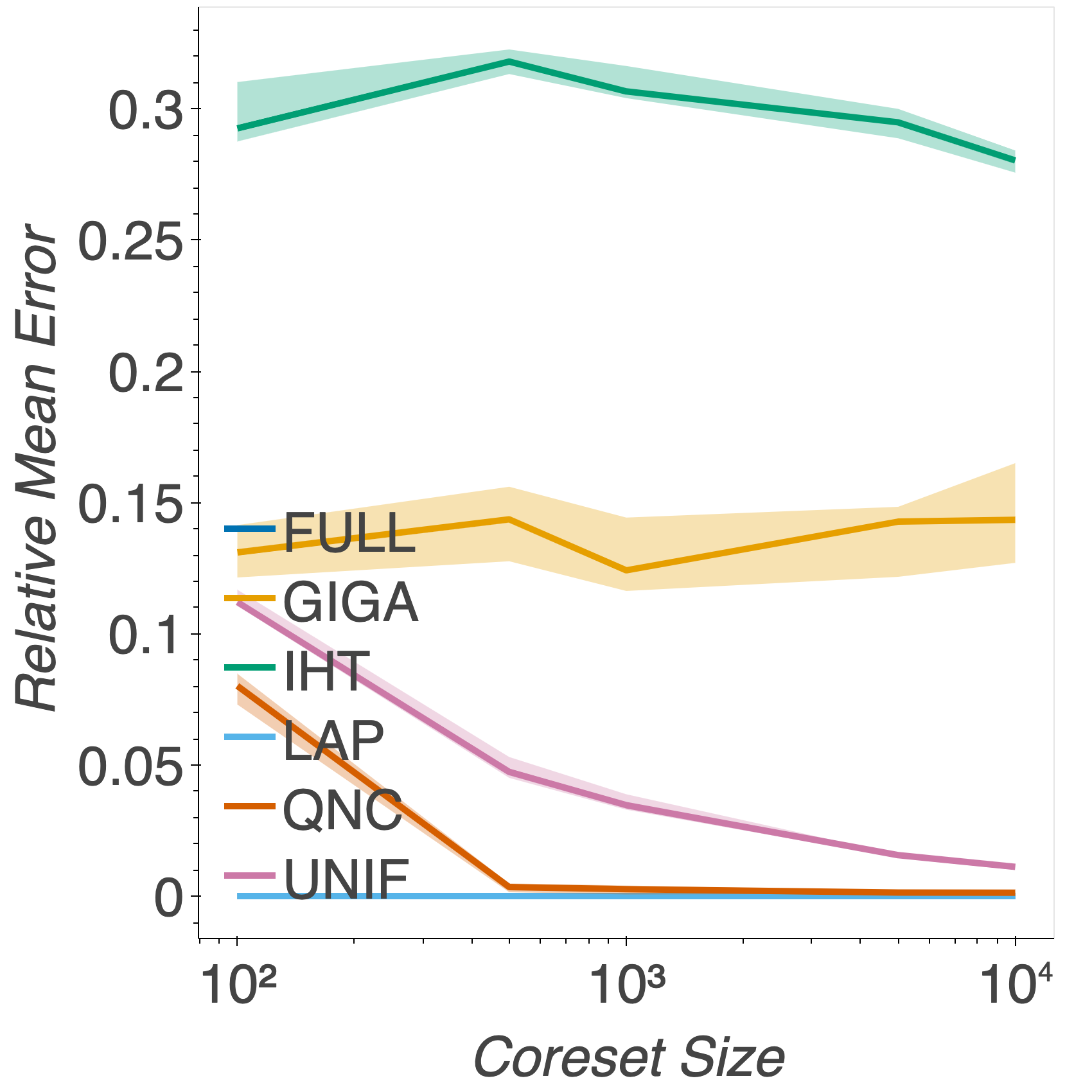
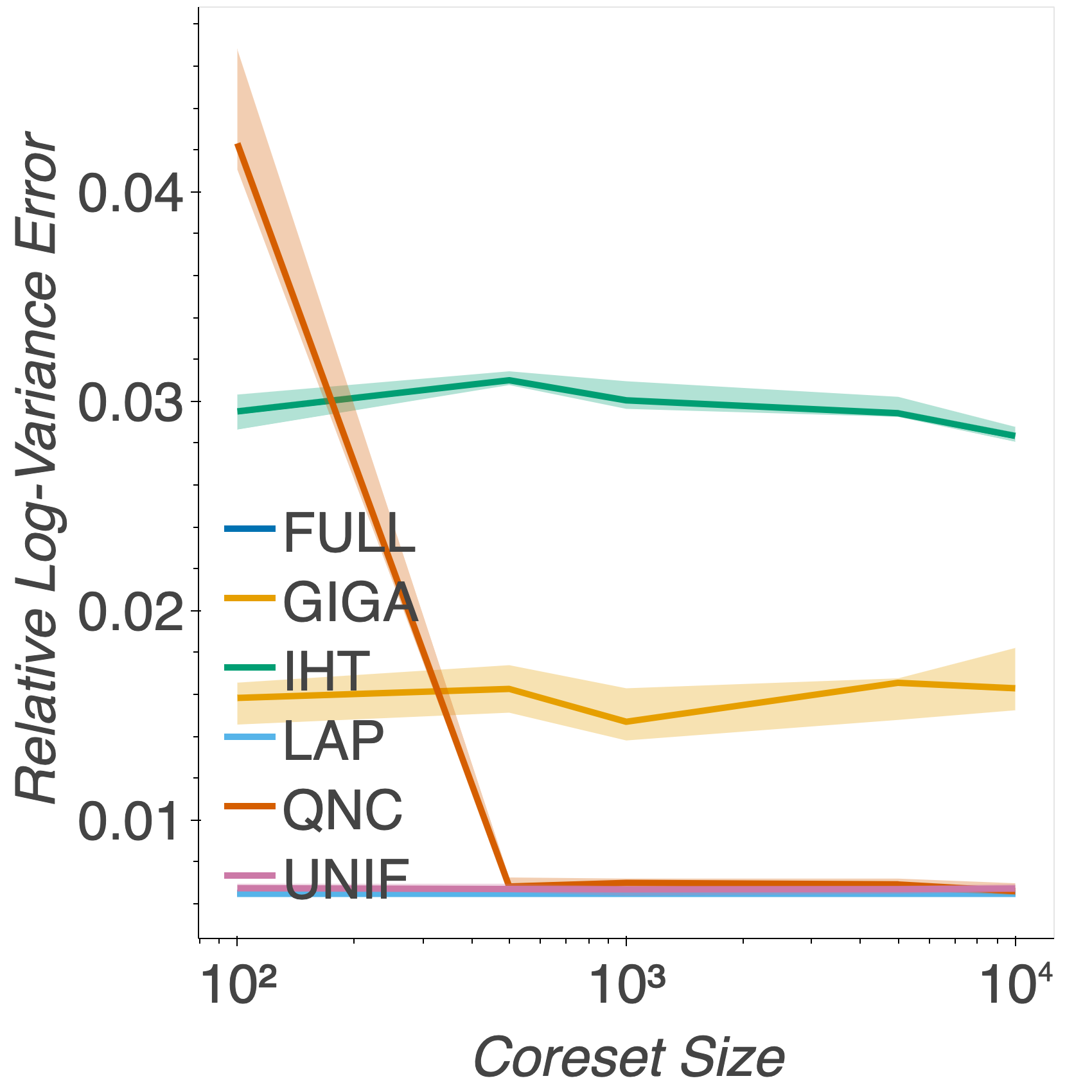
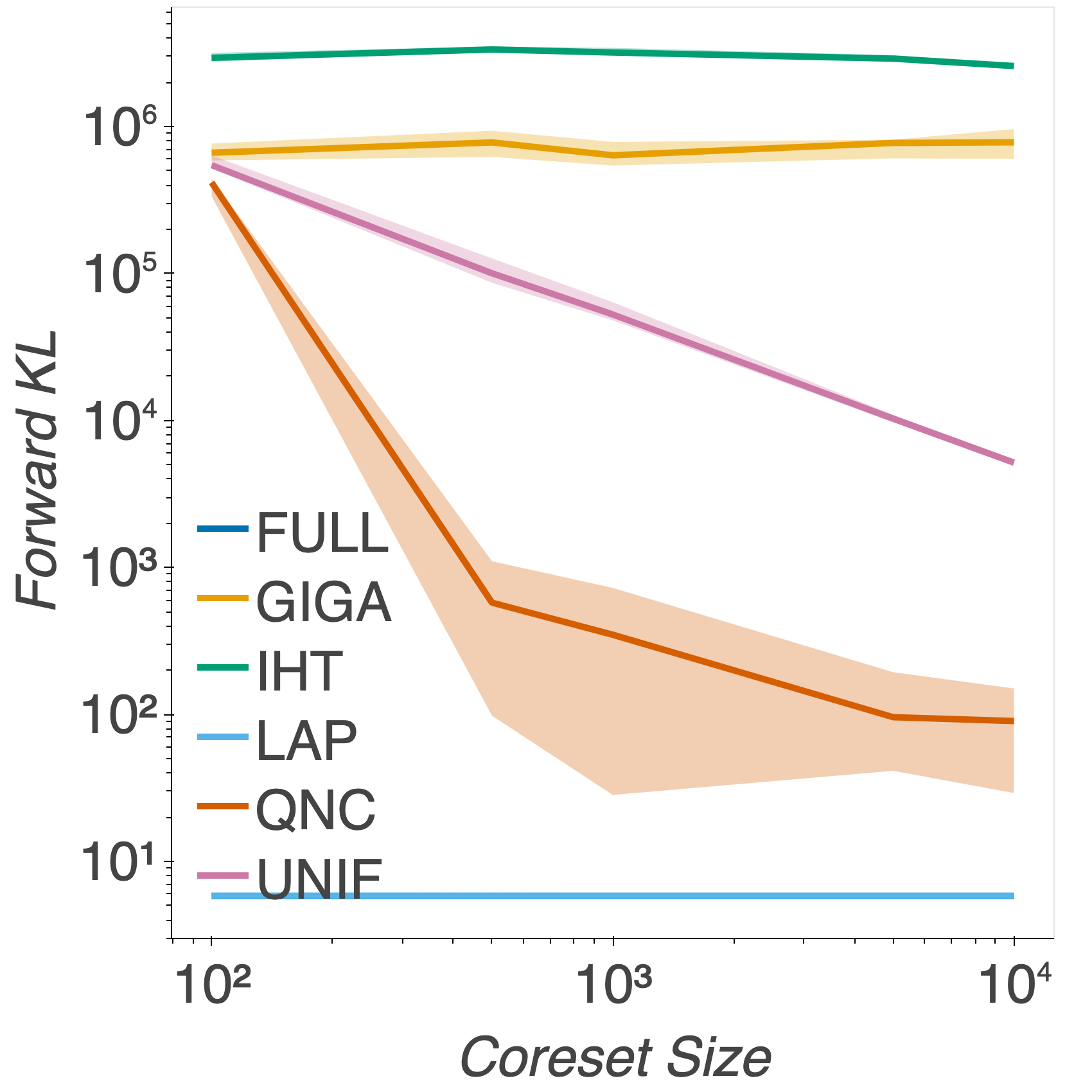
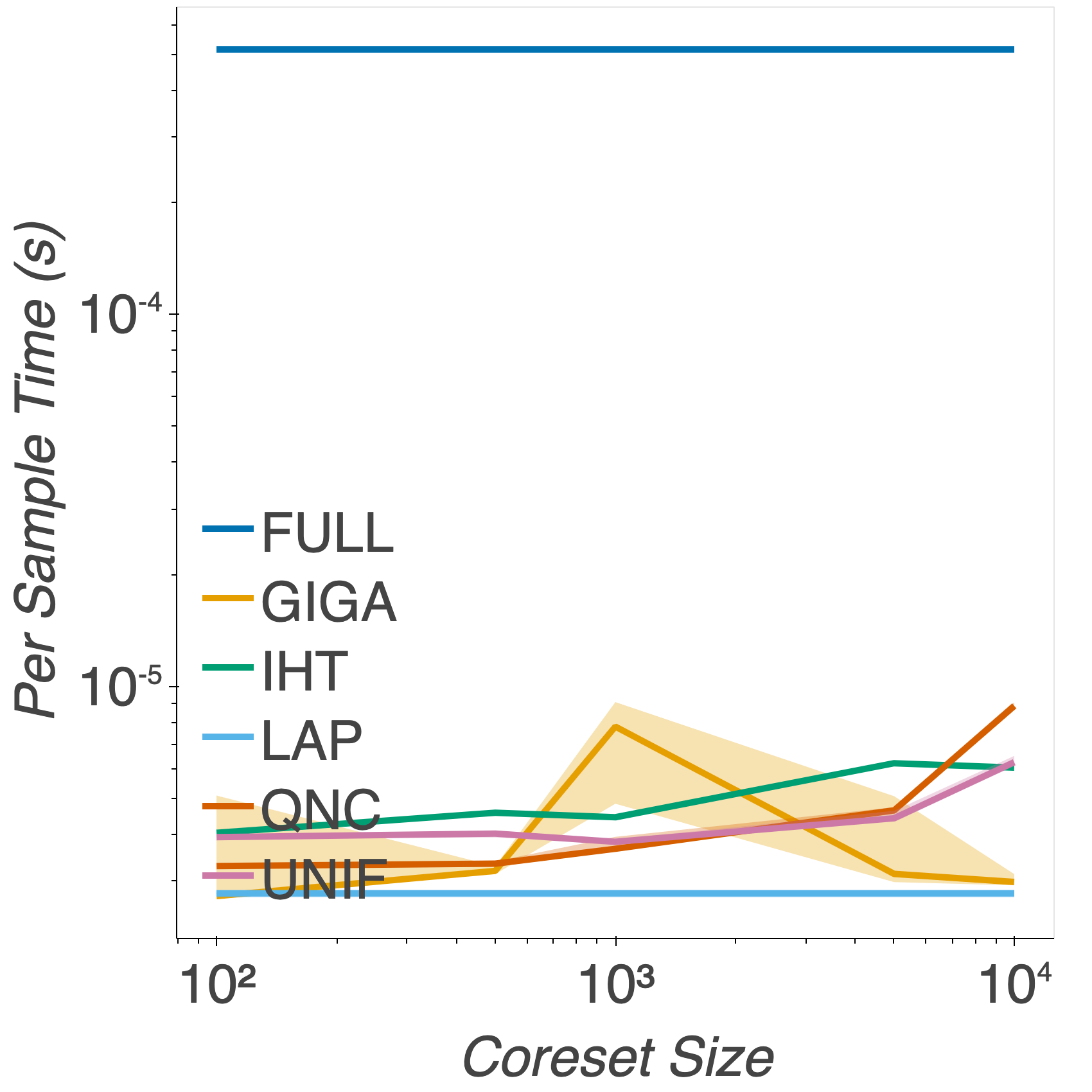
Figure 2: Relative mean and log-variance error, forward KL divergence and per sample time to sample from the respective posteriors for the synthetic Gaussian experiment. Our algorithm (QNC) consistently provides an improvement in coreset quality over the other subsampling methods. All methods provide a significant reduction in time to sample from the respective posteriors.

From Fig. 2 we see that our additional results match closely those in Section 5. Our method (QNC) consistently outperforms the other subsampling methods, while the Laplace approximation gives the best results, by design.

C.2 Bayesian sparse linear regression

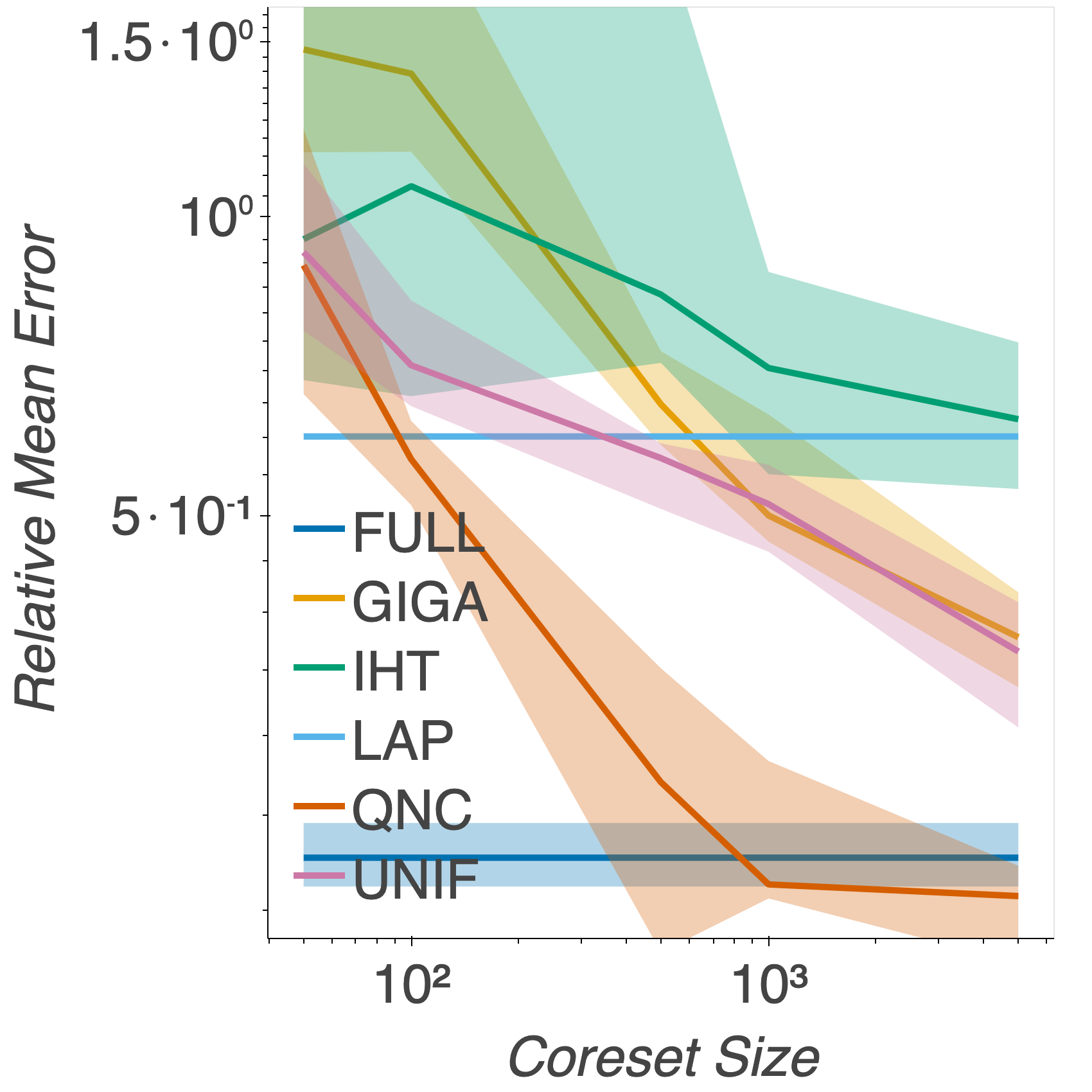
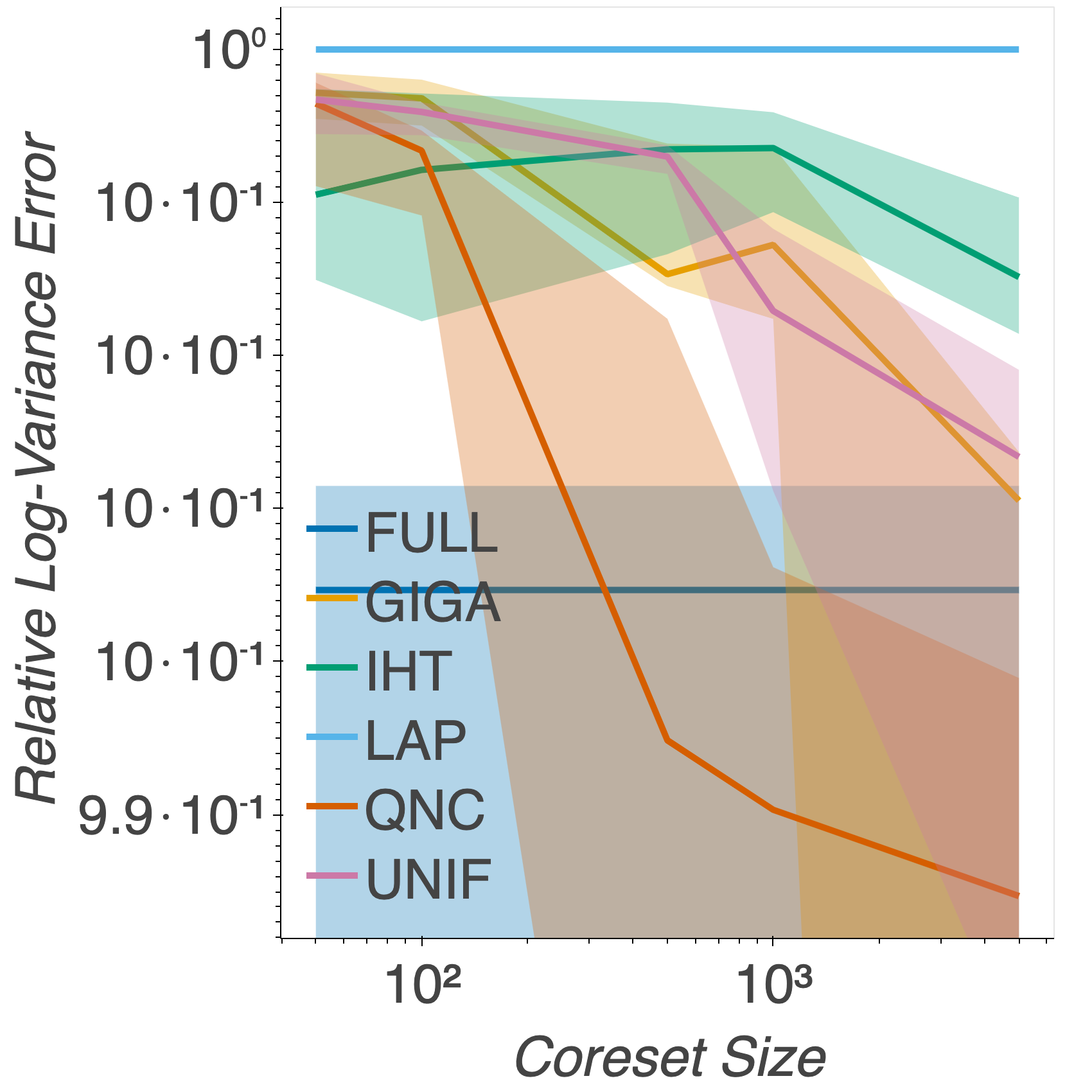
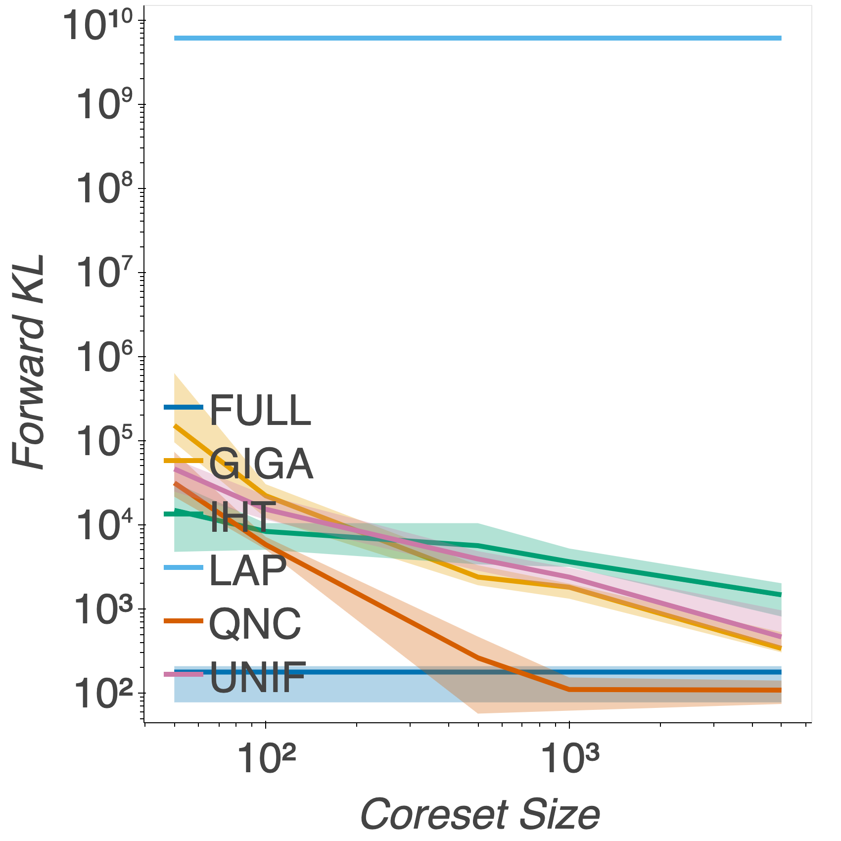
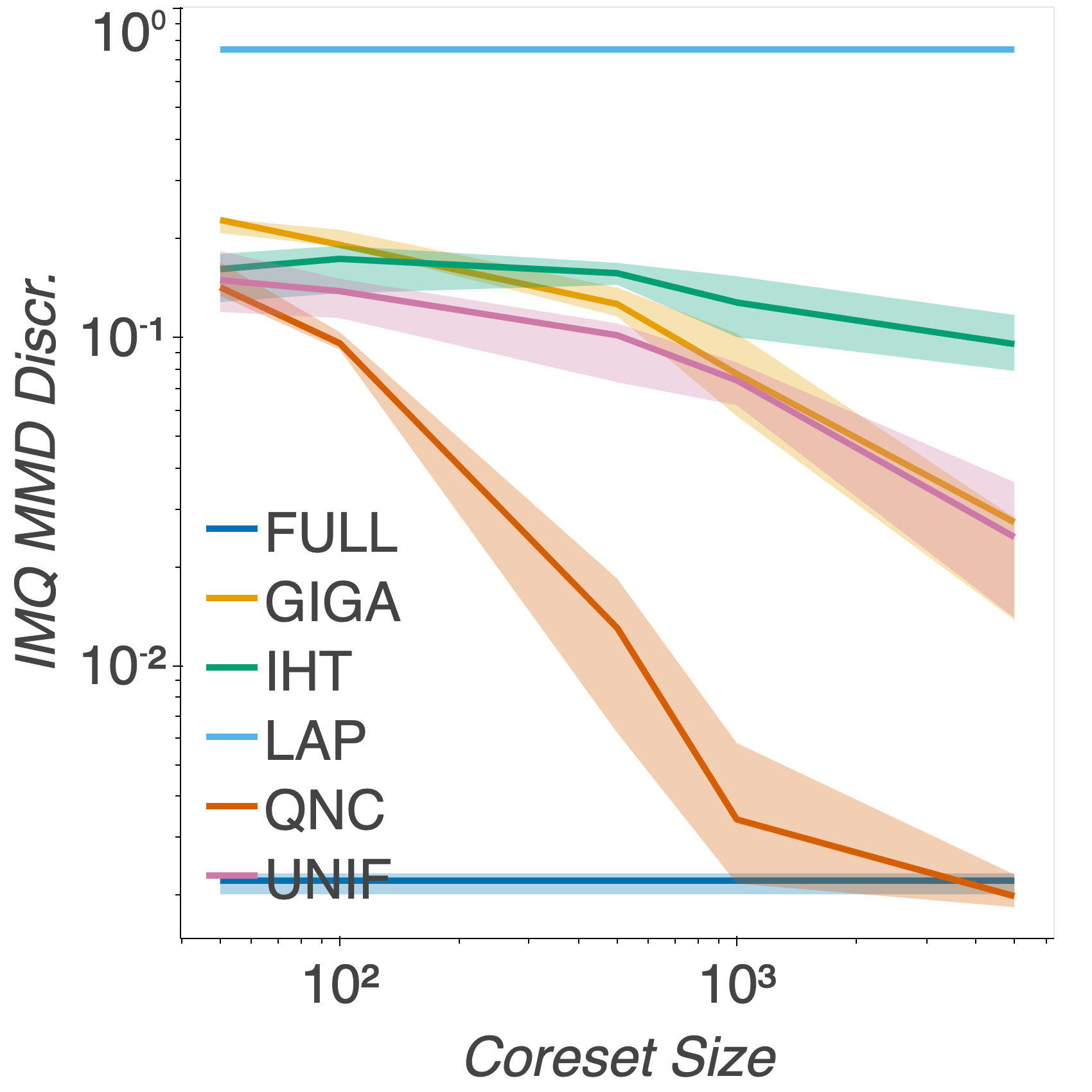
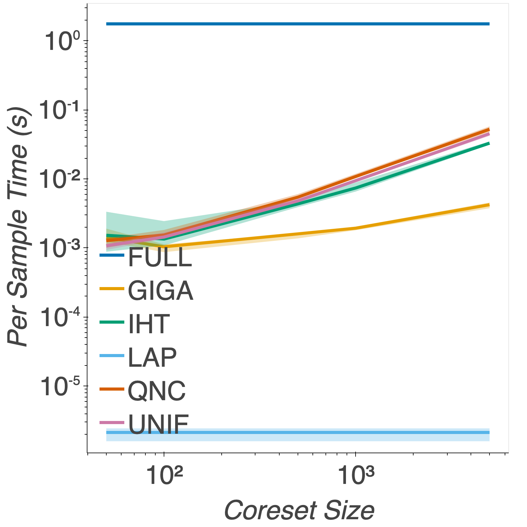
Figure 3: Relative mean and log-variance error, forward KL divergence, IMQ maximum mean discrepancy (MMD) and per sample time to sample from the respective posteriors for the sparse regression experiment. Our algorithm (QNC) consistently provides an improvement in coreset quality over the other methods. All methods provide a significant reduction in time to sample from the respective posteriors. The poor performance of the Laplace approximation in this heavy-tailed example can be seen particularly clearly in the forward KL and IMQ MMD plots.

From Fig. 3 we see that our additional results match closely those in Section 5. Our method (QNC) consistently outperforms the other methods. In order to assess the computation gains our coreset approach achieves, a useful metric is to calculate the number of posterior samples $N_{sample}$ for which the time taken to obtain $N_{sample}$ samples from the full posterior is the same as the time taken to construct a coreset using QNC, and then take $N_{sample}$ samples from the coreset posterior. Here, we find that $N_{sample}\approx 60$ for a coreset of size $1000$. This is far fewer than you would ideally like to have in practice.

However, we note that these results are conservative, and in fact we expect that the gains from the coreset approach are more significant. This is because we perform sampling in each case using STAN[31], which uses C++. However, we construct the coresets in Python, and most of the coreset build time comes from the slowness of a non-compiled language. We expect that our estimated value of $N_{sample}$ would be far smaller if we not only performed sampling in C++, but also constructed the coresets in C++.

In this experiment, the prior is heavy tailed, whilst the likelihood has sub-exponential tails. However, when the data is in fact concentrated on a particular subspace of the overall space, then the posterior can have heavy tails, even when the number of data points is large. We can clearly see this in Fig. 4, where we plot the quantiles of the (centred and scaled) marginal posterior distribution of the parameter $\lambda_{13}$ to the quantiles of a standard normal distribution. This parameter is strictly positive, but we see that the right hand tail of the distribution is significantly heavier than a normal distribution.

In the forward KL and IMQ maximum mean discrepancy (MMD) plots, we can see clearly that the Laplace approximation is performing poorly, as it is underestimating the tails of the posterior distribution. Calculating the IMQ stein discrepancy in this experiment is computationally intractable with the size of dataset we consider.

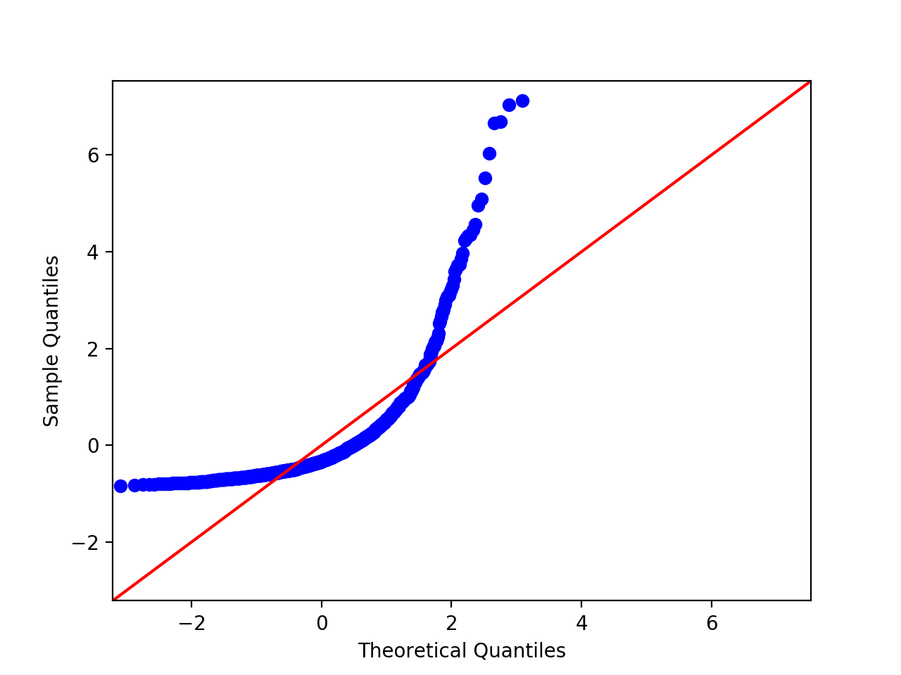
Figure 4: Quantile-quantile plot, comparing the quantiles of the (centred and scaled) marginal posterior distribution of $\lambda_{13}$ to the quantiles of a standard normal distribution.

C.3 Heavy-tailed Bayesian logistic regression

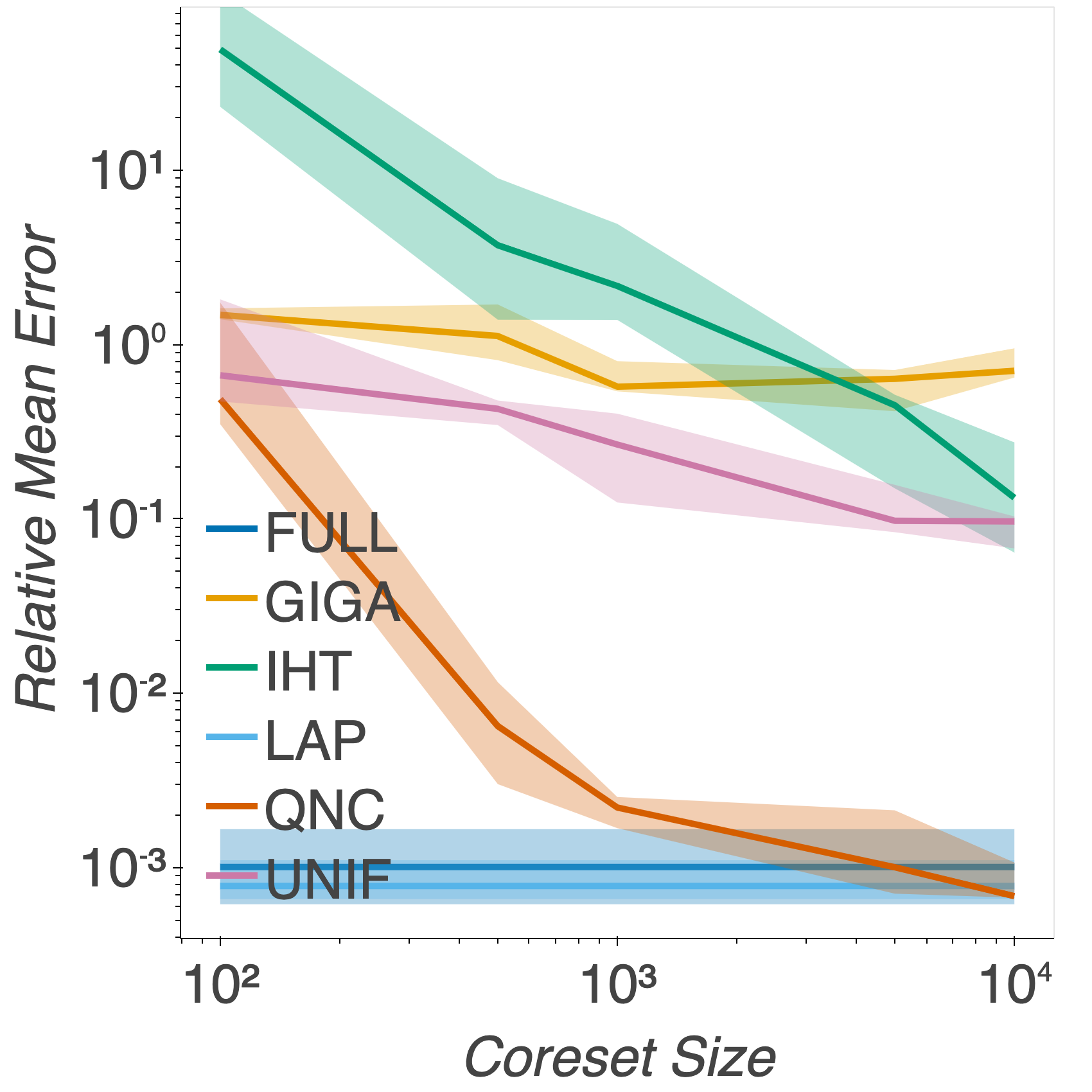
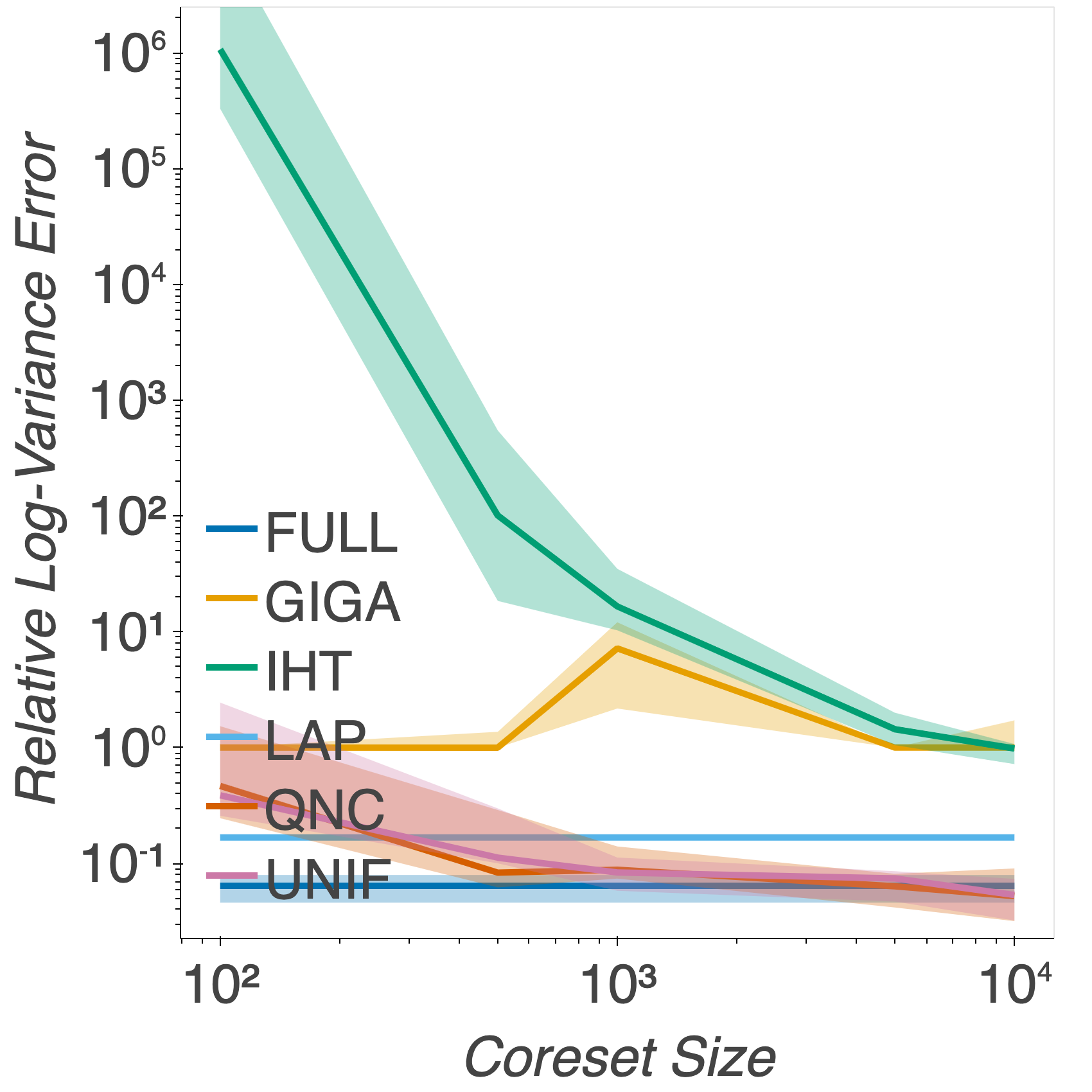
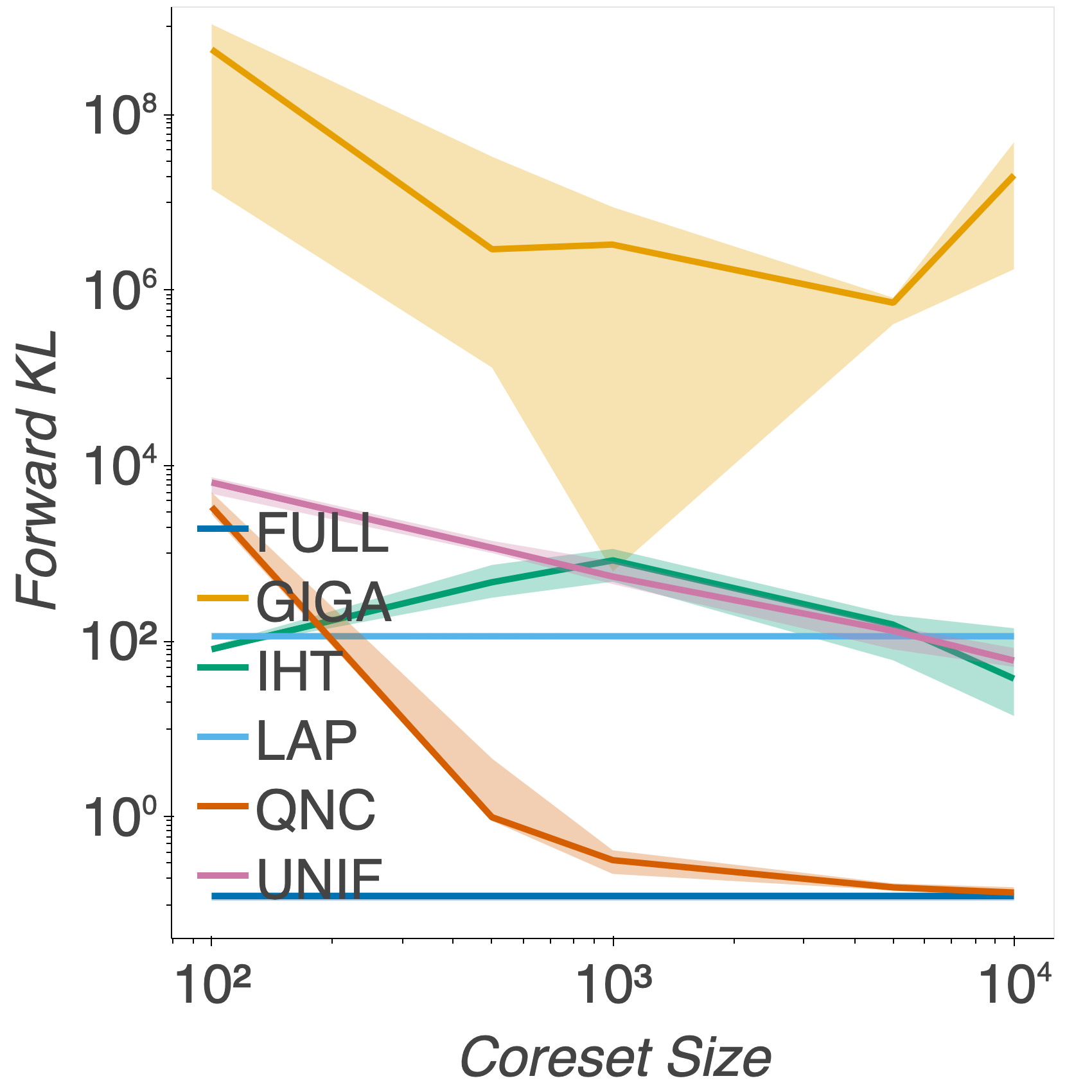
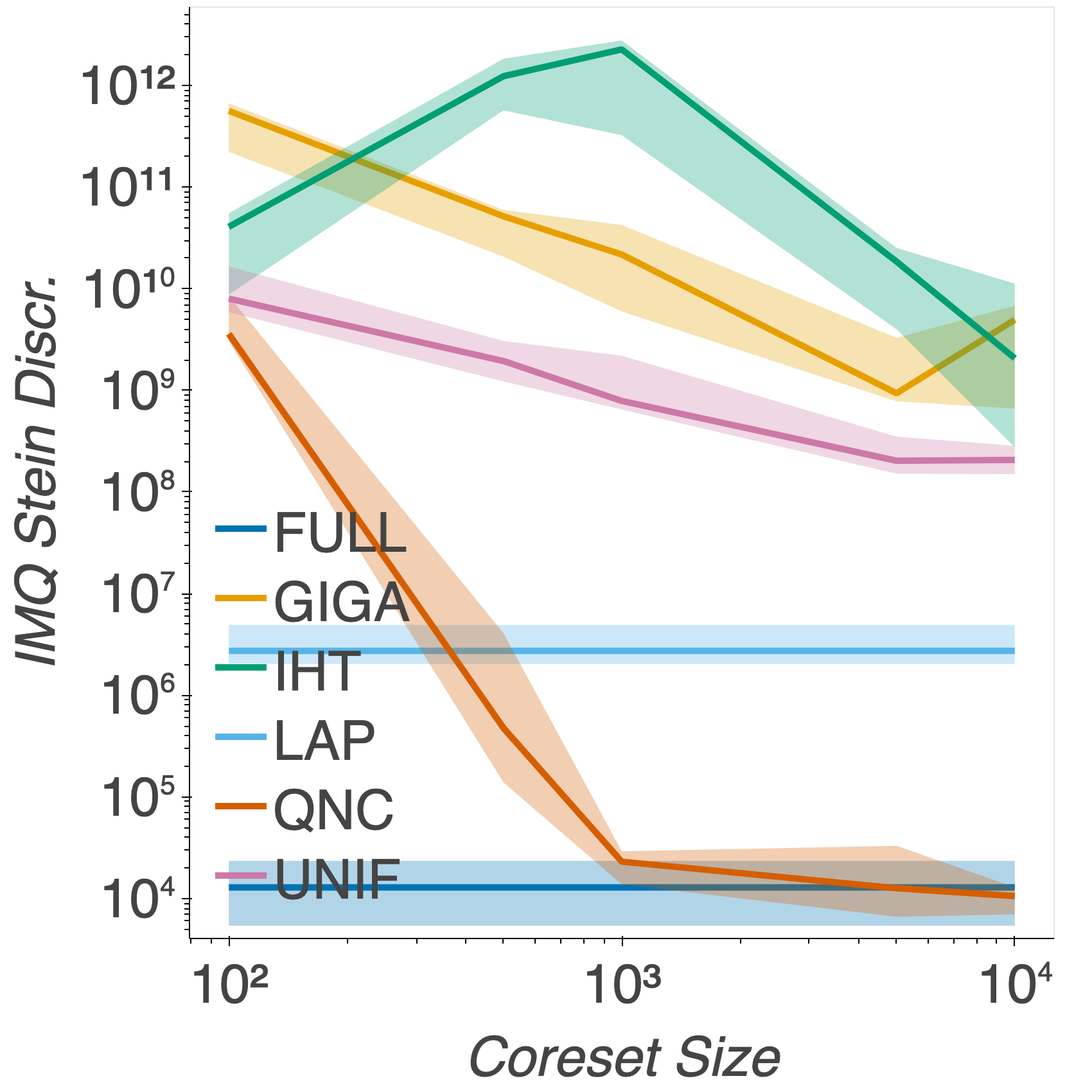
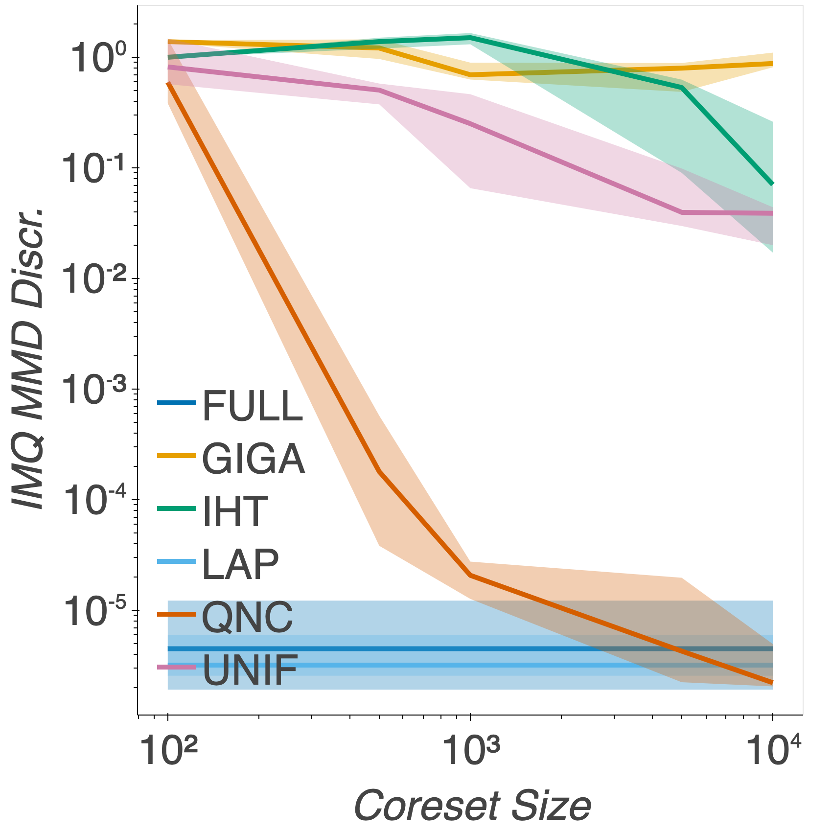
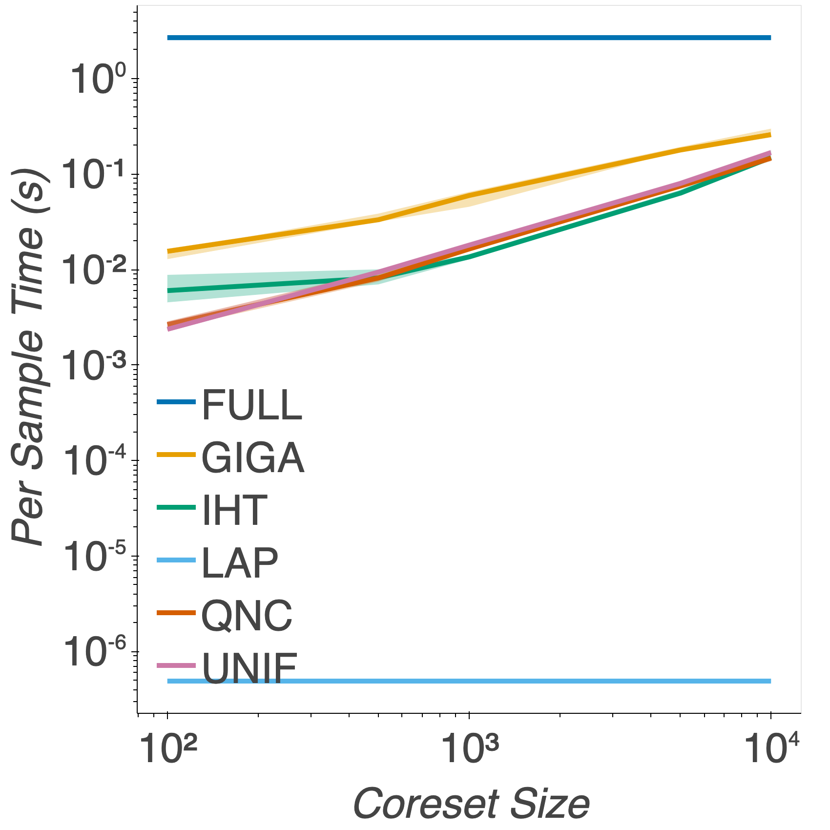
Figure 5: Relative mean and log-variance error, forward KL divergence, IMQ stein discrepancy, IMQ maximum mean discrepancy (MMD) and per sample time to sample from the respective posteriors for the logistic regression experiment. Our algorithm (QNC) generally provides an improvement in coreset quality over the other methods. All methods provide a significant reduction in time to sample from the respective posteriors.

From Fig. 5 we see that our additional results match closely those in Section 5. Our method (QNC) consistently outperforms the other methods. As before, we can calculate the number of posterior samples $N_{sample}$ for which the time taken to obtain $N_{sample}$ samples from the full posterior is the same as the time taken to construct a coreset using QNC, and then take $N_{sample}$ samples from the coreset posterior. Here, we find that $N_{sample}\approx 120$ for a coreset of size $1000$. This is again far fewer than you would ideally like to have in practice.

C.4 Bayesian radial basis function regression

Our final comparison is on a Bayesian basis function regression example, and we provide the full details of that experiment here. We perform inference for the coefficients $\alpha\in\mathbb{R}^{D}$ in a linear combination of radial basis functions $b_{k}(x)=\exp\left(-1/2\sigma_{k}^{2}\left(x-\mu_{k}\right)^{2}\right),k=1,\ldots,D$,

$$y_{n} =b_{n}^{T}\alpha+\epsilon_{n},\quad\epsilon_{n}\stackrel{{\scriptstyle\text{ i.i.d. }}}{{\sim}}\mathcal{N}\left(0,\sigma^{2}\right),\quad b_{n} =\left[\begin{array}[]{llll}b_{1}\left(x_{n}\right)&\cdots&b_{D}\left(x_{n}\right)\end{array}\right]^{T},\quad\alpha\sim\mathcal{N}\left(\mu_{0},\sigma_{0}^{2}I\right).$$

The data consists of $N=100,000$ records of house sale $\log$-price $y_{n}\in\mathbb{R}$ as a function of latitude / longitude coordinates $x_{n}\in\mathbb{R}^{2}$ in the UK. In order to perform inference we generate 50 basis functions for each of 6 scales $\sigma_{k}\in\{0.2,0.4,0.8,1.2,1.6,2.0\}$ by generating means $\mu_{k}$ uniformly from the data, and including a basis with scale 100 (i.e. nearly constant) and mean corresponding to the mean latitude and longitude of the data. Thus, we have 301 total basis functions, and so $D=301$. The prior and noise parameters $\mu_{0},\sigma_{0}^{2},\sigma^{2}$ are equal to the empirical mean, second moment, and variance of the price paid $\left(y_{n}\right)_{n=1}^{N}$ across the whole dataset, respectively. Closed form expressions are available for the subsampled posterior distributions [21, Appendix B], and we can sample from them without MCMC.

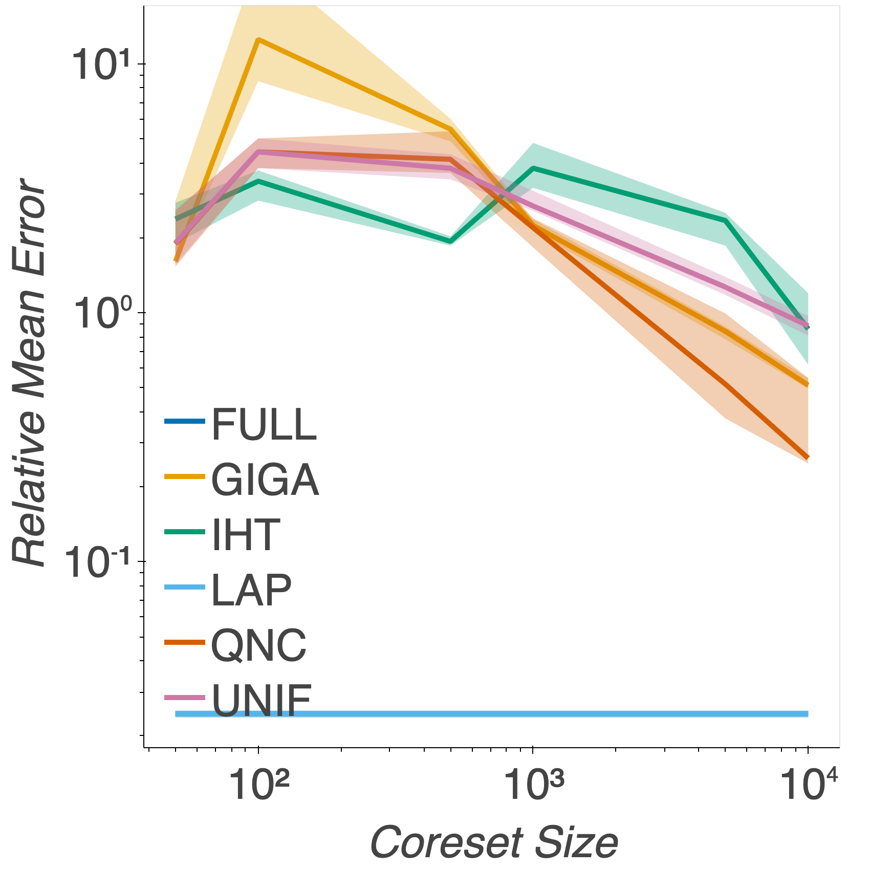
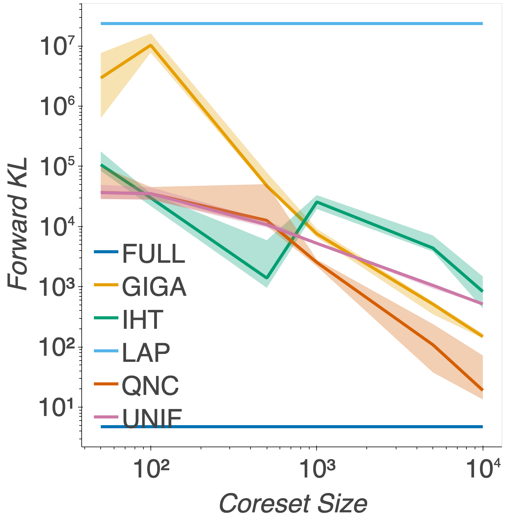
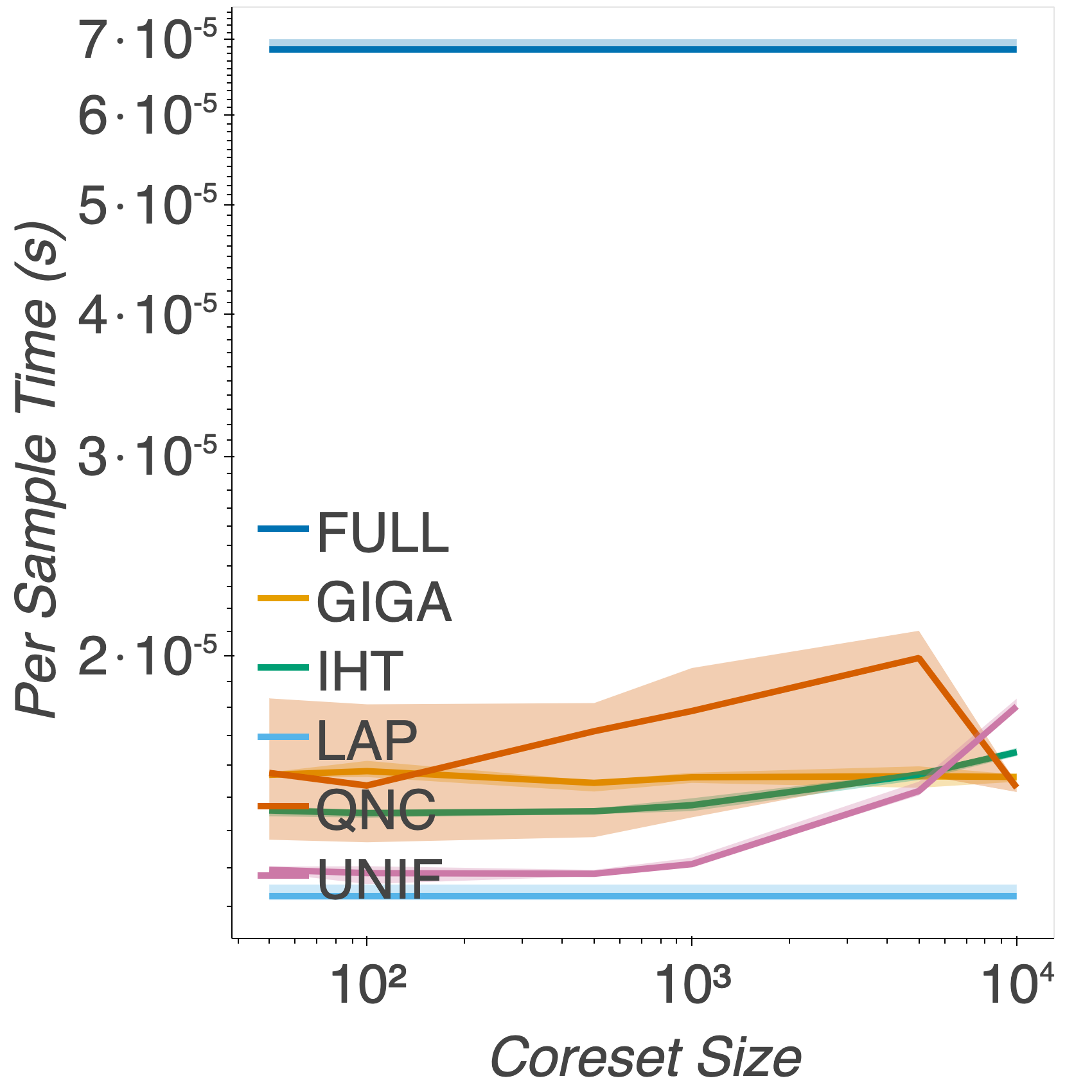
Figure 6: Relative mean and log-variance error, forward KL divergence and per sample time to sample from the respective posteriors for the basis regression experiment. Our algorithm (QNC) generally provides an improvement in coreset quality over the other methods. All methods provide a significant reduction in time to sample from the respective posteriors. The poor performance of the Laplace approximation in this high-dimensional example can be seen particularly clearly in the forward KL and log-variance plots.

From Fig. 6 we see that our additional results match closely those in Section 5. Our method (QNC) generally outperforms the other methods, but has more trouble capturing the variance of the posterior, compared to the other subsampling approaches. Though the Laplace approximation captures the mean of the posterior well, it does not approximated the variance well, leading to its overall poor performance.

C.5 Comparison with Sparse Variational Inference

In this section, we provide a comparison of our method against SVI on a smaller dataset than that used in our original experiments. This experiment is the same as that in Section 5.1, except that we have reduced the dimension from $100$ to $50$, and the dataset size from $1,000,000$ to $10,000$. For SVI we use $100$ optimization iterations, and only run 1 trial. From Fig. 7, we see that, even in this smaller data setting, the performance of SVI is not comparable. In reality, the number of optimization iterations needed is much higher than $100$, which is reflected in the poor performance. However, we see that even for this number of optimization iterations the build time can be several orders of magnitude slower than any other method. Thus, we conclude that using SVI is not feasible on the size of datasets that we consider.

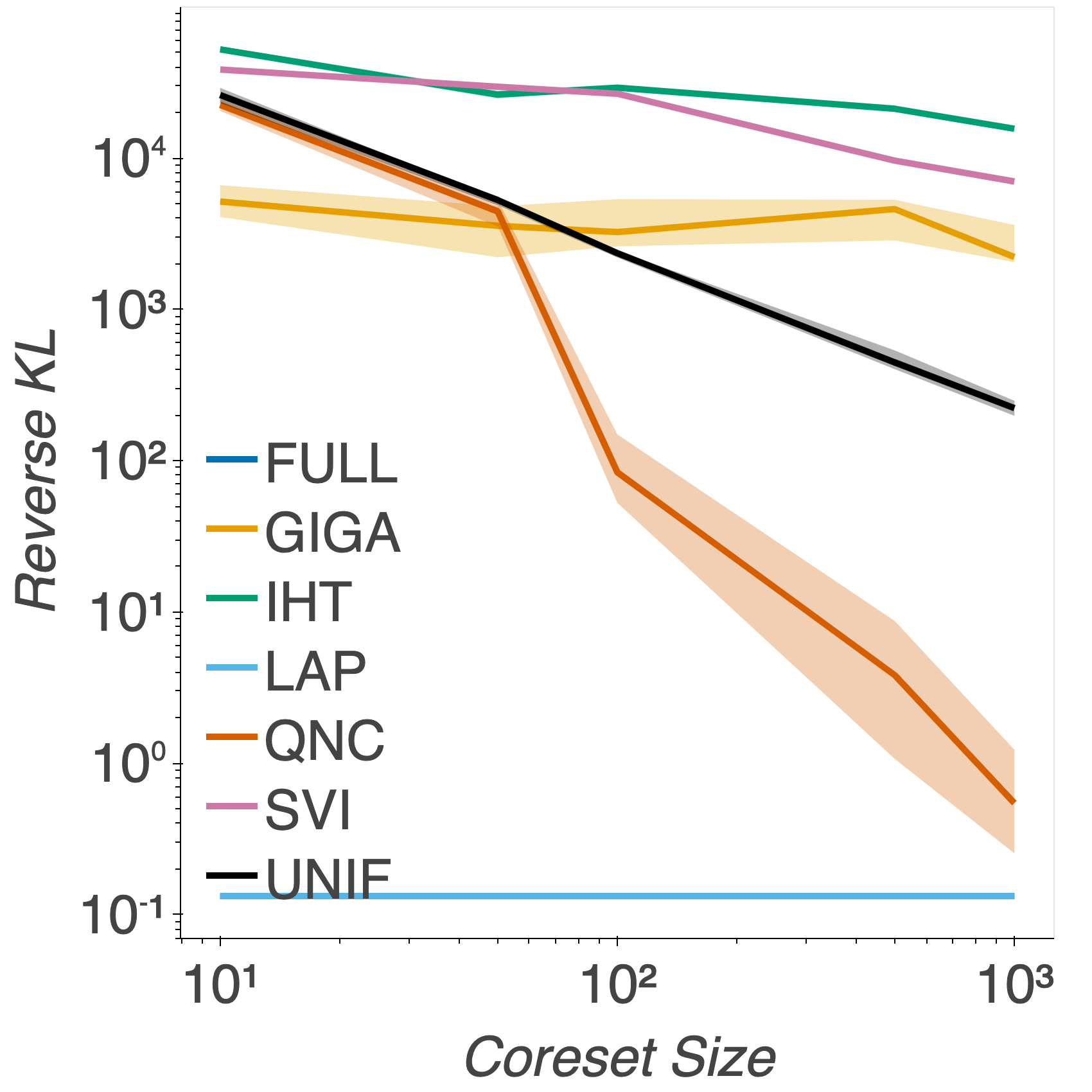
Figure 7: Reverse KL divergence (left) and build time in seconds (right) for the small synthetic Gaussian experiment.

C.6 Sparse regression methods with Laplace approximation

In Section 5, we use a uniformly sampled coreset approximation of size $M$ as the low-cost approximation $\hat{\pi}$ for GIGA and IHT. Here, we include additional results with a Laplace approximation used for $\hat{\pi}$. These are labeled as GIGA-LAP and IHT-LAP respectively.

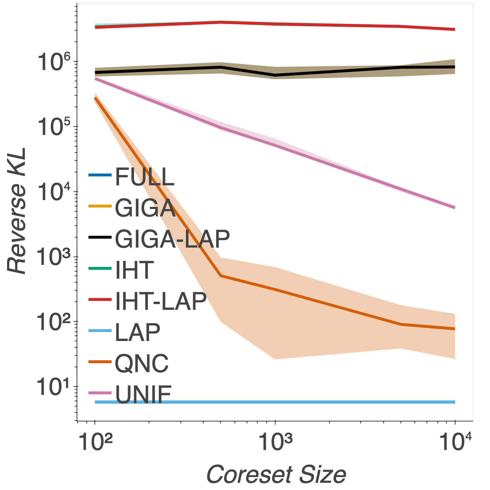
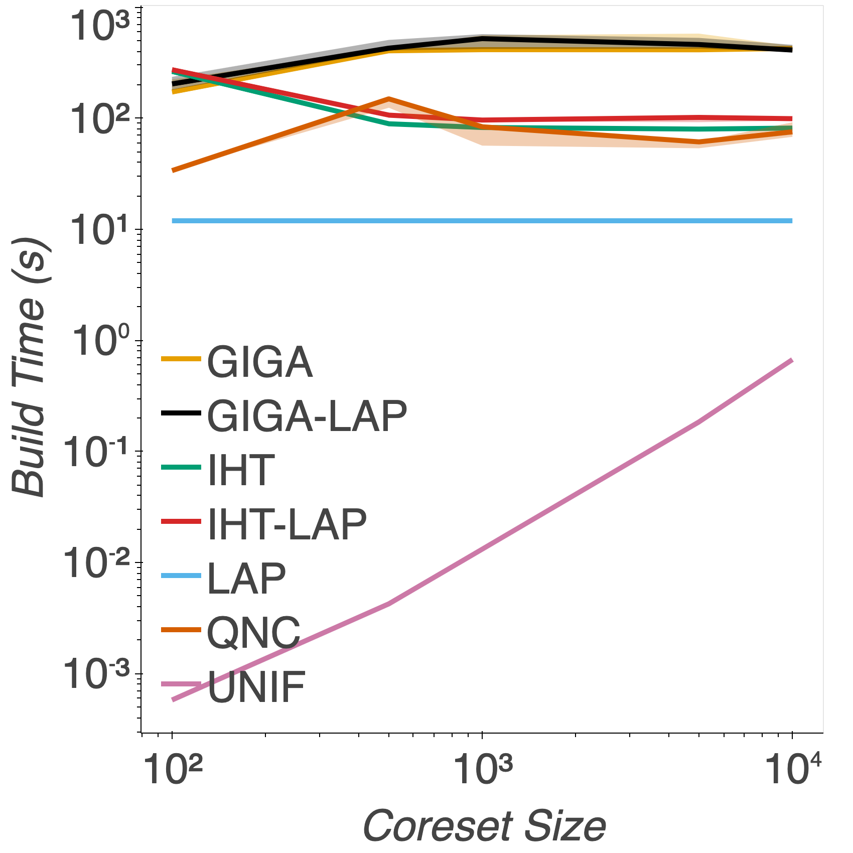
(a) Gaussian

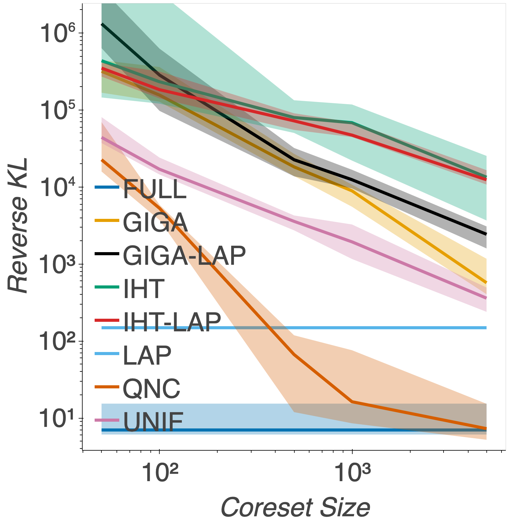
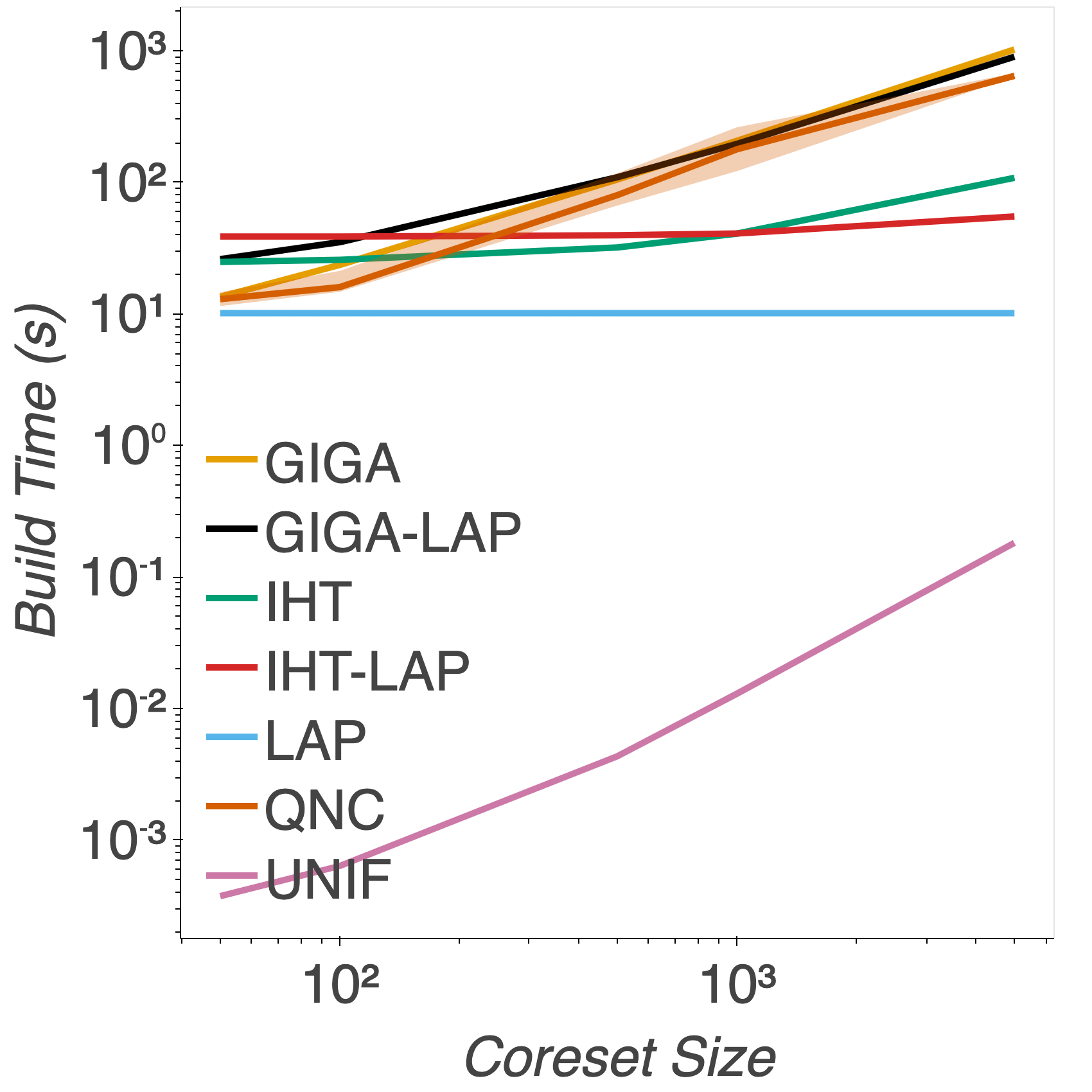
(b) Sparse linear regression

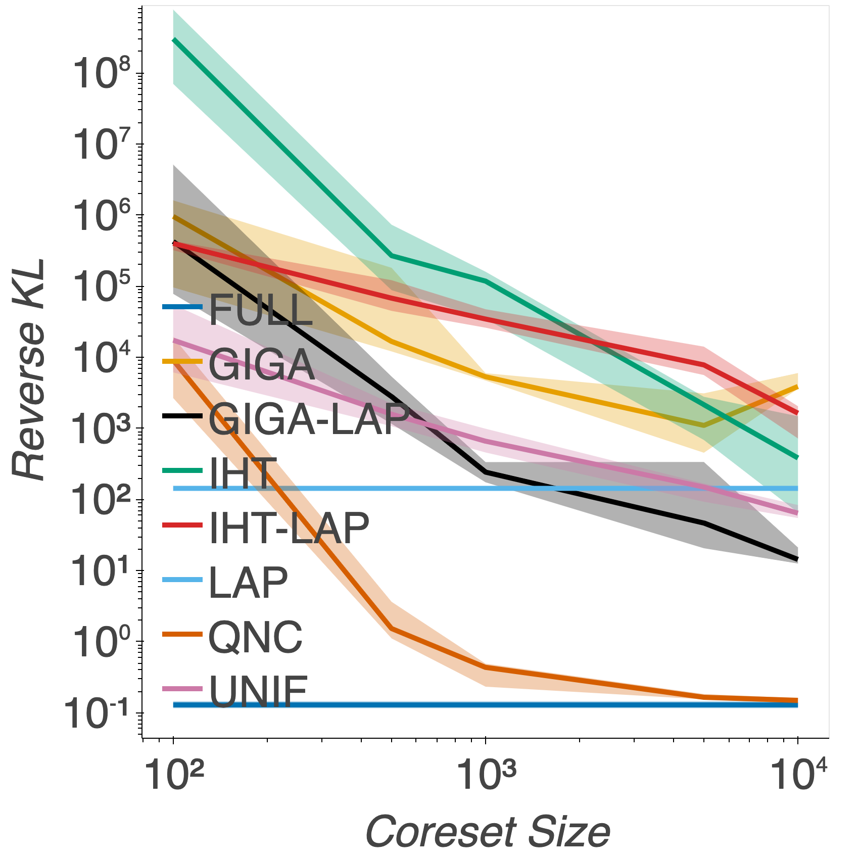
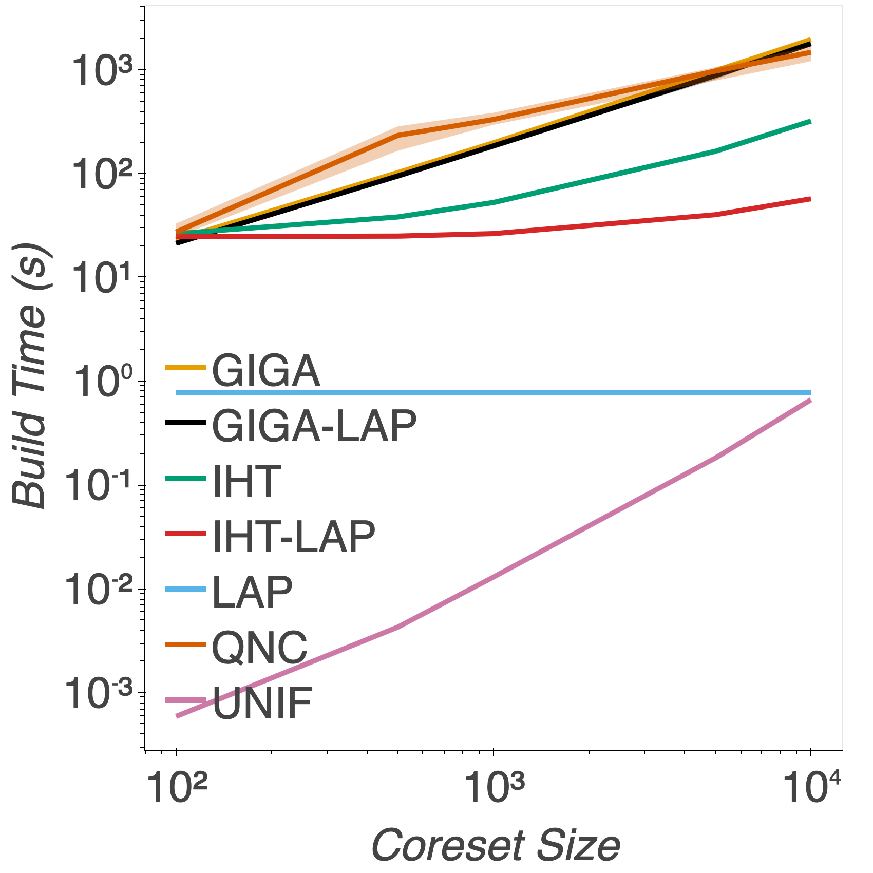
(c) Logistic regression

(d) Basis function regression

Figure 8: Reverse KL divergence (left) and build time in seconds (right) for each experiment, with added plots for GIGA and IHT with a Laplace approximation used for $\hat{\pi}$. We plot the median and a shaded area between the 25${}^{\text{th}}$/75${}^{\text{th}}$ percentiles over 10 random trials. Using a Laplace approximation used for $\hat{\pi}$ rarely provides an improvement in performance, and in some cases performs significantly worse than with the uniform choice of $\hat{\pi}$.

In Fig. 8, we see that in the synthetic Gaussian experiment, the choice of $\hat{\pi}$ has very little effect, and both GIGA and IHT perform quite badly in this large, high-dimensional example. In the sparse regression and basis function regression experiments, using a Laplace approximation for $\hat{\pi}$ leads to a worse performance. This may be unsurprising because the Laplace approximation (LAP) does not provide a good approximation to the true posterior in these settings, as detailed above and in Section 5. Only in the logistic regression experiment do we see an improvement in performance from GIGA-LAP over GIGA.

One reason for this is that the Laplace approximation provides limited help in coreset construction. Due to the large data set sizes used in our experiments, we only use a small number of samples ($S=500$) in the coreset construction process. However, especially in high dimensions, we need a large number of samples to obtain a good $L_{2}$ approximation to the posterior from the Laplace approximation.

C.7 Performance of sparse regression methods

Throughout our experiments, we see that the sparse regression methods GIGA and IHT perform poorly. One reason for this is that these methods involve approximating a high dimensional integral with a small, fixed, number of samples. This problem persists no matter which choice of low-cost approximation $\hat{\pi}$ we make, and is particularly problematic in high dimensions [34]. As noted by [21], methods like these are further limited by using a fixed approximation $\hat{\pi}$, rather than iteratively updating it as in the sparse variational inference approach.

C.8 Sensitivity Analysis

In this section we perform a sensitivity analysis for the parameters $S$, $K_{tune}$ and $\tau$ that we use in Algorithm 1. We do this by repeating the Bayesian sparse linear regression experiment detailed in Section 5.2 for varying values of one of these parameters at a time (with all other parameters kept fixed). From Fig. 9 we see the following:

• S: In our original experiments, we use $S=500$ throughout. From this analysis, we see that the performance of our method holds up for substantially lower values of $S$ (though taking $S=10$ is too low and leads to a degradation in performance). Moreover, doubling the number of samples does not lead to significantly better performance. The build time generally increases for larger $S$, as we would expect.

• $\mathbf{\tau:}$ In our original experiments, we use $\tau=0.01$ throughout. From this analysis, we see that taking too large a value of $\tau$ negatively affects the performance. This is in line with what we expect, since larger values skew the step away from a true Newton step. Our theory recommends taking $\tau$ as small as possible such that $G(w)+\tau I$ is still (numerically) invertible. Indeed, we see that decreasing $\tau$ can improve the performance of our model, though our choice still provides good results. Thus, we believe ours is a conservative choice that works well in practice.

• $\mathbf{K_{tune}:}$ In our original experiments, we use $K_{tune}=1$ throughout. In this analysis, we see that the choice of this parameter has very little effect on the performance of our method for this experiment. In our original experiments, we take $\gamma_{k}=1$ for $k>K_{tune}$. When we perform our line search, our starting value is also $\gamma_{k}=1$. We find that the line search stops immediately, meaning that for every value of $K_{tune}$ we get essentially the same results.

  The purpose of this step in our algorithm is to guard against the case where our initial gradient and covariance estimates are very noisy, and we may want to take a smaller step initially. However, we see that this is in fact not needed for this experiment.

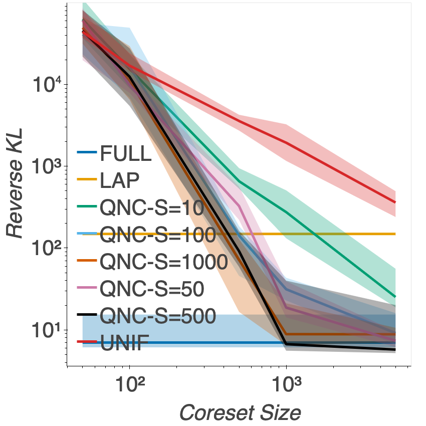
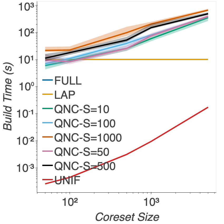
(a) S

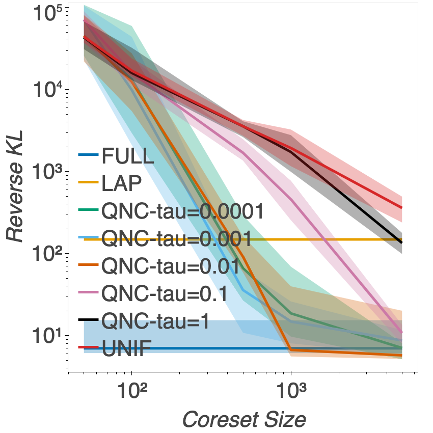
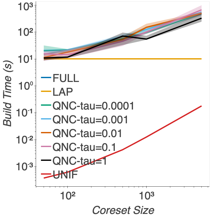
(b) $\tau$

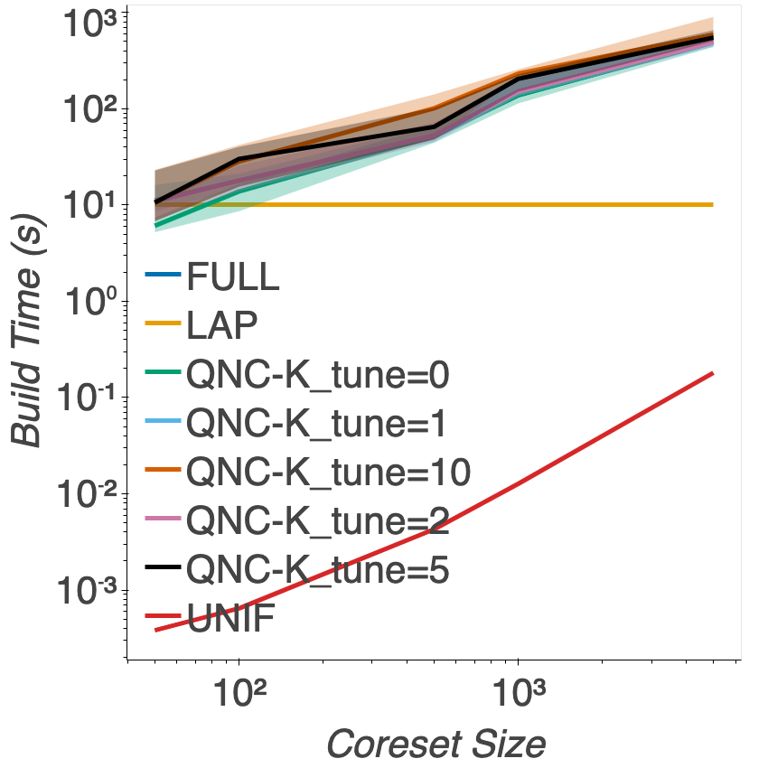
(c) $K_{tune}$

Figure 9: Sensitivity Analyses for the parameters $(a)$ $S$, $(b)$ $\tau$ and $(c)$ $K_{tune}$. In each case, we plot the Reverse KL divergence (left) and build time in seconds (right) for the sparse regression experiment.

References

• Robert and Casella [2004] Christian Robert and George Casella. Monte Carlo Statistical Methods. Springer, 2nd edition, 2004.
• Robert and Casella [2011] Christian Robert and George Casella. A short history of Markov Chain Monte Carlo: subjective recollections from incomplete data. Statistical Science, 26(1):102–115, 2011.
• Gelman et al. [2013] Andrew Gelman, John Carlin, Hal Stern, David Dunson, Aki Vehtari, and Donald Rubin. Bayesian data analysis. CRC Press, 3rd edition, 2013.
• Hoffman et al. [2013] Matthew D. Hoffman, David M. Blei, Chong Wang, and John Paisley. Stochastic variational inference. Journal of Machine Learning Research, 14:1303–1347, 2013.
• Ranganath et al. [2014] Rajesh Ranganath, Sean Gerrish, and David Blei. Black box variational inference. In International Conference on Artificial Intelligence and Statistics, 2014.
• Bardenet et al. [2017] Rémi Bardenet, Arnaud Doucet, and Chris Holmes. On Markov chain Monte Carlo methods for tall data. The Journal of Machine Learning Research, 18(1):1515–1557, 2017.
• Korattikara et al. [2014] Anoop Korattikara, Yutian Chen, and Max Welling. Austerity in MCMC land: cutting the Metropolis-Hastings budget. In International Conference on Machine Learning, 2014.
• Maclaurin and Adams [2014] Dougal Maclaurin and Ryan Adams. Firefly Monte Carlo: exact MCMC with subsets of data. In Conference on Uncertainty in Artificial Intelligence, 2014.
• Welling and Teh [2011] Max Welling and Yee Whye Teh. Bayesian learning via stochastic gradient Langevin dynamics. In International Conference on Machine Learning, 2011.
• Ahn et al. [2012] Sungjin Ahn, Anoop Korattikara, and Max Welling. Bayesian posterior sampling via stochastic gradient Fisher scoring. In International Conference on Machine Learning, 2012.
• Quiroz et al. [2018] Matias Quiroz, Robert Kohn, and Khue-Dung Dang. Subsampling MCMC—an introduction for the survey statistician. Sankhya: The Indian Journal of Statistics, 80-A:S33–S69, 2018.
• Bierkens et al. [2019] Joris Bierkens, Paul Fearnhead, and Gareth Roberts. The zig-zag process and super-efficient sampling for bayesian analysis of big data. The Annals of Statistics, 47(3):1288–1320, 2019.
• Pollock et al. [2020] Murray Pollock, Paul Fearnhead, Adam M Johansen, and Gareth O Roberts. Quasi-stationary monte carlo and the scale algorithm. Journal of the Royal Statistical Society: Series B (Statistical Methodology), 82(5):1167–1221, 2020.
• Johndrow et al. [2020] James Johndrow, Natesh Pillai, and Aaron Smith. No free lunch for approximate MCMC. arXiv:2010.12514, 2020.
• Nagapetyan et al. [2017] Tigran Nagapetyan, Andrew Duncan, Leonard Hasenclever, Sebastian Vollmer, Lukasz Szpruch, and Konstantinos Zygalakis. The true cost of stochastic gradient Langevin dynamics. arXiv:1706.02692, 2017.
• Betancourt [2015] Michael Betancourt. The fundamental incompatibility of Hamiltonian Monte Carlo and data subsampling. In International Conference on Machine Learning, 2015.
• Quiroz et al. [2019] Matias Quiroz, Robert Kohn, Mattias Villani, and Minh-Ngoc Tran. Speeding up MCMC by efficient data subsampling. Journal of the American Statistical Association, 114(526):831–843, 2019.
• Huggins et al. [2016] Jonathan Huggins, Trevor Campbell, and Tamara Broderick. Coresets for scalable Bayesian logistic regression. In Advances in Neural Information Processing Systems, 2016.
• Campbell and Broderick [2019] Trevor Campbell and Tamara Broderick. Automated scalable Bayesian inference via Hilbert coresets. Journal of Machine Learning Research, 20(15), 2019.
• Campbell and Broderick [2018] Trevor Campbell and Tamara Broderick. Bayesian coreset construction via greedy iterative geodesic ascent. In International Conference on Machine Learning, 2018.
• Campbell and Beronov [2019] Trevor Campbell and Boyan Beronov. Sparse variational inference: Bayesian coresets from scratch. In Advances in Neural Information Processing Systems, 2019.
• Manousakas et al. [2020] Dionysis Manousakas, Zuheng Xu, Cecilia Mascolo, and Trevor Campbell. Bayesian pseudocoresets. In Advances in Neural Information Processing Systems, 2020.
• Zhang et al. [2021] Jacky Zhang, Rajiv Khanna, Anastasios Kyrillidis, and Oluwasanmi Koyejo. Bayesian coresets: revisiting the nonconvex optimization perspective. In Artificial Intelligence in Statistics, 2021.
• Jankowiak and Phan [2021] Martin Jankowiak and Du Phan. Surrogate likelihoods for variational annealed importance sampling. arXiv preprint arXiv:2112.12194, 2021.
• Chen et al. [2022] Naitong Chen, Zuheng Xu, and Trevor Campbell. Bayesian inference via sparse hamiltonian flows. arXiv preprint arXiv:2203.05723, 2022.
• Broyden [1972] Charles Broyden. Quasi-Newton methods. In W Murray, editor, Numerical Methods for Unconstrained Optimization, pages 87–106. Academic Press, 1972.
• Wolfe [1969] Philip Wolfe. Convergence conditions for ascent methods. SIAM review, 11(2):226–235, 1969.
• Gretton et al. [2012] Arthur Gretton, Karsten M Borgwardt, Malte J Rasch, Bernhard Schölkopf, and Alexander Smola. A kernel two-sample test. The Journal of Machine Learning Research, 13(1):723–773, 2012.
• Liu et al. [2016] Qiang Liu, Jason Lee, and Michael Jordan. A kernelized Stein discrepancy for goodness-of-fit tests. In International conference on machine learning, pages 276–284. PMLR, 2016.
• Korba et al. [2021] Anna Korba, Pierre-Cyril Aubin-Frankowski, Szymon Majewski, and Pierre Ablin. Kernel Stein discrepancy descent. arXiv preprint arXiv:2105.09994, 2021.
• Carpenter et al. [2017] Bob Carpenter, Andrew Gelman, Matthew D Hoffman, Daniel Lee, Ben Goodrich, Michael Betancourt, Marcus Brubaker, Jiqiang Guo, Peter Li, and Allen Riddell. Stan: A probabilistic programming language. Journal of statistical software, 76(1):1–32, 2017.
• Amari [2016] Shun-ichi Amari. Information geometry and its applications, volume 194. Springer, 2016.
• Böröczky and Wintsche [2003] Károly Böröczky and Gergely Wintsche. Covering the sphere by equal spherical balls. In Boris Aronov, Saugata Basu, János Pach, and Micha Sharir, editors, Discrete and Computational Geometry, volume 25 of Algorithms and Combinatorics, pages 235–251. Springer, 2003.
• James et al. [2013] Gareth James, Daniela Witten, Trevor Hastie, and Robert Tibshirani. An introduction to statistical learning, volume 112. Springer, 2013.