Computing confined elasticae

Abstract.

A numerical scheme for computing arc-length parametrized curves of low bending energy that are confined to convex domains is devised. The convergence of the discrete formulations to a continuous model and the unconditional stability of an iterative scheme are addressed. Numerical simulations confirm the theoretical results and lead to a classification of observed optimal curves within spheres.

1. Introduction

Equilibrium configurations of thin elastic rods have been of interest since the times of Euler. The mathematical modelling of these deformable structures has been reduced from three dimensions to a one-dimensional problem for the center-line of the rod $u:I\to\mathbb{R}^{3}$, cf. [31, 28, 21, 36, 8]. In the bending regime, the rod is inextensible so that $|u^{\prime}|=1$ holds on $I$. Considering a circular cross section and omitting twist contributions, the elastic energy reduces to the functional

$$E_{\text{bend}}[u]=\frac{\kappa}{2}\int_{I}|u^{\prime\prime}(x)|^{2}\,{\mathrm{d}}x$$

for a parameter $\kappa>0$ that describes the bending rigidity. Elasticae, i.e. rods of minimal bending energy, can be stated explicitly e.g. for periodic boundary conditions [33, 32]. Applications of elastic thin rods include DNA modelling [42, 26, 1], the movement of actin filaments in cells [35] or of thin microswimmers [40], the fabrication of textiles [29], and investigating the reach of a rod injected into a cylinder [37].

To obtain minimally bent elastic rods, the bending energy can be reduced by a gradient-flow approach. This method can be used for analytic considerations, cf. for instance [32, 25, 38, 18, 41] and numerical computations [20, 3, 19, 4, 6, 7, 44, 13, 5, 2, 24, 14]. An efficient finite-element approach with an accurate treatment of the inextensibility condition can be used to find equilibria of free elastic rods [7] and self-avoiding rods [12, 13]. It can also be generalized to include twist contributions defined via torsion quantities [11]. We follow common conventions and refer to rods as elastic curves when twist contributions are omitted.

In this manuscript, a generalization of the existing scheme to calculate elasticae of confined elastic curves is proposed. Confinements of elastic structures arise on a variety of length scales, such as DNA plasmids or biopolymers inside a cell or chamber [17, 39]. The boundary of closely packed elastic sheets or a wire in a container can be modelled as confined elastic rods in two dimensions [22, 15]. A planar setting has been assessed in terms of phase-field modelling [23, 45]; a numerical scheme for thick elastic curves in containers is devised in [43].

We propose an approach that can be used for rods embedded in arbitrary dimensions confined to convex domains. For the mathematical modelling, we use a gradient flow to minimize the bending energy. The admissible rod configurations during the flow are restricted to a domain $D\subset\mathbb{R}^{3}$.

The task to unbend a rod inside $D$ can be translated to minimizing $E_{\text{bend}}$ among all

$$u\in\mathcal{A}\cap D,\quad\mathcal{A}=\{v\in H^{2}(I;\mathbb{R}^{3})\,:|v^{\prime}|=1\text{ a.e.},\,L_{\text{bc}}(v)=\ell_{\text{bc}}\}.$$

The bounded linear operator $L_{\text{bc}}:H^{2}(I;\mathbb{R}^{3})\to\mathbb{R}^{\ell}$ realizes appropriate boundary conditions. We restrict our considerations to those subsets $D$ that can be written as finite intersections of simple quadratic confinements $D_{r}$, $r=1,2,\dots,R$, i.e.,

$$D=\cap_{r=1}^{R}D_{r},\quad D_{r}=\{y\in\mathbb{R}^{3}:|y|_{D_{r}}^{2}=y\cdot G_{D_{r}}y\leq 1\}$$

for symmetric positive semi-definite matrices $G_{D_{r}}\in\mathbb{R}^{3\times 3}$. We call the finite intersection a composite quadratic confinement. For ease of presentation we often consider one set $D_{r}$ and then omit the index $r$. Some basic simple quadratic confinements are the ball with radius $R$ and $G_{D}=I_{3}/R^{2}$, the ellipsoid with radii $R_{1},R_{2},R_{3}$ and $(G_{D})_{ij}=\delta_{ij}/R_{i}^{2}$, or the space between two parallel planes with distance $2R$ with normal vector $n$ and $G_{D}=nn^{t}/R^{2}$. Boxes and finite cylinders can be constructed as composite quadratic confinements. In general, any simple or composite quadratic confinement is a convex, closed, and connected set.

We enforce the confinement via a potential approach, so a non-negative term is added to the bending energy whenever the curve violates the confining restrictions. We define a potential $V_{D}:\mathbb{R}^{3}\to\mathbb{R}$ for a simple quadratic confinement $D$ that vanishes in $D$ and is strictly positive on $\mathbb{R}^{3}\backslash D$ via

$$V_{D}(y)=\frac{1}{2}\left(|y|_{D}-1\right)_{+}^{2}=\frac{1}{2}|y|_{D}^{2}+\frac{1}{2}V_{D}^{\text{cv}}(y),$$

where the concave part $V_{D}^{\text{cv}}$ is given by the continuous function

$$V_{D}^{\text{cv}}(y)=\begin{cases}-|y|_{D}^{2},&\text{ if $y\in D$,}\\ -2|y|_{D}+1&\text{ else.}\end{cases}.$$

The potential is used to define a penalizing confinement energy functional

$$E_{D}[u]=\int_{I}|u(x)|_{D}^{2}+V_{D}^{\text{cv}}(u(x))\,{\mathrm{d}}x,$$

which is by the definition of the potential non-negative and zero if and only if the curve entirely lies within $D$. For a composite confinement defined via a family $(D_{r})_{r=1,\dots,R}$ of simple quadratic confinements we sum the corresponding confinement energies up, i.e.,

(1) $$E_{D}[u]=\sum_{r=1}^{R}E_{D_{r}}[u],\quad V_{D}(y)=\sum_{r=1}^{R}V_{D_{r}}(y).$$

We remark that translated domains and half-spaces, e.g., $D=\{y\in\mathbb{R}^{3}:|y-y_{D}|_{D}^{2}\leq 1\}$ and $D=\{y\in\mathbb{R}^{3}:a_{D}\cdot y\leq 1\}$ can be similarly treated.

Given $\varepsilon>0$, a curve $u_{\varepsilon}\in\mathcal{A}$ is called a (approximately) confined elastica if it is stationary for the functional

$$E_{\varepsilon}[u]=E_{\text{bend}}[u]+\frac{1}{2\varepsilon}E_{D}[u]$$

in the set $\mathcal{A}$. If $V_{D}(u_{\varepsilon})=0$ almost everywhere on $I$, the rod is called exactly confined elastica. The parameter $\varepsilon$ determines the steepness of the quadratic well potential and defines a length-scale for the penetration depth of the curve into the space outside of $D$.

Considering a simple quadratic confinement $D\subset\mathbb{R}^{3}$, we let $V_{D}\in C^{1}(\mathbb{R}^{3};\mathbb{R})$ be the corresponding quadratic-well potential, and choose $\varepsilon>0$. Trajectories $u\in H^{1}([0,T];L^{2}(I;\mathbb{R}^{3}))\cap L^{\infty}([0,T];\mathcal{A})$ are defined by gradient flow evolutions. In particular, for an inner product $(\cdot,\cdot)_{\star}$ on $L^{2}(I;\mathbb{R}^{3})$ and an initial configuration $u(0,x)=u_{0}(x)$, we define the temporal evolution as the solution of the time-dependent nonlinear system of partial differential equations

(2) $$\begin{split}(\partial_{t}u,v)_{\star}+\kappa(u^{\prime\prime},v^{\prime\prime})&+\varepsilon^{-1}(u,G_{D}v)\\ &=-(2\varepsilon)^{-1}(\nabla V_{D}^{\text{cv}}(u),v)-(\lambda u^{\prime},v^{\prime})\end{split}$$

for test functions $v\in\mathcal{V}$ with a suitable set $\mathcal{V}$ and all $t\in[0,T]$. The function $\lambda\in L^{1}([0,T]\times I)$ is a Lagrange multiplier associated with the arc-length condition. Confined elasticae are stationary points for (2).

For time discretization, we use backward differential quotients. Let $\tau>0$ be the fixed time-step and let $k\geq 0$ be a non-negative integer. We set $u^{0}:=u_{0}$ and define the time-step

$$d_{t}u^{k+1}=\frac{u^{k+1}-u^{k}}{\tau}.$$

The gradient flow system is evaluated implicitly except for the concave confinement energy, which is handled explicitly due to its non-linearity and anti-monotonicity, and the Lagrange multiplier term, which is treated semi-implicitly. We hence have

(3) $$\begin{split}(d_{t}u^{k+1},v)_{\star}+\kappa([u^{k+1}]^{\prime\prime},v^{\prime\prime})&+\varepsilon^{-1}(u^{k+1},G_{D}v)\\ &=-(2\varepsilon)^{-1}(\nabla V_{D}^{\text{cv}}(u^{k}),v)-(\lambda^{k+1}[u^{k}]^{\prime},v^{\prime})\end{split}$$

for suitable test curves $v\in\mathcal{V}$. To ensure that the parametrization by arc-length is approximately preserved throughout the gradient flow, the constraint $|[u^{k}]^{\prime}|^{2}=1$ is linearized. This yields the first order orthogonality condition

(4) $$[u^{k}]^{\prime}\cdot[d_{t}u^{k+1}]^{\prime}=0\text{ on $I$.}$$

By imposing the same condition on test curves, i.e.,

(5) $$[u^{k}]^{\prime}\cdot v^{\prime}=0\text{ on $I$,}$$

the Lagrange multiplier term disappears in (4). Given $u^{0},u^{1},\ldots,u^{k}\in H^{2}(I;\mathbb{R}^{3})$, there are unique functions $d_{t}u^{k+1}\in H^{2}(I;\mathbb{R}^{3})$ that solve the gradient flow equation (3) with all $v$ satisfying (5) and $L_{\text{bc}}[v]=0$. This is a direct consequence of the Lax-Milgram lemma.

For numerical computations, we subdivide $I$ into a partition $\mathcal{P}_{h}$ of maximal length $h$, which can be represented by the nodes $x_{0}<x_{1}<\ldots<x_{N}$. We use the space of piecewise cubic, globally continuously differentiable splines on $\mathcal{P}_{h}$ as a conforming subspace $V_{h}\subset H^{2}(I)$. On an interval $[x_{i},x_{i+1}]$, these functions are entirely defined by the values and the derivatives at the endpoints. We also employ the space of piecewise linear, globally continuous finite element functions that are determined by the nodal values and denote the set by $W_{h}$. The corresponding interpolation operators are denoted as $\mathcal{I}_{3,h}$ and $\mathcal{I}_{1,h}$, respectively. We impose the orthogonality of $d_{t}u_{h}^{k+1}$ and $u_{h}^{k}$ only at the nodes. The confinement quantities are evaluated by mass lumping, so only the values at the nodes are required

$$(v,w)_{h}:=\int_{I}\mathcal{I}_{1,h}(v\cdot w)\,{\mathrm{d}}x.$$

In the nodal points, the concavity of $V_{D}^{\text{cv}}$ is utilized to prove an energy monotonicity property.

The discrete admissible set is defined via

$$\mathcal{A}_{h}:=\{u_{h}\in V_{h}^{3}:|u_{h}^{\prime}(x_{i})|^{2}=1,\,i=0,1,\dots,N,\ L_{\text{bc}}[u_{h}]=\ell_{\text{bc}}\},$$

and we write $u_{h}\in\mathcal{A}_{h}\cap D$ if $u_{h}(x_{i})\in D$ for $i=0,1,\dots,N$. The set of test functions relative to $u_{h}$ is

$$\mathcal{F}_{h}[u_{h}]:=\{v_{h}\in V_{h}^{3}:u_{h}^{\prime}(x_{i})\cdot v_{h}^{\prime}(x_{i})=0,\,i=0,1,\dots,N,\ L_{\text{bc}}[v_{h}]=0\}.$$

We thus obtain the following fully practical numerical scheme to compute confined elasticae: Given $u_{h}^{0}\in\mathcal{A}_{h}$ define $u_{h}^{1},\ldots,u_{h}^{k}\in V_{h}^{3}$ by calculating $d_{t}u_{h}^{k+1}\in\mathcal{F}_{h}[u_{h}^{k}]$ such that

(6) $$\begin{split}(d_{t}u_{h}^{k+1},v_{h})_{\star}+\kappa([u_{h}^{k}]^{\prime\prime}+\tau[d_{t}u_{h}^{k+1}]^{\prime\prime},v_{h}^{\prime\prime})&+\varepsilon^{-1}(u_{h}^{k}+\tau d_{t}u_{h}^{k+1},G_{D}v_{h})_{h}\\ &=-(2\varepsilon)^{-1}(\nabla V_{D}^{\text{cv}}(u_{h}^{k}),v_{h})_{h}\end{split}$$

for all $v_{h}\in\mathcal{F}_{h}[u_{h}^{k}]$.

The remainder of this paper is structured into a first part proving the convergence of the proposed numerical scheme and into a second part that presents results of numerical experiments and describes confined elasticae for closed rods in balls. The numerical simulations were done in the web application Knotevolve [9] which is accessible at aam.uni-freiburg.de/knotevolve.

2. Convergence results

In this section, we provide convergence results following ideas from [10]. The first result establishes the unconditional variational convergence of the discrete minimization problems to the continuous one defining confined elasticae. The following partial $\Gamma$ convergence result relies on a regularity condition and is a consequence of conformity properties of the discrete model.

Proposition 2.1.

Define $E_{h}:H^{2}(I;\mathbb{R}^{3})\to\mathbb{R}\cup\{+\infty\}$ via

$$E_{h,\varepsilon}[u_{h}]=\frac{\kappa}{2}\int_{I}|u_{h}^{\prime\prime}|^{2}\,{\mathrm{d}}x+\frac{1}{2\varepsilon}\int_{I}\mathcal{I}_{1,h}V_{D}(u_{h})\,{\mathrm{d}}x$$

if $u_{h}\in\mathcal{A}_{h}$ and $E_{h}[u_{h}]=+\infty$ if $u_{h}\in H^{2}(I;\mathbb{R}^{3})\setminus\mathcal{A}_{h}$. Analogously, let

$$E_{\text{bend}}[u]=\frac{\kappa}{2}\int_{I}|u^{\prime\prime}|^{2}\,{\mathrm{d}}x$$

for $u\in\mathcal{A}\cap D$ and $E_{\text{bend}}[u]=+\infty$ if $u\in H^{2}(I;\mathbb{R}^{3})\setminus\mathcal{A}$.
(i) For every sequence $(u_{h})_{h>0}\subset H^{2}(I;\mathbb{R}^{3})$ with weak limit $u\in H^{2}(I)$ we have $E_{\text{bend}}[u]\leq\liminf_{(h,\varepsilon)\to 0}E_{h,\varepsilon}[u_{h}]$.
(ii) For every $u\in\mathcal{A}\cap D$ with $u\in H^{3}(I;\mathbb{R}^{3})$ there exists a sequence $(u_{h})_{h>0}\subset H^{2}(I;\mathbb{R}^{3})$ such that $\lim_{(h,\varepsilon)\to 0}E_{h,\varepsilon}[u_{h}]=E_{\text{bend}}[u]$.

Proof.

Throughout this proof we write $h\to 0$ for a sequence $(h,\varepsilon)\to 0$.
(i) We consider a sequence $(u_{h})_{h>0}\subset H^{2}(I;\mathbb{R}^{3})$ and a limit $u\in H^{2}(I;\mathbb{R}^{3})$ with $u_{h}\rightharpoonup u$ in $H^{2}(I;\mathbb{R}^{3})$ as $h\to 0$. To show that $E[u]\leq\liminf_{h\to 0}E_{h,\varepsilon}[u_{h}]$ it suffices to consider the case that the bound is finite. Since $\mathcal{I}_{1,h}|u_{h}^{\prime}|^{2}=1$ we find that

$$\big{\|}|u_{h}^{\prime}|^{2}-1\big{\|}_{L^{2}(I)}\leq ch\big{\|}\big{(}|u_{h}^{\prime}|^{2}\big{)}^{\prime}\|_{L^{2}(I)}\leq ch\|u_{h}^{\prime\prime}\|_{L^{2}(I)}\|u_{h}^{\prime}\|_{L^{\infty}(I)},$$

which by embedding results implies that $|u^{\prime}|^{2}=1$ in $I$. Similarly, since $\|\mathcal{I}_{1,h}V_{D}(u_{h})\|_{L^{1}(I)}\to 0$ it follows that $u\in D$ in $I$. Since the bending energy is weakly lower semicontinuous and the potential term non-negative, we deduce the asserted inequality.
(ii) Given $u\in\mathcal{A}\cap D$ such that $u\in H^{3}(I;\mathbb{R}^{3})$ we define $u_{h}=\mathcal{I}_{3,h}u$ and note that $u_{h}\to u$ in $H^{2}(I;\mathbb{R}^{3})$ and $u_{h}(x_{i})\in D$ as well as $|u_{h}^{\prime}(x_{i})|=1$ for all $i=0,1,\dots,N$, in particular $u_{h}\in\mathcal{A}_{h}$. This implies that $\lim_{h\to 0}E_{h,\varepsilon}[u_{h}]=E_{\text{bend}}[u]$. ∎

Remark 2.2.

The regularity condition can be avoided if a density result for inextensible confined curves in the spirit of [30] is available. Alternatively, a standard regularization of a given curve $u\in\mathcal{A}\cap D$ can be considered following [11, 14] which requires an appropriate scaling of the discretization and penalty parameters.

The proposition implies the convergence of discrete (almost) minimizers provided that the boundary conditions imply a coercivity proper and exact minimizers are regular.

Corollary 2.3.

Assume that minimizers $u\in\mathcal{A}\cap D$ for $E_{\text{bend}}$ satisfy $u\in H^{3}(I;\mathbb{R}^{3})$, and that there exists $c>0$ such that $\|v\|_{H^{2}(I)}\leq c\|v^{\prime\prime}\|_{L^{2}(I)}$ for all $v\in H^{2}(I;\mathbb{R}^{3})$ with $L_{\text{bc}}[v]=0$ or $D$ is bounded. Then sequences of discrete almost minimizers for $E_{h,\varepsilon}$ accumulate weakly in $H^{2}(I;\mathbb{R}^{3})$ at minimizers for $E_{\text{bend}}$.

Our second convergence result concerns an estimate on the confinement violation.

Proposition 2.4.

Let $u_{h}\in\mathcal{A}_{h}$. Then we have that

$$\|\mathcal{I}_{1,h}(|u_{h}|_{D}-1)_{+}\|_{L^{\infty}(I)}\leq c\varepsilon^{1/3}\big{(}E_{h,\varepsilon}[u_{h}]\big{)}^{1/3}.$$

Proof.

The Gagliardo–Nirenberg inequality bounds the norm in $L^{p}(I)$ by the product of norms in $L^{q}(I)$ and $W^{1,r}(I)$ with exponents $1-\alpha$ and $\alpha$ such that $\frac{1}{p}+\frac{1}{q}=\alpha(1-\frac{1}{r}+\frac{1}{q})$, cf. [34]. With $p=r=\infty,q=2,\alpha=1/3$ we have

$$\|\mathcal{I}_{1,h}(|u_{h}|_{D}-1)_{+}\|_{L^{\infty}(I)}\leq c\|\mathcal{I}_{1,h}(|u_{h}|_{D}-1)_{+}\|_{L^{2}(I)}^{2/3}\|\mathcal{I}_{1,h}(|u_{h}|_{D}-1)_{+}\|_{W^{1,\infty}(I)}^{1/3}.$$

The $W^{1,\infty}$ norm can be uniformly bounded due to stability of the nodal interpolation operator in $W^{1,\infty}$ and the nodal constraints $|u_{h}^{\prime}(x_{i})|^{2}=1$, $i=0,1,\dots,N$. The term $(\varepsilon^{-1}\|\mathcal{I}_{1,h}(|u_{h}|_{D}-1)_{+}\|_{L^{2}}^{2})^{1/3}$ is bounded by the third root of the potential part of the discrete energy. ∎

Remark 2.5.

A stronger estimate on the constraint violation can be derived if the solution $u$ and the Lagrange multiplier $\lambda$ are sufficiently regular, so that the Euler–Lagrange equations hold in strong form, i.e., $\kappa u^{(4)}+\varepsilon^{-1}\nabla V_{D}(u)=(\lambda u^{\prime})^{\prime}$, which implies $\|\nabla V_{D}(u)\|_{L^{\infty}(I)}=\mathcal{O}(\varepsilon)$, where $|\nabla V_{D}(y|$ is proportional to the distance of a point $y\in\mathbb{R}^{3}$ to the set $D$.

Our third convergence result follows from the unconditional energy stability of the numerical scheme and states that the sequence of corrections $(d_{t}u_{h}^{k})_{k=1,2,\dots}$ converges to zero as $k\to\infty$. Moreover, it provides a bound on the violation of the arclength constraint due to its linearized treatment.

Proposition 2.6.

The iterates $(u_{h}^{k})_{k=0,1,\dots}$ of the scheme (6) satisfy

$$E_{h,\varepsilon}[u_{h}^{K}]+\tau\sum_{k=1}^{K}\|d_{t}u_{h}^{k+1}\|_{\star}^{2}\leq E_{h,\varepsilon}[u_{h}^{0}],$$

for all $K\geq 0$, and, provided that $\|v\|_{L^{\infty}(I)}\leq c_{\star}\|v\|_{\star}$,

$$\|\mathcal{I}_{1,h}|u_{h}^{\prime}|^{2}-1\|_{L^{\infty}(I)}\leq c_{\star}^{2}\tau E_{h,\varepsilon}[u_{h}^{0}].$$

Proof.

By concavity of $V_{D}^{\text{cv}}$ we have that

$$V_{D}^{\text{cv}}(u_{h}^{k})+\nabla V_{D}^{\text{cv}}(u_{h}^{k})\cdot\big{(}u_{h}^{k+1}-u_{h}^{k}\big{)}\geq V_{D}^{\text{cv}}(u_{h}^{k+1}).$$

This implies that by choosing $v_{h}=d_{t}u_{h}^{k+1}$ in (6) we have

$$\|d_{t}u_{h}^{k+1}\|^{2}+d_{t}\Big{\{}\frac{1}{2}\|[u_{h}^{k+1}]^{\prime\prime}\|^{2}+\frac{1}{2\varepsilon}\int_{I}\mathcal{I}_{h}V_{D}(u_{h}^{k+1})\,{\mathrm{d}}x\Big{\}}\leq 0.$$

Multiplication by $\tau$ and summation over $k=0,1,\dots,K-1$ yield the stability estimate. The orthogonality $[u_{h}^{k-1}]^{\prime}\cdot[d_{t}u_{h}^{k}]^{\prime}$ for $k=1,2,\dots,K$ at the nodes leads to the relation

$$|[u_{h}^{k}]^{\prime}|^{2}=|[u_{h}^{k-1}]^{\prime}|^{2}+\tau^{2}|[d_{t}u_{h}^{k}]^{\prime}|^{2}.$$

Summing this identity over $k=1,2,\dots,K$, noting $|[u_{h}^{0}]^{\prime}|^{2}=1$ at the nodes, and including the energy stability prove the estimate. ∎

3. Elasticae in balls and cylinders

Our numerical calculations are performed in Matlab and with the Knotevolve web application [9]. We consider closed elastic rods confined to balls and cylinders. The highly symmetric stationary configurations found for balls give rise to the following definition that provides a concise classification via two integer numbers. For the scalar product $(d_{t}u_{h}^{k+1},v_{h})_{\star}$, we use the $L^{2}$ inner product. The parameter values $\kappa=10$ and $\varepsilon=1/(10\kappa)$ are employed if not stated otherwise.

Definition 3.1.

An arclength parametrized curve is called a $\mu$-circle if it is a $\mu$-fold covered planar circle. It is called a $\mu$-$\nu$-clew if it shows a $\nu$-fold symmetry around one axis running through the center of the ball. The integer $\mu$ is then defined as the winding number of $u$ around the rotational axis.

As an illustrative example of the gradient flow, we use a trefoil knot of length $31.9$ that is confined to a ball of radius $4.6$ with $h\approx 0.3$ and $\tau=0.1h$.  Snapshots of the evolution are depicted in Figure 1. Also, the bending energy $\kappa\|[u_{h}^{k}]^{\prime\prime}\|^{2}/2$, the confinement energy $(2\varepsilon)^{-1}E_{D}[u_{h}^{k}]$ and the violation of arc-length parametrization $\|\mathcal{I}_{1,h}\{|[u_{h}^{k}]^{\prime}|^{2}-1\}\|_{L^{\infty}}$ are visualized as a function of $k$.

First, the trefoil knot evolves into a double-covered circle. At some point, it unfolds into a bent lemniscate whose outermost points reach the surface of the ball. This configuration then moves to the left and starts to unfold into a buckled circle that runs close to the ball’s surface. The final elastica is a 1-2-clew. The symmetry axis of the elastica, which is also depicted in Figure 1, is different from the symmetry axis of the initial curve. The local curvature of the 1-2-clew is periodic along the curve with periodicity 4. We generally observe that the curvature of a $\mu$-$\nu$-clew is $2\nu$-periodic.

A similar shape was previously also obtained for modelling semiflexible biopolymers in spherical domains that are slightly smaller than the flat circle of the same length, cf. [39]. The shape that we call 1-2-clew also arises when packing a thick rope of maximal length without self-penetration on the sphere [27].

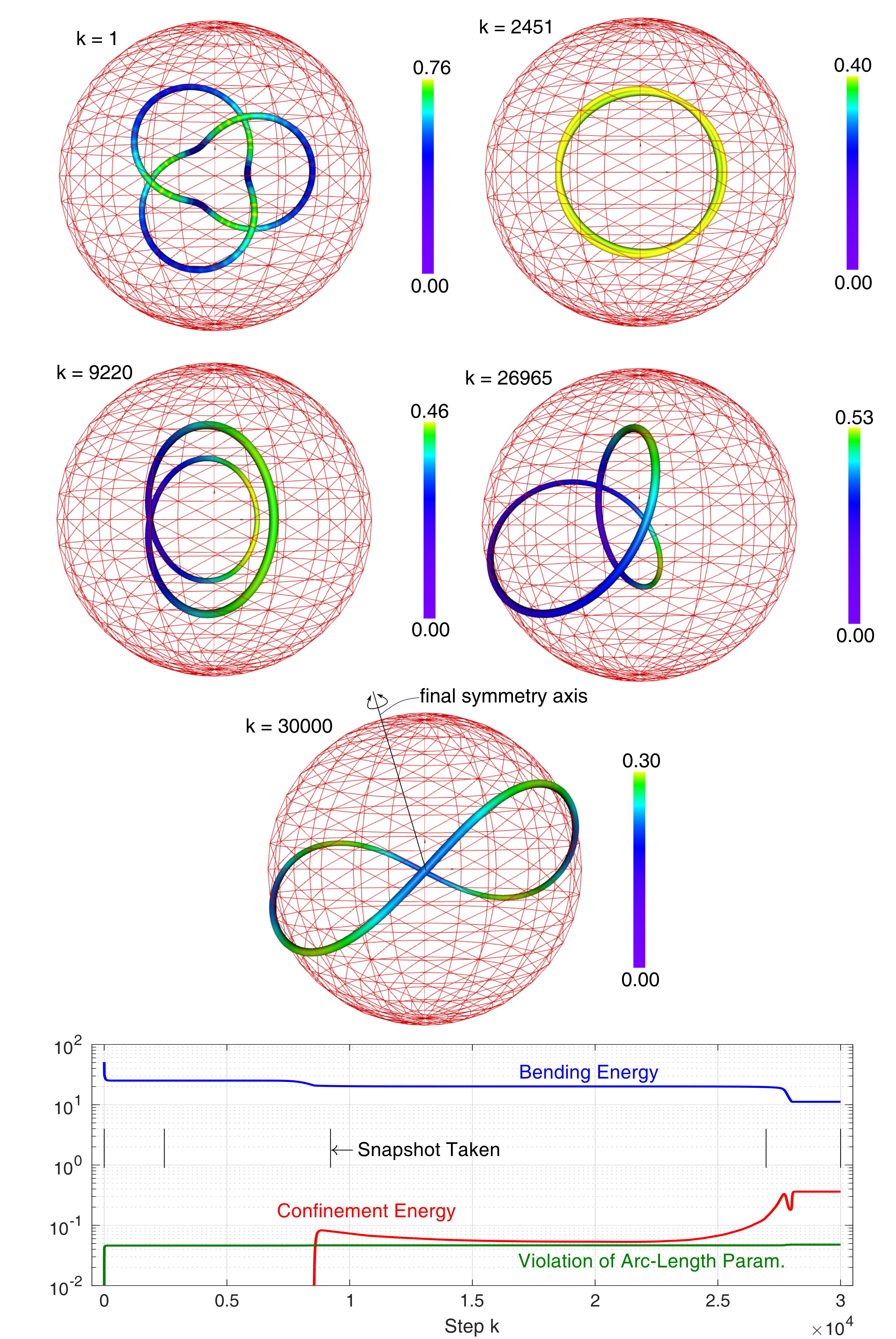
Figure 1. Evolution of a closed elastic curve in a ball of radius $R=4.6$ to a 1-2-clew. The number $k$ indicates the time steps, the color scheme represents local curvature. Confinement and total energy, and violation of arc-length parametrization are shown in the lower right panel.

When confining a rod of length $L$ to balls of varying radii, a multitude of equilibrium configurations is observed. Examples are illustrated in Figure 2 where we used $C_{4}$ and $C_{5}$ symmetric initial configurations. Both, the symmetry number $\nu$ and the winding number $\mu$ depend on the symmetry of the initial configuration and on the ratio $L/R$. All elasticae run close to the ball’s surface and slightly exceed the confining domain. With decreasing radius, either the winding number or the symmetry number are gradually increased by 2. This follows from an increasing number of self-intersections of the rod that always affect two of its segments. The gradient flow used to minimize the energy preserves certain symmetries. When starting with an even symmetry, the elastica is an odd-even-clew or an odd-circle as illustrated in Figure 2. An initially odd rotational symmetry in turn generally leads to even-odd-clews or even-circles. An exception is the transition from the 2-1-clew to the 1-2-clew as illustrated in the introductory example. This transition involves large deformations. When the radius of the ball is too small, the confinement is too restrictive for the curve to undergo such large transitions.

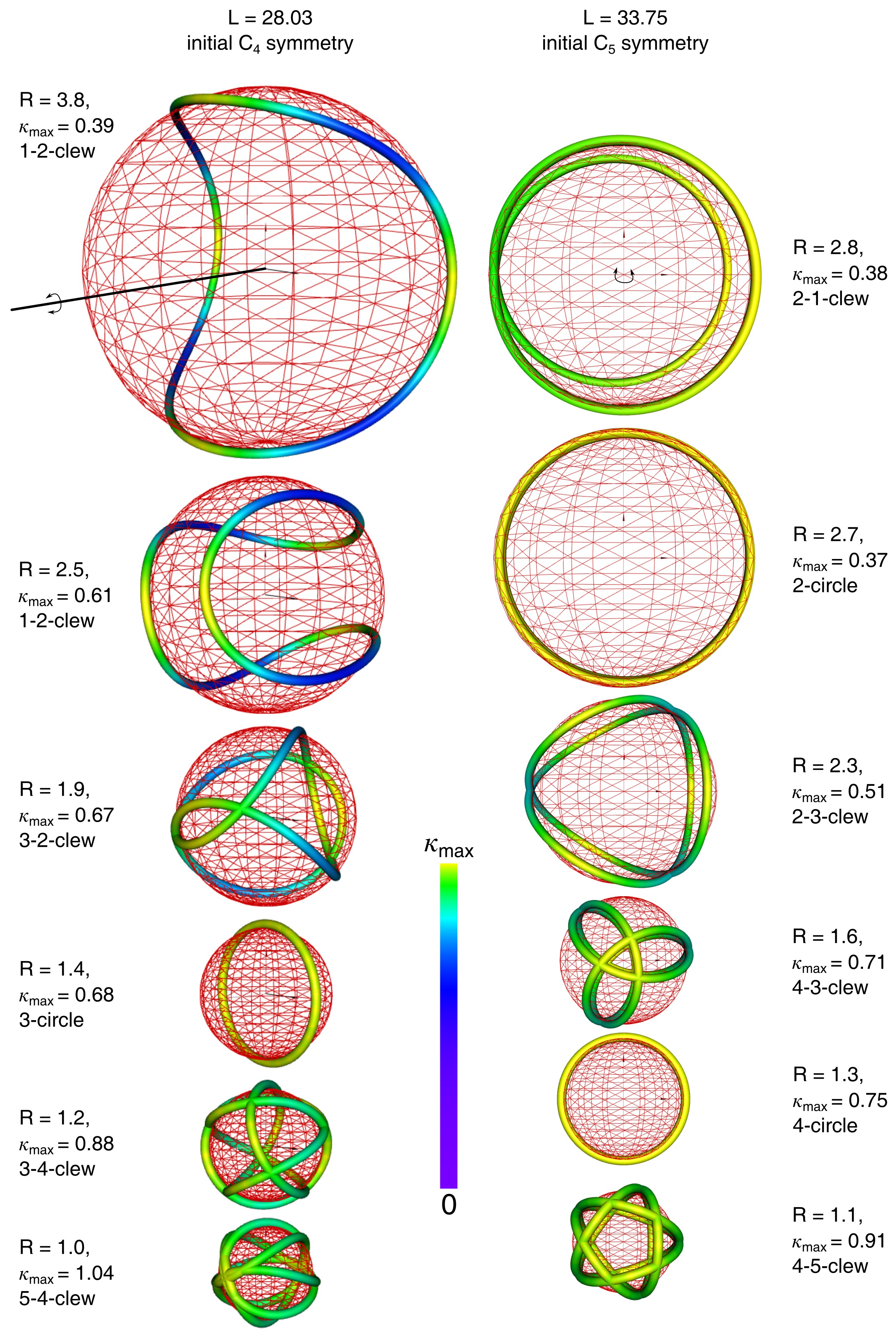
Figure 2. Elastica shapes obtained for two different initial configurations (left and right column, respectively) and varying radii $R$. The color of the rod indicates the local curvature. The symmetry axis of the left column is indicated for the top configuration. In the right column, symmetry and view axes coincide.

The unconfined elastica of a closed rod of length $L$ is the circle of radius $r_{L}=L/(2\pi)$. The bending energy of this elastica is given by $E_{L}=\kappa L/(2r_{L}^{2})=2\kappa\pi^{2}/L$. To categorize the equilibrium configurations of closed rods that are confined to balls of radius $R$, we evaluate $(E_{\text{bend}}/E_{L})^{1/2}$ as a function of $r_{L}/R$. The first quantity measures the excess bending induced by the confinement, whereas the second quantity determines how many times too small the confining ball is compared to the unconfined elastica. We remark that for $\mu$-fold covered circles, both quantities equal $\mu$.

When starting with the four- and five-fold symmetric initial configurations, we observe two distinct families of the bending energy dependency on the ratio $r_{L}/R$. The result is shown in Figure 3. The elasticae in the five-fold symmetric case follow the pattern 1-circle, 1-2-clew, 3-2-clew, 3-circle, 3-4-clew, 5-4-clew, etc. for increasing $r_{L}/R$. In the four-fold symmetric case, we find (1-circle, 1-2-clew,) 2-1-clew, 2-circle, 2-3-clew, 4-3-clew, 4-circle, 4-5-clew, and so on. The first two are special as they involve a large deformation of the rod when transiting from the even-odd to odd-even. Both patterns are very regular and are expected to continue for larger $r_{L}/R$.

During the unfolding process, intermediate nearly stationary configurations are observed. These include a shape that could be called a 1-3-clew or multiply covered circles that are completely inside the ball. This can be seen in Figure 1: The initial rod evolves into a two-fold covered circle in the first place; later, the circle opens up. These configurations seem to be saddle-point structures as they are attractive with respect to the previous configuration, whereas there are adjacent configurations with smaller total energy. As the numerical representation of the rod cannot match those saddle-points perfectly, the rod exits those configurations after a certain number of steps.

For irregularly shaped initial rod configurations, the previously described elastica shapes are found as well.  Hence, the symmetry of the final shape can be attributed to solely the ratio $r_{L}/R$ and to the question whether the initial configuration prefers the odd-even or even-odd elasticae family.

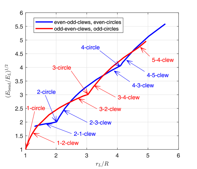
Figure 3. Normalized square root of the bending energy depending on the ratio $r_{L}/R$ for the two observed elastica families

Conjecture 3.2.

Consider a rod of length $L$ confined to a ball of radius $R$. Let $r_{L}=L/(2\pi)$ be the radius of the unconfined elastica and let $j\in\mathbf{N}$ be a positive integer with $j<r_{L}/R<j+1$. Then there is a number $\xi(j)\in(0,1)$ such that the globally least bent confined elastica is a $j$-($j+1$)-clew if $r_{L}/R<j+\xi$. Else, the global optimizer is the ($j+1$)-$j$-clew. If $r_{L}/R<1$, the flat 1-circle is an exactly confined elastica. In the cases where $r_{L}/R=j$ holds, the $j$-fold covered circle is the global elastica.

The parameter $\varepsilon$ can be understood as a length-scale of maximal penetration into the complement of $D$. The numerical results shown in Figure 4, indicate that

$$\max\limits_{j=0,\ldots,N}(|u_{h}^{k}(x_{j})|_{D}-1)_{+}=\mathcal{O}(\varepsilon).$$

Thus, the maximal penetration decreases linearly with $\varepsilon$ whilst not depending on whether the initial rod configuration lies inside $D$. This indicates that the estimate as sketched in Remark 2.5 is valid in the case of spherical confinements.

It can be observed that when varying $\varepsilon$ for the same initial configuration the final shape is not unique (cf. Figure 4): In the first example (dots in Figure 4), mainly 1-2-clews were obtained as final shapes, but for one value of $\varepsilon$, also a 2-1-clew could be observed. The second example that relaxed to a 2-3-clew for sufficiently small $\varepsilon$ (crosses in Figure 4), turned into a two-fold covered circle if the confinement was too weak.

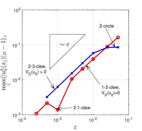
Figure 4. Maximal nodal penetration outside the confinement domain depending on $\varepsilon$.

Interestingly, all elasticae for $r_{L}/R\geq 1$ lie on the surface of the ball up to the penetration due to the finite potential. Brunnett and Crouch [16] derived a differential equation for the geodesic curvature $\kappa_{g}$ of the rod on the sphere, i.e. the projection of the total curvature on the tangent plane in each point:

$$\kappa_{g}^{\prime\prime}+\frac{1}{2}\kappa_{g}^{3}+C\kappa_{g}=0.$$

Here, $C$ is a constant consisting of the tension energy of the rod and the sphere square curvature. This differential equation can be solved by the Jacobi elliptic cosine function. The parameters of these functions must be adjusted such that the curvature is periodic. When using the solution to calculate the actual rod position, a nine-component ODE is solved, again imposing periodicitiy. This raises the question whether the resulting configurations coincide with our experimentally observed $\mu$-$\nu$-clews and $\mu$-circles, thus leading to an analytic definition of our clews. For the $\mu$-$\nu$-clew, $\nu$ and $\mu$ should arise when taking the periodic boundary conditions into account for the geodesic curvature and the rod position, respectively. It would be also of analytic interest if all elasticae confined to balls are actually elasticae on the sphere. A proof would however go beyond the scope of this manuscript.

We close our discussion by experimentally investigating closed curves confined to cylinders of different heights and radii.  As shown in Figure 5, large cylinder heights apparently lead to flat configurations that resemble semi-circles connected by straight lines. If the cylinder is long enough, we assume that the true global elastica consists of two semi-circles connected by two straight lines. If height and diameter are equal, we observe a shape similar to a 4-3-clew (for height and diameter 6) or a 3-2-clew (for height and diameter 8). Other combinations of height and diameter reveal a large variety of optimal shapes. A concise classification as in the case of spherical confinement however is not obvious.

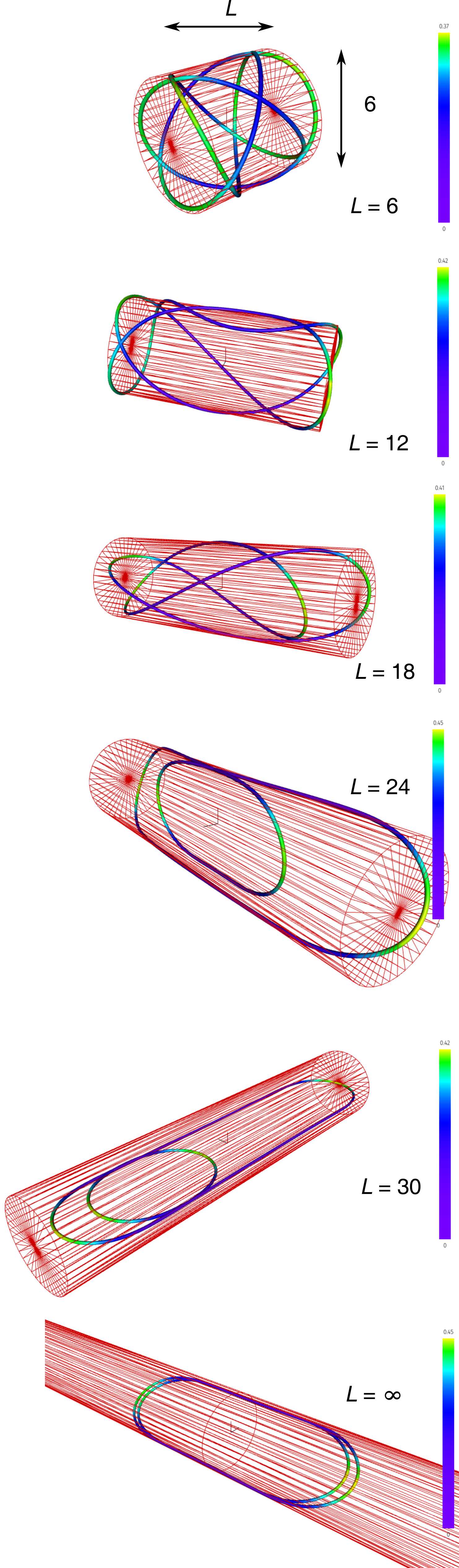
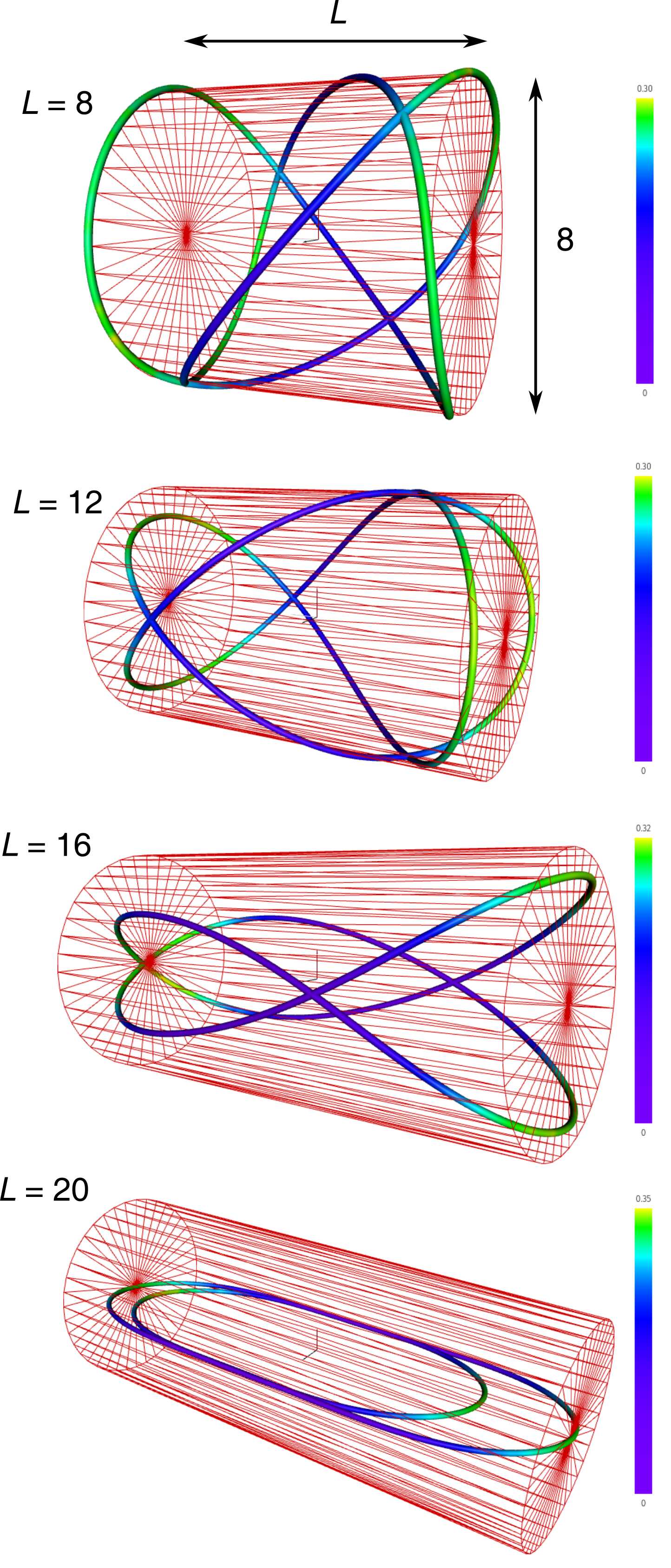
Figure 5. Stationary closed curves in cylindrical domains with radii $R=3$ (left) and $R=4$ (right) and different heights (increasing from top to bottom).

References

R

pages1 Rpages34 Rpages39 Rpages57 Rpages32 Rpages30 Rpages11 Rpages53 Rpages37 Rpages28 Rpages23 Rpages-1 Rpages1 Rpages18 Rpages3 Rpages14 Rpages27 Rpages94 Rpages23 Rpages1 Rpages22 Rpages-1 Rpages18 Rpages21 Rpages40 Rpages14 Rpages21 Rpages-1 Rpages29 Rpages14 Rpages9 Rpages-1 Rpages15 Rpages19 Rpages20 Rpages1 Rpages24 Rpages46 Rpages15 Rpages24 Rpages33

References

- [1] Alexander Balaeff, L. Mahadevan and Klaus Schulten “Modeling DNA loops using the theory of elasticity” In Phys. Rev. E 73 American Physical Society, 2006, pp. 031919 DOI: 10.1103/PhysRevE.73.031919
- [2] John W. Barrett, Harald Garcke and Robert Nürnberg “Finite element methods for fourth order axisymmetric geometric evolution equations” In J. Comput. Phys. 376, 2019, pp. 733–766 DOI: 10.1016/j.jcp.2018.10.006
- [3] John W. Barrett, Harald Garcke and Robert Nürnberg “Numerical approximation of anisotropic geometric evolution equations in the plane” In IMA J. Numer. Anal. 28.2, 2008, pp. 292–330 DOI: 10.1093/imanum/drm013
- [4] John W. Barrett, Harald Garcke and Robert Nürnberg “Numerical approximation of gradient flows for closed curves in ” In IMA J. Numer. Anal. 30.1, 2010, pp. 4–60 DOI: 10.1093/imanum/drp005
- [5] John W. Barrett, Harald Garcke and Robert Nürnberg “Stable discretizations of elastic flow in Riemannian manifolds” In SIAM J. Numer. Anal. 57.4, 2019, pp. 1987–2018 DOI: 10.1137/18M1227111
- [6] John W. Barrett, Harald Garcke and Robert Nürnberg “The approximation of planar curve evolutions by stable fully implicit finite element schemes that equidistribute” In Numer. Methods Partial Differential Equations 27.1, 2011, pp. 1–30 DOI: 10.1002/num.20637
- [7] Sören Bartels “A simple scheme for the approximation of the elastic flow of inextensible curves” In IMA J. Numer. Anal. 33.4, 2013, pp. 1115–1125 DOI: 10.1093/imanum/drs041
- [8] Sören Bartels “Finite element simulation of nonlinear bending models for thin elastic rods and plates” In Geometric partial differential equations. Part I 21, Handb. Numer. Anal. Elsevier/North-Holland, Amsterdam, 2020, pp. 221–273
- [9] Sören Bartels, Philipp Falk and Pascal Weyer “Knotevolve – a tool for relaxing knots and inextensible curves” https://aam.uni-freiburg.de/knotevolve/, 2020
- [10] Sören Bartels and Christian Palus “Stable gradient flow discretizations for simulating bilayer plate bending with isometry and obstacle constraints” drab050 In IMA Journal of Numerical Analysis, 2021 DOI: 10.1093/imanum/drab050
- [11] Sören Bartels and Philipp Reiter “Numerical solution of a bending-torsion model for elastic rods” In Numer. Math. 146.4, 2020, pp. 661–697 DOI: 10.1007/s00211-020-01156-6
- [12] Sören Bartels and Philipp Reiter “Stability of a simple scheme for the approximation of elastic knots and self-avoiding inextensible curves” In Math. Comp. 90.330, 2021, pp. 1499–1526 DOI: 10.1090/mcom/3633
- [13] Sören Bartels, Philipp Reiter and Johannes Riege “A simple scheme for the approximation of self-avoiding inextensible curves” In IMA J. Numer. Anal. 38.2, 2018, pp. 543–565 DOI: 10.1093/imanum/drx021
- [14] Andrea Bonito, Diane Guignard, Ricardo H. Nochetto and Shuo Yang “LDG approximation of large deformations of prestrained plates” In J. Comput. Phys. 448, 2022, pp. Paper No. 110719\bibrangessep27 DOI: 10.1016/j.jcp.2021.110719
- [15] L. Boué et al. “Spiral Patterns in the Packing of Flexible Structures” In Phys. Rev. Lett. 97 American Physical Society, 2006, pp. 166104 DOI: 10.1103/PhysRevLett.97.166104
- [16] Guido Brunnett and Peter E. Crouch “Elastic curves on the sphere” In Adv. Comput. Math. 2.1, 1994, pp. 23–40 DOI: 10.1007/BF02519034
- [17] M.. Choi et al. “Direct Observation of Biaxial Confinement of a Semiflexible Filament in a Channel” In Macromolecules 38.23, 2005, pp. 9882–9884 DOI: 10.1021/ma051348n
- [18] Anna Dall’Acqua, Chun-Chi Lin and Paola Pozzi “Evolution of open elastic curves in subject to fixed length and natural boundary conditions” In Analysis (Berlin) 34.2, 2014, pp. 209–222 DOI: 10.1515/anly-2014-1249
- [19] Klaus Deckelnick and Gerhard Dziuk “Error analysis for the elastic flow of parametrized curves” In Math. Comp. 78.266, 2009, pp. 645–671 DOI: 10.1090/S0025-5718-08-02176-5
- [20] Klaus Deckelnick, Gerhard Dziuk and Charles M. Elliott “Computation of geometric partial differential equations and mean curvature flow” In Acta Numer. 14, 2005, pp. 139–232 DOI: 10.1017/S0962492904000224
- [21] Ellis Harold Dill “Kirchhoff’s theory of rods” In Arch. Hist. Exact Sci. 44.1, 1992, pp. 1–23 DOI: 10.1007/BF00379680
- [22] C.. Donato, M… Gomes and R.. Souza “Scaling properties in the packing of crumpled wires” In Phys. Rev. E 67 American Physical Society, 2003, pp. 026110 DOI: 10.1103/PhysRevE.67.026110
- [23] Patrick W. Dondl, Luca Mugnai and Matthias Röger “Confined elastic curves” In SIAM J. Appl. Math. 71.6, 2011, pp. 2205–2226 DOI: 10.1137/100805339
- [24] Willy Dörfler and Robert Nürnberg “Discrete gradient flows for general curvature energies” In SIAM J. Sci. Comput. 41.3, 2019, pp. A2012–A2036 DOI: 10.1137/18M122844X
- [25] Gerhard Dziuk, Ernst Kuwert and Reiner Schätzle “Evolution of elastic curves in : existence and computation” In SIAM J. Math. Anal. 33.5, 2002, pp. 1228–1245 DOI: 10.1137/S0036141001383709
- [26] Patrick B. Furrer, Robert S. Manning and John H. Maddocks “DNA Rings with Multiple Energy Minima” In Biophysical Journal 79.1, 2000, pp. 116–136 DOI: https://doi.org/10.1016/S0006-3495(00)76277-1
- [27] Henryk Gerlach and Heiko Mosel “What are the longest ropes on the unit sphere?” In Arch. Ration. Mech. Anal. 201.1, 2011, pp. 303–342 DOI: 10.1007/s00205-010-0390-y
- [28] A.. Green, N. Laws and P.. Naghdi “A linear theory of straight elastic rods” In Arch. Rational Mech. Anal. 25.4, 1967, pp. 285–298 DOI: 10.1007/BF00250931
- [29] Martin Grothaus and Nicole Marheineke “On a nonlinear partial differential algebraic system arising in the technical textile industry: analysis and numerics” In IMA J. Numer. Anal. 36.4, 2016, pp. 1783–1803 DOI: 10.1093/imanum/drv056
- [30] Peter Hornung “Deformation of framed curves with boundary conditions” In Calc. Var. Partial Differential Equations 60.3, 2021, pp. Paper No. 87\bibrangessep26 DOI: 10.1007/s00526-021-01980-0
- [31] G. Kirchhoff “Ueber das Gleichgewicht und die Bewegung eines unendlich dünnen elastischen Stabes” In J. Reine Angew. Math. 56, 1859, pp. 285–313 DOI: 10.1515/crll.1859.56.285
- [32] Joel Langer and David A. Singer “Curve straightening and a minimax argument for closed elastic curves” In Topology 24.1, 1985, pp. 75–88 DOI: 10.1016/0040-9383(85)90046-1
- [33] Joel Langer and David A. Singer “Knotted elastic curves in ” In J. London Math. Soc. (2) 30.3, 1984, pp. 512–520 DOI: 10.1112/jlms/s2-30.3.512
- [34] Giovanni Leoni “A first course in Sobolev spaces” 181, Graduate Studies in Mathematics American Mathematical Society, Providence, RI, 2017, pp. xxii+734 DOI: 10.1090/gsm/181
- [35] Angelika Manhart, Dietmar Oelz, Christian Schmeiser and Nikolaos Sfakianakis “An extended filament based lamellipodium model produces various moving cell shapes in the presence of chemotactic signals” In J. Theoret. Biol. 382, 2015, pp. 244–258 DOI: 10.1016/j.jtbi.2015.06.044
- [36] Maria Giovanna Mora and Stefan Müller “Derivation of the nonlinear bending-torsion theory for inextensible rods by -convergence” In Calc. Var. Partial Differential Equations 18.3, 2003, pp. 287–305 DOI: 10.1007/s00526-003-0204-2
- [37] Connor G. Mulcahy, Tianxiang Su, Nathan Wicks and Pedro M. Reis “Extending the Reach of a Rod Injected Into a Cylinder Through Axial Rotation” 051003 In Journal of Applied Mechanics 83.5, 2016 DOI: 10.1115/1.4032500
- [38] D.. Öelz “On the curve straightening flow of inextensible, open, planar curves” In SeMA J., 2011, pp. 5–24 DOI: 10.1007/bf03322585
- [39] Katja Ostermeir, Karen Alim and Erwin Frey “Buckling of stiff polymer rings in weak spherical confinement” In Phys. Rev. E 81 American Physical Society, 2010, pp. 061802 DOI: 10.1103/PhysRevE.81.061802
- [40] Thomas Ranner “A stable finite element method for low inertia undulatory locomotion in three dimensions” In Appl. Numer. Math. 156, 2020, pp. 422–445 DOI: 10.1016/j.apnum.2020.05.009
- [41] Philipp Reiter and Henrik Schumacher “Sobolev gradients for the Möbius energy” In Arch. Ration. Mech. Anal. 242.2, 2021, pp. 701–746 DOI: 10.1007/s00205-021-01680-1
- [42] Yaoming Shi and John E. Hearst “The Kirchhoff elastic rod, the nonlinear Schrödinger equation, and DNA supercoiling” In The Journal of Chemical Physics 101.6, 1994, pp. 5186–5200 DOI: 10.1063/1.468506
- [43] Shawn Walker “A Descent Scheme for Thick Elastic Curves with Self-contact and Container Constraints” In Preprint, 2021 URL: https://www.math.lsu.edu/~walker/pdfs/Walker2021_elastic_curve_self_contact.pdf
- [44] Shawn W. Walker “Shape optimization of self-avoiding curves” In J. Comput. Phys. 311, 2016, pp. 275–298 DOI: 10.1016/j.jcp.2016.02.011
- [45] Stephan Wojtowytsch “Confined elasticae and the buckling of cylindrical shells” In Adv. Calc. Var. 14.4, 2021, pp. 555–587 DOI: 10.1515/acv-2019-0033