An inverse problem for a semi-linear wave equation: a numerical study

Abstract

We consider an inverse problem of recovering a potential associated to a semi-linear wave equation with a quadratic nonlinearity in $1+1$ dimensions. We develop a numerical scheme to determine the potential from a noisy Dirichlet-to-Neumann map on the lateral boundary. The scheme is based on the recent higher order linearization method [20]. We also present an approach to numerically estimating two-dimensional derivatives of noisy data via Tikhonov regularization. The methods are tested using synthetic noisy measurements of the Dirichlet-to-Neumann map. Various examples of reconstructions of the potential functions are given.

This paper is a continuation of [20] into a computational direction. We study an inverse boundary value problem for the one-dimensional non-linear wave equation

$$\begin{cases}\frac{\partial^{2}}{\partial t^{2}}u(x,t)=\frac{\partial}{\partial x^{2}}u(x,t)-q(x,t)\hskip 0.5ptu(x,t)^{2}&(x,t)\in[a,b]\times[0,T],\\ u(a,t)=f^{L}(t),&t\in[0,T],\\ u(b,t)=f^{R}(t),&t\in[0,T],\\ u(x,0)=\partial_{t}u(x,0)=0&x\in[a,b].\end{cases}$$ (1)

It was shown in [20] that there exists a unique small solution to (1) if $f^{L},f^{R}\in H^{s}([0,T])$ have small enough norms in $H^{s}([0,T])$ for sufficiently large $s>0$. Let us denote the lateral boundary of $[a,b]\times[0,T]$ by

$$\Sigma:=\{a,b\}\times[0,T].$$

The Sobolev space $H^{s+1}(\Sigma)$ is naturally isomorphic to $H^{s+1}([0,T])\times H^{s+1}([0,T])$. The Dirichlet-to-Neumann map (DN map) $\Lambda_{q}$ is then defined as

$$\Lambda_{q} :H^{s+1}([0,T])\times H^{s+1}([0,T])\to H^{s}(\Sigma),$$

$$\quad\{f^{L},f^{R}\}\mapsto\partial_{\nu}u\big{|}_{\Sigma},$$

where $u$ solves (1) and $\nu$ is the outward pointing normal of $\Sigma$. The notations $f^{L}$ and $f^{R}$ refer to the boundary value on the left and right side of $\Sigma$ as in (1). The inverse problem we consider in this paper is the recovery of the unknown potential function $q\in C^{\infty}([a,b]\times[0,T])$ from the DN map $\Lambda_{q}$. It was shown in [20] that the DN map uniquely determines the unknown potential $q(x,t)$. The work also provided a stable reconstruction algorithm. In this work we implement the reconstruction algorithm numerically. To the best of our knowledge, this is the first work that provides numerical results based on using non-linearity as a beneficial tool for inverse problems of nonlinear wave equations.

Our numerical reconstruction algorithm follows the recent work [20]. The work is based on the recent higher order linearization method, which uses boundary values with several parameters (two in this paper) and obtains new linearized equations after differentiating with respect to these parameters. The reconstruction algorithm based on the method is fast and straightforward to implement. Given a suitable measurement data set, the inversion is done practically in real time. We explain the higher order linearization method and the the numerical reconstruction in Section 1. Our reconstruction works equally well for both time independent and time dependent potentials.

The idea of higher order linearizations was developed by Kurylev, Lassas and Uhlmann [16]. They observed that non-linearity can be used as a beneficial tool in inverse problems and recovered a Lorentzian manifold up to a conformal change from local measurements for the scalar wave equation with quadratic nonlinearity. The measurements in the work were modeled by a source-to-solution mapping, which assigns to a source the corresponding solution of the nonlinear wave equation restricted to the measurement set.

Instead of measurements modeled by source-to-solution mapping, the higher order linearization method evolved to a tool for inverse problems for boundary value problems in the context of elliptic equations in [8, 14, 15, 18, 19]. Especially the works [14, 15, 19] introduced the concept of measurement function (the term measurement function was coined in [20]) that allowed to apply the higher order linearization method also for inverse problems of boundary value problems for nonlinear wave equations. The works [11, 12, 21] study inverse problems for boundary value problems for nonlinear wave equations by using the aforementioned method. We refer the reader to the works [1, 4, 5, 6, 7, 17, 23, 24, 29, 30, 31] for more examples of inverse problems for nonlinear wave type and hyperbolic equations, and to [12] for additional references. The very recent work [28] does a numerical study of an inverse problem for a nonlinear elliptic equation by using the higher order linearization method.

In the current paper, we use the higher order linearization method to measure the response coming from nonlinear interactions of waves that approximate delta functions. This means that for each $(x_{0},t_{0})\in[a,b]\times[0,T]$, where we wish to recover the unknown potential $q$, we need to make one measurement. One can think that a possible downside of this approach is that since it relies in this sense point-wise measurements, it does not average out well the noise in the measurements. However, as we will observe, our reconstruction is good even in the presence of a reasonable noise. We will discuss this matter in Section 4.

The structure of this paper is as follows. In Section 1 we first discuss the theoretical results of [20]. After that we discuss how the theoretical results are translated into a numerical recovery method. Section 2 concerns the numerical implementation of solving the forward problem (1). The forward problem is solved by a simple finite difference method and it is needed to build the synthetic DN map. We present an example and discuss the convergence of the finite difference method. In Section 3 we discuss an approach for approximating two dimensional derivatives by using a regularization method. In Section 4 we discuss a numerical implementation of the reconstruction algorithm for the recovery of the potential $q$ from the associated DN map. Finally, in Section 5 we present and discuss examples of recoveries of various potentials.

1 Preliminaries

1.1 The higher order linearization method

Here we explain how to recover $q(x,t)$ theoretically from the DN map $\Lambda_{q}$ associated with (1). As mentioned, a theoretical method for recovering $q$ was established in the authors’ earlier work [20], where stability of the recovery was also considered. The recovery in [20] was based on the higher order linearization method, which we now explain. We follow the notation of the work [20] and refer to the work for justifications and details of the following formal discussion.

Let $f_{1},\hskip 0.5ptf_{2}\in H^{s+1}(\Sigma)$, $s>1$. To avoid confusion with the notation, we recall that $f_{1}=(f_{1}^{L},f_{1}^{R})$ and $f_{2}=(f_{2}^{L},f_{2}^{R})$, where each component function belongs to $H^{s+1}([0,T])$. Let us consider the family $u_{\varepsilon_{1}f_{1}+\varepsilon_{2}f_{2}}$ of solutions to

$$\begin{cases}\square u_{\varepsilon_{1}f_{1}+\varepsilon_{2}f_{2}}(x,t)=-q(x,t)\hskip 0.5ptu_{\varepsilon_{1}f_{1}+\varepsilon_{2}f_{2}}^{2}(x,t),&(x,t)\in[a,b]\times[0,T],\\ u_{\varepsilon_{1}f_{1}+\varepsilon_{2}f_{2}}(x,t)=\varepsilon_{1}f_{1}(x,t)+\varepsilon_{2}f_{2}(x,t),&(x,t)\in\Sigma,\\ u_{\varepsilon_{1}f_{1}+\varepsilon_{2}f_{2}}(x,0)=\partial_{t}u_{\varepsilon_{1}f_{1}+\varepsilon_{2}f_{2}}(x,0)=0,&x\in[a,b],\end{cases}$$ (2)

parametrized by small parameters $\varepsilon_{1},\varepsilon_{2}\in\mathbb{R}$. Here we have denoted

$$\square:=\frac{\partial^{2}}{\partial t^{2}}-\frac{\partial}{\partial x^{2}}.$$

We differentiate the equation (2) with respect to the parameters $\varepsilon_{1}$ and $\varepsilon_{2}$. A formal calculation (justified in [20]) shows that the mixed derivative

$$w:=\frac{\partial}{\partial\varepsilon_{1}}\frac{\partial}{\partial\varepsilon_{2}}\Big{|}_{\varepsilon_{1}=\varepsilon_{2}=0}u_{\varepsilon_{1}f_{1}+\varepsilon_{2}f_{2}}$$ (3)

is a function whose initial and boundary data vanish and that satisfies

$$\frac{\partial^{2}}{\partial t^{2}}w(x,t)=\frac{\partial}{\partial x^{2}}w(x,t)-2q(x,t)v_{1}(x,t)v_{2}(x,t).$$ (4)

The functions $v_{j}$ in (4), for $j=1,2$, solve the linear wave equation

$$\begin{cases}\frac{\partial^{2}}{\partial t^{2}}v_{j}(x,t)=\frac{\partial}{\partial x^{2}}v_{j}(x,t),&(x,t)\in[a,b]\times[0,T],\\ v_{j}(x,t)=f_{j}(x,t),&(x,t)\in\Sigma,\\ v_{j}(x,0)=\partial v_{j}(x,0)=0,&x\in[a,b].\end{cases}$$ (5)

This way we have produced new linear equations from the non-linear equation (1). Note that the equation for $v_{j}$ is independent of the unknown potential $q(x,t)$. The function $w$ defined by (3) is called the second linearization of $u_{\varepsilon_{1}f_{1}+\varepsilon_{2}f_{2}}$.

If the DN map is known, then the normal derivative $\partial_{\nu}w$ on the lateral boundary $\Sigma$ of the second linearization is also known, because

$$\partial_{\nu}w=\partial_{\nu}\left(\partial^{2}_{\varepsilon_{1}\varepsilon_{2}}|_{\varepsilon_{1}=\varepsilon_{2}=0}\hskip 0.5ptu_{\varepsilon_{1}f_{1}+\varepsilon_{2}f_{2}}\right)=\partial^{2}_{\varepsilon_{1}\varepsilon_{2}}|_{\varepsilon_{1}=\varepsilon_{2}=0}\hskip 0.5pt\Lambda_{q}(\varepsilon_{1}f_{1}+\varepsilon_{2}f_{2}).$$

(See [20] for justification of this calculation.) We let $v_{0}$ be an auxiliary function solving $\square v_{0}=0$ in $[a,b]\times[0,T]$ with $v_{0}(x,T)=\partial_{t}v_{0}(x,T)=0$ for $x\in[a,b]$. The function $v_{0}$ is called the measurement function. The function $v_{0}$ is used to compensate the fact that $\partial_{\nu}w$ is not known on $\{t=T\}$ from the DN map $H^{s+1}(\Sigma)\to H^{s}(\Sigma)$. By multiplying (4) by $v_{0}$ and integrating by parts on $[a,b]\times[0,T]$, we arrive at the integral identity

$$\begin{split}\int_{\Sigma}v_{0}\hskip 0.5pt\partial^{2}_{\varepsilon_{1}\varepsilon_{2}}|_{\varepsilon_{1}=\varepsilon_{2}=0}\Lambda_{q}(\varepsilon_{1}f_{1}+\varepsilon_{2}f_{2})\hskip 0.5pt\mathrm{d}\Sigma&=\int_{[a,b]\times[0,T]}\hskip 0.5ptv_{0}\hskip 0.5pt\square w\hskip 0.5pt\mathrm{d}x\hskip 0.5pt\mathrm{d}t\\ &=-2\int_{[a,b]\times[0,T]}q\hskip 0.5ptv_{0}\hskip 0.5ptv_{1}\hskip 0.5ptv_{2}\hskip 0.5pt\mathrm{d}x\hskip 0.5pt\mathrm{d}t.\end{split}$$ (6)

Thus the quantity

$$\int_{[a,b]\times[0,T]}q\hskip 0.5ptv_{0}\hskip 0.5ptv_{1}\hskip 0.5ptv_{2}\hskip 0.5pt\mathrm{d}x\hskip 0.5pt\mathrm{d}t$$ (7)

is known from the knowledge of the DN map. The integral identity (6) holds for arbitrary solutions $v_{0},v_{1}$ and $v_{2}$ to $\square v=0$ in $[a,b]\times[0,T]$ satisfying the initial conditions $v_{0}(x,T)=\partial_{t}v_{0}(x,T)=0$ and $v_{k}(x,0)=\partial_{t}v_{k}(x,0)=0$ for $k=1,2$ and $x\in[a,b]$.

To recover information about $q$ from (7), we need to make an appropriate choice of the functions $v_{1}$ and $v_{2}$. Let $\chi\in C_{c}^{\infty}(\mathbb{R})$ be a cut-off function supported close to $0\in\mathbb{R}$ with $\chi(0)=1$. For $\tau>0$, we let $H^{\tau}\in C_{c}^{\infty}(\mathbb{R})$ be a function defined by

$$H^{\tau}(\hskip 0.5ptl\hskip 0.5pt)=\chi(\hskip 0.5ptl\hskip 0.5pt)\tau^{1/2}\mathrm{e}^{-\frac{1}{2}\tau\,l^{2}},\quad l\in\mathbb{R}.$$

Let $(x_{0},t_{0})\in[a,b]\times[0,T]$ and define a family of functions by

$$\begin{split}H_{1}^{\tau}(x,t)&:=H^{\tau}\big{(}(x-x_{0})-(t-t_{0})\big{)},\\ H_{2}^{\tau}(x,t)&:=H^{\tau}\big{(}(x-x_{0})+(t-t_{0})\big{)}\end{split}$$ (8)

parametrized by $\tau$. Note that the functions $H^{\tau}_{k}(x,t)=0$, $k=1,2$, solve the wave equation and they are supported outside neighborhoods of $\{t=0\}$ and $\{t=T\}$ if the support of $\chi$ is chosen small enough. For $\tau>0$, we then set

$$\begin{cases}v_{1}=H_{1}^{\tau},&\ f_{1}=\big{(}H_{1}^{\tau}(a,t),H_{1}^{\tau}(b,t)\big{)}\\ v_{2}=H_{2}^{\tau},&\ f_{2}=\big{(}H_{2}^{\tau}(a,t),H_{2}^{\tau}(b,t)\big{)}\end{cases}$$ (9)

Here we suppressed the $\tau$ dependence of $v_{1}$ and $v_{2}$ in the notation. As the function $v_{0}$ we take $H_{1}^{\tau}$ at fixed $\tau=1$:

$$v_{0}=H_{1}^{\tau}|_{\tau=1},\quad\psi=v_{0}|_{\Sigma}.$$ (10)

Next we observe that the product of $v_{1}=H_{1}^{\tau}$ and $v_{2}=H_{2}^{\tau}$ approximates the delta distribution at $(x_{0},t_{0})$, when $\tau$ is large. Indeed, by [20, Lemma 3] we have that

$$q(x_{0},t_{0})-\frac{1}{\pi}\int_{[a,b]\times[0,T]}q(x,t)H_{1}^{\tau}(x,t)H_{2}^{\tau}(x,t)dxdt=\mathcal{O}(\tau^{-1/2}).$$ (11)

It was also proved in [20] that the implicit constant on the right hand side of (11) is independent of the chosen point $(x_{0},t_{0})$. In particular $\frac{1}{\pi}H_{1}^{\tau}H_{2}^{\tau}$ converges to the delta distribution at $(x_{0},t_{0})$ in the sense of distributions, as $\tau\to\infty$. It follows by taking $\tau\to\infty$ in (6) that

$$-2\pi q(x_{0},t_{0})=\lim_{\tau\to\infty}\int_{\Sigma}\psi\hskip 0.5pt\partial^{2}_{\varepsilon_{1}\varepsilon_{2}}|_{\varepsilon_{1}=\varepsilon_{2}=0}\Lambda_{q}(\varepsilon_{1}f_{1}+\varepsilon_{2}f_{2})\hskip 0.5pt\mathrm{d}\Sigma.$$ (12)

Since the right hand side of this equation is given by the DN map of (1), we have recovered $q(x_{0},t_{0})$. Since $(x_{0},t_{0})$ in the above argument was arbitrary, we may similarly recover $q$ at any point in the set pictured in Figure 1.

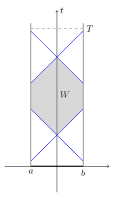
Figure 1: The set $W$, where we can recover the potential $q(x,t)$. In the 1+1 dimensional case this is the set, where we can make two approximate plane waves (one travelling to the left and the other to the right) collide.

This set is called the admissible set and denoted by $W$. It is a set that can be reached from both the left and right sides of the lateral boundary by sending waves and from which waves can propagate back to the lateral boundary $\Sigma$.

1.2 The numerical recovery method

Let us then explain how the theoretical recovery method described above transforms into a numerical recovery method. We conclude this section by explaining how we tested the quality of the numerical recovery method.

Our numerical recovery method is based on the identity (12), which entails choosing suitable boundary values, taking a limit in $\tau$ and calculating derivatives with respect to the $\varepsilon_{1}$ and $\varepsilon_{2}$ parameters. To evaluate the mixed derivative $\partial^{2}_{\varepsilon_{1}\varepsilon_{2}}|_{\varepsilon_{1}=\varepsilon_{2}=0}\Lambda_{q}(\varepsilon_{1}f_{1}+\varepsilon_{2}f_{2})$ in (12), we experimented with two approaches to evaluate this derivative:

(1) A finite difference approximation.

(2) An approach using regularization, where differentiation is regarded as an inverse operation to integration.

Let us first discuss the first approach (1). Finite differences were used in [20] to prove a Hölder stability estimate for the recovery of $q$. There the mixed derivatives $\partial^{2}_{\varepsilon_{1}\varepsilon_{2}}|_{\varepsilon_{1}=\varepsilon_{2}=0}\Lambda_{q}(\varepsilon_{1}f_{1}+\varepsilon_{2}f_{2})$ were replaced by the finite differences

$$D^{2}_{\epsilon_{1},\epsilon_{2}}\big{|}_{\varepsilon_{1}=\varepsilon_{2}=0}\Lambda_{q}(\varepsilon_{1}f_{1}+\varepsilon_{2}f_{2}):=\frac{1}{\epsilon_{1}\epsilon_{2}}\left(\Lambda_{q}(\varepsilon_{1}f_{1}+\varepsilon_{2}f_{2})-\Lambda_{q}(\varepsilon_{1}f_{1})-\Lambda_{q}(\varepsilon_{2}f_{2})\right).$$ (13)

For finite differences, the integral identity

$$-2\int_{[a,b]\times[0,T]}q\hskip 0.5ptv_{0}\hskip 0.5ptv_{1}\hskip 0.5ptv_{2}\hskip 0.5pt\mathrm{d}x\hskip 0.5pt\mathrm{d}t =\int_{\Sigma}v_{0}\hskip 0.5ptD_{\varepsilon_{1},\varepsilon_{2}}^{2}\Big{|}_{\varepsilon_{1}=\varepsilon_{2}=0}\Lambda_{q}(\varepsilon_{1}f_{1}+\varepsilon_{2}f_{2})\hskip 0.5pt\mathrm{d}S$$ (14)

$$\qquad\qquad\qquad\qquad+\frac{1}{\varepsilon_{1}\varepsilon_{2}}\int_{[a,b]\times[0,T]}v_{0}\square\hskip 0.5pt\widetilde{\mathcal{R}}\hskip 0.5pt\mathrm{d}x\hskip 0.5pt\mathrm{d}t$$

is the replacement of (6). This identity holds for any $f_{1},f_{2}\in H^{s}(\Sigma)$, $s\in\mathbb{N}$, and corresponding solutions $v_{1}$ and $v_{2}$ to (5). Here $\square\hskip 0.5pt\widetilde{\mathcal{R}}=\mathcal{O}(\langle\varepsilon_{1},\varepsilon_{2}\rangle^{3})$ in $H^{s+1}([a,b]\times[0,T])$, where $\langle\varepsilon_{1},\varepsilon_{2}\rangle^{3}$ denotes an unspecified homogeneous polynomial of order $3$ in $\varepsilon_{1}$ and $\varepsilon_{2}$. We refer to [20] for more details. Here we suffice to remark that the last integral in (14) is of the size $\max(\varepsilon_{1},\varepsilon_{2})$, which is small.

We choose $f_{1},f_{2}$ and $\psi$ as in (9)–(10). We also introduce noise $\mathcal{E}$ to our measurements. We assume that $\mathcal{E}$ is a bounded,

$$\lVert\mathcal{E}(f)\rVert_{H^{r}(\Sigma)}\leq\delta,$$ (15)

possibly non-linear, mapping $H^{s+1}(\Sigma)\to H^{r}(\Sigma)$, $r\in\mathbb{R}$ and $r\leq s$. In this case, for our choices for $f_{1}$ and $f_{2}$, the equation (14) is replaced by

$$-2\int_{[a,b]\times[0,T]}q\hskip 0.5ptv_{0}\hskip 0.5ptv_{1}\hskip 0.5ptv_{2}\hskip 0.5pt\mathrm{d}x\hskip 0.5pt\mathrm{d}t =\int_{\Sigma}\psi\hskip 0.5ptD_{\varepsilon_{1},\varepsilon_{2}}^{2}\Big{|}_{\varepsilon_{1}=\varepsilon_{2}=0}(\Lambda_{q}+\mathcal{E})(\varepsilon_{1}f_{1}+\varepsilon_{2}f_{2})\hskip 0.5pt\mathrm{d}\Sigma$$ (16)

$$\qquad+\frac{1}{\varepsilon_{1}\varepsilon_{2}}\int_{[a,b]\times[0,T]}v_{0}\square\hskip 0.5pt\widetilde{\mathcal{R}}\hskip 0.5pt\mathrm{d}x\hskip 0.5pt\mathrm{d}t.$$

It was shown in [20, Theorem 3] that there is a constant $C>0$ such that

$$\Big{|}-q(x_{0},t_{0})-\frac{1}{2\pi}\int_{\Sigma}\psi\,D_{\varepsilon_{1},\varepsilon_{2}}^{2}\Big{|}_{\varepsilon_{1}=\varepsilon_{2}=0}(\Lambda_{q}+\mathcal{E})(\varepsilon_{1}f_{1}+\varepsilon_{2}f_{2})\mathrm{d}\Sigma\Big{|}\leq C\delta^{\sigma(s)},$$ (17)

The exponent $\sigma(s)$ is $\frac{1}{6s+15}$. The estimate (17) is a Hölder stability estimate for the recovery of $q$. It is obtained by optimizing the right hand side of (16) with respect to the parameters $\varepsilon_{1},\varepsilon_{2}$ and $\tau$. If one computes the integral in (17) and if the noise is small, then the integral is approximatively the potential $q$ at the point $(x_{0},t_{0})$. This is the basis of our numerical reconstruction of $q$.

The optimal choice of $\varepsilon_{1},\varepsilon_{2}$ and $\tau$ depends on some constants, mainly on a priori assumptions on the potentials and the size of the noise. While the constants can in principle be calculated, we do not attempt to do that. Instead, we suffice to experiment by choosing small non-zero values for $\varepsilon_{1},\varepsilon_{2}>0$ and a large finite value for $\tau$. We will discuss our choices for $\varepsilon_{1}$ and $\varepsilon_{2}$ more carefully in Sections 3 and 4.1. The large parameter $\tau$ will be chosen by studying the size of the error term in (11). We observe experimentally that $\tau=700$ and $\max(\varepsilon_{1},\varepsilon_{2})\approx 0.01$ produces good results in the examples we consider in Section 5.

Let us then describe our second approach (2) for calculating the mixed derivative $\partial^{2}_{\varepsilon_{1}\varepsilon_{2}}|_{\varepsilon_{1}=\varepsilon_{2}=0}\Lambda_{q}(\varepsilon_{1}f_{1}+\varepsilon_{2}f_{2})$. For this, let us denote

$$F(s,t)=\Lambda_{q}(sf_{1}+tf_{2}).$$

By the fundamental theorem of calculus

$$\begin{split}\int_{\beta}^{\varepsilon_{1}}\int_{\alpha}^{\varepsilon_{2}}\partial_{s}\partial_{t}F(s,t)\mathrm{d}s\hskip 0.5pt\mathrm{d}t&=F(\varepsilon_{1},\varepsilon_{2})-F(\alpha,\varepsilon_{2})-F(\varepsilon_{1},\beta)+F(\alpha,\beta)\\ &\quad\text{ for all }\varepsilon_{1}\text{ and }\varepsilon_{2}\text{ small enough}.\end{split}$$ (18)

Since the identity above holds for all $\varepsilon_{1}$ and $\varepsilon_{2}$ small enough, we consider it as system of equations parametrized by $\varepsilon_{1}$ and $\varepsilon_{2}$. Assume now that there is some error or noise on the right hand side of the equations in (18). Fix also $\alpha$ and $\beta$. The approach (2) is based on the question if in this case we can find an approximation for $\partial_{s}\partial_{t}F(s,t)$ by solving the system (18)? The system is at least typically ill-posed, so in general the answer is no. However, one can choose a suitable regularization scheme depending on known properties of the measurement noise and the boundary data to solve the system approximately. We find an approximate solution $\partial_{s}\partial_{t}F(s,t)$ by using Tikhonov regularization. An approximation of $\partial^{2}_{\varepsilon_{1}\varepsilon_{2}}|_{\varepsilon_{1}=\varepsilon_{2}=0}\Lambda(\varepsilon_{1}f_{1}+\varepsilon_{2}f_{2})$ is then $F(0,0)$. This is the approach (2). We call the approximate solution obtained in this way the regularized mixed derivative.

We end this section by discussing how our reconstruction method is implemented. The reconstruction is non-iterative and splits into a few steps. In Section 5 we compare exact potentials $q$ to the approximative ones obtained by our reconstruction method. To demonstrate reconstruction of a potential function, we do the following steps:
a) Fix a grid for the domain $[a,b]\times[0,T]$ and a point $(x_{0},t_{0})$ of the grid. We aim to recover $q(x_{0},t_{0})$. Corresponding to $(x_{0},t_{0})$, let us choose the boundary values $f_{1}$ and $f_{2}$ as in (9). Fix also a discrete set for the small values for $\varepsilon_{1}$ and $\varepsilon_{2}$ and fix also $\tau$ large.
b) Solve the forward problem (1) by using the boundary values $\varepsilon_{1}f_{1}+\varepsilon_{2}f_{2}$ by using the finite difference approach explained in Section 2. Compute the boundary normal derivatives of the corresponding solutions $u_{\varepsilon_{1}f_{1}+\varepsilon_{2}f_{2}}$ on the lateral boundary using first order central differences.

c) Estimate the mixed derivative numerically

$$\partial^{2}_{\epsilon_{1}\hskip 0.5pt\epsilon_{2}}\big{|}_{\varepsilon_{1}=\varepsilon_{2}=0}\hskip 0.5pt\Lambda_{q}(\varepsilon_{1}f_{1}+\varepsilon_{2}f_{2})$$

by using either the finite difference $D_{\varepsilon_{1},\varepsilon_{2}}^{2}|_{\varepsilon_{1}=\varepsilon_{2}=0}(\Lambda_{q}+\mathcal{E})(\varepsilon_{1}f_{1}+\varepsilon_{2}f_{2})$ in the approach (1) or the regularized mixed derivative in the approach (2). Numerical implementation of the latter is given in Section 3.

d) Compute the integral in (17), where $D_{\varepsilon_{1},\varepsilon_{2}}^{2}\Big{|}_{\varepsilon_{1}=\varepsilon_{2}=0}(\Lambda_{q}+\mathcal{E})(\varepsilon_{1}f_{1}+\varepsilon_{2}f_{2})$ is replaced by the regularized derivative in the case (2). This results in an approximation of $q(x_{0},t_{0})$. This part is done in Section 4. Repeat the now described steps at all grid points inside the admissible set to obtain an approximation of $q$. (The admissible set was illustrated in Figure 1.)

2 Forward model

We use a finite difference approach to numerically solve the nonlinear wave equation (1). For a discussion about the finite difference method for linear wave equations, see e.g. [25, 27]. Let $N_{x}$ and $N_{t}$ be positive integers. We discretize the problem (1) by dividing the spatial and time-domains $[a,b]$ and $[0,T]$ into uniformly spaced grids

$$x_{i} =a+(i-1)\Delta x,\quad i=1,\ldots,N_{x}+1,$$

$$t_{j} =(j-1)\Delta t,\quad j=1,\ldots,N_{t}+1,$$

of length $\Delta x=(b-a)/N_{x}$ and $\Delta t=T/N_{t}$. As we assume that the wave speed is constant $1$ within the domain, we have the Courant-Friedrichs-Lewy (CFL) number $c=\Delta t/\Delta x$. We always choose the numbers $N_{x}$ and $N_{t}$ so that $c<1$. The equation (1) is represented in the discretized form as

$$\begin{split}&\frac{u(x_{i},t_{j+1})-2u(x_{i},t_{j})+u(x_{i},t_{j-1})}{\Delta t^{2}}\\ &\qquad\qquad\qquad\qquad=\frac{u(x_{i+1},t_{j})-2u(x_{i},t_{j})+u(x_{i-1},t_{j})}{\Delta x^{2}}+a(x_{i},t_{j})u(x_{i},t_{j})^{2}.\end{split}$$ (19)

A smooth (for example $C^{4}$) solution to (1) satisfies (19) up to an error of size $\leq C(\Delta t^{2}+\Delta x^{2})$, which means that the finite difference scheme (19) is consistent with (1) and accurate to second order.

To model vanishing Cauchy data, we initialize

$$u(x_{i},t_{1})=u(x_{i},t_{2})=0$$

for all $x_{i}$, $i=1,\ldots,N_{x}+1$. Similarly, the boundary values are enforced by setting

$$u(a,t_{j})=f^{L}(t_{j})\text{ and }u(b,t_{j})=f^{R}(t_{j}),$$

for all $t_{j}$, $j=1,\ldots,N_{t}+1$.

To evaluate the Dirichlet-to-Neumann map on the lateral boundary $\Sigma=\{a,b\}\times[0,T]$ we use first order central differences for the normal derivatives as

$$\begin{split}\partial_{\nu}u(a,t_{j})&\approx-\frac{u(x_{3},t_{j})-u(x_{1},t_{j})}{2\Delta x}\\ \partial_{\nu}u(b,t_{j})&\approx\frac{u(x_{N_{x}+1},t_{j})-u(x_{N_{x}-1},t_{j})}{2\Delta x}\end{split}$$ (20)

for all $t_{j}$, $j=1,\ldots,N_{t}+1$.

2.1 Example

To verify the convergence of the forward solver experimentally we calculated examples of numerical solutions $u$ of (19) in the domain $[a,b]\times[0,T]=[-0.5,0.5]\times[0,3]$ using increasingly denser computation grids.

Let us describe one example here. Let $\varphi\in C_{c}^{\infty}(\mathbb{R})$ be the bump function

$$\varphi(s)=\begin{cases}\exp\left(\frac{1}{s^{2}-1}\right),&\text{when }s^{2}<1,\\ 0,&\text{otherwise}.\end{cases}$$ (21)

Let the potential function $q$ be

$$q(x,t)=\varphi(10x/3)\sin(x)$$ (22)

and let the boundary values of (1) be

$$f^{L}(t)=f^{R}(t)=0.01\sin(t)^{2}.$$

The numerical solutions $u_{h}$ of (19), with $q$ and $f^{L}$ and $f^{R}$ as above, were evaluated with $\Delta x=1/(4\times 2^{h})$ and $\Delta t=1/(32\times 2^{h})$ at the grid points $x_{i}=-0.5+(i-1)\Delta x$ and $t_{j}=(j-1)\Delta t$, where $i=1,\ldots,4\times 2^{h}+1$, $j=1,\ldots,32\times 2^{h}+1$, and $h=2,\ldots,10$. The numerical solution $u_{h=10}$ is depicted in Figure 2.

To study the convergence of the numerical scheme, we recorded the $L^{2}$-energy

$$|u_{h}|_{2}:=\sqrt{\sum_{i,j}u_{h}(x_{i},t_{j})^{2}\Delta x\Delta t}$$

of each solution $u_{h}$ and the maximum of the absolute differences

$$|u_{h+1}-u_{h}|_{\infty}:=\max_{i,j}|u_{h+1}(x_{i},t_{j})-u_{h}(x_{i},t_{j})|$$

at the common grid points. The maximum absolute differences and the relative differences

$$\frac{|u_{h+1}|_{2}-|u_{h}|_{2}}{|u_{h}|_{2}}$$

between the $L^{2}$-energies of successive solutions are show in Figure 3.

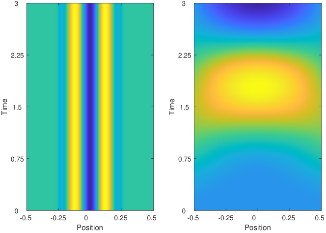
Figure 2: The example of Section 2.1. The potential function $q(x,t)$ (left) and the corresponding solution $u$ of (1) (right).

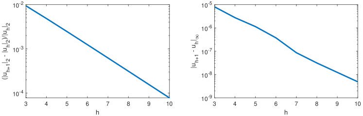
Figure 3: Left: The relative difference $(|u_{h+1}|_{2}-|u_{h}|_{2})/|u_{h}|_{2}$ between $L^{2}$-energies of solutions $u_{h}$ to (19) at successively finer grids in log-scale. Right: the absolute differences $\|u_{h+1}-u_{h}\|_{L^{\infty}}$ evaluated at the common grid points between the successively finer grids in log-scale. We see that the $L^{2}$-energy stays bounded along with finer grids and the values of the numerical solutions converge at the common grid points.

3 Regularized mixed derivatives

As explained in Section 1.2, to recover the potential $q(x,t)$ numerically from the noisy DN map $\widetilde{\Lambda}$,

$$\widetilde{\Lambda}(\varepsilon_{1}f_{1}+\varepsilon_{2}f_{2}):=\Lambda_{q}(\varepsilon_{1}f_{1}+\varepsilon_{2}f_{2})+\mathcal{E},$$

we need to evaluate the mixed derivative

$$\partial^{2}_{\epsilon_{1}\hskip 0.5pt\epsilon_{2}}\big{|}_{\varepsilon_{1}=\varepsilon_{2}=0}\hskip 0.5pt\widetilde{\Lambda}(\varepsilon_{1}f_{1}+\varepsilon_{2}f_{2}).$$

As is well known (and easy to see), numerical differentiation is highly sensitive to noise. Before proceeding to our actual inverse problem, in this section we consider the approach (2) explained in Section 1.2 to compute mixed derivatives approximatively using regularization. We call the result regularized mixed derivative.

Our method derives from the results by Cullum [3], who used Tikhonov regularization to estimate numerical derivatives. For other recent results on numerical differentiation of noisy data we refer to the papers [2, 13] and the references therein.

Our regularized method to compute $\partial^{2}_{\epsilon_{1}\epsilon_{2}}\big{|}_{\varepsilon_{1}=\varepsilon_{2}=0}\widetilde{\Lambda}(\varepsilon_{1}f_{1}+\varepsilon_{2}f_{2})$ is as follows. For this, we consider the problem of finding the mixed derivative $\partial_{s}\partial_{t}g(s,t)$ of a generic function $g\in C^{2}([\alpha,\alpha_{0}]\times[\beta,\beta_{0}])$. By the fundamental theorem of calculus

$$\int_{\alpha}^{x}\partial_{1}g(s,y)\mathrm{d}s=g(x,y)-g(\alpha,y),\quad x\in[\alpha,\alpha_{0}].$$ (23)

For $(x,y)\in[\alpha,\alpha_{0}]\times[\beta,\beta_{0}]$, it then follows that

$$\begin{split}\int_{\beta}^{y}\int_{\alpha}^{x}\partial_{1}\partial_{2}g(s,t)\mathrm{d}s\hskip 0.5pt\mathrm{d}t&=\int_{\beta}^{y}\partial_{2}\big{(}g(x,t)-g(\alpha,t)\big{)}\mathrm{d}t\\ &=g(x,y)-g(\alpha,y)-g(x,\beta)+g(\alpha,\beta),\end{split}$$ (24)

Let $N_{i}$ and $N_{j}$ be positive integers. Let us consider a grid obtained by choosing $N_{i}$ and $N_{j}$ points from $[\alpha,\alpha_{0}]$ and $[\beta,\beta_{0}]$ respectively. Let us denote the discrete values of $\partial_{s}\partial_{t}f(s,t)$ at the grid points by a vector $\mathbf{y}$. The vector $\mathbf{y}$ has thus length $N_{i}N_{j}$. Let us also simply denote by $g$ the vector obtained from the values of $g$ at the grid points. By considering integration as a Riemann sum, the equation (24) in discretized form reads

$$A\mathbf{y}=g,$$ (25)

where the matrix $A$, which is of the size $(N_{i}N_{j})\times(N_{i}N_{j})$, is called the anti-differentiation matrix.

Let us then add noise $\varepsilon_{i,j}$ to the data $g$ by setting

$$\mathbf{g}_{i,j}=g(x_{i},y_{j})-g(\alpha,y_{j})-g(x_{i},\beta)+g(\alpha,\beta)+\varepsilon_{i,j}.$$

In our inverse problem the noise is independent of the grid points and has zero expected value at each grid point. The linear system

$$A\widetilde{\mathbf{y}}=\mathbf{g}$$

can then be solved approximatively via a choice of a regularization method. The approximative solution will then be an approximation of $\partial_{s}\partial_{t}g(s,t)$ at the grid points.

Since the solution to (1) is at least $C^{1}$, we can use this knowledge as an a priori information to help us solve the linear system $A\widetilde{\mathbf{y}}=\mathbf{g}$. Our choice is to use the generalized Tikhonov regularization method (see e.g. the books [10, 26]) written as the minimization problem

$$\mathbf{y}_{\mathrm{reg}}=\mathrm{arg\,min}_{\widetilde{\mathbf{y}}}\big{\{}\|A\widetilde{\mathbf{y}}-\mathbf{g}\|_{L^{2}}+\lambda\|\widetilde{\mathbf{y}}\|_{H^{1}}\big{\}},\quad\lambda>0.$$ (26)

The regularized solution can be obtained by solving

$$(\lambda D^{T}D+A^{T}A)\mathbf{y}_{\mathrm{reg}}=A^{T}\mathbf{g},\quad\lambda>0.$$ (27)

Here the matrix $D$ determines the discretization of the Sobolev $H^{1}$-norm,

$$D^{T}=[I,D_{1}^{T},D_{2}^{T}],$$

where $I$ is the identity matrix, and $D_{1}$ and $D_{2}$ are the difference matrices to the $x$- and $y$-directions respectively. For the matrices $D_{1}$ and $D_{2}$ we used periodic differences. The regularization parameter $\lambda>0$ is chosen experimentally. (The equation (27) can be solved since $D^{T}D=I^{T}I+D_{1}^{T}D_{1}+D_{2}^{T}D_{2}$ is positive definite and $A^{T}A$ is positive semi-definite.)

To demonstrate this approach of numerical differentiation, we calculated regularized mixed derivatives of the functions

$$g(x,y) =\sin(x^{2}+y^{2})$$ (28)

$$g(x,y) =y\sin(x)$$ (29)

over the region $(x,y)\in[-2,2]\times[-2,2]$. The functions were sampled at $35^{2}=1225$ equally spaced grid points. Both measurements were then corrupted by Gaussian noise with standard deviation $\sigma$ equal to $10\,\%$ of the maximum of the function $g$:

$$\sigma=0.1\max_{(x,y)\in[-2,2]^{2}}|g(x,y)|.$$

The resulting regularized derivatives $\partial_{x}\partial_{y}g(x,y)$ are depicted in Figure 4. To demonstrate the effects of regularization, we also included the finite difference approximations of the derivatives in the figures. The effectiveness of regularization is visually striking.

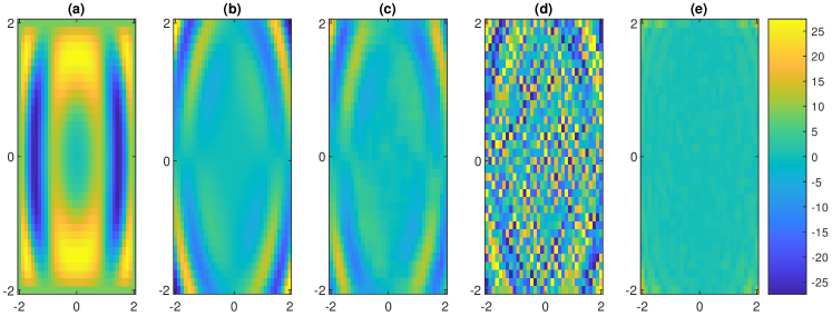
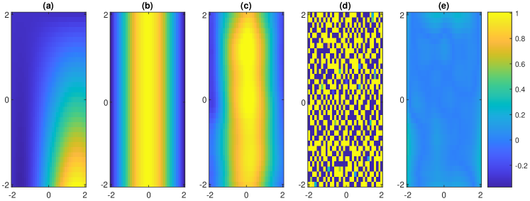
Figure 4: Demonstration of regularization of numerical differentiation of noisy measurements. Example 1, the function (28), on top row and example 2, the function in (29), on bottom row. (a) The function $g$ to be differentiated. (b) The exact derivative $\partial_{x}\partial_{y}g$ of the function $f$. (c) Regularized approximation $\mathbf{y}_{\mathrm{reg}}$ to the derivative $\mathbf{y}$ of the noisy measurement $\mathbf{g}_{i,j}$. (d) Finite difference approximation of the derivative of the noisy measurement $g_{i,j}+\varepsilon_{i,j}$. (e) The absolute difference $|\partial_{x}\partial_{y}g-\mathbf{y}_{\mathrm{reg}}|$. Experimentally chosen regularization parameters $\lambda=0.00001$ and $\lambda=0.01$ have been used in example 1 and 2 respectively.

4 The inverse problem

Let $W$ be the admissible set defined in Section 1 and illustrated in Figure 1. This is a set which can be reached by sending waves from the lateral boundary $\Sigma$ and from which wave signals can also be detected on $\Sigma$. It is the diamond-shaped region in the $(x,t)$-plane given by the conditions

$$t>x-a,$$

$$t<-x+b+T,$$

$$t>-x+b,$$

$$t<x-a+T,$$

$$x\in[a,b]\quad\text{and}\quad t\in[0,T].$$

Let $(x_{0},t_{0})\in W$.

Approach (1): Finite difference approximation of $\partial_{\varepsilon_{1}\varepsilon_{2}}^{2}|_{\varepsilon_{1}=\varepsilon_{2}=0}\widetilde{\Lambda}$. The finite differences (13) are evaluated by using three different boundary value combinations

$$\varepsilon(f_{1}+f_{2}),\ \ \varepsilon f_{1}\ \text{ and }\ \varepsilon f_{2},$$

where $f_{1}$ and $f_{2}$ are as in (9). The measurement data (here for simplicity written without noise) is then obtained as the finite differences

$$\begin{split}F^{L}(t_{j})&=\frac{1}{\varepsilon^{2}}\Big{(}\partial_{\nu}u_{\varepsilon(f_{1}+f_{2})}(a,t_{j})-\partial_{\nu}u_{\varepsilon f_{1}}(a,t_{j})-\partial_{\nu}u_{\varepsilon f_{2}}(a,t_{j})\Big{)},\\ F^{R}(t_{j})&=\frac{1}{\varepsilon^{2}}\Big{(}\partial_{\nu}u_{\varepsilon(f_{1}+f_{2})}(b,t_{j})-\partial_{\nu}u_{\varepsilon f_{1}}(b,t_{j})-\partial_{\nu}u_{\varepsilon f_{2}}(b,t_{j})\Big{)},\end{split}$$ (30)

where $\varepsilon>0$ is chosen experimentally. Here $\partial_{\nu}$ stands for the normal derivatives as in (20).

Approach (2): Obtaining $\partial_{\varepsilon_{1}\varepsilon_{2}}^{2}|_{\varepsilon_{1}=\varepsilon_{2}=0}\widetilde{\Lambda}$ via regularization Let $d>0$ be a small number. We divide the square $[-d,d]^{2}$ into $N_{\varepsilon}\in\mathbb{N}$ equally spaced grid points $(\epsilon_{i},\epsilon_{j})$, and such that the point $(0,0)$ is contained in the grid. The noisy measurements of the DN map are then evaluated at the grid points as

$$\widetilde{\Lambda}_{i,j}:=\Lambda_{q}(\epsilon_{i}f_{1}+\epsilon_{j}f_{2})+\mathcal{E}_{i,j},$$

where $f_{1}$ and $f_{2}$ are as in (9). Let $A$ denote the $N_{\varepsilon}\times N_{\varepsilon}$ anti-differentiation matrix (25). The regularized mixed derivative $F^{L}$ corresponding to measurements on the left side, $x=a$, of the lateral boundary is obtained by solving

$$AF^{L}=\widetilde{\Lambda}|_{x=a}.$$ (31)

This is then an approximation for $\partial_{\varepsilon_{1}\varepsilon_{2}}^{2}\widetilde{\Lambda}(\varepsilon_{1}f_{1}+\varepsilon_{2}f_{2})$ at $x=a$. As explained earlier we consider (31) the minimization problem (26) and use Tikhonov regularization. The regularized mixed derivative $F^{R}$ corresponding to measurements on $x=b$ is obtained similarly. Then

$$(F^{L},F^{R})|_{\varepsilon_{1}=0,\hskip 0.5pt\varepsilon_{2}=0}\text{ is approximation of }\partial_{\varepsilon_{1}\varepsilon_{2}}^{2}|_{\varepsilon_{1}=\varepsilon_{2}=0}\Lambda_{q}.$$

In either of the approaches (1) or (2), let us also define

$$f_{0}^{L}(t_{j}) =H^{\tau=1}((a-x_{0})-(t_{j}-t_{0}))$$

$$f_{0}^{R}(t_{j}) =H^{\tau=1}((b-x_{0})+(t_{j}-t_{0})).$$

Then $f_{0}^{L}$ and $f_{0}^{R}$ correspond to the discretization of the boundary value $\psi$ of the measurement function $v_{0}$ on the left and right side of the lateral boundary respectively. The integral in formula (17),

$$-\frac{1}{2\pi}\int_{\Sigma}\psi\,\partial_{\varepsilon_{1},\varepsilon_{2}}^{2}\Big{|}_{\varepsilon_{1}=\varepsilon_{2}=0}\widetilde{\Lambda}(\varepsilon_{1}f_{1}+\varepsilon_{2}f_{2})\mathrm{d}\Sigma$$

is then our numerical solution to the inverse problem at $(x_{0},t_{0})$. The mixed derivative $\partial_{\varepsilon_{1},\varepsilon_{2}}^{2}|_{\varepsilon_{1}=\varepsilon_{2}=0}\widetilde{\Lambda}(\varepsilon_{1}f_{1}+\varepsilon_{2}f_{2})$ is numerically computed either according to approach (1) or (2). The integral is evaluated numerically as a Riemann sum and we set

$$q^{\mathrm{numerical}}(x_{0},t_{0}):=-\frac{1}{2\pi}\sum_{j=1}^{N_{t}+1}\Big{(}f_{0}^{L}(t_{j})F^{L}(t_{j})+f_{0}^{R}(t_{j})F^{R}(t_{j})\Big{)}\Delta t.$$ (32)

Remark 1.

When studying inverse problems with synthetic data one should keep in mind the so-called inverse crime: If the same model or grid is used for both the forward problem and the inversion, the results of the inversion can in some cases be better than they would be in reality. In our considerations we do not commit an inverse crime, since the reconstruction grid is independent from the grid used in the forward model.

4.1 Choosing the parameters $\tau$ and $\varepsilon$

For the inverse problem we need to choose the parameters $\tau>0$ and $\varepsilon>0$ for the boundary values. We remark that the work [20], given a bound for the noise $\mathcal{E}:H^{s+1}(\Sigma)\to H^{r}(\Sigma)$, with $s\in\mathbb{N}$ and $r\leq s$, computed theoretical values for $\tau$ and $\varepsilon$ that can be used to achieve Hölder stability of the recovery in the inverse problem. In our numerical simulation we however encounter problems using these theoretically values. (Consequently, we expect that the theoretical values for $\tau$ and $\varepsilon$ used in [20] are not optimal in general.)

We choose the parameters $\tau$ and $\varepsilon$ as follows. The parameter $\tau>0$ is chosen by using the following lemma, whose proof can be found from [20].

Lemma 1.

Assume $q$ is a Lipschitz function with Lipschitz constant $L>0$ and let $\tau>0$. The following estimate

$$\left|q(x_{0},t_{0})-\frac{\tau}{\pi}\int_{\mathbb{R}^{2}}q(x,t)\mathrm{e}^{-\tau((x-x_{0})^{2}+(t-t_{0})^{2})}\mathrm{d}x\,\mathrm{d}t\right|\leq\frac{\sqrt{\pi}}{2}L\hskip 0.5pt\tau^{-1/2}$$

holds true for all $(x_{0},t_{0})\in\mathbb{R}^{2}$. In particular, the integral on the left converges uniformly to $q$ when $\tau\to\infty$.

We evaluated the integral in Lemma 1 numerically via Simpson’s quadrature rule for the function

$$q(x,t)=\varphi(5\sqrt{x^{2}+(t-1.5)^{2}})$$

with various different values for $\tau$. The absolute errors are depicted in Figure 5. Evidently larger values of $\tau>0$ result in better approximations. In our simulations, we used the value $\tau=700$.

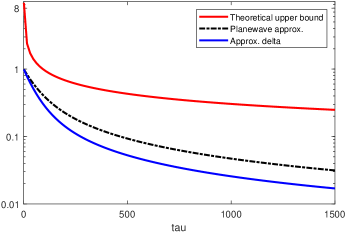
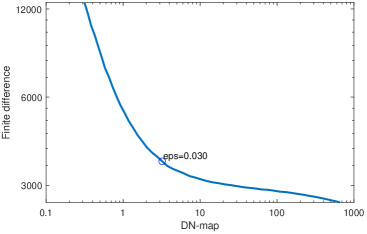
Figure 5: Left: Convergence rate for the integral in Lemma 1 with respect to $\tau\in[0,1500]$. We compare the absolute errors between the integral approximations in sup-norm. Here the red curve depicts the theoretical upper bound $O(\tau^{-1/2})$ given by Lemma 1, the blue curve corresponds to the precise integral of Lemma 1 and the black dot-dash curve depicts the integral of (11). The difference in convergence rates in both pictures is explained by the test function $\chi$ included in the functions $H_{1}^{\tau}$ and $H_{2}^{\tau}$ in the integral (11). Right: The L-curve obtained by comparing the DN maps against the finite differences (30) in $\log\log$-scale. In this case, the “corner” of the curve is located approximatively at $\varepsilon=0.03$.

To numerically compute the derivative $\partial_{\varepsilon_{1}\varepsilon_{2}}^{2}\Lambda_{q}(\varepsilon_{1}f_{1}+\varepsilon_{2}f_{2})$ using finite differences, one has to also make a choice of $\varepsilon$. This is in accordance to the formula (30). Our choice is based on the following heuristic method, often called the L-curve method in the literature [9, 10, 26]. We evaluated the synthetic DN map with multiple values for $\varepsilon\in[0.001,1]$ with logarithmically spaced points. Using these values for $\varepsilon>0$, we then evaluated the corresponding DN maps $\Lambda_{q}(\varepsilon f_{1}+\varepsilon f_{2})$, $\Lambda_{q}(\varepsilon f_{1})$ and $\Lambda_{q}(\varepsilon f_{2})$. The noisy measurements are simulated by adding Gaussian noise with standard deviation equal to

$$\sigma\cdot\mathrm{mean}_{j}(|\partial_{\nu}u(a,t_{j})|+|\partial_{\nu}u(b,t_{j})|)$$ (33)

at the boundary to the synthetic DN map. For this we used Matlab’s randn function and the values $\sigma=0.005,\hskip 0.5pt0.01,\hskip 0.5pt0.015,\hskip 0.5pt0.02,\hskip 0.5pt0.025,\hskip 0.5pt0.03$ (signal-to-noise ratio $42.2$–$57.8\,\mathrm{dB}$). Now, plotting the $L^{2}$-norms of the boundary data:

$$\|\Lambda_{q}(\varepsilon f_{1}+\varepsilon f_{2})\|_{L^{2}(\Sigma)}+\|\Lambda_{q}(\varepsilon f_{1})\|_{L^{2}(\Sigma)}+\|\Lambda_{q}(\varepsilon f_{2})\|_{L^{2}(\Sigma)}$$

against the $L^{2}$-norms of the finite differences $F^{L}(t_{j})$ and $F^{R}(t_{j})$ defined in (30) in $\log\log$-scale, we get the L-shaped curve shown in Figure 5. Heuristically, the reason for the shape of this curve is that when $\varepsilon\to 0$ two things happen: Firstly, the DN map of $\varepsilon f_{1}+\varepsilon f_{2}$ etc. tend to zero. Secondly, due to the presence of noise in the data, the finite differences $F^{L}$ and $F^{R}$ become numerically unstable, increasing their norm. Therefore, one can try to balance between the size of the DN map of $\varepsilon f_{1}+\varepsilon f_{2}$ etc. and the error one makes using the finite differences. Our choice of $\varepsilon$ lies at the “corner” of the L-curve, where both the norm of the measured (noisy) DN map and the norm of the finite differences are small.

Remark 2.

Note that for approach (2) one does not make a choice of a specific $\varepsilon$. Instead, one uses several values of $\varepsilon_{1},\varepsilon_{2}$ on some interval containing $\varepsilon_{1}=\varepsilon_{2}=0$ and then finds the derivative $\partial_{\varepsilon_{1}\varepsilon_{2}}^{2}\widetilde{\Lambda}(\varepsilon_{1}f_{1}+\varepsilon_{2}f_{2})$ as a solution to a minimization problem.

5 Numerical examples

We used the parameters $N_{x}=1000$ and $N_{t}=20000$ to solve the forward problem in the domain $[-0.5,0.5]\times[0,3]$. These choices of $N_{x}$ and $N_{t}$ yield the CFL number $c=0.15$. For the inverse problem, we considered a $N\times N=20\times 20$ equally spaced reconstruction grid of the domain $[-0.4,0.4]\times[1.3,1.7]\subset[-0.5,0.5]\times[0,3]$. As the parameter $\tau$ we use $\tau=700$.
Approach 1: Finite differences When using finite differences to approximate $\partial_{\varepsilon_{1}\varepsilon_{1}}^{2}|_{\varepsilon_{1}=\varepsilon_{2}=0}\widetilde{\Lambda}(\varepsilon_{1}f_{1}+\varepsilon_{2}f_{2})$, we used $\varepsilon\in[0.01,0.2]$ chosen by the L-curve method explained in Section 4.1.
Approach 2: Regularization When using the regularization approach to approximate $\partial_{\varepsilon_{1}\varepsilon_{1}}^{2}|_{\varepsilon_{1}=\varepsilon_{2}=0}\widetilde{\Lambda}(\varepsilon_{1}f_{1}+\varepsilon_{2}f_{2})$ discussed in Sections 3 and 4, we used $15^{2}=225$ equally spaced values $(\epsilon_{m},\epsilon_{n})\in[-0.15,0.15]^{2}$.

We remark that the reconstructions obtained by these two approaches are visually indistinguishable. Approach (1) has the benefit of being simple to implement, but could become unstable depending on the noise. Approach (2) is more involved, but produces more precise mixed derivatives of the noisy measurements.

For the noisy measurements we used Gaussian noise with standard deviations given in (33). These noise levels correspond to signal-to-noise ratios in the range of $42.2$–$57.8\,\mathrm{dB}$ (calculated using Matlab’s snr function from the Signal Processing Package). We mention without details that we got similar results by using uniformly distributed noise with zero mean instead of Gaussian noise.

Let now $\chi_{A}$ be the characteristic function of a set $A$, given by

$$\chi_{A}(x)=\begin{cases}1,&x\in A,\\ 0,&x\not\in A.\end{cases}$$

We test the reconstruction of a potential function from the measurements of noisy DN maps on the following examples:

1. $q(x,t)=\varphi(5\sqrt{x^{2}+(t-1.5)^{2}})$,

2. $q(x,t)=(\sin(4\pi x)+\sin(8\pi t))\varphi(5\sqrt{x^{2}+(t-1.5)^{2}})$,

3. $q(x,t)=\chi_{\mathrm{A=rectangle}}(x,t)$,

4. $q(x,t)=\varphi\Big{(}5\big{(}x-0.15\sin(\frac{\pi}{2}\cos(3\pi t))\big{)}\Big{)}$, (smooth bump oscillating in time).

5. $q(x,t)=\varphi(10x/3)\sin(x)$,

Four of the five examples are intentionally chosen to be time-dependent. This is to study the contrast to inverse problems for the linear Shrödinger wave equation. In these problems time-dependence of the potential can be problematic in both theoretical and numerical reconstructions. The theoretical work [20] does not consider cases where the potential $q$ is discontinuous. We however still test numerically such a case in Ex. 3.

Figures 6–10 show the corresponding reconstructions for the five examples above obtained by evaluating the Riemann sums (32) over the reconstruction grid. In all of the numerical reconstructions, the location and shape of the potential term $q$ is well visible to the eye. In Table 1 we report the values for the absolute error

$$\varepsilon_{\mathrm{abs}}=\max_{j}|q_{j}^{\mathrm{numerical}}-q_{j}^{\mathrm{exact}}|,$$

the absolute relative error

$$\varepsilon_{\mathrm{rel}}=\frac{\max_{j}|q_{j}^{\mathrm{numerical}}-q_{j}^{\mathrm{exact}}|}{\max_{j}|q_{j}^{\mathrm{exact}}|}$$

and the relative error in $L^{2}$-norm

$$\varepsilon_{L^{2}}=\frac{\sqrt{\sum_{j=1}^{N^{2}}(q_{j}^{\mathrm{numerical}}-q_{j}^{\mathrm{exact}})^{2}}}{\sqrt{\sum_{j=1}^{N^{2}}(q_{j}^{\mathrm{exact}})^{2}}}$$

with respect to various noise levels $\sigma$.

	$\sigma$	0	0.005	0.01	0.015	0.02	0.025	0.03
Ex.1	$\varepsilon_{\mathrm{abs}}$	0.088	0.115	0.130	0.135	0.144	0.160	0.166
	$\varepsilon_{\mathrm{rel}}$	0.089	0.116	0.132	0.137	0.146	0.163	0.169
	$\varepsilon_{L^{2}}$	0.121	0.133	0.135	0.139	0.151	0.155	0.163
Ex.2	$\varepsilon_{\mathrm{abs}}$	0.330	0.333	0.349	0.358	0.350	0.335	0.365
	$\varepsilon_{\mathrm{rel}}$	0.240	0.242	0.254	0.261	0.255	0.244	0.266
	$\varepsilon_{L^{2}}$	0.250	0.253	0.259	0.261	0.258	0.255	0.260
Ex.3	$\varepsilon_{\mathrm{abs}}$	0.494	0.519	0.505	0.508	0.520	0.508	0.505
	$\varepsilon_{\mathrm{rel}}$	0.494	0.519	0.505	0.508	0.520	0.508	0.505
	$\varepsilon_{L^{2}}$	0.372	0.378	0.376	0.377	0.378	0.379	0.378
Ex.4	$\varepsilon_{\mathrm{abs}}$	0.299	0.312	0.316	0.317	0.357	0.395	0.460
	$\varepsilon_{\mathrm{rel}}$	0.299	0.312	0.316	0.317	0.357	0.395	0.460
	$\varepsilon_{L^{2}}$	0.206	0.216	0.238	0.256	0.275	0.292	0.315
Ex.5	$\varepsilon_{\mathrm{abs}}$	0.198	0.216	0.221	0.222	0.228	0.223	0.231
	$\varepsilon_{\mathrm{rel}}$	0.260	0.283	0.290	0.290	0.298	0.292	0.302
	$\varepsilon_{L^{2}}$	0.249	0.250	0.252	0.251	0.251	0.254	0.252

Table 1: Comparison of various error quantities between the exact unknown $q^{\mathrm{exact}}$ and the numerical solution $q^{\mathrm{numerical}}$ under different noise levels $\sigma$.

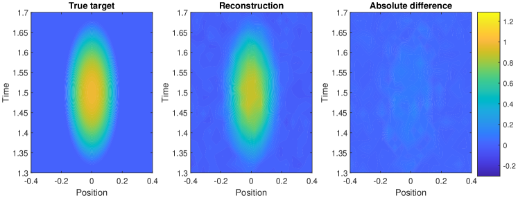
Figure 6: Example 1: Comparison of the true target, supported on the time-interval, and its numerical reconstruction.

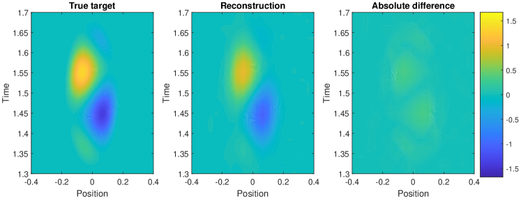
Figure 7: Example 2: Comparison of the true target, which changes sign on the time-interval, and its numerical reconstruction.

Figure 8: Example 3: Comparison of the true target and its numerical reconstruction in the presence of discontinuities. The jump discontinuity of the target is blurred in the reconstruction.

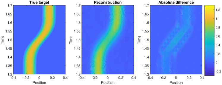
Figure 9: Example 4: Comparison of the true non-compactly supported target target and its numerical reconstruction. The true target is a smooth bump-function, whose location moves in space along time.

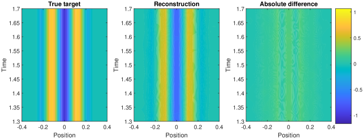
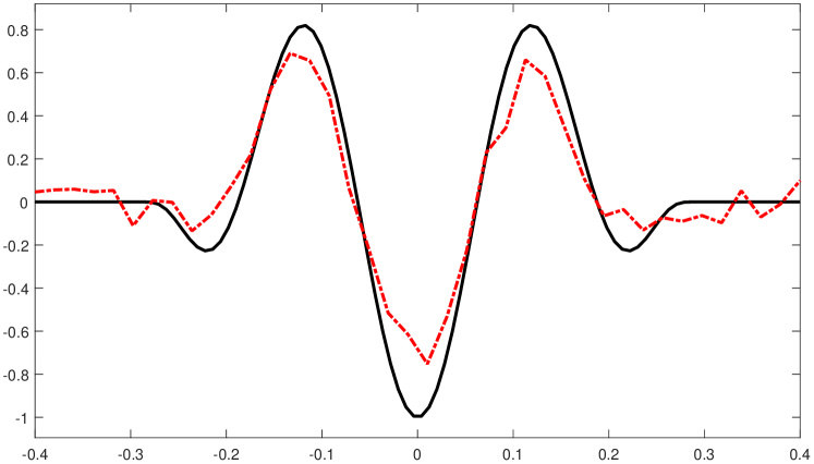
Figure 10: Example 5: Comparison of the true target and its numerical reconstruction in case of time-independent sign-changing target. Top: reconstruction of the potential function in time. Bottom: a cross-section of the true target and its reconstruction at $t_{0}=1.5$ in black and red dot-dash, respectively.

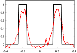
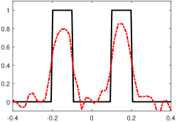
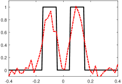
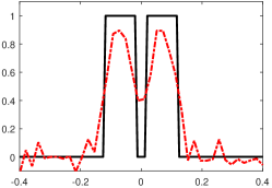
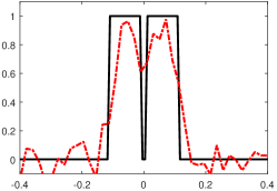
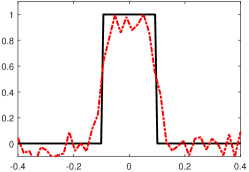
Figure 11: Example 6: To demonstrate the resolution of our numerical method, we consider time-independent potentials $q(x)$ given by the characteristic functions of two small intervals of width $0.1$ at distances $0.4$, $0.3$, $0.2$, $0.14$, $0.12$ and $0.1$ as measured from the center points of the intervals. The cross-sections of the true targets and their reconstructions at fixed time $t_{0}=1.5$ are given in black and red dot-dash, respectively. Two sufficiently far apart target intervals are clearly distinguishable. However, we lose details when the targets are close to each other. There are two reasons for this. Firstly, our approximate plane waves have a finite width of approximately $0.1$ units, which causes loss of small details. Secondly, the potential functions considered are discontinuous and thus the jump discontinuity gets blurred (which is similar to Example 3 in Figure 8).

6 Conclusions

The methods discussed in this paper exploit the nonlinear nature of the wave equation (1). This paper is a numerical demonstration how a nonlinearity helps in inverse problems.

We studied an inverse problem for a one-dimensional nonlinear wave equation of the form $\square u+qu^{2}=0$ from a computational perspective. This was based on the theoretical reconstruction in [20]. The measurement data was the Dirichlet-to-Neumann map on the lateral boundary of the domain. The synthetic DN map was evaluated by numerically solving (1) by using a finite difference scheme (19) and adding Gaussian noise. An example of a solution to the forward problem and its numerical convergence were discussed.

For the inverse problem, we implemented two reconstruction algorithms corresponding to different ways of calculating mixed derivative of the DN map. The first one was based on finite difference approximation (as in [20]) and the other was based on calculating the required mixed derivatives via a regularization method. The regularization method of calculating mixed derivatives numerically were discussed separately. The numerical approximation of the unknown potential was obtained as an integral against the numerical mixed derivative of the nonlinear DN map for specifically chosen boundary values. We presented a heuristic method for choosing the required parameters $\tau$ and $\varepsilon$ of the boundary values.

Finally, multiple examples of reconstructions of potential functions were given, including smooth, discontinuous and time-dependent potentials. The reconstruction was able to identify the location, shape, and size of the potential function.

Acknowledgements

L. P-M. and T. L. were supported by the Academy of Finland (Centre of Excellence in Inverse Modeling and Imaging, grant numbers 284715 and 309963) and by the European Research Council under Horizon 2020 (ERC CoG 770924). T. T was partly supported by the Academy of Finland (Centre of Excellence in Inverse Modeling and Imaging, grant number 312119).

E-mail addresses:
Matti Lassas: matti.lassas@helsinki.fi
Tony Liimatainen: tony.liimatainen@helsinki.fi
Leyter Potenciano-Machado: leyter.m.potenciano@gmail.com
Teemu Tyni: teemu.tyni@utoronto.ca

References

- [1] Balehowsky, T., Kujanpää, A., Lassas, M., and Liimatainen, T. An Inverse Problem for the Relativistic Boltzmann Equation, (2020), arXiv:2011.09312.
- [2] Chartrand, R. Numerical Differentiation of Noisy, Nonsmooth Data, ISRN Applied Mathematics, ID 164564, DOI:10.5402/2011/164564, 2011.
- [3] Cullum, J. Numerical differentiation and regularization, SIAM Journal on Numerical Analysis, vol. 8, 254–265, 1971.
- [4] de Hoop, M., Uhlmann, G. and Wang, Y. Nonlinear responses from the interaction of two progressing waves at an interface. Annales de l’Institut Henri Poincaré C, Analyse non lineaire, 36(2), 347–363, 2019.
- [5] de Hoop, M., Uhlmann, G. and Wang, Y. Nonlinear interaction of waves in elastodynamics and an inverse problem. Mathematische Annalen, 376(1-2), 765–795, 2020.
- [6] Feizmohammadi, A. and Lassas, M. and Oksanen, L., Inverse problems for nonlinear hyperbolic equations with disjoint sources and receivers, Forum Math. Pi, 9, (2021), https://doi.org/10.1017/fmp.2021.11.
- [7] Feizmohammadi, A. and Oksanen, L. Recovery of zeroth order coefficients in non-linear wave equations, To appear in J. Inst. Math. Jussieu, 2020.
- [8] Feizmohammadi, A. and Oksanen, L. An inverse problem for a semi-linear elliptic equation in Riemannian geometries, J. Diff. Equations, 269(6), 4683–4719, 2020.
- [9] Hansen, P. C., Discrete inverse problems: insight and algorithms, SIAM, Philadelphia, 2010.
- [10] Hansen, P. C., Analysis of discrete ill-posed problems by means of the L-curve, SIAM review, 34(4), 561-580, 1992.
- [11] Hintz, P., Uhlmann, G. and Zhai, J. An inverse boundary value problem for a semilinear wave equation on Lorentzian manifolds, Int. Math. Res. Not., rnab088, 2021.
- [12] Hintz, P., Uhlmann, G. and Zhai, J. The Dirichlet-to-Neumann map for a semilinear wave equation on Lorentzian manifolds, arXiv preprint arXiv:2103.08110, 2021.
- [13] Knowles, I. and Renka, R. J. Methods for numerical differentiation of noisy data, Electron. J. Differ. Equ, 21, 235-246, 2014.
- [14] Krupchyk, K. and Uhlmann, G. Partial data inverse problems for semilinear elliptic equations with gradient nonlinearities, to appear in Mathematical Research Letters, arXiv:1909.08122, 2019
- [15] Krupchyk, K. and Uhlmann, G. A remark on partial data inverse problems for semilinear elliptic equations, Proc. Amer. Math. Soc. 148(2), 681–685, 2020.
- [16] Kurylev, Y., Lassas, M., and Uhlmann, G. Inverse problems for Lorentzian manifolds and non-linear hyperbolic equations. Inventiones Mathematicae, 212(3),781–857, 2018. https://doi.org/10.1007/s00222-017-0780-y
- [17] Lai, R-Y., Uhlmann, G., and Yang, Y. Reconstruction of the collision kernel in the nonlinear boltzmann equation, arXiv preprint arXiv:2003.09549, 2020.
- [18] Lassas, M., Liimatainen, T., Lin, Y-H., and Salo, M. Partial data inverse problems and simultaneous recovery of boundary and coefficients for semilinear elliptic equations, arXiv preprint arXiv:1905.02764, 2019.
- [19] Lassas, M., Liimatainen, T., Lin, Y-H. and Salo, M. Inverse problems for elliptic equations with power type nonlinearities, arXiv preprint arXiv:1903.12562.
- [20] Lassas, M, Liimatainen, T., Potenciano-Machado, L., and Tyni, T. Uniqueness and stability of an inverse problem for a semi-linear wave equation, arXiv preprint arXiv:2006.13193 (2020).
- [21] M. Lassas, T. Liimatainen, L. Potenciano-Machado and T. Tyni, Stability estimates for inverse problems for semi-linear wave equations on Lorentzian manifolds, arXiv:2106.12257, (2021).
- [22] L. Shuai, M. Salo and B. Xu, Increasing stability in the linearized inverse Schrö dinger potential problem with power type nonlinearities., arXiv preprint arXiv:2111.13446 (2021).
- [23] Lassas, M., Uhlmann, G. and Wang, Y. Determination of vacuum space-times from the Einstein-Maxwell equations, arXiv preprint arXiv:1703.10704, 2017.
- [24] Lassas, M., Uhlmann, G. and Wang, Y. Inverse Problems for Semilinear Wave Equations on Lorentzian Manifolds, Comm. in Math. Phys., 360, 555–609, 2018.
- [25] Mitchell, A.R. and Griffiths , D.F., The Finite Difference Method in Partial Differential Equations, Wiley, 1980.
- [26] Mueller J. and Siltanen S. Linear and Nonlinear Inverse Problems with Practical Applications, SIAM, Philadelphia, 2012.
- [27] Smith, G.D. Numerical Solution of Partial Differential Equations: Finite Difference Methods, 3rd edition, Clarendon Press, Oxford, 1985.
- [28] L. Shuai, M. Salo and B. Xu, Increasing stability in the linearized inverse Schrö dinger potential problem with power type nonlinearities., arXiv preprint arXiv:2111.13446 (2021).
- [29] Uhlmann, G. and Zhai, J., On an inverse boundary value problem for a nonlinear elastic wave equation, J. Math. Pures Appl., 153, (2021), 114–136, https://doi.org/10.1016/j.matpur.2021.07.005.
- [30] Uhlmann, G. and Zhai, J., Inverse problems for nonlinear hyperbolic equations, Discrete Contin. Dyn. Syst., 41, (2021), No. 1, 455–469, https://doi.org/10.3934/dcds.2020380.
- [31] Wang, Y. and Zhou, T. Inverse problems for quadratic derivative nonlinear wave equations. Comm. PDE, 44(11), 1140–1158, 2019.