A Framework and Benchmark for Deep Batch Active Learning for Regression

Abstract

The acquisition of labels for supervised learning can be expensive. To improve the sample efficiency of neural network regression, we study active learning methods that adaptively select batches of unlabeled data for labeling. We present a framework for constructing such methods out of (network-dependent) base kernels, kernel transformations, and selection methods. Our framework encompasses many existing Bayesian methods based on Gaussian process approximations of neural networks as well as non-Bayesian methods. Additionally, we propose to replace the commonly used last-layer features with sketched finite-width neural tangent kernels and to combine them with a novel clustering method. To evaluate different methods, we introduce an open-source benchmark consisting of 15 large tabular regression data sets. Our proposed method outperforms the state-of-the-art on our benchmark, scales to large data sets, and works out-of-the-box without adjusting the network architecture or training code. We provide open-source code that includes efficient implementations of all kernels, kernel transformations, and selection methods, and can be used for reproducing our results.

Keywords: batch mode deep active learning, regression, tabular data, neural network, benchmark

1 Introduction

While supervised machine learning (ML) has been successfully applied to many different problems, these successes often rely on the availability of large data sets for the problem at hand. In cases where labeling data is expensive, it is important to reduce the required number of labels. Such a reduction could be achieved through various means: First, finding more sample-efficient supervised ML methods; second, applying data augmentation; third, leveraging information in unlabeled data via semi-supervised learning; fourth, leveraging information from related problems through transfer learning, meta-learning, or multi-task learning; and finally, appropriately selecting which data to label. Active learning (AL) takes the latter approach by using a trained model to choose the next data point to label (settles_active_2009). The need to retrain after every new label prohibits parallelized labeling methods and can be far too expensive, especially for neural networks (NNs), which are often slow to train. This problem can be resolved by batch mode active learning (BMAL) methods, which select multiple data points for labeling at once. When the supervised ML method is a deep NN, this is known as batch mode deep active learning (BMDAL) (ren_survey_2021). Pool-based BMDAL refers to the setting where data points for labeling need to be chosen from a given finite set of points.

Supervised and unsupervised ML algorithms choose a model for given data. Multiple models can be compared on the same data using model selection techniques such as cross-validation. Such a comparison increases the training cost, but not the (potentially much larger) cost of labeling data. In contrast to supervised learning, AL is about choosing the data itself, with the goal to reduce labeling cost. However, different AL algorithms may choose different samples, and hence a comparison of $N$ AL algorithms might increase labeling cost by a factor of up to $N$. Consequently, such a comparison is not sensible for applications where labeling is expensive. Instead, it is even more important to properly benchmark AL methods on tasks where labels are cheap to generate or a large number of labels is already available.

In the classification setting, NNs typically output uncertainties in the form of a vector of probabilities obtained through a softmax layer, while regression NNs typically output a scalar target without uncertainties. Therefore, many BMDAL algorithms only apply to one of the two settings. For classification, many BMDAL approaches have been proposed (ren_survey_2021), and there exist at least some standard benchmark data sets like CIFAR-10 (krizhevsky_learning_2009) on which methods are usually evaluated. On the other hand, the regression setting has been studied less frequently, and no common benchmark has been established to the best of our knowledge, except for a specialized benchmark in drug discovery (mehrjou_genedisco_2021). We expect that the regression setting will gain popularity, not least due to the increasing interest in NNs for surrogate modeling (behler_perspective_2016; kutz_deep_2017; raissi_physics-informed_2019; mehrjou_genedisco_2021; lavin_simulation_2021).

1.1 Contributions

In this paper, we investigate pool-based BMDAL methods for regression. Our experiments use fully connected NNs on tabular data sets, but the considered methods can be generalized to different types of data and NN architectures. We limit our study to methods that do not require to modify the network architecture and training, as these are particularly easy to use and a fair comparison to other methods is difficult. We also focus on methods that scale to large amounts of (unlabeled) data and large acquisition batch sizes. Our contributions can be summarized as follows:

1. We propose a framework for decomposing typical BM(D)AL algorithms into the choice of a kernel and a selection method. Here, the kernel can be constructed from a base kernel through a series of kernel transformations. The use of kernels as basic building blocks allows for an efficient yet flexible and composable implementation of our framework, which we include in our open-source code. We also discuss how (regression variants of) many popular BM(D)AL algorithms can be represented in this framework and how they can efficiently be implemented. This gives us a variety of options for base kernels, kernel transformations, and selection methods to combine. Our framework encompasses both Bayesian methods based on Gaussian Processes and Laplace approximations as well as geometric methods.

2. We discuss some alternative options to the ones arising from popular BM(D)AL algorithms: We introduce a novel selection method called LCMD; and we propose to combine the finite-width neural tangent kernel (NTK, jacot_neural_2018) as a base kernel with sketching for efficient computation.

3. We introduce an open-source benchmark for BMDAL involving 15 large tabular regression data sets. Using this benchmark, we compare different selection methods and evaluate the influence of the kernel, the acquisition batch size, and the target metric.

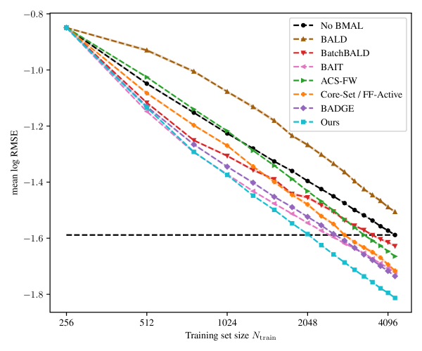
Our newly proposed selection method, LCMD, improves the state-of-the-art in our benchmark in terms of RMSE and MAE, while still exhibiting good performance for the maximum error. The NTK base kernel improves the benchmark accuracy for all selection methods, and the proposed sketching method can preserve this accuracy while leading to significant time gains. Figure 1 shows a comparison of our novel BMDAL algorithm against popular BMDAL algorithms from the literature, which are all implemented in our framework. The code for our framework and benchmark is based on PyTorch (paszke_pytorch_2019) and is publicly available at +rCl+x* https://github.com/dholzmueller/bmdal_reg and will be archived together with the generated data at https://doi.org/10.18419/darus-3394.

Figure 1: This figure shows how fast the averaged errors on our benchmark data sets decrease during BMAL for random selection (no BMAL), BALD (houlsby_bayesian_2011), BatchBALD (kirsch_batchbald_2019), BAIT (ash_gone_2021), ACS-FW (pinsler_bayesian_2019), Core-Set (sener_active_2018), FF-Active (geifman_deep_2017), BADGE (ash_deep_2019), and our method. In LABEL:table:existing_algs_results and LABEL:sec:bmdal:experiments, we specify how the compared methods are built from components explained in Section 4 and LABEL:sec:sel_methods, and discuss further details such as modifications to apply them to regression. For the plot, we start with 256 random training samples and select 256 samples in each of 16 BMAL steps. The lines show the average of the logarithmic RMSE over all 15 benchmark data sets and 20 random splits between the BMAL steps. The shaded area, which is barely visible, corresponds to one estimated standard deviation of the mean estimator, cf. LABEL:sec:appendix:results.

The rest of this paper is structured as follows: In Section 2, we introduce the basic problem setting of BMDAL for tabular regression with fully-connected NNs and introduce our framework for the construction of BMDAL algorithms. We discuss related work in Section 3. We then introduce options to build kernels from base kernels and kernel transformations in Section 4. LABEL:sec:sel_methods discusses various iterative kernel-based selection methods. Our experiments in LABEL:sec:bmdal:experiments provide insights into the performance of different combinations of kernels and selection methods. Finally, we discuss limitations and open questions in LABEL:sec:conclusion. More details on the presented methods and experimental results are provided in the Appendix, whose structure is outlined in LABEL:sec:appendix:overview.

2 Problem Setting

In this section, we outline the problem of BMDAL for regression with fully-connected NNs. We first introduce the regression objective and fully-connected NNs. Subsequently, we introduce the basic setup of pool-based BMDAL as well as our proposed framework.

2.1 Regression with Fully-Connected Neural Networks

We consider multivariate regression, where the goal is to learn a function $f:\mathbb{R}^{d}\to\mathbb{R}$ from data $(\boldsymbol{x},y)\in\mathcal{D}_{\mathrm{train}}\subseteq\mathbb{R}^{d}\times\mathbb{R}$. In the case of NNs, we consider a parameterized function family $(f_{\boldsymbol{\theta}})_{\boldsymbol{\theta}\in\mathbb{R}^{m}}$ and try to minimize the mean squared loss on training data $\mathcal{D}_{\mathrm{train}}$ with $N_{\mathrm{train}}$ samples: +rCl+x* L(θ) & = 1Ntrain ∑_(x, y) ∈D_train (y - f_θ(x))^2 . We refer to the inputs and labels in $\mathcal{D}_{\mathrm{train}}$ as $\mathcal{X}_{\mathrm{train}}$ and $\mathcal{Y}_{\mathrm{train}}$, respectively. Corresponding data sets are often referred to as tabular data or structured data. This is in contrast to data with a known spatiotemporal relationship between the input features, such as image or time-series data, where specialized NN architectures such as CNNs are more successful.

For our derivations and experiments, we consider an $L$-layer fully-connected NN $f_{\boldsymbol{\theta}}:\mathbb{R}^{d}\to\mathbb{R}$ with parameter vector $\boldsymbol{\theta}=(\boldsymbol{W}^{(1)},\boldsymbol{b}^{(1)},\ldots,\boldsymbol{W}^{(L)},\boldsymbol{b}^{(L)})$ and input size $d_{0}=d$, hidden layer sizes $d_{1},\ldots,d_{L-1}$, and output size $d_{L}=1$. The value $\boldsymbol{z}_{i}^{(L)}=f_{\boldsymbol{\theta}}(\boldsymbol{x}_{i}^{(0)})$ of the NN on the $i$-th input $\boldsymbol{x}_{i}^{(0)}\in\mathbb{R}^{d_{0}}$ is defined recursively by

$$\boldsymbol{x}_{i}^{(l+1)}=\varphi(\boldsymbol{z}_{i}^{(l+1)})\in\mathbb{R}^{d_{l+1}},\qquad\boldsymbol{z}_{i}^{(l+1)}=\frac{\sigma_{w}}{\sqrt{d_{l}}}\boldsymbol{W}^{(l+1)}\boldsymbol{x}_{i}^{(l)}+\sigma_{b}\boldsymbol{b}^{(l+1)}\in\mathbb{R}^{d_{l+1}}\leavevmode\nobreak\ .$$ (1)

Here, the activation function $\varphi:\mathbb{R}\to\mathbb{R}$ is applied element-wise and $\sigma_{w},\sigma_{b}>0$ are constant factors. In our experiments, the weight matrices are initialized with independent standard normal entries and the biases are initialized to zero. The factors $\sigma_{w}/\sqrt{d_{l}}$ and $\sigma_{b}$ stem from the neural tangent parametrization (NTP) (jacot_neural_2018; lee_wide_2019), which is theoretically motivated to define infinite-width limits of NNs and is also used in our applications. However, our derivations apply analogously to NNs without these factors. When considering different NN types such as CNNs, it is possible to apply our derivations only to the fully-connected part of the NN or to extend them to other layers as well.

2.2 Batch Mode Active Learning

In a single BMAL step, a BMAL algorithm selects a batch $\mathcal{X}_{\mathrm{batch}}\subseteq\mathbb{R}^{d}$ with a given size $N_{\mathrm{batch}}\in\mathbb{N}$. Subsequently, this batch is labeled and added to the training set. Here, we consider pool-based BMAL, where $\mathcal{X}_{\mathrm{batch}}$ is to be selected from a given finite pool set $\mathcal{X}_{\mathrm{pool}}$ of candidates. Other AL paradigms include membership query AL, where data points for labeling can be chosen freely, or stream-based AL, where data points arrive sequentially and must be immediately labeled or discarded. The pool set can potentially contain information about which regions of the input space are more important than others, especially if it is drawn from the same distribution as the test set. Moreover, pool-based BMAL allows for efficient benchmarking of BMAL methods on labeled data sets by reserving a large portion of the data set for the pool set, rendering the labeling part trivial.

When comparing and evaluating BMDAL methods, we are mainly interested in the following desirable properties:

1. The method should improve the sample efficiency of the underlying NN, even for large acquisition batch sizes $N_{\mathrm{batch}}$ and large pool set sizes $N_{\mathrm{pool}}$, with respect to the downstream application, which may or may not involve the same input distribution as training and pool data.

2. The method should scale to large pool sets, training sets, and batch sizes, in terms of both computation time and memory consumption.

3. The method should be applicable to a wide variety of NN architectures and training methods, such that it can be applied to different use cases.

4. The method should not require modifying the NN architecture and training method, for example by requiring to introduce Dropout, such that practitioners do not have to worry whether employing the method diminishes the accuracy of their trained NN.

5. The method should not require training multiple NNs for a single batch selection since this would deteriorate its runtime efficiency.

6. The method should not require tuning hyperparameters on the downstream application since this would require labeling samples selected with suboptimal hyperparameters.

Property (P1) is central to motivate the use of BMDAL over random sampling of the data and is evaluated for our framework in detail in LABEL:sec:bmdal:experiments and LABEL:sec:appendix:experiments. We only evaluate methods with property (P2) since our benchmark involves large data sets. All methods considered here satisfy (P3) to a large extent. Indeed, although efficient computations are only studied for fully-connected layers here, the considered methods can be simply applied to the fully-connected part of a larger NN. All considered methods satisfy (P4), which also facilitates fair comparison in a benchmark. All our methods satisfy (P5), although our methods can incorporate ensembles of NNs. Although some of the considered methods have hyperparameters, we fix them to reasonable values independent of the data set in our experiments, such that (P6) is satisfied.

Algorithm 1 shows how BMDAL algorithms satisfying (P4) and (P5) can be used in a loop with training and labeling.

Algorithm 1 Basic pool-based BMDAL loop with initial labeled training set $\mathcal{D}_{\mathrm{train}}$, unlabeled pool set $\mathcal{X}_{\mathrm{pool}}$, BMDAL algorithm NextBatch (see Algorithm 2) and a list $L_{\mathrm{batch}}$ of batch sizes.

for AL batch size $N_{\mathrm{batch}}$ in $L_{\mathrm{batch}}$ do

     Train model $f_{\boldsymbol{\theta}}$ on $\mathcal{D}_{\mathrm{train}}$

     Select batch $\mathcal{X}_{\mathrm{batch}}\leftarrow\textsc{NextBatch}(f_{\boldsymbol{\theta}},\mathcal{D}_{\mathrm{train}},\mathcal{X}_{\mathrm{pool}},N_{\mathrm{batch}})$ with $|\mathcal{X}_{\mathrm{batch}}|=N_{\mathrm{batch}}$ and $\mathcal{X}_{\mathrm{batch}}\subseteq\mathcal{X}_{\mathrm{pool}}$

     Move $\mathcal{X}_{\mathrm{batch}}$ from $\mathcal{X}_{\mathrm{pool}}$ to $\mathcal{D}_{\mathrm{train}}$ and acquire labels $\mathcal{Y}_{\mathrm{batch}}$ for $\mathcal{X}_{\mathrm{batch}}$

end for

Train final model $f_{\boldsymbol{\theta}}$ on $\mathcal{D}_{\mathrm{train}}$

wu_pool-based_2018 formulates three criteria by which BMAL algorithms may select batch samples in order to improve the sample efficiency of a learning method:

1. The algorithm should favor inputs that are informative to the model. These could, for example, be those inputs where the model is most uncertain about the label.

2. The algorithm should ensure that the batch contains diverse samples, i.e., samples in the batch should be sufficiently different from each other.

3. The algorithm should ensure representativity of the resulting training set, i.e., it should focus more strongly on regions where the pool data distribution has high density.

Note that (REP) might not be desirable if one expects a significant distribution shift between pool and test data. A challenge in trying to adapt non-batch AL methods to the batch setting is that some non-batch AL methods expect to immediately receive a label for every selected sample. It is usually possible to circumvent this by selecting the $N_{\mathrm{batch}}$ samples with the largest acquisition function scores at once, but this does not enforce (DIV) or (REP).

Algorithm 2 Kernel-based batch construction framework

function KernelNextBatch($f_{\boldsymbol{\theta}},\mathcal{D}_{\mathrm{train}},\mathcal{X}_{\mathrm{pool}},N_{\mathrm{batch}}$)

     $k\leftarrow\textsc{BaseKernel}(f_{\boldsymbol{\theta}})$

     $k\leftarrow\textsc{TransformKernel}(k,\mathcal{D}_{\mathrm{train}})$

     return $\textsc{Select}(k,\mathcal{X}_{\mathrm{train}},\mathcal{X}_{\mathrm{pool}},N_{\mathrm{batch}})$

end function

We propose a framework for assembling BMDAL algorithms that is shown in Algorithm 2 and consists of three components: First, a base kernel $k$ needs to be chosen that should serve as a proxy for the trained network $f_{\boldsymbol{\theta}}$. Second, the kernel can be transformed using various transformations. These transformations can, for example, make the kernel represent posteriors or improve its evaluation efficiency. Third, a selection method is invoked that uses the transformed kernel as a measure of similarity between inputs. When using Gaussian Process regression with a given kernel $k$ as a supervised learning method instead of an NN, the base kernel could simply be chosen as $k$. Note that Select does not observe the training labels directly, however, in the NN setting, these can be implicitly incorporated through kernels that depend on the trained NN.

Example 1.

In Algorithm 2, the base kernel $k$ could be of the form $k(\boldsymbol{x},\tilde{\boldsymbol{x}})=\langle\phi(\boldsymbol{x}),\phi(\tilde{\boldsymbol{x}})\rangle$, where $\phi$ represents the trained NN without the last layer. When interpreting $k$ as the kernel of a Gaussian process, TransformKernel could then compute a transformed kernel $\tilde{k}$ that represents the posterior predictive uncertainty after observing the training data. Finally, Select could then choose the $N_{\mathrm{batch}}$ points $\boldsymbol{x}\in\mathcal{X}_{\mathrm{pool}}$ with the largest uncertainty $\tilde{k}(\boldsymbol{x},\boldsymbol{x})$.

From a Bayesian perspective, our choice of kernel and kernel transformations can correspond to inference in a Bayesian approximation, as we discuss in LABEL:sec:appendix:posterior, while the selection method can correspond to the optimization of an acquisition function. However, in our framework, the same “Bayesian” kernels can be used together with non-Bayesian selection methods and vice versa.

3 Related Work

The field of active learning, also known as query learning or sequential (optimal) experimental design (fedorov_theory_1972; chaloner_bayesian_1995), has a long history dating back at least to the beginning of the 20th century (smith_standard_1918). For an overview of the AL and BMDAL literature, we refer to settles_active_2009; kumar_active_2020; ren_survey_2021; weng_learning_2022.

We first review work relevant to the kernels in our framework, before discussing work more relevant to selection methods, and finally, data sets. More literature related to specific methods is also discussed in Section 4 and LABEL:sec:sel_methods.

3.1 Uncertainty Measures and Kernel Approximations

A popular class of BMDAL methods is given by Bayesian methods since the Bayesian framework naturally provides uncertainties that can be used to assess informativeness. These methods require to use Bayesian NNs, or in other words, the calculation of an approximate posterior distribution over NN parameters. A simple option is to perform Bayesian inference only over the last layer of the NN (lazaro-gredilla_marginalized_2010; snoek_scalable_2015; ober_benchmarking_2019; kristiadi_being_2020). The Laplace approximation (laplace_memoire_1774; mackay_bayesian_1992) can provide a local posterior distribution around a local optimum of the loss landscape via a second-order Taylor approximation. An alternative local approach based on SGD iterates is called SWAG (maddox_simple_2019). Ensembles of NNs (hansen_neural_1990; lakshminarayanan_simple_2017) can be interpreted as a simple multi-modal posterior approximation and can be combined with local approximations to yield mixtures of Laplace approximations (eschenhagen_mixtures_2021) or MultiSWAG (wilson_bayesian_2020). Monte Carlo (MC) Dropout (gal_dropout_2016) is an option to obtain ensemble predictions from a single NN, although it requires training with Dropout (srivastava_dropout_2014). Regarding uncertainty approximations, our considered algorithms are mainly related to exact last-layer methods and the Laplace approximation, as these do not require to modify the training process. daxberger_laplace_2021 give an overview of various methods to compute (approximate) Laplace approximations.

Some recent approaches also build on the neural tangent kernel (NTK) introduced by jacot_neural_2018. khan_approximate_2019 show that certain Laplace approximations are related to the finite-width NTK. wang_deep_2022 and mohamadi_making_2022 propose the use of finite-width NTKs for DAL for classification. wang_neural_2021 use the finite-width NTK at initialization for the streaming setting of DAL for classification and theoretically analyze the resulting method. aljundi_identifying_2022 use a kernel related to the finite-width NTK for DAL. shoham_experimental_2023, borsos_coresets_2020 and borsos_semi-supervised_2021 use infinite-width NTKs for BMDAL and related tasks. han_random_2021 propose sketching for infinite-width NTKs and also evaluate it for DAL. In contrast to these papers, we propose sketching for finite-width NTKs and allow combining the resulting kernel with different selection methods.

3.2 Selection Methods

Besides a Bayesian NN model, a Bayesian BMDAL method needs to specify an acquisition function that decides how to prioritize the pool samples. Many simple acquisition functions for quantifying uncertainty have been proposed (kumar_active_2020). Selecting the next sample where an ensemble disagrees most is known as Query-by-Committee (QbC) (seung_query_1992). krogh_neural_1994 employed QbC for DAL for regression. A more recent investigation of QbC to DAL for classification is performed by beluch_power_2018. pop_deep_2018 combine ensembles with MC Dropout. tsymbalov_dropout-based_2018 use the predictive variance obtained by MC Dropout for DAL for regression. zaverkin_exploration_2021 use last-layer-based uncertainty in DAL for regression on atomistic data. Unlike the other approaches mentioned before, the approach by zaverkin_exploration_2021 can be applied to a single NN trained without Dropout.

Many uncertainty-based acquisition functions do not distinguish between epistemic uncertainty, i.e., lack of knowledge about the true functional relationship, and aleatoric uncertainty, i.e., inherent uncertainty due to label noise. houlsby_bayesian_2011 propose the BALD acquisition function, which aims to quantify epistemic uncertainty only. gal_deep_2017 apply BALD and other acquisition functions to BMDAL for classification with MC Dropout. To enforce diversity of the selected batch, kirsch_batchbald_2019 propose BatchBALD and evaluate it on classification problems with MC Dropout. ash_gone_2021 propose Bait, which also incorporates representativity through Fisher information based on last-layer features, and is evaluated on classification and regression data sets.

Another approach towards BMDAL is to find core-sets that represent $\mathcal{X}_{\mathrm{pool}}$ in a geometric sense. sener_active_2018 and geifman_deep_2017 propose algorithms to cover the pool set with $\mathcal{X}_{\mathrm{batch}}\cup\mathcal{X}_{\mathrm{train}}$ in a last-layer feature space. ash_deep_2019 propose BADGE, which applies clustering in a similar feature space, but includes uncertainty via gradients through the softmax layer for classification. ACS-FW (pinsler_bayesian_2019) can be seen as a hybrid between core-set and Bayesian approaches, trying to approximate the expected log-posterior on the pool set with a core-set, also using last-layer-based Bayesian approximations. Besides Bait, ACS-FW is one of the few approaches that is designed and evaluated for both classification and regression. Our newly proposed selection method LCMD is clustering-based like the k-means++ method used in BADGE, but deterministic.

Many more approaches towards BMDAL exist, and they can be combined with additional steps such as pre-reduction of $\mathcal{X}_{\mathrm{pool}}$ (ghorbani_data_2022) or re-weighting of selected instances (farquhar_statistical_2021). Most of these BMDAL methods are geared towards classification, and for a broader overview, we refer to ren_survey_2021. For (image) regression, ranganathan_deep_2020 introduce an auxiliary loss term on the pool set, which they use to perform DAL. It is unclear, though, to which extent their success is explained by implicitly performing semi-supervised learning.

Since we frequently consider Gaussian Processes (GPs) as approximations to Bayesian NNs in this paper, our work is also related to BMAL for GPs, although in our case the GPs are only used for selecting $\mathcal{X}_{\mathrm{batch}}$ and not for the regression itself. Popular BMAL methods for GPs have been suggested for example by seo_gaussian_2000 and krause_near-optimal_2008.

3.3 Data Sets

In terms of benchmark data sets for BM(D)AL for regression, tsymbalov_dropout-based_2018 use seven large tabular data sets, some of which we have included in our benchmark, cf. LABEL:sec:appendix:data_sets. pinsler_bayesian_2019 use only one large tabular regression data set. ash_gone_2021 use a small tabular regression data set and three image regression data sets, two of which are converted classification data sets. wu_pool-based_2018 benchmarks exclusively on small tabular data sets. zaverkin_exploration_2021 work with atomistic data sets, which require specialized NN architectures and longer training times, and are therefore less well-suited for a large-scale benchmark. ranganathan_deep_2020 use CNNs on five image regression data sets. Recently, a benchmark for BMDAL for drug discovery has been proposed, which uses four counterfactual regression data sets (mehrjou_genedisco_2021). In this paper, we provide an open-source benchmark on 15 large tabular data sets, which includes more baselines and evaluation criteria than evaluations in previous papers.

4 Kernels

In this section, we discuss a variety of base kernels yielding various approximations to a trained NN $f_{\boldsymbol{\theta}_{T}}$, as well as different kernel transformations that yield new kernels with different meanings or simply improved efficiency. In the following, we consider positive semi-definite kernels $k:\mathbb{R}^{d}\times\mathbb{R}^{d}\to\mathbb{R}$. For an introduction to kernels, we refer to the literature (e.g.  steinwart_support_2008). The kernels considered here can usually be represented by a feature map $\phi$ with finite-dimensional feature space, that is, $\phi:\mathbb{R}^{d}\to\mathbb{R}^{d_{\mathrm{feat}}}$ with $k(\boldsymbol{x}_{i},\boldsymbol{x}_{j})=\langle\phi(\boldsymbol{x}_{i}),\phi(\boldsymbol{x}_{j})\rangle$. For a sequence $\mathcal{X}=(\boldsymbol{x}_{1},\ldots,\boldsymbol{x}_{n})$ of inputs, which we sometimes treat like a set $\mathcal{X}\subseteq\mathbb{R}^{d}$ by a slight abuse of notation, we define the corresponding feature matrix

$$\phi(\mathcal{X})=\begin{pmatrix}\phi(\boldsymbol{x}_{1})^{\top}\\ \vdots\\ \phi(\boldsymbol{x}_{n})^{\top}\end{pmatrix}\in\mathbb{R}^{n\times d_{\mathrm{feat}}}$$ (2)

and kernel matrices $k(\boldsymbol{x},\mathcal{X})=(k(\boldsymbol{x},\boldsymbol{x}_{i}))_{i}\in\mathbb{R}^{1\times n}$, $k(\mathcal{X},\mathcal{X})=(k(\boldsymbol{x}_{i},\boldsymbol{x}_{j}))_{ij}\in\mathbb{R}^{n\times n}$, $k(\mathcal{X},\boldsymbol{x})=(k(\boldsymbol{x}_{i},\boldsymbol{x}))_{i}\in\mathbb{R}^{n\times 1}$.

4.1 Base Kernels

We first discuss various options for creating base kernels that induce some notion of similarity on the training and pool inputs. An overview of these base kernels can be found in Table 1.

Base kernel	Symbol	Feature map	Feature space dimension $d_{\mathrm{feat}}$
Linear	$k_{\mathrm{lin}}$	$\phi_{\mathrm{lin}}(\boldsymbol{x})=\boldsymbol{x}$	$d$
NNGP	$k_{\mathrm{nngp}}$	not explicitly defined	$\infty$
full gradient	$k_{\mathrm{grad}}$	$\phi_{\mathrm{grad}}(\boldsymbol{x})=\nabla_{\boldsymbol{\theta}}f_{\boldsymbol{\theta}_{T}}(\boldsymbol{x})$	$\sum_{l=1}^{L}d_{l}(d_{l-1}+1)$
last-layer	$k_{\mathrm{ll}}$	$\phi_{\mathrm{ll}}(\boldsymbol{x})=\nabla_{\tilde{\boldsymbol{W}}^{(L)}}f_{\boldsymbol{\theta}_{T}}(\boldsymbol{x})$	$d_{L}(d_{L-1}+1)$

Table 1: Overview of the introduced base kernels.

4.1.1 Linear Kernel

A very simple baseline for other base kernels is the linear kernel $k_{\mathrm{lin}}(\boldsymbol{x},\tilde{\boldsymbol{x}})=\langle\boldsymbol{x},\tilde{\boldsymbol{x}}\rangle$, corresponding to the identity feature map +rCl+x* ϕ_lin(x) ≔x . It is usually very fast to evaluate but does not represent the behavior of an NN well. Moreover, its feature space dimension depends on the input dimension, and hence may not be suited for selection methods that depend on having high-dimensional representations of the data. A more accurate representation of the behavior of an NN is given by the next kernel:

4.1.2 Full gradient Kernel

If $\boldsymbol{\theta}_{T}$ is the parameter vector of the trained NN, we define +rCl+x* ϕ_grad(x) ≔∇_θ f_θ_T(x) . This is motivated as follows: A linearization of the NN with respect to its parameters around $\boldsymbol{\theta}_{T}$ is given by the first-order Taylor expansion

$$f_{\boldsymbol{\theta}}(\boldsymbol{x})\approx\tilde{f}_{\boldsymbol{\theta}}(\boldsymbol{x})\coloneqq f_{\boldsymbol{\theta}_{T}}(\boldsymbol{x})+\langle\phi_{\mathrm{grad}}(\boldsymbol{x}),\boldsymbol{\theta}-\boldsymbol{\theta}_{T}\rangle\leavevmode\nobreak\ .$$ (3)

If we were to resume training from the parameters $\boldsymbol{\theta}_{T}$ after labeling the next batch $\mathcal{X}_{\mathrm{batch}}$, the result of training on the extended data could hence be approximated by the function $f_{\boldsymbol{\theta}_{T}}+f_{\Delta}$, where $f_{\Delta}$ is the result of linear regression with feature map $\phi_{\mathrm{grad}}$ on the data residuals $(\boldsymbol{x}_{i},y_{i}-f_{\boldsymbol{\theta}_{T}}(\boldsymbol{x}_{i}))$ for $(\boldsymbol{x}_{i},y_{i})\in\mathcal{D}_{\mathrm{train}}\cup\mathcal{D}_{\mathrm{batch}}$.

The kernel $k_{\mathrm{grad}}$ is also known as the (empirical / finite-width) neural tangent kernel (NTK). It depends on the linearization point $\boldsymbol{\theta}_{T}$, but can for certain training settings converge to a fixed kernel as the hidden layer widths go to infinity (jacot_neural_2018; lee_wide_2019; arora_exact_2019). In practical settings, however, it has been observed that $k_{\mathrm{grad}}$ often “improves” during training (fort_deep_2020; long_properties_2021; shan_theory_2021; atanasov_neural_2021), especially in the beginning of training. This agrees with our observations in LABEL:sec:bmdal:experiments and suggests that shorter training might already yield a gradient kernel that allows selecting a good $\mathcal{X}_{\mathrm{batch}}$. Indeed, coleman_selection_2019 found that shorter training and even smaller models can already be sufficient to select good batches for BMDAL for classification.

For fully-connected layers, we will now show that the feature map $\phi_{\mathrm{grad}}$ has an additional product structure that can be exploited to reduce the runtime and memory consumption of a kernel evaluation. For notational simplicity, we rewrite Eq. (1) as +rCl+x* z_i^(l+1) & = ~W^(l+1) ~x_i^(l),
~W^(l+1) ≔ (W(l+1)b(l+1)) ∈R^d_l+1 ×(d_l + 1),  ~x_i^(l) ≔(σwdlxi(l)σb) ∈R^d_l + 1 , with parameters $\boldsymbol{\theta}=(\tilde{\boldsymbol{W}}^{(1)},\ldots,\tilde{\boldsymbol{W}}^{(L)})$. Using the notation from Eq. (4.1.2), we can write

$$\phi_{\mathrm{grad}}(\boldsymbol{x}_{i}^{(0)})=\left(\frac{\,\mathrm{d}\boldsymbol{z}_{i}^{(L)}}{\,\mathrm{d}\tilde{\boldsymbol{W}}^{(1)}},\ldots,\frac{\,\mathrm{d}\boldsymbol{z}_{i}^{(L)}}{\,\mathrm{d}\tilde{\boldsymbol{W}}^{(L)}}\right)=\left(\frac{\,\mathrm{d}\boldsymbol{z}_{i}^{(L)}}{\,\mathrm{d}\boldsymbol{z}_{i}^{(1)}}(\tilde{\boldsymbol{x}}_{i}^{(0)})^{\top},\ldots,\frac{\,\mathrm{d}\boldsymbol{z}_{i}^{(L)}}{\,\mathrm{d}\boldsymbol{z}_{i}^{(L)}}(\tilde{\boldsymbol{x}}_{i}^{(L-1)})^{\top}\right)\leavevmode\nobreak\ .$$ (4)

For a kernel evaluation, the factorization of the weight matrix derivatives can be exploited via +rCl+x* k_grad(x_i^(0), x_j^(0)) & = ∑_l=1^L ⟨dzi(L)dzi(l) (~x_i^(l-1))^⊤, dzj(L)dzj(l) (~x_j^(l-1))^⊤⟩_F
= ∑_l=1^L ⏟⟨~x_i^(l-1), ~x_j^(l-1)⟩_≕k^(l)_in(x_i^(0), x_j^(0)) ⋅⏟⟨dzi(L)dzi(l), dzj(L)dzj(l)⟩_≕k^(l)_out(x_i^(0), x_j^(0)) , since $\langle\boldsymbol{a}\boldsymbol{b}^{\top},\boldsymbol{c}\boldsymbol{d}^{\top}\rangle_{F}=\operatorname{tr}(\boldsymbol{b}\boldsymbol{a}^{\top}\boldsymbol{c}\boldsymbol{d}^{\top})=\operatorname{tr}(\boldsymbol{a}^{\top}\boldsymbol{c}\boldsymbol{d}^{\top}\boldsymbol{b})=\boldsymbol{a}^{\top}\boldsymbol{c}\boldsymbol{d}^{\top}\boldsymbol{b}=\langle\boldsymbol{a},\boldsymbol{c}\rangle\cdot\langle\boldsymbol{b},\boldsymbol{d}\rangle$. This means that $k_{\mathrm{grad}}$ can be decomposed into sums of products of kernels with smaller feature space dimension:

$$k_{\mathrm{grad}}(\boldsymbol{x},\tilde{\boldsymbol{x}})=\sum_{l=1}^{L}k^{(l)}_{\mathrm{in}}(\boldsymbol{x},\tilde{\boldsymbol{x}})\cdot k^{(l)}_{\mathrm{out}}(\boldsymbol{x},\tilde{\boldsymbol{x}})$$ (5)

When using Eq. (4.1.2), the full gradients $\frac{\,\mathrm{d}\boldsymbol{z}_{i}^{(L)}}{\,\mathrm{d}\tilde{\boldsymbol{W}}^{(l)}}$ never have to be computed or stored explicitly. If $\frac{\,\mathrm{d}\boldsymbol{z}_{i}^{(L)}}{\,\mathrm{d}\boldsymbol{z}_{i}^{(l)}}$ and $\tilde{\boldsymbol{x}}_{i}^{(l-1)}$ are already computed and the hidden layers contain $m=d_{1}=\ldots=d_{L-1}$ neurons each, Eq. (4.1.2) reduces the runtime complexity of a kernel evaluation from $\Theta(m^{2}L)$ to $\Theta(mL)$, and similarly for the memory complexity of pre-computed features. In LABEL:sec:kernel_transformations:rp, we will see how to further accelerate this kernel computation using sketching. Efficient computations of $k_{\mathrm{grad}}$ for more general types of layers and multiple output neurons are discussed by novak_fast_2022.

Since $k_{\mathrm{grad}}$ consists of gradient contributions from multiple layers, it is potentially important that the magnitudes of the gradients in different layers are balanced. We achieve this, at least at initialization, through the use of the neural tangent parameterization (jacot_neural_2018). For other NN architectures, however, it might be desirable to re-weight gradient magnitudes from different layers to improve the results obtained with $k_{\mathrm{grad}}$.

4.1.3 Last-layer Kernel

A simple and rough approximation to the full-gradient kernel is given by only considering the gradient with respect to the parameters in the last layer: +rCl+x* ϕ_ll(x) ≔∇_~W^(L) f_θ_T(x) . From Eq. (4), it is evident that in the single-output regression case that we are considering, $\phi_{\mathrm{ll}}(\boldsymbol{x}_{i}^{(0)})$ is simply the input $\tilde{\boldsymbol{x}}_{i}^{(L-1)}$ to the last layer of the NN. The latter formulation can also be used in the multi-output setting, and versions of it (with $\boldsymbol{x}_{i}^{(L-1)}$ instead of $\tilde{\boldsymbol{x}}_{i}^{(L-1)}$) have been frequently used for BMDAL (sener_active_2018; geifman_deep_2017; pinsler_bayesian_2019; ash_deep_2019; zaverkin_exploration_2021; ash_gone_2021).

4.1.4 Infinite-width NNGP

It has been shown that as the widths $d_{1},\ldots,d_{L-1}$ of the hidden NN layers converge to infinity, the distribution of the initial function $f_{\boldsymbol{\theta}_{0}}$ converges to a Gaussian Process with mean zero and a covariance kernel $k_{\mathrm{nngp}}$ called the neural network Gaussian process (NNGP) kernel (neal_priors_1994; lee_deep_2018; matthews_gaussian_2018). This kernel depends on the network depth, the used activation function, and details such as the initialization variance and scaling factors like $\sigma_{w}$. In our experiments, we use the NNGP kernel corresponding to the employed NN setup, for which the formulas are given in LABEL:sec:appendix:nngp.

As mentioned above, there exists an infinite-width limit of $k_{\mathrm{grad}}$, the so-called neural tangent kernel (jacot_neural_2018). We decided to omit it from our experiments in LABEL:sec:appendix:experiments after preliminary experiments showed similarly bad performance as for the NNGP.

4.2 Kernel Transformations

The base kernels introduced in Section 4.1 are constructed such that kernel regression with these kernels serves as a proxy for regression with the corresponding NN. By using kernels, we can model interactions $k(\boldsymbol{x},\tilde{\boldsymbol{x}})$ between two inputs, which is crucial to incorporate diversity (DIV) into the selection methods. However, this is not always sufficient to apply a selection method. For example, sometimes we want the kernel to represent uncertainties of the NN after observing the data, or we want to reduce the feature space dimension to render selection more efficient. Therefore, we introduce various ways to transform kernels in this section. When applying transformations $T_{1},\ldots,T_{n}$ in this order to a base kernel $k_{\mathrm{base}}$, we denote the transformed kernel by $k_{\mathrm{base}\to T_{1}\to T_{2}\to\ldots\to T_{n}}$. Of course, we can only cover selected transformations relevant to our applications, and other transformations such as sums or products of kernels are possible as well.

Notation	Description	$d_{\mathrm{pre}}$	$d_{\mathrm{post}}$	Configurable $\sigma^{2}$?
$k_{\to\operatorname{scale}(\mathcal{X})}$	Rescale kernel to normalize mean $k(\boldsymbol{x},\boldsymbol{x})$ on $\mathcal{X}$	any	$d_{\mathrm{pre}}$	no
$k_{\to\operatorname{post}(\mathcal{X},\sigma^{2})}$	GP posterior covariance after observing $\mathcal{X}$	any	$d_{\mathrm{pre}}$	yes
$k_{\to\mathcal{X}}$	Short for $k_{\to\operatorname{scale}(\mathcal{X})\to\operatorname{post}(\mathcal{X},\sigma^{2})}$	any	$d_{\mathrm{pre}}$	yes
$k_{\to\operatorname{sketch}(p)}$	Sketching with $p$ features	$<\infty$	$p$	no
$k_{\to\operatorname{ens}(N_{\mathrm{ens}})}$	Sum of kernels for $N_{\mathrm{ens}}$ ensembled networks	any	$N_{\mathrm{ens}}d_{\mathrm{pre}}$	no
$k_{\to\operatorname{acs-grad}}$	Gradient-based kernel from pinsler_bayesian_2019	any	$d_{\mathrm{pre}}^{2}$	yes
$k_{\to\operatorname{acs-rf}(p)}$	Kernel from pinsler_bayesian_2019 with $p$ random features	$<\infty$	$p$	yes
$k_{\to\operatorname{acs-rf-hyper}(p)}$	Kernel from pinsler_bayesian_2019 with $p$ random features and hyperprior on $\sigma^{2}$	$<\infty$	$p$	no

Table 2: Overview of our considered kernel transformations that can be applied to a kernel $k$. Here, $d_{\mathrm{pre}}$ refers to the feature space dimension of $k$ and $d_{\mathrm{post}}$ refers to the feature space dimension after the transformation. Moreover, $\sigma^{2}$ refers to the assumed noise variance in the GP model.

4.2.1 Scaling

For a given kernel $k$ with feature map $\phi$ and scaling factor $\lambda\in\mathbb{R}$, we can construct the kernel $\lambda^{2}k$ with feature map $\lambda\phi$. This scaling can make a difference if we subsequently consider a Gaussian Process (GP) with covariance function $\lambda^{2}k$. In this case, $\lambda^{2}k(\boldsymbol{x},\tilde{\boldsymbol{x}})$ describes the covariance between $f(\boldsymbol{x})$ and $f(\tilde{\boldsymbol{x}})$ under the prior distribution over functions $f$. Since we train with normalized labels, $N_{\mathrm{train}}^{-1}\sum_{y\in\mathcal{Y}_{\mathrm{train}}}y_{i}^{2}\approx 1$, we would like to choose the scaling factor $\lambda$ such that $N_{\mathrm{train}}^{-1}\sum_{\boldsymbol{x}\in\mathcal{X}_{\mathrm{train}}}\lambda^{2}k(\boldsymbol{x},\boldsymbol{x})=1$. Therefore, we propose the automatic scale normalization +rCl+x* k_→scale(X_train)(x, ~x) ≔λ^2 k(x, ~x),   λ≔(1Ntrain ∑_x∈X_train k(x, x))^-1/2 .

4.2.2 Gaussian Process Posterior Transformation

For a given kernel $k$ with corresponding feature map $\phi$, we can consider a Gaussian Process (GP) with kernel $k$, which is equivalent to a Bayesian linear regression model with feature map $\phi$: In feature space, we model our observations as $y_{i}=\boldsymbol{w}^{\top}\phi(\boldsymbol{x}_{i})+\varepsilon_{i}$ with weight prior $\boldsymbol{w}\sim\mathcal{N}(\boldsymbol{0},\boldsymbol{I})$ and i.i.d. observation noise $\varepsilon_{i}\sim\mathcal{N}(0,\sigma^{2})$. The random function $f(\boldsymbol{x}_{i})\coloneqq\boldsymbol{w}^{\top}\phi(\boldsymbol{x}_{i})$ now has the covariance function $\operatorname{Cov}(f(\boldsymbol{x}_{i}),f(\boldsymbol{x}_{j}))=\phi(\boldsymbol{x}_{i})^{\top}\phi(\boldsymbol{x}_{j})=k(\boldsymbol{x}_{i},\boldsymbol{x}_{j})$.

It is well-known, see e.g. Section 2.1 and 2.2 in bishop_pattern_2006, that the posterior distribution of a Gaussian process after observing the training data $\mathcal{D}_{\mathrm{train}}$ with inputs $\mathcal{X}_{\mathrm{train}}$ is also a Gaussian process with kernel +rCl+x* & k_→post(X_train, σ^2)(x, ~x)
≔ Cov(f(x), f(~x) ∣X_train, Y_train)
= k(x, ~x) - k(x, X_train) (k(X_train, X_train) + σ^2 I)^-1 k(X_train, ~x) 
=see below ϕ(x)^⊤(σ^-2 ϕ(X_train)^⊤ϕ(X_train) + I)^-1 ϕ(~x)
= σ^2 ϕ(x)^⊤(ϕ(X_train)^⊤ϕ(X_train) + σ^2 I)