Confidence Dimension for Deep Learning based on Hoeffding Inequality and Relative Evaluation

Abstract

Research on the generalization ability of deep neural networks (DNNs) has recently attracted a great deal of attention. However, due to their complex architectures and large numbers of parameters, measuring the generalization ability of specific DNN models remains an open challenge. In this paper, we propose to use multiple factors to measure and rank the relative generalization of DNNs based on a new concept of confidence dimension ($CD$). Furthermore, we provide a feasible framework in our $CD$ to theoretically calculate the upper bound of generalization based on the conventional Vapnik-Chervonenk dimension (VC-dimension) and Hoeffding’s inequality. Experimental results on image classification and object detection demonstrate that our $CD$ can reflect the relative generalization ability for different DNNs. In addition to full-precision DNNs, we also analyze the generalization ability of binary neural networks (BNNs), whose generalization ability remains an unsolved problem. Our $CD$ yields a consistent and reliable measure and ranking for both full-precision DNNs and BNNs on all the tasks.

1 Introduction

Deep neural networks (DNNs) contribute significantly to many computer vision tasks over the past decade. However, most DNNs are heavily over-parameterized, which means that the models can achieve near-perfect performance on the training data but have a performance gap on the test data. Measuring the generalization ability is complex. This raises a fundamental question: can we fairly and objectively evaluate the generalization ability of a deep learning model?

Theoretical research on the image classification capacity of shallow models starts with Vapnik-Chervonenkis Dimension (VC-dimension) Vapnik and Chervonenkis (1971). Taking the data distribution into account, Bartlett et al. Bartlett and Mendelson (2002) further proposes the Rademacher complexity, a stricter generalization error bound.

The training of DNNs is more complicated and involves solving nonconvex optimization problems in a very high-dimensional space. Moreover, it is difficult to find the global minimum of DNNs analytically. Previous works Dziugaite and Roy (2016) have shown that there is a degree of correlation between the optimizer and the generalization ability of DNNs. Inspired by this, Fort et al. Fort et al. (2019) proposes a gradient alignment measure to understand the generalization. However, the optimizer is not the only factor that affects the generalization ability. For example, training different network architectures with the same optimizer may lead to other generalization errors. Furthermore, batch size and regularization techniques such as dropout Srivastava et al. (2014), weight decay, and early stopping also influence the generalization ability. Those regularization techniques lower the model’s complexity and therefore affect the generalization.

Based on these observations, the generalization of DNNs should consider both the network architecture and the optimization. Due to finite sampling set, traditional VC-dimension can only produce quite loose generalization bounds, which are unsuitable to describe DNNs with more parameters than training samples Valle-Pérez and Louis (2020); Zhang et al. (2017). Tighter generalization bounds Neyshabur et al. (2019); Valle-Pérez and Louis (2020) have been proposed to understand the generalization ability of deep models better. However, these generalization bounds are still impractical for real applications because of their restrictive assumptions. For example, Valle et al. Valle-Perez et al. (2018) ignores the effects of different training “tricks” on the generalization. Furthermore, Neyshabur et al. Neyshabur et al. (2019) limits the architecture to two-layer networks, and Valle et al. Valle-Pérez and Louis (2020) restricts the studied image classification tasks to binary problems. Moreover, previous methods based on VC-dimension often offer an unstable explanation and occasionally show trends opposite the actual error. Previous bound predictions increase with the increasing training set size, while the measured error decreases Nagarajan and Kolter (2019). As a result, for real applications only when a finite training sample set is available for the VC-dimension calculation, a theoretical upper bound for generalization will provide a guidance to analyze DNNs from a pragmatic perspective.

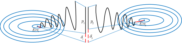
Figure 1: The illustration of Confidence Dimension. The traditional VC-dimension estimation ignores the process of optimization, which lead to different measure results ($p_{1}$ and $p_{2}$) for the VC-dimension of the same model. To address the issue, we theoretically calculate the upper bound of the VC-dimension based on a correction term ($\delta_{1}$ and $\delta_{2}$) which is positively related to the training error for a stable generalization estimation.

So far, there has not been any effective method to measure generalization. In this paper, we propose a new concept of confidence dimension ($CD$) based on VC-dimension and Hoeffding’s inequality to fairly evaluate the generalization ability of DNNs, by considering both the network architecture and the optimization process in a unified framework, as shown in Fig. 1. Many factors are not taken into account in the VC-dimension Zhang et al. (2017). Now we consider inputs and process of optimization as a correction term to obtain the upper bound of generalization, so as to ensure that the generalization of models are compared within a unified and relatively completed framework. It also can be used to measure the generalization of models on a unified scale under different experimental conditions. We investigate the generalization evaluation based on a relative assessment of different DNN models, i.e., focus on the $CD$ ranking consistency of DNN models across different situations, which is more practical than existing methods Bartlett and Mendelson (2002); Vapnik and Chervonenkis (1971). We take two steps to establish an upper bound for generalization, leading to our confidence dimension ($CD$), and provide explanatory power for DNNs. First, DNN models are trained on randomly and accurately labeled data to calculate the VC-dimension. Then, based on Hoeffding’s inequality, we calculate the corrected term of generalization by considering the optimization process Dziugaite et al. (2020) into calculating the $CD$. According to the law of large numbers, the $CD$ will become stable by performing large numbers of experiments.

We demonstrate the rationale of our method theoretically and experimentally. We first provide a theoretical derivation of the upper bound of generalization based on the VC-dimension and Hoeffding’s inequality. Then, we further extensively validate the generalization bound $CD$ by cross-tasks, including image classification and object detection. Moreover, different from existing works analyzing the generalization ability only for full-precision models, we also evaluate the generalization ability for binary neural networks (BNNs). BNNs Gu et al. (2019); Hubara et al. (2016); Liu et al. (2020) are among the most compressed deep models and are worth exploring their generalization performance, which quantize weights and features to single bits and have attracted intense interest for their excellent computation acceleration and model compression. The main contributions of this paper are as follows:

• We propose a confidence dimension ($CD$) to measure the relative generalization ability of deep models and provide a new approach for generalization prediction.

• We show that theoretically, our $CD$ is the upper bound of generalization based Hoeffding’s inequality, which is more feasible than conventional measures when only a data-driven method is available to measure the generalization ability of DNNs.

• We extensively validate the performance of our $CD$ by cross-tasks, including image classification and object detection, BNNs and full-precision DNNs, which are consistent with the theoretical results. The $CD$ measure of a DNN is stable for various tasks and is potentially a useful tool to evaluate the generation for DNNs.

2 Related Work

The VC-dimension Vapnik and Chervonenkis (1971) provides a general measure of the complexity of traditional models and reflects their learning ability. It is closely related to the generalization performance of the underlying models. To guarantee good generalization performance, we expect a novelty dimension to give a tight bound on the expected error. Unfortunately, the VC-dimension has practical limitations when applied to the generalization of DNNs. Contrary to VC-dimension theory, decreasing the number of parameters in DNNs may achieve a better generalization performance. This is primarily because having more parameters than the number of training examples usually results in a loose generalization bound based on the VC-dimension Zhang et al. (2017). Furthermore, different optimizers or regularization techniques have an influence on the optimization process and lower the model complexity, affecting the generalization Srivastava et al. (2014). Gintare et al. Dziugaite et al. (2020) argues that generalization measures should instead be evaluated within the framework of distributional robustness. Bengio et al. Jiang et al. (2019) confirms that implicit regularization and optimizer influence the model in the same trend, i.e., the process of optimization is a comprehensive measurement of optimizer and regularization.

Existing works mainly focus on estimating a tighter generalization bound to understand the generalization ability of DNN models better. Sun et al. Sun et al. (2016) expects the generalization error to be bounded by an empirical margin error plus the Rademacher Average term. Instead, works Valle-Pérez and Louis (2020) prefer the PAC-Bayes bounds. Valle et al. Valle-Perez et al. (2018) computes the PAC-Bayes generalization error bounds using the Gaussian process approximation of the prior over functions. Furthermore, Valle et al. Valle-Pérez and Louis (2020) proposes a marginal-likelihood PAC-Bayes bound under the assumption of a power-law asymptotic behavior with training set size.

Yet strong assumptions are still key bottlenecks preventing those generalization bounds from practical use. To evaluate the generalization of DNNs more flexibly, we propose a new measurement method that comprehensively considers the model’s structure, optimization, and other training details like the training set size. In this case, we can compare the upper bound of the generalization ability between models in practical applications.

3 Measuring Relative Generalization Ability

Our goal is to present a flexible framework to compare the generalization ability of different networks. Based on randomization tests also used in VC-dimension, we calculate the confidence dimension ($CD$) to measure the models’ generalization performance. In the following, we will introduce VC-dimension, $CD$, and then analyze $CD$ theoretically.

3.1 VC-dimension Estimation

Let $\mathcal{H}$ be a hypothetical space, and $\mathcal{X}=\left\{x_{1},x_{2},...,x_{m}\right\}$ be a sampling set with size $m$. Each hypothesis $h$ in $\mathcal{H}$ marks a sample in $\mathcal{X}$, and the result is expressed as:

$$h|\mathcal{X}=\left\{h(x_{1}),h(x_{2}),...,h(x_{m})\right\}.$$ (1)

As the size of sample $m$ increases, the number of corresponding examples in $\mathcal{X}$ may also increase. For $m\in N$, the growth function is defined as:

$$\Pi_{\mathcal{H}}(m)=\max_{{x_{1},...,x_{m}}\subseteq\mathcal{X}}|\left\{h(x_{1}),h(x_{2}),...,h(x_{m})|h\in\mathcal{H}\right\}|.$$ (2)

The growth function $\Pi_{\mathcal{H}}(m)$ represents the maximum number of possible results that can be labeled with the hypothesis space $\mathcal{H}$ for $m$ examples. The greater the number of possible results that $\mathcal{H}$ can label for these examples, the stronger the expression ability of $\mathcal{H}$. In deep learning, the DNN is the hypothesis space $\mathcal{H}$.

Now let us double the number of sample sets $\mathcal{X}=\{x_{1},...,x_{m},x_{m+1},...,x_{2m}\}$ and generate subsets $\mathcal{X}_{1}=\{x_{1},...,x_{m}\}$ and $\mathcal{X}_{2}=\{x_{m+1},...,x_{2m}\}$. The risk of $\mathcal{X}$ in the deep learning model is defined as Vapnik and Chervonenkis (1971):

$$v(\mathcal{X})=\frac{1}{2m}\sum_{i=0}^{2m}|y_{i}-f(x_{i})|,$$ (3)

where $y_{i}$ is the label of the dataset and $f(x_{i})$ is the classification results of the model. Therefore, the risks of the two subsets are:

$$v(\mathcal{X}_{1})=\frac{1}{m}\sum_{i=0}^{m}|y_{i}-f(x_{i})|,$$ (4)

$$v(\mathcal{X}_{2})=\frac{1}{m}\sum_{i=m+1}^{2m}|y_{i}-f(x_{i})|.$$

According to previous work Vapnik and Chervonenkis (1971), the difference between the two risks $v(\mathcal{X}_{1})$ and $v(\mathcal{X}_{2})$ is positively correlated with the sample set size $m$.

$${p}=\sup\{v(\mathcal{X}_{1})-v(\mathcal{X}_{2})\}\propto m,$$ (5)

$\sup$ denotes the upper limit, which can be obtained by maximizing:

$$\frac{1}{m}\sum_{i=1}^{m}|y_{i}-f(x_{i})|-\frac{1}{m}\sum_{i={m}+1}^{2m}|y_{i}-f(x_{i})|$$ (6)

$$=(1-\frac{1}{m}\sum_{i=1}^{m}|\tilde{y}_{i}-f(x_{i})|)-\frac{1}{m}\sum_{i={m}+1}^{2m}|{y_{i}}-f(x_{i})|,$$

which is equivalent to :

$${p}=\inf\{(\frac{1}{m}\sum_{i=1}^{m}|\tilde{y}_{i}-f(x_{i})|+\frac{1}{m}\sum_{i={m}+1}^{2m}|y_{i}-f(x_{i})|)\},$$ (7)

where $\tilde{y}_{i}$ is the incorrect label of the dataset, $\inf$ denotes lower limit. When the sample set size $m$ is the same, VC-demision is proportional to ${p}$. The result of $p$ will be normalized. There exist ${\zeta,\varepsilon}\in(0,\infty)$, such that the form of VC-dimension is shown below Vapnik and Chervonenkis (1971):

$$VC\propto\frac{\zeta}{e^{-\frac{m\varepsilon^{2}}{8}}}{p}.$$ (8)

We can know that ${p}$ is a measure of VC-dimension, which can be used to rank VC-dimension of different models. The minimum value in Eq. 7 cannot be easily estimated because of the huge complexity of deep learning models. We can only approximate the global minimum with a local minimum, which is actually related to the used optimizer. Furthermore, finding the maximum number of shattered samples still remains an open problem. As a result, we can only obtain an inaccurate generalization measure for DNNs by the method of VC-dimension.

3.2 Confidence Dimension

We consider multiple elements to define a new measure $CD$, which can provide a much more stable measure than VC-dimension. To this end, we calculate the correction term $\delta$ of generalization, which can be used to bound the generalization ability. $\delta$ is estimated as:

$$\delta=\alpha\sqrt{\frac{\ln(2+Err)}{m}},$$ (9)

where $Err$ denotes the training error for the sample set $\mathcal{X}$, $\alpha$ denotes the coefficient of correction terms, and $m$ is the size of $\mathcal{X}$. We then define the confidence dimension ($CD$) as:

$$CD=\sup\{v(\mathcal{X}_{1})-v(\mathcal{X}_{2})\}+\delta,$$ (10)

in order to ensure $CD\in[0,1]$, $CD$ will be normalized. The advantages of our measure lie in that: 1) Our $CD$ can be more consistent than VC-dimension. Based on our theoretical investigation, we show that our measure is the upper bound of generalization based on the VC-dimension, which might have a tighter constraint; 2) Our $CD$ can effectively measure the relative generalization ability of different DNNs based on a finite sample size.

Theorem 1.

The Confidence Dimension is an upper bound of the generalization ability of any model with a probability of

$$1-\frac{1}{(2+Err)^{4}}$$

where $Err$ is training error.

Proof. We denote $\hat{p}_{i}$ as the normalized optimal value for the $i^{th}$ batch of independent and identically distributed samples, which is the infimum calculated by Eq. 7. We also define:

$$\hat{p}=\frac{\sum\hat{p}_{i}}{m},$$

where $m$ is the number of input samples. For easy proof our result, we reasonably assume $\hat{p}$ as the probability measure of obtaining the upper bound of generalization. Due to the independence of $CD_{i}$ (in the $i^{th}$ batch), we can get Eq. 11 based on the Hoeffding’s inequality Dubhashi and Panconesi (2009):

$$\mathbb{E}[e^{\lambda CD}]=\mathbb{E}[e^{\frac{\lambda}{m}\sum_{i}[CD_{i}]}]$$ (11)

$$=\prod_{i}\mathbb{E}({e^{\frac{\lambda}{m}CD_{i}}})=\prod_{i}(\hat{p}_{i}e^{\frac{\lambda}{m}}+\hat{q}_{i})$$

$$\leq(\frac{\sum_{i}(\hat{p}_{i}e^{\frac{\lambda}{m}}+\hat{q}_{i})}{m})^{m}=(\hat{p}e^{\frac{\lambda}{m}}+\hat{q})^{m},$$

where $\hat{q}_{i}=1-\hat{p}_{i}$ and $\hat{q}=1-\hat{p}$. Given Markov’s inequality, we have:

$$P[CD\geq\hat{p}+\delta] =P[\frac{1}{m}\sum_{i}(CD_{i}-\hat{p}_{i})\geq\delta]$$ (12)

$$=P[e^{\frac{\lambda}{m}\sum_{i}(CD_{i}-\hat{p}_{i})}\geq e^{\lambda\delta}]$$

$$\leq\frac{\mathbb{E}[e^{\frac{\lambda}{m}\sum_{i}(CD_{i}-\hat{p}_{i})}]}{e^{\lambda\delta}}.$$

We also have $1+x\leq e^{x}\leq 1+x+x^{2},$ when $0\leq|x|\leq 1$. We thus have $\mathbb{E}[e^{\frac{\lambda}{m}\sum_{i}(CD_{i}-\hat{p}_{i})}]$ in Eq. 12, which can be further approximated as:

$$\mathbb{E}[e^{\frac{\lambda}{m}\sum_{i}(CD_{i}-\hat{p}_{i})}]$$ (13)

$$=\prod_{i}\mathbb{E}[e^{\frac{\lambda}{m}(CD_{i}-\hat{p}_{i})}]$$

$$\leq\prod_{i}\mathbb{E}[1+\frac{\lambda}{m}(CD_{i}-\hat{p}_{i})+(\frac{\lambda}{m})^{2}(CD_{i}-\hat{p}_{i})^{2}]$$

$$=\prod_{i}(1+(\frac{\lambda}{m})^{2}v_{i}^{2})\leq e^{(\frac{\lambda}{m})^{2}v^{2}},$$

where $v_{i}$ denotes the variance of $CD_{i}$, $v$ denotes the variance of $CD$. Combining Eq. 12 and Eq. 13 gives $P[CD\geq\hat{p}+\delta]\leq\frac{e^{(\frac{\lambda}{m})^{2}v^{2}}}{e^{\lambda\delta}}$. Since $\lambda$ is a non-negative constant and $CD\in[0,1]$,according to the root formula, it can be obtained by transforming values such that $P[CD\geq\hat{p}+\delta]\leq e^{-2m\delta^{2}}$ when $m\geq 8$. From the symmetry of the distribution, we have $P[CD<\hat{p}-\delta]\leq e^{-2m\delta^{2}}$. Finally, we get the inequality:

$$P[|CD-\hat{p}|\leq\delta]\geq 1-2e^{-2m\delta^{2}},$$ (14)

where $\hat{p}$ is is the normalized theoretical VC-dimension value. We guarantee that $\delta$ decrease as the size of the input samples increases. Therefore, we choose $\alpha\sqrt{\frac{\ln{(2+Err)}}{m}}$ to be $\delta$ and have:

$$\hat{p}-\alpha\sqrt{\frac{\ln{(2+Err)}}{m}}\leq CD\leq\hat{p}+\alpha\sqrt{\frac{\ln{(2+Err)}}{m}},$$ (15)

which shows that the value of $CD$ as defined in Eq. 10 is the upper bound that the model can reach with at least a probability of $1-\frac{1}{(2+Err)^{4}}~{}\cite[cite]{\@@bibref{Authors Phrase1YearPhrase2}{dubhashi2009concentration}{\@@citephrase{(}}{\@@citephrase{)}}}$.

When $m$ is infinite, the value of the correction term will gradually decrease, and $\hat{p}$ will finally approach the $CD$. Eq. 16 shows that we can achieve a 0.988 probability when the training error gets to 1.

$$1-\frac{1}{(2+Err)^{4}}=\begin{cases}0.938&\quad Err=0\\ 0.988&\quad Err=1.\end{cases}$$ (16)

By introducing a correction term into VC-dimension, we obtain a better estimation of the generalization ability. Experimentally, we also show that it can provide a relatively stable measure of generalization ability for different DNNs.

4 Experiments

We analyze the generalization ability for a variety of DNNs including BNNs based on $CD$. We also validate the performance of different object detectors.

4.1 Implementation Details

Cross-tasks: Image classification and object detection are two fundamental computer vision tasks. We term traditional image classification as standard image classification, which involves predicting the category of one object in an image. As two different tasks (cross-tasks) are based on the same architecture, we use the performance degradation to validate the generalization ability of DNNs. Specifically, we calculate $CD$ of DNNs via image classification and validate it via object detection as shown in Fig. 2. We demonstrate the consistency of $CD$ across two different tasks which better than VC-dimension.

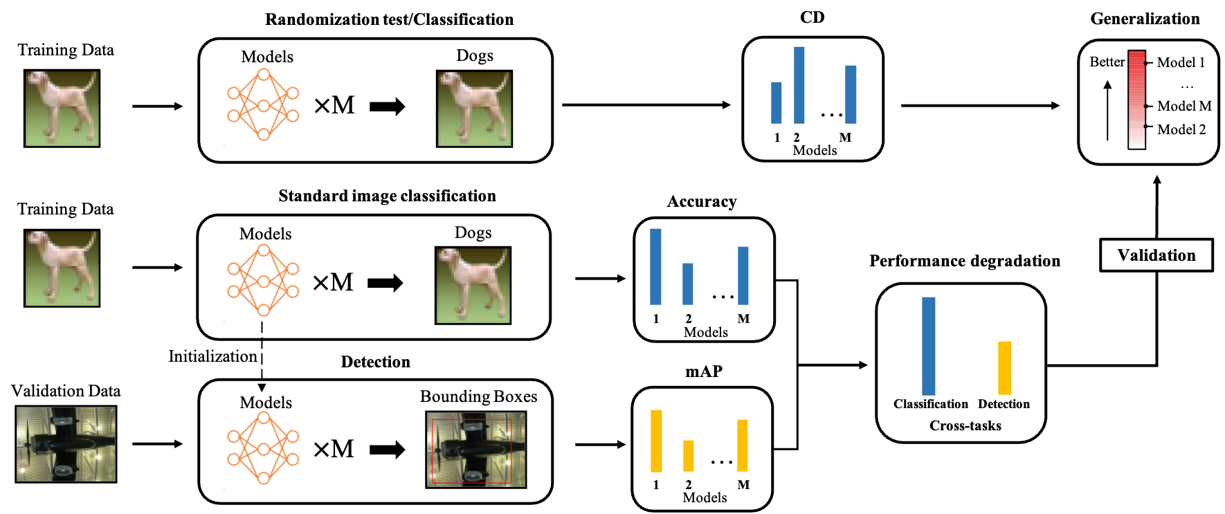
Figure 2: The obtainment and validation of $CD$. Based on the measure of VC-dimension ($p$), training set size, and training error, we calculate the $CD$ of DNNs via a image classification task (Randomization test). Since our proposed $CD$ is a general performance metric regardless of the task, we further validate $CD$ via the cross-tasks (standard image classification and object detection).

Randomization tests: Our methodology is based on a randomization test Zhang et al. (2017). A randomization test is a permutation test based on randomization from non-parametric statistics. We train several candidate architectures on a copy of the data where half of the correct labels are replaced with incorrect labels as described in Eq. 7. For brevity, we define two kinds of labels in our experiments: 1) correct labels: the original labels without modification, 2) incorrect labels: correct labels replaced with incorrect ones.

Dataset: We modify CIFAR-10 Krizhevsky and Hinton (2009) and ImageNet ILSVRC 2012 Deng et al. (2009) for a more straightforward calculation of VC-dimension based on Vapnik and Chervonenkis (1971), which is a fundamental step to calculate the $CD$ of DNNs, then we validate the $CD$ on the PASCAL VOC dataset Everingham et al. (2015) and MS COCO dataset Lin et al. (2014). In order to test the effect of training set size on $CD$, we extract 2,5,7,10 classes from the CIFAR-10 dataset and 2,10,50 classes from the ImageNet dataset. We re-label these datasets with random half incorrect and correct labels as required by the randomization test method.

BNNs: BNNs aim to compress the CNN models by quantizing the weights in the trained CNNs. We are the first to study the generalization ability of BNNs and estimate the performance bound of BNNs. We have selected two commonly used BNNs, PCNN Gu et al. (2019) and ReActNet Liu et al. (2020), in our experiments. We choose PCNN in our experiments because it employs a new BP algorithm in the training process, which can be used to evaluate the generalization ability of different BNNs considering the optimization. ReActNet proposes using RSign and RPReLU to enable explicit learning of the distribution reshape and shift at near-zero extra cost.

4.2 Obtainment: Image Classification

Experimental Setting: We calculate the $CD$ for several commonly used neural networks, including ResNet-18 He et al. (2016), MobileNetV2 Sandler et al. (2018), BNNs (ReActNet and PCNN). The $CD$ is obtained in the image classification task with a SGD optimizer on the CIFAR-10 and ImageNet datasets. In the experiment, we set the learning rate to 0.01, $\alpha=1$ in the Eq. 9, and train the network for 256 epochs. We also show the effect of training set size ($10^{3}$) and training error. We use different numbers of classes in the experiments to explore the effect of various elements on VC-dimension and $CD$. In the section, we will explore the relative generalizations of the different models. The goal is to keep the generalization ranking of different models consistent in different situations. $p$ is calculated based on Eq. 7. As shown in Eq. 8, $p$ is a measure of VC-dimension. We will use the rank of $p$ to represent the rank of VC-dimension.

Table 1: The $CD$ of different models on variants of CIFAR-10 with batch size of 128. A model of a low $CD$ metric indicated by a high rank has a relatively better generalization ability.

#Class	Models	Training set size ($10^{3}$)	Training error	$p$/Rank	$CD$/Rank
2	ReActNet	10	0.512	0.385/4	0.598/4
	PCNN	10	0.371	0.362/3	0.582/3
	ResNet-18	10	0.034	0.102/2	0.413/2
	MobileNetV2	10	0.004	0.022/1	0.355/1
5	ReActNet	25	0.801	0.573/3	0.580/4
	PCNN	25	0.734	0.583/4	0.564/3
	ResNet-18	25	0.056	0.163/2	0.275/2
	MobileNetV2	25	0.001	0.011/1	0.229/1
7	ReActNet	35	0.785	0.638/4	0.698/4
	PCNN	35	0.876	0.634/3	0.696/3
	ResNet-18	35	0.124	0.291/2	0.437/2
	MobileNetV2	35	0.001	0.010/1	0.203/1
10	ReActNet	50	0.900	0.669/4	0.714/4
	PCNN	50	0.792	0.669/3	0.713/3
	ResNet-18	50	0.133	0.300/2	0.423/2
	MobileNetV2	50	0.001	0.006/1	0.272/1

To evaluate the relationship between the generalization ability of BNNs and their full-precision counterparts. We use ResNet-18 as the backbone. To ensure a fair and accurate comparison, we adopt the same experimental setting for different datasets. The $CD$ of ReActNet and PCNN are shown in Tab. 1. We can observe that the $CD$ metric yields a much more stable ranking for these models on various experimental settings, which proves that the $CD$ metric is more stable and reliable than VC-dimension even when the training set size ($10^{3}$) and training error vary. The $CD$ of PCNN is lower than that of ReActNet, indicating that PCNN has better generalization ability. This explains why the performance of the binary network PCNN is better than ReActNet in object detection, even though the pre-trained model of ReActNet is much better performance than PCNN.

To further compare the generalization of the $CD$ metric, we also calculate the $CD$ on ImageNet, and the experimental settings are the same with CIFAR-10. The result is shown in Tab. 2, which reveals full-precision networks always have higher generalization than BNNs. Besides, it can be found that the span of $CD$ is much narrower than that of VC-dimension when using different numbers of classes and training set sizes in Tab. 1 and Tab. 2, which might be a good property of $CD$ metric for DNNs. In the conditions of different numbers of classes and different datasets, the ranking of $CD$ is always consistent though the ranking of VC-dimension is disorder. Even the relationship between errors and $CD$ is not monotonic, $CD$ actually provides a complementary measure based on the training error and VC-dimension. As a result, $CD$ is more stable than VC-dimension.

Table 2: The $CD$ of different models on variants of ImageNet with batch size of 128.

#Class	Models	Training set size ($10^{3}$)	Training error	$p$/Rank	$CD$/Rank
2	ReActNet	2	0.490	0.349/3	0.579/4
	PCNN	2	0.322	0.354/4	0.576/3
	ResNet-18	2	0.281	0.342/2	0.567/2
	MobileNetV2	2	0.378	0.278/1	0.538/1
10	ReActNet	10	0.117	0.645/4	0.688/4
	PCNN	10	0.195	0.642/3	0.687/3
	ResNet-18	10	0.082	0.601/2	0.654/2
	MobileNetV2	10	0.180	0.574/1	0.634/1
50	ReActNet	50	0.133	0.740/4	0.752/4
	PCNN	50	0.087	0.701/3	0.716/3
	ResNet-18	50	0.0347	0.674/2	0.691/2
	MobileNetV2	50	0.333	0.645/1	0.667/1

Table 3: ReActNet with different optimizers on variants of ImageNet with batch size of 128.

#Class	Models	Training set size ($10^{3}$)	Training error	$p$/Rank	$CD$/Rank
2	SGD	2	0.489	0.349/3	0.576/3
	Adam	2	0.190	0.212/1	0.491/2
	AdamW	2	0.013	0.228/2	0.489/1
10	SGD	10	0.117	0.645/3	0.688/3
	Adam	10	0.008	0.328/2	0.441/2
	AdamW	10	0.004	0.299/1	0.418/1
50	SGD	50	0.134	0.740/3	0.752/3
	Adam	50	0.027	0.658/2	0.677/2
	AdamW	50	0.019	0.576/1	0.603/1

We validate the effect of the optimizer for $CD$ in Tab. 3. We can find that the volatility with different optimizers is limited to 44% in $CD$ versus 71% in VC-dimension. Our $CD$ reserves the same ranking for different parameter settings while VC-dimension is inconsistent, which strongly validates that $CD$ can relatively and stably measure the generalization ability of DNNs. In addition, we further validate $CD$ on object detection as a stable metric for the generalization ability measure in Section 4.3.

4.3 Validation: Object Detection

Experimental setting: Our experiments are based on Faster R-CNN Ren et al. (2015) for object detection. We test the performance of Faster RCNN with PCNN and ReActNet (backbone is ResNet-18 or MobilNet V2) in Tab. 4, to validate whether the generalization of them are consistent with the rank of the $CD$ as shown in Tab. 1 and Tab. 2. We first initialize the backbone of Faster RCNN from the pre-trained models, i.e., the models from the image classification task. Note that the convolutions in neck and head of Faster RCNN are also binarized by corresponding method. Then, we use the SGD optimizer with a batch size of 8 and a learning rate of 0.0015, to finetune the networks for 36 epochs.

We evaluate the generalization ability of deep detectors based on the rate of performance change on image classification versus object detection. Since deep detectors are significantly affected by the initially pre-trained models based on image classification, we believe the model with lower rate of performance degradation on object detection than that on image classification achieves better generalization. For example, as shown in Table 4, the model, of larger performance degradation on object classification ($13.2$%) but becoming smaller ($3.9$%) on object detection, gains a better generalization. Through object detection, we reach a safe conclusion that the generalization ranking of the models is consistent with $CD$ in Section 4.2.

Table 4: Test results of BNNs on object detection. The used detection datasets are Pascal VOC and MS COCO. The used classification dataset is ImageNet. ‘W’ and ‘A’ refer to the weight and activation bitwidth, respectively.

Backbone	Binary method	W	A	Accuracy of classification	mAP of detection	Better genera- lized model
VOC2007+ImageNet
ResNet-18	ReAct	1	1	65.9	69.3
ResNet-18	PCNN	1	1	57.2	72.0
Rate of performance change				$13.2\%$ $\downarrow$	$3.9\%$ $\uparrow$	PCNN
VOC2007+ImageNet
ResNet-18	ReAct	1	1	65.9	69.3
MobileNetV2	ReAct	1	1	69.5	74.1
Rate of performance change				5.5% $\uparrow$	6.9% $\uparrow$	MobileNetV2
COCO2017+ImageNet
ResNet-18	ReAct	1	1	65.9	27.5
ResNet-18	PCNN	1	1	57.2	26.9
Rate of performance change				13.2% $\downarrow$	2.2% $\downarrow$	PCNN

The results of ReActNet and PCNN show that even PCNN achieves a much worse performance on the image classification task than ReActNet, it still can achieve close performance (on COCO) or better performance (on VOC) than ReActNet. These results indicate that PCNN trained on the image classification task has a better generalization than ReActNet. We also compare ResNet-18, MobileNetV2 with ReAct. We can see that MobileNetV2 achieves a 5.5% improvement on the image classification task and a 6.9% improvement on the object detection task, which indicates MobileNetV2 performed better on cross-tasks. Conclusively, the generalization of the MobileNetV2 backbone is slightly better than that of the ResNet-18 backbone, which is also in line with the $CD$ ranking. All results demonstrate that the $CD$ is a reliable metric to measure the model’s generalization ability.

5 Conclusion

In this work, we present a flexible framework to understand the capacity and generalization of DNNs. We introduce confidence dimension ($CD$) to measure deep models’ relative generalization ability together with a theoretical analysis, which proves to be the upper bound of the generalization. We validate our $CD$ on cross tasks of object recognition and detection over BNNs and their full-precision counterparts. In future, we will try more applications to validate the effectiveness of our method.

References

- Abelson et al. [1985] Harold Abelson, Gerald Jay Sussman, and Julie Sussman. Structure and Interpretation of Computer Programs. MIT Press, Cambridge, Massachusetts, 1985.
- Arora et al. [2018] Sanjeev Arora, Rong Ge, Behnam Neyshabur, and Yi Zhang. Stronger generalization bounds for deep nets via a compression approach. In International Conference on Machine Learning, pages 254–263. PMLR, 2018.
- Bartlett and Mendelson [2002] Peter L Bartlett and Shahar Mendelson. Rademacher and gaussian complexities: Risk bounds and structural results. The Journal of Machine Learning Research, 3(Nov):463–482, 2002.
- Baumgartner et al. [2001] Robert Baumgartner, Georg Gottlob, and Sergio Flesca. Visual information extraction with Lixto. In Proceedings of the 27th International Conference on Very Large Databases, pages 119–128, Rome, Italy, September 2001. Morgan Kaufmann.
- Bottou [1998] Léon Bottou. Online learning and stochastic approximations. On-Line Learning in Neural Networks, 17(9):142, 1998.
- Bousquet and Elisseeff [2002] Olivier Bousquet and André Elisseeff. Stability and generalization. The Journal of Machine Learning Research, 2:499–526, 2002.
- Brachman and Schmolze [1985] Ronald J. Brachman and James G. Schmolze. An overview of the KL-ONE knowledge representation system. Cognitive Science, 9(2):171–216, April–June 1985.
- Courbariaux et al. [2016] Matthieu Courbariaux, Itay Hubara, Daniel Soudry, Ran El-Yaniv, and Yoshua Bengio. Binarized neural networks: Training deep neural networks with weights and activations constrained to+ 1 or-1. International Conference on Learning Representations, 2016.
- Deng et al. [2009] Jia Deng, Wei Dong, Richard Socher, Li-Jia Li, Kai Li, and Li Fei-Fei. Imagenet: A large-scale hierarchical image database. In Proceedings of the IEEE Conference on Computer Vision and Pattern Recognition, 2009.
- Dinh et al. [2017] Laurent Dinh, Razvan Pascanu, Samy Bengio, and Yoshua Bengio. Sharp minima can generalize for deep nets. In International Conference on Machine Learning, pages 1019–1028. PMLR, 2017.
- Dubhashi and Panconesi [2009] Devdatt P Dubhashi and Alessandro Panconesi. Concentration of measure for the analysis of randomized algorithms. Cambridge University Press, 2009.
- Dziugaite and Roy [2016] Gintare Karolina Dziugaite and Daniel M Roy. Computing nonvacuous generalization bounds for deep (stochastic) neural networks with many more parameters than training data. In Thirty-Third Conference on Uncertainty in Artificial Intelligence, 2016.
- Dziugaite et al. [2020] Gintare Karolina Dziugaite, Alexandre Drouin, Brady Neal, Nitarshan Rajkumar, Ethan Caballero, Linbo Wang, Ioannis Mitliagkas, and Daniel M Roy. In search of robust measures of generalization. In Advances in Neural Information Processing Systems, 2020.
- Everingham et al. [2015] Mark Everingham, SM Ali Eslami, Luc Van Gool, Christopher KI Williams, John Winn, and Andrew Zisserman. The pascal visual object classes challenge: A retrospective. International Journal of Computer Vision, 111(1):98–136, 2015.
- Fort et al. [2019] Stanislav Fort, Paweł Krzysztof Nowak, Stanislaw Jastrzebski, and Srini Narayanan. Stiffness: A new perspective on generalization in neural networks. In International Conference on Learning Representations, 2019.
- Girshick et al. [2014] Ross Girshick, Jeff Donahue, Trevor Darrell, and Jitendra Malik. Rich feature hierarchies for accurate object detection and semantic segmentation. In Proceedings of the IEEE Conference on Computer Vision and Pattern Recognition, 2014.
- Gottlob [1992] Georg Gottlob. Complexity results for nonmonotonic logics. Journal of Logic and Computation, 2(3):397–425, June 1992.
- Gottlob et al. [2002] Georg Gottlob, Nicola Leone, and Francesco Scarcello. Hypertree decompositions and tractable queries. Journal of Computer and System Sciences, 64(3):579–627, May 2002.
- Gu et al. [2019] Jiaxin Gu, Ce Li, Baochang Zhang, Jungong Han, Xianbin Cao, Jianzhuang Liu, and David Doermann. Projection convolutional neural networks for 1-bit cnns via discrete back propagation. In Proceedings of the Association for the Advancement of Artificial Intelligence Conference on Artificial Intelligence, 2019.
- Han et al. [2016] Song Han, Huizi Mao, and William J. Dally. Deep compression: Compressing deep neural networks with pruning, trained quantization and huffman coding. In International Conference on Learning Representations, 2016.
- He et al. [2016] Kaiming He, Xiangyu Zhang, Shaoqing Ren, and Jian Sun. Deep residual learning for image recognition. In Proceedings of the IEEE Conference on Computer Vision and Pattern Recognition, 2016.
- Helwegen et al. [2019] Koen Helwegen, James Widdicombe, Lukas Geiger, Zechun Liu, Kwang-Ting Cheng, and Roeland Nusselder. Latent weights do not exist: Rethinking binarized neural network optimization. In Advances in Neural Information Processing Systems, 2019.
- Hou et al. [2018] Lu Hou, Ruiliang Zhang, and James T Kwok. Analysis of quantized models. In International Conference on Learning Representations, 2018.
- Hubara et al. [2016] Itay Hubara, Matthieu Courbariaux, Daniel Soudry, Ran El-Yaniv, and Yoshua Bengio. Binarized neural networks. In Advances in Neural Information Processing Systems, 2016.
- [25] IJCAI Proceedings. IJCAI camera ready submission. https://proceedings.ijcai.org/info.
- Jiang et al. [2019] Yiding Jiang, Behnam Neyshabur, Hossein Mobahi, Dilip Krishnan, and Samy Bengio. Fantastic generalization measures and where to find them. In International Conference on Learning Representations, 2019.
- Keskar et al. [2017] Nitish Shirish Keskar, Jorge Nocedal, Ping Tak Peter Tang, Dheevatsa Mudigere, and Mikhail Smelyanskiy. On large-batch training for deep learning: Generalization gap and sharp minima. In International Conference on Learning Representations, 2017.
- Kingma and Ba [2015] Diederik P Kingma and Jimmy Ba. Adam: A method for stochastic optimization. In International Conference on Learning Representations, 2015.
- Krizhevsky and Hinton [2009] Alex Krizhevsky and Geoffrey Hinton. Learning multiple layers of features from tiny images. Technical report, University of Toronto, 2009.
- Levesque [1984a] Hector J. Levesque. A logic of implicit and explicit belief. In Proceedings of the Fourth National Conference on Artificial Intelligence, pages 198–202, Austin, Texas, August 1984a. American Association for Artificial Intelligence.
- Levesque [1984b] Hector J. Levesque. Foundations of a functional approach to knowledge representation. Artificial Intelligence, 23(2):155–212, July 1984b.
- Li et al. [2019a] Jian Li, Xuanyuan Luo, and Mingda Qiao. On generalization error bounds of noisy gradient methods for non-convex learning. In International Conference on Learning Representations, 2019a.
- Li et al. [2019b] Rundong Li, Yan Wang, Feng Liang, Hongwei Qin, Junjie Yan, and Rui Fan. Fully quantized network for object detection. In Proceedings of the IEEE Conference on Computer Vision and Pattern Recognition, pages 2810–2819, 2019b.
- Lin et al. [2014] Tsung-Yi Lin, Michael Maire, Serge Belongie, James Hays, Pietro Perona, Deva Ramanan, Piotr Dollár, and C Lawrence Zitnick. Microsoft coco: Common objects in context. In Proceedings of the European Conference on Computer Vision, 2014.
- Liu et al. [2019] Jinlong Liu, Yunzhi Bai, Guoqing Jiang, Ting Chen, and Huayan Wang. Understanding why neural networks generalize well through gsnr of parameters. In International Conference on Learning Representations (ICLR), 2019.
- Liu et al. [2018] Zechun Liu, Baoyuan Wu, Wenhan Luo, Xin Yang, Wei Liu, and Kwang-Ting Cheng. Bi-real net: Enhancing the performance of 1-bit cnns with improved representational capability and advanced training algorithm. In Proceedings of the European Conference on Computer Vision, 2018.
- Liu et al. [2020] Zechun Liu, Zhiqiang Shen, Marios Savvides, and Kwang-Ting Cheng. Reactnet: Towards precise binary neural network with generalized activation functions. In Proceedings of the European Conference on Computer Vision, 2020.
- Loshchilov and Hutter [2018] Ilya Loshchilov and Frank Hutter. Fixing weight decay regularization in adam. In International Conference on Learning Representations, 2018.
- Mukherjee et al. [2004] Sayan Mukherjee, Partha Niyogi, Tomaso Poggio, and Ryan Rifkin. Statistical learning: Stability is sufficient for generalization and necessary and sufficient for consistency of empirical risk minimization. Technical report, 2004.
- Nagarajan and Kolter [2019] Vaishnavh Nagarajan and J Zico Kolter. Uniform convergence may be unable to explain generalization in deep learning. In Advances in Neural Information Processing Systems, 2019.
- Nebel [2000] Bernhard Nebel. On the compilability and expressive power of propositional planning formalisms. Journal of Artificial Intelligence Research, 12:271–315, 2000.
- Neyshabur et al. [2017] Behnam Neyshabur, Srinadh Bhojanapalli, David McAllester, and Nathan Srebro. Exploring generalization in deep learning. In Advances in Neural Information Processing Systems, 2017.
- Neyshabur et al. [2019] Behnam Neyshabur, Zhiyuan Li, Srinadh Bhojanapalli, Yann LeCun, and Nathan Srebro. Towards understanding the role of over-parametrization in generalization of neural networks. In International Conference on Learning Representations, 2019.
- Poggio et al. [2004] Tomaso Poggio, Ryan Rifkin, Sayan Mukherjee, and Partha Niyogi. General conditions for predictivity in learning theory. Nature, 428(6981):419–422, 2004.
- Rastegari et al. [2016] Mohammad Rastegari, Vicente Ordonez, Joseph Redmon, and Ali Farhadi. Xnor-net: Imagenet classification using binary convolutional neural networks. In Proceedings of the European Conference on Computer Vision, 2016.
- Ren et al. [2015] Shaoqing Ren, Kaiming He, Ross B Girshick, and Jian Sun. Faster r-cnn: Towards real-time object detection with region proposal networks. In Advances in Neural Information Processing Systems, 2015.
- Sandler et al. [2018] Mark Sandler, Andrew Howard, Menglong Zhu, Andrey Zhmoginov, and Liang-Chieh Chen. Mobilenetv2: Inverted residuals and linear bottlenecks. In Proceedings of the IEEE conference on computer vision and pattern recognition, 2018.
- Srivastava et al. [2014] Nitish Srivastava, Geoffrey Hinton, Alex Krizhevsky, Ilya Sutskever, and Ruslan Salakhutdinov. Dropout: a simple way to prevent neural networks from overfitting. The Journal of Machine Learning Research, 15(1):1929–1958, 2014.
- Sun et al. [2016] Shizhao Sun, Wei Chen, Liwei Wang, Xiaoguang Liu, and Tie-Yan Liu. On the depth of deep neural networks: A theoretical view. In Proceedings of the Association for the Advance of Artificial Intelligence Conference on Artificial Intelligence, 2016.
- Valle-Pérez and Louis [2020] Guillermo Valle-Pérez and Ard A Louis. Generalization bounds for deep learning. In International Conference on Learning Representations, 2020.
- Valle-Perez et al. [2018] Guillermo Valle-Perez, Chico Q Camargo, and Ard A Louis. Deep learning generalizes because the parameter-function map is biased towards simple functions. In International Conference on Learning Representations, 2018.
- Vapnik and Chervonenkis [1971] VN Vapnik and A Ya Chervonenkis. On the uniform convergence of relative frequencies of events to their probabilities. Measures of Complexity, 16(2):11, 1971.
- Wu et al. [2018] Shuang Wu, Guoqi Li, Feng Chen, and Luping Shi. Training and inference with integers in deep neural networks. In International Conference on Learning Representations, 2018.
- Yin et al. [2019] P Yin, J Lyu, S Zhang, S Osher, YY Qi, and J Xin. Understanding straight-through estimator in training activation quantized neural nets. In International Conference on Learning Representations, 2019.
- Zhang et al. [2017] Chiyuan Zhang, Samy Bengio, Moritz Hardt, Benjamin Recht, and Oriol Vinyals. Understanding deep learning requires rethinking generalization. In International Conference for Learning Representations, 2017.
- Zhou et al. [2017] Yanzhao Zhou, Qixiang Ye, Qiang Qiu, and Jianbin Jiao. Oriented response networks. In IEEE Conference on Computer Vision and Pattern Recognition, 2017.
- Zoph and Le [2016] B. Zoph and Q. V. Le. Neural architecture search with reinforcement learning. In International Conference on Learning Representations, 2016.