Experimental Quantum End-to-End Learning on a Superconducting Processor

Abstract

Machine learning can be substantially powered by a quantum computer owing to its huge Hilbert space and inherent quantum parallelism. In the pursuit of quantum advantages for machine learning with noisy intermediate-scale quantum devices, it was proposed that the learning model can be designed in an end-to-end fashion, i.e., the quantum ansatz is parameterized by directly manipulable control pulses without circuit design and compilation. Such gate-free models are hardware friendly and can fully exploit limited quantum resources. Here, we report the first experimental realization of quantum end-to-end machine learning on a superconducting processor. The trained model can achieve $98\%$ recognition accuracy for two handwritten digits (via two qubits) and $89\%$ for four digits (via three qubits) in the MNIST (Mixed National Institute of Standards and Technology) database. The experimental results exhibit the great potential of quantum end-to-end learning for resolving complex real-world tasks when more qubits are available.

Quantum computing Nielsen and Chuang (2000) is revolutionizing the field of machine learning (ML) Biamonte et al. (2017); Dunjko and Briegel (2018); Sarma et al. (2019). Powered by quantum Fourier transform and amplitude amplification, provable speed-up has been predicted for high-dimensional and big-data ML tasks using fault-tolerant quantum computers Lloyd et al. (2014); Rebentrost et al. (2014); Amin et al. (2018); Dunjko et al. (2016); Gao et al. (2018). Even with noisy intermediate-scale quantum (NISQ) devices, quantum advantage is still promising, because the model expressibility can be substantially enhanced by the exponentially large feature space carried by multi-qubit quantum states Liu et al. (2021); Schuld and Killoran (2019).

To deploy quantum machine learning algorithms on NISQ processors, the key part is to construct a parameterized quantum ansatz that can be trained by a classical optimizer. To date, most quantum ansatzes are realized by quantum neural networks (QNN) Havlíček et al. (2019); Liu et al. (2021); Benedetti et al. (2019); Schuld et al. (2020); Farhi and Neven (2018); Wei et al. (2022); Houssein et al. (2022); Farhi et al. (2014); Wurtz and Lykov (2021); Rudolph et al. ; Zeng et al. (2019); Jerbi et al. (2021) that consist of layers of parameterized quantum gates, and successful experiments have been demonstrated on classification Tacchino et al. (2019); Cai et al. (2015); Johri et al. (2021), clustering Ouyang et al. (2020); Li et al. (2015), and generative Zoufal et al. (2019); Hu et al. (2019); Zhu et al. (2019) learning tasks. The gate-based QNN ansatz naturally incorporates the theory of quantum circuits, but the learning performance is highly dependent on the architecture design and the mapping of circuits to experimentally operable native gates. A structurally non-optimized QNN cannot fully exploit the limited quantum coherence resource, and this is partially why high learning accuracy is hard to attain on NISQ devices without downsizing the training dataset.

There are certainly much room for performance improvement by using more hardware-efficient quantum ansatzes, e.g., via deep optimization of the circuit architecture Ostaszewski et al. (2021) and qubit mapping strategies Huang et al. (2021). Recently, a hardware-friendly end-to-end learning scheme (in the sense that the model is trained as a whole instead of being divided into separate modules) is proposed Wu et al. (2020) by replacing the gate-based QNN with natural quantum dynamics driven by coherent control pulses. This model requires very little architecture design, system calibration, and no qubit mapping. One can also jointly train a data encoder that automatically transforms classical data to quantum states via control pulses, and this essentially simplifies the encoding process because the preparation of quantum states according to a hand-designed encoding scheme is no more required. More importantly, the natural control-to-state mapping involved in the encoding process introduces nonlinearity that is crucial for better model expressibility.

In this paper, we report the first experimental demonstration of quantum end-to-end machine learning using a superconducting processor through the recognition of handwritten digits selected from the MNIST (Mixed National Institute of Standards and Technology) dataset. Without downsizing the original 784-pixel images, the end-to-end learning model can be trained to achieve $98\%$ accuracy with two qubits for the 2-digit classification and $89\%$ accuracy with three qubits for the 4-digit task, which are among the best experimental results reported on small-size quantum processors Wang et al. (2021). The demonstrated quantum end-to-end model can be easily scaled up for solving complex real-world learning tasks owing to its inherent hardware friendliness and efficiency.

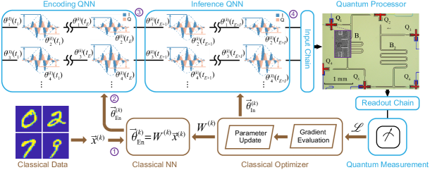
Figure 1: (Color online) The training protocol of the quantum end-to-end learning framework. In the $k$-th iteration, a randomly selected image of a handwritten digit in the MNIST dataset is converted to a vector $\vec{x}^{(k)}$ and then transformed by a matrix $W^{(k)}$ to the control variables $\vec{\theta}^{(k)}_{\mathrm{En}}$ that steer the quantum state to $\left|\psi^{(k)}(t_{E})\right\rangle$ of the qubits in the QNN. This process encodes $\vec{x}^{(k)}$ to $\left|\psi^{(k)}\right\rangle$. Subsequent inference control pulses $\vec{\theta}^{(k)}_{\mathrm{In}}$ are applied to drive $\left|\psi^{(k)}(t_{E})\right\rangle$ to $\left|\psi^{(k)}(t_{E+I})\right\rangle$ that is to be measured. The parameters in $W^{(k)}$ and $\vec{\theta}^{(k)}_{\mathrm{In}}$ are updated for the next iteration according to the loss function $\mathcal{L}$ and its gradient obtained from the measurement. The circled numbers represent the specific points in the data flow and the corresponding learning performances are shown in Fig. 4. The top right is the false-colored optical image of the six-qubit device used in our experiment.

The basic idea of end-to-end quantum learning is to parameterize the quantum ansatz by physical control pulses that are usually applied to implement abstract quantum gates in variational quantum classifiers. In this way, a feedforward QNN can be constructed by the control-driven evolution of the quantum state $\left|\psi(t)\right\rangle$, as follows Rivas and Huelga (2012):

$$\frac{d\left|\psi(t)\right\rangle}{dt}=-\frac{i}{\hbar}\left[H_{0}+\sum_{m=1}^{r}\theta_{m}(t)H_{m}\right]\left|\psi(t)\right\rangle,$$ (1)

where $H_{0}$ is the static Hamiltonian which involves the coupling between different qubits, and $r$ is the number of pulsed control functions/channels in the quantum processor. For example, if there are $M$ qubits for the QNN and each qubit is dictated by $c$ control functions (e.g., flux bias or microwave driving), we have $r=c\times M$. Here, $H_{m}$ is the control Hamiltonian associated with the $m$-th control pulse that contains $n$ sub-pulses over $n$ sampling periods. The $j$-th sub-pulse is parameterized by $\theta_{m}(t_{j})$, and hence we denote the $m$-th control pulse by $\vec{\theta}_{m}=[{\theta}_{m}(t_{1}),{\theta}_{m}(t_{2}),...,{\theta}_{m}(t_{n})]$. The evolution of the quantum system under all $n$-th control sub-pulses constructs the $n$-th layer of the QNN.

We illustrate the quantum end-to-end learning with a classification task based on the MNIST dataset. As shown in Fig. 1, an image of a handwritten digit is randomly selected from the training dataset $\mathcal{D}$. In the $k$-th iteration, the sampled image is converted to a $d=784$ dimensional vector $\vec{x}^{(k)}$, and $y^{(k)}$ is the corresponding label. The input data $\vec{x}^{(k)}$ is transformed by a matrix $W^{(k)}$ to the control variables $\vec{\theta}^{(k)}_{\mathrm{En}}=W^{(k)}\vec{x}^{(k)}$. This constructs a classical encoding block with $r$ channels and $E$ sub-pulses per channel: $\vec{\theta}^{(k)}_{\mathrm{En}}=[{\theta}^{(k)}_{1}(t_{1}),...,{\theta}^{(k)}_{1}(t_{\mathrm{E}}),...,{\theta}^{(k)}_{r}(t_{1})...,{\theta}^{(k)}_{r}(t_{E})]$. The generated control pulses $\vec{\theta}^{(k)}_{\mathrm{En}}$ then automatically encode $\vec{x}^{(k)}$ to the quantum state $\left|\psi^{(k)}(t_{E})\right\rangle$ via the natural quantum state evolution of Eq. (1).

Subsequent inference control pulses $\vec{\theta}^{(k)}_{\mathrm{In}}$, which have the same form as $\vec{\theta}^{(k)}_{\mathrm{En}}$ but consist of $I$ sub-pulses in each channel, are then applied to induce the quantum evolution from the encoded quantum state $\left|\psi^{(k)}(t_{E})\right\rangle$. The inference controls are introduced for improving the classification performance. Finally, the end-time quantum state $\left|\psi^{(k)}(t_{E+I})\right\rangle$ is measured under the appropriate experiment-available positive operator $O^{(k)}$ according to the classical label $y^{(k)}$, which gives the conditional probability (or confidence) of obtaining $y^{(k)}$ for a given input $\vec{x}^{(k)}$

$$P(y^{(k)}|\vec{x}^{(k)},W^{(k)},\vec{\theta}^{(k)}_{\mathrm{{In}}})=\left\langle\psi^{(k)}(t_{E+I})\right|O^{(k)}\left|\psi^{(k)}(t_{E+I})\right\rangle.$$ (2)

The corresponding loss function is defined as

$$\mathcal{L}[W^{(k)},\vec{\theta}^{(k)}_{\mathrm{In}},\{\vec{x}_{\ell}^{(k)}\}]=1-\frac{1}{b}\sum_{\ell=1}^{b}P(y^{(k)}|\vec{x}_{\ell}^{(k)},W^{(k)},\vec{\theta}^{(k)}_{\mathrm{{In}}}).$$ (3)

In the experiment, we select a batch of $b$ samples in each iteration to reduce the fluctuation of $\mathcal{L}$ for faster convergence of the learning process. The gradient of the loss function $\mathcal{L}$ with respect to the encoding control $\vec{\theta}^{(k)}_{\mathrm{En}}$ and the inference control $\vec{\theta}^{(k)}_{\mathrm{In}}$ can be evaluated with the finite difference method by making a small change of the each control parameter $\theta^{(k)}_{i}(t_{j})$ Li (2005). The gradient of $\mathcal{L}$ with respect to $W^{(k)}$ can be derived from the gradient of $\mathcal{L}$ with respect to $\vec{\theta}^{(k)}_{\mathrm{En}}$ Wu et al. (2020). Therefore, we can apply the widely used stochastic gradient-descent algorithm in machine learning to update $W^{(k)}$ and $\vec{\theta}^{(k)}_{\mathrm{In}}$ by minimizing $\mathcal{L}$ on the training dataset $\mathcal{D}$ (see Supplementary Materials for details of the algorithms) Friedman (2002). Once the model is well trained, one can use fresh samples from a testing dataset to examine the recognition performance of the handwritten digits.

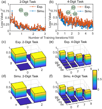
Figure 2: (Color online) (a) and (b) The typical training process of the end-to-end model. For better clarity, all data points are averaged over the neighboring four points. (c-f) The classification performance of the trained model. The horizontal labels show the digits to be classified, while the vertical labels show the majority vote of the computational basis measurement results. (c) and (d) Experimental and simulation results for the 2-digit classification task, respectively. The averaged accuracies for the classification are $0.987$ and $0.982$ in the experiment and the simulation, respectively. (e) and (f) The 4-digit classification of the QNN. The averaged accuracies are 0.895 and 0.889 in the experiment and the simulation, respectively.

The end-to-end model is demonstrated in a superconducting processor, as shown in Fig. 1. All qubits take the form of the flux-tunable Xmon geometry and are driven with inductively coupled flux bias lines and capacitively coupled RF control lines Barends et al. (2013); Li et al. (2018); Cai et al. (2019). Among the six qubits, $Q_{1},Q_{2},Q_{4},Q_{5}$ are dispersively coupled to a half-wavelength coplanar cavity $B_{1}$, and $Q_{2},Q_{3},Q_{5},Q_{6}$ are dispersively coupled to another cavity $B_{2}$. Each qubit is dispersively coupled to a quarter-wavelength readout resonator for a high-fidelity single-shot readout and all the resonators are coupled to a common transmission line for multiplexed readouts. The qubits that are not relevant to the QNN is biased far away and can be ignored from the system Hamiltonian, therefore, the static Hamiltonian of the QNN can be written in the interaction picture as

$$H_{0}/\hbar=\sum_{q\neq{p}}J_{qp}(a_{q}^{\dagger}{}a_{p}+a_{p}^{\dagger}{}a_{q})-\sum_{q=1}^{M}{}\frac{E_{C,q}}{2}a_{q}^{\dagger}{}a_{q}^{\dagger}{}a_{q}a_{q},$$ (4)

where $J_{qp}$ is the coupling strength between the $p$-th and $q$-th qubits mediated by the bus cavity, $E_{C,q}$ denotes the qubit anharmonicity, and $a_{q}$ is the annihilation operator of the $q$-th qubit.

Throughout this work, we set the encoding block with $E=2$ layers followed by an inference block with $I=2$ layers. As shown in Fig. 1, for the $q$-th qubit in the $n$-th ($n=1,2,3,4$) layer of the QNN, there are $c=2$ control parameters $\theta_{2q-1}(t_{n})$ and $\theta_{2q}(t_{n})$, which are associated with the control Hamiltonians $H_{2q-1}=(a_{q}+a_{q}^{\dagger})/2$ (rotation along the $x$-axis of the Bloch sphere) and $\quad H_{2q}=(ia_{q}-ia_{q}^{\dagger})/2$ (rotation along the $y$-axis of the Bloch sphere), respectively. The control parameters are the variable amplitudes of the Gaussian envelopes of two resonant microwave sub-pulses, each of which has a fixed width of $4\sigma=40$ ns. All the quantum controls in the same time interval are exerted simultaneously. For an $N$-digit classification task, we take $M=\lceil\log_{2}{N}\rceil+1$ qubits for the QNN: the classification results are mapped to the computation bases of the first $\lceil\log_{2}{N}\rceil$ qubits (label qubits) by the majority vote of the collective measurement performed on label qubits, while one additional qubit is introduced for a better expressibility of the model. Therefore, the QNN in our experiment involves totally $cM(E+I)=8M$ control parameters.

We perform the 2-digit (‘0’ and ‘2’) classification task ($N=2$) with $Q_{3}$ and $Q_{5}$ ($M=2$). The working frequencies are $6.08$ GHz and $6.45$ GHz, respectively, which are also the flux sweet-spots of the two qubits. The effective coupling strength $J_{35}/2\pi=4.11$ MHz. We take $Q_{5}$ as the label qubit and assign the classification result to be ‘0’ or ‘2’ if the respective probability of measuring $\left|g\right\rangle$ or $\left|e\right\rangle$ state is larger.

The end-to-end model is initialized with $W=W_{0}$ and $\vec{\theta}_{\mathrm{In}}=\vec{\theta}_{0}$, where all elements of $W_{0}$ are $10^{-5}$ and each element of $\vec{\theta}_{0}$ is tuned to induce a $\pi/4$ rotation of the respective qubit. The parameter update is realized as follows. Firstly, we obtain the loss function $\mathcal{L}$ according to Eq. (3) by measuring $Q_{5}$. We perturb each control parameter in the control set $\{\vec{\theta}_{\mathrm{En}},\vec{\theta}_{\mathrm{In}}\}$ and obtain the corresponding gradient of $\mathcal{L}$. The $\mathcal{L}$ and its gradient averaged over a batch of two training samples ($b=2$) are sent to a classical Adam optimizer Kingma and Ba (2015) for updating $W$ and $\vec{\theta}_{\mathrm{In}}$. All control parameters are linearly scaled to the digital-to-analog converter level of a Tektronix arbitrary waveform generator 70002A, working with a sampling rate of $25$ GHz, to generate the resonant RF pulses directly. The control pulses composed of in-phase and quadrature components are sent to each qubit with the corresponding RF control line. To obtain the classification result, we repeat the procedure and measure the label qubit for $5000$ times.

In the 4-digit (’0’, ’2’, ’7’, and ’9’) classification task ($N=4$), we take $Q_{3}$, $Q_{5}$, and $Q_{6}$ ($M=3$) to construct the QNN, whose working frequencies are 6.08 GHz, 6.45 GHz, and 6.19 GHz, respectively. $Q_{3}$ and $Q_{5}$ are measured for the classification output. The target digits correspond to the four computational bases spanned by the two label qubits. The training procedure and algorithms are the same as those for the $N=2$ task.

The typical training process is shown in Figs. 2a-b. For better clarity, the curves are smoothed out by averaging each data point from its neighboring four ones. For the 2-digit (4-digit) classification task, the experimental loss function $\mathcal{L}$ converges to 0.14 (0.22) in 300 (500) iterations. The training loss can potentially be reduced by increasing the depth $E$ of the encoding block Wu et al. (2020). For comparison, numerical simulations are also performed with the calibrated system Hamiltonian, the same batches of training samples, and the same parameter update algorithms. As shown in Figs. 2a-b, the simulations match the experiments well. The small deviation of the experimental data may attribute to the simplified modeling of high-order couplings between the qubits and the control pulses Motzoi et al. (2009), as well as the system parameter drifting.

To examine the performance of the end-to-end learning, we experimentally test the generalizability of the trained end-to-end model with fresh testing samples (1000 for each digit), and count the frequencies of assigning these samples to different digits (see Figs. 2c-f). The measured overall accuracies (i.e., the proportion of samples that are correctly classified) are $98.7\%$ for the 2-digit task and $89.5\%$ for the 4-digit task, respectively, which are consistent with the simulation results ($98.2\%$ and $88.9\%$, respectively) based on the experimentally identified Hamiltonian.

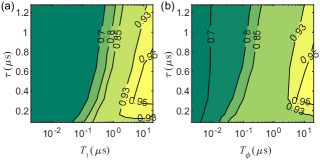
Figure 3: (a) The simulated average confidence as a function of the qubit relaxation time $T_{1}$ and the pulse length $\tau$, while the qubit pure dephasing time $T_{\phi}$ is infinite; (b) The simulated average confidence as a function of $T_{\phi}$ and $\tau$, while $T_{1}$ is infinite.

The performance of the model also relies on the amount of entanglement gained in the quantum state. When the number of QNN layers is fixed, the quantum state gets more entangled under longer pulse length $\tau$ (includes all the $E+I=4$ sub-pulses in both the encoding and the inference blocks), but coherence may be lost in the prolonged control time duration due to the inevitable decoherence. We use the experimentally calibrated parameters to simulate the 2-digit classification process under different $\tau$ and different coherence times $T_{1}$ and $T_{\phi}$ of the qubits. As shown in Fig. 3, the average confidence $1-\mathcal{L}$ varies little with $\tau$ when $T_{1}$ or $T_{\phi}$ is sufficiently small because the coherent control is overwhelmed by the strong decoherence. For larger $T_{1}$ or $T_{\phi}$ (e.g., $T_{1}=20~{}\mu$s), the average confidence initially increases with $\tau$, but then decreases after reaching the peak. This trend clearly indicates the trade-off between the gained entanglement and the lost coherence, and thus $\tau$ as well as the number of layers should be optimally chosen for the best balance.

The end-to-end learning scheme provides a seamless combination of quantum and classical computers through the joint training of the control-based QNN and the classical data encoder $W$. To understand their respective roles in the classification, we check how the data distribution varies along the flow $\vec{x}\rightarrow\vec{\theta}_{\mathrm{En}}\rightarrow\left|\psi(t_{E})\right\rangle\rightarrow\left|\psi(t_{E+I})\right\rangle\rightarrow y$ (see $①\sim④$ in Fig. 1) in the 2-digit classification process. To facilitate the analysis, we use the Linear Discriminant Analysis (LDA) Venables and Ripley (2013) that projects high-dimensional data vectors into two clusters of points distributed on an optimally chosen line (see details in the Supplementary Materials). The LDA makes it easier to visualize and compare data distributions whose dimensionalities are different.

The projected clusters are plotted in Fig. 4. In each sub-figure, the distance between the centers of the two clusters is normalized, and hence we can quantify the classifiability by their standard deviations (i.e., the narrowness of distribution). As can be seen in Figs. 4a-b, the classical data encoder $W$ effectively reduces the original 784-dimensional vector $\vec{x}$ to a 8-dimensional vector of control variables $\vec{\theta}_{\mathrm{En}}$, but the standard deviation is increased from $0.1658$ for the original dataset to $0.2903$ for the transformed control pulses. Then, the control-to-state mapping, which is both nonlinear and quantum, sharply reduces the standard deviation to $0.0919$ for the encoded quantum state (Fig. 4c), while the following quantum inference block does not make further improvement (Fig. 4d). These results indicate that the classical data encoder is responsible for the compression of the high-dimensional input data, while the classification is mainly accomplished by the QNN.

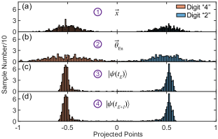
Figure 4: The projected points by using LDA, where the distance between the projected cluster centers is normalized. The positions of $①\sim④$ along the data flow are shown in Fig. 1. (a) The projected points of the original 784-dimensional handwritten digits. (b) The projected points of the control pulses for encoding the classical data to the quantum states. (c) The projected points of the quantum states after the encoding block. (d) The projected points of the final quantum states.

It should be noted that no quantum advantage is claimed here with a small-size NISQ processor. However, we notice that the end-to-end learning is very similar to quantum reservoir computing (QRC) Mujal et al. (2021); Ghosh et al. (2019) in that both schemes exploit complex natural quantum dynamics for hard computing tasks, and QRC has been proven to have universal approximation property Chen et al. (2020) and higher information processing capacity Bravo et al. (2021). It is conjectured that similar conclusions can be made for quantum end-to-end learning, and these will be explored in our future studies.

Apparently, the power of QNN can be exponentially increased when more controllable qubits are available. We expect to further improve the training efficiency of the end-to-end learnings on larger NISQ processors, and develop more complicated ML application (e.g., unsupervised and generative learning) based on more complex datasets.

This work was supported by National Key Research and Development Program of China (Grants No. 2017YFA0304303 and 2017YFA0304304), the National Natural Science Foundation of China (Grants No. 92165209, No. 61833010, No. 62173201, No. 11925404, No. 11874235, No. 11874342, No. 11922411, No. 12061131011, No. 12075128), Key-Area Research and Development Program of Guangdong Provice (Grant No. 2020B0303030001), Anhui Initiative in Quantum Information Technologies (AHY130200), China Postdoctoral Science Foundation (BX2021167), and Grant No. 2019GQG1024 from the Institute for Guo Qiang, Tsinghua University. D.-L. D. also acknowledges additional support from the Shanghai Qi Zhi Institute.

References

- Nielsen and Chuang (2000) M. A. Nielsen and I. L. Chuang, Quantum Computation and Quantum Information (Cambridge Univ. Press, 2000).
- Biamonte et al. (2017) J. Biamonte, P. Wittek, N. Pancotti, P. Rebentrost, N. Wiebe, and S. Lloyd, “Quantum machine learning,” Nature 549, 195 (2017).
- Dunjko and Briegel (2018) V. Dunjko and H. J. Briegel, “Machine learning & artificial intelligence in the quantum domain: a review of recent progress,” Rep. Prog. Phys. 81, 074001 (2018).
- Sarma et al. (2019) S. D. Sarma, D.-L. Deng, and L. Duan, “Machine learning meets quantum physics,” Phys. Today 72, 48 (2019).
- Lloyd et al. (2014) S. Lloyd, M. Mohseni, and P. Rebentrost, “Quantum principal component analysis,” Nat. Phys. 10, 631 (2014).
- Rebentrost et al. (2014) P. Rebentrost, M. Mohseni, and S. Lloyd, “Quantum support vector machine for big data classification,” Phys. Rev. Lett. 113, 130503 (2014).
- Amin et al. (2018) M. H. Amin, E. Andriyash, J. Rolfe, B. Kulchytskyy, and R. Melko, “Quantum boltzmann machine,” Phys. Rev. X 8, 021050 (2018).
- Dunjko et al. (2016) V. Dunjko, J. M. Taylor, and H. J. Briegel, “Quantum-enhanced machine learning,” Phys. Rev. Lett. 117, 130501 (2016).
- Gao et al. (2018) X. Gao, Z.-Y. Zhang, and L.-M. Duan, “A quantum machine learning algorithm based on generative models,” Sci. Adv. 4, eaat9004 (2018).
- Liu et al. (2021) Y. Liu, S. Arunachalam, and K. Temme, “A rigorous and robust quantum speed-up in supervised machine learning,” Nat. Phys. 17, 1013 (2021).
- Schuld and Killoran (2019) M. Schuld and N. Killoran, “Quantum machine learning in feature hilbert spaces,” Phys. Rev. Lett. 122, 040504 (2019).
- Havlíček et al. (2019) V. Havlíček, A. D. Córcoles, K. Temme, A. W. Harrow, A. Kandala, J. M. Chow, and J. M. Gambetta, “Supervised learning with quantum-enhanced feature spaces,” Nature 567, 209 (2019).
- Benedetti et al. (2019) M. Benedetti, E. Lloyd, S. Sack, and M. Fiorentini, “Parameterized quantum circuits as machine learning models,” Quantum Sci. Technol. 4, 043001 (2019).
- Schuld et al. (2020) M. Schuld, A. Bocharov, K. M. Svore, and N. Wiebe, “Circuit-centric quantum classifiers,” Phys. Rev. A 101, 032308 (2020).
- Farhi and Neven (2018) E. Farhi and H. Neven, “Classification with quantum neural networks on near term processors,” arXiv:1802.06002 (2018).
- Wei et al. (2022) S. Wei, Y. Chen, Z. rong Zhou, and G. Long, “A quantum convolutional neural network on nisq devices,” AAPPS Bull. (2022).
- Houssein et al. (2022) E. H. Houssein, Z. Abohashima, M. Elhoseny, and W. M. Mohamed, “Hybrid quantum-classical convolutional neural network model for COVID-19 prediction using chest X-ray images,” J. Comput. Des. Eng. 9, 343 (2022).
- Farhi et al. (2014) E. Farhi, J. Goldstone, and S. Gutmann, “A quantum approximate optimization algorithm,” arXiv:1411.4028 (2014).
- Wurtz and Lykov (2021) J. Wurtz and D. Lykov, “Fixed-angle conjectures for the quantum approximate optimization algorithm on regular maxcut graphs,” Phys. Rev. A 104, 052419 (2021).
- (20) M. S. Rudolph, N. B. Toussaint, A. Katabarwa, S. Johri, B. Peropadre, and A. Perdomo-Ortiz, “Generation of high-resolution handwritten digits with an ion-trap quantum computer,” arXiv:2012.03924 .
- Zeng et al. (2019) J. Zeng, Y. Wu, J.-G. Liu, L. Wang, and J. Hu, “Learning and inference on generative adversarial quantum circuits,” Phys. Rev. A 99, 052306 (2019).
- Jerbi et al. (2021) S. Jerbi, C. Gyurik, S. Marshall, H. Briegel, and V. Dunjko, “Parametrized quantum policies for reinforcement learning,” NIPS 34 (2021).
- Tacchino et al. (2019) F. Tacchino, C. Macchiavello, D. Gerace, and D. Bajoni, “An artificial neuron implemented on an actual quantum processor,” npj Quantum Inform. 5, 1 (2019).
- Cai et al. (2015) X.-D. Cai, D. Wu, Z.-E. Su, M.-C. Chen, X.-L. Wang, L. Li, N.-L. Liu, C.-Y. Lu, and J.-W. Pan, “Entanglement-based machine learning on a quantum computer,” Phys. Rev. Lett. 114, 110504 (2015).
- Johri et al. (2021) S. Johri, S. Debnath, A. Mocherla, A. Singk, A. Prakash, J. Kim, and I. Kerenidis, “Nearest centroid classification on a trapped ion quantum computer,” npj Quantum Inform. 7, 1 (2021).
- Ouyang et al. (2020) X.-L. Ouyang, X.-Z. Huang, Y.-K. Wu, W.-G. Zhang, X. Wang, H.-L. Zhang, L. He, X.-Y. Chang, and L.-M. Duan, “Experimental demonstration of quantum-enhanced machine learning in a nitrogen-vacancy-center system,” Phys. Rev. A 101, 012307 (2020).
- Li et al. (2015) Z. Li, X. Liu, N. Xu, and J. Du, “Experimental realization of a quantum support vector machine,” Phys. Rev. Lett. 114, 140504 (2015).
- Zoufal et al. (2019) C. Zoufal, A. Lucchi, and S. Woerner, “Quantum generative adversarial networks for learning and loading random distributions,” npj Quantum Inform. 5, 1 (2019).
- Hu et al. (2019) L. Hu, S.-H. Wu, W. Cai, Y. Ma, X. Mu, Y. Xu, H. Wang, Y. Song, D.-L. Deng, C.-L. Zou, et al., “Quantum generative adversarial learning in a superconducting quantum circuit,” Sci. Adv. 5, eaav2761 (2019).
- Zhu et al. (2019) D. Zhu, N. M. Linke, M. Benedetti, K. A. Landsman, N. H. Nguyen, C. H. Alderete, A. Perdomo-Ortiz, N. Korda, A. Garfoot, C. Brecque, et al., “Training of quantum circuits on a hybrid quantum computer,” Sci. Adv. 5, eaaw9918 (2019).
- Ostaszewski et al. (2021) M. Ostaszewski, L. Trenkwalder, W. Masarczyk, E. Scerri, and V. Dunjko, “Reinforcement learning for optimization of variational quantum circuit architectures,” NIPS 34 (2021).
- Huang et al. (2021) H.-Y. Huang, M. Broughton, M. Mohseni, R. Babbush, S. Boixo, H. Neven, and J. R. McClean, “Power of data in quantum machine learning,” Nat. Commun. 12 (2021).
- Wu et al. (2020) R.-B. Wu, X. Cao, P. Xie, and Y.-x. Liu, “End-To-End Quantum Machine Learning Implemented with Controlled Quantum Dynamics,” Phys. Rev. Appl. 14, 064020 (2020).
- Wang et al. (2021) K. Wang, L. Xiao, W. Yi, S.-J. Ran, and P. Xue, “Experimental realization of a quantum image classifier via tensor-network-based machine learning,” Photonics Res. (2021).
- Rivas and Huelga (2012) A. Rivas and S. F. Huelga, Open quantum systems, Vol. 10 (Springer, 2012).
- Li (2005) J. Li, “General explicit difference formulas for numerical differentiation,” J. Comput. Appl. Math. 183, 29 (2005).
- Friedman (2002) J. H. Friedman, “Stochastic gradient boosting,” Comput. Stat. Data. An. 38, 367 (2002).
- Barends et al. (2013) R. Barends, J. Kelly, A. Megrant, D. Sank, E. Jeffrey, Y. Chen, Y. Yin, B. Chiaro, J. Mutus, C. Neill, P. O’Malley, P. Roushan, J. Wenner, T. C. White, A. N. Cleland, and J. M. Martinis, “Coherent Josephson Qubit Suitable for Scalable Quantum Integrated Circuits,” Phys. Rev. Lett. 111, 080502 (2013).
- Li et al. (2018) X. Li, Y. Ma, J. Han, T. Chen, Y. Xu, W. Cai, H. Wang, Y. Song, Z.-Y. Xue, Z.-q. Yin, and L. Sun, “Perfect Quantum State Transfer in a Superconducting Qubit Chain with Parametrically Tunable Couplings,” Phys. Rev. Appl. 10, 054009 (2018).
- Cai et al. (2019) W. Cai, J. Han, F. Mei, Y. Xu, Y. Ma, X. Li, H. Wang, Y. Song, Z.-Y. Xue, Z.-q. Yin, et al., “Observation of topological magnon insulator states in a superconducting circuit,” Phys. Rev. Lett. 123, 080501 (2019).
- Kingma and Ba (2015) D. P. Kingma and J. Ba, “Adam: A method for stochastic optimization,” ICLR (2015).
- Motzoi et al. (2009) F. Motzoi, J. M. Gambetta, P. Rebentrost, and F. K. Wilhelm, “Simple Pulses for Elimination of Leakage in Weakly Nonlinear Qubits,” Phys. Rev. Lett. 103, 110501 (2009).
- Venables and Ripley (2013) W. N. Venables and B. D. Ripley, Modern applied statistics with S-PLUS (Springer Sci. & Bus. Med., 2013).
- Mujal et al. (2021) P. Mujal, R. Martínez-Peña, J. Nokkala, J. García-Beni, G. L. Giorgi, M. C. Soriano, and R. Zambrini, “Opportunities in quantum reservoir computing and extreme learning machines,” Adv. Quantum Technol. 4, 2100027 (2021).
- Ghosh et al. (2019) S. Ghosh, A. Opala, M. Matuszewski, T. Paterek, and T. C. Liew, “Quantum reservoir processing,” npj Quantum Inform. 5, 1 (2019).
- Chen et al. (2020) J. Chen, H. I. Nurdin, and N. Yamamoto, “Temporal information processing on noisy quantum computers,” Phys. Rev. Appl. 14, 024065 (2020).
- Bravo et al. (2021) R. A. Bravo, K. Najafi, X. Gao, and S. F. Yelin, “Quantum reservoir computing using arrays of Rydberg atoms,” arXiv:2111.10956 (2021).